Embed Size (px)
Citation preview
Remote Sens. 2014, 6, 2435-2462; doi:10.3390/rs6032435
remote sensing ISSN 2072-4292
www.mdpi.com/journal/remotesensing
Article
An Innovative Curvelet-only-Based Approach for Automated
Change Detection in Multi-Temporal SAR Imagery
Andreas Schmitt *, Birgit Wessel and Achim Roth
Land Surface Applications (LAX), German Remote Sensing Data Center (DFD), German Aerospace
Center (DLR), Oberpfaffenhofen, D-82234 Wessling, Germany;
E-Mails: [email protected] (B.W.); [email protected] (A.R.)
* Author to whom correspondence should be addressed; E-Mail: [email protected];
Tel.: +49-815-328-3341; Fax: +49-815-328-1458.
Received: 29 November 2013; in revised form: 7 March 2014 / Accepted: 13 March 2014 /
Published: 19 March 2014
Abstract: This paper presents a novel approach for automated image comparison and
robust change detection from noisy imagery, such as synthetic aperture radar (SAR)
amplitude images. Instead of comparing pixel values and/or pre-classified features this
approach clearly highlights structural changes without any preceding segmentation or
classification step. The crucial point is the use of the Curvelet transform in order to express
the image as composition of several structures instead of numerous individual pixels.
Differentiating these structures and weighting their impact according to the image statistics
produces a smooth, but detail-preserved change image. The Curvelet-based approach is
validated by the standard technique for SAR change detection, the log-ratio with and
without additional gamma maximum-a-posteriori (GMAP) speckle filtering, and by the
results of human interpreters. The validation proves that the new technique can easily
compete with these automated as well as visual interpretation techniques. Finally, a
sequence of TerraSAR-X High Resolution Spotlight images of a factory building
construction site near Ludwigshafen (Germany) is processed in order to identify single
construction stages by the time of the (dis-)appearance of certain objects. Hence, the complete
construction monitoring of the whole building and its surroundings becomes feasible.
Keywords: radar application; monitoring; image representations; image enhancement;
image sequence analysis
OPEN ACCESS
Remote Sens. 2014, 6 2436
1. Introduction
With the rapidly increasing importance of time series in remote sensing applications the need for
robust change detection on multi-temporal acquisitions is increasing likewise. Synthetic Aperture
Radar on the one hand is an ideal sensor because of its capability of illumination and weather
independent image acquisition. On the other hand, the high noise content due to the presence of
deterministic multiplicative and stochastic additive noise complicates image interpretation and, thus,
image comparison as well. Robust image comparison—often referred to as change detection—is the
key to any monitoring purpose in the context of remote sensing applications. Visual image comparison
by a human interpreter discards because of the high amount of data. Therefore, automated methods
have to be developed that extract distinct changes out of a huge amount of data points.
Concerning the field of application three types can be distinguished according to [1]: land cover
monitoring, land use monitoring, and damage mapping. While land cover monitoring cares for
seasonal changes in vegetated areas (mainly slow changes in large areas), land use monitoring
addresses human activities that change the environment (more structured changes in shorter time
periods). Damage assessment focusses on sudden changes caused by natural disasters that can adopt
any geometric form. In this context, our Curvelet-based approach is designed especially for land use
monitoring and damage assessment because of its sensitivity for stronger structural changes as
expected with anthropogenic activities, though seasonal changes can be analyzed as well.
Regarding the change detection algorithm the data base for making the decision ―change‖ or
―no change‖ plays an important role. Again three types have been mentioned in literature so far: pre-,
para-, and post-classification techniques [1] at which the classification can be supervised or
unsupervised depending on whether training areas are available or not. Starting with the latter ones,
both input images are classified separately and the resulting pixel- or segment-based features are
compared [2]. This approach requires a most reliable feature identification algorithm in order to avoid
false alarms [3]. The term para-classification change detection denotes the joint classification of an
image pair, thus the input images are segmented and classified simultaneously. As the identification of
similarities and differences is performed during the classification process the reliability increases
slightly. The pre-classification techniques comprise all approaches that detect changes from the image
data directly before any segmentation or classification step is performed. All of the following
approaches—including the Curvelet-based change detection—can be numbered among this group.
The crucial point of the direct image comparison is the noise handling. Due to SAR image
characteristics the mixture of additive and multiplicative noise contributions cause a very high false
alarm rate when comparing two images pixel by pixel. There are different ways to overcome this
problem. One may add further information layers to the mostly used logarithmic intensity quotient
(briefly ―log-ratio‖)—like correlation [4] or coherence [5]—or take into account larger patches to feed
the statistical models [3]. In this context a wide range of so-called random field algorithms—iteratively
trying to find an optimal solution for a given image subset—has been developed and published [1,6,7].
Others envisage a sophisticated statistical modeling of the noise components based on common
speckle models [8–11] often requiring a higher number of looks and, thus, a reduced geometric
resolution. A quite new and still more theoretical way is the comparison of a real-noise affected-SAR
image with a synthetic-quasi noise free- reference in order to simplify the noise model. With respect to
Remote Sens. 2014, 6 2437
the field of application this synthetic reference image is either simulated using a high resolution DEM
for urban applications [12,13] or combined out of a large number of multi-aspect SAR acquisitions
(e.g., multi-temporal and different imaging geometries) to balance seasonal, as well as SAR
illumination effects in land cover monitoring [14]. As those methods are very specialized in a certain
field of application, they are quite often restricted to their original purpose.
In order to develop more flexible change detection tools the logarithmic intensity quotient was
investigated in terms of scale-dependent characteristics by the help of the wavelet transform [15,16].
Though using different statistical instruments, the crucial point that mostly is carried out by interactive
parameter tuning still is the selection of the appropriate scale for the reliable change detection. To this
effect, the wavelet-based methods are similar to the adaptive filtering of the difference image already
mentioned in [3]. The common problem of these methods is the detection of structural changes in an
image—the logarithmic intensity quotient—that has no apparent structures due to the very high noise
content. Therefore, the Curvelet-based approach starts with the detection of structures in the original
images and proceeds with their comparison in the coefficient domain, but without any classification step
common to para- and post-classification change detection algorithms. The multi-scale and multi-directional
image description by the help of Curvelets is designed to describe linear features in an optimum
way [17]. Significant features are indicated by high coefficient amplitudes. Hence, in our approach the
Curvelet representation only has to be reduced to a subset of the strongest coefficients which equals an
image compression. Occurring artifacts are then suppressed by introducing a weighting function that
smoothes the transition from rejected to maintained coefficients. Though, the output image still is
continuous, it easily can be classified into significant and non-significant changes by simple thresholding
the strength of the changes because unstructured noise is already completely removed.
Recently, another study dealing with time series and Curvelets was published [18]. Although the
input data as well as the tools look similar at first glance, there are striking differences that should be
mentioned in the following. The aim of [18] is to reduce a large amount of multi-temporal images to a
minimum layer stack containing all the distinct changes occurring in the test site while our approach is
designed for the robust and reliable comparison of two images, thus, it is a pure image processing. The
Curvelet and Wavelet coefficients in [18] are exclusively used to highlight structures in the images.
Instead of comparing the coefficients directly and independently of their scale, orientation, or
location—like we do—only the similarity of their distributions is checked for every sub-band
separately which seems to be very intricate. Beyond that, the change itself is computed on pixel
level—in the traditional way—in [18], while we transfer for the first time ever the image comparison
completely to the coefficient domain of an alternative image representation. Although the feature
selection in [18] and our image enhancement step perform in a comparative way—the reduction of the
number of Curvelet coefficients—our approach excels in the use of a sophisticated weighting function
for efficient artifact suppression. Thus, we are able to present for the first time an innovative
Curvelet-only-based approach for image comparison and subsequent image enhancement that turns out
to be an ideal tool for change detection in multi-temporal SAR imagery.
Our paper is organized as follows: In Section 2 the methodology comprising Curvelet-based change
measure as well as the Curvelet-based image enhancement is introduced. The actual work flow and its
validation towards standard techniques and human interpreters are summarized in Section 3. Section 4
Remote Sens. 2014, 6 2438
gives a practical example for the use of our Curvelet-based change detection. The conclusions can be
found in Section 5.
2. Methodology
The methodology section consists of two steps: at first the Curvelet-based image comparison (i.e., the
generation of change images) and at second the Curvelet-based image enhancement, thus, the
suppression of noise without producing artifacts.
2.1. Curvelet-Based Image Comparison
The idea of novel image representations like Curvelets or Wavelets is to describe apparent
structures directly instead of storing single pixel values that might form a structure together with a
group of their neighboring pixels at second glance. Out of the wide choice of image descriptors the
Curvelet transform [17] was chosen. At first, it decomposes the image into linear structures with
arbitrary orientation like they can be found in SAR images of urban areas [19]. Secondly, being
defined in the continuous domain and transported to the discrete domain afterwards—while retaining
high redundancy and, thus, guaranteeing sufficient sampling—it is more resistant towards noise then
other—critically sampled—decompositions [20]. The principles of the Curvelet representation are
shortly presented in the following. Then, the Curvelet representation is introduced for image
comparison. Finally, the coefficient distribution of the resulting image is investigated.
2.1.1. Curvelet-Based Image Description
Instead of interpreting the image as carpet of numerous individual pixels most novel image
representations decompose the image into a sequence of structures. In the case of Curvelets the basic
structure is derived from a ridge-like form—called Ridgelet [17]. These functions do not explicitly
describe the image content, but they describe the deviation from the mean value over the whole image
as described in Equation (1). Therefore, the single intensity value at location is represented by
the sum of the contributions of all structure functions and the mean value . The structures used
may vary in certain parameters, e.g., the Curvelet transform distinguishes several scales (S), directions (D),
and locations (L). The appearance of the single structures is controlled by the corresponding Curvelet
coefficients . These complex numbers define the sine (real) and cosine (imaginary) contribution
to the resulting structure. Their intensity, therefore, is proportional to the intensity of the structure in
the decomposed image.
(1)
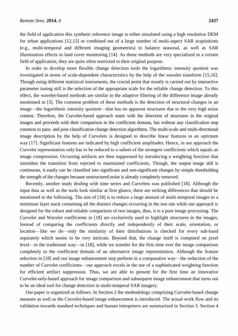
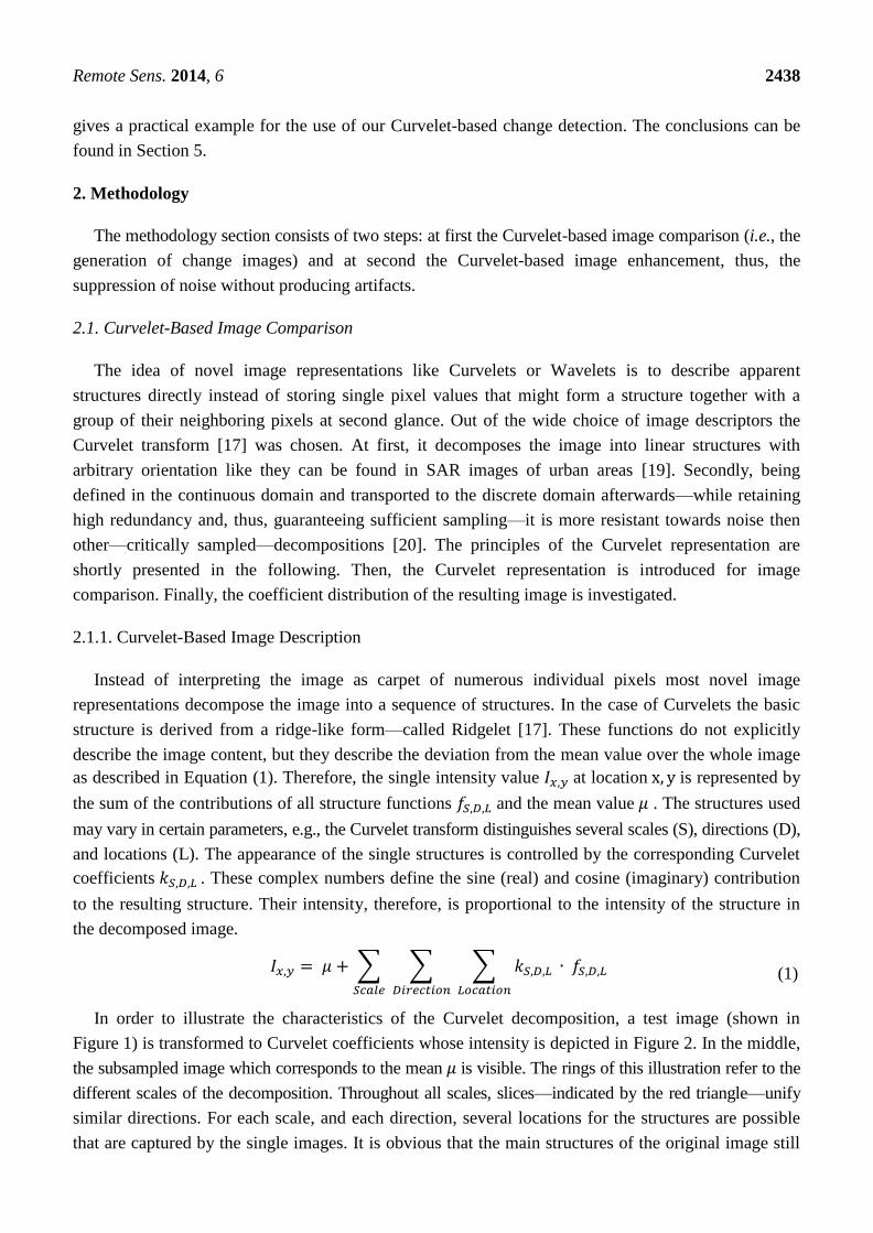
In order to illustrate the characteristics of the Curvelet decomposition, a test image (shown in
Figure 1) is transformed to Curvelet coefficients whose intensity is depicted in Figure 2. In the middle,
the subsampled image which corresponds to the mean is visible. The rings of this illustration refer to the
different scales of the decomposition. Throughout all scales, slices—indicated by the red triangle—unify
similar directions. For each scale, and each direction, several locations for the structures are possible
that are captured by the single images. It is obvious that the main structures of the original image still
Remote Sens. 2014, 6 2439
can be recognized in the coefficient images. However, each single image—indicated by the green
rectangular—highlights special parts of the original image according to scale and direction.
Figure 1. Original—synthetic test image.
Figure 2. Curvelet coefficients intensity of test image—blue ring equates one scale, red
triangle equates one direction, green rectangle equates the locations of one scale and
one direction.
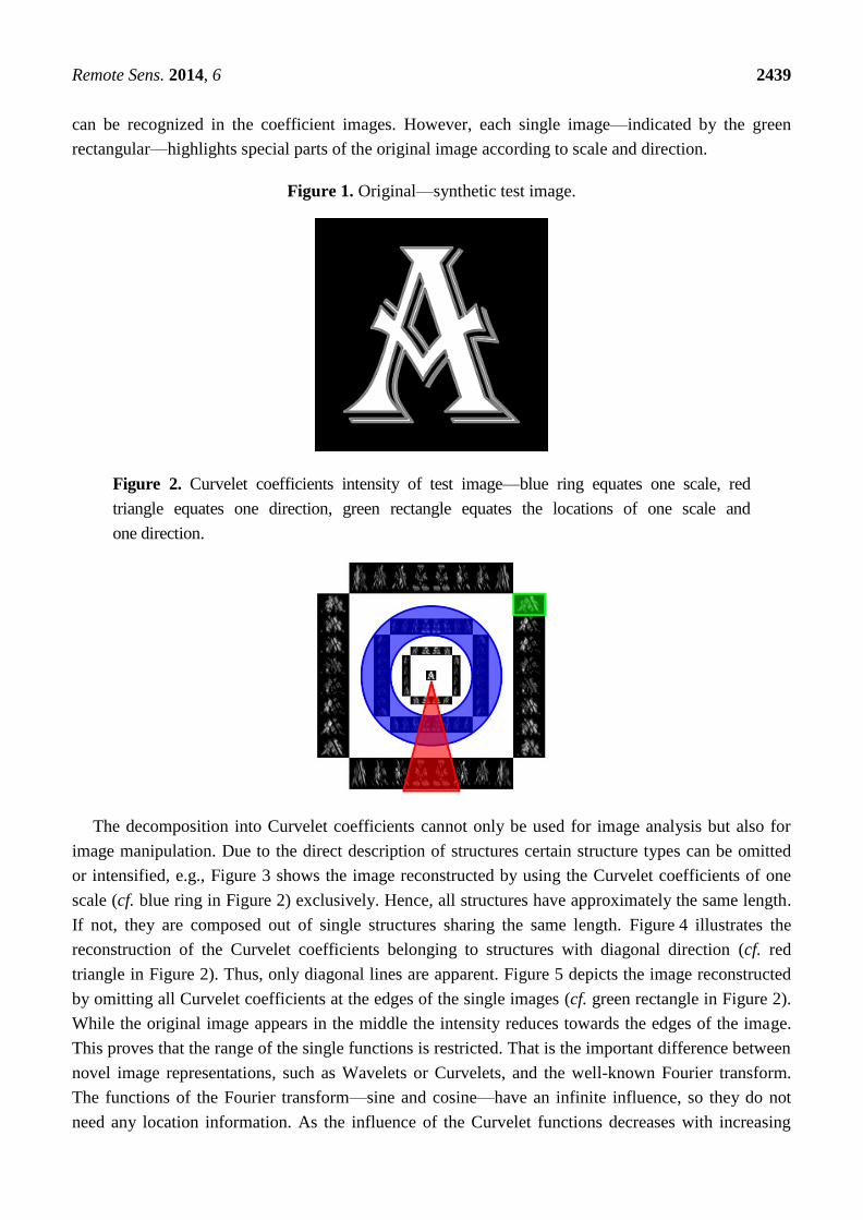
The decomposition into Curvelet coefficients cannot only be used for image analysis but also for
image manipulation. Due to the direct description of structures certain structure types can be omitted
or intensified, e.g., Figure 3 shows the image reconstructed by using the Curvelet coefficients of one
scale (cf. blue ring in Figure 2) exclusively. Hence, all structures have approximately the same length.
If not, they are composed out of single structures sharing the same length. Figure 4 illustrates the
reconstruction of the Curvelet coefficients belonging to structures with diagonal direction (cf. red
triangle in Figure 2). Thus, only diagonal lines are apparent. Figure 5 depicts the image reconstructed
by omitting all Curvelet coefficients at the edges of the single images (cf. green rectangle in Figure 2).
While the original image appears in the middle the intensity reduces towards the edges of the image.
This proves that the range of the single functions is restricted. That is the important difference between
novel image representations, such as Wavelets or Curvelets, and the well-known Fourier transform.
The functions of the Fourier transform—sine and cosine—have an infinite influence, so they do not
need any location information. As the influence of the Curvelet functions decreases with increasing
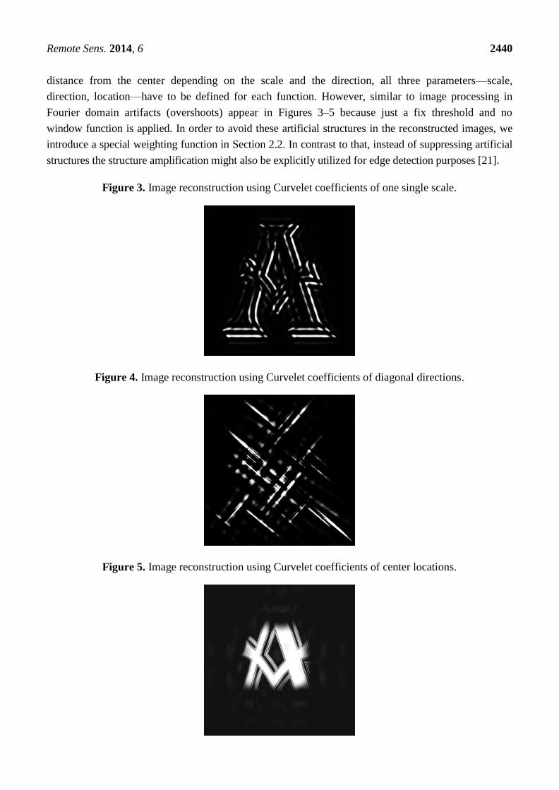
Remote Sens. 2014, 6 2440
distance from the center depending on the scale and the direction, all three parameters—scale,
direction, location—have to be defined for each function. However, similar to image processing in
Fourier domain artifacts (overshoots) appear in Figures 3–5 because just a fix threshold and no
window function is applied. In order to avoid these artificial structures in the reconstructed images, we
introduce a special weighting function in Section 2.2. In contrast to that, instead of suppressing artificial
structures the structure amplification might also be explicitly utilized for edge detection purposes [21].
Figure 3. Image reconstruction using Curvelet coefficients of one single scale.
Figure 4. Image reconstruction using Curvelet coefficients of diagonal directions.
Figure 5. Image reconstruction using Curvelet coefficients of center locations.
Remote Sens. 2014, 6 2441
2.1.2. Curvelet-Based Image Comparison
Due to the multiplicative characteristics of SAR intensity images the intensity quotient in logarithmic
scale is widely used in SAR remote sensing as relative change measure. It can be defined either as
logarithm of the quotient or as difference of the logarithms of the single images, see Equation (2).
(2)
The change image—normally calculated in spatial domain, i.e., pixel by pixel—is highly affected
by noise. As the enhancement of this change measure is a difficult task due to the absence of distinct
structures we try to reformulate the change measure in terms of Curvelet coefficients in Equation (3).
Applying the Curvelet transform ( ) and the inverse Curvelet transform ( ) subsequently to the
single images in the definition taken from Equation (2) does not change Equation (3). The Curvelet
transform outputs the Curvelet coefficients so that the definition in Equation (1) can be inserted into
Equation (3) for both images. Being a linear description, the distribution law applies and the functions
can be differentiated before performing inverse transform. As only the coefficients vary—but, the
function definitions are identical—for two equally sized images, the differentiation even reduces to the
Curvelet coefficients exclusively, see Equation (3).
Thus, the inverse transform of the differential Curvelet coefficients directly results in the change image,
i.e., the logarithm of the intensity quotient. In other words, the structures apparent in the input images can
be transferred to Curvelet coefficients and directly compared by differentiating the corresponding
coefficients which is much more stable than searching for structures in the noisy change image.
(3)
2.1.3. Curvelet Coefficient Statistic
As the Curvelet representation is bijective (i.e., one-to-one and onto), noise is represented as well as
distinct information. But, in contrast to the spatial domain, noise can easily be separated from
structures in the Curvelet coefficient domain. Strong longitudinal structures are known to have higher
coefficients than weaker structures that do not exceed noise level. In order to find the border between
noise and real structure information the distribution of the Curvelet coefficients, i.e., the real and
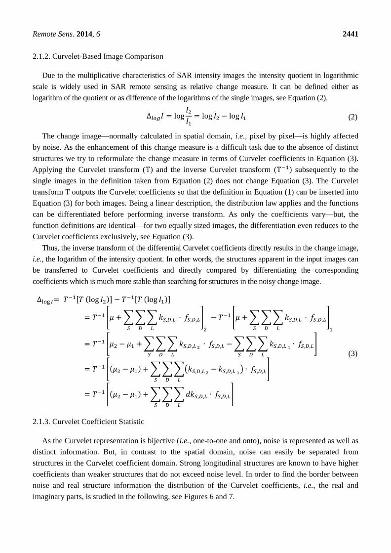
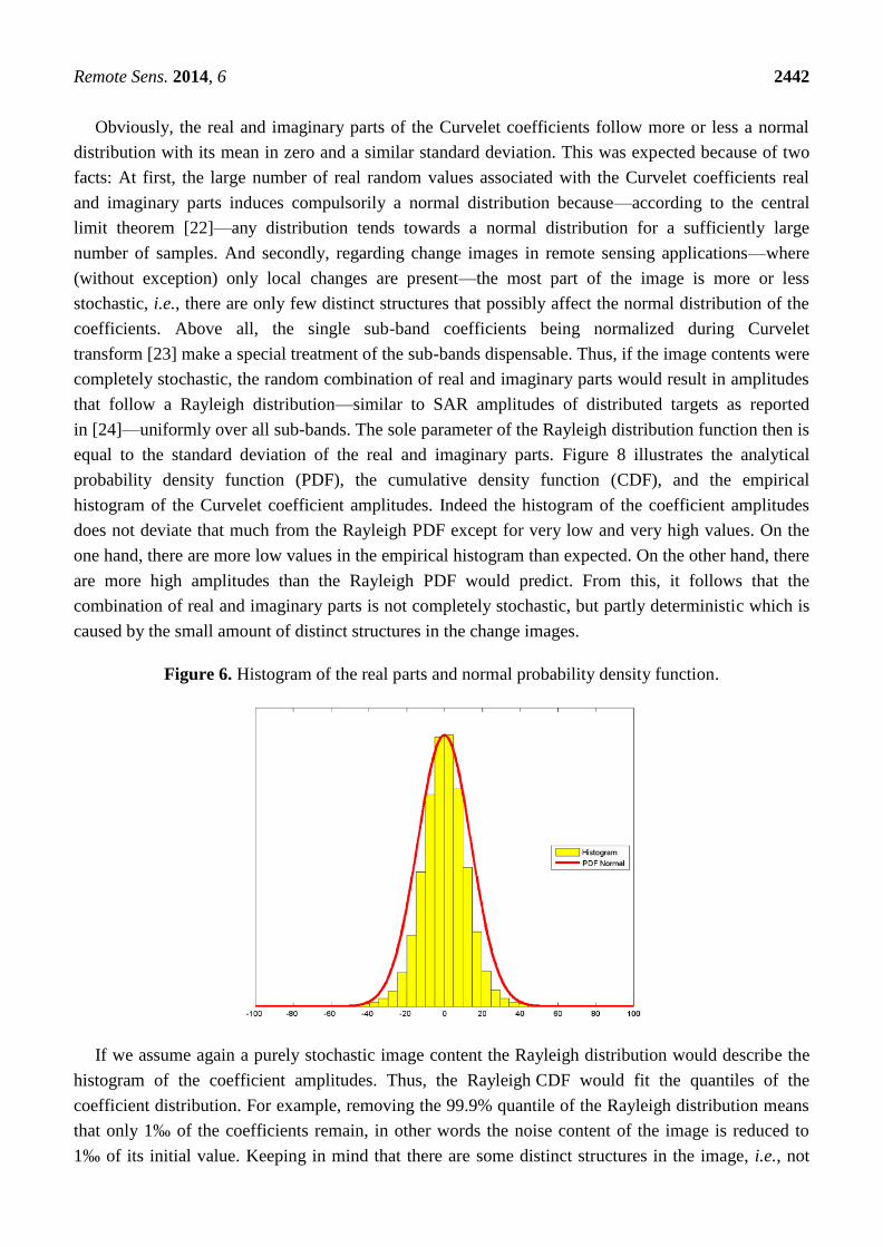
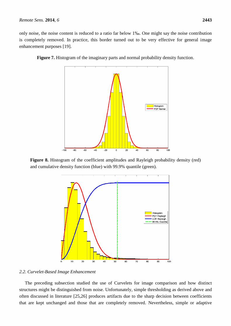
imaginary parts, is studied in the following, see Figures 6 and 7.
Remote Sens. 2014, 6 2442
Obviously, the real and imaginary parts of the Curvelet coefficients follow more or less a normal
distribution with its mean in zero and a similar standard deviation. This was expected because of two
facts: At first, the large number of real random values associated with the Curvelet coefficients real
and imaginary parts induces compulsorily a normal distribution because—according to the central
limit theorem [22]—any distribution tends towards a normal distribution for a sufficiently large
number of samples. And secondly, regarding change images in remote sensing applications—where
(without exception) only local changes are present—the most part of the image is more or less
stochastic, i.e., there are only few distinct structures that possibly affect the normal distribution of the
coefficients. Above all, the single sub-band coefficients being normalized during Curvelet
transform [23] make a special treatment of the sub-bands dispensable. Thus, if the image contents were
completely stochastic, the random combination of real and imaginary parts would result in amplitudes
that follow a Rayleigh distribution—similar to SAR amplitudes of distributed targets as reported
in [24]—uniformly over all sub-bands. The sole parameter of the Rayleigh distribution function then is
equal to the standard deviation of the real and imaginary parts. Figure 8 illustrates the analytical
probability density function (PDF), the cumulative density function (CDF), and the empirical
histogram of the Curvelet coefficient amplitudes. Indeed the histogram of the coefficient amplitudes
does not deviate that much from the Rayleigh PDF except for very low and very high values. On the
one hand, there are more low values in the empirical histogram than expected. On the other hand, there
are more high amplitudes than the Rayleigh PDF would predict. From this, it follows that the
combination of real and imaginary parts is not completely stochastic, but partly deterministic which is
caused by the small amount of distinct structures in the change images.
Figure 6. Histogram of the real parts and normal probability density function.
If we assume again a purely stochastic image content the Rayleigh distribution would describe the
histogram of the coefficient amplitudes. Thus, the Rayleigh CDF would fit the quantiles of the
coefficient distribution. For example, removing the 99.9% quantile of the Rayleigh distribution means
that only 1‰ of the coefficients remain, in other words the noise content of the image is reduced to
1‰ of its initial value. Keeping in mind that there are some distinct structures in the image, i.e., not
Remote Sens. 2014, 6 2443
only noise, the noise content is reduced to a ratio far below 1‰. One might say the noise contribution
is completely removed. In practice, this border turned out to be very effective for general image
enhancement purposes [19].
Figure 7. Histogram of the imaginary parts and normal probability density function.
Figure 8. Histogram of the coefficient amplitudes and Rayleigh probability density (red)
and cumulative density function (blue) with 99.9% quantile (green).
2.2. Curvelet-Based Image Enhancement
The preceding subsection studied the use of Curvelets for image comparison and how distinct
structures might be distinguished from noise. Unfortunately, simple thresholding as derived above and
often discussed in literature [25,26] produces artifacts due to the sharp decision between coefficients
that are kept unchanged and those that are completely removed. Nevertheless, simple or adaptive
Remote Sens. 2014, 6 2444
thresholding still is state of the art in Curvelet-based image denoising [27]. One can refer this behavior
to the image processing in the frequency domain. When certain frequencies are removed from the
entity without applying special window functions, overshoots are produced in general [28]. The effect
is similar to removing certain stationary waves in the Curvelet coefficient domain. If no window
function is defined, the overshoots express in ridge-like artifacts because of the Ridgelet used as basic
element of the Curvelet transform [17]. Therefore, this section will develop a special window function
for Curvelet coefficients—referred to as weighting function in the following—that guarantees a
smooth ascent from suppressed to preserved coefficients and, thus, avoids artifacts in the resulting
change image at the best.
2.2.1. Definition of the Weighting Function
The requested weighting function given in Equation (4) is expected to be continuous as the
Curvelet coefficients can adopt any arbitrary float value. For the sake of convenience, it should be
applied to the differential Curvelet coefficients only before the change image is transformed back to
the spatial domain.
(4)
The difference of the mean values is assumed to be noise-free because of the very high
number of incorporated measurements. Furthermore, as mainly local changes are encountered the
mean differences always range near zero. The coefficients are weighted in relation to their amplitude
solely. Other characteristics, such as scale, direction, location, or the complex phase angle are not
considered because no single scale, direction or location should be preferred to others. As the information
content varies with the number and the strength of changes, the weighting function is adapted to each
change image separately via the corresponding coefficient distribution, see preceding subsection.
2.2.2. Detailed Characteristics of the Weighting Function
Out of the coefficient statistics the two values are calculated that represent the lower border —all
coefficients below that border are completely removed because being addicted to noise—and the upper
border , respectively—all coefficients exceeding this border are seen as distinct structural information
and thus, kept unchanged. In-between the monotonically increasing weighting function applies. At the
borders of the weighted range the function of the weighted coefficients has to meet special
requirements that are summarized in Equation (5).
(5)
At the lower border—symbolized by —the weighted coefficients are set to zero, i.e., their
influence is completely removed. The gradient must be positive. Its absolute value is not defined
exactly. Ideally, the weighting function adapts to a vertical straight line, i.e., with an infinite positive
gradient. At the upper border the value function should reach the bisectrix so that the strength of the
Remote Sens. 2014, 6 2445
coefficients in and above remains unchanged. Additionally, the gradient should reduce to one, and
the curvature should reach zero in order to remain continuous—with respect to the bisectrix—even in
the second derivative. Thus, artifacts caused by widely-used discrete or discontinuous weighting
functions—like simple thresholding—can be avoided. Any function complying with these
prerequisites thus can act as window function for image enhancement based on Curvelet coefficients.
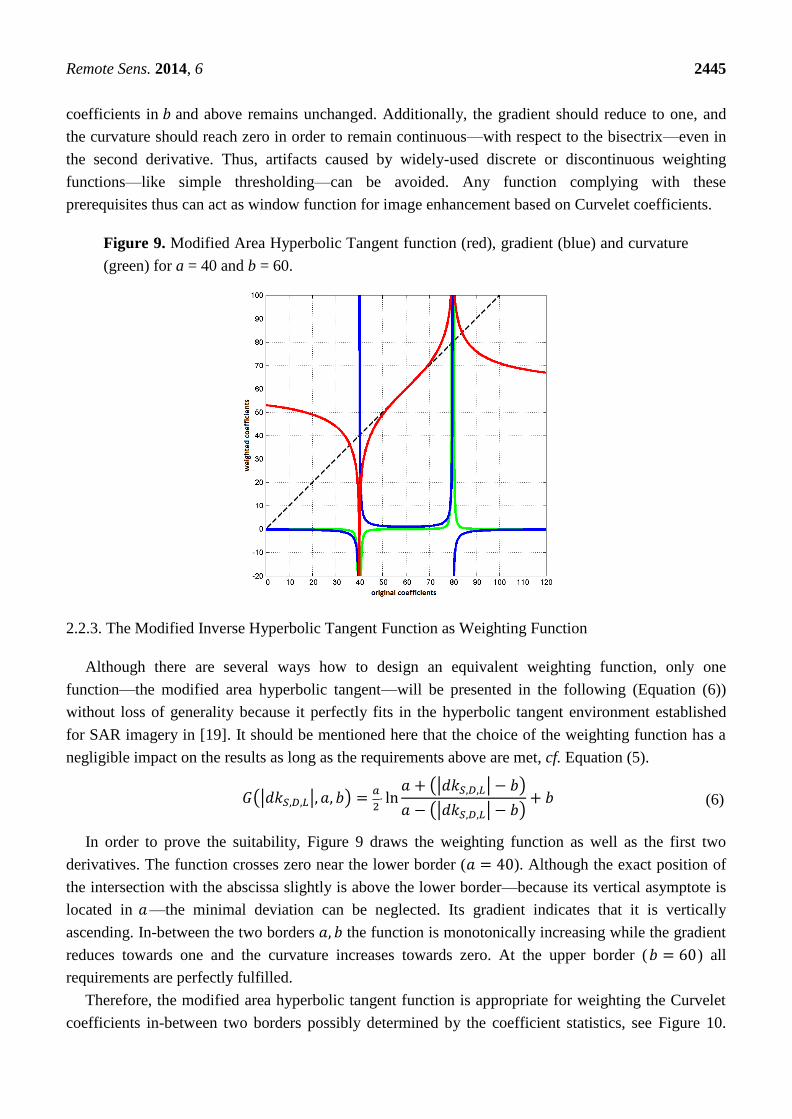
Figure 9. Modified Area Hyperbolic Tangent function (red), gradient (blue) and curvature
(green) for a = 40 and b = 60.
2.2.3. The Modified Inverse Hyperbolic Tangent Function as Weighting Function
Although there are several ways how to design an equivalent weighting function, only one
function—the modified area hyperbolic tangent—will be presented in the following (Equation (6))
without loss of generality because it perfectly fits in the hyperbolic tangent environment established
for SAR imagery in [19]. It should be mentioned here that the choice of the weighting function has a
negligible impact on the results as long as the requirements above are met, cf. Equation (5).
(6)
In order to prove the suitability, Figure 9 draws the weighting function as well as the first two
derivatives. The function crosses zero near the lower border ( ). Although the exact position of
the intersection with the abscissa slightly is above the lower border—because its vertical asymptote is
located in —the minimal deviation can be neglected. Its gradient indicates that it is vertically
ascending. In-between the two borders the function is monotonically increasing while the gradient
reduces towards one and the curvature increases towards zero. At the upper border ( ) all
requirements are perfectly fulfilled.
Therefore, the modified area hyperbolic tangent function is appropriate for weighting the Curvelet
coefficients in-between two borders possibly determined by the coefficient statistics, see Figure 10.
Remote Sens. 2014, 6 2446
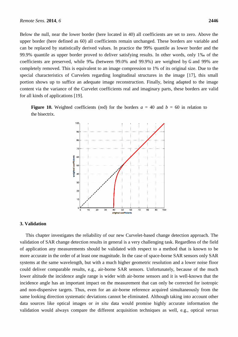
Below the null, near the lower border (here located in 40) all coefficients are set to zero. Above the
upper border (here defined as 60) all coefficients remain unchanged. These borders are variable and
can be replaced by statistically derived values. In practice the 99% quantile as lower border and the
99.9% quantile as upper border proved to deliver satisfying results. In other words, only 1‰ of the
coefficients are preserved, while 9‰ (between 99.0% and 99.9%) are weighted by and 99% are
completely removed. This is equivalent to an image compression to 1% of its original size. Due to the
special characteristics of Curvelets regarding longitudinal structures in the image [17], this small
portion shows up to suffice an adequate image reconstruction. Finally, being adapted to the image
content via the variance of the Curvelet coefficients real and imaginary parts, these borders are valid
for all kinds of applications [19].
Figure 10. Weighted coefficients (red) for the borders a = 40 and b = 60 in relation to
the bisectrix.
3. Validation
This chapter investigates the reliability of our new Curvelet-based change detection approach. The
validation of SAR change detection results in general is a very challenging task. Regardless of the field
of application any measurements should be validated with respect to a method that is known to be
more accurate in the order of at least one magnitude. In the case of space-borne SAR sensors only SAR
systems at the same wavelength, but with a much higher geometric resolution and a lower noise floor
could deliver comparable results, e.g., air-borne SAR sensors. Unfortunately, because of the much
lower altitude the incidence angle range is wider with air-borne sensors and it is well-known that the
incidence angle has an important impact on the measurement that can only be corrected for isotropic
and non-dispersive targets. Thus, even for an air-borne reference acquired simultaneously from the
same looking direction systematic deviations cannot be eliminated. Although taking into account other
data sources like optical images or in situ data would promise highly accurate information the
validation would always compare the different acquisition techniques as well, e.g., optical versus
Remote Sens. 2014, 6 2447
radar. As we aim at validating the Curvelet-based approach against other image interpretation
techniques we decided in favor of a reference produced by experienced human SAR interpreters.
Additionally, two common automated techniques, the simple log-ratio and the log-ratio of
GMAP filtered original images are mentioned as well. For the sake of convenience one 512 ×512 pixel
subset of the HH amplitude of two high resolution spotlight enhanced ellipsoid corrected products
acquired by TerraSAR-X over the industrial harbor of Mannheim (Germany) on 21 September 2008,
and 2 October 2008, respectively (© DLR 2008) is chosen as input though the processing of the whole
scene would also be possible. Both workflows—of the automated and of the manual procedure—are
explained in the following. The results of the comparison conclude this chapter.
3.1. Automated Change Detection
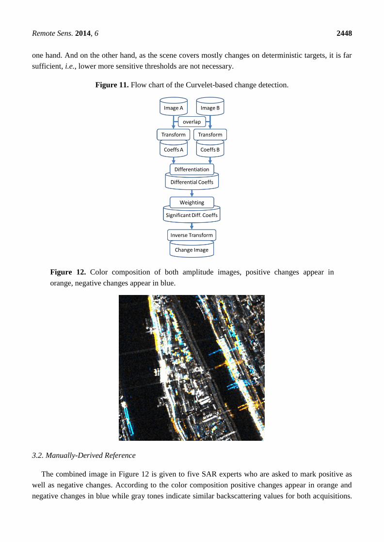
The workflow of the automated approach is given in Figure 11. The procedure starts with the
overlapping parts of two geocoded images (cf. [29]). Thanks to the high quality of the orbit data, no
further co-registration step is necessary for amplitude based change detection as reported in [30]. The
logarithmic intensities of these subsets are transformed into Curvelet coefficients and differentiated in
order to generate the change image. The differential coefficients are subsequently weighted by the
modified area hyperbolic tangent function derived above with the lower border at 1% and the upper
border at 1‰, i.e., in theory 99% of the coefficient are completely removed and only 1‰ of the
coefficients remain unchanged, while all coefficients in-between (from 99.0% to 99.9%) are weighted
continuously. Afterwards the change image is transformed back from the coefficient to the spatial
domain. Both transformations are performed by MATLAB implementations available at [31]
automatically selecting the appropriate number of subbands, rotations, and locations for the optimal
image description with respect to the image dimensions. In the case of the standard techniques the change
image is directly generated as log-ratio of the input images with or without additional speckle suppression.
Figure 12 displays a color composition of the original amplitude images that will be used for
manual classification later on. This test site is deliberately chosen because of the presence of numerous
deterministic scatterers that move in-between the two acquisitions which simplifies the manual change
detection by operators. Human interpreters still providing the most reliable reference we decided to
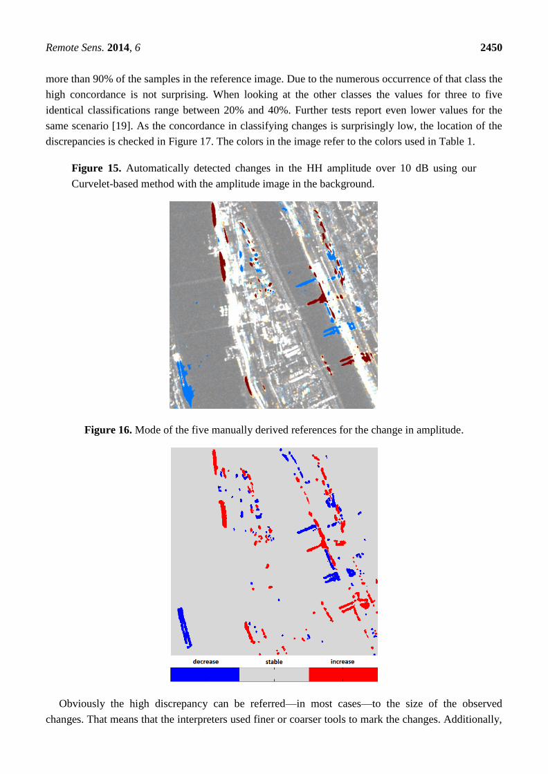
choose this relatively simple scenario. In order to compare our new approach to standard techniques the
pixel-based log-ratios of the radiometrically enhanced TerraSAR-X images [32] incorporating
approximately five looks with and without supplementary speckle suppression using the GMAP
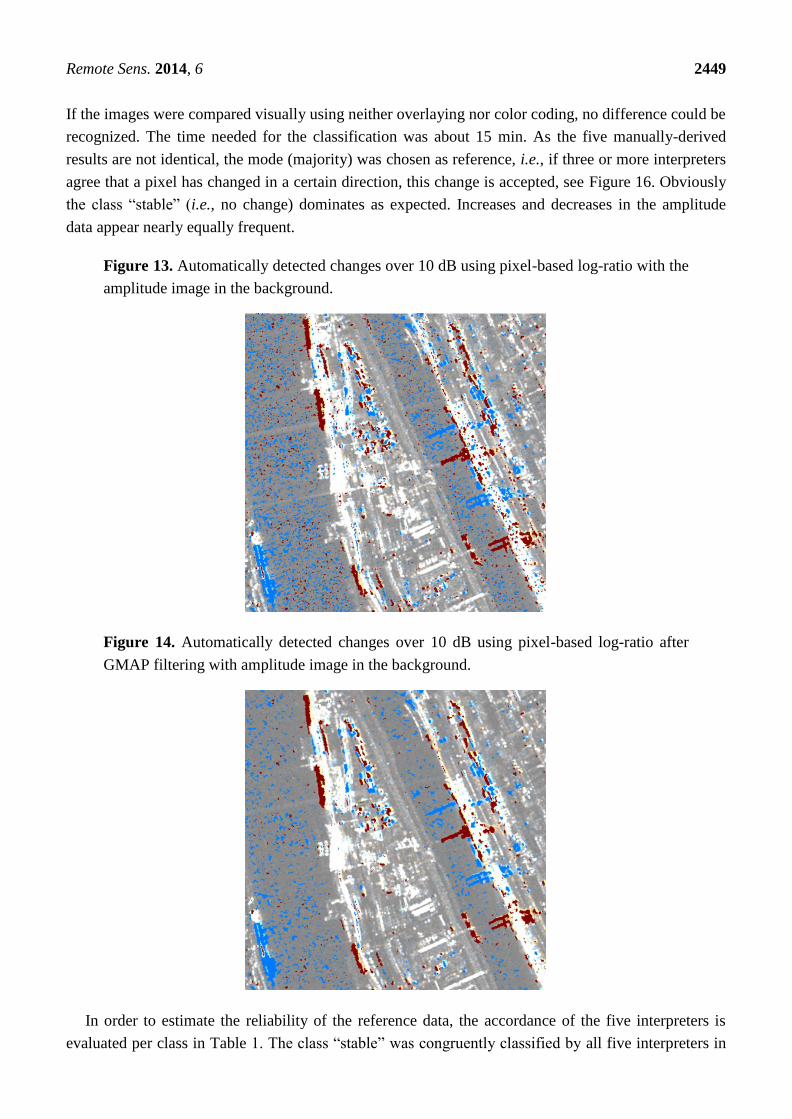
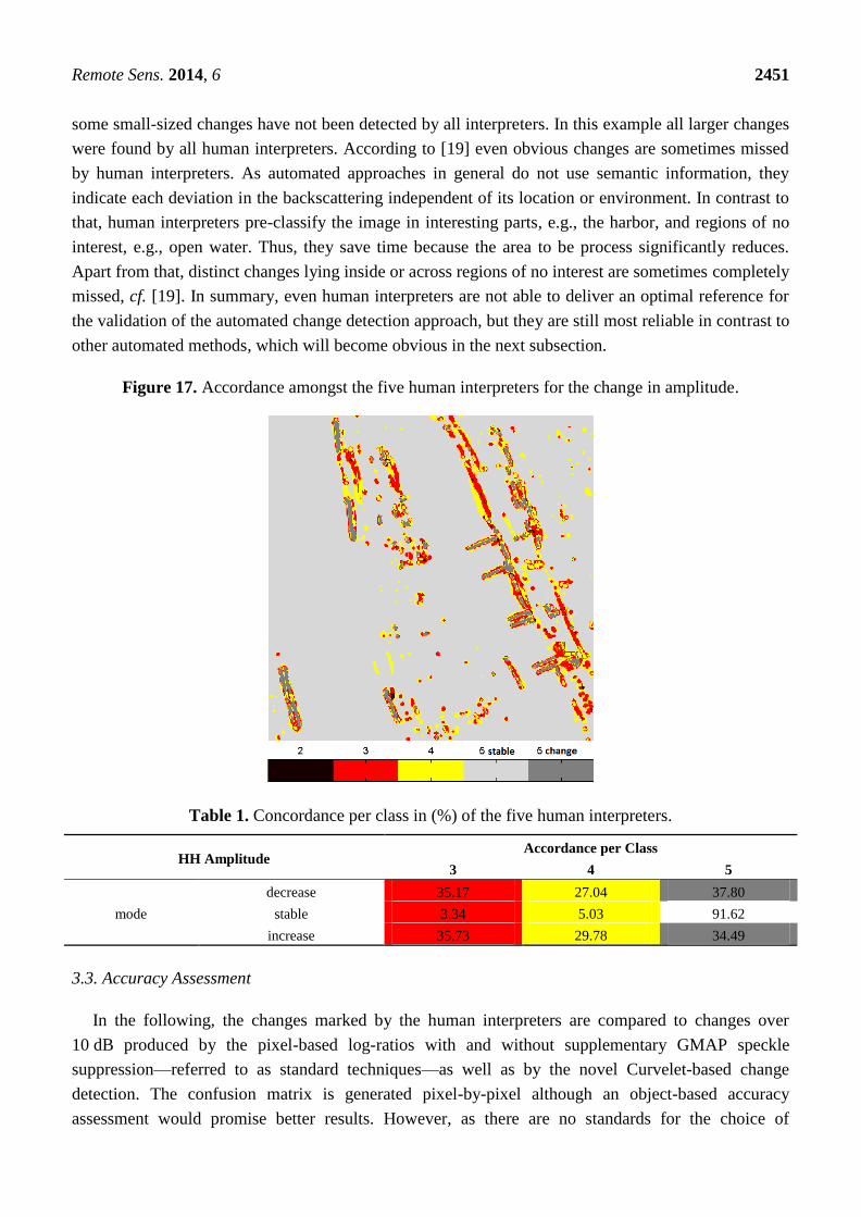
filter [33] are considered as well, see Figures 13 and 14. The results of our automated change detection
approach—performed in 15 seconds by a MATLAB implementation on a SPARC-SOLARIS server—are
shown in Figure 15. Obviously only few distinct structural changes remain after coefficient weighting.
Small-scale changes mainly caused by noise are completely removed while the standard techniques
(Figures 13 and 14) still deliver numerous small change patterns mainly on open water surfaces. The
continuous change image is classified as follows: less than −10 dB equals negative change (in blue),
more than +10 dB equals positive change (in red), otherwise no change detected (transparent). The
high threshold of 10 dB—corresponding to an increase to ten times or a decrease to the tenth of the
original value—is adequate because it is hard for human interpreters to recognize lower changes on the
Remote Sens. 2014, 6 2448
one hand. And on the other hand, as the scene covers mostly changes on deterministic targets, it is far
sufficient, i.e., lower more sensitive thresholds are not necessary.
Figure 11. Flow chart of the Curvelet-based change detection.
Figure 12. Color composition of both amplitude images, positive changes appear in
orange, negative changes appear in blue.
3.2. Manually-Derived Reference
The combined image in Figure 12 is given to five SAR experts who are asked to mark positive as
well as negative changes. According to the color composition positive changes appear in orange and
negative changes in blue while gray tones indicate similar backscattering values for both acquisitions.
Remote Sens. 2014, 6 2449
If the images were compared visually using neither overlaying nor color coding, no difference could be
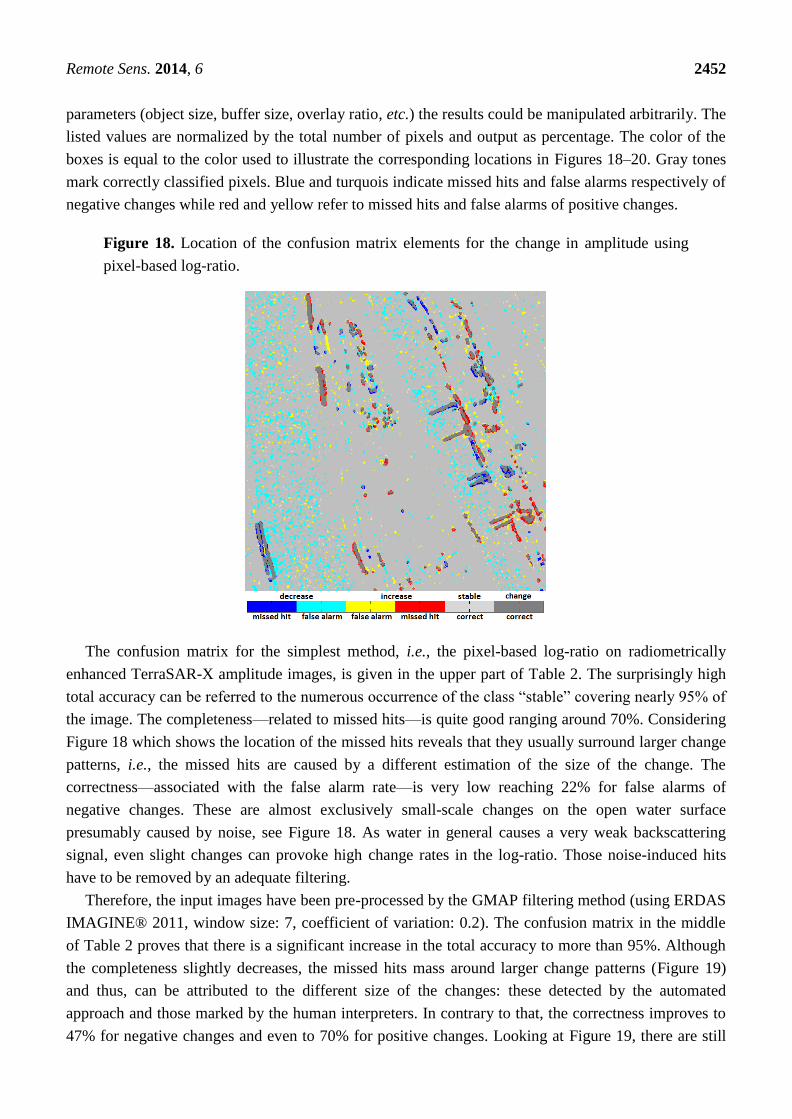
recognized. The time needed for the classification was about 15 min. As the five manually-derived
results are not identical, the mode (majority) was chosen as reference, i.e., if three or more interpreters
agree that a pixel has changed in a certain direction, this change is accepted, see Figure 16. Obviously
the class ―stable‖ (i.e., no change) dominates as expected. Increases and decreases in the amplitude
data appear nearly equally frequent.
Figure 13. Automatically detected changes over 10 dB using pixel-based log-ratio with the
amplitude image in the background.
Figure 14. Automatically detected changes over 10 dB using pixel-based log-ratio after
GMAP filtering with amplitude image in the background.
In order to estimate the reliability of the reference data, the accordance of the five interpreters is
evaluated per class in Table 1. The class ―stable‖ was congruently classified by all five interpreters in
Remote Sens. 2014, 6 2450
more than 90% of the samples in the reference image. Due to the numerous occurrence of that class the
high concordance is not surprising. When looking at the other classes the values for three to five
identical classifications range between 20% and 40%. Further tests report even lower values for the
same scenario [19]. As the concordance in classifying changes is surprisingly low, the location of the
discrepancies is checked in Figure 17. The colors in the image refer to the colors used in Table 1.
Figure 15. Automatically detected changes in the HH amplitude over 10 dB using our
Curvelet-based method with the amplitude image in the background.
Figure 16. Mode of the five manually derived references for the change in amplitude.
Obviously the high discrepancy can be referred—in most cases—to the size of the observed
changes. That means that the interpreters used finer or coarser tools to mark the changes. Additionally,
Remote Sens. 2014, 6 2451
some small-sized changes have not been detected by all interpreters. In this example all larger changes
were found by all human interpreters. According to [19] even obvious changes are sometimes missed
by human interpreters. As automated approaches in general do not use semantic information, they
indicate each deviation in the backscattering independent of its location or environment. In contrast to
that, human interpreters pre-classify the image in interesting parts, e.g., the harbor, and regions of no
interest, e.g., open water. Thus, they save time because the area to be process significantly reduces.
Apart from that, distinct changes lying inside or across regions of no interest are sometimes completely
missed, cf. [19]. In summary, even human interpreters are not able to deliver an optimal reference for
the validation of the automated change detection approach, but they are still most reliable in contrast to
other automated methods, which will become obvious in the next subsection.
Figure 17. Accordance amongst the five human interpreters for the change in amplitude.
Table 1. Concordance per class in (%) of the five human interpreters.
HH Amplitude Accordance per Class
3 4 5
mode
decrease 35.17 27.04 37.80
stable 3.34 5.03 91.62
increase 35.73 29.78 34.49
3.3. Accuracy Assessment
In the following, the changes marked by the human interpreters are compared to changes over
10 dB produced by the pixel-based log-ratios with and without supplementary GMAP speckle
suppression—referred to as standard techniques—as well as by the novel Curvelet-based change
detection. The confusion matrix is generated pixel-by-pixel although an object-based accuracy
assessment would promise better results. However, as there are no standards for the choice of
Remote Sens. 2014, 6 2452
parameters (object size, buffer size, overlay ratio, etc.) the results could be manipulated arbitrarily. The
listed values are normalized by the total number of pixels and output as percentage. The color of the
boxes is equal to the color used to illustrate the corresponding locations in Figures 18–20. Gray tones
mark correctly classified pixels. Blue and turquois indicate missed hits and false alarms respectively of
negative changes while red and yellow refer to missed hits and false alarms of positive changes.
Figure 18. Location of the confusion matrix elements for the change in amplitude using
pixel-based log-ratio.
The confusion matrix for the simplest method, i.e., the pixel-based log-ratio on radiometrically
enhanced TerraSAR-X amplitude images, is given in the upper part of Table 2. The surprisingly high
total accuracy can be referred to the numerous occurrence of the class ―stable‖ covering nearly 95% of
the image. The completeness—related to missed hits—is quite good ranging around 70%. Considering
Figure 18 which shows the location of the missed hits reveals that they usually surround larger change
patterns, i.e., the missed hits are caused by a different estimation of the size of the change. The
correctness—associated with the false alarm rate—is very low reaching 22% for false alarms of
negative changes. These are almost exclusively small-scale changes on the open water surface
presumably caused by noise, see Figure 18. As water in general causes a very weak backscattering
signal, even slight changes can provoke high change rates in the log-ratio. Those noise-induced hits
have to be removed by an adequate filtering.
Therefore, the input images have been pre-processed by the GMAP filtering method (using ERDAS
IMAGINE® 2011, window size: 7, coefficient of variation: 0.2). The confusion matrix in the middle
of Table 2 proves that there is a significant increase in the total accuracy to more than 95%. Although
the completeness slightly decreases, the missed hits mass around larger change patterns (Figure 19)
and thus, can be attributed to the different size of the changes: these detected by the automated
approach and those marked by the human interpreters. In contrary to that, the correctness improves to
47% for negative changes and even to 70% for positive changes. Looking at Figure 19, there are still
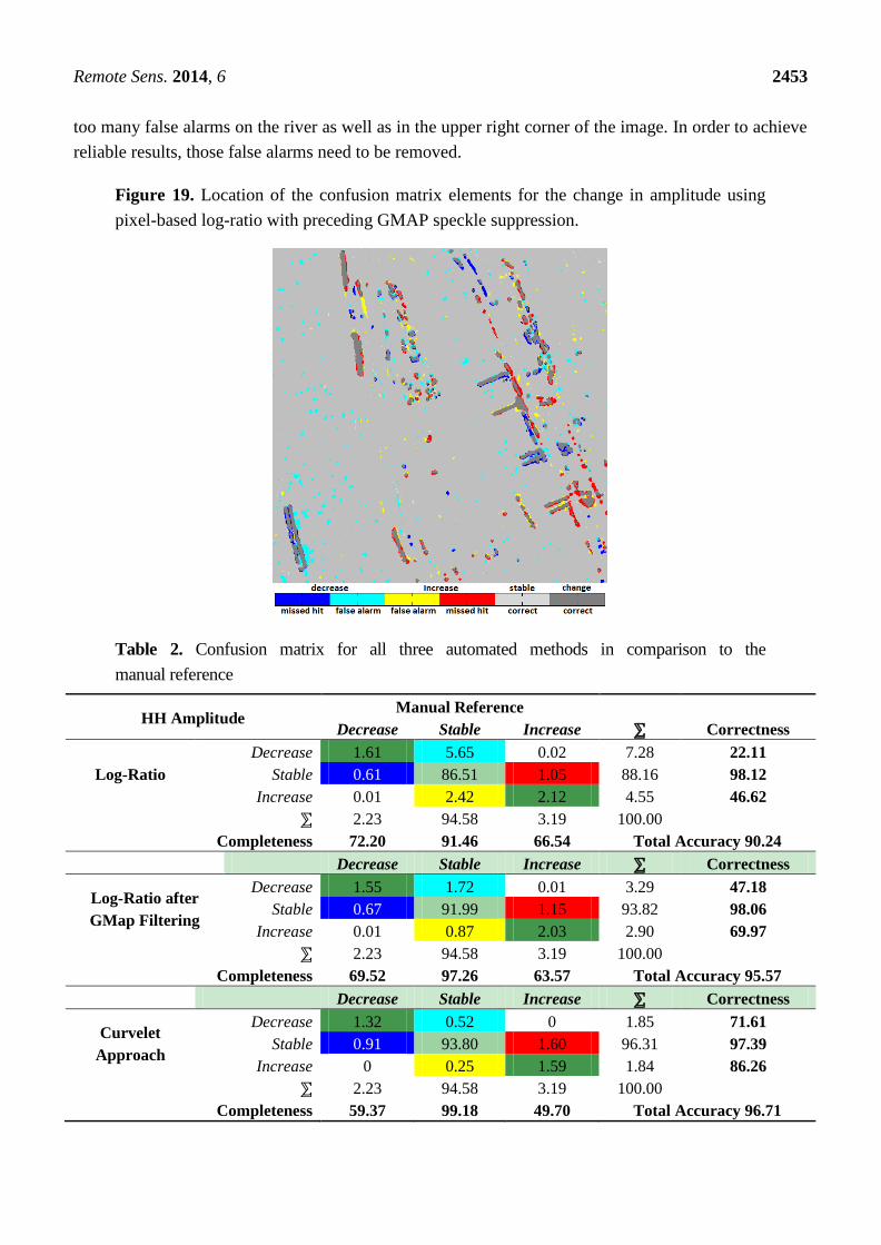
Remote Sens. 2014, 6 2453
too many false alarms on the river as well as in the upper right corner of the image. In order to achieve
reliable results, those false alarms need to be removed.
Figure 19. Location of the confusion matrix elements for the change in amplitude using
pixel-based log-ratio with preceding GMAP speckle suppression.
Table 2. Confusion matrix for all three automated methods in comparison to the
manual reference
HH Amplitude Manual Reference
Decrease Stable Increase ⅀ Correctness
Log-Ratio
Decrease 1.61 5.65 0.02 7.28 22.11
Stable 0.61 86.51 1.05 88.16 98.12
Increase 0.01 2.42 2.12 4.55 46.62
⅀ 2.23 94.58 3.19 100.00
Completeness 72.20 91.46 66.54 Total Accuracy 90.24
Decrease Stable Increase ⅀ Correctness
Log-Ratio after
GMap Filtering
Decrease 1.55 1.72 0.01 3.29 47.18
Stable 0.67 91.99 1.15 93.82 98.06
Increase 0.01 0.87 2.03 2.90 69.97
⅀ 2.23 94.58 3.19 100.00
Completeness 69.52 97.26 63.57 Total Accuracy 95.57
Decrease Stable Increase ⅀ Correctness
Curvelet
Approach
Decrease 1.32 0.52 0 1.85 71.61
Stable 0.91 93.80 1.60 96.31 97.39
Increase 0 0.25 1.59 1.84 86.26
⅀ 2.23 94.58 3.19 100.00
Completeness 59.37 99.18 49.70 Total Accuracy 96.71
Remote Sens. 2014, 6 2454
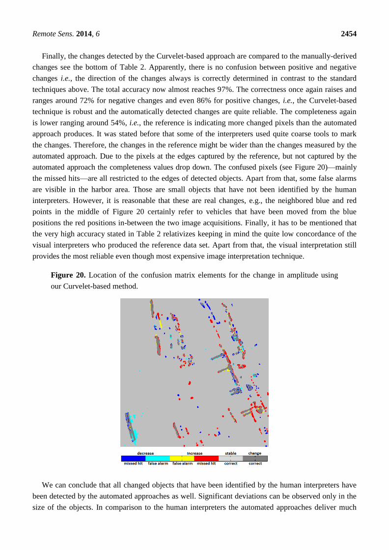
Finally, the changes detected by the Curvelet-based approach are compared to the manually-derived
changes see the bottom of Table 2. Apparently, there is no confusion between positive and negative
changes i.e., the direction of the changes always is correctly determined in contrast to the standard
techniques above. The total accuracy now almost reaches 97%. The correctness once again raises and
ranges around 72% for negative changes and even 86% for positive changes, i.e., the Curvelet-based
technique is robust and the automatically detected changes are quite reliable. The completeness again
is lower ranging around 54%, i.e., the reference is indicating more changed pixels than the automated
approach produces. It was stated before that some of the interpreters used quite coarse tools to mark
the changes. Therefore, the changes in the reference might be wider than the changes measured by the
automated approach. Due to the pixels at the edges captured by the reference, but not captured by the
automated approach the completeness values drop down. The confused pixels (see Figure 20)—mainly
the missed hits—are all restricted to the edges of detected objects. Apart from that, some false alarms
are visible in the harbor area. Those are small objects that have not been identified by the human
interpreters. However, it is reasonable that these are real changes, e.g., the neighbored blue and red
points in the middle of Figure 20 certainly refer to vehicles that have been moved from the blue
positions the red positions in-between the two image acquisitions. Finally, it has to be mentioned that
the very high accuracy stated in Table 2 relativizes keeping in mind the quite low concordance of the
visual interpreters who produced the reference data set. Apart from that, the visual interpretation still
provides the most reliable even though most expensive image interpretation technique.
Figure 20. Location of the confusion matrix elements for the change in amplitude using
our Curvelet-based method.
We can conclude that all changed objects that have been identified by the human interpreters have
been detected by the automated approaches as well. Significant deviations can be observed only in the
size of the objects. In comparison to the human interpreters the automated approaches deliver much
Remote Sens. 2014, 6 2455
faster and in general more complete results. But, the reliability of the indicated changes is highly
variable. None of the standard techniques tested here could compete with our Curvelet-based approach
in reducing the false alarm rate and, thus, guaranteeing reliable results. In contrast to the visual
interpretation, the automated methods are repeatable: Even if the same image was given to same human
interpreter several times, each product will be different from the others [19]. However, human interpreters
are able to pre-classify the image and then distinguish between changes of interest (e.g., changes on
industrial facilities) and changes of no interest (e.g., changes on water surfaces caused by varying wind
conditions). For automated approaches, this ―masking‖ of areas of interest has to be done in a further
step using additional geo-information on the land cover in the observed scene.
4. Application
Now that the suitability of the novel Curvelet-based change detection approach is proven, the
method can be applied to longer time series. In the following, the multi-temporal images are shortly
presented, as well as the changes detected by the Curvelet-based approach. The last section of this
chapter explains how these results can easily be utilized for construction site monitoring.
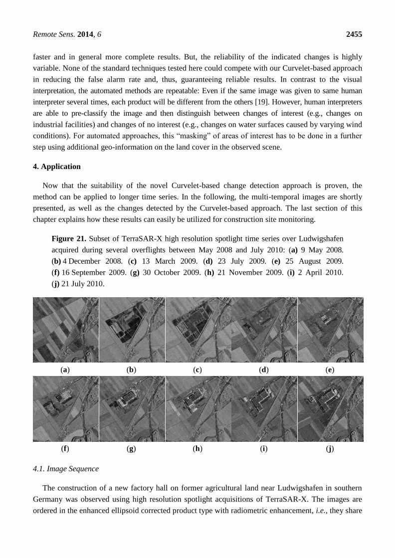
Figure 21. Subset of TerraSAR-X high resolution spotlight time series over Ludwigshafen
acquired during several overflights between May 2008 and July 2010: (a) 9 May 2008.
(b) 4 December 2008. (c) 13 March 2009. (d) 23 July 2009. (e) 25 August 2009.
(f) 16 September 2009. (g) 30 October 2009. (h) 21 November 2009. (i) 2 April 2010.
(j) 21 July 2010.
(a) (b) (c) (d) (e)
(f) (g) (h) (i) (j)
4.1. Image Sequence
The construction of a new factory hall on former agricultural land near Ludwigshafen in southern
Germany was observed using high resolution spotlight acquisitions of TerraSAR-X. The images are
ordered in the enhanced ellipsoid corrected product type with radiometric enhancement, i.e., they share
Remote Sens. 2014, 6 2456
a nominal look factor of about 7.6 and a corresponding pixel spacing of 1.25 m. Due to the high
accuracy of the science orbit data—less than one decimeter—no further co-registration is necessary.
As the first images are already acquired, long before the start of the construction, and also during
winter time—where no construction activities take place—only ten images out of the dense time series
are chosen that represent the main steps in the construction progress, see Figure 21. The first image
still displays the former rural landscape on 9 May 2008, before the construction works begin. In the
second image from 4 December 2008, earthwork already started. Arising brighter points indicate new
parts of the future building in the following images taken on 13 March 2009, 23 July 2009, 25 August
2009, 16 September 2009, 30 October 2009, 21 November 2009, and 2 April 2010. The last image
depicts the final building complex on 21 July 2010. Fortunately, the constructor documented the
construction progress in his internet presence [34] in a very detailed manner so that we can easily
check the reliability of our observations.
4.2. Detected Changes
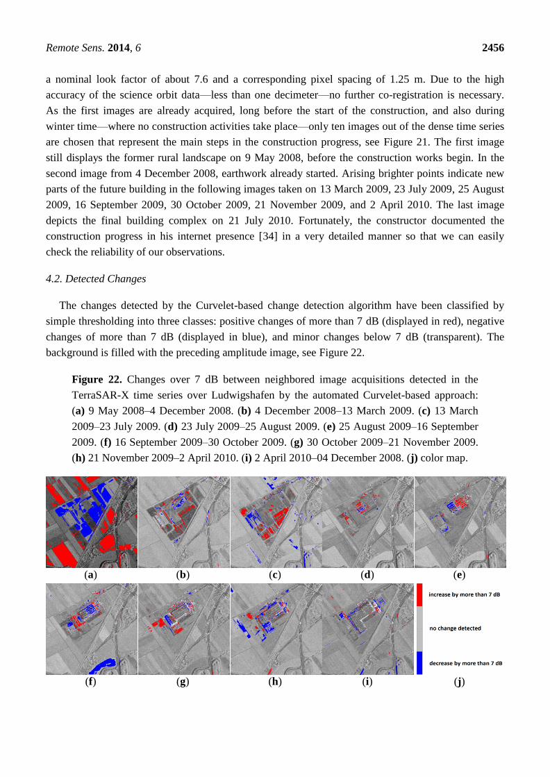
The changes detected by the Curvelet-based change detection algorithm have been classified by
simple thresholding into three classes: positive changes of more than 7 dB (displayed in red), negative
changes of more than 7 dB (displayed in blue), and minor changes below 7 dB (transparent). The
background is filled with the preceding amplitude image, see Figure 22.
Figure 22. Changes over 7 dB between neighbored image acquisitions detected in the
TerraSAR-X time series over Ludwigshafen by the automated Curvelet-based approach:
(a) 9 May 2008–4 December 2008. (b) 4 December 2008–13 March 2009. (c) 13 March
2009–23 July 2009. (d) 23 July 2009–25 August 2009. (e) 25 August 2009–16 September
2009. (f) 16 September 2009–30 October 2009. (g) 30 October 2009–21 November 2009.
(h) 21 November 2009–2 April 2010. (i) 2 April 2010–04 December 2008. (j) color map.
(a) (b) (c) (d) (e)
(f) (g) (h) (i) (j)
Remote Sens. 2014, 6 2457
The first change detection image Figure 22a mainly consists of large-scale changes on the future
construction site and on the surrounding agricultural fields as well. However, in contrast to the fields a
negative change is observed due to beginning earth moving activities. The following two time steps (b)
and (c) indicate the progress in earthworks. Additionally, several small-scale changes along the road
are visible which can be referred to traffic. Due to the shift of moving objects in SAR these changes
often lay beside the road [35]. Change image (d) shows parallel dotted lines in the middle of the image
in red, i.e., these are new objects. The same objects appear in blue, i.e., they disappear, in the next step
(e), but new dotted lines in red are added. The same behavior can be observed for the following two
steps (f) and (g): new objects appear and disappear again in the next time step.
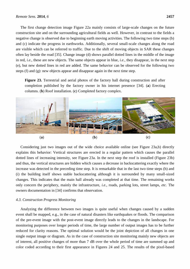
Figure 23. Terrestrial and aerial photos of the factory hall during construction and after
completion published by the factory owner in his internet presence [34]. (a) Erecting
columns. (b) Roof installation. (c) Completed factory complex.
(a) (b) (c)
Considering just two images out of the wide choice available online (see Figure 23a,b) directly
explains this behavior: Vertical structures are erected in a regular pattern which causes the parallel
dotted lines of increasing intensity, see Figure 23a. In the next step the roof is installed (Figure 23b)
and thus, the vertical structures are hidden which causes a decrease in backscattering exactly where the
increase was detected in the preceding time step. It is remarkable that in the last two time steps (h) and
(i) the building itself shows stable backscattering although it is surrounded by many small-sized
changes. This indicates that the main hall already was completed at that time. The remaining works
only concern the periphery, mainly the infrastructure, i.e., roads, parking lots, street lamps, etc. The
owners documentation in [34] confirms that observation.
4.3. Construction Progress Monitoring
Analyzing the difference between two images is quite useful when changes caused by a sudden
event shall be mapped, e.g., in the case of natural disasters like earthquakes or floods. The comparison
of the pre-event image with the post-event image directly leads to the changes in the landscape. For
monitoring purposes over longer periods of time, the large number of output images has to be further
reduced for clarity reasons. The optimal solution would be the joint depiction of all changes in one
single output image or diagram. As in the case of construction site monitoring mainly new objects are
of interest, all positive changes of more than 7 dB over the whole period of time are summed up and
color coded according to their first appearance in Figures 24 and 25. The results of the pixel-based
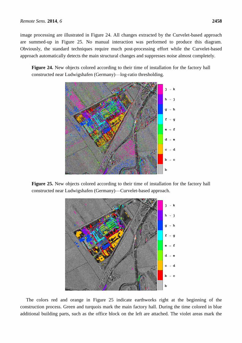
Remote Sens. 2014, 6 2458
image processing are illustrated in Figure 24. All changes extracted by the Curvelet-based approach
are summed-up in Figure 25. No manual interaction was performed to produce this diagram.
Obviously, the standard techniques require much post-processing effort while the Curvelet-based
approach automatically detects the main structural changes and suppresses noise almost completely.
Figure 24. New objects colored according to their time of installation for the factory hall
constructed near Ludwigshafen (Germany)—log-ratio thresholding.
Figure 25. New objects colored according to their time of installation for the factory hall
constructed near Ludwigshafen (Germany)—Curvelet-based approach.
The colors red and orange in Figure 25 indicate earthworks right at the beginning of the
construction process. Green and turquois mark the main factory hall. During the time colored in blue
additional building parts, such as the office block on the left are attached. The violet areas mark the
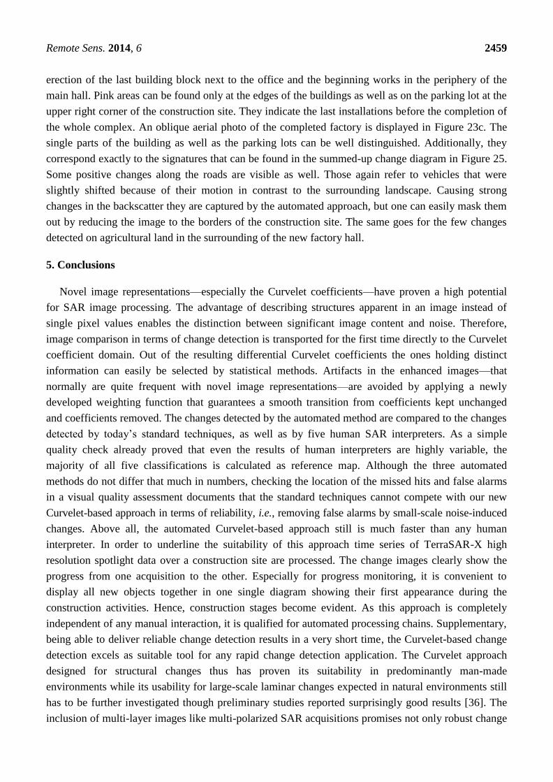
Remote Sens. 2014, 6 2459
erection of the last building block next to the office and the beginning works in the periphery of the
main hall. Pink areas can be found only at the edges of the buildings as well as on the parking lot at the
upper right corner of the construction site. They indicate the last installations before the completion of
the whole complex. An oblique aerial photo of the completed factory is displayed in Figure 23c. The
single parts of the building as well as the parking lots can be well distinguished. Additionally, they
correspond exactly to the signatures that can be found in the summed-up change diagram in Figure 25.
Some positive changes along the roads are visible as well. Those again refer to vehicles that were
slightly shifted because of their motion in contrast to the surrounding landscape. Causing strong
changes in the backscatter they are captured by the automated approach, but one can easily mask them
out by reducing the image to the borders of the construction site. The same goes for the few changes
detected on agricultural land in the surrounding of the new factory hall.
5. Conclusions
Novel image representations—especially the Curvelet coefficients—have proven a high potential
for SAR image processing. The advantage of describing structures apparent in an image instead of
single pixel values enables the distinction between significant image content and noise. Therefore,
image comparison in terms of change detection is transported for the first time directly to the Curvelet
coefficient domain. Out of the resulting differential Curvelet coefficients the ones holding distinct
information can easily be selected by statistical methods. Artifacts in the enhanced images—that
normally are quite frequent with novel image representations—are avoided by applying a newly
developed weighting function that guarantees a smooth transition from coefficients kept unchanged
and coefficients removed. The changes detected by the automated method are compared to the changes
detected by today’s standard techniques, as well as by five human SAR interpreters. As a simple
quality check already proved that even the results of human interpreters are highly variable, the
majority of all five classifications is calculated as reference map. Although the three automated
methods do not differ that much in numbers, checking the location of the missed hits and false alarms
in a visual quality assessment documents that the standard techniques cannot compete with our new
Curvelet-based approach in terms of reliability, i.e., removing false alarms by small-scale noise-induced
changes. Above all, the automated Curvelet-based approach still is much faster than any human
interpreter. In order to underline the suitability of this approach time series of TerraSAR-X high
resolution spotlight data over a construction site are processed. The change images clearly show the
progress from one acquisition to the other. Especially for progress monitoring, it is convenient to
display all new objects together in one single diagram showing their first appearance during the
construction activities. Hence, construction stages become evident. As this approach is completely
independent of any manual interaction, it is qualified for automated processing chains. Supplementary,
being able to deliver reliable change detection results in a very short time, the Curvelet-based change
detection excels as suitable tool for any rapid change detection application. The Curvelet approach
designed for structural changes thus has proven its suitability in predominantly man-made
environments while its usability for large-scale laminar changes expected in natural environments still
has to be further investigated though preliminary studies reported surprisingly good results [36]. The
inclusion of multi-layer images like multi-polarized SAR acquisitions promises not only robust change
Remote Sens. 2014, 6 2460
detection results, but even a detailed change characterization which has already shown a high potential in
wetland monitoring, cf., previous studies in [37]. At last, this innovative Curvelet-only-based image
comparison technique—though developed and presented in the context of SAR remote sensing—turned
out to be suitable for numerous other robust change detection purposes based on any kind of noisy
image data during preliminary studies.
Acknowledgments
The TerraSAR-X acquisitions used as input were provided under the Proposal LAN0481 titled
―Polarimetry in urban areas‖. The MATLAB® implementation of the Curvelet transform was
downloaded from ―Curvelet.org‖ (version 2.1.2 April 2008). Thanks to the Curvelet.org team
(Emmanuel Candes, Laurent Demanet, David Donoho, Lexing Ying) for providing the software.
Finally, the authors like to thank the five SAR interpreters from the German Remote Sensing Data
Center for generating reference data.
Author contribution
Andreas Schmitt is the principal author of this paper. The technique presented here is one facet of
his research activities at the German Aerospace Center (DLR) over the last few years. Birgit Wessel
and Achim Roth supervised his work.
Conflicts of Interest
The authors declare no conflict of interest.
References and Notes
1. Carincotte, C.; Derrode, S.; Bourennane, S. Unsupervised change detection on SAR images using
fuzzy hidden Markov chains. IEEE Trans. Geosci. Remote Sens. 2006, 44, 432–441.
2. Gamba, P.; Dell’Acqua, F.; Lisini, G. Change detection of multitemporal SAR data in urban areas
combining feature-based and pixel-based techniques. IEEE Trans. Geosci. Remote Sens. 2006, 44,
2820–2827.
3. Dekker, R.J. SAR Change Detection Techniques and Applications. In Proceedings of 25th
EARSeL Symposium on Global Developments in Environmental Earth Observation from Space,
Porto, Portugal, 6–11 June 2005.
4. Liu, W.; Yamazaki, F. Urban Monitoring and Change Detection of Central Tokyo Using
TerraSAR-X Images. In Proceedings of 2011 IEEE International Geoscience and Remote Sensing
Symposium, Vancouver, BC, Canada, 24–29 July 2011.
5. Liao, M.; Jiang, L.; Lin, H.; Huang, B.; Gong, J. Urban change detection based on coherence and
intensity characteristics of SAR imagery. Photogramm. Eng. Remote Sens. 2008, 74, 999–1006.
6. Derrode, S.; Mercier, G.; Pieczynski, W. Unsupervised Change Detection in SAR Images Using a
Multicomponent HMC Model. In Proceedings of the Second International Workshop on
Multi-temp’03, Ispra, Italy, 16–18 July 2003.
Remote Sens. 2014, 6 2461
7. Bouyahia, Z.; Benyoussef, L.; Derrode, S. Change detection in synthetic aperture radar images
with a sliding hidden Markov chain model. J. Appl. Remote Sens. 2008, doi:10.1117/1.2957968.
8. Conradsen, K.; Nielsen, A.A.; Schou, J.; Skriver, H. A test statistic in the complex Wishart
distribution and its application to change detection in polarimetric SAR data. IEEE Trans. Geosci.
Remote Sens. 2003, 41, 4–19.
9. Erten, E. Information Theory of Multi-Temporal SAR Systems with Application to Motion
Detection and Change Detection. Ph.D. Thesis, Technical University of Berlin, Berlin, Germany,
November 2010.
10. Ban, Y.; Yousif, O.A. Multitemporal spaceborne SAR data for urban change detection in China.
IEEE Sel. Top. Appl. Earth Obs. Remote Sens. 2012, 5, 1087–1094.
11. Shan, Z.; Wang, C.; Zhang, H.; Wu, F. Change Detection in Urban Areas with High Resolution
SAR Images Using Second Kind Statistics based G0 Distribution. In Proceedings of 2010 IEEE
International Geoscience and Remote Sensing Symposium, Honolulu, HI, USA, 25–30 July 2010.
12. Auer, S.; Balz, T.; Becker, S.; Bamler, R. 3D SAR simulation of urban areas based on detailed
building models. Photogramm. Eng. Remote Sens. 2010, 76, 1373–1384.
13. Balz, T. SAR Simulation based Change Detection with High-Resolution SAR Images in Urban
Environments. Int. Arch. Photogramm. Remote Sens. Spat. Inf. Sci. 2004, 35, 472–477.
14. Romero, R.; Sanz-Marcos, J.; Carrasco, D.; Moreno, V.; Valero, J.L.; Lafitte, M. SAR
Superresolution Change Detection for Security Applications. In Proceedings of Envisat Symposium
2007, Montreux, Switzerland, 23–27 April, 2007.
15. Cui, S.; Datcu, M. Statistical wavelet subband modeling for multi-temporal SAR change detection.
IEEE J. Sel. Top. Appl. Earth Obs. Remote Sens. 2012, 5, 1095–1109.
16. Bovolo, F.; Bruzzone, L. A detail-preserving scale-driven approach to change detection in
multitemporal SAR images. IEEE Trans. Geosci. Remote Sens. 2005, 43, 2963–2972.
17. Candès, E.J.; Donoho, D.L. Curvelets—A Surprisingly Effective Nonadaptive Representation for
Objects with Edges. In Proceedings of the International Conference on Curves and Surfaces,
Saint-Malo, France, 1–7 July 1999.
18. Atto, A.M.; Trouvé, E.; Berthoumieu, Y.; Mercier, G. Multidate divergence matrices for the
analysis of SAR image time series. IEEE Trans. Geosci. Remote Sens. 2013, 51, 1922–1936.
19. Schmitt, A. Change Detection Using Multi-Temporal and Multi-Polarized Radar Acquisitions.
Ph.D. Thesis, Karlsruhe Institute of Technology (KIT), Karlsruhe, Germany, December 2012.
20. Schmitt, A.; Wendleder, A.; Wessel, B.; Roth, A. Comparison of Alternative Image
Representations in the Context of SAR Change Detection. In Proceedings of 2010 IEEE
International Geoscience and Remote Sensing Symposium, Honolulu, HI, USA, 25–30 July 2010.
21. Schmitt, A.; Wessel, B.; Roth, A. Curvelet approach for SAR image denoising, structure
enhancement, and change detection. Int. Arch. Photogramm. Remote Sens. Spat. Inf. Sci. 2009,
38-3/W4, 151–156
22. Hazewinkel, M. Encyclopedia of Mathematics; Kluwer Academic Publishers: Dordrecht,
The Netherlands, 2001.
23. Donoho, D.L.; Duncan, M.R. Digital Curvelet Transform: Strategy, Implementation, and
Experiments. In Proceedings of Aerosense 2000, Wavelet Applications VII, Orlando, FL, USA,
24–28 April 2000; pp. 12–29.
Remote Sens. 2014, 6 2462
24. Ulaby, F.T.; Dobson, M.C. Handbook of Radar Scattering Statistics for Terrain; Artech House:
Norwood, MA, USA, 1989.
25. Starck, J.-L.; Candès, E.J.; Donoho, D.L. The curvelet transform for image denoising. IEEE Trans.
Image Process. 2002, 11, 670–684.
26. Sveinsson, J.R.; Benediktsson, J.A. Combined Wavelet and Curvelet Denoising of SAR Images
Using TV Segmentation. In Proceedings of the IEEE International Geoscience and Remote
Sensing Symposium, Barcelona, Spain, 23–28 July 2007.
27. Ali, A.-D.; Swami, P.D.; Singhai, J. Modified curvelet thresholding algorithm for image
denoising. J. Comput. Sci. 2010, 6, 18–23.
28. Staudt, V. Effects of Window Functions Explained by Signals Typical to Power Electronics. In
Proceedings of the IEEE 8th International Conference on Harmonics and Quality of Power,
Athens, Greece, 14–18 October 1998.
29. Roth, A.; Huber, M.; Kosmann, D. Geocoding of TerraSAR-X data. Int. Arch. Photogramm.
Remote Sens. Spat. Inf. Sci. 2004, 35, 840–844.
30. Schmitt, A.; Wessel, B.; Roth, A. Curvelet-based change detection on SAR images for natural
disaster mapping. Photogramm. Fernerkund. Geoinf. 2010, 6, 463–474.
31. Demanet, L. CurveLab 2.1.2; 2008. Curvelet.org. Available online: http://curvelet.org (accessed
on 6 March 2014).
32. Cluster Applied Remote Sensing. TerraSAR-X Ground Segment—Basic Product Specification
Document. Available online: http://sss.terrasar-x.dlr.de/pdfs/TX-GS-DD-3302.pdf (accessed on
20 August 2013).
33. Kuan, D.T.; Sawchuk, A.A.; Strand, T.C.; Chavel, P. Adaptive restoration of images with speckle.
IEEE Trans. Acoust Speech Signal Process. 1987, 35, 373–383.
34. Joseph Vögele AG. Available online: http://www.voegele.info/de/ueber_uns/historie/
werksumzug/baufortschritt/baufortschritt_1.html (accessed on 6 June 2013).
35. Kirscht, M. Estimation Of Velocity, Shape, and Position of Moving Objects with SAR. In
Proceedings of the 4th International Airborne Remote Sensing Conference and Exhibition, Ottawa,
ON, Canada, 21–24 June 1999.
36. Brisco, B.; Schmitt, A.; Murnaghan, K.; Kaya, S.; Roth, A. SAR polarimetric change detection for
flooded vegetation. Int. J. Digit. Earth 2013, 6, 103–114.
37. Schmitt, A.; Brisco, B. Wetland monitoring using the curvelet-based change detection method.
Water 2013, 5, 1036–1051.
© 2014 by the authors; licensee MDPI, Basel, Switzerland. This article is an open access article
distributed under the terms and conditions of the Creative Commons Attribution license
(http://creativecommons.org/licenses/by/3.0/).
![Remote Sens. OPEN ACCESS remote sensingRemote Sens. 2014, 6 2111 GPP and NPP [22,38,39]. The GLO-PEM approach has previously been applied successfully at both the regional and global](https://img.pdfslide.us/doc/110x75/6006d1ff7b46be613b3139f8/remote-sens-open-access-remote-remote-sens-2014-6-2111-gpp-and-npp-223839.jpg)

![Remote Sens. 2014 remote sensing - University of North ...Remote Sens. 2014, 6 5797 hyperspectral images. In [11], ELM was used for land cover classification, which achieved comparable](https://img.pdfslide.us/doc/110x75/5e45e70180fe3c153c1ed74b/remote-sens-2014-remote-sensing-university-of-north-remote-sens-2014-6.jpg)


![Remote Sens. 2013 OPEN ACCESS remote sensing · 2017-08-18 · Remote Sens. 2013, 5 2166 datasets have emerged like Structure from Motion (SfM) [22]. Most recently, successful vineyard](https://img.pdfslide.us/doc/110x75/5f664f42bc872d2c2004934f/remote-sens-2013-open-access-remote-sensing-2017-08-18-remote-sens-2013-5-2166.jpg)

![Remote Sens. 2014 OPEN ACCESS remote sensing...Remote Sens. 2014, 6 11651 broadly into two main categories [5]. The first relies upon the PMW to calibrate infrared observations, such](https://img.pdfslide.us/doc/110x75/5f5060e0b392855802538953/remote-sens-2014-open-access-remote-sensing-remote-sens-2014-6-11651-broadly.jpg)


![Remote Sens. 2015 OPEN ACCESS remote sensing · 2015-10-23 · Remote Sens. 2015, 7 11018 larger area with ecosystem models [16–19]. As an important proxy of terrestrial carbon](https://img.pdfslide.us/doc/110x75/5f4fbc1257712b67c20c897b/remote-sens-2015-open-access-remote-sensing-2015-10-23-remote-sens-2015-7-11018.jpg)