Remote Sens. OPEN ACCESS remote sensing - utu et al. (2013). Remote... · Remote Sens. 2013, 5, 6382-6407; doi:10.3390/rs5126382 OPEN ACCESS remote sensing ISSN 2072-4292 Article

Remote Sens. 2013, 5, 6382-6407; doi:10.3390/rs5126382OPEN ACCESS

remote sensingISSN 2072-4292

www.mdpi.com/journal/remotesensing

Article

Seamless Mapping of River Channels at High Resolution UsingMobile LiDAR and UAV-PhotographyClaude Flener 1,*, Matti Vaaja 2, Anttoni Jaakkola 3, Anssi Krooks 3, Harri Kaartinen 3,Antero Kukko 3, Elina Kasvi 1, Hannu Hyyppä 2,4, Juha Hyyppä 3 and Petteri Alho 1,2

1 Department of Geography and Geology, University of Turku, FI-20014 Turku, Finland;E-Mails: [email protected] (E.K.); [email protected] (P.A.)

2 Department of Real Estate, Planning and Geoinformatics, School of Science and Technology,Aalto University, FI-00076 Espoo, Finland; E-Mails: [email protected] (M.V.);[email protected] (H.H.)

3 Department of Remote Sensing and Photogrammetry, Finnish Geodetic Institute, P.O. Box 15,FI-02431 Masala, Finland; E-Mails: [email protected] (A.J.); [email protected] (A.K.);[email protected] (H.K.); [email protected] (A.K.); [email protected] (J.H.)

4 Helsinki Metropolia University of Applied Sciences, Civil Engineering and Building Services,FI-00079 Helsinki, Finland

* Author to whom correspondence should be addressed; E-Mail: [email protected];Tel.: +358-2-333-6094.

Received: 10 October 2013; in revised form: 6 November 2013 / Accepted: 18 November 2013 /Published: 27 November 2013

Abstract: Accurate terrain models are a crucial component of studies of river channelevolution. In this paper we describe a new methodology for creating high-resolutionseamless digital terrain models (DTM) of river channels and their floodplains. We combinemobile laser scanning and low-altitude unmanned aerial vehicle (UAV) photography-basedmethods for creating both a digital bathymetric model of the inundated river channel and aDTM of a point bar of a meandering sub-arctic river. We evaluate mobile laser scanningand UAV-based photogrammetry point clouds against terrestrial laser scanning and combinethese data with an optical bathymetric model to create a seamless DTM of two differentmeasurement periods. Using this multi-temporal seamless data, we calculate a DTM ofdifference that allows a change detection of the meander bend over a one-year period.

Keywords: UAV; mobile laser scanning; LiDAR; photogrammetry; optical bathymetry;seamless DTM; DTM; elevation; river; Finland

Remote Sens. 2013, 5 6383

1. Introduction

Accurate terrain models are a crucial component of hydraulic modelling applications and fluvialgeomorphology [1,2]. River dynamics studies, in particular, require high quality terrain models of boththe river bed and the floodplain [3]. River studies generally focus on either the inundated river channel,or the dry floodplain, but in order to understand the processes at work, the whole channel needs to beconsidered at once. Due to the technological differences of various data acquisition methods on landand under water, seamless high-resolution digital terrain models (DTM) are still rarely produced. Whileaerial laser scanning based DTMs of relatively high resolution are becoming more widely available, ina fluvial context they only cover the river banks and floodplain; the river bed is often no more thana coarse approximation of reality based on relatively sparse sonar points or cross-sectional surveys.Hicks et al. [4] have combined aerial laser scanning with multispectral imaging to create a DTM of theinundated channel and river banks for 2D hydraulic modelling while others (e.g., [5]) have combinedaerial laser scanning with interpolations of field-surveyed transects to create a contiguous DTM of ariver channel. Williams et al. [6] have recently produced a continuous DTM of a braided river system bycombining terrestrial laser scanning with optical bathymetry. Even though bathymetric or green LiDARcan be used for mapping underwater topography, its use in rivers is still fairly limited [7,8].

High discharges cause changes to the channel morphology that are not limited to the low flow channelor the floodplain alone. Subarctic rivers experience spring flooding on an annual basis that can causeconsiderable geomorphic changes, while summer low flows also drive erosion and deposition in anongoing process [2]. Having an accurate, high-resolution, seamless DTM of the river channel andfloodplain allows us to detect morphological changes of the whole river channel more accurately thanusing traditional methods. This makes a more comprehensive understanding of the evolution of thechannel possible.

In this study we present a new methodology to create seamless topographic models in riverenvironments that bridge the gap between the dry floodplain and the submerged river bed. Toachieve this we combine advanced boat-based and terrestrial mobile laser scanning methods withhigh-resolution UAV-based photography to create optical bathymetric models of the river bed as wellaerial photogrammetry-based topographic models of the floodplain. In this study UAV-photography isused for the first time to create very high resolution optical bathymetric models based on Lyzenga’s [9]linear transform model.

We first describe the novel methodology and then show an example of how the multitemporal seamlessdata we produce can be applied to conduct change detection on a meander bend of a sandy river.We present this case study to highlight some of the advantages and shortcomings of the topographicmodelling methodology presented. Because a range of techniques is involved in creating the seamlessmodels, we set out by giving a background on each of the techniques: mobile LiDAR, UAV photographyand optical bathymetric modelling. In this study UAV photography is used for photogrammetric purposesas well as bathymetric modelling. We then explain the data collection and processing for each method,and evaluate the data produced by each method against independent reference data (TLS and RTK-GNSSdata). Based on this assessment, we build the most accurate seamless model possible using thismethodology for two time steps. We then demonstrate how these multitemporal seamless data can


perform in a change detection study of a river bend. Based on this, we discuss the accuracies achievableusing the different methods and their shortcomings, particularly in regards to change detection.

2. Background

2.1. Background on LiDAR in River Remote Sensing

High-quality topographical and bathymetrical data at different scales are required to study fluvialprocesses and river dynamics. These are particularly required for hydro- and morphodynamicmodelling [10], which have been developed over the last two decades. Nowadays, airborne remotesensing and traditional field survey methods such as GPS and tachymetry surveys (e.g., [11]) arewidely used in hydrological studies, but the use of more sophisticated terrestrial survey methods,such as close-range photogrammetry (e.g., [12]) or terrestrial laser scanning (TLS) (e.g., [13]) is stillrather limited.

Numerous studies reported that the accuracy of DEMs is crucial for fluvial geomorphologicalmapping and hydrodynamic modelling [3,14,15]. Promising results in data acquisition for fluvial studieshave been obtained using satellite remote sensing data or highly accurate LiDAR (Light Detection andRanging/Laser scanning) DEMs instead of traditional ground surveys or national survey maps [15].Improved simulation of flow characteristics and river dynamics can be achieved with accurate geometricand surface roughness data as input data to hydro- and morphodynamic models.

Ground surveys can be carried out using LiDAR (e.g., ALS (Airborne Laser Scanning), TLS(Terrestrial Laser Scanning) and MLS (Mobile Laser Scanning)) based on distance measurements andprecise orientation of these measurements between a sensor and a reflecting object. This has beendemonstrated to be usable for instance in high-quality 3D models of forested environments (e.g., [16]). Inthe case of hydrodynamic modelling, information describing the roughness of streams can be modelledwith LiDAR [17]. For accurate measurements, TLS is ideal for accuracy verification and changedetection. It could also be used in micro-scale fluvial geomorphological applications such as orientationmapping and volume calculations of dunes and ripples [18] or measuring grain sizes (from fine gravel toboulder size sediments) on the riverbed [19].

TLS suffers from the limitation that data collection is spatially limited due to its static nature.Modern mobile mapping systems (MMS) overcome this limitation by integrating a multi-sensor systemconsisting of data acquisition sensors (e.g., LiDAR) for determining the positions of objects remotely,and various navigation sensors (GPS, IMU) on a rigid, moving platform [20–23]. Typical requirementsfor MMS include that visible objects should be measured with an accuracy of a few decimetres with amaximum speed of 50–60 km/h and desired objects should be collected within a range of several tens ofmetres. One of the latest MMS applications is a boat-based, mobile mapping system (BoMMS) [24].BoMMS-LiDAR for fluvial applications provides high-density point clouds allowing very effectivesampling of detailed riverine topography. Hohenthal et al. [25] reviewed different kinds of laser scanningmethods and their applications in fluvial research in detail.


2.2. Background on UAV Remote Sensing

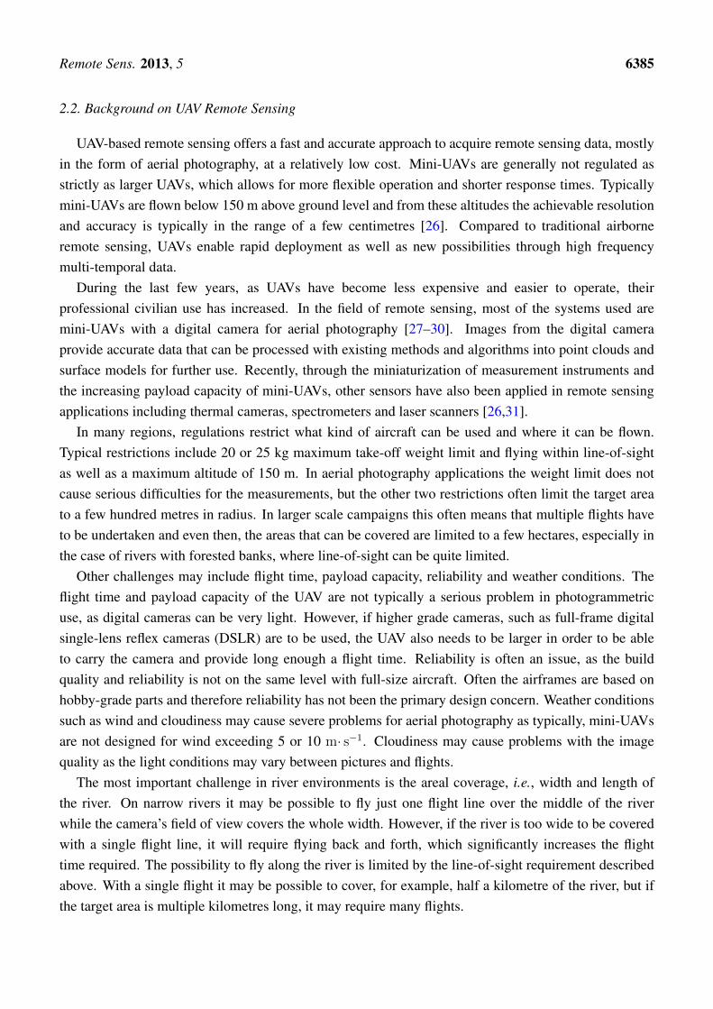
UAV-based remote sensing offers a fast and accurate approach to acquire remote sensing data, mostlyin the form of aerial photography, at a relatively low cost. Mini-UAVs are generally not regulated asstrictly as larger UAVs, which allows for more flexible operation and shorter response times. Typicallymini-UAVs are flown below 150 m above ground level and from these altitudes the achievable resolutionand accuracy is typically in the range of a few centimetres [26]. Compared to traditional airborneremote sensing, UAVs enable rapid deployment as well as new possibilities through high frequencymulti-temporal data.

During the last few years, as UAVs have become less expensive and easier to operate, theirprofessional civilian use has increased. In the field of remote sensing, most of the systems used aremini-UAVs with a digital camera for aerial photography [27–30]. Images from the digital cameraprovide accurate data that can be processed with existing methods and algorithms into point clouds andsurface models for further use. Recently, through the miniaturization of measurement instruments andthe increasing payload capacity of mini-UAVs, other sensors have also been applied in remote sensingapplications including thermal cameras, spectrometers and laser scanners [26,31].

In many regions, regulations restrict what kind of aircraft can be used and where it can be flown.Typical restrictions include 20 or 25 kg maximum take-off weight limit and flying within line-of-sightas well as a maximum altitude of 150 m. In aerial photography applications the weight limit does notcause serious difficulties for the measurements, but the other two restrictions often limit the target areato a few hundred metres in radius. In larger scale campaigns this often means that multiple flights haveto be undertaken and even then, the areas that can be covered are limited to a few hectares, especially inthe case of rivers with forested banks, where line-of-sight can be quite limited.

Other challenges may include flight time, payload capacity, reliability and weather conditions. Theflight time and payload capacity of the UAV are not typically a serious problem in photogrammetricuse, as digital cameras can be very light. However, if higher grade cameras, such as full-frame digitalsingle-lens reflex cameras (DSLR) are to be used, the UAV also needs to be larger in order to be ableto carry the camera and provide long enough a flight time. Reliability is often an issue, as the buildquality and reliability is not on the same level with full-size aircraft. Often the airframes are based onhobby-grade parts and therefore reliability has not been the primary design concern. Weather conditionssuch as wind and cloudiness may cause severe problems for aerial photography as typically, mini-UAVsare not designed for wind exceeding 5 or 10 m· s−1. Cloudiness may cause problems with the imagequality as the light conditions may vary between pictures and flights.

The most important challenge in river environments is the areal coverage, i.e., width and length ofthe river. On narrow rivers it may be possible to fly just one flight line over the middle of the riverwhile the camera’s field of view covers the whole width. However, if the river is too wide to be coveredwith a single flight line, it will require flying back and forth, which significantly increases the flighttime required. The possibility to fly along the river is limited by the line-of-sight requirement describedabove. With a single flight it may be possible to cover, for example, half a kilometre of the river, but ifthe target area is multiple kilometres long, it may require many flights.


2.3. Background on Optical Bathymetric Modelling in Rivers

The biggest challenge in mapping river environments lies in creating an accurate and continuousrepresentation of the submerged river bed itself. While small reaches of shallow rivers can be surveyedusing tachymetry [32] or a pole-mounted Real Time Kinematic Global Navigation Satellite System(RTK-GNSS), the limits of these methods are reached fairly quickly as the size of the area to be surveyedor the water depth increases. Furthermore, the accuracy of the terrain model that can be created basedon points surveyed in this fashion depends largely on the density of the point pattern, which is directlyproportional to time spent surveying. On the one hand, the positional accuracy of the points measuredusing tachymetry or RTK-GNSS can hardly be surpassed by other measuring techniques, but on the otherhand, remote sensing methods can provide much wider and more homogeneous spatial coverage.

The most widely used method for mapping underwater topography is sonar (e.g., [33]). Bothsingle-beam and multi-beam or swathe sonar can be used in rivers. While the coverage and density ofsingle-beam sonar points has the same limitations as the above-mentioned direct measurement methods,the method is much faster to apply and not limited to shallow water only. On the contrary, sonar systemsgenerally have minimum depth requirements of around 1 m in order for them to work [5]. Due to theirside-oriented sensors, swathe-sonar such as the Kemijoki Aquatic Technology AquaticSonar system [34]is able to measure shallow water near the river banks and measures a vastly higher point density. Sucha system measures a transect at a time and the gap between transects depends on the travel speed of theboat. However, even though shallow areas can be measured at a distance, the system is also dependenton the water being deep enough to deploy the boat, a limit which can be quickly reached in natural riversand streams. Measurements may therefore be limited to flood periods. Furthermore, the field of viewof side-scanning sonar systems increases with water depth, and conversely narrows to the point of beingunable to cover the river bed in shallow rives. In order to cover the whole river bed and to avoid possibleshadowing by islands, it is likely necessary to conduct multiple passes [35], and this need increases withdecreasing water depth.

Airborne remote sensing methods allow us to map larger areas of rivers contiguously and withoutminimum depth requirements. Airborne bathymetric mapping methods derive depth either based on thereturn time of an actively emitted light beam, in the case of green LiDAR, or on the spectral propertiesof recorded solar light, in the case of aerial photography based bathymetry [36]. Because these methodsrely on light penetration in the water column, they are dependent on reasonably low turbidity.

While green LiDAR is not yet used much for measuring river bathymetry [37], river bed topographyhas been mapped successfully using aerial photography using linear transform [38–41] or band ratiotransform methods [42–45]. The most commonly used method is the deep-water correction algorithmdeveloped by Lyzenga [9]. The method uses deep-water radiance in order to isolate the depth signalof the radiance recorded in an aerial or satellite image. Subtracting the radiance of an image pixelcontaining water deep enough for the river bed not to be visible from the image gives a value X ,the natural logarithm of which is linearly related to depth, thus allowing a simple regression modelto be established between these Lyzenga X values and measured reference depth points. Flener [46] hasrecently presented an algorithm for estimating this deep water radiance value in shallow rivers where itcannot be retrieved from the images otherwise, allowing the use of Lyzenga’s model in shallow rivers


where it performs best. Optically based bathymetric models reach their limit at a depth level where theradiance of the image bands used for modelling gets saturated, and therefore no longer changes withdepth [47]. This situation can occur at depths shallower than Secchi depth because most natural riverbeds are not pure white, so they reflect less light than a Secchi disc [46].

River researchers employing photography based bathymetry modelling have mostly focused on aerialphotography, because the higher spatial resolution that can be achieved this way suits the scale of analysisbetter than coarser satellite data. However, high resolution satellite data has recently also been used tomap gravel bed rivers in Wyoming, USA [48].

Aerial imagery based bathymetry models of rivers allow mapping river bed topography at scaleswider than the reach scale. Unlike methods that are based on point measurements, these models arebased on raster input data and therefore do not require interpolation of any kind to achieve a surfacemodel. Each image pixel is converted directly into a depth value. This spatial contiguity offsets thepossibly lower vertical accuracy that can be achieved with some of the other methods mentioned above.

Aerial imagery based bathymetric models rely on the river bed being visible, so that depth can bemodelled (e.g., [44]). This means that the water has to be reasonably clear, the water surface has to becalm enough so as to avoid ripples that cause bi-directional reflectance problems, and the view of theriver has to be unobstructed by overhanging trees, for instance.

In this study we employ the Lyzenga [9] algorithm combined with Flener’s [46] deep water estimationand apply it to high resolution photographs that were acquired using an unmanned aerial vehicle (UAV).

3. Study Area

The test area for all models is a meander bend of the river Pulmanki, located in northernmostFinnish Lapland (69◦56’N, 28◦2’E). The river Pulmanki flows in a valley of glaciofluvial deposits fromthe last glaciation, surrounded by fells. The river is about 20–30 m wide during summer low flow,depending on the water level, and the riverbed consists of sandy sediments. Kasvi et al. [18] andAlho and Mäkinen [49] describe the geomorphology of this study site in great detail. The typicaldischarges of the river Pulmanki vary between about 4 m3· s−1 during summer low flow and 40 m3· s−1

during the annual snow-melt induced spring flood. The water level can be two to four metres higherduring flood time than during summer low flow, depending on the size of the flood. This flow regimecombined with the unstable sediments make this a very dynamic river [50] that is ideal for changedetection studies.

4. Data Collection

In this study we combine a range of measurement methods that allow us to create high resolutiontopographic data of the study area. We use the ROAMER mobile mapping system (MMS) developed bythe Finnish Geodetic Institute (FGI), which can be applied both as a boat based mobile mapping system(BoMMMS) [24,51] and cart/backpack-based MMS (Akhka) [52]. To the best of our knowledge, thisis the most advanced mobile laser scanning platform currently employed in fluvial studies. We combinethese scanning methods with low-altitude aerial photography we gather using an unmanned aerial vehicle(UAV). We use these images to create both an image-based bathymetric model of the river bed and


a photogrammetry-based point cloud of the study area. All methods were applied during two fieldcampaigns, during the end of August and early September 2010 and 2011. During this time of theyear, the water levels of the rivers in this area of the sub-arctic are usually at their lowest. This allowedus to scan a large part of the channel using LiDAR. Furthermore, this maximised the chances of thebathymetric modelling being successful due to low turbidity and low water levels, minimising the risk ofthe deeper parts of the channel exceeding attenuation depth. During our field campaigns, the water depthin the study area did not exceed 1.5 m. Turbidity outside of the spring flood is extremely low, meaningthat the whole river bed was visible from the air.

4.1. LiDAR

Table 1 gives an overview of the laser scanners, IMU and GPS navigation equipment we used duringthe different field campaigns. We used a Leica HDS6100 scanner in stationary mode (TLS) and FaroPhoton 120 scanner mounted on mobile scanning platforms for the mobile mapping system setups.

Table 1. Laser scanning systems used. We used two different scanners, one deployed on astationary platform and one deployed on three different mobile scanning platforms.

Date ScannerScanning Point Sensor Height Navigation System

AngularFrequency Frequency Resolution

(Hz) (kHz) (m) (◦)

TLS2010 Leica HDS6100 25 213 2 n/a 0.0362011 Leica HDS6100 25 213 2 n/a 0.036

BOMMS2010 31.8. Faro Photon 120 49 244 2.5 NovAtel SPAN GPS-IMU 0.0722011 8.9. Faro Photon 120 49 244 2.5 NovAtel SPAN GPS-IMU 0.072

CartMMS2010 31.8. Faro Photon 120 49 244 2.3 NovAtel SPAN GPS-IMU 0.072

AkhkaMMS2011 9.9. Faro Photon 120 49 244 1.9 NovAtel SPAN GPS-IMU 0.072

4.1.1. MLS Field Measurements (2010–2011)

The MLS systems we used consisted of a Faro Photon 120 laser scanner and NovAtel SPANnavigation system with NovAtel DL4plus GPS receiver, NovAtel 702 GPS antenna and HoneywellHG1700 AG58 inertial measurement unit. In the ROAMER system these instruments are integratedinto a platform with an adjustable scanning angle, designed at FGI. In 2010 we operated the ROAMERMLS system on a boat to collect laser scanning data of the point bar shoreline and the steep banks.We collected data of other parts of the point bars using ROAMER installed on top of a cart. In 2011ROAMER was again set up on a boat, but we mapped the point bars using the Akhka backpack MLSsystem. In Akhka the measurement instruments are installed on a compact and rigid platform, which isattached to the frame of a backpack. Figure 1 shows the different setups of the ROAMER system. Inall cases the scanning frequency was set to 49 profiles per second and the point measurement frequencywas 244,000 points per second. The profile spacing was 2–3 cm at an average speed of 4 km/h. Thescanner field-of-view is 320 degrees, which means that, in case of the boat installation, no data was


acquired below the scanner (boat) and in case of the cart and backpack installations, above the scanner(sky). The BoMMS and CartMMS measurements produced a 200 m trajectory that took three minutesto measure in each case. The Akhka trajectory was 350 m long and took 4.5 min to measure in the field.We used spherical reference targets for orienting the scans to the coordinate system. We used five targetsin 2010 and four targets in 2011. The location of each reference target was measured using an RTK-GPSand can be seen in Figures 2 and 3.

Figure 1. Different setups for the FGI ROAMER mobile mapping system: BoMMS (left);CartMMS (centre); Akhka (right).

Figure 2. Moble LiDAR point cloud of 2010 (left) and TLS reference point cloud 2010(right) coloured by elevation.


Figure 3. Mobile LiDAR point cloud of 2011 (left) and TLS reference point cloud 2011(right) coloured by elevation.

We enabled the Clear Contour and Clear Sky hardware filtering provided by the scanner unit in theMLS data collection on-the-fly to reduce measurement noise, especially from the sky. The Clear Contourfilter removes incorrect measurements at the edges of objects by removing scan points resulting fromhitting two objects with the laser spot, which mainly happens at the edges of objects. The Clear Skyhardware filter removes scan points resulting from hitting no objects at all, which mainly happens whenscanning the sky.

4.1.2. MLS Data Processing

During preprocessing, dark points with an intensity value of less than 800 (the full range being 11 bit,0–2,047) were removed to further reduce weak returns from objects. Then, below ground surface noisewas partially removed manually to avoid problems with ground classification by removing all pointswith an elevation lower than the water surface elevation.

We classified the MLS point cloud datasets based on the principles of Axelsson [53]. The methodtakes three parameters: terrain angle, limiting the maximum slope of the surface to be created; iterationangle, the maximum angle between a point, its projection on the triangulated plane along the trianglenormal, and the closest triangle vertex; and iteration distance, limiting vertical jumps that can occur withlarge triangles. The smaller the iteration angle, the less eager the routine is to follow changes in the pointcloud (small undulations in terrain or hits on low vegetation). We used an 88 degree terrain angle, a 25degree iteration angle and a 20 cm iteration distance for the classification of the ground points of the pointbar in question. We processed all the MLS data from BoMMS for both years 2010 and 2011, CartMMSfor 2010 and Akhka for 2011 using the same parameters with a few manually pointed ground points oneach to start the ground classification iteration. The ground classification with the selected parametervalues succeeded in removing vegetation from the edge of the point bar and the opposing bank.

In order to create a DTM suitable for analysis, it is necessary to reduce the vast amount of pointsmeasured by the MLS. In the first step, we combined the ground data from different MLS sources intotwo point sets, one for each year.


The next step differed slightly for the two datasets as the 2010 ground data was reduced directly usingmodel keypoint thinning [54]. Due to the very large data size of the 2011 data set, it was first averagedto a 5 cm grid and reduction was carried out with a thinning method allowing a 1 cm elevation differencetolerance between local points, preserving the central points of a local group of points. As a result, wegenerated two MLS DTMs for the point bar to be combined with the UAV bathymetry DTMs. The 2010DTM consisted of 2.1 million 3D points with an average density of 140 pts/m2. The 2011 DTM had1.7 million points with an average density of 70 pts/m2. Regarding the performance of the two thinningmethods applied, the result is expected to be equal for both data sets because the point density of theoriginal data is stupendous combined with millimetre scale ranging precision, and due to the selectedground distance of 5 cm. Figures 2 and 3 show the MLS point clouds for 2010 and 2011 respectivelynext to the TLS point clouds used for their evaluation.

4.1.3. TLS Field Measurements (2010–2011)

We used a Leica HDS6100 laser scanner to acquire terrestrial laser scanning data to use as referencedata of the study area during both field campaigns. The TLS measurements and the installation ofreference targets of the study area took 30 min. The point bar area was scanned with a 360◦ horizontalfield of view (FOV) and a resolution that produced a point spacing of 6 mm at a 10 m distance fromthe scanner. We conducted two scans in 2010 and four scans in 2011 using the same sphere referencetargets as for MMS for orientation of the scans to the coordinate system. The location of each referencetarget was measured using an RTK-GPS. The achievable accuracy of the RTK-GPS measurements is1 cm + 1–2 ppm horizontally and 1.5–2 cm + 2 ppm vertically (RMSE) [55]. The final accuracy of theTLS point cloud is on the same level as that of the RTK-GPS-measured target spheres.

The TLS data was classified using the same method as the MLS data using the method developed byAxelsson [53]: the maximum ground surface inclination was set to 88◦, the maximum iteration anglewas 25◦ to the triangular surface between these points and a maximum allowable difference of 20 cm toalready triangulated surfaces. The parameters were chosen to suit the data set, taking into considerationterrain slope, roughness and point density. After the ground classification, every hundredth point wasused for the comparison to the MLS data (cf. Figures 2 and 3).

4.2. UAV Photography

4.2.1. UAV Field Measurements (2010–2011)

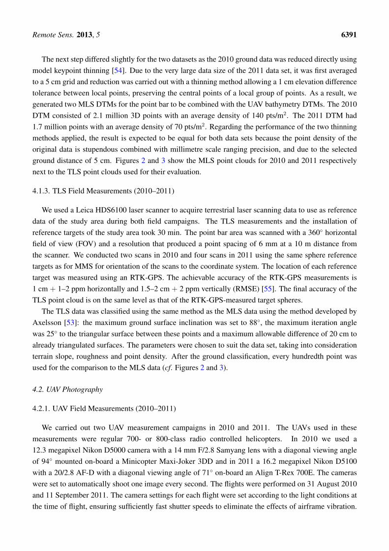
We carried out two UAV measurement campaigns in 2010 and 2011. The UAVs used in thesemeasurements were regular 700- or 800-class radio controlled helicopters. In 2010 we used a12.3 megapixel Nikon D5000 camera with a 14 mm F/2.8 Samyang lens with a diagonal viewing angleof 94◦ mounted on-board a Minicopter Maxi-Joker 3DD and in 2011 a 16.2 megapixel Nikon D5100with a 20/2.8 AF-D with a diagonal viewing angle of 71◦ on-board an Align T-Rex 700E. The cameraswere set to automatically shoot one image every second. The flights were performed on 31 August 2010and 11 September 2011. The camera settings for each flight were set according to the light conditions atthe time of flight, ensuring sufficiently fast shutter speeds to eliminate the effects of airframe vibration.


Focus was set to manual and locked at infinity. The weather conditions during 2010 were bright, slightlyovercast and the camera was set to 1/4,000s, F/5.6, ISO 800. During the 2011 flight conditions weremore overcast and the camera was set to 1/1,000s, F/5.6, ISO 800. In 2010, the flight duration was threemin and the minimum, mean and maximum flight heights above ground were 58 m, 71.3 m and 86.8 mrespectively. In 2011, the total flight time was six min and the minimum, mean and maximum flightheights above ground were 79.6 m, 127.5 m and 145.1 m. Ground control target points (GCP) made of60 × 60 cm plywood with high contrast paint and a precise centre point were located along the riverreaches under survey in fairly regular intervals. The points (3 in 2020, 5 in 2011) were surveyed usinga RTK-GNSS.

The most challenging aspects of the UAV measurements were coverage and UAV reliability. Becausethe UAV was manually controlled and there was no real-time feedback on the location or image coverageof the UAV, some of the areas were not covered sufficiently to be reconstructed for later analysis.Also the reliability of the aerial vehicles caused problems; in 2010 one the UAVs had a malfunctionand ended up falling into the river being measured. This is the reason why the UAV and the cameramodel were changed between the campaigns.

4.2.2. UAV Image Processing (2010–2011)

The images of all flights were evaluated for image quality. Quality issues relate mostly to reflectionof the sky on the water surface and illumination changes during the time of the flights. There were noclouds reflecting on the water surface but there was some effect of sunlight illumination changing duringflight time. Based on these quality considerations, a subset of suitable images was chosen to create thefinal image mosaics.

In 2010, 185 images were captured during the three-minute flight. Due to the camera shooting animage every second during the entire flight, most of these images were captured during take-off andlanding, which is the slowest part of the flight. 41 images were used for further processing, selected formaximising areal coverage, image overlap and image quality. In 2011, 27 out of a total of 213 imagescaptured were used for processing.

All the selected images were converted from RAW to TIFF with the white-balance set to flashmode and +0.5 exposure boost. Lens distortion was removed and the images were centred on the realoptical centre of the lens using Matlab, based on a set of calibration images shot in the field prior toeach flight. An initial estimate of exterior orientation was calculated by manually collecting commontarget points from overlapping images using the iWitness photogrammetry software. The orientationwas then improved using the aerial triangulation functions in BAE Systems’ Socet Set software, whichautomatically finds similar features in the images, creating a denser common point network.

The mosaics were projected to the elevation of the water level of the river using the GNSS-measuredground control points and exported as GeoTIFF (Figure 4). Using GCP:s as a benchmark both imageshave under 10 cm positional errors in XYZ. The image resolution on the ground varies between a fewmm up to 20 cm at its worst. The final image mosaics were sampled to a 5 cm GSD (ground sampledistance) in Socet Set.

The photogrammetry point clouds produced based on the distortion-corrected images using Autodesk123D were georeferenced to the GCPs (Figure 5).


Figure 4. UAV image mosaics of 2010 (left) and 2011 (right). Both images are RGB at0.05 m ground sample distance. The distortion notable outside the river bed stems form theimage distortion at the edges of the frames in combination with the planar rectification of themosaic to the water level of the river.

Figure 5. UAV photogrammetry-derived point cloud of 2010 (left) and 2011 (right)coloured by elevation.

4.3. UAV-Bathymery Modelling

4.3.1. Ground Data Measurements (2010–2011)

In 2010, 197 river bed elevation points were measured using an RTK-GPS. These points wereconverted to depth data by subtracting the elevation from an interpolated water surface, also based onRTK-GPS points. This depth data is required for calibrating the optical bathymetric model.


In order to gather more points for analysis, in 2011 we used a remote controlled boat with a SontekRiverSurveyor M9 ADCP on board to measure water depth points directly, as well as water surfacepoints. An RTK-GPS was mounted on the boat in addition to the Sontek DGPS in order to get accuratelocation data for the depth measurements. The sonar of the Sontek M9 measures depths >0.18 m withan accuracy of 2.5% of the depth and saves measurements at 1 s intervals. The ADCP-measured depthpoints were merged with the RTK-GPS data by combining the time stamps of the two GPS devices.

Figure 6. Bathymetric models of 2010 (left) and 2011 (right) using the Lyzenga model withcalibrated Lsi values. The plots show the modelled depths vs. the measured depths at theground data reference points. Green areas were modelled as dry (i.e., negative depths).

-0.5 0.0 0.5 1.0 1.5

-0.5

0.0

0.5

1.0

1.5

measured Depth (m)

mod

elle

d D

epth

(m)

-1 0 1 2

-1

0

1

2

measured Depth (m)

mod

elle

d D

epth

(m)

4.3.2. Building the Bathymetry DSM

We built the bathymetric models as rasters based on the image mosaics produced from the UAVimages. The models were calculated using Lyzenga’s [9] model. Since none of the area to be modelledexceeded Secchi depth we estimated deep water radiance values according to the method developed byFlener [46]. The depth models as well as their deep water radiance parameters were calibrated using


100-fold random sub-sampling cross-validation with a 70% training set and 30% test set. The means ofthe cross-validation output were used to determine the regression coefficients needed to build the depthmodel and the mean of the accuracy statistics of all cross-validation runs were used to determine modelaccuracy. The image-based model produces a bathymetry raster that has the same spatial properties asthe image raster did, in this case a grid with a ground resolution of 0.05 m (Figure 6). The bathymetryraster was finally converted to elevation values by subtracting the depth values form an interpolatedwater surface. For the 2010 model, this surface was based on two water level points measured at theshoreline, while for the 2011 model, the water surface was based on an interpolation of the water levelpoints measured by the ADCP–RTK-GPS setup. In order to facilitate combining the bathymetry datawith the LiDAR data, the raster was converted to regularly spaced 3D point data.

5. Accuracy Assessment

We evaluated the different models against measured reference data in order to assess their accuracy:we used the TLS point cloud as reference data on the dry part of our study area and the GPS based riverbed elevation points as the primary reference for the submerged riverbed. The TLS point cloud is thehighest quality representation of the land surface that is available [56], being of the same level of accuracyas the RTK-GPS measured target points used for its georectification. Figures 2 and 3 show the mobilelaser scanning point clouds and the TLS data used as reference for the 2010 and 2011 measurementcampaigns respectively.

Table 2. Accuracy assessment of the seamless model using TLS as reference data on the drypart of the point bar and measured depth points in the submerged part of the river channel.The bathymetry cross-validation accuracy data is included here for comparison to the finalseamless model results, where depth has been converted to elevation. The average magnitudeindicates the average absolute elevation difference and the dz values denote the minimum andmaximum elevation differences between the compared data sets. All values are in metres.

Data Set Reference Data Vertical Average RMSE min dz max dzAdjustment Magnitude

Point bar dataMLS (BoMMS + CartMMS) 2010 TLS points on pointbar 0.01 0.0103 0.0151 −1.1020 +0.4920MLS (BOMMS + Akhka) 2011 TLS points on pointbar 0.01 0.0136 0.0182 −0.8730 +0.1210

UAV-point-cloud 2010 TLS points on pointbar 0.03 0.0900 0.1520 −0.3970 +4.3640UAV-point cloud 2011 TLS points on pointbar 0.5 0.0705 0.088 −0.7100 +0.4990Riverbed dataUAV-bathymetry 2010 Cross-validation n/a 0.097UAV-bathymetry 2010 RTK-GPS points 0.12 0.1196 0.221 −1.3503 +1.3562UAV-bathymetry 2011 Cross-validation n/a 0.078UAV-bathymetry 2011 ADCP–RTK-GPS points −0.50 0.117 0.163 −1.015 +0.460

We used the TerraScan software package to evaluate the different point clouds against each other. Thisinvolves calculating locally triangulated surface models around each reference point using the closestmeasured points and calculating the elevation difference between the reference point to the same xy


coordinate on the model surface. Table 2 summarises these accuracy assessments along with the accuracyassessment based on the cross-validation of the bathymetric model.

Mobile laser scanning clearly delivers the most accurate data, with an RMS error of under 2 cmcompared to the TLS data. Figure 7A shows that the mobile laser data is in very good agreement withthe TLS reference data.

Figure 7. Elevation points of MLS vs. TLS models (A) and UAV photogrammetry vs. TLS(B) of 2010 (left) and 2011 (right).

The bathymetric models deliver fairly accurate depth data with RMSE varying between 8 and 10 cmin cross-validation of modelled and measured depths. When looking at the elevation data of the river bed(rather than depth data) relative to RTK-GNSS-measured elevations, the error doubles.

The UAV photogrammetry data vary in accuracy between the two years. The 2011 point cloud, withan RMSE of 0.088, is about twice as accurate as the one produced form the 2010 images. The pointcloud of 2010 covers a smaller area and includes some areas on the pointbar area that exhibit low pointdensity due to low contrast, making it difficult for the algorithms to locate common points in differentpictures, causing the overall error to be larger. The 2010 image network was less constant than thatof 2011, causing limited image overlap in some areas, due to a more varying flight height and pattern.The 2011 flight was at a slightly higher and more constant altitude with a more consistent flight pattern,


leading to a better photogrammetric result. Figure 7 (2010 B) shows that, while the spread of points islarger than that of the MLS data, the errors are concentrated at the higher elevations, which is where theartefacts are located on the sandbank.

6. Building the Seamless DTM

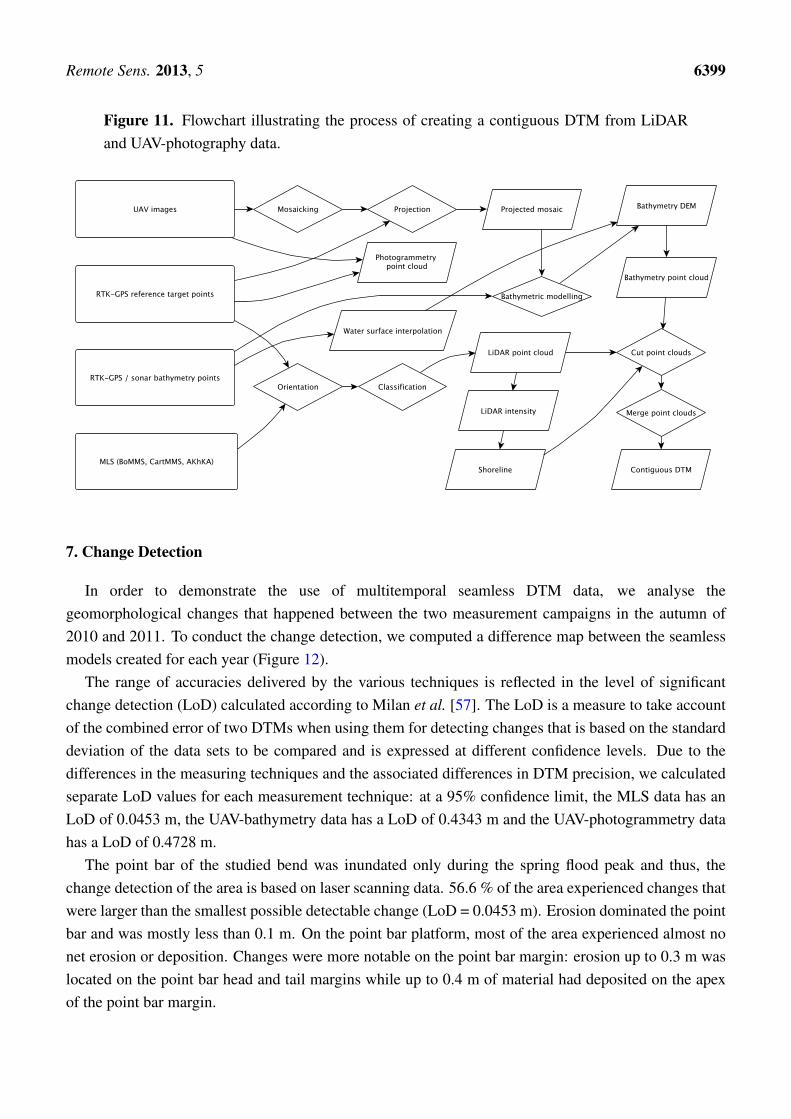
We produced the seamless terrain model of the meander bend by combining the MLS data (BoMMS+ CartMMS in 2010; BoMMS + Akhka in 2011) for the dry area of the point bar with the bathymetrymodel created from the UAV pictures. Based on the results of the accuracy analysis of all data sets, thisgives us the pest possible seamless DTM. The data sets contained some overlapping areas because thevery clear water allowed the BoMMS data to also include some bathymetry points near the shoreline(the system used a 785 nm wavelength laser beam), while the bathymetric model also included some dryareas. Milan et al. [57] had also found that the signal of a red TLS can penetrate water, although theyfound the accuracy to decrease with increasing depth. Vaaja et al. [51] found a clear change in intensityvalues at the border of submerged and non-submerged terrain. This change in intensity is visualisedin Figure 8. Vetter et al. [5] also delineated the water surface area of a river using the intensity ofALS returns. Based on this observation, we separated these areas by digitizing the shoreline accordingto the BoMMS intensity data. Because the positional accuracy of the underwater BOMMS points isunknown, due to light refraction at the water surface, especially at the relatively shallow scanning angle,we deleted these points from contiguous model using the extracted shoreline. The UAV-imagery-basedbathymetry point data was used exclusively for the underwater part of the channel. Figure 9 showsthe contiguous model created by combining the point cloud data of the MLS and the UAV-bathymetry.Figure 10 shows two transects for each year through the whole model, including the dry pointbar and theriverbed. The transect line locations are shown in Figure 9. Figure 11 illustrates the entire processingchain required to produce the contiguous DEM from mobile LiDAR data and bathymetry data createdfrom UAV-photography.

Figure 8. Map of the BoMMS intensity data of 2010 (left) and 2011 (right) used todetermine the shoreline (marked in red). The intensity change at the edge between inundatedand non-inundated river bed that is used in the digitization of the shoreline is clearly visiblein the scatterplot of the transect marked in green.


Figure 9. Seamless digital elevation model of 2010 and 2011 combining mobile laserscanning data with the UAV-based bathymetry as a 3D point cloud coloured by elevation.The lines indicate the transects shown in Figure 10.

Figure 10. Transects of elevation data indicating the seamless merging of the MLS data withthe bathymetry data. The location of the transects is indicated in Figure 9.


Figure 11. Flowchart illustrating the process of creating a contiguous DTM from LiDARand UAV-photography data.

7. Change Detection

In order to demonstrate the use of multitemporal seamless DTM data, we analyse thegeomorphological changes that happened between the two measurement campaigns in the autumn of2010 and 2011. To conduct the change detection, we computed a difference map between the seamlessmodels created for each year (Figure 12).

The range of accuracies delivered by the various techniques is reflected in the level of significantchange detection (LoD) calculated according to Milan et al. [57]. The LoD is a measure to take accountof the combined error of two DTMs when using them for detecting changes that is based on the standarddeviation of the data sets to be compared and is expressed at different confidence levels. Due to thedifferences in the measuring techniques and the associated differences in DTM precision, we calculatedseparate LoD values for each measurement technique: at a 95% confidence limit, the MLS data has anLoD of 0.0453 m, the UAV-bathymetry data has a LoD of 0.4343 m and the UAV-photogrammetry datahas a LoD of 0.4728 m.

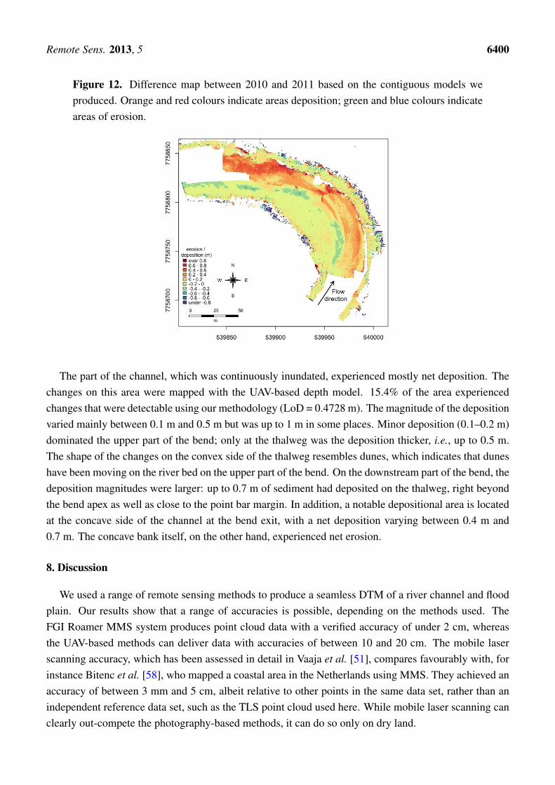
The point bar of the studied bend was inundated only during the spring flood peak and thus, thechange detection of the area is based on laser scanning data. 56.6 % of the area experienced changes thatwere larger than the smallest possible detectable change (LoD = 0.0453 m). Erosion dominated the pointbar and was mostly less than 0.1 m. On the point bar platform, most of the area experienced almost nonet erosion or deposition. Changes were more notable on the point bar margin: erosion up to 0.3 m waslocated on the point bar head and tail margins while up to 0.4 m of material had deposited on the apexof the point bar margin.


Figure 12. Difference map between 2010 and 2011 based on the contiguous models weproduced. Orange and red colours indicate areas deposition; green and blue colours indicateareas of erosion.

The part of the channel, which was continuously inundated, experienced mostly net deposition. Thechanges on this area were mapped with the UAV-based depth model. 15.4% of the area experiencedchanges that were detectable using our methodology (LoD = 0.4728 m). The magnitude of the depositionvaried mainly between 0.1 m and 0.5 m but was up to 1 m in some places. Minor deposition (0.1–0.2 m)dominated the upper part of the bend; only at the thalweg was the deposition thicker, i.e., up to 0.5 m.The shape of the changes on the convex side of the thalweg resembles dunes, which indicates that duneshave been moving on the river bed on the upper part of the bend. On the downstream part of the bend, thedeposition magnitudes were larger: up to 0.7 m of sediment had deposited on the thalweg, right beyondthe bend apex as well as close to the point bar margin. In addition, a notable depositional area is locatedat the concave side of the channel at the bend exit, with a net deposition varying between 0.4 m and0.7 m. The concave bank itself, on the other hand, experienced net erosion.

8. Discussion

We used a range of remote sensing methods to produce a seamless DTM of a river channel and floodplain. Our results show that a range of accuracies is possible, depending on the methods used. TheFGI Roamer MMS system produces point cloud data with a verified accuracy of under 2 cm, whereasthe UAV-based methods can deliver data with accuracies of between 10 and 20 cm. The mobile laserscanning accuracy, which has been assessed in detail in Vaaja et al. [51], compares favourably with, forinstance Bitenc et al. [58], who mapped a coastal area in the Netherlands using MMS. They achieved anaccuracy of between 3 mm and 5 cm, albeit relative to other points in the same data set, rather than anindependent reference data set, such as the TLS point cloud used here. While mobile laser scanning canclearly out-compete the photography-based methods, it can do so only on dry land.


The UAV-photography-bathymetry model was able to deliver depth accuracies of under 10 cm, but theaccuracy decreases when comparing the depths that were converted to elevation to the RTK-GNSS data.Previous studies using optical imagery-based bathymetry assessed the bathymetric data against otherdepth data, rather than bathymetry converted to elevation data (e.g., [40,41,45,59,60]). The decrease inaccuracy when comparing under-water elevations to RTK-GNSS-measured elevations, is likely due toimprecision in the water surface model used to convert the depth values to elevation values. In 2010in particular, the water surface was calculated as a theoretical surface based on RTK-GPS–measuredshoreline points and does not represent the real water surface as accurately as the one created formthe ADCP–RTK-GPS–measured water surface points. This model was used both to convert the GPSpoints to depth, so that the bathymetric model could be calibrated, and subsequently to convert thebathymetric model to an elevation model. In 2011 the depth points had been measured directly so thewater surface model was only used at one point in the procedure, to convert the bathymetric model to anelevation model. Moreover this surface was interpolated form the water surface points measured with theRTK-GPS embarked on the ADCP. This indicates that the bathymetric model is able to produce depthestimates well, but that the water surface model used to convert the elevations to depth and the depths toelevations is of great importance when creating a DTM from a bathymetric model. Williams et al. [6]analysed the effect of different methods of water surface interpolations on the accuracy of bathymetryderived elevations and found errors in water surface models to propagate to the bed elevations derivedfrom optical bathymetric modelling. Considering the result of the bathymetry-based DEM, the accuracyis in line with most sonar systems, while, unlike sonar, providing a raster model that does not requireinterpolation to create the DEM, thereby delivering spatially continuous data.

The UAV-based photogrammetry point data covers the dry and the submerged river channel. However,the refraction of light at the water surface is not taken into account in the creation of the photogrammetrypoint cloud, therefore the positional accuracy of the submerged points is unknown. We consider the UAVphotogrammetry data only for the dry area in this study. The accuracy delivered by this method can befairly good (sub-decimetre) but the difference in accuracy between the two flight campaigns shows that itdepends on the image data. One important factor here is the number of images that can be used to createthe model, and the geometric quality of the image network, that is, the relative positions of the imageorigins over the target area. Other factors that affect the accuracy of UAV-photogrammetry point cloudsare image lens abberations and distortions and image sharpness. The 2010 images were shot using a14 mm lens from a lower altitude and at lower resolution, leading to more distortion and less ability forthe algorithm to distinguish common features in multiple images, especially on the rather low-contrastsandbank. In comparison, the 2011 images were shot from a higher altitude using a 20 mm lens, leadingto less distortion that needs correcting, and at a higher resolution allowing to detect common pointseasier even in low-contrast areas, leading to better results. The difference in accuracy can be clearly seenin Figure 5. The 2010 point cloud shows some geometric shapes on the point bar which is reflected inthe scatter plot in Figure 7 by a drastic spread of points at the higher end of the elevation spectrum.

When creating a seamless wet-dry DTM, the best result can be achieved by combining high-accuracyMLS data for the dry part with UAV-photography based bathymetric modelling. This does require a suiteof expensive equipment, though, so depending on the intended use of the DTM, a UAV-only solution maybe preferable, combining photogrammetry point clouds for the dry areas with bathymetric modelling


for the inundated part. Given a large number of high-quality images shot from a relatively constantheight and clear water conditions with uniform sediment and illumination throughout the scene, bothwet and dry areas can be modelled at high resolution with around 10 cm vertical accuracy using theUAV-photography based methods we applied in this study. This level of accuracy should be satisfactoryfor many applications such as hydraulic modelling or habitat studies [13]. However, when the objectiveis to study small geomorphic features such as the dynamics of sand dunes and ripples in natural riverenvironments, the extra level of accuracy delivered by mobile laser scanning [61–63] or terrestrial laserscanning [6,13,64] is required. Such detailed riverine processes have thus far not been studied muchoutside laboratory flumes, due to the previous difficulty of obtaining data that is accurate enough for thispurpose in natural rivers. The combination of MMS and UAV-based high-resolution bathymetry makesdetailed studies of river dynamics possible in natural environments.

The change detection in the present study reveals that, even though the seamless model is able to givea synoptic view of the river channel, the difference in accuracy of the measurement methods needs tobe taken into account when analysing changes in detail. The high accuracy of the MMS measurementsallows us to detect smaller (sub-decimetre) changes on the dry part of the channel than can be achieved onthe inundated part of the channel, expressed as LoD (cf. Kasvi et al. [18]). Therefore, the interpretationof changes differentiates between both parts of the channel, all the while giving a more complete insightinto the erosion and deposition processes taking place than a more traditional study focussing on eitherpart of the channel alone would.

A detailed look at the coverage of the change detection map demonstrates that any lack of coveragein measurements accumulates over time and limits the change interpretation. Figure 12 shows that thepart of the channel that is inundated throughout the year experienced mostly deposition, but a narrowstrip of channel bed on the outside of the bend, including one slightly wider area, is missing form thismap because the UAV photography mosaic had a gap in this area in 2011. The narrow irregular stripof missing data is due to overhanging trees that made bathymetric modelling in that area impossible.Any missing areas accumulate and the map of changes can only cover those areas that are covered atall time steps. For this reason, methodological redundancy is desirable since it minimises the likelihoodof spatial gaps in the data. While such gaps may be tolerable to some extent in a single measurementcampaign, they are accentuated in multi-temporal studies, and should therefore be minimised as muchas possible. It may therefore be desirable to process and analyse the gathered data in the field as far aspossible in order to immediately recognise any gaps so that these can be filled with either a modifiedapproach of the same method, or, in case they are caused by obstructions, using other methods. In casethe view of the river bed from the UAV is obstructed by overhanging trees, the no-data areas this createsin the optical bathymetric model can be filled using sonar for instance.

9. Conclusions

This study has demonstrated the creation of seamless digital elevation models in river environmentsby combining mobile laser scanning with UAV-photography based bathymetry modelling. We concludethat a continuous wet–dry model of the river channel can be constructed at a sub-decimetre resolutionwith vertical accuracy within the same range. If the accuracy requirement is in the +/− decimetre scale,


we find that a UAV-only system, combining photogrammetry with optical bathymetry may be sufficient.When sub-decimetre accuracy is required, the combination of boat-based and backpack-based mobileLiDAR is the most efficient way of mapping river environments. TLS, used here as reference data, willmeet even centimetre scale accuracy requirements, however the aerial coverage is more limited in thatcase. The methods presented in this paper lend themselves well to mapping larger areas than the testarea covered in this study. The mobile LiDAR setup used here was for instance successfully employedin a study of lateral erosion of a 1.8 km stretch of river in Lotsari et al. [65]. From a logistical point ofview, both methods can be efficiently employed almost simultaneously in the field, making use of thesame ground target setups, thereby saving time and increasing efficiency.

Despite the contiguous data produced, the differences in measurement accuracy need to betaken into account when using these terrain models in a multi-temporal analysis of change. Thecombination of different high-resolution mobile remote sensing methods allows us to create seamlessDTMs of decimetre to centimetre accuracy and resolution that will support two- or three-dimensionalhydrodynamic modelling and fluvial geomorphological investigations.

Acknowledgments

This study was funded by the Academy of Finland (RivCHANGE research project), The AaltoEnergy Efficiency research programme (project Light Energy—Efficient and Safe Traffic Environments),Research on resident-driven infill development possibilities—case study in urban areas in Finland(REPSU) and the Geography Graduate School of Finland. Fieldwork was supported by the KevoSubarctic Research Station and the field assistance of Eliisa Lotsari is gratefully acknowledged.

Conflicts of Interest

The authors declare no conflict of interest.

References

1. Veijalainen, N.; Lotsari, E.; Alho, P.; Vehviläinen, B.; Käyhkö, J. National scale assessment ofclimate change impacts on flooding in Finland. J. Hydrol. 2010, 391, 333–350.

2. Lotsari, E.; Wainwright, D.; Corner, G.; Alho, P.; Käyhkö, J. Surveyed and modelled one-yearmorphodynamics in the braided lower Tana River. Hydrol. Process. 2013, doi:10.1002/hyp.9750.

3. Alho, P.; Hyyppä, H.; Hyyppä, J. Consequence of DTM precision for flood hazard mapping: Acase study in SW Finland. Nord. J. Surv. Real Estate Res. 2009, 6, 21–39.

4. Hicks, D.M.; Shankar, U.; Duncan, M.J.; Rebuffé, M.; Aberle, J. Use of Remote-Sensing withTwo-Dimensional Hydrodynamic Models to Assess Impacts of Hydro-Operations on a Large,Braided, Gravel-Bed River: Waitaki River, New Zealand. In Braided Rivers; Smith, G.H.S.,Best, J.L., Bristow, C.S., Petts, G.E., Eds.; Blackwell Publishing Ltd.: Malden, MA, USA 2009;pp. 311–326.


5. Vetter, M.; Hofle, B.; Mandlburger, G.; Rutzinger, M. Estimating changes of riverine landscapesand riverbeds by using airborne LiDAR data and river cross-sections. Z. Geomorphol. Suppl.Issues 2011, 55, 51–65.

6. Williams, R.; Brasington, J.; Vericat, D.; Hicks, D. Hyperscale terrain modelling of braided rivers:Fusing mobile terrestrial laser scanning and optical bathymetric mapping. Earth Surf. Process.Landf. 2013, doi:10.1002/esp.3437.

7. Allouis, T.; Bailly, J.S.; Feurer, D. Assessing Water Surface Effects on LiDAR BathymetryMeasurements in Very Shallow Rivers: A Theoretical Study. In Proceedings of the Second Spacefor Hydrology Workshop “Surface Water Storage and Runoff: Modeling, In-Situ Data and RemoteSensing”, Geneva, Switzerland, 12–14 November 2007.

8. Feurer, D.; Bailly, J.S.; Puech, C.; Le Coarer, Y.; Viau, A.A. Very-high-resolution mapping ofriver-immersed topography by remote sensing. Prog. Phys. Geogr. 2008, 32, 403–419.

9. Lyzenga, D.R. Remote sensing of bottom reflectance and water attenuation parameters in shallowwater using aircraft and Landsat data. Int. J. Remote Sens. 1981, 2, 71–82.

10. Best, J. The fluid dynamics of river dunes: A review and some future research directions.J. Geophys. Res. Earth Surf. 2005, 110, doi:10.1029/2004JF000218.

11. Fuller, I.C.; Large, A.R.; Charlton, M.E.; Heritage, G.L.; Milan, D.J. Reach-scale sedimenttransfers: An evaluation of two morphological budgeting approaches. Earth Surf. Process. Landf.2003, 28, 889–903.

12. Smith, M.J.; Chandler, J.; Rose, J. High spatial resolution data acquisition for the geosciences:Kite aerial photography. Earth Surf. Process. Landf. 2009, 34, 155–161.

13. Heritage, G.; Hetherington, D. Towards a protocol for laser scanning in fluvial geomorphology.Earth Surf. Process. Landf. 2007, 32, 66–74.

14. Cobby, D.M.; Mason, D.C.; Davenport, I.J. Image processing of airborne scanning laser altimetrydata for improved river flood modelling. ISPRS J. Photogramm. Remote Sens. 2001, 56, 121–138.

15. Bates, P. Remote sensing and flood inundation modelling. Hydrol. Process. 2004, 18, 2593–2597.16. Hyyppä, J.; Hyyppä, H.; Leckie, D.; Gougeon, F.; Yu, X.; Maltamo, M. Review of methods of

small-footprint airborne laser scanning for extracting forest inventory data in boreal forests. Int. J.Remote Sens. 2008, 29, 1339–1366.

17. Mason, D.C.; Cobby, D.M.; Horritt, M.S.; Bates, P.D. Floodplain friction parameterization intwo-dimensional river flood models using vegetation heights derived from airborne scanning laseraltimetry. Hydrol. Process. 2003, 17, 1711–1732.

18. Kasvi, E.; Vaaja, M.; Alho, P.; Hyyppä, H.; Hyyppä, J.; Kaartinen, H.; Kukko, A. Morphologicalchanges on meander point bars associated with flow structure at different discharges. Earth Surf.Process. Landf. 2012, 38, 577–590.

19. Wang, Y.; Liang, X.; Flener, C.; Kukko, A.; Kaartinen, H.; Kurkela, M.; Vaaja, M.;Hyyppä, H.; Alho, P. 3D modeling of coarse fluvial sediments based on mobile laser scanningdata. Remote Sens. 2013, 5, 4571–4592.

20. El-Sheimy, N. An Overview of Mobile Mapping Systems. In Proceedings of the From Pharaohs toGeoinformatics FIG Working Week 2005 and GSDI-8, Cairo, Egypt, 16–21 April 2005.


21. Kukko, A.; Andrei, C.O.; Salminen, V.M.; Kaartinen, H.; Chen, Y.; Rönnholm, P.; Hyyppä, H.;Hyyppä, J.; Chen, R.; Haggrén, H.; et al. Road environment mapping system of the FinnishGeodetic Institute-FGI ROAMER. Int. Arch. Photogramm. Remote Sens. Spat. Inf. Sci. 2007, 36,241–247.

22. Barber, D.; Mills, J.; Smith-Voysey, S. Geometric validation of a ground-based mobile laserscanning system. ISPRS J. Photogramm. Remote Sens. 2008, 63, 128–141.

23. Graham, L. Mobile mapping systems overview. Photogramm. Eng. Remote Sens. 2010, 76,222–228.

24. Alho, P.; Kukko, A.; Hyyppä, H.; Kaartinen, H.; Hyyppä, J.; Jaakkola, A. Application of boat-basedlaser scanning for river survey. Earth Surf. Process. Landf. 2009, 34, 1831–1838.

25. Hohenthal, J.; Alho, P.; Hyyppä, J.; Hyyppä, H. Laser scanning applications in fluvial studies.Prog. Phys. Geogr. 2011, 35, 782–809.

26. Jaakkola, A.; Hyyppa, J.; Kukko, A.; Yu, X.; Kaartinen, H.; Lehtomaki, M.; Lin, Y. A low-costmulti-sensoral mobile mapping system and its feasibility for tree measurements. ISPRS J.Photogramm. Remote Sens. 2010, 65, 514–522.

27. Haarbrink, R.; Koers, E. Helicopter UAV for Photogrammetry and Rapid Response. In Proceedingsof the 2nd International Workshop “The Future of Remote Sensing”, Antwerp, Belgium, 17–18October 2006; Volume 36, p. 1.

28. Sauerbier, M.; Eisenbeiss, H. UAVs for the documentation of archaeological excavations.Int. Arch. Photogramm. Remote Sens. Spat. Inf. Sci. 2010, 38, 526–531.

29. Remondino, F.; Barazzetti, L.; Nex, F.; Scaioni, M.; Sarazzi, D. UAV photogrammetry for mappingand 3d modeling—Current status and future perspectives. Int. Arch. Photogramm. Remote Sens.Spat. Inf. Sci. 2011, 38, 1.

30. Rosnell, T.; Honkavaara, E. Point cloud generation from aerial image data acquired by aquadrocopter type micro unmanned aerial vehicle and a digital still camera. Sensors 2012, 12,453–480.

31. Berni, J.; Zarco-Tejada, P.J.; Suárez, L.; Fereres, E. Thermal and narrowband multispectral remotesensing for vegetation monitoring from an unmanned aerial vehicle. IEEE Trans. Geosci. RemoteSens. 2009, 47, 722–738.

32. Koljonen, S.; Huusko, A.; Mäki-Petäys, A.; Louhi, P.; Muotka, T. Assessing habitat suitability forjuvenile atlantic salmon in relation to in-stream restoration and discharge variability. Restor. Ecol.2012, 21, 344–352.

33. Maxwell, S.L.; Smith, A.V. Generating river bottom profiles with a Dual-Frequency IdentificationSonar (DIDSON). North Am. J. Fish. Manag. 2007, 27, 1294–1309.

34. Sirniö, V.P. Uoman Kartoitus-Teknologia. Maankäyttö 2004, 3, 26–27.35. Kaeser, A.J.; Litts, T.L.; Tracy, T.W. Using low-cost side-scan sonar for benthic mapping

throughout the Lower Flint River, Georgia, USA. River Res. Appl. 2013, 29, 634–644.36. Gao, J. Bathymetric mapping by means of remote sensing: Methods, accuracy and limitations.

Prog. Phys. Geogr. 2009, 33, 103–116.37. Hilldale, R.C.; Raff, D. Assessing the ability of airborne LiDAR to map river bathymetry.

Earth Surf. Process. Landf. 2008, 33, 773–783.


38. Winterbottom, S.J.; Gilvear, D.J. Quantification of channel bed morphology in gravel-bed riversusing airborne multispectral imagery and aerial photography. Regul. Rivers-Res. Manag. 1997,13, 489–499.

39. Westaway, R.; Lane, S.; Hicks, D. Remote survey of large-scale braided, gravel-bed rivers usingdigital photogrammetry and image analysis. Int. J. Remote Sens. 2003, 24, 795–815.

40. Gilvear, D.; Hunter, P.; Higgins, T. An experimental approach to the measurement of the effects ofwater depth and substrate on optical and near infra-red reflectance: A field-based assessment of thefeasibility of mapping submerged instream habitat. Int. J. Remote Sens. 2007, 28, 2241–2256.

41. Flener, C.; Lotsari, E.; Alho, P.; Käyhkö, J. Comparison of empirical and theoretical remote sensingbased bathymetry models in river environments. River Res. Appl. 2012, 28, 118–133.

42. Legleiter, C.; Roberts, D.; Marcus, W.; Fonstad, M. Passive optical remote sensing of river channelmorphology and in-stream habitat: Physical basis and feasibility. Remote Sens. Environ. 2004,93, 493–510.

43. Fonstad, M.; Marcus, W. Remote sensing of stream depths with hydraulically assisted bathymetry(HAB) models. Geomorphology 2005, 72, 320–339.

44. Marcus, W.A.; Fonstad, M.A. Optical remote mapping of rivers at sub-meter resolutions andwatershed extents. Earth Surf. Process. Landf. 2008, 33, 4–24.

45. Legleiter, C.; Roberts, D.; Lawrence, R. Spectrally based remote sensing of river bathymetry.Earth Surf. Process. Landf. 2009, 34, 1039–1059.

46. Flener, C. Estimating deep water radiance in shallow water: Adapting optical bathymetry modellingto shallow river environments. Boreal Environ. Res. 2013, 18, 488–502.

47. Legleiter, C.J.; Roberts, D.A. A forward image model for passive optical remote sensing of riverbathymetry. Remote Sens. Environ. 2009, 113, 1025–1045.

48. Legleiter, C.J.; Overstreet, B.T. Mapping gravel bed river bathymetry from space. J. Geophys. Res.Earth Surf. 2012, 117, doi:10.1029/2012JF002539.

49. Alho, P.; Mäkinen, J. Hydraulic parameter estimations of a 2D model validated withsedimentological findings in the point bar environment. Hydrol. Process. 2010, 24, 2578–2593.

50. Mansikkaniemi, H.; Mäki, O.P. Palaeochannels and recent changes in the Pulmankijoki valley,northern Lapland. Fennia 1990, 168, 137–152.

51. Vaaja, M.; Kukko, A.; Kaartinen, H.; Kurkela, M.; Kasvi, E.; Flener, C.; Hyyppä, H.; Hyyppä, J.;Järvelä, J.; Alho, P. Data processing and quality evaluation of a boat-based mobile laser scanningsystem. Sensors 2013, 13, 12497–12515.

52. Kukko, A.; Kaartinen, H.; Hyyppä, J.; Chen, Y. Multiplatform mobile laser scanning: Usabilityand performance. Sensors 2012, 12, 11712–11733.

53. Axelsson, P. DEM generation from laser scanner data using adaptive TIN models. Int. Arch.Photogramm. Remote Sens. Spat. Inf. Sci. 2000, 33, 111–118.

54. Combrink, A. Introduction to Lidar-Based Aerial Surveys (Part 2). In PositionIT; EE Publishers:Muldersdrift, South Africa, 2011; pp. 20–24.

55. Bilker, M.; Kaartinen, H. The Quality of Real-Time Kinematic (RTK) GPS Positioning; Reports ofthe Finnish Geodetic Institute: Masala, Finland, 2001.


56. Schürch, P.; Densmore, A.L.; Rosser, N.J.; Lim, M.; McArdell, B.W. Detection of surface changein complex topography using terrestrial laser scanning: Application to the Illgraben debris-flowchannel. Earth Surf. Process. Landf. 2011, 36, 1847–1859.

57. Milan, D.J.; Heritage, G.L.; Hetherington, D. Application of a 3D laser scanner in the assessmentof erosion and deposition volumes and channel change in a proglacial river. Earth Surf. Process.Landf. 2007, 32, 1657–1674.

58. Bitenc, M.; Lindenbergh, R.; Khoshelham, K.; van Waarden, A.P. Evaluation of a LiDARland-based mobile mapping system for monitoring sandy coasts. Remote Sens. 2011, 3,1472–1491.

59. Marcus, W.; Legleiter, C.; Aspinall, R.; Boardman, J.; Crabtree, R. High spatial resolutionhyperspectral mapping of in-stream habitats, depths, and woody debris in mountain streams.Geomorphology 2003, 55, 363–380.

60. Carbonneau, P.E.; Lane, S.N.; Bergeron, N. Feature based image processing methods appliedto bathymetric measurements from airborne remote sensing in fluvial environments. Earth Surf.Process. Landf. 2006, 31, 1413–1423.

61. Alho, P.; Vaaja, M.; Kukko, A.; Kasvi, E.; Kurkela, M.; Hyyppa, J.; Hyyppa, H.; Kaartinen, H.A.Mobile laser scanning in fluvial geomorphology: Mapping and change detection of point bars.Z. für Geomorphol. 2011, 55, 31–50.

62. Vaaja, M.; Hyyppä, J.; Kukko, A.; Kaartinen, H.; Hyyppä, H.; Alho, P. Mapping topographychanges and elevation accuracies using a mobile laser scanner. Remote Sens. 2011, 3, 587–600.

63. Kasvi, E.; Alho, P.; Vaaja, M.; Hyyppä, H.; Hyyppä, J. Spatial and temporal distribution offluvio-morphological processes on a meander point bar during a flood event. Hydrol. Res. 2013,44, 1022–1039.

64. Entwistle, N.S.; Fuller, I.C. Terrestrial Laser Scanning to Derive the Surface Grain Size FaciesCharacter of Gravel Bars. In Laser Scanning for the Environmental Sciences; Heritage, G.L.L.A.,Ed.; Wiley-Blackwell: Oxford, UK, 2009; pp. 102–114.

65. Lotsari, E.; Vaaja, M.; Flener, C.; Kaartinen, H.; Kukko, A.; Kasvi, E.; Hyyppä, H.; Hyyppä, J.;Alho, P. Detecting the morphological changes of banks and point bars in a meandering riverusing high-accuracy multi-temporal laser scanning and flow measurements. Water Resour. Res.2013, submitted.

c© 2013 by the authors; licensee MDPI, Basel, Switzerland. This article is an open access articledistributed under the terms and conditions of the Creative Commons Attribution license(http://creativecommons.org/licenses/by/3.0/).

Documents

Remote Sens. OPEN ACCESS remote sensing - utu et al. (2013). Remote... · Remote Sens. 2013, 5, 6382-6407; doi:10.3390/rs5126382 OPEN ACCESS remote sensing ISSN 2072-4292 Article