Remind: the equations · fraktur, e.g. T. (Please note an exception: M is used for mappings.) Parametersare written as Greek letters. Exception: initial and bound-ary conditions on

REMIND: The equations

Nico Bauer, Lavinia Baumstark, Markus Haller,Marian Leimbach, Gunnar Luderer, Michael Lueken,

Robert Pietzcker, Jessica Strefler, Sylvie Ludig,Alexander Koerner, Anastasis Giannousakis, David Klein

June 22, 2011

ReMIND is a modeling environment that is developed for the implementa-tion of energy-economic models in a multi-regional framework. The currentframework provides a number of features that allows the representation ofenergy carriers and conversion technologies with various techno-economiccharacteristics. Moreover, the macroeconomic part contains a nested CESfunction that can have any structure. The regional models are solved asoptimal growth models with equilibrium at the energy and capital markets.The regional models are linked by trade in energy carriers, tradeable permitsand the generic goods, thus, the markets for traded goods are in equilibriumas well. The present documentation introduces the GAMS implementationof the model code. It gives an introduction to the abstract structure of themodel and the modeling possibilities. The present documentation does notintroduce the particular realization of a model version. Hence, the docu-mentation opens up the possibility to implement individual realizations ofenergy-economy models.

1

Contents

1 Preliminary remarks 41.1 Model Versions . . . . . . . . . . . . . . . . . . . . . . . . . . 41.2 Notation convention . . . . . . . . . . . . . . . . . . . . . . . 41.3 Sets: The ’lattice’ of the equations . . . . . . . . . . . . . . . 41.4 Mappings: combining set elements . . . . . . . . . . . . . . . 51.5 Equations and symbols used in the equations . . . . . . . . . 5

2 Economy module 62.1 The Intertemporal Social Welfare Function (welffun) . . . . 62.2 Budget equation (budget) . . . . . . . . . . . . . . . . . . . . 62.3 The Production Function (production) . . . . . . . . . . . . 72.4 Capital stocks (kapmo,kapmo0) . . . . . . . . . . . . . . . . . 82.5 Labor (labbal) . . . . . . . . . . . . . . . . . . . . . . . . . . 92.6 Final Energy balance (balfinen) . . . . . . . . . . . . . . . . 92.7 Trade balances and restrictions . . . . . . . . . . . . . . . . . 92.8 Emissions permit allocation (perm alloc) . . . . . . . . . . . 10

3 Energy System Module 123.1 Energy system costs . . . . . . . . . . . . . . . . . . . . . . . 12

3.1.1 Fuel costs (ccostfu) . . . . . . . . . . . . . . . . . . . 123.1.2 Investment Costs (ccostin) . . . . . . . . . . . . . . . 123.1.3 Operation and Maintenance Costs (ccostom) . . . . . 13

3.2 Energy Balance Equations . . . . . . . . . . . . . . . . . . . . 143.2.1 Primary Energy Balance (pebal) . . . . . . . . . . . . 143.2.2 Secondary Energy Balance (sebal) . . . . . . . . . . . 153.2.3 Share of technology te in total electricity production

(eq shareseel) . . . . . . . . . . . . . . . . . . . . . . 163.2.4 Required storage production (eq reqstorprod) . . . . 183.2.5 Required long distance grid production

(eq reqgridprod) . . . . . . . . . . . . . . . . . . . . 193.2.6 Competition for geographical potential for renewable

energies (eq geopot) . . . . . . . . . . . . . . . . . . . 203.3 Energy Transformation Equations . . . . . . . . . . . . . . . 21

3.3.1 Primary Energy to Secondary Energy (pe2setrans) . 213.3.2 Secondary Energy to Secondary/Final Energy

(se2fetrans, se2setrans) . . . . . . . . . . . . . . . 223.4 Stock equations (stockenty, stockconst) . . . . . . . . . . 233.5 Capacities . . . . . . . . . . . . . . . . . . . . . . . . . . . . . 23

3.5.1 Capacity constraints for energy transformations . . . . 233.5.2 Capacity constraints for CCS technologies

(capconstccs) . . . . . . . . . . . . . . . . . . . . . . 253.5.3 Capacity Depreciation (ccap) . . . . . . . . . . . . . . 25

2

3.5.4 Cumulated Capacities (capcummo) . . . . . . . . . . . 263.6 Learning equation (llearn) . . . . . . . . . . . . . . . . . . . 263.7 Resource and Potential Constraints . . . . . . . . . . . . . . . 27

3.7.1 Fuel extraction (fuelconst2) . . . . . . . . . . . . . . 273.7.2 Constraints on energy production from renewable sources 28

3.8 The Emission Equations . . . . . . . . . . . . . . . . . . . . . 293.8.1 Production and Capture of Emissions (emissions) . . 293.8.2 The CO2 emission constraint (emiconst) . . . . . . . 303.8.3 Total emissions (emissions2) . . . . . . . . . . . . . . 313.8.4 SO2 and Aerosol emissions (so2emi, cscouple,

cscouple0) . . . . . . . . . . . . . . . . . . . . . . . . 313.9 The CCS Equations (ccsbal, ccstrans, ccsconst) . . . . . 32

4 Climate Module 344.1 ACC2 (Interface and further reference) . . . . . . . . . . . . . 344.2 Simple box model . . . . . . . . . . . . . . . . . . . . . . . . . 34

5 Negishi procedure 36

6 Overviews 396.1 Variables . . . . . . . . . . . . . . . . . . . . . . . . . . . . . 396.2 Parameters . . . . . . . . . . . . . . . . . . . . . . . . . . . . 406.3 Sets and Subsets . . . . . . . . . . . . . . . . . . . . . . . . . 426.4 Mappings . . . . . . . . . . . . . . . . . . . . . . . . . . . . . 43

7 Literature 44

3

1 Preliminary remarks

1.1 Model Versions

The REMIND model comprises different model versions. The versions differwith respect to the number of regions and the climate module used to runpolicy scenarios.

The REMIND model is designed in a multi-regional structure. We main-tain two model versions: REMIND-R is a multi-regional model which in-cludes inter-regional interactions. REMIND-G represents the whole worldas the only region. In this paper, we document both model versions. Wepoint out explicitly if an equation shows varieties between the versions or isjust included in one versions.

Both versions are coupled to a climate module. We use either a simplebox-model or the more sophisticated ACC2 model.

1.2 Notation convention

We use the following convention on notation:

• Variables are written as capital Latin letters. Variables which occuronly in the Negishi procedure and in the climate module are written infraktur, e.g. T. (Please note an exception: M is used for mappings.)

• Parameters are written as Greek letters. Exception: initial and bound-ary conditions on variables are denoted as the associated variable plusindex, although they are parameters. (E.g.: K0 is the initial value as-sociated with the variable ”capital” K.)

• Sets and Subsets are written as small Latin letters.

• Mappings are written as M with index and M with index. Mappingsare used in GAMS to identify certain combinations of members of morethan one set. The concept of mappings is explained in sec. 1.4.

Indices are used for additional distinctions, e.g. of subsets.Additional symbols denote some special cases which may occur in any of

the four types defined just above:

• Temporal changes of an items are symbolized by ”∆”. (E.g.: ∆S is thechange in the amount of a stockable quantity.) The time step length issymbolized by ∆t.

• A hat denotes cumulative values. (E.g.: Z is the cumulated capacity ofa technology.)

1.3 Sets: The ’lattice’ of the equations

Sets and subsets form the ’lattice’ on which the equations are defined.

• t is the set of time steps from the initial point t0 to the end point tend.

4

• r is the set of regions.

– In REMIND-G, r contains only one element representing the wholeworld.

– In REMIND-R, r contains more than one element, representingdisjunctive parts of the world.

• v is the set of economic factors (production factors and capital types aswell as the macroeconomic output).

• Energy types e: Various energy types like coal, electricity, naturalgas for household use are defined and grouped into subsets according totheir characteristics (for example: primary, secondary, and final energytypes ep, es, ef ).

• Technologies c: This group covers all transformation technologies inthe energy transformation or CCS chain. Again, there are subsets ac-cording to different characteristics).

• Grade levels g: Some items are characterized by different levels ofquality.

1.4 Mappings: combining set elements

Mappings are used in GAMS to define combinations of set elements in orderto avoid redundancy in the code. Consider the following example:

In the secondary to final energy transformation equation (cf. sec. 3.3.2,eq. 29), the variables ”demand for secondary energy” (DS) and ”productionof secondary energy” (PS) are indexed by time step, region, secondary energytype (es), final energy type (ef ), and transformation technology (c).

The equation is evaluated for all time steps and all regions (∀ t, r) and alldefined combinations of secondary energy type, final energy type and tech-nology (∀ Ms→f ). The definition of the mapping contains the desired com-binations es× ef × c. This reduces the number of single equations generatedin the compilation process, as ”meaningless” combinations can be avoided.

Mappings can also be used in a summation index.

1.5 Equations and symbols used in the equations

The model equations are documented in the following chapters. The vari-ables, parameters, sets/subsets and mappings are explained in tables at theend of each section sorted by these four groups. GAMS code notations aremarked by a special font. The basic sets and subsets named above insec. 1.3 are not included in the tables again due to their high frequency ofoccurrence.

For an overview of symbols used in the equations, see sec. 6.

5

2 Economy module

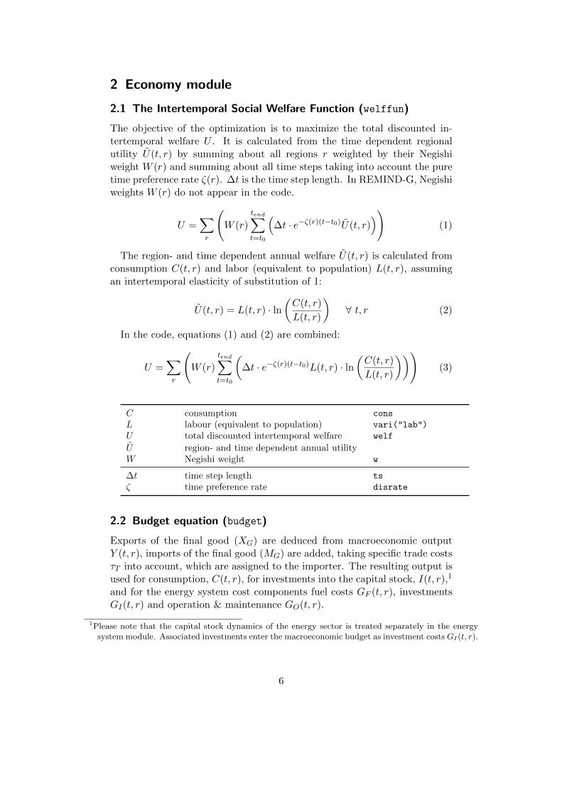
2.1 The Intertemporal Social Welfare Function (welffun)

The objective of the optimization is to maximize the total discounted in-tertemporal welfare U . It is calculated from the time dependent regionalutility U(t, r) by summing about all regions r weighted by their Negishiweight W (r) and summing about all time steps taking into account the puretime preference rate ζ(r). ∆t is the time step length. In REMIND-G, Negishiweights W (r) do not appear in the code.

U =∑r

(W (r)

tend∑t=t0

(∆t · e−ζ(r)(t−t0)U(t, r)

))(1)

The region- and time dependent annual welfare U(t, r) is calculated fromconsumption C(t, r) and labor (equivalent to population) L(t, r), assumingan intertemporal elasticity of substitution of 1:

U(t, r) = L(t, r) · ln(C(t, r)

L(t, r)

)∀ t, r (2)

In the code, equations (1) and (2) are combined:

U =∑r

(W (r)

tend∑t=t0

(∆t · e−ζ(r)(t−t0)L(t, r) · ln

(C(t, r)

L(t, r)

)))(3)

C consumption cons

L labour (equivalent to population) vari("lab")

U total discounted intertemporal welfare welf

U region- and time dependent annual utilityW Negishi weight w

∆t time step length ts

ζ time preference rate disrate

2.2 Budget equation (budget)

Exports of the final good (XG) are deduced from macroeconomic outputY (t, r), imports of the final good (MG) are added, taking specific trade costsτT into account, which are assigned to the importer. The resulting output isused for consumption, C(t, r), for investments into the capital stock, I(t, r),1

and for the energy system cost components fuel costs GF (t, r), investmentsGI(t, r) and operation & maintenance GO(t, r).

1Please note that the capital stock dynamics of the energy sector is treated separately in the energysystem module. Associated investments enter the macroeconomic budget as investment costs GI(t, r).

6

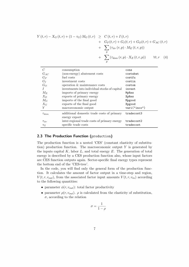
Y (t, r)−XG (t, r) + (1− τG)MG (t, r) ≥ C (t, r) + I (t, r)

+ GF (t, r) +GI(t, r) +GO(t, r) +GAC (t, r)

+∑p

(τitr (r, p) ·ME (t, r, p))

+∑p

(τdom (r, p) ·XE (t, r, p)) ∀t, r (4)

C consumption cons

GAC (non-energy) abatement costs costabat

GF fuel costs costfu

GI investment costs costin

GO operation & maintenance costs costom

I investments into individual stocks of capital invest

ME imports of primary energy MpRes

XE exports of primary energy XpRes

MG imports of the final good Mpgood

XG exports of the final good Xpgood

Y macroeconomic output vari("inco")

τdom additional domestic trade costs of primaryenergy export

tradecost3

τitr inter-regional trade costs of primary energy tradecost2

τG specific trade costs tradecost

2.3 The Production Function (production)

The production function is a nested ’CES’ (constant elasticity of substitu-tion) production function. The macroeconomic output Y is generated bythe inputs capital K, labor L, and total energy E. The generation of totalenergy is described by a CES production function also, whose input factorsare CES function outputs again. Sector-specific final energy types representthe bottom end of the ’CES-tree’.

In the code, you will find only the general form of the production func-tion. It calculates the amount of factor output in a time-step and region,V (t, r, vout), from the associated factor input amounts V (t, r, vin) accordingto the following quantities:

• parameter φ(r, vout): total factor productivity

• parameter ρ(r, vout). ρ is calculated from the elasticity of substitution,σ, according to the relation

σ =1

1− ρ

7

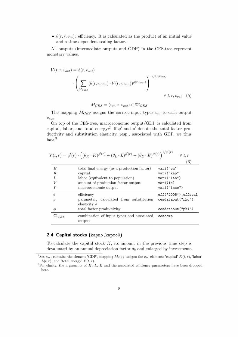
• θ(t, r, vin): efficiency. It is calculated as the product of an initial valueand a time-dependent scaling factor.

All outputs (intermediate outputs and GDP) in the CES-tree representmonetary values.

V (t, r, vout) = φ(r, vout)

·

∑MCES

(θ(t, r, vin) · V (t, r, vin))ρ(r,vout)

1/ρ(r,vout)

∀ t, r, vout (5)

MCES = (vin × vout) ∈MCES

The mapping MCES assigns the correct input types vin to each outputvout.

On top of the CES-tree, macroeconomic output/GDP is calculated fromcapital, labor, and total energy:2 If φ′ and ρ′ denote the total factor pro-ductivity and substitution elasticity, resp., associated with GDP, we thushave3

Y (t, r) = φ′(r) ·(

(θK ·K)ρ′(r) + (θL · L)ρ

′(r) + (θE · E)ρ′(r))1/ρ′(r)

∀ t, r(6)

E total final energy (as a production factor) vari("en"

K capital vari("kap"

L labor (equivalent to population) vari("lab")

V amount of production factor output vari(in)


θ efficiency eff(’2005’),effscal

ρ parameter, calculated from substitutionelasticity σ

cesdataout("rho")

φ total factor productivity cesdataout("phi")

MCES combination of input types and associatedoutput

cescomp

2.4 Capital stocks (kapmo,kapmo0)

To calculate the capital stock K, its amount in the previous time step isdevaluated by an annual depreciation factor δk and enlarged by investments

2Set vout contains the element ’GDP’, mapping MCES assigns the vin-elements ’capital’ K(t, r), ’labor’L(t, r), and ’total energy’ E(t, r).

3For clarity, the arguments of K, L, E and the associated efficiency parameters have been droppedhere.

8

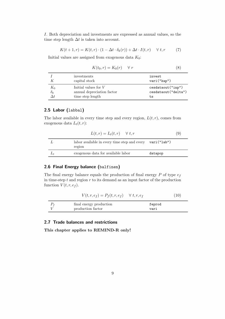
I. Both depreciation and investments are expressed as annual values, so thetime step length ∆t is taken into account.

K(t+ 1, r) = K(t, r) · (1−∆t · δk(r)) + ∆t · I(t, r) ∀ t, r (7)

Initial values are assigned from exogenous data K0:

K(t0, r) = K0(r) ∀ r (8)

I investments invest

K capital stock vari("kap")

K0 Initial values for V cesdataout("inp")

δk annual depreciation factor cesdataout("delta")


2.5 Labor (labbal)

The labor available in every time step and every region, L(t, r), comes fromexogenous data Lt(t, r):

L(t, r) = Lt(t, r) ∀ t, r (9)

L labor available in every time step and everyregion

vari("lab")

Lt exogenous data for available labor datapop

2.6 Final Energy balance (balfinen)

The final energy balance equals the production of final energy P of type efin time-step t and region r to its demand as an input factor of the productionfunction V (t, r, ef ).

V (t, r, ef ) = Pf (t, r, ef ) ∀ t, r, ef (10)

Pf final energy production feprod

V production factor vari

2.7 Trade balances and restrictions

This chapter applies to REMIND-R only!

9

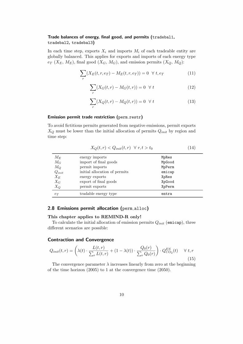
Trade balances of energy, final good, and permits (tradebal1,tradebal2, tradebal3)

In each time step, exports Xi and imports Mi of each tradeable entity areglobally balanced. This applies for exports and imports of each energy typeeT (XE , ME), final good (XG, MG), and emission permits (XQ, MQ):∑

r

(XE(t, r, eT )−ME(t, r, eT )) = 0 ∀ t, eT (11)

∑r

(XG(t, r)−MG(t, r)) = 0 ∀ t (12)

∑r

(XQ(t, r)−MQ(t, r)) = 0 ∀ t (13)

Emission permit trade restriction (perm restr)

To avoid fictitious permits generated from negative emissions, permit exportsXQ must be lower than the initial allocation of permits Qinit by region andtime step:

XQ(t, r) < Qinit(t, r) ∀ r, t > t0 (14)

ME energy imports MpRes

MG import of final goods MpGood

MQ permit imports MpPerm

Qinit initial allocation of permits emicap

XE energy exports XpRes

XG export of final goods XpGood

XQ permit exports XpPerm

eT tradable energy type entra

2.8 Emissions permit allocation (perm alloc)

This chapter applies to REMIND-R only!To calculate the initial allocation of emission permits Qinit (emicap), three

different scenarios are possible:

Contraction and Convergence

Qinit(t, r) =

(λ(t) · L(t, r)∑

r L(t, r)+ (1− λ(t)) · Q0(r)∑

rQ0(r)

)·QESCO2

(t) ∀ t, r

(15)The convergence parameter λ increases linearly from zero at the beginning

of the time horizon (2005) to 1 at the convergence time (2050).

10

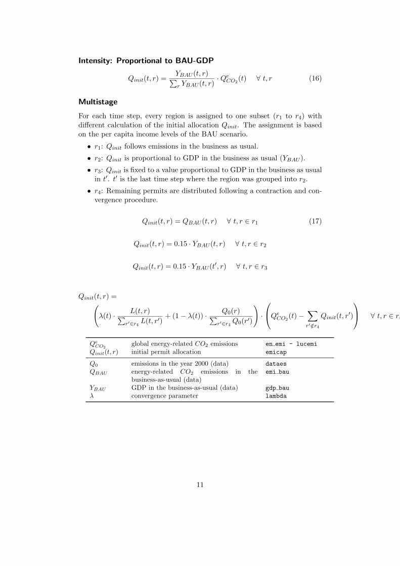
Intensity: Proportional to BAU-GDP

Qinit(t, r) =YBAU (t, r)∑r YBAU (t, r)

·QeCO2(t) ∀ t, r (16)

Multistage

For each time step, every region is assigned to one subset (r1 to r4) withdifferent calculation of the initial allocation Qinit. The assignment is basedon the per capita income levels of the BAU scenario.

• r1: Qinit follows emissions in the business as usual.

• r2: Qinit is proportional to GDP in the business as usual (YBAU ).

• r3: Qinit is fixed to a value proportional to GDP in the business as usualin t′. t′ is the last time step where the region was grouped into r2.

• r4: Remaining permits are distributed following a contraction and con-vergence procedure.

Qinit(t, r) = QBAU (t, r) ∀ t, r ∈ r1 (17)

Qinit(t, r) = 0.15 · YBAU (t, r) ∀ t, r ∈ r2

Qinit(t, r) = 0.15 · YBAU (t′, r) ∀ t, r ∈ r3

Qinit(t, r) =(λ(t) · L(t, r)∑

r′∈r4 L(t, r′)+ (1− λ(t)) · Q0(r)∑

r′∈r4 Q0(r′)

)·

QeCO2(t)−

∑r′ /∈r4

Qinit(t, r′)

∀ t, r ∈ r4

QeCO2global energy-related CO2 emissions en emi - lucemi

Qinit(t, r) initial permit allocation emicap

Q0 emissions in the year 2000 (data) dataes

QBAU energy-related CO2 emissions in thebusiness-as-usual (data)

emi bau

YBAU GDP in the business-as-usual (data) gdp bau

λ convergence parameter lambda

11

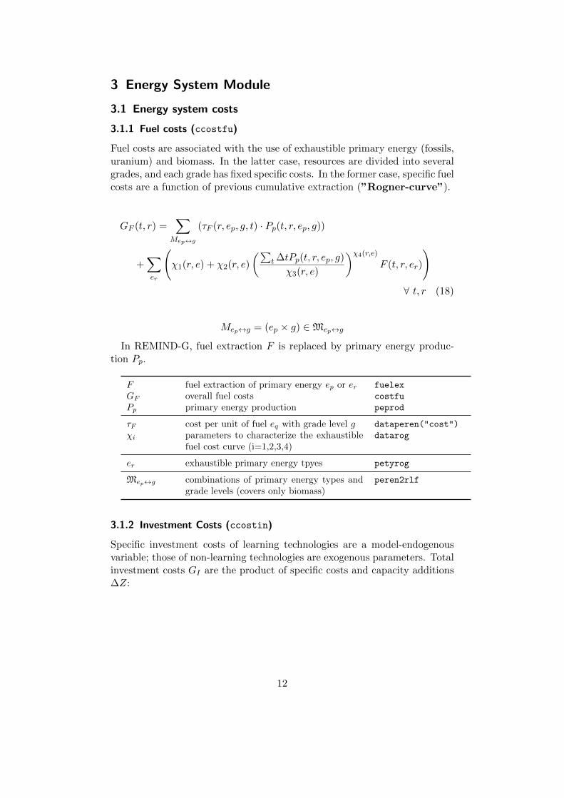
3 Energy System Module

3.1 Energy system costs

3.1.1 Fuel costs (ccostfu)

Fuel costs are associated with the use of exhaustible primary energy (fossils,uranium) and biomass. In the latter case, resources are divided into severalgrades, and each grade has fixed specific costs. In the former case, specific fuelcosts are a function of previous cumulative extraction (”Rogner-curve”).

GF (t, r) =∑

Mep↔g

(τF (r, ep, g, t) · Pp(t, r, ep, g))

+∑er

(χ1(r, e) + χ2(r, e)

(∑t ∆tPp(t, r, ep, g)

χ3(r, e)

)χ4(r,e)

F (t, r, er)

)∀ t, r (18)

Mep↔g = (ep × g) ∈Mep↔g

In REMIND-G, fuel extraction F is replaced by primary energy produc-tion Pp.

F fuel extraction of primary energy ep or er fuelex

GF overall fuel costs costfu

Pp primary energy production peprod

τF cost per unit of fuel eq with grade level g dataperen("cost")

χi parameters to characterize the exhaustiblefuel cost curve (i=1,2,3,4)

datarog

er exhaustible primary energy tpyes petyrog

Mep↔g combinations of primary energy types andgrade levels (covers only biomass)

peren2rlf

3.1.2 Investment Costs (ccostin)

Specific investment costs of learning technologies are a model-endogenousvariable; those of non-learning technologies are exogenous parameters. Totalinvestment costs GI are the product of specific costs and capacity additions∆Z:

12

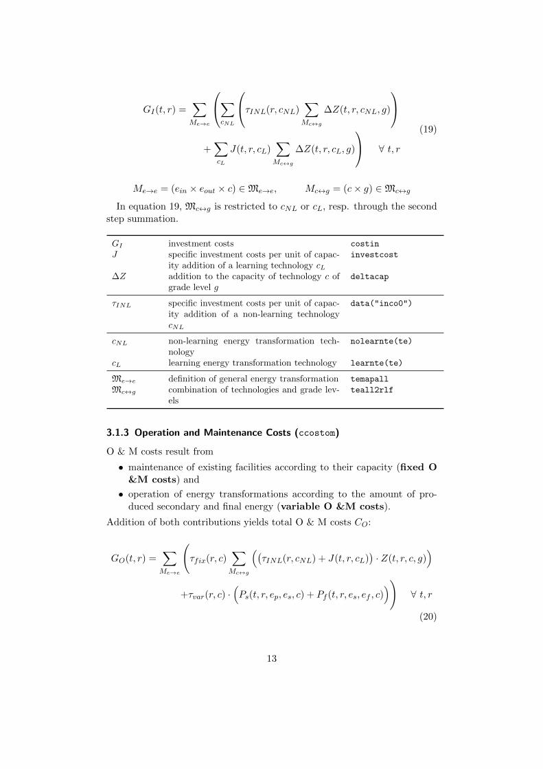
GI(t, r) =∑Me→e

∑cNL

τINL(r, cNL)∑Mc↔g

∆Z(t, r, cNL, g)

+∑cL

J(t, r, cL)∑Mc↔g

∆Z(t, r, cL, g)

∀ t, r

(19)

Me→e = (ein × eout × c) ∈Me→e, Mc↔g = (c× g) ∈Mc↔g

In equation 19, Mc↔g is restricted to cNL or cL, resp. through the secondstep summation.

GI investment costs costin

J specific investment costs per unit of capac-ity addition of a learning technology cL

investcost

∆Z addition to the capacity of technology c ofgrade level g

deltacap

τINL specific investment costs per unit of capac-ity addition of a non-learning technologycNL

data("inco0")

cNL non-learning energy transformation tech-nology

nolearnte(te)

cL learning energy transformation technology learnte(te)

Me→e definition of general energy transformation temapall

Mc↔g combination of technologies and grade lev-els

teall2rlf

3.1.3 Operation and Maintenance Costs (ccostom)

O & M costs result from

• maintenance of existing facilities according to their capacity (fixed O&M costs) and

• operation of energy transformations according to the amount of pro-duced secondary and final energy (variable O &M costs).

Addition of both contributions yields total O & M costs CO:

GO(t, r) =∑Me→e

(τfix(r, c)

∑Mc↔g

((τINL(r, cNL) + J(t, r, cL)

)· Z(t, r, c, g)

)

+τvar(r, c) ·(Ps(t, r, ep, es, c) + Pf (t, r, es, ef , c)

))∀ t, r

(20)

13

Me→e = (ein × eout × c) ∈Me→e, Mc↔g = (c× g) ∈Mc↔g


J specific investment costs for adding capac-ity of a learning technology cL

investcost

Ps production of secondary energy seprod

Pf production of final energy feprod

Z capacity of technology c cap



τfix fixed specific O&M costs data("omf")


data("inco0")

τvar variable specific O&M costs data("omv")


nolearnte(te)




teall2rlf

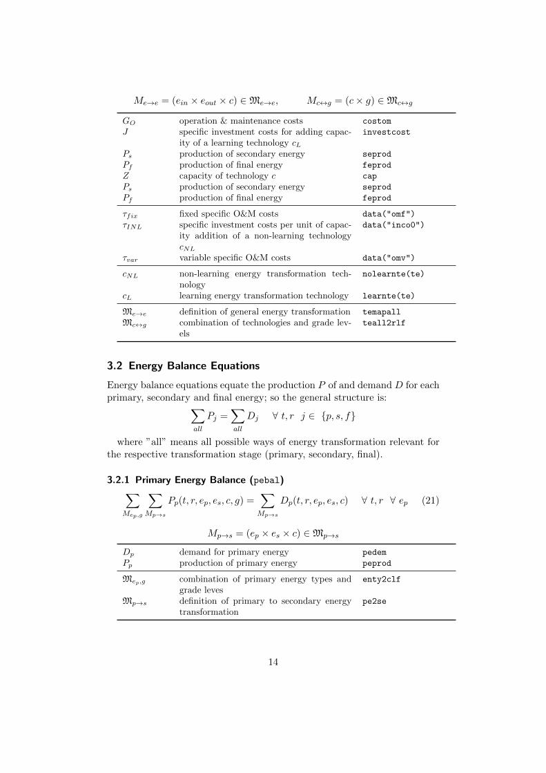
3.2 Energy Balance Equations

Energy balance equations equate the production P of and demand D for eachprimary, secondary and final energy; so the general structure is:∑

all

Pj =∑all

Dj ∀ t, r j ∈ {p, s, f}

where ”all” means all possible ways of energy transformation relevant forthe respective transformation stage (primary, secondary, final).

3.2.1 Primary Energy Balance (pebal)∑Mep,g

∑Mp→s

Pp(t, r, ep, es, c, g) =∑Mp→s

Dp(t, r, ep, es, c) ∀ t, r ∀ ep (21)

Mp→s = (ep × es × c) ∈Mp→s

Dp demand for primary energy pedem

Pp production of primary energy peprod

Mep,g combination of primary energy types andgrade leves

enty2clf

Mp→s definition of primary to secondary energytransformation

pe2se

14

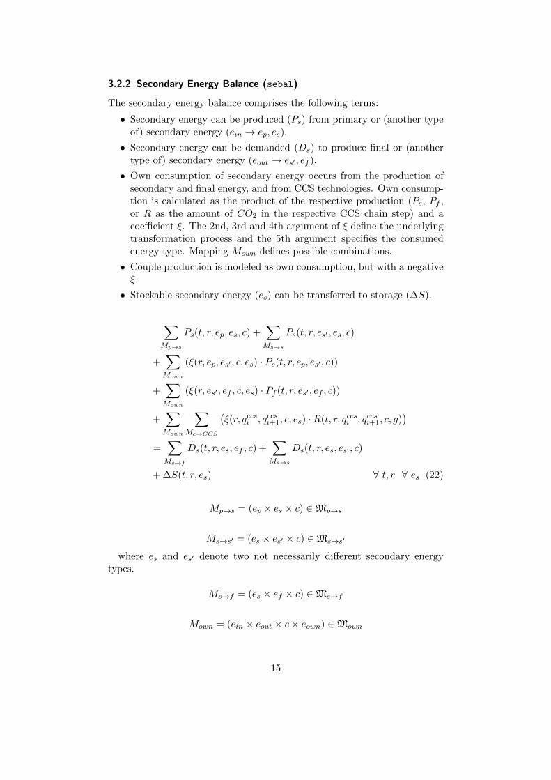
3.2.2 Secondary Energy Balance (sebal)

The secondary energy balance comprises the following terms:

• Secondary energy can be produced (Ps) from primary or (another typeof) secondary energy (ein → ep, es).

• Secondary energy can be demanded (Ds) to produce final or (anothertype of) secondary energy (eout → es′ , ef ).

• Own consumption of secondary energy occurs from the production ofsecondary and final energy, and from CCS technologies. Own consump-tion is calculated as the product of the respective production (Ps, Pf ,or R as the amount of CO2 in the respective CCS chain step) and acoefficient ξ. The 2nd, 3rd and 4th argument of ξ define the underlyingtransformation process and the 5th argument specifies the consumedenergy type. Mapping Mown defines possible combinations.

• Couple production is modeled as own consumption, but with a negativeξ.

• Stockable secondary energy (es) can be transferred to storage (∆S).

∑Mp→s

Ps(t, r, ep, es, c) +∑Ms→s

Ps(t, r, es′ , es, c)

+∑Mown

(ξ(r, ep, es′ , c, es) · Ps(t, r, ep, es′ , c))

+∑Mown

(ξ(r, es′ , ef , c, es) · Pf (t, r, es′ , ef , c))

+∑Mown

∑Mc→CCS

(ξ(r, qccsi , qccsi+1, c, es) ·R(t, r, qccsi , qccsi+1, c, g)

)=∑Ms→f

Ds(t, r, es, ef , c) +∑Ms→s

Ds(t, r, es, es′ , c)

+ ∆S(t, r, es) ∀ t, r ∀ es (22)


Ms→s′ = (es × es′ × c) ∈Ms→s′

where es and es′ denote two not necessarily different secondary energytypes.

Ms→f = (es × ef × c) ∈Ms→f

Mown = (ein × eout × c× eown) ∈Mown

15

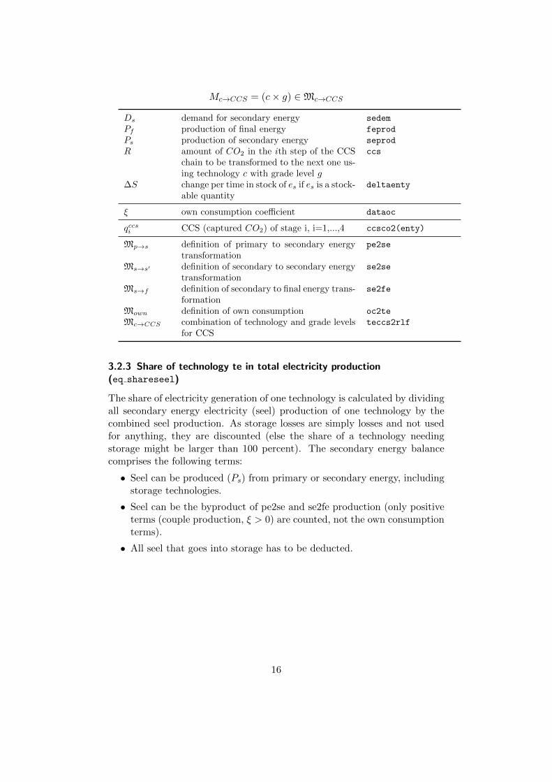
Mc→CCS = (c× g) ∈Mc→CCS

Ds demand for secondary energy sedem



R amount of CO2 in the ith step of the CCSchain to be transformed to the next one us-ing technology c with grade level g

ccs

∆S change per time in stock of es if es is a stock-able quantity

deltaenty

ξ own consumption coefficient dataoc

qccsi CCS (captured CO2) of stage i, i=1,...,4 ccsco2(enty)


pe2se

Ms→s′ definition of secondary to secondary energytransformation

se2se

Ms→f definition of secondary to final energy trans-formation

se2fe

Mown definition of own consumption oc2te

Mc→CCS combination of technology and grade levelsfor CCS

teccs2rlf

3.2.3 Share of technology te in total electricity production(eq shareseel)

The share of electricity generation of one technology is calculated by dividingall secondary energy electricity (seel) production of one technology by thecombined seel production. As storage losses are simply losses and not usedfor anything, they are discounted (else the share of a technology needingstorage might be larger than 100 percent). The secondary energy balancecomprises the following terms:

• Seel can be produced (Ps) from primary or secondary energy, includingstorage technologies.

• Seel can be the byproduct of pe2se and se2fe production (only positiveterms (couple production, ξ > 0) are counted, not the own consumptionterms).

• All seel that goes into storage has to be deducted.

16

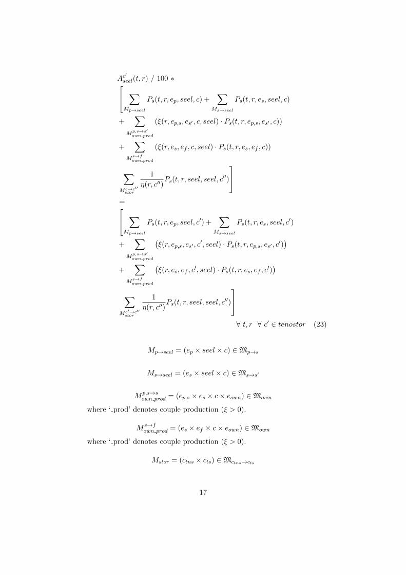
Ac′seel(t, r) / 100 ∗ ∑Mp→seel

Ps(t, r, ep, seel, c) +∑

Ms→seel

Ps(t, r, es, seel, c)

+∑

Mp,s→s′own prod

(ξ(r, ep,s, es′ , c, seel) · Ps(t, r, ep,s, es′ , c))

+∑

Ms→fown prod

(ξ(r, es, ef , c, seel) · Ps(t, r, es, ef , c))

∑Mc→c′′

stor

1

η(r, c′′)Ps(t, r, seel, seel, c

′′)

= ∑Mp→seel

Ps(t, r, ep, seel, c′) +

∑Ms→seel

Ps(t, r, es, seel, c′)

+∑

Mp,s→s′own prod

(ξ(r, ep,s, es′ , c

′, seel) · Ps(t, r, ep,s, es′ , c′))

+∑

Ms→fown prod

(ξ(r, es, ef , c

′, seel) · Ps(t, r, es, ef , c′))

∑Mc′→c′′

stor

1

η(r, c′′)Ps(t, r, seel, seel, c

′′)

∀ t, r ∀ c′ ∈ tenostor (23)

Mp→seel = (ep × seel × c) ∈Mp→s

Ms→seel = (es × seel × c) ∈Ms→s′

Mp,s→sown prod = (ep,s × es × c× eown) ∈Mown

where ‘ prod’ denotes couple production (ξ > 0).

M s→fown prod = (es × ef × c× eown) ∈Mown

where ‘ prod’ denotes couple production (ξ > 0).

Mstor = (ctns × cts) ∈Mctns→cts

17

Ac′

seel share of electricity generation by technologyc’

v shareseel




η efficiency of technology c, can depend ontime or not

data("eta"),

dataeta

ctns technologies that require storage teneedstor

cts technologies that store electricity testor


pe2se


se2se


se2fe


Mctns→cts definition of storage requirements te2stor

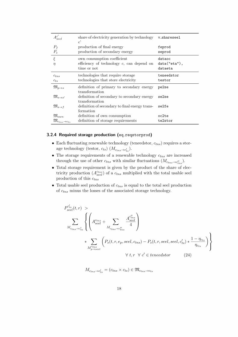
3.2.4 Required storage production (eq reqstorprod)

• Each fluctuating renewable technology (teneedstor, ctns) requires a stor-age technology (testor, cts) (Mctns→c′ts).

• The storage requirements of a renewable technology ctns are increasedthrough the use of other ctns with similar fluctuations (Mctns→c′′tns

).

• Total storage requirement is given by the product of the share of elec-tricity production (Actns

seel ) of a ctns multiplied with the total usable seelproduction of this ctns

• Total usable seel production of ctns is equal to the total seel productionof ctns minus the losses of the associated storage technology.

Pc′tsseel(t, r) >

∑Mctns→c′ts

Actns

seel +∑

Mctns→c′′tns

Ac′′tnsseel

4

∗∑

Mctnsp→seel

(Ps(t, r, ep, seel, ctns)− Ps(t, r, seel, seel, c′ts) ∗

1− ηctsηcts

)∀ t, r ∀ c′ ∈ teneedstor (24)

Mctns→c′ts = (ctns × cts) ∈Mctns→cts

18

Mctns→c′′tns= (ctns × c′′tns) ∈Mctns→ctns

M ctnsp→seel = (ep × seel × ctns) ∈Mp→s

Acseel share of electricity generation by technologyc

v shareseel

Ps production of secondary energy s seprod

ηc efficiency of technology c, can depend ontime or not

data("eta"),

dataeta




Mctns→ctnsdefinition of similar fluctuation patterns te2teneedstorlinked


pe2se

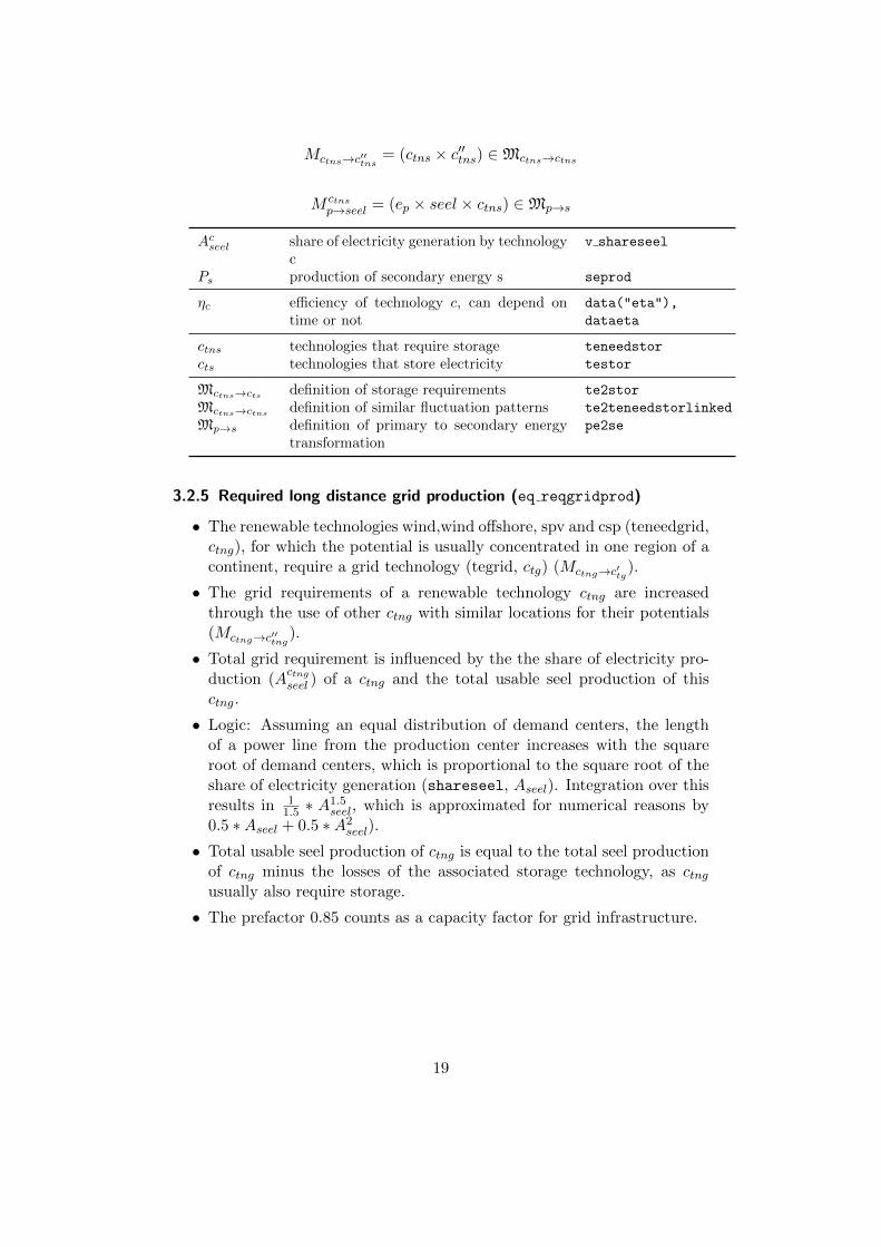
3.2.5 Required long distance grid production (eq reqgridprod)

• The renewable technologies wind,wind offshore, spv and csp (teneedgrid,ctng), for which the potential is usually concentrated in one region of acontinent, require a grid technology (tegrid, ctg) (Mctng→c′tg).

• The grid requirements of a renewable technology ctng are increasedthrough the use of other ctng with similar locations for their potentials(Mctng→c′′tng

).

• Total grid requirement is influenced by the the share of electricity pro-duction (A

ctng

seel ) of a ctng and the total usable seel production of thisctng.

• Logic: Assuming an equal distribution of demand centers, the lengthof a power line from the production center increases with the squareroot of demand centers, which is proportional to the square root of theshare of electricity generation (shareseel, Aseel). Integration over thisresults in 1

1.5 ∗ A1.5seel, which is approximated for numerical reasons by

0.5 ∗Aseel + 0.5 ∗A2seel).

• Total usable seel production of ctng is equal to the total seel productionof ctng minus the losses of the associated storage technology, as ctngusually also require storage.

• The prefactor 0.85 counts as a capacity factor for grid infrastructure.

19

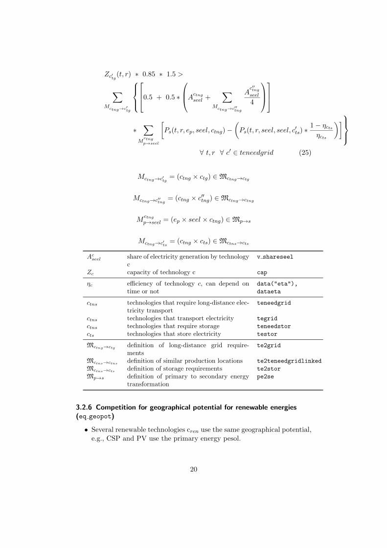
Zc′tg(t, r) ∗ 0.85 ∗ 1.5 >

∑Mctng→c′tg

0.5 + 0.5 ∗

Actng

seel +∑

Mctng→c′′tng

Ac′′tng

seel

4

∗∑

Mctngp→seel

[Ps(t, r, ep, seel, ctng)−

(Ps(t, r, seel, seel, c

′ts) ∗

1− ηctsηcts

)]∀ t, r ∀ c′ ∈ teneedgrid (25)

Mctng→c′tg = (ctng × ctg) ∈Mctng→ctg

Mctng→c′′tng= (ctng × c′′tng) ∈Mctng→ctng

Mctng

p→seel = (ep × seel × ctng) ∈Mp→s

Mctng→c′ts = (ctng × cts) ∈Mctns→cts

Acseel share of electricity generation by technologyc

v shareseel

Zc capacity of technology c cap

ηc efficiency of technology c, can depend ontime or not

data("eta"),

dataeta

ctns technologies that require long-distance elec-tricity transport

teneedgrid

ctns technologies that transport electricity tegrid



Mctng→ctg definition of long-distance grid require-ments

te2grid

Mctns→ctnsdefinition of similar production locations te2teneedgridlinked



pe2se

3.2.6 Competition for geographical potential for renewable energies(eq geopot)

• Several renewable technologies cren use the same geographical potential,e.g., CSP and PV use the primary energy pesol.

20

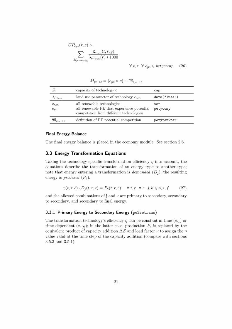
GPepc(r, g) >∑Mpc→cren

Zcren(t, r, g)

λµcren(r) ∗ 1000

∀ t, r ∀ epc ∈ petycomp (26)

Mpc→c = (epc × c) ∈Mepc→c

Zc capacity of technology c cap

λµcren land use parameter of technology cren data("luse")

cren all renewable technologies ter

epc all renewable PE that experience potentialcompetition from different technologies

petycomp

Mepc→c definition of PE potential competition petyren2ter

Final Energy Balance

The final energy balance is placed in the economy module. See section 2.6.

3.3 Energy Transformation Equations

Taking the technology-specific transformation efficiency η into account, theequations describe the transformation of an energy type to another type;note that energy entering a transformation is demanded (Dj), the resultingenergy is produced (Pk):

η(t, r, c) ·Dj(t, r, c) = Pk(t, r, c) ∀ t, r ∀ c j, k ∈ p, s, f (27)

and the allowed combinations of j and k are primary to secondary, secondaryto secondary, and secondary to final energy.

3.3.1 Primary Energy to Secondary Energy (pe2setrans)

The transformation technology’s efficiency η can be constant in time (cηc) ortime dependent (cη(t)); in the latter case, production Ps is replaced by theequivalent product of capacity addition ∆Z and load factor ν to assign the ηvalue valid at the time step of the capacity addition (compare with sections3.5.3 and 3.5.1):

21

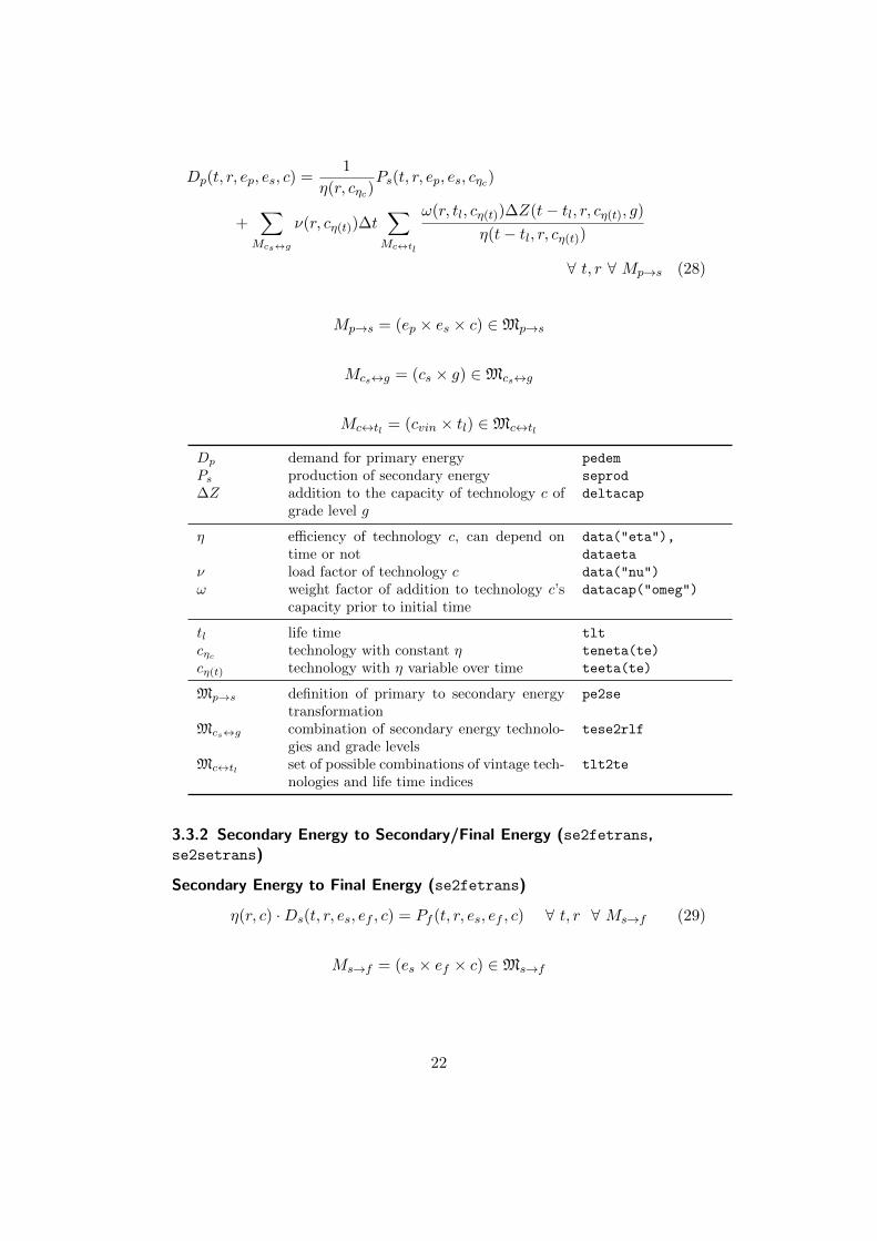
Dp(t, r, ep, es, c) =1

η(r, cηc)Ps(t, r, ep, es, cηc)

+∑

Mcs↔g

ν(r, cη(t))∆t∑Mc↔tl

ω(r, tl, cη(t))∆Z(t− tl, r, cη(t), g)

η(t− tl, r, cη(t))

∀ t, r ∀ Mp→s (28)


Mcs↔g = (cs × g) ∈Mcs↔g

Mc↔tl = (cvin × tl) ∈Mc↔tl

Dp demand for primary energy pedem



deltacap


data("eta"),

dataeta

ν load factor of technology c data("nu")

ω weight factor of addition to technology c’scapacity prior to initial time

datacap("omeg")

tl life time tlt

cηc technology with constant η teneta(te)

cη(t) technology with η variable over time teeta(te)


pe2se

Mcs↔g combination of secondary energy technolo-gies and grade levels

tese2rlf

Mc↔tl set of possible combinations of vintage tech-nologies and life time indices

tlt2te

3.3.2 Secondary Energy to Secondary/Final Energy (se2fetrans,se2setrans)

Secondary Energy to Final Energy (se2fetrans)

η(r, c) ·Ds(t, r, es, ef , c) = Pf (t, r, es, ef , c) ∀ t, r ∀ Ms→f (29)

Ms→f = (es × ef × c) ∈Ms→f

22

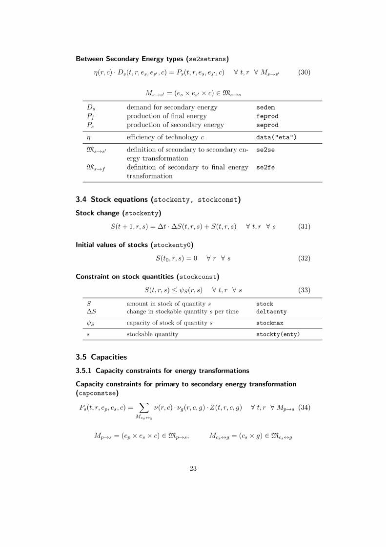
Between Secondary Energy types (se2setrans)

η(r, c) ·Ds(t, r, es, es′ , c) = Ps(t, r, es, es′ , c) ∀ t, r ∀ Ms→s′ (30)

Ms→s′ = (es × es′ × c) ∈Ms→s

Ds demand for secondary energy sedem



η efficiency of technology c data("eta")

Ms→s′ definition of secondary to secondary en-ergy transformation

se2se

Ms→f definition of secondary to final energytransformation

se2fe

3.4 Stock equations (stockenty, stockconst)

Stock change (stockenty)

S(t+ 1, r, s) = ∆t ·∆S(t, r, s) + S(t, r, s) ∀ t, r ∀ s (31)

Initial values of stocks (stockenty0)

S(t0, r, s) = 0 ∀ r ∀ s (32)

Constraint on stock quantities (stockconst)

S(t, r, s) ≤ ψS(r, s) ∀ t, r ∀ s (33)

S amount in stock of quantity s stock

∆S change in stockable quantity s per time deltaenty

ψS capacity of stock of quantity s stockmax

s stockable quantity stockty(enty)

3.5 Capacities

3.5.1 Capacity constraints for energy transformations

Capacity constraints for primary to secondary energy transformation(capconstse)

Ps(t, r, ep, es, c) =∑

Mcs↔g

ν(r, c) · νg(r, c, g) ·Z(t, r, c, g) ∀ t, r ∀ Mp→s (34)

Mp→s = (ep × es × c) ∈Mp→s, Mcs↔g = (cs × g) ∈Mcs↔g

23

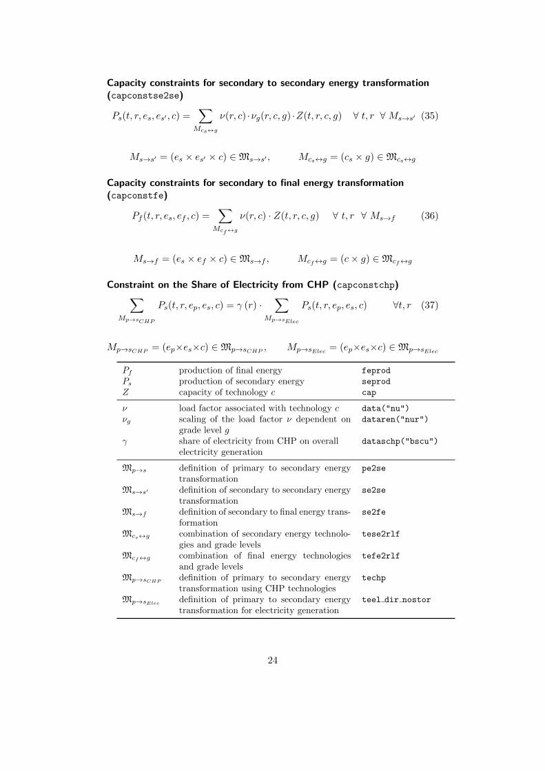
Capacity constraints for secondary to secondary energy transformation(capconstse2se)

Ps(t, r, es, es′ , c) =∑

Mcs↔g

ν(r, c) ·νg(r, c, g) ·Z(t, r, c, g) ∀ t, r ∀Ms→s′ (35)

Ms→s′ = (es × es′ × c) ∈Ms→s′ , Mcs↔g = (cs × g) ∈Mcs↔g

Capacity constraints for secondary to final energy transformation(capconstfe)

Pf (t, r, es, ef , c) =∑

Mcf↔g

ν(r, c) · Z(t, r, c, g) ∀ t, r ∀ Ms→f (36)

Ms→f = (es × ef × c) ∈Ms→f , Mcf↔g = (c× g) ∈Mcf↔g

Constraint on the Share of Electricity from CHP (capconstchp)∑Mp→sCHP

Ps(t, r, ep, es, c) = γ (r) ·∑

Mp→sElec

Ps(t, r, ep, es, c) ∀t, r (37)

Mp→sCHP = (ep×es×c) ∈Mp→sCHP , Mp→sElec= (ep×es×c) ∈Mp→sElec




ν load factor associated with technology c data("nu")

νg scaling of the load factor ν dependent ongrade level g

dataren("nur")

γ share of electricity from CHP on overall dataschp("bscu")

electricity generation


pe2se


se2se


se2fe


tese2rlf

Mcf↔g combination of final energy technologiesand grade levels

tefe2rlf

Mp→sCHPdefinition of primary to secondary energytransformation using CHP technologies

techp

Mp→sElecdefinition of primary to secondary energytransformation for electricity generation

teel dir nostor

24

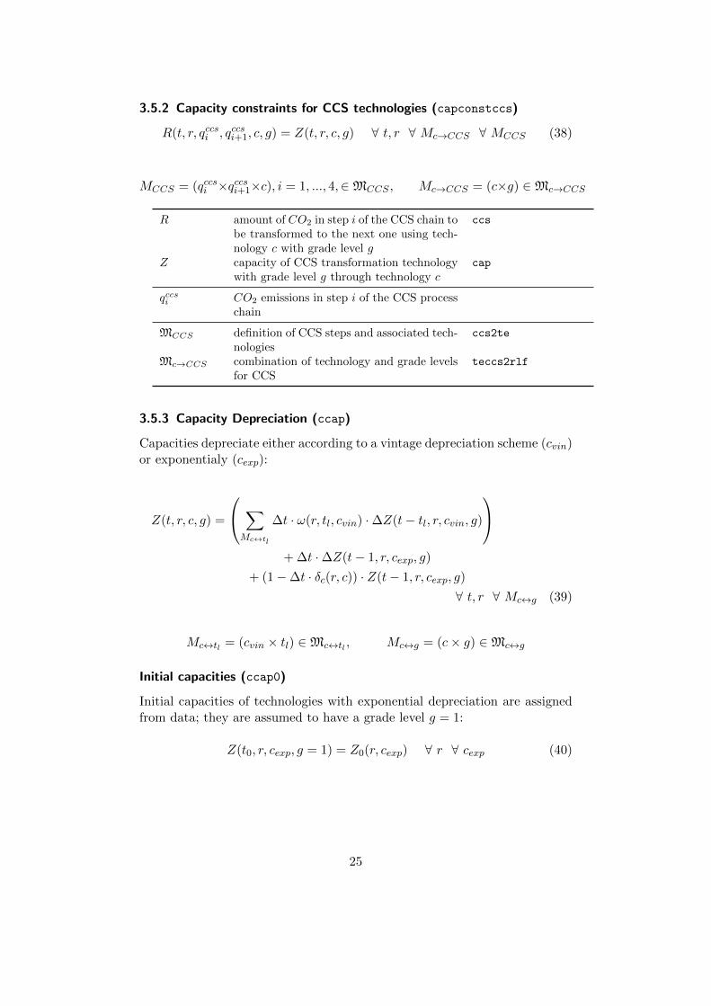
3.5.2 Capacity constraints for CCS technologies (capconstccs)

R(t, r, qccsi , qccsi+1, c, g) = Z(t, r, c, g) ∀ t, r ∀ Mc→CCS ∀ MCCS (38)

MCCS = (qccsi ×qccsi+1×c), i = 1, ..., 4,∈MCCS , Mc→CCS = (c×g) ∈Mc→CCS

R amount of CO2 in step i of the CCS chain tobe transformed to the next one using tech-nology c with grade level g

ccs

Z capacity of CCS transformation technologywith grade level g through technology c

cap

qccsi CO2 emissions in step i of the CCS processchain

MCCS definition of CCS steps and associated tech-nologies

ccs2te


teccs2rlf

3.5.3 Capacity Depreciation (ccap)

Capacities depreciate either according to a vintage depreciation scheme (cvin)or exponentialy (cexp):

Z(t, r, c, g) =

∑Mc↔tl

∆t · ω(r, tl, cvin) ·∆Z(t− tl, r, cvin, g)

+ ∆t ·∆Z(t− 1, r, cexp, g)

+ (1−∆t · δc(r, c)) · Z(t− 1, r, cexp, g)

∀ t, r ∀ Mc↔g (39)

Mc↔tl = (cvin × tl) ∈Mc↔tl , Mc↔g = (c× g) ∈Mc↔g

Initial capacities (ccap0)

Initial capacities of technologies with exponential depreciation are assignedfrom data; they are assumed to have a grade level g = 1:

Z(t0, r, cexp, g = 1) = Z0(r, cexp) ∀ r ∀ cexp (40)

25


∆Z addition of capacity deltacap

δc depreciation of technology c data("delta")


datacap("omeg")

Z0 initial capacity of technology cexp data("cap0")

tl life time tlt

cexp technologies with exponential capacity de-preciation

expte(te)

cvin technologies with vintage capacity depreci-ation

vinte(te)


teall2rlf


tlt2te

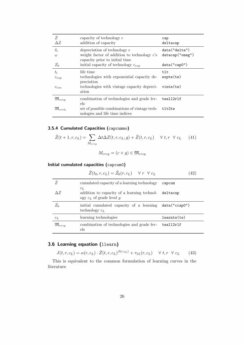
3.5.4 Cumulated Capacities (capcummo)

Z(t+ 1, r, cL) =∑Mc↔g

∆t∆Z(t, r, cL, g) + Z(t, r, cL) ∀ t, r ∀ cL (41)

Mc↔g = (c× g) ∈Mc↔g

Initial cumulated capacities (capcum0)

Z(t0, r, cL) = Z0(r, cL) ∀ r ∀ cL (42)

Z cumulated capacity of a learning technologycL

capcum

∆Z addition to capacity of a learning technol-ogy cL of grade level g

deltacap

Z0 initial cumulated capacity of a learningtechnology cL

data("ccap0")

cL learning technologies learnte(te)


teall2rlf

3.6 Learning equation (llearn)

J(t, r, cL) = α(r, cL) · Z(t, r, cL)β(r,cL) + τIL(r, cL) ∀ t, r ∀ cL (43)

This is equivalent to the common formulation of learning curves in theliterature

26

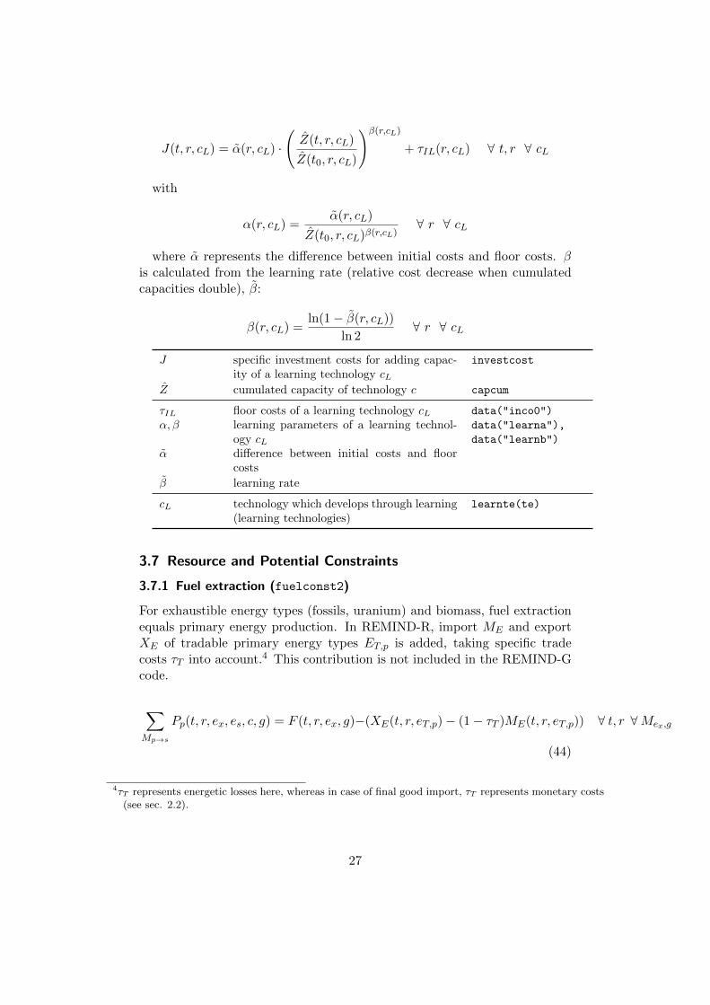
J(t, r, cL) = α(r, cL) ·

(Z(t, r, cL)

Z(t0, r, cL)

)β(r,cL)+ τIL(r, cL) ∀ t, r ∀ cL

with

α(r, cL) =α(r, cL)

Z(t0, r, cL)β(r,cL)∀ r ∀ cL

where α represents the difference between initial costs and floor costs. βis calculated from the learning rate (relative cost decrease when cumulatedcapacities double), β:

β(r, cL) =ln(1− β(r, cL))

ln 2∀ r ∀ cL

J specific investment costs for adding capac-ity of a learning technology cL

investcost

Z cumulated capacity of technology c capcum

τIL floor costs of a learning technology cL data("inco0")

α, β learning parameters of a learning technol-ogy cL

data("learna"),

data("learnb")

α difference between initial costs and floorcosts

β learning rate

cL technology which develops through learning(learning technologies)

learnte(te)

3.7 Resource and Potential Constraints

3.7.1 Fuel extraction (fuelconst2)

For exhaustible energy types (fossils, uranium) and biomass, fuel extractionequals primary energy production. In REMIND-R, import ME and exportXE of tradable primary energy types ET,p is added, taking specific tradecosts τT into account.4 This contribution is not included in the REMIND-Gcode.

∑Mp→s

Pp(t, r, ex, es, c, g) = F (t, r, ex, g)−(XE(t, r, eT,p)− (1− τT )ME(t, r, eT,p)) ∀ t, r ∀Mex,g

(44)

4τT represents energetic losses here, whereas in case of final good import, τT represents monetary costs(see sec. 2.2).

27

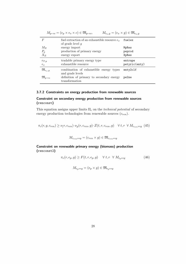
Mp→s = (ep × es × c) ∈Mp→s, Mex,g = (ex × g) ∈Mex,g

F fuel extraction of an exhaustible resource exof grade level g

fuelex

ME energy import MpRes


XE energy export XpRes

eT,p tradable primary energy type entrape

ex exhaustible resource petyric(enty)

Mex,g combination of exhaustible energy typesand grade levels

enty2clf


pe2se

3.7.2 Constraints on energy production from renewable sources

Constraint on secondary energy production from renewable sources(renconst)

This equation assigns upper limits Πc on the technical potential of secondaryenergy production technologies from renewable sources (cren).

πc(r, g, cren) ≥ ν(r, cren)·νg(r, cren, g)·Z(t, r, cren, g) ∀ t, r ∀Mcren↔g (45)

Mcren↔g = (cren × g) ∈Mcren↔g

Constraint on renewable primary energy (biomass) production(renconst2)

πe(r, ep, g) ≥ F (t, r, ep, g) ∀ t, r ∀ Mep↔g (46)

Mep↔g = (ep × g) ∈Mep↔g

28

F extraction of primary resource ep of gradelevel g

fuelex




dataren("nur")

πc maximal production (according to technol-ogy cren) of secondary energy from non-exhaustible resource via cren, g

dataren("maxprod")

πe maximal production of primary energy fromprimary resource ep of grade level g

dataperen("maxprod")

cren renewable energy transformation technolo-gies

ter(te)

Mcren↔g combination of renewable technologies andgrade levels (mapping Mc↔g is restricted onsubset cren)

teall2rlf

Mep↔g combinations of primary renewable energytypes and grade levels

peren2rlf

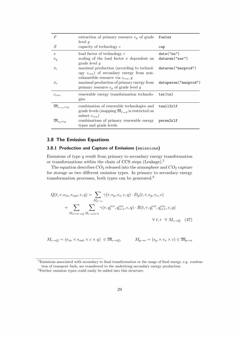
3.8 The Emission Equations

3.8.1 Production and Capture of Emissions (emissions)

Emissions of type q result from primary to secondary energy transformationor transformations within the chain of CCS steps (Leakage).5

The equation describes CO2 released into the atmosphere and CO2 capturefor storage as two different emission types. In primary to secondary energytransformation processes, both types can be generated.6

Q(t, r, ein, eout, c, q) =∑Mp→s

γ(r, ep, es, c, q) ·Dp(t, r, ep, es, c)

+∑

MCCS→Q

∑Mc→CCS

γ(r, qccsi , qccsi+1, c, q) ·R(t, r, qccsi , qccsi+1, c, g)

∀ t, r ∀ Mc→Q (47)

Mc→Q = (ein × eout × c× q) ∈Mc→Q, Mp→s = (ep × es × c) ∈Mp→s

5Emissions associated with secondary to final transformation or the usage of final energy, e.g. combus-tion of transport fuels, are transferred to the underlying secondary energy production.

6Further emission types could easily be added into this structure.

29

Dp demand of primary energy pedem


Q amount of emissions from type q producedby conversions explained in Mc→Q

emi

R transformation in the CCS chain from stepqccsi to qccsi+1 using technology c with gradelevel g

ccs

γ emission of type q per energy flow in thetransformation ein into eout using c

dataemi

q emission type (CO2, captured CO2) enty


MCCS→Q definition of leakage from CCS transforma-tions

ccs2tele


teccs2rlf

Mc→Q definition of emissions from a transforma-tion

emi2te


pe2se

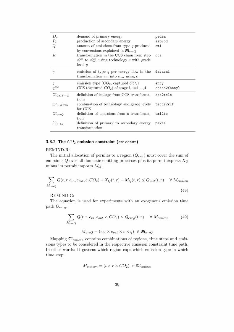
3.8.2 The CO2 emission constraint (emiconst)

REMIND-R:The initial allocation of permits to a region (Qinit) must cover the sum of

emissions Q over all domestic emitting processes plus its permit exports XQ

minus its permit imports MQ.

∑Mc→Q

Q(t, r, ein, eout, c, CO2) +XQ(t, r)−MQ(t, r) ≤ Qinit(t, r) ∀ Memicon

(48)REMIND-G:The equation is used for experiments with an exogenous emission time

path Qexog.∑Mc→Q

Q(t, r, ein, eout, c, CO2) ≤ Qexog(t, r) ∀ Memicon (49)

Mc→Q = (ein × eout × c× q) ∈Mc→Q

Mapping Memicon contains combinations of regions, time steps and emis-sions types to be considered in the respective emission constraint time path.In other words: It governs which region caps which emission type in whichtime step:

Memicon = (t× r × CO2) ∈Memicon

30

ME emissions permit import MpPerm

Q amount of emissions from type q = CO2

produced by conversions specified in Mc→Q

emi

Qinit initial permit allocation emicap

XE emissions permit export XpPerm

Qexog exogenous time path for energy-related to-tal CO2 emissions

dataemiconst


emi2te

Memicon combination of regions, time steps andemission types to be considered in the re-spective emission constraint

emicon

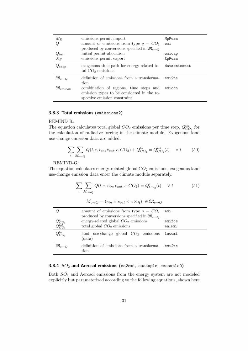
3.8.3 Total emissions (emissions2)

REMIND-R:The equation calculates total global CO2 emissions per time step, QtotCO2

forthe calculation of radiative forcing in the climate module. Exogenous landuse-change emission data are added.∑

r

∑Mc→Q

Q(t, r, ein, eout, c, CO2) +QluCO2= QtotCO2

(t) ∀ t (50)

REMIND-G:The equation calculates energy-related global CO2 emissions, exogenous landuse-change emission data enter the climate module separately.∑

r

∑Mc→Q

Q(t, r, ein, eout, c, CO2) = QeCO2(t) ∀ t (51)

Mc→Q = (ein × eout × c× q) ∈Mc→Q

Q amount of emissions from type q = CO2

produced by conversions specified in Mc→Q

emi

QeCO2energy-related global CO2 emissions emifos

QtotCO2total global CO2 emissions en emi

QluCO2land use-change global CO2 emissions(data)

lucemi


emi2te

3.8.4 SO2 and Aerosol emissions (so2emi, cscouple, cscouple0)

Both SO2 and Aerosol emissions from the energy system are not modeledexplicitly but parameterized according to the following equations, shown here

31

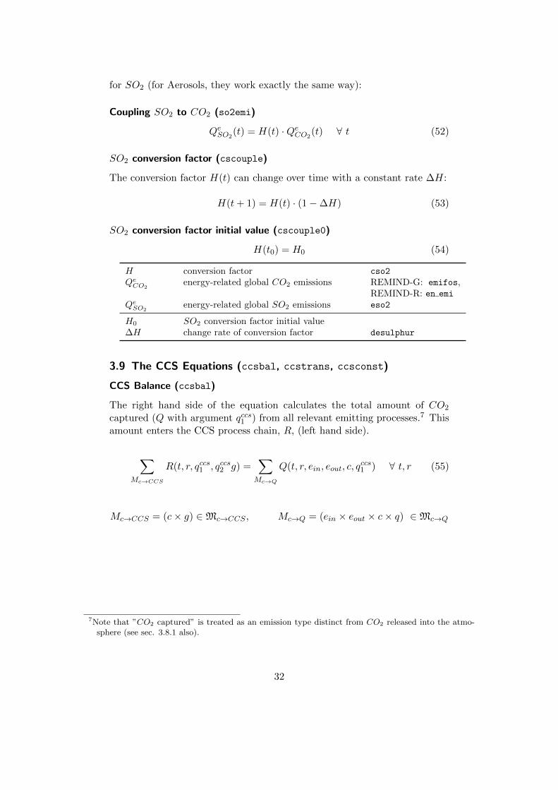
for SO2 (for Aerosols, they work exactly the same way):

Coupling SO2 to CO2 (so2emi)

QeSO2(t) = H(t) ·QeCO2

(t) ∀ t (52)

SO2 conversion factor (cscouple)

The conversion factor H(t) can change over time with a constant rate ∆H:

H(t+ 1) = H(t) · (1−∆H) (53)

SO2 conversion factor initial value (cscouple0)

H(t0) = H0 (54)

H conversion factor cso2

QeCO2energy-related global CO2 emissions REMIND-G: emifos,

REMIND-R: en emi

QeSO2energy-related global SO2 emissions eso2

H0 SO2 conversion factor initial value∆H change rate of conversion factor desulphur

3.9 The CCS Equations (ccsbal, ccstrans, ccsconst)

CCS Balance (ccsbal)

The right hand side of the equation calculates the total amount of CO2

captured (Q with argument qccs1 ) from all relevant emitting processes.7 Thisamount enters the CCS process chain, R, (left hand side).

∑Mc→CCS

R(t, r, qccs1 , qccs2 g) =∑Mc→Q

Q(t, r, ein, eout, c, qccs1 ) ∀ t, r (55)

Mc→CCS = (c× g) ∈Mc→CCS , Mc→Q = (ein × eout × c× q) ∈Mc→Q

7Note that ”CO2 captured” is treated as an emission type distinct from CO2 released into the atmo-sphere (see sec. 3.8.1 also).

32

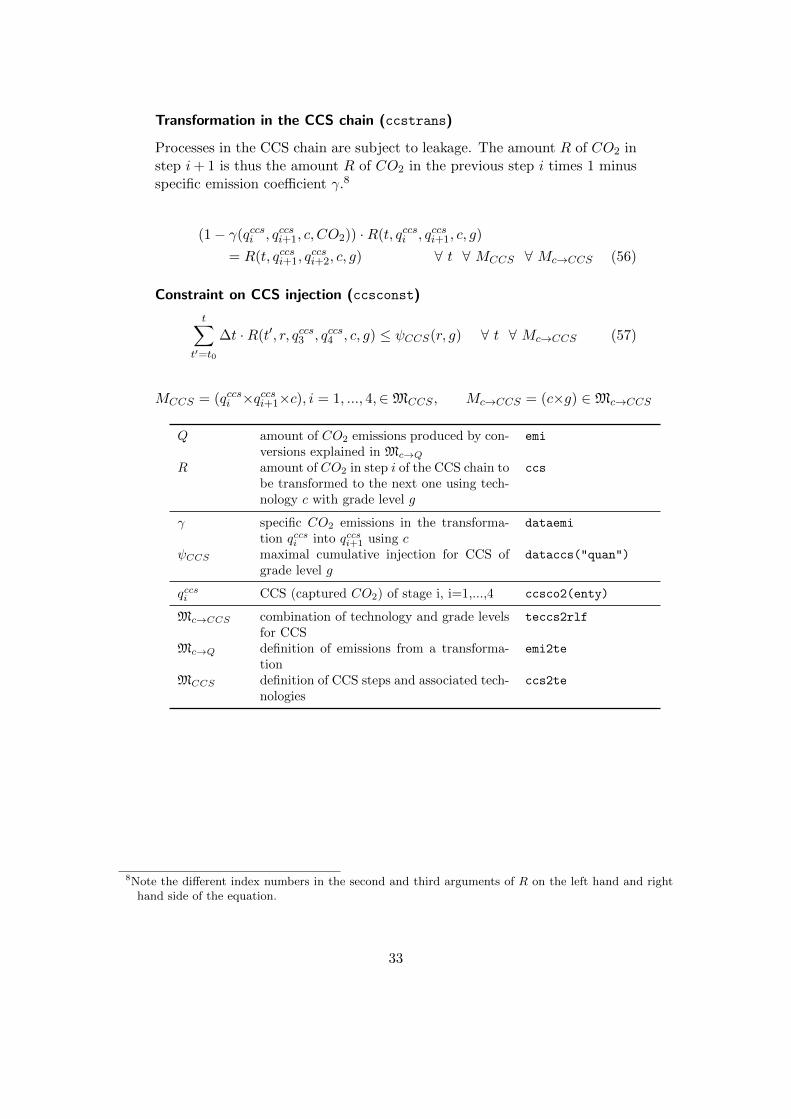
Transformation in the CCS chain (ccstrans)

Processes in the CCS chain are subject to leakage. The amount R of CO2 instep i+ 1 is thus the amount R of CO2 in the previous step i times 1 minusspecific emission coefficient γ.8

(1− γ(qccsi , qccsi+1, c, CO2)) ·R(t, qccsi , qccsi+1, c, g)

= R(t, qccsi+1, qccsi+2, c, g) ∀ t ∀ MCCS ∀ Mc→CCS (56)

Constraint on CCS injection (ccsconst)

t∑t′=t0

∆t ·R(t′, r, qccs3 , qccs4 , c, g) ≤ ψCCS(r, g) ∀ t ∀ Mc→CCS (57)

MCCS = (qccsi ×qccsi+1×c), i = 1, ..., 4,∈MCCS , Mc→CCS = (c×g) ∈Mc→CCS

Q amount of CO2 emissions produced by con-versions explained in Mc→Q

emi

R amount of CO2 in step i of the CCS chain tobe transformed to the next one using tech-nology c with grade level g

ccs

γ specific CO2 emissions in the transforma-tion qccsi into qccsi+1 using c

dataemi

ψCCS maximal cumulative injection for CCS ofgrade level g

dataccs("quan")



teccs2rlf


emi2te


ccs2te

8Note the different index numbers in the second and third arguments of R on the left hand and righthand side of the equation.

33

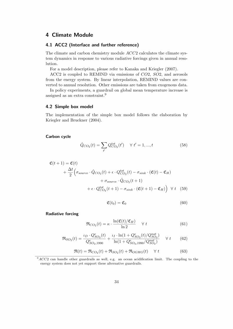
4 Climate Module

4.1 ACC2 (Interface and further reference)

The climate and carbon chemistry module ACC2 calculates the climate sys-tem dynamics in response to various radiative forcings given in annual reso-lution.

For a model description, please refer to Kanaka and Kriegler (2007).ACC2 is coupled to REMIND via emissions of CO2, SO2, and aerosols

from the energy system. By linear interpolation, REMIND values are con-verted to annual resolution. Other emissions are taken from exogenous data.

In policy experiments, a guardrail on global mean temperature increase isassigned as an extra constraint.9

4.2 Simple box model

The implementation of the simple box model follows the elaboration byKriegler and Bruckner (2004).

Carbon cycle

QCO2(t) =∑t′

QtotCO2(t′) ∀ t′ = 1, ..., t (58)

C(t+ 1) = C(t)

+∆t

2

(σsource · QCO2(t) + ε ·QtotCO2

(t)− σsink · (C(t)− CH)

+ σsource · QCO2(t+ 1)

+ ε ·QtotCO2(t+ 1)− σsink · (C(t+ 1)− CH)

)∀ t (59)

C(t0) = C0 (60)

Radiative forcing

RCO2(t) = κ · ln(C(t)/CH)

ln 2∀ t (61)

RSO2(t) =ιD ·QeSO2

(t)

QeSO2,1990

+ιI · ln(1 +QeSO2

(t)/QnatSO2)

ln(1 +QeSO2,1990/QnatSO2

)∀ t (62)

R(t) = RCO2(t) + RSO2(t) + ROGHG(t) ∀ t (63)

9ACC2 can handle other guardrails as well, e.g. an ocean acidification limit. The coupling to theenergy system does not yet support these alternative guardrails.

34

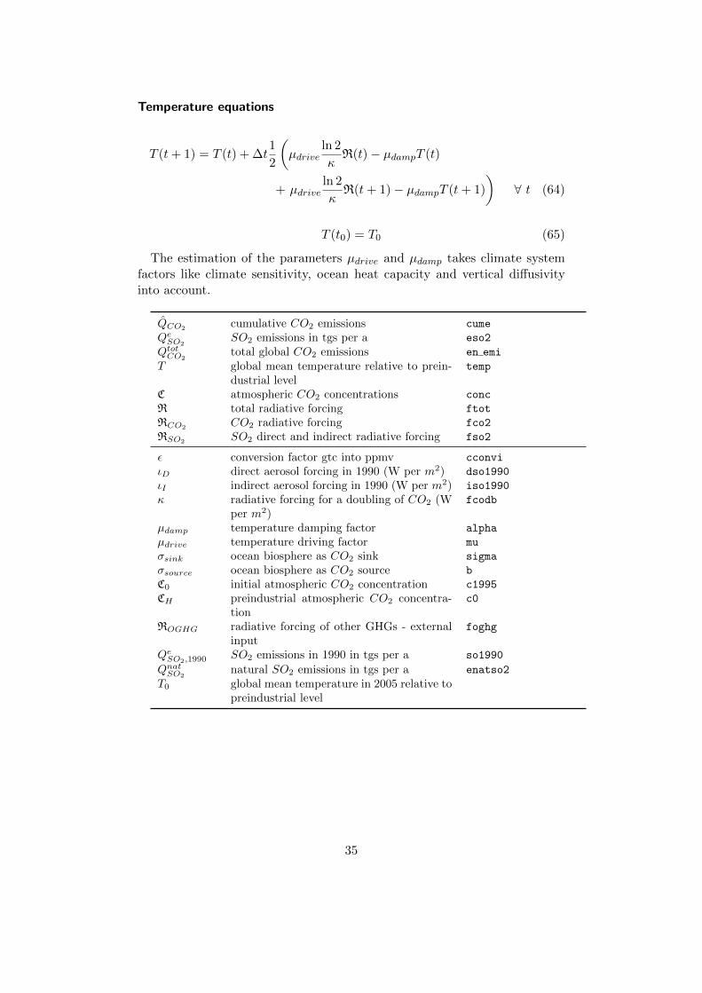
Temperature equations

T (t+ 1) = T (t) + ∆t1

2

(µdrive

ln 2

κR(t)− µdampT (t)

+ µdriveln 2

κR(t+ 1)− µdampT (t+ 1)

)∀ t (64)

T (t0) = T0 (65)

The estimation of the parameters µdrive and µdamp takes climate systemfactors like climate sensitivity, ocean heat capacity and vertical diffusivityinto account.

QCO2 cumulative CO2 emissions cume

QeSO2SO2 emissions in tgs per a eso2


T global mean temperature relative to prein-dustrial level

temp

C atmospheric CO2 concentrations conc

R total radiative forcing ftot

RCO2CO2 radiative forcing fco2

RSO2 SO2 direct and indirect radiative forcing fso2

ε conversion factor gtc into ppmv cconvi

ιD direct aerosol forcing in 1990 (W per m2) dso1990

ιI indirect aerosol forcing in 1990 (W per m2) iso1990

κ radiative forcing for a doubling of CO2 (Wper m2)

fcodb

µdamp temperature damping factor alpha

µdrive temperature driving factor mu

σsink ocean biosphere as CO2 sink sigma

σsource ocean biosphere as CO2 source b

C0 initial atmospheric CO2 concentration c1995

CH preindustrial atmospheric CO2 concentra-tion

c0

ROGHG radiative forcing of other GHGs - externalinput

foghg

QeSO2,1990SO2 emissions in 1990 in tgs per a so1990

QnatSO2natural SO2 emissions in tgs per a enatso2

T0 global mean temperature in 2005 relative topreindustrial level

35

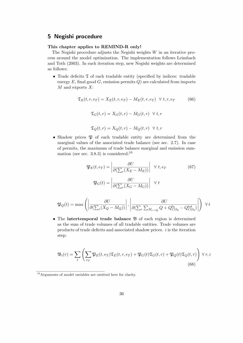
5 Negishi procedure

This chapter applies to REMIND-R only!The Negishi procedure adjusts the Negishi weights W in an iterative pro-

cess around the model optimization. The implementation follows Leimbachand Toth (2003). In each iteration step, new Negishi weights are determinedas follows:

• Trade deficits T of each tradable entity (specified by indices: tradableenergy E, final good G, emission permits Q) are calculated from importsM and exports X:

TE(t, r, eT ) = XE(t, r, eT )−ME(t, r, eT ) ∀ t, r, eT (66)

TG(t, r) = XG(t, r)−MG(t, r) ∀ t, r

TQ(t, r) = XQ(t, r)−MQ(t, r) ∀ t, r

• Shadow prices P of each tradable entity are determined from themarginal values of the associated trade balance (see sec. 2.7). In caseof permits, the maximum of trade balance marginal and emission sum-mation (see sec. 3.8.3) is considered:10

PE(t, eT ) =

∣∣∣∣ ∂U

∂(∑

r(XE −ME))

∣∣∣∣ ∀ t, eT (67)

PG(t) =

∣∣∣∣ ∂U

∂(∑

r(XG −MG))

∣∣∣∣ ∀ t

PQ(t) = max

(∣∣∣∣ ∂U

∂(∑

r(XQ −MQ))

∣∣∣∣ ,∣∣∣∣∣ ∂U

∂(∑

r

∑Mc→Q

Q+QluCO2−QtotCO2

)

∣∣∣∣∣)∀ t

• The intertemporal trade balance B of each region is determinedas the sum of trade volumes of all tradable entities. Trade volumes areproducts of trade deficits and associated shadow prices. i is the iterationstep:

Bi(r) =∑t

(∑eT

PE(t, eT )TE(t, r, eT ) + PG(t)TG(t, r) + PQ(t)TQ(t, r)

)∀ r, i

(68)

10Arguments of model variables are omitted here for clarity.

36

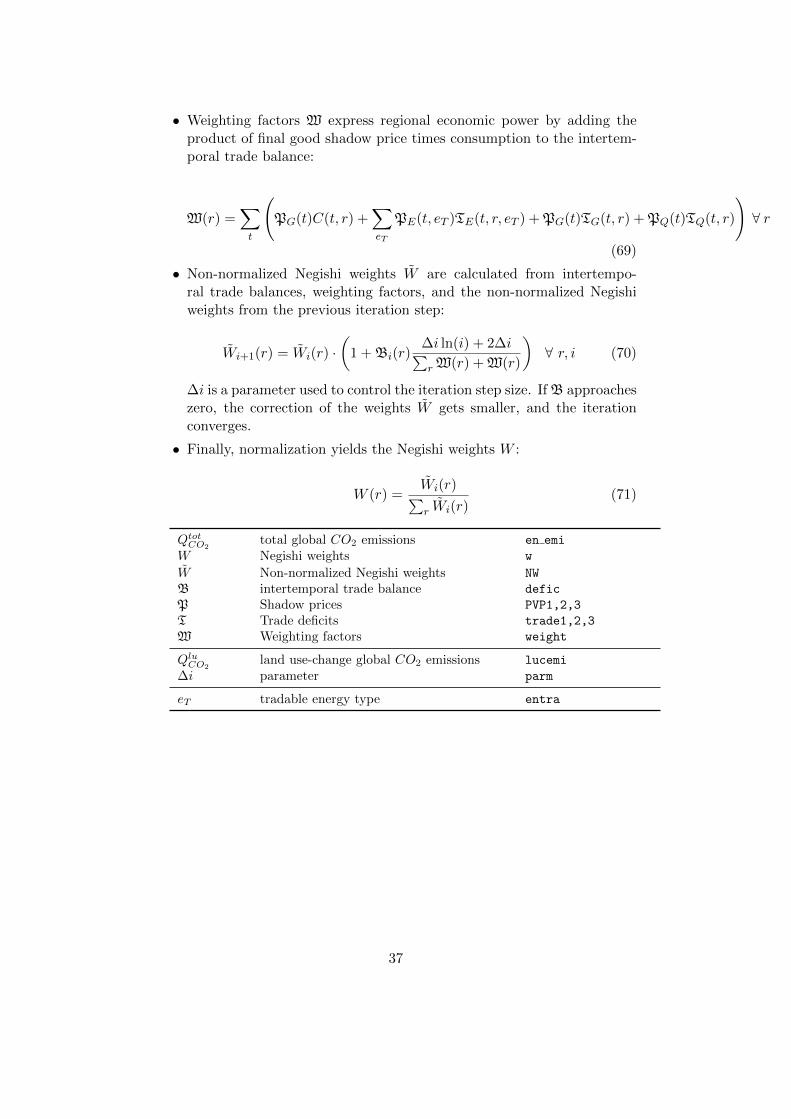
• Weighting factors W express regional economic power by adding theproduct of final good shadow price times consumption to the intertem-poral trade balance:

W(r) =∑t

(PG(t)C(t, r) +

∑eT

PE(t, eT )TE(t, r, eT ) + PG(t)TG(t, r) + PQ(t)TQ(t, r)

)∀ r

(69)

• Non-normalized Negishi weights W are calculated from intertempo-ral trade balances, weighting factors, and the non-normalized Negishiweights from the previous iteration step:

Wi+1(r) = Wi(r) ·(

1 + Bi(r)∆i ln(i) + 2∆i∑rW(r) + W(r)

)∀ r, i (70)

∆i is a parameter used to control the iteration step size. If B approacheszero, the correction of the weights W gets smaller, and the iterationconverges.

• Finally, normalization yields the Negishi weights W :

W (r) =Wi(r)∑r Wi(r)

(71)


W Negishi weights w

W Non-normalized Negishi weights NW

B intertemporal trade balance defic

P Shadow prices PVP1,2,3

T Trade deficits trade1,2,3

W Weighting factors weight

QluCO2land use-change global CO2 emissions lucemi

∆i parameter parm


37

38

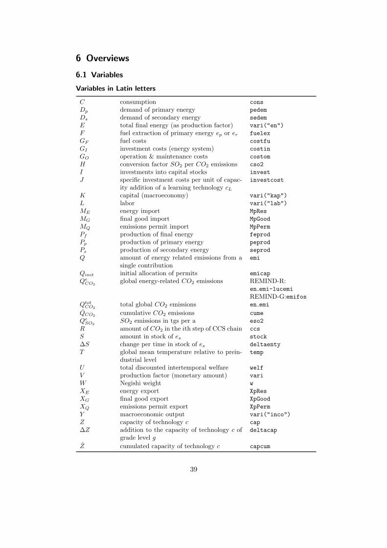
6 Overviews

6.1 Variables

Variables in Latin letters

C consumption cons

Dp demand of primary energy pedem

Ds demand of secondary energy sedem

E total final energy (as production factor) vari("en")

F fuel extraction of primary energy ep or er fuelex

GF fuel costs costfu

GI investment costs (energy system) costin


H conversion factor SO2 per CO2 emissions cso2

I investments into capital stocks invest

J specific investment costs per unit of capac-ity addition of a learning technology cL

investcost

K capital (macroeconomy) vari("kap")

L labor vari("lab")

ME energy import MpRes

MG final good import MpGood

MQ emissions permit import MpPerm




Q amount of energy related emissions from asingle contribution

emi

Qinit initial allocation of permits emicap

QeCO2global energy-related CO2 emissions REMIND-R:

en emi-lucemi

REMIND-G:emifosQtotCO2

total global CO2 emissions en emi

QCO2cumulative CO2 emissions cume

QeSO2SO2 emissions in tgs per a eso2

R amount of CO2 in the ith step of CCS chain ccs

S amount in stock of es stock

∆S change per time in stock of es deltaenty

T global mean temperature relative to prein-dustrial level

temp

U total discounted intertemporal welfare welf

V production factor (monetary amount) vari

W Negishi weight w

XE energy export XpRes

XG final good export XpGood

XQ emissions permit export XpPerm




deltacap

Z cumulated capacity of technology c capcum

39

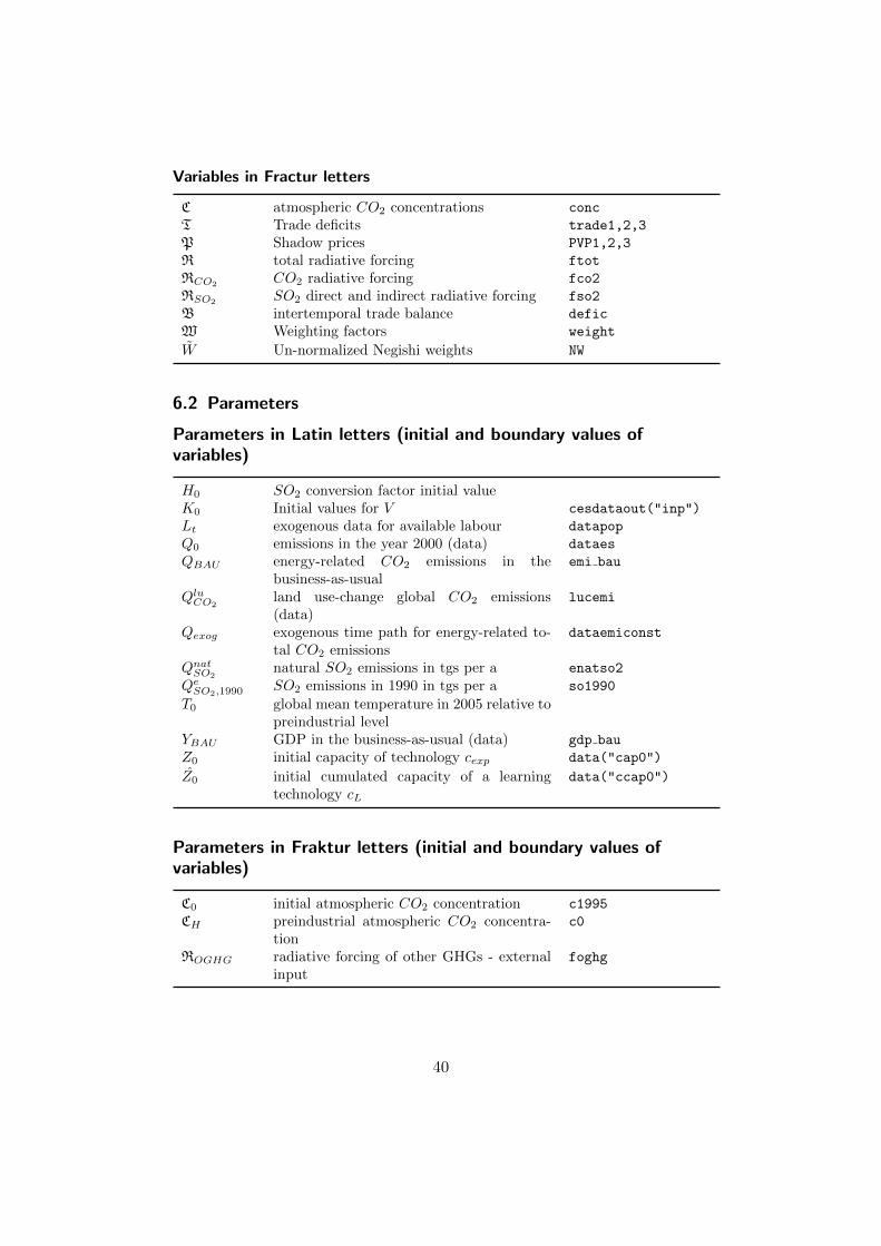
Variables in Fractur letters

C atmospheric CO2 concentrations conc

T Trade deficits trade1,2,3

P Shadow prices PVP1,2,3

R total radiative forcing ftot

RCO2CO2 radiative forcing fco2

RSO2SO2 direct and indirect radiative forcing fso2

B intertemporal trade balance defic

W Weighting factors weight

W Un-normalized Negishi weights NW

6.2 Parameters

Parameters in Latin letters (initial and boundary values ofvariables)

H0 SO2 conversion factor initial valueK0 Initial values for V cesdataout("inp")

Lt exogenous data for available labour datapop

Q0 emissions in the year 2000 (data) dataes

QBAU energy-related CO2 emissions in thebusiness-as-usual

emi bau

QluCO2land use-change global CO2 emissions(data)

lucemi

Qexog exogenous time path for energy-related to-tal CO2 emissions

dataemiconst

QnatSO2natural SO2 emissions in tgs per a enatso2

QeSO2,1990SO2 emissions in 1990 in tgs per a so1990

T0 global mean temperature in 2005 relative topreindustrial level

YBAU GDP in the business-as-usual (data) gdp bau

Z0 initial capacity of technology cexp data("cap0")

Z0 initial cumulated capacity of a learningtechnology cL

data("ccap0")

Parameters in Fraktur letters (initial and boundary values ofvariables)

C0 initial atmospheric CO2 concentration c1995

CH preindustrial atmospheric CO2 concentra-tion

c0

ROGHG radiative forcing of other GHGs - externalinput

foghg

40

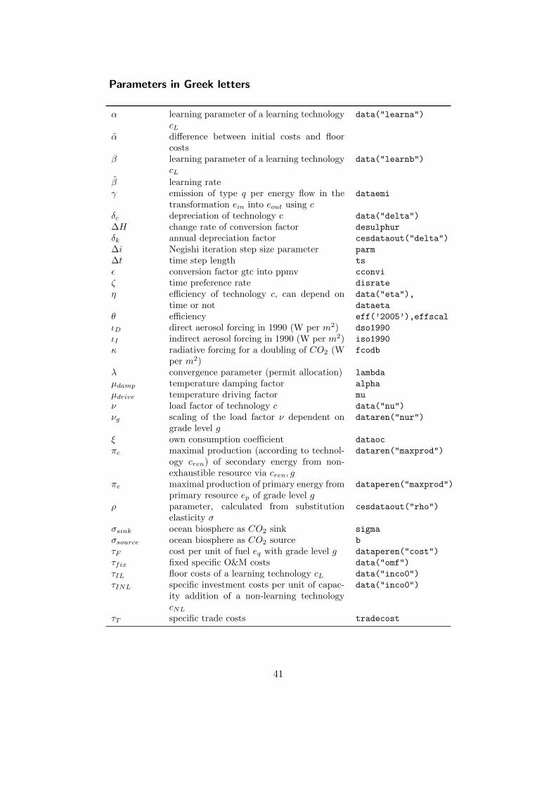
Parameters in Greek letters

α learning parameter of a learning technologycL

data("learna")

α difference between initial costs and floorcosts

β learning parameter of a learning technologycL

data("learnb")

β learning rateγ emission of type q per energy flow in the

transformation ein into eout using cdataemi

δc depreciation of technology c data("delta")

∆H change rate of conversion factor desulphur

δk annual depreciation factor cesdataout("delta")

∆i Negishi iteration step size parameter parm


ε conversion factor gtc into ppmv cconvi

ζ time preference rate disrate


data("eta"),

dataeta

θ efficiency eff(’2005’),effscal

ιD direct aerosol forcing in 1990 (W per m2) dso1990

ιI indirect aerosol forcing in 1990 (W per m2) iso1990

κ radiative forcing for a doubling of CO2 (Wper m2)

fcodb

λ convergence parameter (permit allocation) lambda

µdamp temperature damping factor alpha

µdrive temperature driving factor mu



dataren("nur")


πc maximal production (according to technol-ogy cren) of secondary energy from non-exhaustible resource via cren, g

dataren("maxprod")

πe maximal production of primary energy fromprimary resource ep of grade level g

dataperen("maxprod")

ρ parameter, calculated from substitutionelasticity σ

cesdataout("rho")

σsink ocean biosphere as CO2 sink sigma

σsource ocean biosphere as CO2 source b

τF cost per unit of fuel eq with grade level g dataperen("cost")

τfix fixed specific O&M costs data("omf")

τIL floor costs of a learning technology cL data("inco0")


data("inco0")

τT specific trade costs tradecost

41

τvar variable specific O&M costs data("omv")

φ total factor productivity cesdataout("phi")

χi parameters to characterize the exhaustiblefuel cost curve (i=1,2,3,4)

datarog

ψCCS maximal cumulative injection for CCS ofgrade level g

dataccs("quan")

ψS capacity of stock of quantity s stockmax


datacap("omeg")

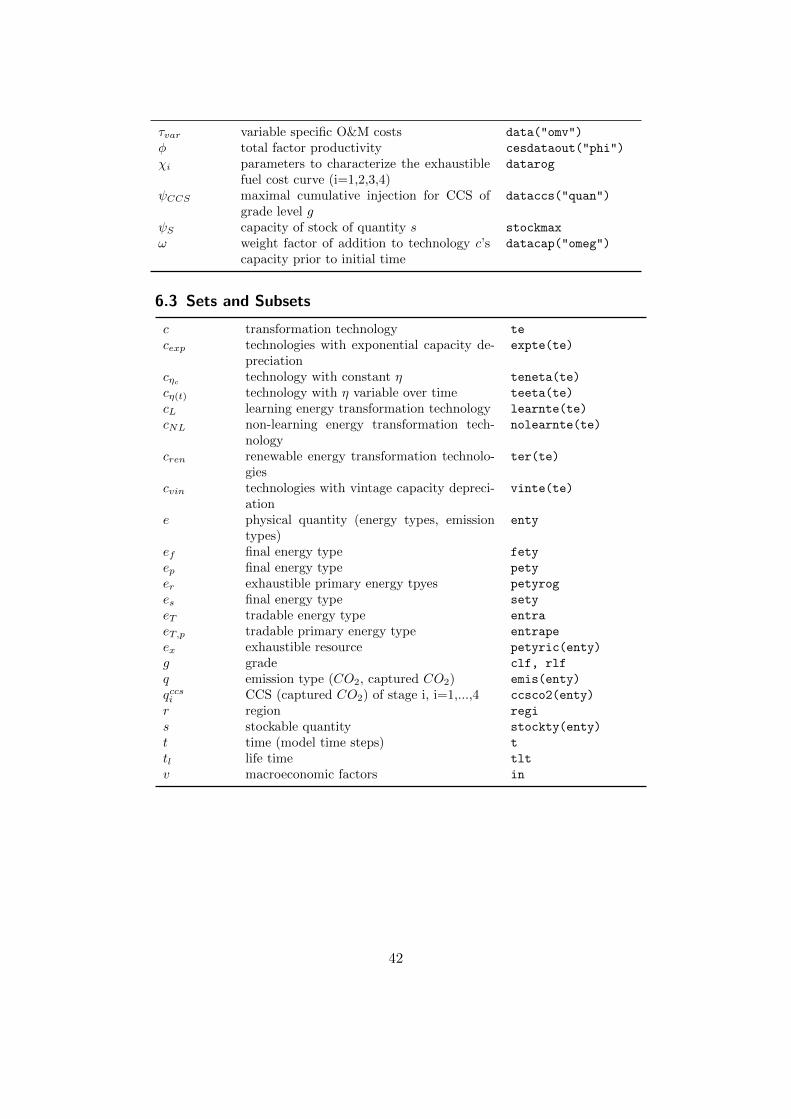
6.3 Sets and Subsets

c transformation technology te

cexp technologies with exponential capacity de-preciation

expte(te)

cηc technology with constant η teneta(te)

cη(t) technology with η variable over time teeta(te)



nolearnte(te)

cren renewable energy transformation technolo-gies

ter(te)

cvin technologies with vintage capacity depreci-ation

vinte(te)

e physical quantity (energy types, emissiontypes)

enty

ef final energy type fety

ep final energy type pety

er exhaustible primary energy tpyes petyrog

es final energy type sety


eT,p tradable primary energy type entrape

ex exhaustible resource petyric(enty)

g grade clf, rlf

q emission type (CO2, captured CO2) emis(enty)


r region regi

s stockable quantity stockty(enty)

t time (model time steps) t

tl life time tlt

v macroeconomic factors in

42

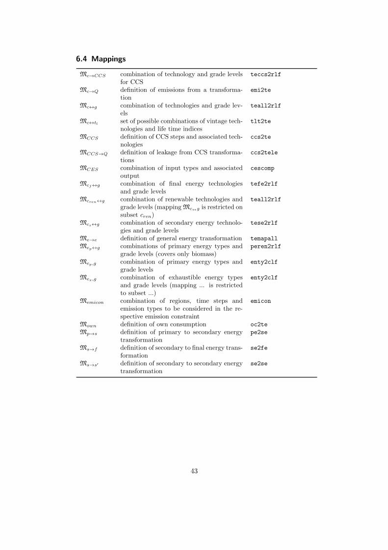
6.4 Mappings


teccs2rlf


emi2te


teall2rlf


tlt2te


ccs2te

MCCS→Q definition of leakage from CCS transforma-tions

ccs2tele

MCES combination of input types and associatedoutput

cescomp

Mcf↔g combination of final energy technologiesand grade levels

tefe2rlf

Mcren↔g combination of renewable technologies andgrade levels (mapping Mc↔g is restricted onsubset cren)

teall2rlf


tese2rlf


Mep↔g combinations of primary energy types andgrade levels (covers only biomass)

peren2rlf

Mep,g combination of primary energy types andgrade levels

enty2clf

Mex,g combination of exhaustible energy typesand grade levels (mapping ... is restrictedto subset ...)

enty2clf

Memicon combination of regions, time steps andemission types to be considered in the re-spective emission constraint

emicon



pe2se


se2fe


se2se

43

7 Literature

Kanaka and Kriegler (2007): Tanaka, K., Kriegler, E. (2007): Aggre-gated Carbon Cycle, Atmospheric Chemistry, and Climate Model (ACC2).Reports on Earth System Science, 40. Max-Planck-Institute of Meteorology,Hamburg (Germany).

Kriegler and Bruckner (2004): Kriegler, E., Bruckner, T. (2004):Sensitivity of emissions corridors for the 21st century. Climatic Change 66,345-387.

Leimbach and Toth (2003): Leimbach, M., Toth, F. (2003): Economicdevelopment and emission control over the long term: The ICLIPS aggre-gated economic model. Climatic Change, 56, 139-165.

44

Documents

Remind: the equations · fraktur, e.g. T. (Please note an exception: M is used for mappings.) Parametersare written as Greek letters. Exception: initial and bound-ary conditions on