Reliability Assessment of Tower Crane Structural Members-G03178 Idzuari Azli

2016

Kamilan, Idzuari Azli

MSc Asset Management & Maintenance

1/2/2016

Reliability Assessment of Tower Crane Structural Members

Reliability Assessment of Tower Crane Structural Members 2016

1 | P a g e

Table of Contents 1.0 Introduction ....................................................................................................................................... 2

2.0 General Reliability Methods .............................................................................................................. 3

2.1 Time-Dependent Reliability ........................................................................................................... 3

2.2 Stress-Strength Interference Methods .......................................................................................... 4

2.3 Reliability Index ............................................................................................................................. 5

2.4 Monte Carlo Simulations ............................................................................................................... 7

2.5 Stochastic Sensitivity Analysis ....................................................................................................... 8

3.0 Conclusion ....................................................................................................................................... 11

4.0 Bibliography ..................................................................................................................................... 12


2 | P a g e

1.0 Introduction

Crane structural members, which are mainly made of steel plates and beams connected by welding, are subjected to repeated operating loads. Intensive crane use usually stems from the need to minimize the amount of time required to complete a construction by maximizing the efficiency of equipments and teams. Therefore, the fatigue design of tower cranes must be accounted for. The probabilistic approaches represent promising methods enabling to quantify and manage the reliability of crane structural members. These methods require the characterization of the uncertainties related to the fatigue phenomenon of welded joints and fatigue operating loads. Thus, this project paper aims to introduce the concepts commonly used for modeling fatigue strength and operating loads on one hand, and to define the basic principles used in reliability analyses, on the other hand. Section 2.0 deals with the notions related to reliability approaches in general. After introducing the definitions of the time-dependent reliability, the Stress-Strength Interference (SSI) method is outlined. This section also describes the relationship between the failure probability and the reliability index, and presents the simplest method allowing to assess them, namely the Monte Carlo simulations. Finally, this section discusses a global sensitivity analysis procedure. Considering a given mathematical model, the Sobol’s method aims at quantifying the sensitivity indices reflecting the impact of the variability of each input parameters on the mechanical response.


3 | P a g e

2.0 General Reliability Methods

The main objective of this project paper is to develop a comprehensive probabilistic procedure enabling to assess the reliability of crane members according to their operating time. For this purpose, the basic principles of reliability methods needed to achieve this essential task are discussed in this section. The time-dependent reliability is first introduced in section 2.1 and, section 2.2 presents the so-called stress-strength interference (SSI) methods. Following this, section 2.3 gives definitions related to the reliability index, and section 2.4 describes the Monte Carlo simulations. Lastly, the Sobol sensitivity analysis method is outlined in section 2.5.

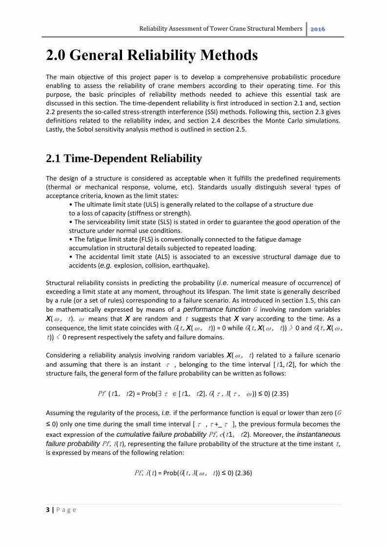
2.1 Time-Dependent Reliability

The design of a structure is considered as acceptable when it fulfills the predefined requirements (thermal or mechanical response, volume, etc). Standards usually distinguish several types of acceptance criteria, known as the limit states:

• The ultimate limit state (ULS) is generally related to the collapse of a structure due to a loss of capacity (stiffness or strength). • The serviceability limit state (SLS) is stated in order to guarantee the good operation of the structure under normal use conditions. • The fatigue limit state (FLS) is conventionally connected to the fatigue damage accumulation in structural details subjected to repeated loading. • The accidental limit state (ALS) is associated to an excessive structural damage due to accidents (e.g. explosion, collision, earthquake).

Structural reliability consists in predicting the probability (i.e. numerical measure of occurrence) of exceeding a limit state at any moment, throughout its lifespan. The limit state is generally described by a rule (or a set of rules) corresponding to a failure scenario. As introduced in section 1.5, this can

be mathematically expressed by means of a performance function G involving random variables

X(ω, t). ω means that X are random and t suggests that X vary according to the time. As a

consequence, the limit state coincides with G(t,X(ω, t)) = 0 while G(t,X(ω, t)) > 0 and G(t,X(ω, t)) < 0 represent respectively the safety and failure domains.

Considering a reliability analysis involving random variables X(ω, t) related to a failure scenario

and assuming that there is an instant τ , belonging to the time interval [t1,t2], for which the structure fails, the general form of the failure probability can be written as follows:

Pf (t1, t2) = Prob(∃τ ∈ [t1, t2],G(τ,X(τ, ω)) ≤ 0) (2.35)

Assuming the regularity of the process, i.e. if the performance function is equal or lower than zero (G

≤ 0) only one time during the small time interval [τ ,τ+_τ ], the previous formula becomes the

exact expression of the cumulative failure probability Pf,c(t1, t2). Moreover, the instantaneous

failure probability Pf,i(t), representing the failure probability of the structure at the time instant t, is expressed by means of the following relation:

Pf,i(t) = Prob(G(t,X(ω, t)) ≤ 0) (2.36)


4 | P a g e

As shown by Céline Andrieu-Renaud during her PhD [2], Pf,i and Pf,c(t1, t2) are theoretically

different, excepted if the performance function G decreases monotonically according to t. This may occur for instance for degradation processes such as corrosion and fatigue cracking. Once a crack appears, fatigue cracking leads to the degradation of material characteristics until a potential strengthening (re-welding, etc) of the structure. Therefore, in the case of a performance function

strictly decreasing until a time t < ∞, the instantaneous failure probability is identical to the

cumulative failure probability:

Pf,i(t) = Pf,c(0, t) (2.37)

Only the initiation of macroscopic weld toe cracks is considered in this work, which leads to assume that the resistance of crane welded details is not supposed to evolve with time. Thus, given that the crane member fatigue damage induced by cyclic loading increases with operating time, the margin between the resistance and the stress of the structure decreases monotonically. Consequently, the probabilities calculated in the following correspond either to instantaneous or cumulative failure

probabilities and are denoted Pf . Additionally, for the sake of clarity, the notation ω, indicating the randomness inherent to the variables, is omitted in the following.

2.2 Stress-Strength Interference Methods

In industrial context, the most simple failure scenario consists in comparing two random variables

related respectively to a stress S (demand) on one hand and a strength R (supply) on the other hand. In other words, a structure is safe in accordance with a failure criterion if, at any time, the applied

stress remains below the strength of the component. Methods based on the separation of S and R are named SSI (Stress-Strength Interference) methods. As shown in section 2.1, S and R can

be time-variant depending on the physical behavior of the studied structure. For instance, R = R(t) if

the corrosion of a metallic component is considered or S = S(t) if a structure is subjected to random

loading. By the way, the performance function G is regularly expressed as a combination of

progressive degradation process R(t) and a random loading S(t): G(t) = S(t)−R(t).

The failure criterion considered in this thesis concerns exclusively the initiation of a macroscopic crack at weld toe. Thus, the material characteristics decrease induced by crack propagation is not considered here. Furthermore, crane structural assemblies are painted in order to prevent corrosion problems. As a result, fatigue strength of crane welded assemblies is supposed to be time-independent. By contrast, as seen in section 1.4, the construction site duration and the time between two jobs imply uncertainties concerning crane use (i.e. structural loading) leading to the conclusion

that crane member loading is highly time-dependent. Hence, the performance function G corresponding to the reliability method presented in this thesis is expressed as follows:

G(t) = R − S(t) (2.38)


5 | P a g e

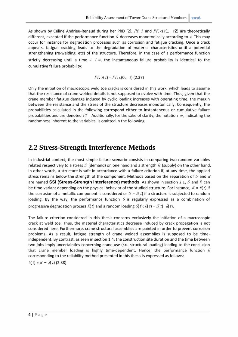
Figure 2.1 – Stress-strength interference method.

As depicted in Figure 2.1 for the case of two Gaussian distributions, the reliability of a crane

structural member can be assessed by characterizing two PDFs related respectively to the stress S(t)

and the strength R. Assuming that these distributions can be determined and are independent, the

failure probability Pf (t) = Prob(G(t) ≤ 0) or equivalently the reliability R(t), depending on operating

time t, is assessed as follows:

where fS and FR are respectively the stress PDF and the strength CDF. SSI methods assume that stress and strength distributions are statistically independent which is not the case in some situations. A second assumption highlighted by Echard et al. [3] lies in the fact that these distributions cannot be fully observed. Therefore, reliability results are very sensitive to the PDF models chosen to fit experimental data. Concerning tower cranes, the intrinsic fatigue strength of crane members is independent of loading history. The first assumption is therefore verified and, provided that the stress and strength PDFs can be fully determined, the stress-strength interference method can be used.

2.3 Reliability Index

Rather than talking about failure probability, it is sometimes convenient to use a dimensionless measure which reflects the reliability of a structure, namely the reliability index. Cornell [4] proposed in 1970 to define the reliability index as the inverse of the coefficient of variation of the

margin Z = R − S:

For instance, concerning the two independent Gaussian distributions presented in section 2.2, the previous formula becomes:


6 | P a g e

Although the Cornell reliability index seems to be convenient in some simple situations (e.g.

Gaussian distributions and linear limit state), this index is sometimes difficult to use because of its lack of generality. In fact, the most general form of the reliability index was given by Hasofer and Lind in 1974 [5]. They proposed to convert random variables from the physical space to a space of standardized independent Gaussian variables (having zero mean and unit variance) by introducing an

isoprobabilistic transformation T. Thus, the method consists in converting independent physical random variables X (of realizations x) into independent standard Gaussian variables U (of realizations u) by writing the mathematical equality of CDFs:

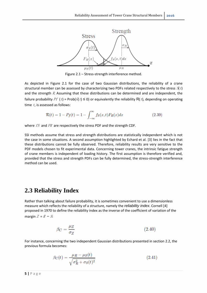
where _ refers to the standard Gaussian CDF. Thereafter, as seen in figure 2.2, the performance

function G is transformed into H in the standardized space, i.e. H(U) . Hence, the

Hasofer-Lind reliability index β corresponds to the minimum distance between the origin and the failure domain:

β = βHL = √utu under the constraint H(u) ≤ 0 (2.43)

In the case of two independent Gaussian distributions and linear limit state as presented before, the Hasofer-Lind and Cornell reliability indexes are equivalent and derived from equation (2.41).

Furthermore, when an analytical expression of R exists, β derives directly from R. Thus,

remembering the time-dependent reliability R(t) expression given in section 2.2, this leads to:

β(t) = −_−1 (1 − R(t)) (2.44)

If no analytical expression exists for R, the reliability index has to be quantified by means of a

numerical method such as Monte Carlo simulations presented in the following section. More details concerning the reliability index can be found in the book of M. Lemaire [1].

Figure 2.2 – Illustration of an isoprobabilistic transformation.


7 | P a g e

2.4 Monte Carlo Simulations

As shown in section 2.1, the failure probability reads:

Pf = Prob(G(X) ≤ 0) (2.45)

By introducing the joint probability density function fX(x), Monte Carlo simulations

consist in performing random sampling of variables X in the whole physical space in order to evaluate the following integral:

where Df is the failure domain. By using the isoprobabilistic transformation T, the previous integral is expressed in the standardized space, leading to recast the failure probability as:

where φn is the joint standard Gaussian PDF. As detailed in the book of Lemaire [6], the

introduction of the indicator function IDf (u) = {1 if H(u) ≤ 0 and 0 otherwise} enables

to rewrite the previous integral as follows:

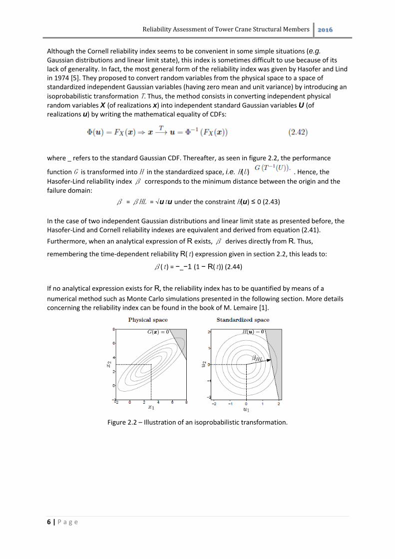
Figure 2.3 – Illustration of Monte Carlo simulations in the case of two standard Gaussian variables.

Gray points mean that the realizations of U1 and U2 are located in the safe domain while the black points mean that they are located in the failure domain. Thus, the failure probability defined in equation 2.48 can be approximated as:

where E[.] is the mathematical expectation and NMC is the number of Monte Carlo simulations.


8 | P a g e

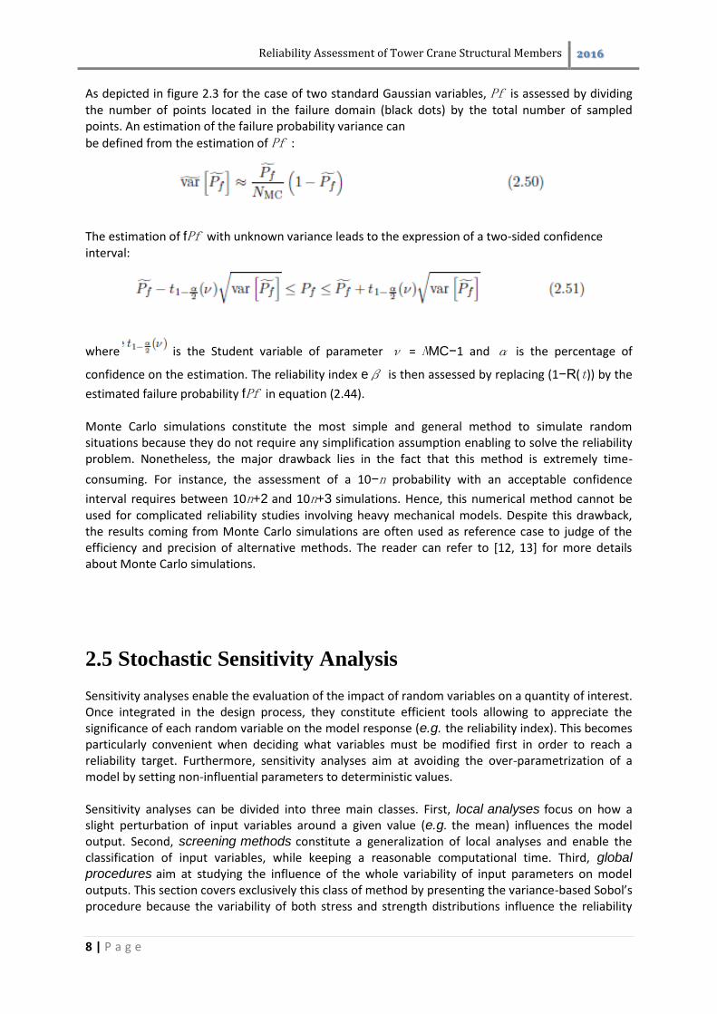
As depicted in figure 2.3 for the case of two standard Gaussian variables, Pf is assessed by dividing the number of points located in the failure domain (black dots) by the total number of sampled points. An estimation of the failure probability variance can

be defined from the estimation of Pf :

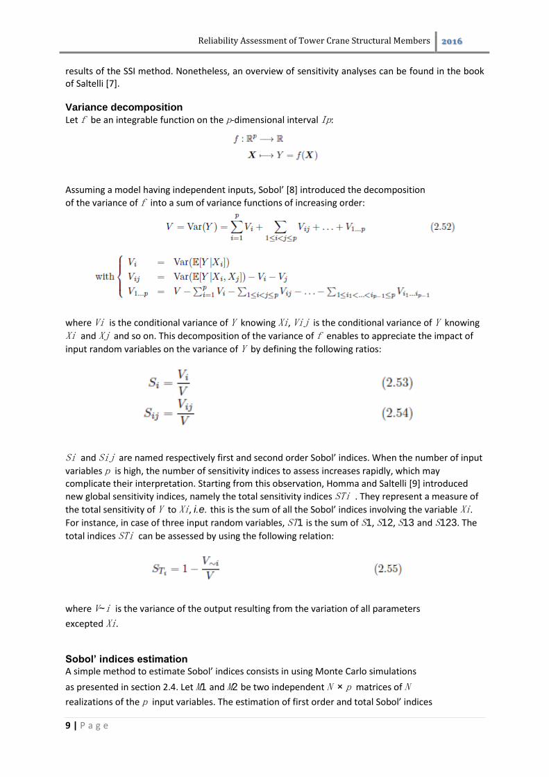
The estimation of fPf with unknown variance leads to the expression of a two-sided confidence interval:

where is the Student variable of parameter ν = NMC−1 and α is the percentage of

confidence on the estimation. The reliability index eβ is then assessed by replacing (1−R(t)) by the

estimated failure probability fPf in equation (2.44). Monte Carlo simulations constitute the most simple and general method to simulate random situations because they do not require any simplification assumption enabling to solve the reliability problem. Nonetheless, the major drawback lies in the fact that this method is extremely time-

consuming. For instance, the assessment of a 10−n probability with an acceptable confidence

interval requires between 10n+2 and 10n+3 simulations. Hence, this numerical method cannot be used for complicated reliability studies involving heavy mechanical models. Despite this drawback, the results coming from Monte Carlo simulations are often used as reference case to judge of the efficiency and precision of alternative methods. The reader can refer to [12, 13] for more details about Monte Carlo simulations.

2.5 Stochastic Sensitivity Analysis

Sensitivity analyses enable the evaluation of the impact of random variables on a quantity of interest. Once integrated in the design process, they constitute efficient tools allowing to appreciate the significance of each random variable on the model response (e.g. the reliability index). This becomes particularly convenient when deciding what variables must be modified first in order to reach a reliability target. Furthermore, sensitivity analyses aim at avoiding the over-parametrization of a model by setting non-influential parameters to deterministic values. Sensitivity analyses can be divided into three main classes. First, local analyses focus on how a slight perturbation of input variables around a given value (e.g. the mean) influences the model output. Second, screening methods constitute a generalization of local analyses and enable the classification of input variables, while keeping a reasonable computational time. Third, global

procedures aim at studying the influence of the whole variability of input parameters on model outputs. This section covers exclusively this class of method by presenting the variance-based Sobol’s procedure because the variability of both stress and strength distributions influence the reliability


9 | P a g e

results of the SSI method. Nonetheless, an overview of sensitivity analyses can be found in the book of Saltelli [7]. Variance decomposition

Let f be an integrable function on the p-dimensional interval Ip:

Assuming a model having independent inputs, Sobol’ [8] introduced the decomposition

of the variance of f into a sum of variance functions of increasing order:

where Vi is the conditional variance of Y knowing Xi, Vij is the conditional variance of Y knowing

Xi and Xj and so on. This decomposition of the variance of f enables to appreciate the impact of

input random variables on the variance of Y by defining the following ratios:

Si and Sij are named respectively first and second order Sobol’ indices. When the number of input

variables p is high, the number of sensitivity indices to assess increases rapidly, which may complicate their interpretation. Starting from this observation, Homma and Saltelli [9] introduced

new global sensitivity indices, namely the total sensitivity indices STi . They represent a measure of

the total sensitivity of Y to Xi, i.e. this is the sum of all the Sobol’ indices involving the variable Xi.

For instance, in case of three input random variables, ST1 is the sum of S1, S12, S13 and S123. The

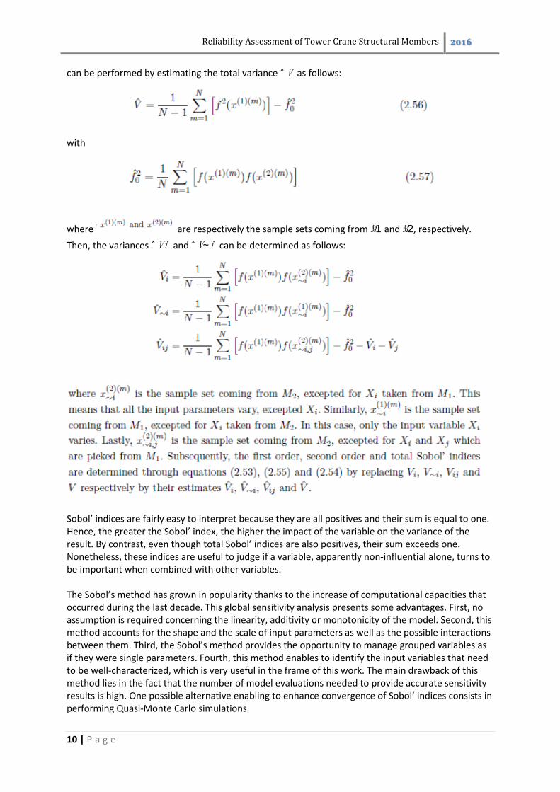
total indices STi can be assessed by using the following relation:

where V∼i is the variance of the output resulting from the variation of all parameters

excepted Xi. Sobol’ indices estimation

A simple method to estimate Sobol’ indices consists in using Monte Carlo simulations

as presented in section 2.4. Let M1 and M2 be two independent N × p matrices of N

realizations of the p input variables. The estimation of first order and total Sobol’ indices


10 | P a g e

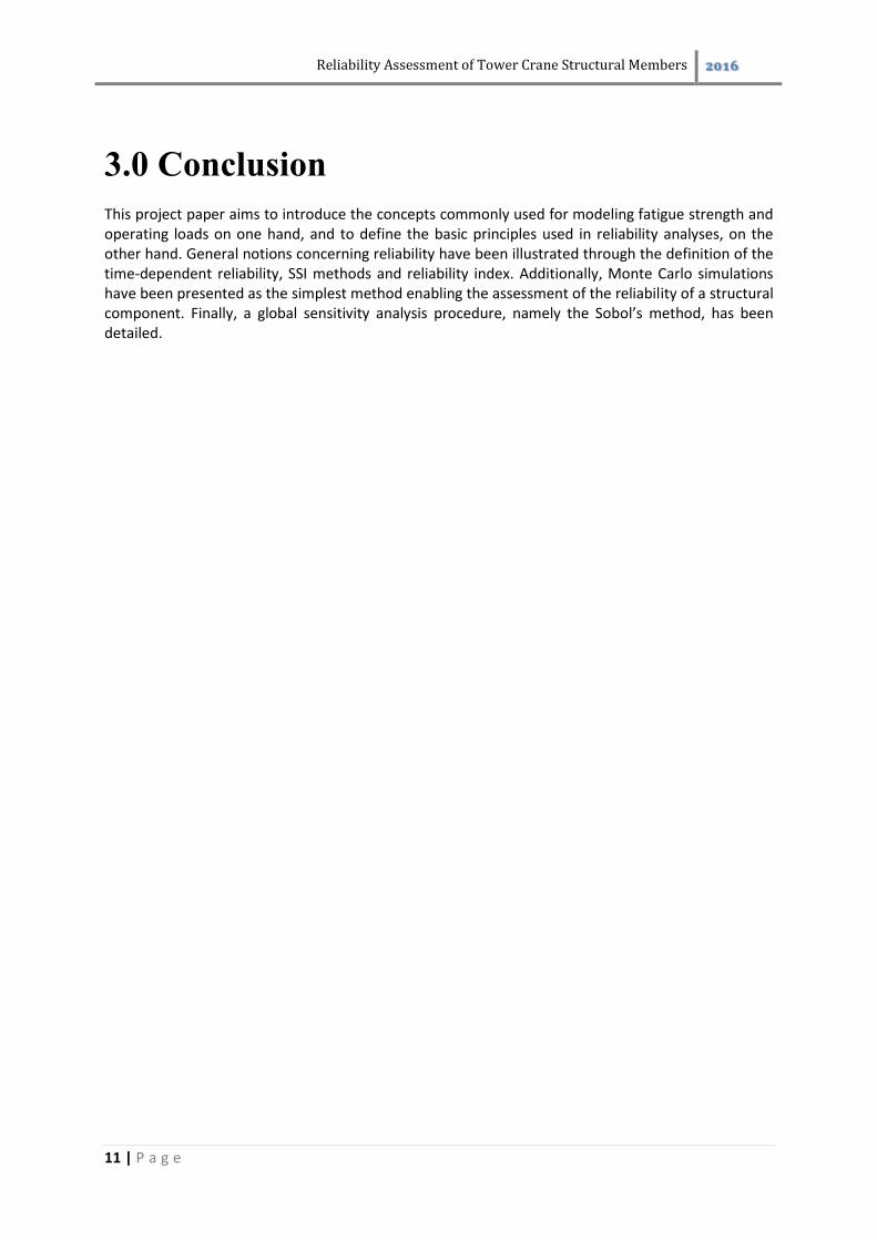
can be performed by estimating the total variance ˆ V as follows:

with

where are respectively the sample sets coming from M1 and M2, respectively.

Then, the variances ˆ Vi and ˆ V∼i can be determined as follows:

Sobol’ indices are fairly easy to interpret because they are all positives and their sum is equal to one. Hence, the greater the Sobol’ index, the higher the impact of the variable on the variance of the result. By contrast, even though total Sobol’ indices are also positives, their sum exceeds one. Nonetheless, these indices are useful to judge if a variable, apparently non-influential alone, turns to be important when combined with other variables. The Sobol’s method has grown in popularity thanks to the increase of computational capacities that occurred during the last decade. This global sensitivity analysis presents some advantages. First, no assumption is required concerning the linearity, additivity or monotonicity of the model. Second, this method accounts for the shape and the scale of input parameters as well as the possible interactions between them. Third, the Sobol’s method provides the opportunity to manage grouped variables as if they were single parameters. Fourth, this method enables to identify the input variables that need to be well-characterized, which is very useful in the frame of this work. The main drawback of this method lies in the fact that the number of model evaluations needed to provide accurate sensitivity results is high. One possible alternative enabling to enhance convergence of Sobol’ indices consists in performing Quasi-Monte Carlo simulations.


11 | P a g e

3.0 Conclusion

This project paper aims to introduce the concepts commonly used for modeling fatigue strength and operating loads on one hand, and to define the basic principles used in reliability analyses, on the other hand. General notions concerning reliability have been illustrated through the definition of the time-dependent reliability, SSI methods and reliability index. Additionally, Monte Carlo simulations have been presented as the simplest method enabling the assessment of the reliability of a structural component. Finally, a global sensitivity analysis procedure, namely the Sobol’s method, has been detailed. Chapt


12 | P a g e

4.0 Bibliography

[1] M. Lemaire, A. Chateauneuf, and J.C. Mitteau. Fiabilité des structures: Couplage mécano-

fiabiliste statique. Hermès Science Publications, 2005. [2] Céline Andrieu-Renaud. Fiabilité mécanique des structures soumises à des phénomènes

physiques dépendant du temps. PhD thesis, PhD thesis, Université Blaise Pascal, Clermont-Ferrand, 2002. [3] B. Echard, N. Gayton, and A. Bignonnet. A reliability analysis method for fatigue design. International Journal of Fatigue, 59:292–300, 2014. [4] JR Benjamin and CA Cornell. Probability, statistics and decision for civil engineers., 1970. [5] A.M. Hasofer and N.C. Lind. Exact and invariant second-moment code format. Journal of the

Engineering Mechanics Division, 100(1):111–121, 1974. [6] M. Lemaire. Structural reliability, volume 84. John Wiley & Sons, 2010. [7] A. Saltelli, K. Chan, and E.M. Scott. Sensitivity Analysis. Wiley paperback series. Wiley, 2009. [8] I. Sobol. Sensitivity estimates for nonlinear mathematical models. Mathematical Modeling &

Computational Experiment, 1:407–414, 1993. [9] T. Homma and A. Saltelli. Importance measures in global sensitivity analysis of nonlinear models. Reliability Engineering & System Safety, 52(1):1 – 17, 1996. doi: http://dx.doi.org/10.1016/0951-8320(96)00002-6.

Documents

Reliability Assessment of Tower Crane Structural Members-G03178 Idzuari Azli