Relative Distribution Methods in Stata - Boston Collegefm · Outline Introduction The Relative Distribution Basic concepts Location and Shape Eﬀects Implementation: The reldist

Relative Distribution Methods in Stata

Ben Jann

ETH Zurich

6th German Stata Users Group Meeting

Berlin, June 27, 2008

Ben Jann (ETH Zurich) Relative Distribution Methods in Stata DSUG 2008 1 / 30

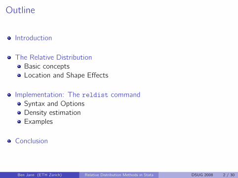
Outline

Introduction

The Relative Distribution

Basic concepts

Location and Shape Effects

Implementation: The reldist command

Syntax and Options

Density estimation

Examples

Conclusion


Introduction

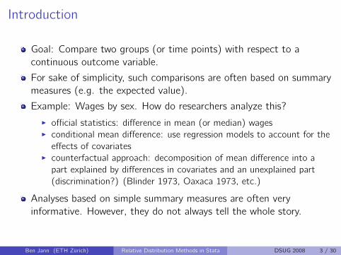
Goal: Compare two groups (or time points) with respect to a

continuous outcome variable.

For sake of simplicity, such comparisons are often based on summary

measures (e.g. the expected value).

Example: Wages by sex. How do researchers analyze this?

I official statistics: difference in mean (or median) wagesI conditional mean difference: use regression models to account for the

effects of covariatesI counterfactual approach: decomposition of mean difference into a

part explained by differences in covariates and an unexplained part

(discrimination?) (Blinder 1973, Oaxaca 1973, etc.)

Analyses based on simple summary measures are often very

informative. However, they do not always tell the whole story.


Introduction

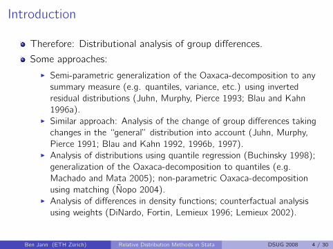
Therefore: Distributional analysis of group differences.

Some approaches:

I Semi-parametric generalization of the Oaxaca-decomposition to any

summary measure (e.g. quantiles, variance, etc.) using inverted

residual distributions (Juhn, Murphy, Pierce 1993; Blau and Kahn

1996a).I Similar approach: Analysis of the change of group differences taking

changes in the “general” distribution into account (Juhn, Murphy,

Pierce 1991; Blau and Kahn 1992, 1996b, 1997).I Analysis of distributions using quantile regression (Buchinsky 1998);

generalization of the Oaxaca-decomposition to quantiles (e.g.

Machado and Mata 2005); non-parametric Oaxaca-decomposition

using matching (Nopo 2004).I Analysis of differences in density functions; counterfactual analysis

using weights (DiNardo, Fortin, Lemieux 1996; Lemieux 2002).


Introduction

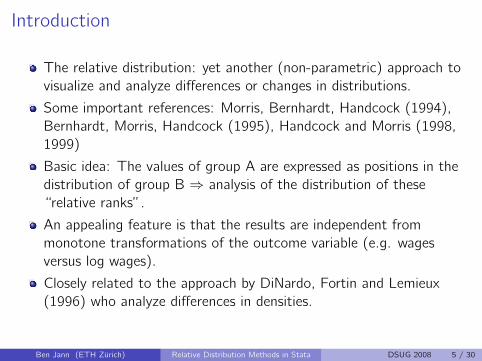
The relative distribution: yet another (non-parametric) approach to

visualize and analyze differences or changes in distributions.

Some important references: Morris, Bernhardt, Handcock (1994),

Bernhardt, Morris, Handcock (1995), Handcock and Morris (1998,

1999)

Basic idea: The values of group A are expressed as positions in the

distribution of group B ⇒ analysis of the distribution of these“relative ranks”.

An appealing feature is that the results are independent from

monotone transformations of the outcome variable (e.g. wages

versus log wages).

Closely related to the approach by DiNardo, Fortin and Lemieux

(1996) who analyze differences in densities.


Relative data: definition

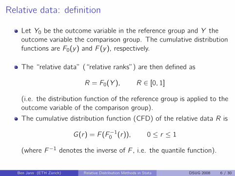
Let Y0 be the outcome variable in the reference group and Y the

outcome variable the comparison group. The cumulative distribution

functions are F0(y) and F (y), respectively.

The “relative data” (“relative ranks”) are then defined as

R = F0(Y ), R ∈ [0, 1]

(i.e. the distribution function of the reference group is applied to the

outcome variable of the comparison group).

The cumulative distribution function (CFD) of the relative data R is

G (r) = F (F−10 (r)), 0 ≤ r ≤ 1

(where F−1 denotes the inverse of F , i.e. the quantile function).


Relative data: definition

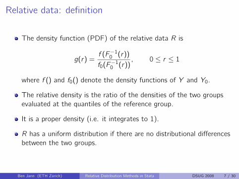
The density function (PDF) of the relative data R is

g(r) =f (F−10 (r))

f0(F−10 (r))

, 0 ≤ r ≤ 1

where f () and f0() denote the density functions of Y and Y0.

The relative density is the ratio of the densities of the two groups

evaluated at the quantiles of the reference group.

It is a proper density (i.e. it integrates to 1).

R has a uniform distribution if there are no distributional differences

between the two groups.


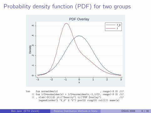
Probability density function (PDF) for two groups

0.1

.2.3

.4.5

Den

sity

−3 −2 −1 0 1 2 3x

f_0f

PDF Overlay

two fun normalden(x) , range(-3 3) ///—— fun 1/2*normalden(x) + 1/2*normalden(x,-1,1/2), range(-3 3) ///—— , xlab(-3(1)3) yti(”Density”) ti(”PDF Overlay”) ///

legend(order(1 ”f˙0” 2 ”f”) pos(2) ring(0) col(1)) name(a)


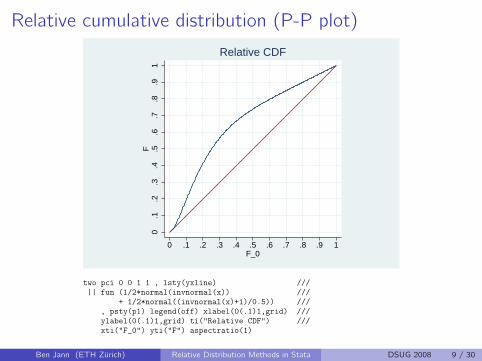
Relative cumulative distribution (P-P plot)

0.1

.2.3

.4.5

.6.7

.8.9

1F

0 .1 .2 .3 .4 .5 .6 .7 .8 .9 1F_0

Relative CDF

two pci 0 0 1 1 , lsty(yxline) ///—— fun (1/2*normal(invnormal(x)) ///

+ 1/2*normal((invnormal(x)+1)/0.5)) ///, psty(p1) legend(off) xlabel(0(.1)1,grid) ///ylabel(0(.1)1,grid) ti(”Relative CDF”) ///xti(”F˙0”) yti(”F”) aspectratio(1)


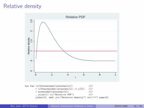
Relative density

.51

1.5

22.

50

Rel

ativ

e de

nsity

0 .2 .4 .6 .8 1r

Relative PDF

two fun (1/2*normalden(invnormal(x)) ///+ 1/2*normalden(invnormal(x),-1,1/2)) //// normalden(invnormal(x)) ///, yline(1) ti(”Relative PDF”) ///ylabel(0, add) yti(”Relative density”) xti(”r”) name(b)


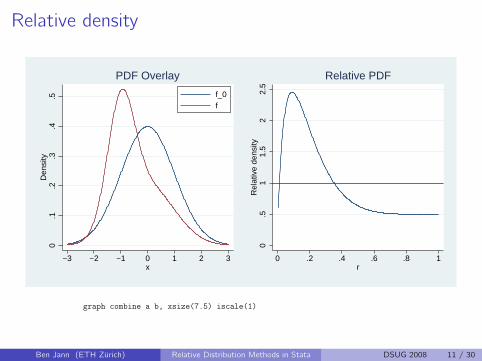
Relative density

0.1

.2.3

.4.5

Den

sity

−3 −2 −1 0 1 2 3x

f_0f

PDF Overlay

.51

1.5

22.

50

Rel

ativ

e de

nsity

0 .2 .4 .6 .8 1r

Relative PDF

graph combine a b, xsize(7.5) iscale(1)


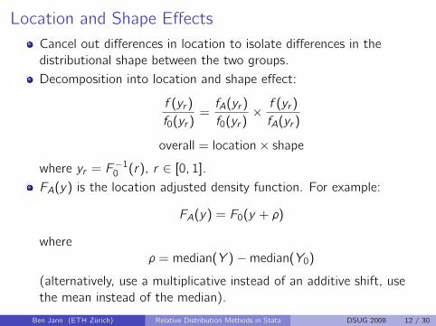
Location and Shape Effects

Cancel out differences in location to isolate differences in the

distributional shape between the two groups.

Decomposition into location and shape effect:

f (yr )

f0(yr )=fA(yr )

f0(yr )×f (yr )

fA(yr )

overall = location× shape

where yr = F−10 (r), r ∈ [0, 1].

FA(y) is the location adjusted density function. For example:

FA(y) = F0(y + ρ)

where

ρ = median(Y )−median(Y0)

(alternatively, use a multiplicative instead of an additive shift, use

the mean instead of the median).


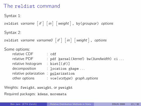
The reldist command

Syntax 1:

reldist varname[if

] [in

] [weight

], by(groupvar) options

Syntax 2:

reldist varname varname0[if

] [in

] [weight

], options

Some options:relative CDF : cdf

relative PDF : pdf kernel(kernel) bw(bandwidth) ci . . .

relative histogram : hist[(#)]

decomposition : location shape . . .

relative polarization : polarization

other options : vce(vcetype) graph options

Weights: fweight, aweight, or pweight

Required packages: kdens, moremata


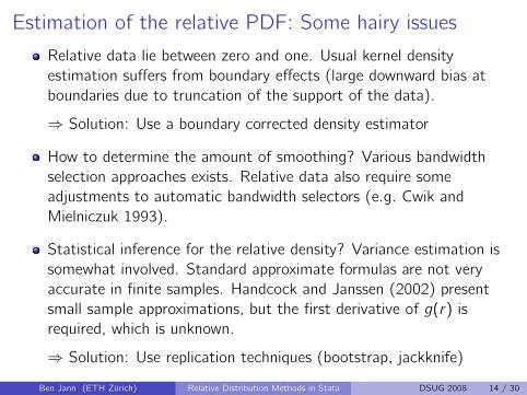
Estimation of the relative PDF: Some hairy issues

Relative data lie between zero and one. Usual kernel density

estimation suffers from boundary effects (large downward bias at

boundaries due to truncation of the support of the data).

⇒ Solution: Use a boundary corrected density estimator

How to determine the amount of smoothing? Various bandwidth

selection approaches exists. Relative data also require some

adjustments to automatic bandwidth selectors (e.g. Cwik and

Mielniczuk 1993).

Statistical inference for the relative density? Variance estimation is

somewhat involved. Standard approximate formulas are not very

accurate in finite samples. Handcock and Janssen (2002) present

small sample approximations, but the first derivative of g(r) isrequired, which is unknown.

⇒ Solution: Use replication techniques (bootstrap, jackknife)


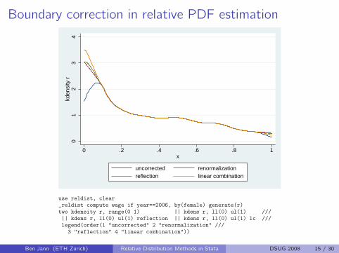
Boundary correction in relative PDF estimation

01

23

4kd

ensi

ty r

0 .2 .4 .6 .8 1x

uncorrected renormalizationreflection linear combination

use reldist, clear˙reldist compute wage if year==2006, by(female) generate(r)two kdensity r, range(0 1) —— kdens r, ll(0) ul(1) ///—— kdens r, ll(0) ul(1) reflection —— kdens r, ll(0) ul(1) lc ///legend(order(1 ”uncorrected” 2 ”renormalization” ///3 ”reflection” 4 ”linear combination”))


Examples

Data:

Swiss Labor Force Survey 1991 – 2006 (SLFS) by the Swiss Federal

Statistical Office

compare wages of men and women


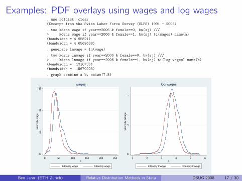
Examples: PDF overlays using wages and log wages. use reldist, clear(Excerpt from the Swiss Labor Force Survey (SLFS) 1991 - 2006)

. two kdens wage if year==2006 & female==0, bw(sj) ///¿ —— kdens wage if year==2006 & female==1, bw(sj) ti(wages) name(a)(bandwidth = 4.95821)(bandwidth = 4.6569638)

. generate lnwage = ln(wage)

. two kdens lnwage if year==2006 & female==0, bw(sj) ///¿ —— kdens lnwage if year==2006 & female==1, bw(sj) ti(log wages) name(b)(bandwidth = .1316736)(bandwidth = .15670923)

. graph combine a b, xsize(7.5)

0.0

1.0

2.0

3kd

ensi

ty w

age

0 50 100 150 200 250x

kdensity wage kdensity wage

wages

0.5

1kd

ensi

ty ln

wag

e

1 2 3 4 5 6x

kdensity lnwage kdensity lnwage

log wages


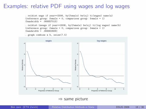
Examples: relative PDF using wages and log wages

. reldist wage if year==2006, by(female) bw(sj) ti(wages) name(a)(reference group: female = 0; comparison group: female = 1)(bandwidth = .066857015)

. reldist lnwage if year==2006, by(female) bw(sj) ti(log wages) name(b)(reference group: female = 0; comparison group: female = 1)(bandwidth = .066862669)

. graph combine a b, xsize(7.5)

1

2

3

4

0

Rel

ativ

e D

ensi

ty

0 .2 .4 .6 .8 1Proportion of Reference Group

wages

1

2

3

4

0

Rel

ativ

e D

ensi

ty


log wages

⇒ same picture


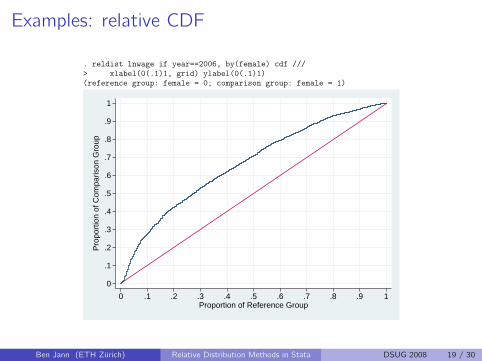
Examples: relative CDF

. reldist lnwage if year==2006, by(female) cdf ///¿ xlabel(0(.1)1, grid) ylabel(0(.1)1)(reference group: female = 0; comparison group: female = 1)

0

.1

.2

.3

.4

.5

.6

.7

.8

.9

1P

ropo

rtio

n of

Com

paris

on G

roup

0 .1 .2 .3 .4 .5 .6 .7 .8 .9 1Proportion of Reference Group


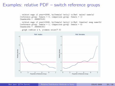
Examples: relative PDF – switch reference groups

. reldist wage if year==2006, by(female) bw(sj) ti(Ref: males) name(a)(reference group: female = 0; comparison group: female = 1)(bandwidth = .066857015)

. reldist wage if year==2006, by(female) bw(sj) ti(Ref: females) swap name(b)(reference group: female = 1; comparison group: female = 0)(bandwidth = .066956191)

. graph combine a b, ycommon xsize(7.5)

1

2

3

4

0

Rel

ativ

e D

ensi

ty


Ref: males

1

2

3

4

0

Rel

ativ

e D

ensi

ty


Ref: females


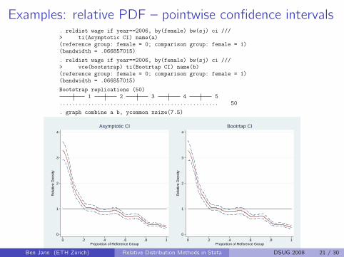
Examples: relative PDF – pointwise confidence intervals. reldist wage if year==2006, by(female) bw(sj) ci ///¿ ti(Asymptotic CI) name(a)(reference group: female = 0; comparison group: female = 1)(bandwidth = .066857015)

. reldist wage if year==2006, by(female) bw(sj) ci ///¿ vce(bootstrap) ti(Bootrtap CI) name(b)(reference group: female = 0; comparison group: female = 1)(bandwidth = .066857015)

Bootstrap replications (50)1 2 3 4 5

.................................................. 50

. graph combine a b, ycommon xsize(7.5)

1

2

3

4

0

Rel

ativ

e D

ensi

ty


Asymptotic CI

1

2

3

4

0

Rel

ativ

e D

ensi

ty


Bootrtap CI


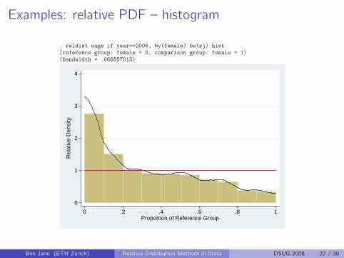
Examples: relative PDF – histogram

. reldist wage if year==2006, by(female) bw(sj) hist(reference group: female = 0; comparison group: female = 1)(bandwidth = .066857015)

1

2

3

4

0

Rel

ativ

e D

ensi

ty



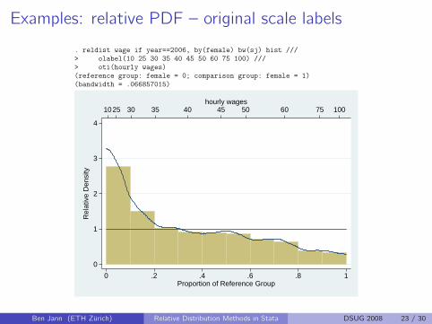
Examples: relative PDF – original scale labels

. reldist wage if year==2006, by(female) bw(sj) hist ///¿ olabel(10 25 30 35 40 45 50 60 75 100) ///¿ oti(hourly wages)(reference group: female = 0; comparison group: female = 1)(bandwidth = .066857015)

1

2

3

4

0

Rel

ativ

e D

ensi

ty

1025 30 35 40 45 50 60 75 100hourly wages



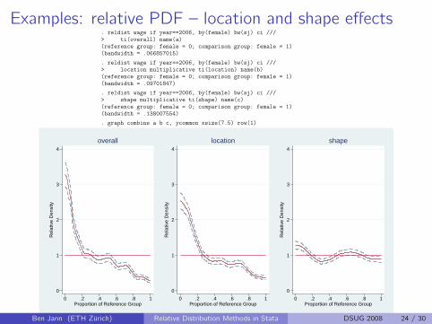
Examples: relative PDF – location and shape effects. reldist wage if year==2006, by(female) bw(sj) ci ///¿ ti(overall) name(a)(reference group: female = 0; comparison group: female = 1)(bandwidth = .066857015)

. reldist wage if year==2006, by(female) bw(sj) ci ///¿ location multiplicative ti(location) name(b)(reference group: female = 0; comparison group: female = 1)(bandwidth = .09701847)

. reldist wage if year==2006, by(female) bw(sj) ci ///¿ shape multiplicative ti(shape) name(c)(reference group: female = 0; comparison group: female = 1)(bandwidth = .138007554)

. graph combine a b c, ycommon xsize(7.5) row(1)

1

2

3

4

0

Rel

ativ

e D

ensi

ty


overall

1

2

3

4

0

Rel

ativ

e D

ensi

ty


location

1

2

3

4

0

Rel

ativ

e D

ensi

ty


shape


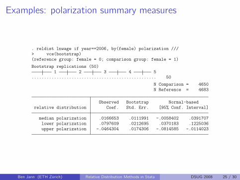
Examples: polarization summary measures

. reldist lnwage if year==2006, by(female) polarization ///¿ vce(bootstrap)(reference group: female = 0; comparison group: female = 1)

Bootstrap replications (50)1 2 3 4 5

.................................................. 50

N Comparison = 4650N Reference = 4683

Observed Bootstrap Normal-basedrelative distribution Coef. Std. Err. [95% Conf. Interval]

median polarization .0166653 .0111991 -.0058402 .0391707lower polarization .0797609 .0212695 .0370183 .1225036upper polarization -.0464304 .0174306 -.0814585 -.0114023


Conclusion

The relative distribution approach seems valuable for analyzing

distributional differences of a continuous outcome variable between

groups or time points.

A new user command called reldist provides these methods in

Stata (will be available from SSC in some time).

Some further issues:

Summary measures for the relative distribution. reldist supports

the MRP (median relative polarization). Other measures?

Accounting for the effects of covariates/decomposition of

distributional differences: How can this be done? (e.g. matching or

reweighting; problem: how to isolate the contributions of the

individual variables)


Thank you for your attention!


References I

Bernhardt, Annette, Martina Morris, and Mark S. Handcock (1995). Women’s

Gains or Men’s Losses? A Closer Look at the Shrinking Gender Gap in Earnings.

American Journal of Sociology 101(2): 302-328.

Blau, Francine D., and Lawrence M. Kahn (1992). The Gender Earnings Gap:

Learning from International Comparisons. American Economic Review 82(2):

533-538.

Blau, Francine D., and Lawrence M. Kahn (1996). International Differences in

Male Wage Inequality: Institutions versus Market Forces. Journal of Political

Economy 104(4): 791-837.

Blau, Francine D., and Lawrence M. Kahn (1996). Wage Structure and Gender

Earnings Differentials: an International Comparison. Economica 63(250):

S29-S62.

Blau, Francine D., and Lawrence M. Kahn (1997). Swimming Upstream: Trends

in the Gender Wage Differential in the 1980s. Journal of Labor Economics 15(1):

1-42.

Blinder, Alan S. (1973). Wage Discrimination: Reduced Form and Structural

Estimates. The Journal of Human Resources 8(4): 436-455.


References II

Buchinsky, Moshe (1998). The Dynamics of Changes in the Female Wage

Distribution in the USA: A Quantile Regression Approach. Journal of Applied

Econometrics 13(1): 1-30.

Cwik, Jan, and Jan Mielniczuk (1993). Data-dependent bandwidth choice for a

grade density kernel estimate. Statistics & Probability Letters 16: 397-405.

DiNardo, John E., Nicole Fortin, and Thomas Lemieux (1996). Labour Market

Institutions and the Distribution of Wages, 1973-1992: A Semiparametric

Approach. Econometrica 64(5): 1001-1046.

Handcock, Mark S., and Paul L. Janssen (2002). Statistical Inference for the

Relative Density. Sociological Methods and Research 30(3): 394-424.

Handcock, Mark S., and Martina Morris (1998). Relative Distribution Methods.

Sociological Methodology 28: 53-97.

Handcock, Mark S., and Martina Morris (1999). Relative Distribution Methods in

the Social Sciences. New York: Springer.

Juhn, Chinhui, Kevin M. Murphy, and Brooks Pierce (1991). Accounting for the

Slowdown in Black-White Wage Convergence. P. 107-143 in: Marvin Kosters

(ed.). Workers and Their Wages. Washington, DC: AEI Press.


References III

Juhn, Chinhui, Kevin M. Murphy, and Brooks Pierce (1993). Wage Inequality

and the Rise in Returns to Skill. Journal of Political Economy 101(3): 410-442.

Lemieux, Thomas (2002). Decomposing changes in wage distributions: a unified

approach. Canadian Journal of Economics 35(4): 646-688.

Machado, Jose A. F., and Jose Mata (2005). Counterfactual decomposition of

changes in wage distributions using quantile regression. Journal of Applied

Econometrics 20(4): 445-465.

Morris, Martina, Annette D. Bernhardt, and Mark S. Handcock (1994).

Economic Inequality: New Methods for New Trends. American Sociological

Review 59(2): 205-219.

Nopo, Hugo (2004). Matching as a Tool to Decompose Wage Gaps. IZA

Discussion Paper No. 981.

Oaxaca, Ronald (1973). Male-Female Wage Differentials in Urban Labor

Markets. International Economic Review 14(3): 693-709.


Documents

Relative Distribution Methods in Stata - Boston Collegefm · Outline Introduction The Relative Distribution Basic concepts Location and Shape Eﬀects Implementation: The reldist