ON IRREGULARITIES OF DISTRIBUTION RELATIVE TO … · DOI: 10.2478/udt-2018{0008 Unif. Distrib. Theory 13 (2018), no.2, 1{21 ON IRREGULARITIES OF DISTRIBUTION OF BINARY SEQUENCES RELATIVE

uniformdistribution

theory

DOI: 10.2478/udt-2018–0008

Unif. Distrib. Theory 13 (2018), no.2, 1–21

ON IRREGULARITIES OF DISTRIBUTION

OF BINARY SEQUENCES

RELATIVE TO ARITHMETIC PROGRESSIONS, II

(CONSTRUCTIVE BOUNDS)

Cecile Dartyge 1. — Katalin Gyarmati 2. — Andras Sarkozy 2.

1. Institut Elie Cartan, Universite de Lorraine, Nancy, Cedex, FRANCE

2. Eotvos Lorand University, Budapest, HUNGARY

ABSTRACT. In Part I of this paper we studied the irregularities of distributionof binary sequences relative to short arithmetic progressions. First we introduced

a quantitative measure for this property. Then we studied the typical and minimal

values of this measure for binary sequences of a given length. In this paper ourgoal is to give constructive bounds for these minimal values.

Communicated by Attila Petho

1. Introduction

First we recall some definitions and results from Part I of this paper [2].

K. F. R o t h [12] was the first who studied the irregularities of distributionof sequences relative to arithmetic progressions. It follows from his results that

Theorem 1 (R o t h [12]). If N,Q P N with Q ¤ N1{2 and EN � pe1, e2, . . .. . . , eN q P t�1,�1uN , then there are positive integers a, t, q such that

1 ¤ a ¤ a� pt� 1qq ¤ N, q ¤ Q

2010 M a t h e m a t i c s S u b j e c t C l a s s i f i c a t i o n: Primary 11K38, secondary 11B25.

K e y w o r d s: arithmetic progressions, irregularities of distribution, binary sequences.Research partially supported by Hungarian National Foundation for Scientific Research, GrantsNo. K100291, K119528 and NK104183 and the ANR-FWF bilateral project MuDeRa Multi-plicativity: Determinism and Randomness” (France-Austria).

1

CECILE DARTYGE—KATALIN GYARMATI—ANDRAS SARKOZY

and��t�1

j�0

ea�jq

�� ¡ c1Q1{2

with some absolute constant c1.

Binary sequences with strong pseudorandom properties play a crucial role incryptography and elsewhere. Thus in [7], M a u d u i t and S a r k o z y initiateda new constructive and quantitative approach to study pseudorandomness ofbinary sequences

EN � pe1, e2, . . . , eN q P t�1,�1uN . (1)

Among others, in [7] they introduced the following measures of pseudorandom-ness of binary sequences:

Definition 1. The well-distribution measure of the binary sequence (1) is de-fined by

W pEN q � maxa,b,t

��t�1

j�0

ea�jb

��where a, b, t P N and 1 ¤ a ¤ a� pt� 1qb ¤ N .

Definition 2. For k P N, k ¤ N the correlation measure of order k of thesequence (1) is defined as

CkpEN q � maxM,D

��M

n�1

en�d1en�d2 . . . en�dk

�� ,where M P N and D � pd1, . . . , dkq is a k-tuple of non-negative integers with0 ¤ d1 d2 � � � dk ¤ N �M .

Then the sequence EN P t�1,�1uN is said to possess strong pseudorandomproperties or, briefly, it is considered a “good” PR (= pseudorandom) sequenceif both W pEN q and CkpEN q (at least for “small” k) are small. There are manypapers written on these measures and constructions of “good” PR sequences, seePart I of this paper [2] for some related results and references.

We pointed out in Part I that in the applications one also needs binary se-quences of form (1) such that their “short” but “not too short” subsequences

EN pn,Mq � pen�1, en�2, . . . , en�M q (2)

(say of length M with N1�c M N for some c ¡ 0) also possess strong PR

properties. Thus our goal is to look for binary sequences of this type. First in thisseries we focus on the measure W (and we will study Ck, resp. the combinationof W and Ck later).

It follows from Theorem 1 and an upper bound estimate for

minENPt�1,�1uN

W pEN q

2

ON IRREGULARITIES OF DISTRIBUTION OF BINARY SEQUENCES, II

given by M a t o u s e k and S p e n c e r [6] that for all N P N we have

c2N1{4 min

ENPt�1,�1uNW pEN q c3N

1{4. (3)

Note that M a t o u s e k and S p e n c e r proved their upper bound by an exis-tence proof, and no constructive proof is known. Indeed, the best known con-struction (presented in [4] in 1978) gives only

W pEN q c4N1{3plogNq2{3. (4)

In Part I first we introduced a weighted version Wα of the measure W forstudying subsequences:

Definition 3. If EN is the binary sequence EN in (1) and 0 ¤ α ¤ 1{2, thenthe weighted α-well-distribution measure of EN is defined as

WαpEN q � max0¤n n�M¤N

M�αW�EN pn,Mq�.

We also needed the following modification of this measure:

Definition 4. If EN is the binary sequence EN in (1) and 0 ¤ α ¤ 1{2, thenthe modified α-well-distribution measure of EN is defined as

WαpEN q � max0 M N

�M�α max

1¤a¤a�pM�1qb¤N

��M�1¸j�0

ea�jb

��.

Next we showed that for a truly random EN P t�1,�1uN the Wα measure ofit is around N1{2�α (we present this result here in a slightly simplified but lesssharp form):

Theorem 2. Assume that 0 ¤ α ¤ 1{2. Then for all ε ¡ 0 there are numbersN0 � N0pεq and δ � δpεq such that if N ¡ N0, then for a truly random sequenceEN � t�1,�1uN (i.e., choosing each EN P t�1,�1uN with probability 1{2N )we have

P�δN1{2�α WαpEN q 6N1{2�αplogNq1{2

¡ 1� ε.

WritemαpNq � min

ENPt�1,�1uNWαpEN q and mαpNq � min

ENPt�1,�1uNWαpEN q.

A trivial lower bound for mαpNq is

mαpNq " N1{4�α for all 0 ¤ α ¤ 1{2. (5)

We conjectured that much more is true:

Conjecture 1. For 0 ¤ α ¤ 1{2 we have

c5N1{4�α{2 mαpNq c6N

1{4�α{2. (6)

3


Note that by (3) this is true for α � 0. For α ¡ 0 we have not been able toimprove on (5). Thus instead we proved two theorems which can be consideredas partial results towards the lower bound part of this conjecture: first we gavea lower bound for mαpNq, and then we proved a lower bound for WαpEN q fromwhich it follows that for almost all EN P t�1,�1uN the Wα measure of EN isgreater than the lower bound in (6) divided by a logarithm factor:

WαpEN q " N1{4�α{2

plogNq1{4�α{2 .

In this paper our goal is to study certain special sequences EN with smallvalues of WαpEN q. First in Section 2 we will show that the Rudin-Shapirosequence possesses small Wα measure for all α. Then in Sections 3 and 4 we willgive upper bounds for small values of Wα in case of Legendre symbol sequences.Finally, in Section 5 we will give lower bound for Wα for the Legendre symbolconstruction.

2. Upper bound for small values of Wα

uniformly in α for the Rudin-Shapiro sequence

Unfortunately, we have not been able to prove that the upper bound in (3)can be extended to the case of general α as presented in Conjecture 1; namely,we have not been able to extend the existence proof given by M a t o u s e k andS p e n c e r in [6]. On the other hand, we will be able to extend and sharpen theconstructive upper bound (4) in various directions by giving constructive proofs.First in this section we will give a partial answer to the questions asked at theend of Section 1 in [2]: we will show that the truncated Rudin-Shapiro sequenceis well-distributed in short blocks of consecutive elements of it, in other words,Wα is small uniformly in α for this sequence.

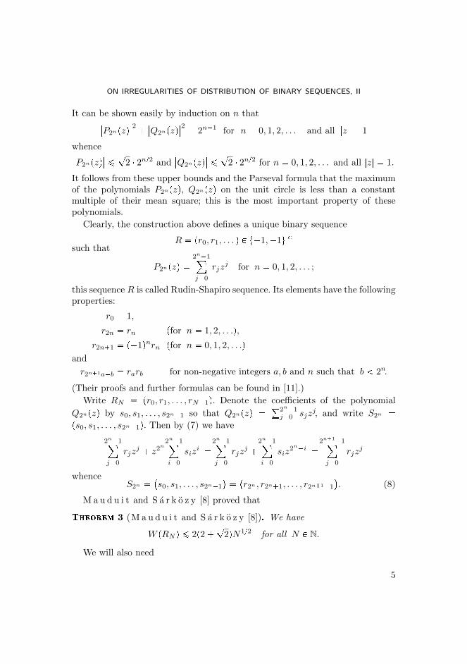
The Rudin-Shapiro sequence [13], [15] plays a role of basic importance in har-monic analysis. Its definition is the following:

First we define pairs of polynomials P2npzq, Q2npzq pn � 0, 1, 2, . . . q of degree2n � 1 by the following recursion: Let

P1pzq � Q1pzq � 1,

and if P2npzq and Q2npzq have been defined for a non-negative integer n, then let

P2n�1pzq � P2npzq � z2nQ2npzq and Q2n�1pzq � P2npzq � z2nQ2npzq. (7)

4


It can be shown easily by induction on n that��P2npzq��2 � ��Q2npzq

��2 � 2n�1 for n � 0, 1, 2, . . . and all |z| � 1

whence��P2npzq�� ¤ ?

2 � 2n{2 and��Q2npzq

�� ¤ ?2 � 2n{2 for n � 0, 1, 2, . . . and all |z| � 1.

It follows from these upper bounds and the Parseval formula that the maximumof the polynomials P2npzq, Q2npzq on the unit circle is less than a constantmultiple of their mean square; this is the most important property of thesepolynomials.

Clearly, the construction above defines a unique binary sequence

R � pr0, r1, . . . q P t�1,�1u8such that

P2npzq �2n�1¸j�0

rjzj for n � 0, 1, 2, . . . ;

this sequence R is called Rudin-Shapiro sequence. Its elements have the followingproperties:

r0 � 1,

r2n � rn pfor n � 1, 2, . . .q,r2n�1 � p�1qnrn pfor n � 0, 1, 2, . . .q

and

r2n�1a�b � rarb for non-negative integers a, b and n such that b 2n.

(Their proofs and further formulas can be found in [11].)

Write RN � pr0, r1, . . . , rN�1q. Denote the coefficients of the polynomial

Q2npzq by s0, s1, . . . , s2n�1 so that Q2npzq �°2n�1j�0 sjz

j, and write S2n �ps0, s1, . . . , s2n�1q. Then by (7) we have

2n�1¸j�0

rjzj � z2n

2n�1¸i�0

sizi �

2n�1¸j�0

rjzj �

2n�1¸i�0

siz2n�i �

2n�1�1¸j�0

rjzj

whenceS2n �

�s0, s1, . . . , s2n�1

� � �r2n , r2n�1, . . . , r2n�1�1

�. (8)

M a u d u i t and S a r k o z y [8] proved that

Theorem 3 (M a u d u i t and S a r k o z y [8]). We have

W pRN q ¤ 2p2�?

2qN1{2 for all N P N.

We will also need

5


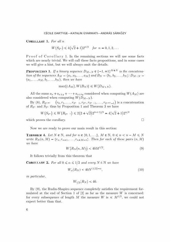
Corollary 1. For all n

W pS2nq ¤ 4�?

2� 1�2n{2 for n � 0, 1, 2, . . .

P r o o f o f C o r o l l a r y 1. In the remaining sections we will use some factswhich are nearly trivial. We will call these facts propositions, and in some caseswe will give a hint, but we will always omit the details.

Proposition 1. If a binary sequence DM�N P t�1,�1uM�N is the concatena-tion of the sequences AM � pa1, a2, . . . , aM q and BN � pb1, b2, . . . , bN q: DM�N �pa1, . . . , aM , b1, . . . , bN q, then we have

max�pAM q,W pBN q

� ¤W pDM�N q.

All the sums ax�ax�y�� ax�ty considered when computing W pAM q arealso considered when computing W pDM�N q.

By (8), R2n�1 � �r0, r1, . . . , r2n�1, r2n , r2n�1, . . . , r2n�1�1

�is a concatenation

of R2n and S2n thus by Proposition 1 and Theorem 3 we have

W�S2n

� ¤W�R2n�1

� ¤ 2�2�

?2�2pn�1q{2 � 4

�?2� 1

�2n{2

which proves the corollary. �

Now we are ready to prove our main result in this section:

Theorem 4. Let N P N, and for n P t0, 1, . . . u, M P N, 0 ¤ n n �M ¤ Nwrite RN pn,Mq � prn, rn�1, . . . , rn�M�1q. Then for each of these pairs pn,Mqwe have

W�RN pn,Mq� 40M1{2. (9)

It follows trivially from this theorem that

Corollary 2. For all 0 ¤ α ¤ 1{2 and every N P N we have

WαpRN q 40N p1{2q�α, (10)

in particular,

W1{2pRN q 40.

By (9), the Rudin-Shapiro sequence completely satisfies the requirement for-mulated at the end of Section 1 of [2] as far as the measure W is concerned:for every subsequence of length M the measure W is ! M1{2, we could notexpect better than that.

6


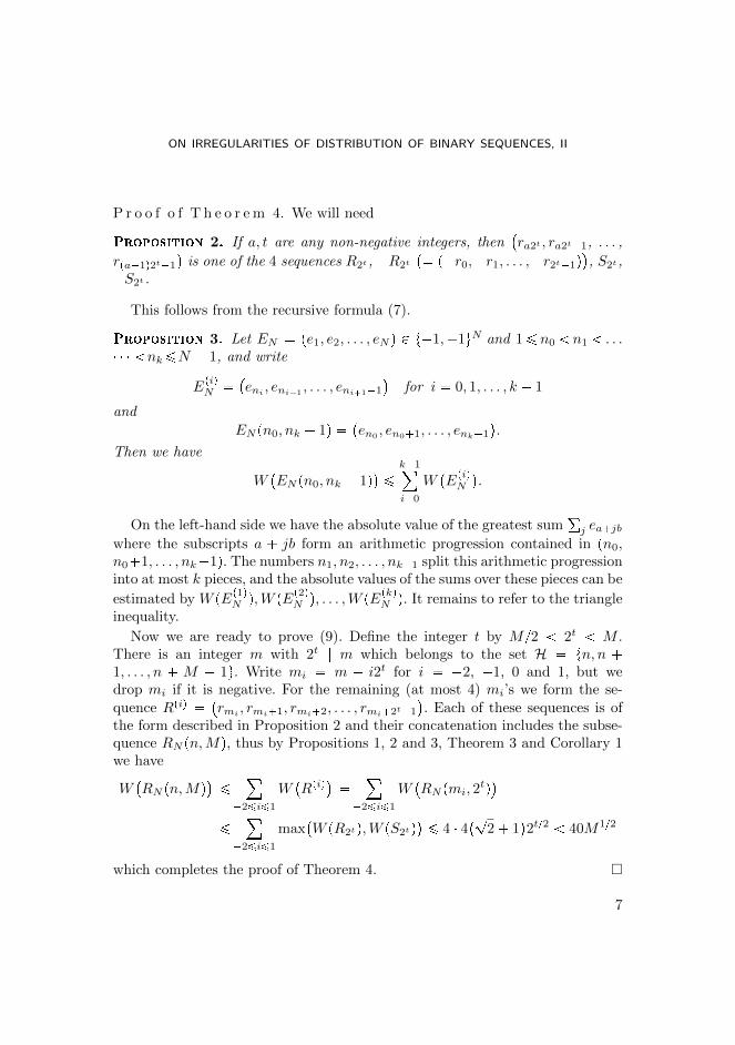
P r o o f o f T h e o r e m 4. We will need

Proposition 2. If a, t are any non-negative integers, then�ra2t , ra2t�1, . . . ,

rpa�1q2t�1

�is one of the 4 sequences R2t , �R2t

�� p�r0,�r1, . . . ,�r2t�1q�, S2t ,

�S2t .

This follows from the recursive formula (7).

Proposition 3. Let EN � pe1, e2, . . . , eN q P t�1,�1uN and 1¤ n0 n1 . . .� � � nk¤N � 1, and write

EpiqN � �

eni , eni�1, . . . , eni�1�1

�for i � 0, 1, . . . , k � 1

and

EN pn0, nk � 1q � �en0

, en0�1, . . . , enk�1

�.

Then we have

W�EN pn0, nk � 1q� ¤ k�1

i�0

W�EpiqN

�.

On the left-hand side we have the absolute value of the greatest sum°j ea�jb

where the subscripts a � jb form an arithmetic progression contained in pn0,n0�1, . . . , nk�1q. The numbers n1, n2, . . . , nk�1 split this arithmetic progressioninto at most k pieces, and the absolute values of the sums over these pieces can be

estimated by W pEp1qN q,W pEp2q

N q, . . . ,W pEpkqN q. It remains to refer to the triangle

inequality.

Now we are ready to prove (9). Define the integer t by M{2 2t M .There is an integer m with 2t | m which belongs to the set H � tn, n �1, . . . , n � M � 1u. Write mi � m � i2t for i � �2, �1, 0 and 1, but wedrop mi if it is negative. For the remaining (at most 4) mi’s we form the se-quence Rpiq � �

rmi , rmi�1, rmi�2, . . . , rmi�2t�1

�. Each of these sequences is of

the form described in Proposition 2 and their concatenation includes the subse-quence RN pn,Mq, thus by Propositions 1, 2 and 3, Theorem 3 and Corollary 1we have

W�RN pn,Mq� ¤ ¸

�2¤i¤1

W�Rpiq

� � ¸�2¤i¤1

W�RN pmi, 2

tq�¤

¸�2¤i¤1

max�W pR2tq,W pS2tq

� ¤ 4 � 4�?2� 1�2t{2 40M1{2

which completes the proof of Theorem 4. �

7


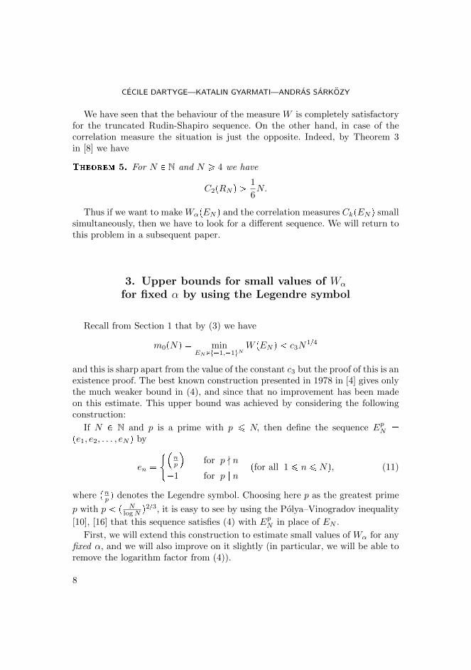
We have seen that the behaviour of the measure W is completely satisfactoryfor the truncated Rudin-Shapiro sequence. On the other hand, in case of thecorrelation measure the situation is just the opposite. Indeed, by Theorem 3in [8] we have

Theorem 5. For N P N and N ¥ 4 we have

C2pRN q ¡ 1

6N.

Thus if we want to make WαpEN q and the correlation measures CkpEN q smallsimultaneously, then we have to look for a different sequence. We will return tothis problem in a subsequent paper.

3. Upper bounds for small values of Wα

for fixed α by using the Legendre symbol

Recall from Section 1 that by (3) we have

m0pNq � minENPt�1,�1uN

W pEN q c3N1{4

and this is sharp apart from the value of the constant c3 but the proof of this is anexistence proof. The best known construction presented in 1978 in [4] gives onlythe much weaker bound in (4), and since that no improvement has been madeon this estimate. This upper bound was achieved by considering the followingconstruction:

If N P N and p is a prime with p ¤ N, then define the sequence EpN �pe1, e2, . . . , eN q by

en �#�

np

for p - n

�1 for p | npfor all 1 ¤ n ¤ Nq, (11)

where pnp q denotes the Legendre symbol. Choosing here p as the greatest prime

p with p p NlogN q2{3, it is easy to see by using the Polya–Vinogradov inequality

[10], [16] that this sequence satisfies (4) with EpN in place of EN .

First, we will extend this construction to estimate small values of Wα for anyfixed α, and we will also improve on it slightly (in particular, we will be able toremove the logarithm factor from (4)).

8


Theorem 6. For every α with 0 ¤ α ¤ 1{2 there is a number N0 � N0pαq suchthat if N P N, N ¡ N0 then there is a prime p with

1

2N

2p1�αq3 p ¤ N

2p1�αq3 (12)

so that for the sequence EpN defined by (11) we have

WαpEpN q c5N1�α3 (13)

where c5 is an absolute constant (independent of α).

Compare this upper bound with the upper bound for WαpRN q in (10): in (10)the exponent of N is 1

2�α while here in (13) the exponent is 1�α3 which is smaller

than 12 � α for 0 ¤ α 1{4.

In the special case α � 0 we get from Theorem 6 that

Corollary 3. For N P N, N ¡ N0 there is a prime p with

1

2N2{3 p ¤ N2{3

such that for the sequence EpN we have

W pEpN q �W0pEpN q c5N1{3.

(Indeed, this is better than (4) by a factor plogNq2{3.)

P r o o f o f T h e o r e m 6. The proof will be based on a result of M o n t g o -m e r y and V a u g h a n [9]:

Lemma 1. There is an absolute constant c6 such that for N P N, N ¥ 2 thereis a prime p satisfying

N

2 p ¤ N

and ��X�Y

n�X�1

�n

p

�� c6p1{2 for all X P Z, Y P N. (14)

(Here and in the rest of this paper we define pnp q � 0 for p | n.)

P r o o f o f L e m m a 1. This follows from (ii) in the Corollary in [9] by takingany θ ¡ 1{2 there (and using also the prime number theorem). �

For Y P N write

dpp, Y q � maxXPZ

��X�Y

n�X�1

�n

p

�� . (15)

9


We will also need

Lemma 2. If M,N P N, n P t0, 1, . . . , N � 1u, n �M ¤ N and p is a primewith p ¤ N , then we have

W�EpN pn,Mq� ¤ max

Y¤Mdpp, Y q � 2M

p� 2. (16)

P r o o f o f L e m m a 2. By the definitions of W pEN q, EpN � pe1, e2, . . . , eN qand EN pn,Mq we have

W�EpN pn,Mq� � max

a,b,t

��t�1

j�0

ea�jb

��

� maxa,b,t

��t�1

j�0

�a� jb

p

�

¸0¤j tp|a�jb

1

��, (17)

where a, b, t P N and

n� 1 ¤ a ¤ a� pt� 1qb ¤ n�M. (18)

It follows from (18) that

pt� 1qb � pa� pt� 1qbq � a ¤ pn�Mq � pn� 1q �M � 1 (19)

whence

t ¤ M � 1

b� 1 M

b� 1 ¤M � 1

so thatt ¤M. (20)

If pb, pq � 1, then by the definition of dpp, Y q and (20) we have��t�1

j�0

�a� jb

p

�

¸0¤j tp|a�jb

1

��¤

��t�1

j�0

�a� jb

p

��¸

0¤j tp|a�jb

1

��t�1

j�0

�ab�1 � j

p

�� |tj : jb � �a pmod pq, 0 ¤ j tu|

¤ dpp, tq ��t

p� 1

¤ max

t¤Mdpp, tq � M

p� 1 pfor pb, pq � 1q. (21)

10


If pb, pq ¡ 1, then we have b ¥ p thus it follows from (19) that

pt� 1qp ¤ pt� 1qb ¤M � 1

whence

t ¤ M � 1

p� 1 M

p� 1.

Thus we have��t�1

j�0

�a� jb

p

�

¸0¤j tp|a�jb

1

��¤ 2

t�1

j�0

1 � 2t 2M

p� 2 pfor pb, pq ¡ 1q. (22)

(16) follows from (17), (21) and (22) which completes the proof of the lemma. �

In order to prove the statement of the theorem we use Lemma 1 with N2p1�αq

3

in place of N. We get for N large enough that there is a prime p satisfying (12)such that (14) holds. Then by the definition of Wα, (12), (14), (15) and Lemma 2we have

WαpEpN q � max0¤n n�M¤N

M�αW�EpN pn,Mq�

¤ max0¤n n�M¤N

M�α

�maxY¤M

dpp, Y q � 2M

p� 2

¤ maxM¤N

M�α

�c6p

1{2 � 2M

p� 2

maxM¤N

c7

�p1{2 � M1�α

p

¤ c7

�p1{2 � N1�α

p

c8N

1�α3 (23)

which completes the proof of Theorem 6. �

For 0 α p¤ 1{2q one can improve further on the upper bound in (13)by using the Burgess inequality:

Theorem 7. For every α with 0 ¤ α ¤ 1{2 there is a number N1 � N1pαqsuch that if N P N, N ¡ N1 and p is a prime which satisfies the inequalities

in Lemma 1 with N8p1�αq12�5α plogNq� 8α

12�5α in place of N :

1

2N

8p1�αq12�5α plogNq� 8α

12�5α p ¤ N8p1�αq12�5α plogNq� 8α

12�5α (24)

and (14) holds, then we have

WαpEpN q c9Np1�αqp4�5αq

12�5α plogNq 8α12�5α , (25)

where c9 is an absolute constant (independent of α).

11


Observe that the exponent p1�αqp4�5αq12�5α in the upper bound in (25) is smaller

than the exponent 1�α3 in (13) in Theorem 6 for all 0 α (in particular,

for α � 1{2 these exponents are 338 and 1

6 , respectively).

P r o o f o f T h e o r e m 7. By the Burgess inequality [1] we have

Lemma 3. If p is a prime number and H P N, r P N, then

dpp,Hq � maxXPZ

��X�H

n�X�1

�n

p

�� c10H1� 1

r pr�1

4r2 plog pq1{r,

where c10 is an absolute constant.

(Here c10 � 30 can be taken [18].)

In order to estimate WαpEpN q in the theorem again we use Lemma 2:



¤ maxM¤N

M�α

�maxH¤M

dpp,Hq � 2M

p� 2

¤ maxM¤N

�M�α max

H®Mdpp,Hq � 2

M1�α

p� 2M�α

¤ maxM¤N

�M�α max

H¤Mdpp,Hq

� 4

N1�α

p(26)

since we have p N1�α by the upper bound for p in (24) and α ¤ 1{2. By α ¥ 0here we have

maxM¤N

�M�α max

H¤Mdpp,Hq

¤ maxH¤N

dpp,Hq maxH¤M¤N

M�α

� maxH¤N

H�αdpp,Hq � maxH¤N

F pHq, (27)

where F pHq � H�αdpp,Hq.It remains to estimate F pHq for H P p0, N s. To do this, we split the in-

terval p0, N s into subintervals. To define these subintervals we introduce thefollowing notations:

Let R be a positive integer large enough in terms of α which will be fixedlater. Let t1 � N , t2 � p5{8plog pq�1,

tr � pr2�r�14pr�1qr log p for r � 3, 4, . . . , R� 1

and tR�2 � 0 (where p is the prime p defined in the theorem). A simple compu-tation shows that if N is large enough (in terms of α), then we have

0 � tR�2 tR�1 � � � t2 t1 � N. (28)

12


Let Ir � ptr�1, trs for r � 1, 2, . . . , R � 1. Then it follows from (28) that theinterval p0, N s is a disjoint union of the intervals Ir:

p0, N s �R�1¤r�1

Ir, Ir X Ir1 � H for 1 ¤ r r1 ¤ R� 1. (29)

First for H P I1 we estimate F pHq by (14):

F pHq � H�αdpp,Hq t�α2 c6p1{2 � c6p

�5α{8plog pqαp1{2

� c6p1{2�5α{8plog pqα � c6Gp1q � c6p

u1plog pqv1 pfor H P I1q (30)

with Gp1q � pu1plog pqv1, u1 � 1{2� 5α{8, v1 � α.

For H belonging to the r-th interval Ir � ptr�1, trs with 1 r R�1 we usethe Burgess inequality in Lemma 3 with this r (indeed, Ir is defined so that thisr value should give the optimal bound):

F pHq � H�αdpp,Hq c10H�αH1� 1

r pr�1

4r2 plog pq1{r

� c10H1�α� 1

r pr�1

4r2 plog pq1{r.

By α ¤ 1{2 the exponent of H is non-negative, thus we get

F pHq c10t1�α� 1

rr p

r�1

4r2 plog pq1{rwhence for r � 2 we have

F pHq c10t1{2�α2 p3{16plog pq1{2

� c10p5{16�5α{8plog pqα�1{2p3{16plog pq1{2

� c10p1{2�5α{8plog pqα

� c10Gp2q � c10pu2plog pqv2 pfor H P I2q (31)

with Gp2q � pu2plog pqv2, u2 � 12 � 5α

8 and v2 � α, while for 2 r R � 1we get

F pHq c10

�pr2�r�14pr�1qr log p

1�α� 1r

pr�1

4r2 plog pq 1r

� c10pr�24r �α r

2�r�14pr�1qr plog pq1�α � c10Gprq

� c10pur plog pqvr pfor H P Ir, 2 R R� 1q (32)

with Gprq � pur plog pqvr, ur � r�24r � α r

2�r�14pr�1qr and vr � 1� α.

13


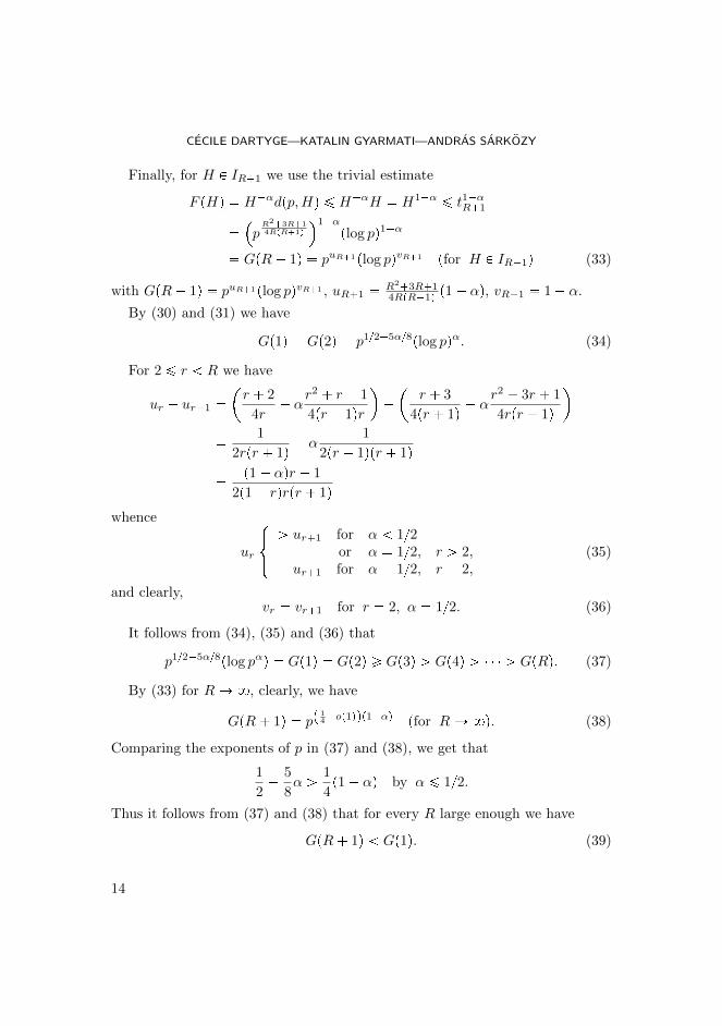
Finally, for H P IR�1 we use the trivial estimate

F pHq � H�αdpp,Hq ¤ H�αH � H1�α ¤ t1�αR�1

��pR2�3R�14RpR�1q

1�α

plog pq1�α

� GpR� 1q � puR�1plog pqvR�1 pfor H P IR�1q (33)

with GpR� 1q � puR�1plog pqvR�1 , uR�1 � R2�3R�14RpR�1q p1� αq, vR�1 � 1� α.

By (30) and (31) we have

Gp1q � Gp2q � p1{2�5α{8plog pqα. (34)

For 2 ¤ r R we have

ur � ur�1 ��r � 2

4r� α

r2 � r � 1

4pr � 1qr��

r � 3

4pr � 1q � αr2 � 3r � 1

4rpr � 1q

� 1

2rpr � 1q � α1

2pr � 1qpr � 1q� p1� αqr � 1

2p1� rqrpr � 1qwhence

ur

$&%

¡ ur�1 for α 1{2or α � 1{2, r ¡ 2,

� ur�1 for α � 1{2, r � 2,(35)

and clearly,vr � vr�1 for r � 2, α � 1{2. (36)

It follows from (34), (35) and (36) that

p1{2�5α{8plog pαq � Gp1q � Gp2q ¥ Gp3q ¡ Gp4q ¡ � � � ¡ GpRq. (37)

By (33) for RÑ8, clearly, we have

GpR� 1q � pp 14�op1qqp1�αq pfor RÑ8q. (38)

Comparing the exponents of p in (37) and (38), we get that

1

2� 5

8α ¡ 1

4p1� αq by α ¤ 1{2.

Thus it follows from (37) and (38) that for every R large enough we have

GpR� 1q Gp1q. (39)

14


Now we fix the value of R: let R be the smallest integer R with R ¡ 2 for which(39) holds. Then it follows from (26), (27), (29), (30), (31), (32), (33), (37) and(39) that

WαpEpN q c11p1{2�5α{8plog pqα � 4

N1�α

p(40)

whence (25) follows using that the prime p satisfies (24) (note that this choice of pbalances the two terms in (40)) and this completes the proof of Theorem 7. �

4. Conditional upper boundfor the Legendre symbol construction

In Section 3 we estimated WαpEpN q for the Legendre symbol sequence EpNin (11) by using the best known estimates for Legendre symbol sums. However,these estimates are probably very far from being sharp so that WαpEpN q is muchsmaller than our upper bounds. Thus it seems worth to study what upper boundcan be given for WαpEpN q having a plausible hypothesis on the size of Legendresymbol sums? Such a hypothesis was formulated, e.g., by L. Z h a o in [18]: If χis a non-principal character modulo a prime number p and we set

SχpNq �¸

M n¤M�N

χpnq,

then “the expected bound is

SχpNq !?N pε.” (41)

We will call (41) hypothesis H, and we will estimate WαpEpN q under this hy-pothesis.

Theorem 8. Assume that hypothesis H holds with χpnq ��np

, i.e., for every

ε ¡ 0 there is a number p0 � p0pεq such that for every prime p ¡ p0 we have

dpp, Y q � maxXPZ

��X�Y

n�X�1

�n

p

�� ! Y 1{2pε pfor all p ¡ p0 and Y P Nq. (42)

Then for every α and ε with 0 ¤ α ¤ 1{2 and ε ¡ 0 there is a number N0 �N0pα, εq such that if N P N, N ¡ N0, then there is a prime p with

1

2N

2�2α3�2α p ¤ N

2�2α3�2α

�¤ N1�α�

(43)

so that for the sequence EpN defined by (11) we have

WαpEpN q Np1�αqp1�2αq

3�2α �ε. (44)

15


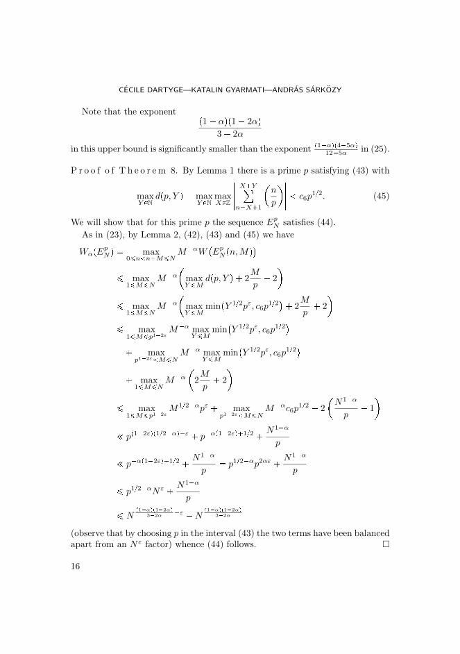
Note that the exponentp1� αqp1� 2αq

3� 2α

in this upper bound is significantly smaller than the exponent p1�αqp4�5αq12�5α in (25).

P r o o f o f T h e o r e m 8. By Lemma 1 there is a prime p satisfying (43) with

maxY PN

dpp, Y q � maxY PN

maxXPZ

��X�Y

n�X�1

�n

p

�� c6p1{2. (45)

We will show that for this prime p the sequence EpN satisfies (44).

As in (23), by Lemma 2, (42), (43) and (45) we have



¤ max1¤M¤N

M�α

�maxY¤M

dpp, Y q � 2M

p� 2

¤ max1¤M¤N

M�α

�maxY¤M

min�Y 1{2pε, c6p

1{2�� 2

M

p� 2

¤ max1¤M¤p1�2ε

M�α maxY¤M

min�Y 1{2pε, c6p

1{2�

� maxp1�2ε M¤N

M�α maxY¤M

min�Y 1{2pε, c6p

1{2�

� max1¤M¤N

M�α

�2M

p� 2

¤ max1¤M¤p1�2ε

M1{2�αpε � maxp1�2ε M¤N

M�αc6p1{2 � 2

�N1�α

p� 1

! pp1�2εqp1{2�αq�ε � p�αp1�2εq�1{2 � N1�α

p

! p�αp1�2εq�1{2 � N1�α

p� p1{2�αp2αε � N1�α

p

¤ p1{2�αNε � N1�α

p

¤ Np1�αqp1�2αq

3�2α �ε �Np1�αqp1�2αq

3�2α

(observe that by choosing p in the interval (43) the two terms have been balancedapart from an Nε factor) whence (44) follows. �

16


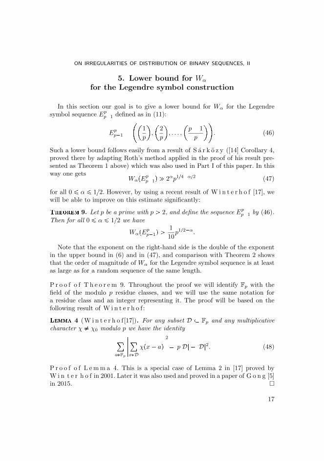
5. Lower bound for Wα

for the Legendre symbol construction

In this section our goal is to give a lower bound for Wα for the Legendresymbol sequence Epp�1 defined as in (11):

Epp�1 ��

1

p

,

�2

p

, . . . ,

�p� 1

p

�. (46)

Such a lower bound follows easily from a result of S a r k o z y ([14] Corollary 4,proved there by adapting Roth’s method applied in the proof of his result pre-sented as Theorem 1 above) which was also used in Part I of this paper. In thisway one gets

WαpEpp�1q " 2αp1{4�α{2 (47)

for all 0 ¤ α ¤ 1{2. However, by using a recent result of W i n t e r h o f [17], wewill be able to improve on this estimate significantly:

Theorem 9. Let p be a prime with p ¡ 2, and define the sequence Epp�1 by (46).

Then for all 0 ¤ α ¤ 1{2 we have

WαpEpp�1q ¡1

10p1{2�α.

Note that the exponent on the right-hand side is the double of the exponentin the upper bound in (6) and in (47), and comparison with Theorem 2 showsthat the order of magnitude of Wα for the Legendre symbol sequence is at leastas large as for a random sequence of the same length.

P r o o f o f T h e o r e m 9. Throughout the proof we will identify Fp with thefield of the modulo p residue classes, and we will use the same notation fora residue class and an integer representing it. The proof will be based on thefollowing result of W i n t e r h o f:

Lemma 4 (W i n t e r h o f[17]). For any subset D � Fp and any multiplicativecharacter χ � χ0 modulo p we have the identity

¸aPFp

��¸xPD

χpx� aq��2

� p|D| � |D|2. (48)

P r o o f o f L e m m a 4. This is a special case of Lemma 2 in [17] proved byW i n t e r h o f in 2001. Later it was also used and proved in a paper of G o n g [5]in 2015. �

17


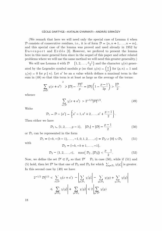
(We remark that here we will need only the special case of Lemma 4 whenD consists of consecutive residues, i.e., it is of form D � tn, n � 1, . . . , n �mu,and this special case of the lemma was proved and used already in 1952 byD a v e n p o r t and E r d o s [3]. However, we prefered to present the lemmahere in this more general form since in the sequel of this paper and other relatedproblems where we will use the same method we will need this greater generality.)

We will use Lemma 4 with D � 1, 2, . . . , p�1

2

(and the character χpnq gener-

ated by the Legendre symbol modulo p (so that χpnq ��np

for pp, nq � 1 and

χpnq � 0 for p | n). Let a1 be an a value which defines a maximal term in thesum in (48) so that this term is at least as large as the average of the terms:��

¸xPD

χpx� a1q��2

¥ |D| � |D|2p

� |D|�

1� p� 1

2p

¡ |D|

2

whence ��¸xPD

χpx� a1q�� ¡ 2�1{2|D|1{2. (49)

Write

D1 � D � ta1u �"a1 � 1, a1 � 2, . . . , a1 � p� 1

2

*.

Then either we have

D1 � t1, 2, . . . , p� 1u, |D1| � |D| � p� 1

2(50)

or D1 can be represented in the form

D1 � t�b,�pb� 1q, . . . ,�1, 0, 1, 2, . . . , cu � D2 Y t0u YD3 (51)

withD2 � t�b,�b� 1, . . . ,�1u,

D3 � t1, 2, . . . , cu, max�|D2|, |D3|

� p� 1

2. (52)

Now, we define the set D1 � Fp so that D1 � D1 in case (50), while if (51) and

(5) hold, then let D1 be that one of D2 and D3 for which��°yPDi χpyq

�� is greater.

In this second case by (49) we have

2�1{2|D|1{2 ��¸xPD

χpx� a1q��

��¸yPD1

χpyq��

��¸yPD2

χpyq �¸yPD3

χpyq��

¤��¸yPD2

χpyq��

��¸yPD3

χpyq�� ¤ 2

��¸yPD1

χpyq��

18


whence��¸yPD1

χpyq�� ¡ 2�3{2|D|1{2. (53)

In the first case (50), we have��¸yPD1

χpyq��

��¸yPD1

χpyq��

��¸xPD

χpx� a1q��

from which again (53) follows by (49).

It follows from the definition of D1 that in both cases it is of the form

D1 � tn� 1, n� 2, . . . , n�Mu (54)with

1 ¤ n� 1 n�M ¤ p� 1 (55)

and, by also using (50) and (5), we have

M � |D1| ¤ p� 1

2. (56)

We obtain from (53), (54), (55) and (56) that

W pEpp�1q ¥M�αW�Epp�1pn,Mq�

¥M�α��en�1 � en�2 � � � � � en�M

��M�α

��¸yPD1

χpyq�� M�α

��M

i�1

�n� i

p

��¡ |D1|�α2�3{2|D|1{2

¥ |D|�α2�3{2|D|1{2 � 2�3{2|D|1{2�α

� 2�3{2

�p� 1

2

1{2�α

¥ 2�3{2�p

4

1{2�α

� 2�3{2p2�2q1{2�αp1{2�α

¥ 2�5{2p1{2�α

¡ 1

10p1{2�α

which completes the proof of the theorem. �

19


REFERENCES

[1] BURGESS, D. A.: On character sums and primitive roots, Proc. London Math. Soc. 12(1962), no. 3, 179–192.

[2] DARTYGE, C.—GYARMATI, K.—SARKOZY, A.: On irregularities of distribution of bi-

nary sequences relative to arithmetic progressions, I. (General results), Unif. Distrib.

Theory 12 (2017), no. 1, 55–67.

[3] DAVENPORT, H.—ERDOS, P.: The distribution of quadratic and higher residues, Publ.

Math. Debrecen 2 (1952), 252-265.

[4] ERDOS, P.—SARKOZY, A.: Some solved and unsolved problems in combinatorial num-ber theory, Math. Slovaca 28 (1978), 407–421.

[5] GONG, K.: An elementary approach to character sums over multiplicative subgroups,Integers 16 (2016), #A13.

[6] MATOUSEK, J.—SPENCER, J.: Discrepancy in arithmetic progression, J. Amer. Math.

Soc. 9 (1996), 195–204.

[7] MAUDUIT, C.—SARKOZY, A.: On finite pseudorandom binary sequences, I. Measureof pseudorandomness, the Legendre symbol, Acta Arith. 82 (1997), 365–377.

[8] MAUDUIT, C.—SARKOZY, A.: On finite pseudorandom binary sequences, II. The

Champernowne, Rudin–Shapiro, and Thue–Morse sequences, a further construction,J. Number Theory 73 (1998), 256–276.

[9] MONTGOMERY, H. L.—VAUGHAN, R. C.: Mean values of character sums,

Can. J. Math. 31 (1979), no. (3), 470–487.

[10] POLYA, G.: Uber die Verteilung der quadratischen Reste und Nichtreste, Gottinger

Nachrichten 1918, 21–29.

[11] QUEFFELEC, M.: Substitution Dynamical Systems—Spectral Analysis. In: LectureNotes in Math. Vol. 1294, Springer-Verlag, Berlin, 1987.

[12] ROTH, K. F.: Remark concerning integer sequences, Acta Arith. 9 (1964), 257–260.

[13] RUDIN, W.: Some theorems on Fourier coefficients, Proc. Amer. Math. Soc. 10 (1959),855–859.

[14] SARKOZY, A.: Some remarks concerning irregularities of distribution of sequences of in-

tegers in arithmetic progressions, IV, Acta Math. Acad. Sci. Hungar. 30(1-2) (1977),155–162.

[15] SHAPIRO, H. S.: Extremal Problems for Polynomials and Power Series. Doctoral Thesis,M. I. T., Massachusetts Institute of Technology, ProQuest LLC, Ann Arbor, MI, 1953.

[16] VINOGRADOV, A. I.: On the symmetry property for sums with Dirichlet characters,Izv. Akad. Nauk UZSR, Ser. Fiz.-Mat. Nauk 1965 (1965), no. (1), 21–27. (In Russian)

[17] WINTERHOF, A.: Some Estimates for Character Sums and Applications, Designs, Codes

and Cryptography 22 (2001), 123–131.

[18] ZHAO, L.: Burgess bound for character sums, January 2007,http://www.researchgate.net/publication/237203641

20

http://www.researchgate.net/publication/237203641


Received December 20, 2016

Accepted November 11, 2017

Cecile Dartyge

Institut Elie CartanUniversite de Lorraine

B. P. 239

F-54506 Vandœuvre-lesNancy, Cedex

FRANCE

E-mail : [email protected]

Katalin Gyarmati

Eotvos Lorand University

Dept.of Algebra and Number Theory andMTA–ELTE Geometric and

Algebraic Combinatorics Research Group

Pazmany Peter setany 1/CH-1117 Budapest

HUNGARY


Andras Sarkozy

Eotvos Lorand University

Department of Algebra and Number TheoryPazmany Peter setany 1/C

H-1117 Budapest

HUNGARY


21

Documents

ON IRREGULARITIES OF DISTRIBUTION RELATIVE TO … · DOI: 10.2478/udt-2018{0008 Unif. Distrib. Theory 13 (2018), no.2, 1{21 ON IRREGULARITIES OF DISTRIBUTION OF BINARY SEQUENCES RELATIVE