Relationship between GDP and electricity demand

The association between unexpected changes in electricity volume and GDP growth for residential customers REPORT PREPARED FOR IPART

May 2007

© Frontier Economics Pty Ltd., Melbourne

i Frontier Economics | May 2007 |

The association between unexpected changes in electricity volume and GDP growth for residential customers

1 Introduction .........................................................................................2 2 Empirical evidence...............................................................................4

2.1 Empirical evidence on the relationship between energy consumption and wealth .....................................................................................................4

2.2 Summary .......................................................................................................7 3 Empirical investigation ........................................................................9

3.1 Data................................................................................................................9 3.2 Simple linear regression and the influence of outliers......................... 10 3.3 including lagged changes in GDP .......................................................... 11 3.4 including lagged changes in volume....................................................... 13 3.5 Including electricity prices ....................................................................... 17 3.6 Including gas prices .................................................................................. 20 3.7 Long run vs. short run reactions ............................................................ 20 3.8 Empirical analysis conclusion ................................................................. 21

References ...................................................................................................23 Appendix A..................................................................................................24

2 Frontier Economics | May 2007 |

1 Introduction

Frontier Economics (Frontier) in conjunction with Strategic Finance Group: SFG Consulting have provided advice to the Independent Pricing and Regulatory Review Tribunal (IPART) in relation to IPART’s determination of regulated electricity prices that will apply from 1 July 2007 to 30 June 2010. As part of this advice, Frontier and Strategic Finance Group: SFG Consulting have advised IPART on the appropriate allowance for retail margin. The retail margin represents a measure of earnings per dollar of sales that a mass market new entrant (MMNE) requires in order to attract the capital needed to provide a retailing service.

In our report for IPART, Mass market new entrant retail costs and retail margin,1 three approaches were used to estimate the retail margin for a MMNE: the bottom-up approach, the expected returns approach and benchmarking. Under the expected returns approach, the retail margin is partially determined by the systematic risk of returns, which is directly related to volume risks associated with the overall state of the economy. The greater the association between unexpected changes in electricity volume and unexpected market returns, the greater the margin required to compensate retailers for bearing this risk. In order to account for volume risk an assumption was required about the relationship between unexpected volume growth and economic conditions.

This relationship was estimated using regression techniques, with the report concluding:

“The coefficient from the regression of volume growth on GDP growth is insignificantly different from one, so we assume a one-for-one relationship between GDP growth and volume growth. Hence, a one standard deviation shift in GDP growth – assumed to be 2 per cent – implies a one standard deviation shift in volume growth of the same magnitude. The results may be different using data on electricity volume growth for small customers.”

In this report, we investigate the relationship between unexpected GDP growth and unexpected volume growth in more detail and, in particular, seek to determine whether the assumed one-for-one relationship holds for small customers. Unfortunately, we are unable to obtain a data series for electricity volumes for small retail customers in New South Wales (with small retail customers defined as consuming less than 160 MWh per year). Instead, we use data for electricity volumes for residential customers as a proxy for small retail customers.

Our conclusion, based on analysis of the available data, is that the relationship between growth in residential electricity volumes and unexpected changes in GDP growth is consistent with the one-for-one relationship relied upon in our original modelling of the retail margin.

1 Frontier Economics and Strategic Finance Group: SFG Consulting, Mass market new entrant retail costs and retail margin, Public Report Prepared for the Independent Pricing and Regulatory Tribunal, March 2007.

Introduction


However, we note that this judgement is formed from just 44 annual observations of volume growth and GDP growth. The small sample size makes it important to establish our null or ‘baseline’ hypothesis – our presumption that should be relied upon in the absence of contrary evidence. Our presumption in this case is that the electricity industry has the same exposure to economic shocks as other industries, such that when GDP growth exceeds expectations, electricity volume growth exceeds expectations by the same magnitude. One could easily construct qualitative arguments as to why the sensitivity in this industry is expected to be greater or lower than other industries. We could argue that electricity is a staple good, consumed regardless of economic conditions, so electricity volumes do no respond to changes in GDP. We could also argue that consumers increase consumption in response to signs of positive growth, which flows through to expectations of higher wages and improved job security. To distinguish between these qualitative arguments therefore becomes an empirical question.

This paper is structured as follows:

Section 2 reviews recent research papers that address the relationship between electricity volumes or expenditure and measures of wealth, such as GDP. This section also discusses some issues in interpreting the results of these papers.

Section 3 reports the results of econometric analysis of the relationship between residential electricity volumes and GDP, and discusses our conclusions on the nature of this relationship.

Detailed results of our econometric modeling are provided in Appendix A.

Introduction


2 Empirical evidence

A number of previous studies have examined the relationship between energy demand and income in Australia. Most relevant for estimating the retail margin for a MMNE are the studies that focus specifically on the relationship between residential electricity demand and GDP. Overall, the results indicate that an increase in income (GDP) will increase the use of, and demand for, electricity by households.

The results reported in the literature imply that the relationship between residential electricity demand and income is less than one-for-one. However, our analysis suggests that a one-for-one relationship between these variables is appropriate for our estimation purposes: the reason is that we interpret all the coefficients from our research jointly.

The published research is primarily interested in the causal relationship between energy consumption and GDP growth. It is attempting to determine whether an increase in wealth causes an increase in energy consumption, or whether an increase in energy consumption causes an increase in wealth. We are not particularly concerned with the direction of causality. We are simply trying to model the economy in states where market returns are high or low, and the changes in volumes which electricity retailers are likely to observe in those states.

Given these research papers’ primary focus on the direction of causality, they incorporate a number of control variables into the analysis, such as energy prices and lagged terms. For instance, they often incorporate the income variable, such as GDP growth, which was observed in the previous period. However, the coefficients on all of these variables are often not reported because they are considered to be peripheral to the research question at hand. In Section 3 we show that if we interpret all coefficients from regression output jointly, the results from analysis that includes lagged terms remain consistent with a one-for-one relationship. However, for completeness, we summarise relevant literature in the remainder this section.

2.1 EMPIRICAL EVIDENCE ON THE RELATIONSHIP BETWEEN ENERGY CONSUMPTION AND WEALTH

2.1.1 Mahadevan and Asafu-Adjaye (2007)

This study investigates the relationship between energy consumption and GDP using annual data from 1971 – 2002 for twenty countries, including Australia. The findings for Australia indicate that a 1% increase in GDP growth is associated with an increase in energy consumption of 0.51% in the long-run. Overall, other developed countries that export energy have a similar relationship, with the income elasticity for these countries found to be 0.44%. The study does not report sufficient detail to compute confidence intervals around these point estimates.

The authors note that the income elasticity for the developed economies that export energy is less than unitary because “efficiency in energy management [due

Empirical evidence


to stringent environmental regulations] may restrain energy consumption from increasing fully in response to an increase in GDP.”2

2.1.2 Narayan and Smyth (2005)

This study examines the determinants of residential demand for electricity in Australia for the period 1969 – 2000. The paper investigates two models for the residential demand for electricity. Both models examine the relationship between per capita residential electricity consumption and five explanatory variables:

Real per capita income. It is unclear whether the authors use real GDP as the measure of income or an alternative measure such as gross national income. However, the relationship is likely to be similar for various economy-wide income measures;

Real residential electricity price. Changes in the price of electricity may impact demand;

Real price of natural gas. Since electricity and natural gas are substitutes, higher natural gas prices may increase the residential demand for electricity. The first model considers electricity and gas prices separately, while the second model examines only one relative price variable;

Temperature variable, represented by the sum of heating degree days and cooling degree days. Increases in this temperature variable may lead to higher electricity consumption as more electricity is used by air conditioners on hot days and heaters on cold days;

Electricity consumption in the previous year. There is some persistence in electricity consumption, such that current demand will depend in part on previous demand. This variable is used to estimate the rate at which predicted electricity consumption returns to its long run trend level based on the other variables.

The results of the study indicate that a 1% increase in GDP is associated with a long-run increase in residential energy consumption of either 0.41% or 0.32%, depending upon the model used for analysis. The 90% confidence intervals surrounding these point estimates are 0.04 – 0.60% and 0.17 – 0.65%, respectively.

2.1.3 Hickling (2006)

This study examines the determinants of electricity demand in New South Wales using data for the period 1976 – 2000. The fundamental model investigates the relationship between monthly per capita electricity consumption 3 and:

2 p. 2487-2488. 3 A discussion on the derivation of the consumption series is outlined on page 6 of the study. In

particular, “yearly sales totals…are first modified by the subtraction of six major industrial loads…whose loads normally only vary in line with advised production plans. A monthly pattern is then imposed on the remaining yearly consumption data by aligning them with energy supplied at TransGrid substations, assuming a constant percentage distribution network loss factor for each year

Empirical evidence


The real price of electricity;

The real price of natural gas;

The real income per capita of NSW, with income proxied by Gross State Product (the state equivalent of GDP);

The real standard variable mortgage interest rate;

Temperature variables. The model includes a variable for heating degree days, weighted by a wealth index representing stocks of heating appliances. A variable for cooling degree days is also included, weighted by a wealth index and an index of air conditioner stocks;

Other additional timing variables. These are included to account for different numbers of working days in each month and the impact of leap years.

The paper uses three alternative techniques to examine the long-run trend relationship between these variables. The paper estimates that a 1% increase in GSP per capita is associated with a long-run increase in NSW electricity consumption per capita of either 0.37%, 0.26% or 0.22%, depending upon the model used for analysis. The study does not report sufficient detail in order to compute confidence intervals around these point estimates.

2.1.4 Akmal and Stern (2001)

This paper investigates the long-run elasticity of residential demand for electricity, natural gas and other fuels in Australia using quarterly data over the period 1969/70 – 1998/99. The authors examine the relationship between real consumption on electricity per capita and:

the real price of electricity;

real household consumption expenditure per capita; and

variables relating to each quarter to proxy for temperature effects.

Within this study, the income elasticity of electricity is found to be 0.52, within a 90% confidence interval of 0.45 – 0.60. This indicates that a 1% increase in real household consumption is associated with an increase in residential electricity consumption within a range of 0.45 – 0.60%.

2.1.5 Other Studies

A number of earlier studies also attempt to model residential electricity demand. These include Hawkins (1975) for the Australian Capital Territory (ACT) and New South Wales (NSW), Donnelly (1984) and Donnelly and Diesendorf (1985) for ACT and Rushdi (1986) for South Australia (SA).4 The point estimates of

and allowing for any embedded generation…that is represented in the sales figures but not in the substation data. The resulting monthly consumption series is converted to a per capita basis for use in the forecasting model…”

4 Rushdi (1986) uses energy expenditure per capita as the dependent variable not just electricity consumption.

Empirical evidence


Empirical evidence

income elasticities reported in these studies range between 0.32 – 1.13. However, these studies use other macroeconomic factors to proxy income, not GDP.

2.2 SUMMARY

The table below summarises the elasticities reported in the literature. In broad terms, the published evidence suggests that the long-run income elasticity of energy/electricity demand is in the range of 0.2 – 1.1. Of course, many of these studies only focus on a single state and many do not examine GDP or residential electricity consumption, but instead focus on other variables.

The four studies detailed above, which are based on recent data for Australia and New South Wales, imply that a 1% increase in GDP is associated with an increase in electricity consumption of around 0.2 – 0.6%, once confidence intervals are taken into account. Studies based on less recent data for smaller regions generally report elasticities above this level, with point estimates ranging from 0.7 – 1.1.

There is no general consensus amongst these results that there is a material difference in the elasticity for residential and non-residential consumption of energy. Of the four recent studies highlighted, the paper that relied upon residential consumption data (Narayan and Smyth, 2005) reported point estimates of 0.41 and 0.32, depending upon the model specified. The other three papers, which relied upon consumption data for all users, reported elasticities as high as 0.52 and as low as 0.22.

Frontier Economics | May 2007 |

Empirical evidence

Donnelly (1984) 1964-1982

ACT Two alternative single equation models

N/A N/A 0.69

Author Period Region Model Dependent Variable Independent Variable (among others)

Long-run Income Elasticity

Donnelly and Saddler (1984)

1961-1980

TAS Single equation Retail electricity sales per capita

Average weekly earnings

1.13

Hawkins (1975) 1971 NSW ACT Cross sectional Average sales of electricity per residential customer

Average per capita expenditure on retail sales

0.93

Rushdi 1960-1982

SA Translog Household energy expenditure per capita

Household disposable income per capita

0.84

0.32 Akmal and Stern (2001)

1970-1998

Aust Dynamic OLS Real electricity consumption per capita

Real per capita household consumption expenditure

0.52

Mahadevan and Asafu-Adjaye (2007)

1971-2002

Aust Trivariate VECM Energy consumption per capita (energy use in kg of oil equivalent)

Real GDP per capita 0.51

Narayan and Smyth (2005)

1969-2000

Aust Bounds testing procedure to cointegration within an ARDL framework.

Residential electricity consumption per capita

Real income per capita 0.41 0.32

Hickling (2006) 1976-2000

NSW Three alternative cointegration models

Electricity consumption per capita (adjusted for six major industrial loads and embedded generation)

Real GSP per capita

0.37 0.26 0.22

Donnelly and Diesendorf (1985)

1964-1982

ACT Two alternative single equation models

Residential electricity consumption

Household disposable income

0.29 0.27

Table 1: Estimates of the long-run relationship between energy consumption and wealth

8


3 Empirical investigation

Our final report for IPART assumed a one-for-one relationship between GDP growth and electricity volume growth. This assumption was based on a simple regression between growth in total electricity volume and growth in real GDP. The results of that regression implied that a 1 per cent increase in GDP growth was associated with an increase in electricity volume of 0.86 per cent, a coefficient that is insignificantly different from one.

In this section, we report the results of analysis to determine whether the relationship between economic growth and electricity volume growth differs amongst residential and non-residential customers. This is only an approximation of the distinction between the large and small customers that is relevant to IPART’s determination, which applies to non-contestable customers who consume less than 160 MWh a year. A typical residential customer consumes only around 8 MWh per year.

In examining the relationship between growth in residential electricity volumes and growth in GDP we also undertake more detailed econometric modelling. In particular, we use a wider range of independent variables including lagged growth in GDP and prices for electricity and gas.

This section sets out the results of our econometric modelling. First, we discuss the data that we have used in this analysis. We then outline the results of various econometric models that we have used. We conclude by discussing our interpretation of these various results.

3.1 DATA

For electricity volume growth we use data from the Energy Supply Association of Australia (ESAA), which provides electricity volumes for residential and non-residential customers since 1960/61. The ESAA data is provided by state and for Australia. As discussed below, we use volume data for both NSW and for Australia.

For economic growth we use data on GDP from the Australian Bureau of Statistics (ABS). We adjust nominal GDP to real GDP, in 2005 dollars, using data on annual inflation rates also from the ABS. We investigated the possibility of using GSP for NSW as a measure of economic growth, but were informed by the ABS that the methodology for measuring GSP changed significantly in 1990, so that using a time series for GSP over the period 1960/61 to 2004/05 would create problems.

For electricity prices we use data from the ESAA, which provides electricity prices for residential and non-residential customers since 1960/61. We adjust nominal prices to real prices, in 2005 dollars, using data on inflation rates from the ABS. The ESAA data is provided by state and for Australia. As discussed below, we use both sets of prices where appropriate.

For gas prices we use data from the International Energy Agency (IEA) on residential gas prices in Australia since 1978. We were unable to find a time series

Empirical investigation


for residential gas prices in NSW. Since natural gas has only been available in NSW since 1978, we do not require a time series that begins any earlier. We adjust nominal gas prices to real prices, in 2005 dollars, using data on inflation rates from the ABS.

3.2 SIMPLE LINEAR REGRESSION AND THE INFLUENCE OF OUTLIERS

As a first step, we undertake a simple regression of growth in electricity volumes and growth in GDP, comparing the results for residential and non-residential customers. Since we are using GDP rather than GSP for NSW as a measure of economic growth, we examine growth in electricity volumes both for Australia and NSW, to see if there is any significant difference in the results.

3.2.1 Electricity volumes in Australia

In examining the data for electricity volumes in Australia, we observe that data for the most recent three-year period appears to be unreliable as there is an 18 per cent increase in electricity volume reported for 2002/03, followed by a subsequent decline of 7 per cent in 2003/04. As a result, for electricity volumes in Australia, we use data from 1960/61 to 2001/02.

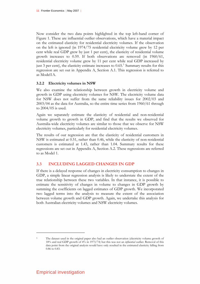
Figure 1 illustrates the relationship between GDP growth and electricity volume growth for residential and non-residential customers. The results of our regression are that the elasticity of residential electricity volumes (illustrated in blue) is estimated at 0.46. In contrast, the elasticity for non-residential electricity volumes (illustrated in red) is estimated at 1.04. Summary results for these regressions are set out in Appendix A, Section A.1. These regressions are referred to as Model1.

Residential vol growth = 3.3% + 0.46 GDP growth

R2 = 8%

Non-residential vol growth = 2.2%+ 1.04 GDP growth

R2 = 45%

-2%

0%

2%

4%

6%

8%

10%

12%

14%

-4% -2% 0% 2% 4% 6% 8%

Australian real GDP growth

Ele

ctric

ity v

olum

e gr

owth

Residential volume growthNon-residential volume growthLinear (Residential volume growth)Linear (Non-residential volume growth)

Figure 1: Relationship between growth in residential electricity consumption and real GDP growth



Now consider the two data points highlighted in the top left-hand corner of Figure 1. These are influential outlier observations, which have a material impact on the estimated elasticity for residential electricity volumes. If the observation on the left is ignored (in 1974/75 residential electricity volume grew by 12 per cent while real GDP grew by just 1 per cent), the elasticity of residential volume growth increases to 0.59. If both observations are removed (in 1960/61, residential electricity volume grew by 11 per cent while real GDP increased by just 3 per cent), the elasticity estimate increases to 0.65.5 Summary results for this regression are set out in Appendix A, Section A.1. This regression is referred to as Model1A.

3.2.2 Electricity volumes in NSW

We also examine the relationship between growth in electricity volume and growth in GDP using electricity volumes for NSW. The electricity volume data for NSW does not suffer from the same reliability issues for 2002/03 and 2003/04 as the data for Australia, so the entire time series from 1960/61 through to 2004/05 is used.

Again we separately estimate the elasticity of residential and non-residential volume growth to growth in GDP, and find that the results we observed for Australia-wide electricity volumes are similar to those that we observe for NSW electricity volumes, particularly for residential electricity volumes.

The results of our regression are that the elasticity of residential customers in NSW is estimated at 0.51, rather than 0.46, while the elasticity of non-residential customers is estimated at 1.43, rather than 1.04. Summary results for these regressions are set out in Appendix A, Section A.2. These regressions are referred to as Model 1.

3.3 INCLUDING LAGGED CHANGES IN GDP

If there is a delayed response of changes in electricity consumption to changes in GDP, a simple linear regression analysis is likely to understate the extent of the true relationship between these two variables. In that instance, it is possible to estimate the sensitivity of changes in volume to changes in GDP growth by summing the coefficients on lagged estimates of GDP growth. We incorporated two lagged terms into the analysis to measure the extent of the association between volume growth and GDP growth. Again, we undertake this analysis for both Australian electricity volumes and NSW electricity volumes.

5 The dataset used in the original paper also had an outlier observation (electricity volume growth of

18% and real GDP growth of 4% in 1973/74) but this was not an influential outlier. Removal of this data point from the original analysis would have only resulted in the estimated elasticity falling from 0.86 to 0.83.




For residential electricity volumes, the estimated relationship is summarised as follows:

21 38.027.048.0%57.0 −− +++= tttt ChgGDPChgGDPChgGDPChgvol

where:

Chgvolt = the percentage change in electricity volume in year t; and ChgGDPt-i = the percentage change in real GDP in year t-i for i = 0 to 2 (that is, the percentage change in GDP in the current year as well as the two prior years).

The sum of the coefficients on the three GDP terms is equal to 1.12, a figure which is insignificantly different from one.

We repeated this analysis for non-residential electricity consumption. For non-residential electricity volumes, the estimated relationship is summarised as follows:


The sum of the coefficients from this analysis is 1.22, which is also insignificantly different from one.

Thus, after incorporation of lagged GDP growth, the data does not imply any material difference in the association between volume growth and GDP growth for residential and non-residential customers. Furthermore, the data is consistent with a one-for-one relationship.

Summary results for these regressions are set out in Appendix A, Section A.1. These regressions are referred to as Model 2.


For residential electricity volumes, the estimated relationship is summarised as follows:


These results are similar to those for residential electricity volumes in Australia, with the sum of the coefficients on the three GDP terms equal to 1.20, rather than 1.12.

For non-residential electricity volumes, the estimated relationship is summarised as follows:



21 05.006.051.1%02.0 −− −++= tttt ChgGDPChgGDPChgGDPChgvol

Again, these results are quite similar to those for non-residential electricity volumes in Australia, with the sum of the coefficients on the three GDP terms equal to 1.51 instead of 1.22.


Comparing the results for residential and non-residential electricity volumes, it is apparent that the association between electricity volumes and GDP is more immediate for non-residential customers. The models for residential customers have higher coefficients on the lagged GDP terms and lower coefficients on the contemporaneous GDP figure, compared to the models for non-residential customers. But this does not necessarily imply that the true economic risk faced by the firms supplying residential customers is relatively lower; rather, it simply means that there may be a longer period of time between an unexpected change in GDP and unexpected change in volume.

3.4 INCLUDING LAGGED CHANGES IN VOLUME

An additional modification that can be incorporated into the analysis is to use previous changes in volume growth itself as an independent variable.

Our modelling of the representative firm incorporates contemporaneous changes in volume and the state of the economy. In a time-series of economic data, this systematic risk may not be observed at exactly the same time. There may be a lag between GDP growth and changes in electricity volume, especially where a residential customer delays engaging in energy-intensive activities (purchase of appliances and larger houses). This delayed response does not mean that systematic risk is any less. It simply means that we have to accumulate the systematic risk over these delayed responses. Once this is accounted for, we observe that there is approximately a one-for-one relationship between GDP growth and changes in electricity volume, for both residential and non-residential customers. Lagged terms are typically incorporated into the published research and are likely to explain why our estimated elasticities of close to one are higher than elasticities reported in those papers.

Again, we undertake this analysis for both Australian electricity volumes and NSW electricity volumes.




If the prior change in electricity volume is included as an independent variable, the estimated regression equation for residential customers is as follows:

121 51.021.006.043.0%38.0 −−− ++++−= ttttt ChgvolChgGDPChgGDPChgGDPChgvol

When interpreting the results from regression analysis, it is important to interpret the set of estimated coefficients jointly, not in isolation. Incorporating the additional last term into the regression equation makes it especially important not to separately interpret the individual coefficients resulting from the analysis. The last variable in the equation – volume growth observed in the previous year – is positively associated with the other variables in the equation. This introduces the statistical problem known as multicollinearity. When a regression equation contains independent variables that have a high degree of association with one another, we often observe a material increase in one coefficient and a material decrease in another coefficient. This can occur to the point where one coefficient becomes significantly negative and the other significantly positive, even though both variables are expected to have a positive relationship with the dependent variable.

However, we can jointly interpret the coefficients from the regression output and use these coefficients to model the relationship between unexpected economic growth and unexpected electricity volume growth. The output implies that residential electricity volume in one year is expected to grow by around seven-tenths of GDP growth over the previous three years (0.71 is the sum of the three coefficients relating to volume growth), plus around half of the previous year’s volume growth, minus a constant term of 0.4 per cent. (Of course, the previous year’s volume growth is itself associated with the previous GDP growth, so you see how it is important to interpret these coefficients in their entirety, and not focus on the coefficients in isolation.)

These coefficients jointly imply that, in high-growth states of the economy, electricity consumption growth is expected to grow at a slightly faster rate than GDP, while growing at a slightly lower rate in low-growth economic states. This occurs because there is a percentage increase in electricity volume of around two-fifths of GDP growth, plus the carryover from GDP growth from the previous two years, plus an additional increase equal to half the volume growth observed in the prior year (some of which is due to an increase in wealth and some of which is due to factors unrelated to GDP growth). In aggregate, this result remains consistent with an approximate one-for-one relationship between unexpected GDP growth and unexpected growth in residential electricity volume, as shown below.

To illustrate this relationship we performed a simulation analysis based upon the equation presented above. We simulated cumulative annualised volume growth and cumulative annualised GDP growth over a ten-year estimation window, after incorporating random fluctuations in volume growth and GDP growth based



upon the error terms resulting from the regression analysis. The ten-year estimation window was selected to capture the relationship between volume growth and lagged terms, as well as to be consistent with our prior modelling which relied upon a ten-year period. We repeated this simulation 100,000 times to directly observe the distribution of ten-year volume growth and GDP growth implied by the regression analysis.

Figure 2 illustrates the ratio of unexpected electricity volume growth to unexpected GDP growth over then ten-year estimation window. Simulated growth is expressed in percentage terms relative to its average on an annualised basis. It is important to express these growth figures relative to expectations because volume growth has outstripped GDP growth in historical terms – but this average higher growth doesn’t describe the relationship between the two variables. The distribution illustrated below has a median estimate of 1.2, consistent with an approximate one-for-one relationship between the two variables assumed in our analysis.

0.0

0.2

0.4

0.6

0.8

1.0

1.2

1.4

1.6

-20.0

-18.0

-16.0

-14.0

-12.0

-10.0 -8.

0-6.

0-4.

0-2.

0 0.0 2.0 4.0 6.0 8.0 10.0

12.0

14.0

16.0

18.0

20.0

Elasticity

Freq

uenc

y (%

)

Median = 1.2

Figure 2: Distribution of unexpected volume growth relative to unexpected GDP growth for residential electricity customers (Model 3)

This simulation analysis is purely a mechanism for interpreting the results of the regression analysis. It relies exclusively on the output from the historical data in order to directly address the issue at hand, and basically asks, “If expected volume growth is modelled according to the equation above, and potential random variation around this expected result is consistent with what we have observed before, what is the most likely relationship between unexpected volume growth and unexpected GDP growth?” The most likely outcome is approximately a one-for-one relationship.



We repeated the analysis using data relating to non-residential electricity consumption. Using this dataset, the estimated regression equation is as follows:

121 60.001.047.093.0%62.0 −−− ++−+= ttttt ChgvolChgGDPChgGDPChgGDPChgvol

As with the results from the residential volume dataset, we can jointly interpret the coefficients resulting from this output. Growth in non-residential electricity volume is expected to grow at roughly half the rate of average GDP growth over the prior three years (0.47 is the sum of the three coefficients on the growth terms), plus around three-fifths of the prior year’s volume growth, plus a constant term of 0.6 per cent. After simulating GDP growth and volume growth over a ten-year estimation period, according to these coefficients and including randomisation based upon the imprecision of the regression model, we computed volume growth relative and GDP growth relative to their average values. The ratio of these two figures has a median value of 1.1, as illustrated in Figure 3. This suggests there is no material difference in the sensitivity of changes in electricity volume growth for residential versus non-residential customers.

0.0

0.2

0.4

0.6

0.8

1.0

1.2

1.4

1.6

-20.0

-18.0

-16.0

-14.0

-12.0

-10.0 -8.

0-6.

0-4.

0-2.

0 0.0 2.0 4.0 6.0 8.0 10.0

12.0

14.0

16.0

18.0

20.0

Elasticity

Freq

uenc

y (%

)

Median = 1.1

Figure 3: Distribution of unexpected volume growth relative to unexpected GDP growth for non-residential electricity customers (Model 3)





Considering electricity volumes in NSW, if the prior change in electricity volume is included as an independent variable, the estimated regression equation for residential customers is as follows:

121 27.030.013.052.0%25.0 −−− ++++−= ttttt ChgvolChgGDPChgGDPChgGDPChgvol

As with the other results for residential electricity volumes, these results for NSW are not very different from the results for Australia. For NSW residential customers, the sum of the coefficients on GDP growth is 0.94 rather than 0.71, and the coefficient on lagged electricity volume is 0.27 rather than 0.51. As for residential electricity volumes in Australia, these results for NSW are close to one-for-one.

For non-residential customers in NSW, the estimated regression equation is as follows:

121 09.005.018.054.100.0 −−− −−++= ttttt ChgvolChgGDPChgGDPChgGDPChgvol

These results for NSW are quite different from the results for Australia, with higher coefficients on GDP, but a lower (negative) coefficient on lagged volume growth. Although, as discussed, it is important to be careful interpreting these coefficients in isolation because of the multi-collinearity of the variables.


3.5 INCLUDING ELECTRICITY PRICES

It would be expected that electricity prices would also have an impact on electricity volumes, so we investigate the impact of including prices in our models of electricity volumes. Since we have a time series of NSW electricity prices, we focus on modelling the impact on NSW electricity volumes.

For each of the models set out in the section above, we repeat our analysis with electricity prices included as a variable. For models of residential electricity volumes we include residential electricity prices, and for models of non-residential electricity volumes we include non-residential electricity prices. Summary results for these regressions are set out in Appendix A, Section A.3. The regressions are referred to as Models 4, 5 and 6 (which, except for the inclusion of price, correspond to Models 1, 2 and 3).

In general, we find that electricity prices are not, in themselves, significant. However, the inclusion of electricity prices improves the models of electricity volumes, both in terms of the joint significance of the explanatory variables and the goodness-of-fit of the overall model. Further, the price estimates obtained



from these models were of the expected negative sign, implying the estimated relationship is in the right direction, albeit not particularly strong.

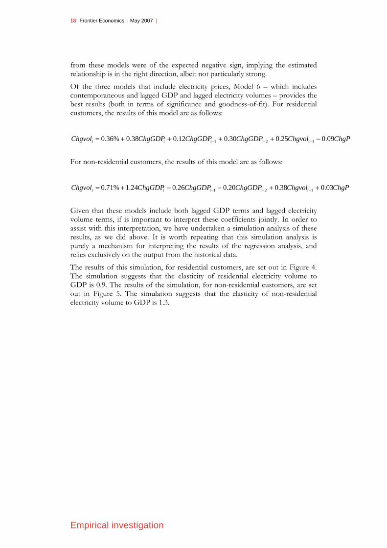
Of the three models that include electricity prices, Model 6 – which includes contemporaneous and lagged GDP and lagged electricity volumes – provides the best results (both in terms of significance and goodness-of-fit). For residential customers, the results of this model are as follows:

ChgPChgvolChgGDPChgGDPChgGDPChgvol ttttt 09.025.030.012.038.0%36.0 121 −++++= −−−

For non-residential customers, the results of this model are as follows:

ChgPChgvolChgGDPChgGDPChgGDPChgvol ttttt 03.038.020.026.024.1%71.0 121 ++−−+= −−−

Given that these models include both lagged GDP terms and lagged electricity volume terms, if is important to interpret these coefficients jointly. In order to assist with this interpretation, we have undertaken a simulation analysis of these results, as we did above. It is worth repeating that this simulation analysis is purely a mechanism for interpreting the results of the regression analysis, and relies exclusively on the output from the historical data.

The results of this simulation, for residential customers, are set out in Figure 4. The simulation suggests that the elasticity of residential electricity volume to GDP is 0.9. The results of the simulation, for non-residential customers, are set out in Figure 5. The simulation suggests that the elasticity of non-residential electricity volume to GDP is 1.3.



0.0

0.2

0.4

0.6

0.8

1.0

1.2

1.4

1.6

Elasticity

Median = 0.9

Figure 4: Distribution of unexpected volume growth relative to unexpected GDP growth for residential electricity customers (Model 6)

0.0

0.2

0.4

0.6

0.8

1.0

1.2

1.4

1.6

Elasticity

Median = 1.3

Figure 5: Distribution of unexpected volume growth relative to unexpected GDP growth for non-residential electricity customers (Model 6)



3.6 INCLUDING GAS PRICES

It is typical, when modelling demand for a product, to include own-prices and cross-prices as variables in the analysis. In particular, it is generally useful to include the prices of competing (i.e. substitute) products. In the case of electricity, the most obvious substitute is gas. For this reason we investigated the inclusion of gas prices in our modelling, to determine whether gas prices improved our models of electricity volumes.

The results were not encouraging. None of the models that incorporated gas prices provided statistically worthwhile results. The difficulty is most likely with the data on gas prices. Since natural gas has been available in NSW only since the late 1970s, the annual time series of gas prices only had about 20 observations, once a change series and lagged terms are accounted for. Our modelling suggests that such a short time-series does not provide reliable results in this case.

3.7 LONG RUN VS. SHORT RUN REACTIONS

Thus far the models have considered a long run relationship between electricity volume growth and GDP growth, not the short run elasticity. An econometric model class that is often used to describe the long and short run relationships between two time-series is a Vector Error-Correction Model (VECM). Models of this type assume there is a long run stable, or equilibrium, relationship between the time-series considered, and assume that deviations from this long run equilibrium are short term shocks. VECMs attempt to describe the short run adjustments to the long run equilibrium relationship. Estimation of VECMs is a much more complicated econometric exercise than the analysis carried out thus far. There are a few points worth noting about this kind of model when considering a VECM:

Before modelling a relationship as a VECM, it is important to have a strong theoretical case supporting a long run relationship between the time-series under consideration. In this case, it would be necessary to have a strong theoretical reason to believe that there exists a long run, stable, relationship between GDP growth, growth in electricity prices, and growth in electricity volume usage.

Before modelling a long run relationship, the time-series must be put through statistical tests to determine if they may indeed share a long-run trend or equilibrium. That is, VECMs are only appropriate to certain time-series.

To obtain good estimates of the short and long run adjustments of the time-series to movements in each other it is helpful to have relatively large sample sizes. Our sample is limited to around 42 annual observations, and is made shorter once lagged terms are included.

Given the reasons above, and the inability of our previous analysis to reject a one-for-one relationship (or, in many cases, a .75 relationship), we decided not to extend our analysis by estimating VECMs.



3.8 EMPIRICAL ANALYSIS CONCLUSION

On the basis of the empirical analysis that we have undertaken, we conclude that the best estimate of the relationship between residential electricity volumes and GDP growth is that the relationship is one-for-one.

As discussed, simple models that only include GDP growth and growth in electricity volumes suggest that the elasticity of volume growth to GDP growth may be significantly lower than one; the best estimate for residential customers based on these results suggest that the elasticity is 0.5. However, these simple models do not provide good results.

As the results set out in Appendix A reveal, including lagged GDP, lagged volume growth and electricity prices in the model of electricity growth improves the model. In fact, the best model that we tested included each of these terms, as well as contemporaneous GDP growth. For residential electricity volumes, the sum of the coefficients on GDP growth is 0.8 in this model. We tested the hypothesis that the sum of these coefficients is equal to one, and could not reject this hypothesis. We also tested the hypothesis that the sum of the coefficients on GDP growth is equal to 0.75 in this model, and also could not refect this hypothesis. In addition, however, this model has a positive coefficient of 0.25 on lagged electricity volume, which is in turn related to GDP growth. Our simulation of the results for this model suggests that the best estimate of the relationship between residential electricity volume and GDP growth is 0.9.

Other models also support the conclusion that the relationship between residential electricity volume and GDP growth is one-for-one, as clearly illustrated by the sum of the GDP coefficients for each model, set out in Appendix A. For example, if lagged electricity volume is excluded from the model, the sum of the coefficients on GDP growth is 1.03, and we cannot reject the hypothesis that the sum of the coefficients is equal to one. Again, however, we also cannot reject the hypothesis that the sum of the coefficients on GDP growth is equal to 0.75.

Given this evidence we cannot reject our null hypothesis that residential electricity volumes grow in proportion to the growth of the broader economy. We consider that the best interpretation of our empirical results is that the relationship between growth in residential electricity volume and growth in GDP is one-for-one.

The reason that the simple model that excludes lagged GDP suggests that the relationship is less than one-for-one appears to be explained by the coefficients on the lagged terms: the electricity use of residential customers appears to respond to changes in GDP over a couple of years, rather than immediately. Non-residential customers, in contrast, respond more quickly.

Before concluding, it is worth reiterating that we are attempting to make a judgment from just 44 annual observations of volume growth and GDP growth and performing analysis which does not incorporate one-off events which have the potential to impact on the results. In large samples, there is a reasonable presumption that this noise in the dataset will have minimal impact on the validity of the conclusions. That is, an outlier that is likely to bias the result in one



direction is likely to be offset by another outlier that has the opposite effect. This presumption is less reasonable in small samples.



References

References

Akmal, M. and Stern, D., 2001, Residential energy demand in Australia: An application of dynamic OLS, Working papers in Ecological Economics, Centre for Resource and Environmental Studies, ANU, No. 0104, 1-26.

Donnelly, W., 1984, Residential electricity demand modelling in the Australian Capital Territory: preliminary results, Energy Journal, 5, 119-131.

Donnelly, W. and Diesendorf, M., 1985, Variable elasticity models for electricity demand, Energy Economics, 7, 159-162.

Donnelly, W. and Saddler, H., 1984, The retail demand for electricity in Tasmania, Australian Economic Papers, 23, 52-60.

Hawkins, R., 1975, The demand for electricity: A cross-section study of New South Wales and the Australian Capital Territory, Economic Record, 51, 1-18.

Hickling, R., 2006, Electricity Consumption in New South Wales: An application of cointegration techniques to energy modelling and forecasting, TransGrid Economics Information Paper, 1-31.

Mahadevan, R. and Asafu-Adjaye, J., 2007, Energy consumption, economic growth and prices: A reassessment using panel VECM for developed and developing countries, Energy Policy, 35, 2481-2490.

Narayan, P.K. and Smyth, R., 2005, The residential demand for electricity in Australia: An application of the bounds testing approach to cointegration, Energy Policy, 33, 467-474.

Rushdi, A., 1986, Interfuel substitution in the residential sector of South Australia, Energy Economics, 8, 177-185.


Appendix A

A.1 MODELS OF AUSTRALIAN ELECTRICITY VOLUMES

Data/Variable Model1 Res Model1 Non-Res Model1A Res Model2 Res Model2 Non-Res Model3 Res Model3 Non-Res

chGDP co-efficient 0.46 1.04 0.65 0.48 1.05 0.43 0.93standard error 0.24 0.18 0.21 0.23 0.20 0.20 0.17p value 0.06 0.00 0.00 0.05 0.00 0.04 0.00

L.chGDP co-efficient 0.27 0.11 0.06 -0.47standard error 0.24 0.20 0.21 0.22p value 0.26 0.58 0.78 0.04

L2.chGDP co-efficient 0.38 0.06 0.21 0.01standard error 0.23 0.20 0.20 0.16p value 0.11 0.77 0.30 0.95

L.chResD co-efficient 0.51standard error 0.14p value 0.00

L.chNonResD co-efficient 0.60standard error 0.15p value 0.00

Cons co-efficient 0.03 0.02 0.02 0.01 0.01 0.00 0.01standard error 0.01 0.01 0.01 0.01 0.01 0.01 0.01p value 0.00 0.01 0.02 0.67 0.20 0.75 0.52

r2 8.3% 45.3% 20.0% 24.3% 47.6% 45.7% 64.6%p 0.06 0.00 0.00 0.02 0.00 0.00 0.00

SumGDPcoeff 0.46 1.04 0.65 1.12 1.22 0.71 0.46

Appendix A


A.2 MODELS OF NSW ELECTRICITY VOLUMES

Data/Variable Model1 Res Model1 Non-Res Model2 Res Model2 Non-Res Model3 Res Model3 Non-Res

chGDP co-efficient 0.51 1.43 0.57 1.51 0.52 1.54standard error 0.27 0.31 0.26 0.34 0.25 0.34p value 0.07 0.00 0.03 0.00 0.05 0.00

L.chGDP co-efficient 0.24 0.06 0.13 0.18standard error 0.26 0.34 0.26 0.43p value 0.37 0.86 0.62 0.68

L2.chGDP co-efficient 0.39 -0.05 0.30 -0.05standard error 0.25 0.33 0.25 0.33p value 0.13 0.87 0.24 0.89

L.chResD co-efficient 0.27standard error 0.15p value 0.08

L.chNonResD co-efficient -0.09standard error 0.20p value 0.65

chResP co-efficientstandard errorp value

chNonResP co-efficientstandard errorp value

Cons co-efficient 0.03 0.01 0.00 0.00 0.00 0.00standard error 0.01 0.01 0.01 0.02 0.01 0.02p value 0.01 0.68 0.94 0.99 0.86 1.00

r2 8% 33% 22% 36% 28% 36%p 0.07 0.00 0.02 0.00 0.01 0.00

SumGDPcoeff 0.51 1.43 1.20 1.51 0.94 1.67

Appendix A


A.3 MODELS OF NSW ELECTRICITY VOLUMES – WITH PRICES

Data/Variable Model4 Res Model4 Non-Res Model5 Res Model5 Non-Res Model6 Res Model6 Non-Res

chGDP 0.29 1.38 0.42 1.42 0.38 1.240.32 0.25 0.30 0.26 0.30 0.260.37 0.00 0.18 0.00 0.21 0.00

L.chGDP 0.23 0.21 0.12 -0.260.27 0.26 0.27 0.320.40 0.43 0.64 0.42

L2.chGDP 0.38 -0.16 0.30 -0.200.25 0.25 0.25 0.240.14 0.55 0.25 0.41

L.chResD 0.250.150.10

L.chNonResD 0.380.160.03

chResP -0.14 -0.09 -0.090.13 0.12 0.120.28 0.44 0.46

chNonResP 0.04 0.05 0.030.05 0.05 0.050.41 0.36 0.55

Cons 0.04 0.01 0.01 0.00 0.00 0.010.01 0.01 0.02 0.0.00 0.35 0.63 0.

10% 43% 23% 48% 0.12 0.00 0.05 0.00 0.03 0.00

umGDPcoeff 0.29 1.38 1.03 1.47 0.80 0.78

01 0.02 0.0178 0.81 0.61

r2 29% 55%p

S

Appendix A


Appendix A


The Frontier Economics Network

Frontier Economics Limited in Australia is a member of the Frontier Economics network, which consists of separate companies based in Australia (Melbourne, Sydney & Brisbane) and Europe (London & Cologne). The companies are independently owned, and legal commitments entered into by any one company do not impose any obligations on other companies in the network. All views expressed in this document are the views of Frontier Economics Pty Ltd.

Disclaimer

None of Frontier Economics Pty Ltd (including the directors and employees) make any representation or warranty as to the accuracy or completeness of this report. Nor shall they have any liability (whether arising from negligence or otherwise) for any representations (express or implied) or information contained in, or for any omissions from, the report or any written or oral communications transmitted in the course of the project.


THE FRONTIER ECONOMICS NETWORK

MELBOURNE | SYDNEY | BRISBANE | LONDON | COLOGNE | BRUSSELS

Frontier Economics Pty Ltd, 395 Collins Street, Melbourne 3000

Tel. +61 (0)3 9620 4488 Fax. +61 (0)3 9620 4499 www.frontier-economics.com

Documents

Relationship between GDP and electricity demand