The GDP-Temperature Relationship: Implications for Climate

The GDP-Temperature Relationship: Implications for Climate Change DamagesRichard G. Newell, Brian C. Prest, and Steven E. Sexton

Working Paper 18-17 REV July 2018; revised November 2018

The GDP-Temperature Relationship: Implications for

Climate Change Damages

Richard G. Newell Brian C. Prest Steven E. Sexton ∗

November 16, 2018

∗Newell: Resources for the Future, 1616 P St NW, Washington, DC 20036; Duke University

(email: [email protected]). Prest: Resources for the Future, 1616 P St NW, Washington, DC 20036

(email: [email protected]). Sexton: Duke University, 201 Science Drive, Durham, NC 27708, (email:

[email protected]).

The GDP-Temperature Relationship: Implications for

Climate Change Damages

November 16, 2018

Abstract

A growing literature characterizes climate change damages by relating temperature shocks

to GDP. But theory does not clearly prescribe estimable forms of this relationship, yielding dis-

cretion to researchers and generating potentially considerable model uncertainty. We therefore

employ model cross validation to assess the out-of-sample predictive accuracy of 400 variants

of prominent models, identify the set of superior models, and characterize both model and

sampling uncertainty. Estimates of GDP impacts vary substantially across models, especially

those assuming temperature effects on GDP growth, rather than levels. The best-performing

models have non-linear temperature effects on GDP levels, and imply global GDP losses of

1-2% by 2100.

1 Introduction

It has long been understood that economic outcomes are related to climate. This climate-economy

relationship determines the scope and magnitude of market impacts from climate change over the

next 100 years and beyond. Consequently, an understanding of the climate-economy relationship is

central to projections of damages from anticipated climate change, and to policymaking that weighs

the benefits and costs of climate change mitigation. Yet estimation of the scope and magnitude of

climate impacts on the economy is hindered by the temporal invariance of climate over relevant

time frames. The relationship between economic outcomes and cross-sectional climate variation is

confounded by regional heterogeneity, including historical effects of settlement and colonization

(e.g., Acemoglu et al. 2002; Easterly and Levine 2003; Rodrik et al. 2004; Dell et al. 2014).

A recent literature, therefore, employs panel econometric methods to estimate the response of

economic outcomes to weather, which is commonly defined as realizations from distributions of

climatic variables, like temperature, wind, and precipitation (Dell et al. 2014; Hsiang 2016). This

literature has estimated economically and statistically significant effects of weather on specific

subsectors of the economy, such as crop yields, industrial output, and labor productivity.1 A subset

of this literature also relates weather and weather shocks to economic aggregates like gross domestic

product (GDP) (Hsiang 2010; Barrios et al. 2010; Anttila-Hughes and Hsiang 2011; Deryugina

2011; Dell et al. 2012; Hsiang and Narita 2012; Burke et al. 2015, 2018).

Much of this empirical research is intended to inform estimation of climate change damages and

determinations of efficient climate change mitigation programs (Dell et al. 2014; Deryugina and

Hsiang 2014; Hsiang 2016; National Academies of Sciences 2017; Burke et al. 2018). Integrated

assessment models (IAMs), commonly used in analysis of climate change mitigation costs and

benefits, rely upon the enumeration and aggregation of relevant, sector-specific impacts (National

Academies of Sciences 2017). Given the sparseness of empirical estimates of sectoral impacts

around the world, such models often must rely on extrapolation out of sample. Therefore, growing

1See for instance Deschenes and Greenstone (2007); Schlenker and Roberts (2009); Schlenker and Lobell (2010);Feng et al. (2010); Jones and Olken (2010); Lobell et al. (2011); Cachon et al. (2012); Fisher et al. (2012); Dell et al.(2014); Graff Zivin and Neidell (2014).

1

interest centers on the econometric estimation of climate impacts on economic aggregates that

subsume sectoral effects, obviating the need to fully enumerate and estimate them. The aggregate

econometric approach also complements the enumerative approach by validating estimated magni-

tudes of damages. However, economic aggregates such as GDP are not direct welfare measures,

and do not reflect non-market values affected by climate change that should be included in welfare

analysis.

The aggregate econometric approach has faced at least two important limitations. First, using

weather variation to identify climate effects requires strong assumptions about dynamic processes

like adaptation and the persistence of idiosyncratic temperature responses amid secular climate

change (Dell et al. 2014; Hsiang 2016). Second, theory does not prescribe specific, estimable,

structural relationships between climate and economic outcomes (Dell et al. 2014; Hsiang 2016;

Schlenker and Auffhammer 2018). Researchers, therefore, have made varying assumptions about

the functional forms of these relationships. The importance of those assumptions for understanding

the estimated impact of warming on GDP has not yet been evaluated. As we show in this paper,

these assumptions substantially influence predicted economic losses from climate warming.

Dell et al. (2012), henceforth DJO, estimated that rich country GDP growth is unaffected by

temperature, while poor country growth is adversely affected by positive temperature shocks. They

did so by relating country-level, aggregate per-capita economic growth to a log-linear function

of temperature and precipitation, controlling for time-invariant country heterogeneity and secular

trends. Such results corroborate the view that industrialized countries are relatively less affected by

climate change because their economies are less exposed to weather and their capacities to adapt to

change are greater (Poterba 1993; Mendelsohn et al. 1994; Kahn 2005; Stern 2006; Nordhaus 2008;

Tol 2009; Deryugina and Hsiang 2014).

In contrast to DJO, Burke et al. (2015), henceforth BHM, specified a quadratic relationship

between temperature and per capita GDP growth that suggests rich and poor countries alike

suffer from global warming and that both agricultural and industrial output growth are impeded.

Controlling for a quadratic of precipitation, time-invariant country heterogeneity, secular trends, and

2

parametric country-specific quadratic trends, the preferred model of BHM predicts global income

losses of 23% by 2100 due to unmitigated climate change. BHM also report that the responsiveness

of economic growth to temperature is persistent across their fifty-years of observation, implying

little historical adaptation to temperature shocks and supporting an interpretation of the weather

effects they estimated as a lower bound on climate impacts. Burke et al. (2018) employ the same

econometric framework as BHM to estimate that a cumulative $20 trillion in global damages would

be avoided by 2100 by limiting climate change to 1.5◦Celsius (C), rather than 2◦C.

Whereas DJO and BHM each estimate a relationship between temperature and GDP growth,

Hsiang (2010) and Deryugina and Hsiang (2014) postulated a non-linear relationship between

temperature and GDP levels.2 The magnitude of the threat to global wealth posed by climate change

varies dramatically according to these competing models. BHM estimate that country-level GDP

growth is maximized at an annual average temperature of 13◦C, whereas Hsiang (2010) estimates

no significant effects of weather on contemporaneous production in developing country contexts

until daily average temperatures exceed 27◦C. Yet Deryugina and Hsiang (2014) estimate GDP

losses beyond even moderately warm daily temperatures in the United States.

We show that estimates of the GDP-maximizing temperature vary considerably across alternative

specifications of the GDP-temperature relationship. Many estimates of this GDP-maximizing annual

average temperature fall in the range of 13-15◦C at which the bulk of production occurs today. Thus,

an assessment of the relative performance of alternative models and of the magnitude of model

uncertainty is critical to determining the capacity of this aggregate econometric approach to improve

understanding about the scope and magnitude of future climate change damage.

Economists have long observed that theory often does not precisely define estimable forms

of economic relationships, reserving to empiricists significant discretion in defining functional

2Hsiang (2010) relied principally upon a linear model to identify statistically and economically significant effects ofannual average temperature on aggregate output and sectoral production in the Caribbean and Central America. Hisestimation of a piece-wise linear function relating daily average temperature to annual production indicated productionlosses occur only on extremely hot days with average temperatures of 27-29◦C. Specifying a similar piece-wise linearrelationship between daily temperatures and GDP levels, Deryugina and Hsiang (2014) estimated U.S. productionlosses at daily average temperatures as low as 15◦C.

3

forms and selecting conditioning variables.3 The consequences of that selection for inference

have also long been enumerated.4 As Hendry (1980) and Leamer (1983) observed, given that

parameter sensitivity is indicative of specification error, empiricists often endeavor to demonstrate

the robustness of parameter estimates to alternative assumptions. Yet, as Leamer (2010) contends,

such sensitivity analyses or robustness checks are themselves often performed in ad hoc ways.

Rigorous model selection tools can be applied in these settings to empirically ground model selection

via processes less dependent upon researcher discretion.

Using rigorous model selection procedures, this paper systematically assesses the sensitivity

of temperature parameter estimates to modeling assumptions and considers the implications of

model uncertainty for estimates of the GDP impacts from climate change. It evaluates competing

models in the literature and a range of variants using the methods of model cross validation that are

advocated for predictive models and for causal inference.5

Whereas the previous climate-economy literature has selected preferred models using in-sample

fit criteria that are subject to the well-known over-fitting critique, we evaluate models according

to out-of-sample model fit criteria, as is particularly appropriate for models that are intended to

predict future economic outcomes given expectations about future climatic conditions. Moreover,

we invoke the substantial literature on data-driven, predictive model comparison (e.g., White 1996;

Diebold and Mariano 1995; Hansen 2005; Hansen et al. 2011) to identify the set of models that are

statistically superior to alternatives. This approach is standard (e.g., Diebold and Mariano 1995;

West 1996), and was employed by Auffhammer and Steinhauser (2012) in the related context of

modeling carbon emissions in the United States.

We use a country-level panel of economic growth, temperature, and rainfall to estimate the

global relationship between GDP and temperature. Four hundred models are estimated. They

vary along three key dimensions: the assumed functional form for temperature and precipitation,

3For example, see Friedman (1953); Dhrymes et al. (1972); Cooley and LeRoy (1981); Leamer (1978, 1983); White(1996); Yatchew (1998); Hansen et al. (2011), and Belloni et al. (2014).

4See Keynes (1939), Koopmans (1947), Leamer (1978), Leamer (1983), Hendry et al. (1990), Chatfield (1996), andSullivan et al. (1999), among others.

5For example, Friedman (1953); Varian (2014); Kleinberg et al. (2015); Christensen and Miguel (Forthcoming), andAthey (2017).

4

methods of controlling for potentially confounding time trends, and the choice of GDP growth or

levels as the relevant dependent variable. These models are evaluated by several cross-validation

techniques to determine their relative performance, as well as their implications for damages from

future warming.

Cross validation and statistical tests of model superiority reveal considerable model uncertainty

that implies GDP impacts by 2100 ranging from substantial losses to substantial gains. The models

performing best in cross validation specify a nonlinear (quadratic or cubic) temperature function,

though these are not statistically significantly better than models excluding temperature or specifying

it as a linear or piece-wise linear function. The model preferred by BHM that predicts GDP losses

of 23% performs more poorly, in a statistically significant sense, than dozens of alternatives.

Models with the lowest root mean squared error in cross validation posit a relationship between

temperature and GDP levels, not GDP growth. These models imply global GDP losses from unmiti-

gated warming of 1-2% by 2100. Across all GDP-levels models of statistically indistinguishable

performance, the range of estimated climate impacts is similarly narrow.

Nonetheless, we cannot statistically reject the possibility that the best-performing model is one

relating temperature to GDP growth. However, growth models yield immense uncertainty about

global warming impacts. Across just those growth models that specify a non-linear temperature

function, the combined model and sampling uncertainty yield a standard deviation of predicted

impacts equal to 108% of GDP, with model uncertainty being a somewhat larger component relative

to sampling uncertainty.6 Models specifying impacts on GDP levels, not growth, yield far less

uncertainty in climate impacts; the standard deviation is equal to less than 1% of GDP for model,

sampling, and combined uncertainty. Considerable growth model uncertainty affords little policy

guidance and suggests caution is warranted when such estimates are incorporated into IAMs (e.g.,

6Growth models imply a range of impacts that is implausibly large given the overall historical exposure of theeconomy to temperature. The agricultural sector, for example, is one of the most exposed to climate change, butrepresents only a few percent of global income, whereas about two-thirds is services. Assumptions about the impact ofdiscontinuous, catastrophic climate damages have been considered on the order of tens of percent (Kopits et al. 2014),but these types of impacts are not reflected in the historic data on which the GDP-temperature relationship is estimated.

5

Moore and Diaz 2015). Levels models, in contrast, are associated with less model uncertainty and

project a range of impacts consistent with damage estimates embodied in leading IAMs.

Informed by cross validation, we assess heterogeneity of temperature impacts across rich

and poor countries and across agriculture and non-agriculture sectors. Though parameters of the

disaggregated temperature functions imply a concave relationship as in the aggregate results, the

statistical significance and robustness of effects is diminished at the sectoral level, particularly for

rich countries. We find evidence of a statistically significant and robust quadratic relationship only

among poor country agricultural production.

The paper is organized as follows. The next section reviews the literature on the relationship

between temperature and economic aggregates, highlighting the variety of modeling assumptions

employed in the literature. Section 3 describes our method of assessing the impact of these

alternative assumptions, and section 4 presents results of the model cross validation and implications

for causal inference and climate damage projections. Section 5 concludes.

2 Estimating Economic Responses to Climate Change

Research on agriculture, human capital, and other specific impacts of climate and temperature

provide the microeconomic foundation for aggregate economic effects. These microeconomic

foundations characterize a non-linear relationship between temperature and economic outcomes,

with significant adverse production impacts occurring at daily average temperatures above about

29◦C.7 It also demonstrates the alternative choices researchers have made in modeling the tempera-

ture relationship. The most flexible specifications of the micro-foundations literature use binned

temperature observations to flexibly model non-linear relationships; but bin widths vary across these

papers. Researchers have also considered the impacts of temperature and climate on human health,

conflict, and violence; factors that affect welfare, but less directly impact aggregate production.

7See Schlenker and Roberts (2009); Graff Zivin and Neidell (2014), and Sudarshan et al. (2015).

6

The first estimates of the global welfare impacts of climate change were produced in the 1990s

by combining assumptions about the extent of future warming with scientific evidence of its physical

impacts and their valuation (Fankhauser 1994; Nordhaus 1994; Tol 1995, 2002a,b; Fankhauser

2013). This approach is embodied in three reduced-form IAMs that have informed the social cost

of carbon in the United States (National Academies of Sciences 2017). This enumerative method

contrasts with the statistical method employed by Mendelsohn et al. (2000a) and Mendelsohn et al.

(2000b) and later Maddison (2003) and Nordhaus (2006) that inferred climate change costs from

variation in economic activity across climates.

Central estimates across these early studies range from a -11.5% loss of global GDP to a slight

gain of 0.1% for temperature increases of 2.5-5.4◦C relative to pre-industrial levels (Tol 2014).

Most models, including the IAMs used to estimate the U.S. social cost of carbon, predict losses of a

few percent of GDP from a few degrees of warming (Greenstone et al. 2013; Tol 2014; Nordhaus

and Moffat 2017). Whereas the enumerative approach of the IAMs accounts for non-market impacts

and affords damage estimates that are traceable to specific mechanisms, it may overlook some

channels by which climate change affects the economy, and it may extrapolate impacts out of sample

to heterogeneous regions and production (Dell et al. 2012; Carleton and Hsiang 2016; National

Academies of Sciences 2017).

More recent statistical approaches mitigate omitted variables bias in the early work, which had

only exploited cross-sectional variation in climate. They do so by observing economic responses

to weather (i.e., short-term variations in climate), which varies also in the temporal dimension,

allowing the use of fixed effects to control for time-invariant region heterogeneity. This strand of

the literature includes Hsiang (2010), DJO, Hsiang and Jina (2014), Deryugina and Hsiang (2014),

BHM, and Burke et al. (2018). Though these papers all relate economic outcomes to temperature

shocks, they differ in how they specify the equations used to estimate these responses. There are

three principal model variations we explore: (1) GDP level or growth effects; (2) temperature

functional form; and (3) controls for unobserved trends.

7

GDP Level or Growth Effects. There is disagreement in the recent empirical literature as to

whether temperature affects the level of economic output or its growth (e.g., see Schlenker and

Auffhammer 2018). The modeling choice is not a trivial one. Growth effects compound over

time, whereas level effects do not. Thus, predictions of future losses from climate change vary

considerably depending upon whether growth or level models are specified. The micro-foundations

literature has largely related temperature to levels of economic outcomes, not their growth (Dell

et al. 2012, Burke and Emerick 2015). The temperature impacts it documents, e.g., yield losses

and reduced labor supply, are widely-accepted determinants of GDP. IAMs also relate temperature

to levels of output, as do some econometric models of economic aggregates (National Academies

of Sciences 2017, Hsiang 2010, Deryugina and Hsiang 2014). In contrast, DJO, BHM, Hsiang

and Jina (2014), and Burke et al. (2018) propose growth may be affected beyond impacts on

contemporaneous output.

The recent empirical literature does not provide strong theoretical foundations to favor models

relating temperature to growth or levels. DJO characterize output as a multiplicative function

of population, labor productivity, and exponentiated temperature. They offer the intuition that

temperature may affect institutions, which may affect productivity growth. BHM propose output is

a function of temperature and total productive capacity, which depreciates over time and is rebuilt

by savings. Savings, they assume, are permanently diminished during periods of high temperature

and attendant low output. BHM also suggest that the rate of technological change is slowed by

diminished cognitive capacity due to temperature change. These mechanisms are plausible, but

have attracted little attention in the growth literature.

Whether temperature shocks permanently affect savings or some other determinant of growth is

ultimately an empirical question that DJO and BHM each consider. Each examines the effect of

temperature lags on GDP growth rates. DJO report results from models that include one, five, and

ten-period lags of temperature (and precipitation in some specifications). In each of these models,

the contemporaneous effect of temperature on growth is negative and statistically significant among

poor countries. The first temperature lag in each model exhibits the opposite sign. Though the

8

first-lag coefficients are not statistically significant and are equal in magnitude to only approximately

one-half to one-third of the contemporaneous effect, such sign reversal is indicative of temporary

effects rather than persistence. This is particularly true given serial correlation in country average

annual temperatures that implies a relatively hot year is typically followed by another relatively hot

year, e.g., due to El Nino-Southern Oscillation and other decadal oscillations (Hsiang 2010).8 Such

serial correlation inhibits immediate recovery from a temperature shock and confounds efforts to

determine the cumulative effect of a given pulse of hot weather. It tends to bias lagged coefficients

in favor of persistence over transience and makes it unlikely a level effect would produce first-lag

coefficients of common magnitude and opposite sign. Regardless, lagged-effects models typically

admit the decay or growth of impulse effects over time, but not sign reversals.9

Similarly, BHM estimate distributed lag models with 1-5 lags of a quadratic temperature

polynomial to explore the persistence of temperature effects. In none of these BHM models is the

cumulative temperature effect on growth statistically distinguishable from zero, indicating against

growth effects. The sign on the coefficients of the first lag of temperature and squared temperature

are always opposite the sign of the corresponding contemporaneous effects, in an offsetting manner.

And the lagged effects are always approximately half as large as the contemporaneous effects.10 In

the one-lag model of BHM, lagged temperature and squared temperature coefficients are statistically

significant. In all lagged models of BHM, either the first or second lag of temperature and squared

temperature is statistically significant and opposite the contemporaneous effects in sign. Such sign

8In BHM data, the first lag and contemporaneous temperature have a correlation coefficient of 0.5. This correlationis depicted for each country in Appendix Figure A1. Contemporaneous temperature and more distant lags are alsopositively correlated, though, as expected, the correlation declines with lag distance.

9DJO interpret their lagged-effects models differently than we do because they assume a transitory contemporaneoustemperature effect on GDP growth and a lagged temperature effect on GDP level. See their equation (2). This assumptionis strong, and seems counter to the intuition they provide—that temperature may affect institutions that affect growth. Ifinvestment in institutions is low relative to some counterfactual during a temperature shock, then institutional investmentremains low indefinitely in subsequent periods unless an offsetting temperature shock occurs. Thus, a temperatureshock that affects GDP growth should affect growth in subsequent periods, producing lagged temperature effects thatexhibit common sign and magnitudes to the contemporaneous effect. The sum of all temperature coefficients, then,should exceed the magnitude of the contemporaneous effect. Yet none of the lagged temperature coefficients in DJOmodels is statistically significant at conventional levels. All are small in magnitude, and the sum of coefficients issmaller in magnitude than the contemporaneous effect. This suggests the absence of persistent temperature effects ongrowth, contrary to the interpretation of DJO.

10BHM do not report these coefficients in their main text or supplementary information. We produced the coefficientsand their standard errors using BHM replication data and code.

9

reversals are not indicative of persistent effects.11 BHM interpret these results cautiously: “Thus,

while we can clearly demonstrate that there is a non-linear effect of temperature on economic

production, we cannot reject the hypothesis that this effect is a true growth effect nor can we reject

the hypothesis that it is a temporary level effect.”

Given the empirical ambiguity of persistent growth effects and the absence of theoretical

foundations, there is no clear rationale for choosing to model temperature effects on GDP growth

or GDP levels. Estimating a model with GDP growth as the dependent variable addresses the

non-stationarity of the GDP series. But that solution does not obligate a model relating GDP growth

to temperature levels. Rather, it is common to difference the right-hand side and the left-hand side

of an equation relating GDP levels to predictors by subtracting the expression for a one-period lag

of GDP level as in, e.g., Mankiw et al. (1992) and Bernanke and Gurkaynak (2001).

Temperature Functional Form. The second dimension along which the climate-economy lit-

erature varies is specification of the function relating temperature to economic outcomes. This

choice also dramatically affects the magnitude of damage estimates. DJO model a linear temper-

ature effect, implying that a temperature shock affects economic outcomes similarly regardless

of the mean from which temperatures deviate. In a model that controls for time-invariant country

heterogeneity, region-specific trends, and unique temperature responses for rich and poor countries,

they estimate that temperature has no statistically significant effect on growth among rich countries.

Among poor countries, however, it causes a statistically and economically significant reduction

in contemporaneous growth, which declines by 1.4 percentage points annually for each 1◦C of

warming.

In contrast, BHM favor a quadratic relationship between temperature and growth that allows

warming to boost growth in countries with cold climates and impede growth in hot countries.

Using data substantially similar to DJO, they estimate statistically and economically significant

growth effects of temperature shocks in rich and poor countries alike, and across both agricultural

11The addition of temperature lags to the models that perform best in our model cross validation also yields littleevidence of persistent temperature effects.

10

and industrial production.12 The quadratic specification estimated by BHM identifies an optimal

annual average temperature for GDP growth of 13◦C from which deviations in either direction

generates changes in growth of equal magnitude but opposite sign. The quadratic temperature

relationship is more flexible than the linear relationship specified by DJO. Yet it imposes a symmetry

of growth effects due to temperature deviations away from the optimum that abstracts from the

micro foundations evidence.13

BHM also consider higher-ordered polynomials of temperature, as well as restricted cubic

splines with 3-7 knots. These alternative specifications all confirm a concave relationship between

temperature and growth, but the peaks of the concave relationships vary across specifications in

non-trivial ways. The alternative models typically imply a GDP-maximizing temperature greater

than 13◦C. Hsiang (2010) and Deryugina (2011) also implement more flexible, piece-wise linear

functions of temperature that accommodate asymmetric effects of small increases and decreases in

temperature relative to an optimum.

DJO also implement the micro-response approach of binning daily temperatures to non-

parametrically estimate the temperature-growth relationship. While cautioning against over-

interpretation due to data reliability concerns, they nevertheless report in an online appendix

estimated coefficients that characterize approximately linear effects that are statistically indistin-

guishable from zero for poor countries across all temperature bins. For rich countries, temperature

coefficients are approximately zero and not statistically significant, except in the range of 15-25◦C,

within which coefficients are positive and barely significant.

12BHM impose a globally quadratic relationship, not to be confused with a within-country quadratic relationship. Asshown by McIntosh and Schlenker (2006), these two assumptions are conceptually different on a fundamental level, and,therefore, have significant practical implications. For example, a global quadratic implies a single centering point (here,“GDP-maximizing temperature”) for all countries and years, compared to many country- and year-specific centeringpoints.

13BHM state conditions under which the annual aggregation of daily temperatures used in some of the micro-foundations literature (e.g., Schlenker and Roberts 2006, Graff Zivin and Neidell 2014, Sudarshan et al. 2015, Stevens2017) yields a temperature response curve that is concave, smoother, and characterized by a lower optimum temperaturethan the micro responses. It is also important to note that some of the micro-foundations literature relates outcomesto daily maximum temperature, which is characterized by a higher mean than daily, monthly, or annual averagetemperatures that incorporate temperature readings from relatively cool nighttime periods. However, the concaverelationship BHM define in their equation (1) does not impose symmetry. See their figure 1(f).

11

Controls for Unobserved Trends. The third major dimension of model heterogeneity within the

existing literature is the choice of controls for trending unobservables. DJO employ country fixed

effects, year fixed effects interacted with regional indicators, and year fixed effects interacted with

an indicator for countries that are poor when they enter the data.14 This saturates the model with

fixed effects to non-parametrically control for unobservables. It is robust to region-specific time

trends that might be unique to rich or poor countries.

BHM prefer a model less saturated with fixed effects, and instead parametrically control for

country-specific time trends. Like DJO, they use country fixed effects to control for time-invariant

country heterogeneity. They also use a set of year fixed effects to control for global trends in growth.

Rather than controlling for regional or country-type (e.g., poor) trends non-parametrically as in

DJO, BHM introduce a parametric country-specific quadratic time trend. Because the dependent

variable in their regressions, growth, is the first derivative of income, their quadratic trend implies a

country-specific cubic polynomial in income levels. BHM report that estimation results look similar

with only a linear trend in growth. However, as we show in this paper, estimated GDP impacts vary

considerably across alternative specifications.

Hsiang (2010) includes country and industry-specific quadratic time trends in his models

of the production responses to temperature change in 28 Caribbean-basin countries. He also

includes industry-region-year and industry-country fixed effects, yielding a level of fixed effects

saturation more similar to DJO than to BHM. Because GDP growth is the first derivative of income

levels, the quadratic time trend in Hsiang (2010) is analogous to a linear time trend in a growth

model, distinguishing it from the quadratic-in-growth trend employed by BHM. Also distinct

from BHM, Hsiang and Jina (2014) include a linear country-specific time trend in estimating the

relationship between economic growth and cyclone exposure in the Caribbean. This imparts a

quadratic time effect in levels of production, similar to Hsiang (2010). They also include year fixed

effects to flexibly control for common trends and country fixed effects to control for time-invariant

heterogeneity. Deryugina and Hsiang (2014) exclude parametric time trends in estimating the

14“Poor” is defined as per capita GDP below the country median at the earliest period recorded.

12

production responses of U.S. counties as a flexible function of temperature. They use county and

year fixed effects to control for common trends and time-invariant county heterogeneity.

Theory offers little guidance in controlling for trending unobservables, and the extant literature

appears to take a fairly ad hoc approach to modeling trend heterogeneity. Because of heterogeneity

in endowments, institutions, and history, countries or regions are likely to have varying growth

capabilities. The parametric trends employed by BHM and Hsiang and Jina (2014) permit country-

level heterogeneity. They estimate GDP effects of temperature from deviations in country-specific

growth trends. But the temporal heterogeneity is introduced in a constrained manner. Such

parametric trends can result in over-fitting, as we demonstrate they do in this setting.15 Fixed effects

flexibly and non-parametrically control for trends, but they do not admit country-specific trends.

Models saturated with fixed effects lend credible causal inference as they are robust to many sources

of omitted variables bias, but they may also absorb variation necessary to identify some relationships

(e.g., Fisher et al. 2012; Deschenes and Greenstone 2012).16 In the present context, saturation of

fixed effects or parametric time trends can both lead to this problem; DJO include 300 region-year

fixed effects that BHM do not, whereas BHM include 332 time trend variables not included in DJO.

Table 1 summarizes the varying assumptions of prominent papers in the climate-economy

literature along key dimensions. The cross validation exercise described in the subsequent section

considers the sensitivity of temperature parameters to modeling assumptions along these dimensions.

3 Data and Methods

Given the model uncertainty evident in the growing climate econometrics literature, empiricists

must make choices about functional forms and inclusion or exclusion of controls. Such model

uncertainty is important to the extent that outcomes of interest differ markedly across alternative

15Two of the models we consider in this study include removing the country-specific quadratic time trends fromBHM’s specification as well as adding them to DJO’s specification. As shown in Section 4, both of these alternativespecifications change the sign of the estimated impacts of warming on GDP in 2100.

16As discussed by Fisher et al. (2012), oversaturation of fixed effects can amplify attenuation bias in the presence ofmeasurement error. Too many controls will absorb most of the variation in the data, leaving measurement error to playa larger role in the remaining identifying variation.

13

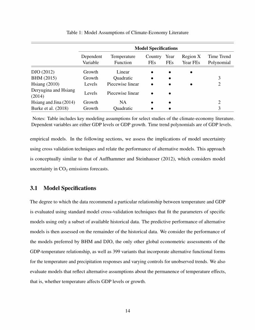
Table 1: Model Assumptions of Climate-Economy Literature

Model Specifications

DependentVariable

TemperatureFunction

CountryFEs

YearFEs

Region XYear FEs

Time TrendPolynomial

DJO (2012) Growth Linear • • •BHM (2015) Growth Quadratic • • 3Hsiang (2010) Levels Piecewise linear • • • 2Deryugina and Hsiang(2014)

Levels Piecewise linear • •

Hsiang and Jina (2014) Growth NA • • 2Burke et al. (2018) Growth Quadratic • • 3

Notes: Table includes key modeling assumptions for select studies of the climate-economy literature.Dependent variables are either GDP levels or GDP growth. Time trend polynomials are of GDP levels.

empirical models. In the following sections, we assess the implications of model uncertainty

using cross validation techniques and relate the performance of alternative models. This approach

is conceptually similar to that of Auffhammer and Steinhauser (2012), which considers model

uncertainty in CO2 emissions forecasts.

3.1 Model Specifications

The degree to which the data recommend a particular relationship between temperature and GDP

is evaluated using standard model cross-validation techniques that fit the parameters of specific

models using only a subset of available historical data. The predictive performance of alternative

models is then assessed on the remainder of the historical data. We consider the performance of

the models preferred by BHM and DJO, the only other global econometric assessments of the

GDP-temperature relationship, as well as 399 variants that incorporate alternative functional forms

for the temperature and precipitation responses and varying controls for unobserved trends. We also

evaluate models that reflect alternative assumptions about the permanence of temperature effects,

that is, whether temperature affects GDP levels or growth.

14

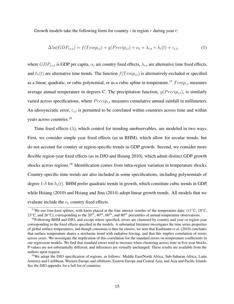
Growth models take the following form for country i in region r during year t:

∆ ln(GDPi,r,t) = f(Tempi,t) + g(Precipi,t) + αi + λr,t + hi(t) + εi,t, (1)

where GDPi,r,t is GDP per capita, αi are country fixed effects, λr,t are alternative time fixed effects,

and hi(t) are alternative time trends. The function f(Tempi,t) is alternatively excluded or specified

as a linear, quadratic, or cubic polynomial, or as a cubic spline in temperature.17 Tempi,t measures

average annual temperature in degrees C. The precipitation function, g(Precipi,t), is similarly

varied across specifications, where Precipi,t measures cumulative annual rainfall in millimeters.

An idiosyncratic error, εi,t is permitted to be correlated within countries across time and within

years across countries.18

Time fixed effects (λ), which control for trending unobservables, are modeled in two ways.

First, we consider simple year fixed effects (as in BHM), which allow for secular trends, but

do not account for country or region-specific trends in GDP growth. Second, we consider more

flexible region-year fixed effects (as in DJO and Hsiang 2010), which admit distinct GDP growth

shocks across regions.19 Identification comes from intra-region variation in temperature shocks.

Country-specific time trends are also included in some specifications, including polynomials of

degree 1-3 for hi(t). BHM prefer quadratic trends in growth, which constitute cubic trends in GDP,

while Hsiang (2010) and Hsiang and Jina (2014) adopt linear growth trends. All models that we

evaluate include the αi country fixed effects.

17We use four-knot splines, with knots placed at the four interior ventiles of the temperature data: (11◦C, 18◦C,23◦C, and 26◦C), corresponding to the 20th, 40th, 60th, and 80th percentiles of annual temperature observations.

18Following BHM and DJO, and except where specified, errors are clustered by country and year or region-yearcorresponding to the fixed effects specified in the models. A substantial literature investigates the time series propertiesof global surface temperatures, and though consensus is thus far elusive, we note that Kaufmann et al. (2010) concludesthat surface temperature shares a stochastic trend with radiative forcing, and that this implies correlation of errorsacross years. We investigate the implication of this correlation for the standard errors on temperature coefficients inour regression models. We find that standard errors tend to increase when clustering across time in five-year blocks.P-values are not substantially different, and inferences are virtually unchanged. These results are available from theauthors upon request.

19We adopt the DJO specification of regions, as follows: Middle East/North Africa, Sub-Saharan Africa, LatinAmerica and Caribbean, Western Europe and offshoots, Eastern Europe and Central Asia, and Asia and Pacific Islands.See the DJO appendix for a full list of countries.

15

The models preferred by BHM and DJO are versions of (1). BHM regress log-GDP growth on

a quadratic of temperature and precipitation, year and country fixed effects, and country-specific

quadratic trends. DJO specify log-GDP growth as a function of temperature and country, region-year,

and poor-year fixed effects.20

Because GDP (in levels) is a non-stationary series, we specify a GDP level response to tempera-

ture in first differences. This results in the same regressand as the growth model in (1). Distinct

from (1), however, the values of temperature and precipitation enter as first differences, rather than

levels.21 Hence, the levels-versus-growth distinction can be interpreted as an alternative function

f(Tempi,t). For example, if the temperature response of (log) GDP levels is thought to be quadratic,

i.e.,

ln(GDPi,r,t) = β1Tempi,t + β2Temp2i,t + · · · ,

then the first-differenced, stationary, and estimable relationship is:

∆ ln(GDPi,r,t) = β1∆Tempi,t + β2∆[Temp2i,t] + · · · , (2)

which uses growth rates (log-differences of per capita GDP) as the dependent variable. The final

term is the change in temperature-squared, which we note is conceptually very different from the

squared change in temperature, i.e., (∆Tempi,t)2. If this is the data-generating process, it can be

estimated by regressing growth on the corresponding first-difference of the specified temperature

response, i.e., ∆f(Tempi,t).

As demonstrated in the subsequent section, the models favored by CV are versions of (2). They

relate the first difference of log-GDP per capita to the first difference of temperature and squared

temperature and include country and region-year fixed effects.22 Superior-performing models in

20Poor-year fixed effects are interactions of year indicators and an indicator for whether a country was poor when itentered the data, defined as per capita GDP below the median.

21While BHM (and DJO) note the non-stationarity concern and, hence, the need to take first differences, they onlytake first differences in the left-hand side of the equation, GDP, without taking first differences in the right-hand side(temperature and precipitation). Consequently, their estimated models are not directly derived from their conceptualmodels.

22One of the models favored by CV admits the first difference of temperature cubed.

16

cross validation exercises that account for the time-series nature of the GDP and temperature series

exclude any function of precipitation and any parametric trends.

The models we evaluate include the preferred model of BHM, where f(Tempi,t), g(Precipi,t),

and hi(t) are quadratic functions and λr,t is a simple year fixed effect. Because we employ

the same data as BHM, as detailed in the subsequent subsection, we can replicate BHM and

evaluate their model relative to alternatives. Also included among the evaluated models is the

preferred specification of DJO, which interacts linear temperature responses and region-specific

fixed effects with an indicator of whether the corresponding country is “poor”. Despite using the

same specification as in DJO, we estimate coefficients that differ slightly from those in DJO because

we employ the more recent data used in BHM. These include ten additional years of data relative to

DJO.23

In total, we evaluate 401 possible specifications, including DJO’s preferred specification (which

is not nested in the model space due to “poor” country interactions with time fixed effects and the

temperature function). The other 400 model variations result from the following modeling choices:

• GDP growth versus level effect (2 forms): f(Tempi,t) versus ∆f(Tempi,t);

• Temperature function (5 forms): none, 1-3 degree polynomials, or spline;

• Time and region controls (8 forms)

– Time fixed effects (2 forms): simple year (BHM-style) or region-year (DJO-style); and

– Country-specific time trends (4 forms): none and 1-3 degree polynomials.24

• Precipitation function (5 forms): none, 1-3 degree polynomials, or spline.

3.2 Data

Models are estimated using the same data employed by BHM. Specifically, we use the 2012 World

Development Indicators (World Bank 2012) country-year panel of real annual GDP per capita for

23We are nevertheless able to replicate DJO on the data used by DJO.24All time trends are referenced according to the order of the polynomial as it would appear in the growth model,

i.e., equation (2). Hence, a “linear” time trend enters a GDP growth equation as a linear trend and corresponds to aquadratic time trend in GDP levels.

17

166 countries from 1960 to 2010. The data include 6,584 country-year observations.25 Also as in

BHM, we use Matsuura and Willmott (2012) gridded, population-weighted average temperature

and precipitation data aggregated to the country-year level.

While only GDP, temperature, and precipitation data are used for estimation, we also forecast

the GDP impacts of the alternative parameter estimates using the same method as BHM. As in BHM,

projections of population and economic growth are drawn from the Shared Socioeconomic Pathways

(O‘Neill et al. 2014) scenario 5 (SSP5). For comparison to BHM, we use the representative carbon

pathway RCP8.5 as a benchmark scenario of unmitigated future warming (van Vuuren et al. 2011).

It represents the ensemble average of all global climate models contributing to CMIP5, the Coupled

Model Intercomparison Project phase 2010-2014 that informed the fifth assessment report of the

Intergovernmental Panel on Climate Change.26 RCP8.5 corresponds to an expected increase of

4.3◦C in global mean surface temperature by 2100 relative to pre-industrial levels (Stocker et al.

2013).

3.3 Cross Validation Techniques

Given theoretical ambiguity about which econometric models correctly capture the data generating

process, model performance is a useful criterion for model selection. As Hsiang (2016) notes,

the parameters empirically recovered in climate econometric models are “put to work” in order

to “inform projections of future outcomes under different climate scenarios.”27 Consequently, the

out-of-sample prediction properties of models are arguably the performance characteristics of

primary importance.

In-sample fit criteria are prone to selecting over-fitted models, particularly as high-ordered

polynomials of covariates are introduced in some models (Chatfield 1996). Commonly reported

25The panel is not balanced because the data series is not complete for the full period for some countries. In particular,some countries are added to the series post-1960.

26See http://cmip-pcmdi.llnl.gov/.27For instance, such parameter estimates can be used to generate estimates of the net present value of future damages

from emitting a ton of greenhouse gases. These estimates of the social cost of carbon are used to evaluate the benefitsof carbon reductions (National Academies of Sciences 2017).

18

http://cmip-pcmdi.llnl.gov/

statistics, like adjusted R2, Akaike Information Criterion (AIC), and Bayesian Information Criterion

(BIC) assess in-sample model fit with parametric penalties for the inclusion of weakly correlated

covariates. Each has flaws (Green 2012). Therefore, we employ model cross-validation (CV) to

assess the performance of alternative models of the GDP and temperature relationship. By training

the model over a subset of the data, the training set, and assessing its predictive accuracy on a

hold-out sample, the test set, the CV approach is expressly non-parametric and avoids the ad hoc

penalties of alternative, in-sample measures of model performance (Stone 1974, Snee 1977).28

Out-of-sample validation is not a new approach and the literature has a rich history (e.g., Diebold

and Mariano 1995; West 1996). In a study related to climate change specifically, Auffhammer

and Steinhauser (2012) used such an approach to evaluate competing models for CO2 emissions

forecasts.

We undertake cross validation of the DJO and BHM models, and 399 alternatives, using three

CV methods that divide data into distinct training and test sets. These three methods are: forecast,

backcast, and K-fold CV. Forecast CV explicitly accounts for the time-series nature of the dataset,

dividing the historical data into training sets of early data and testing on later data.29 This is a

standard and intuitive approach for evaluating the out-of-sample performance of statistical models

of time series data. Raftery et al. (2017), for instance, use this method to evaluate the performance

of forecasts of GDP per capita, population, and carbon emissions. Backcast CV is similar to forecast

CV, but implemented by training on the most recent data and testing on early data.30 K-fold CV

proceeds by dividing the data randomly into K groups and iteratively training the model K times on

K−1K

of the data. The model estimated in each iteration is tested on the remaining 1K

of the data.31

28See also Arlot and Celisse (2010) for a more recent survey.29We implement forecast CV using eight training windows that begin in 1961 and end, respectively, in 1970, 1975,

1980, 1985, 1990, 1995, 2000, and 2005. Each test period begins in the year following the end of the training windowand spans five years, e.g., 1971-1975, 1976-1980, etc. For all cross-validation methods, we drop countries with fewerthan 10 years of data in the training set to avoid bias in the specification of flexible time trends.

30Eight Backcast CV training windows are used, each ending in 2010 and beginning in 1966, 1971, 1976, 1981,1986, 1991, 1996, and 2001, respectively. Each test period spans the five years preceding the beginning of the trainingwindow (e.g., 1961-1965, 1966-1970, 1971-1975, etc.).

31We set K = 5, as is common in the literature. Thus, a given model is estimated each time using 4/5 of the data, andits accuracy is tested on the remaining 1/5 (Geisser 1975). This process is repeated 5 times, so that every observationis used in a test set exactly once. K-fold CV is conceptually similar to leave-one-out CV, but less computationallyintensive. Using multiple splits avoids the randomness inherent in splitting the data only once (Opsomer et al. 2001).

19

We implement K-fold CV, despite being ill-suited for time series data, in an effort to be complete

and avoid researcher discretion. K-fold CV ignores the time-series nature of the data, providing

an optimistic estimate of model fit if data are serially correlated by fitting to test observations that

are dependent upon the training observations. It also does not extrapolate out of sample where

over-fitted models perform poorly.

When econometric models include fixed effects, cross validation methods may not generate

parameter estimates for fixed effects appearing in test data that do not appear in training data. For

example, a model estimated on 1961-1980 data will have no estimated fixed effect for the year 1981

that appears in a forecast CV test set. Auffhammer and Steinhauser (2012) address this problem by

estimating a linear trend in the fixed effects of the trained model and predicting on test data using

extrapolated fixed effects.

We adopt a different approach. We remove fixed effects from the models prior to estimation

by demeaning both the dependent and explanatory variables. This results in precisely the same

coefficient estimates on the remaining parameters, such as the coefficients on temperature. We

demean GDP growth and all explanatory variables (temperature, temperature squared, precipitation,

precipitation squared, the country-specific time trend polynomials, etc.) by the fixed effect groups.

This involves demeaning by both country and year (or region-year, in the case of the DJO-style

fixed effects) before implementing the CV.32,33

The random sampling to divide the observations is not block sampled because doing so would make it impossible toestimate certain coefficients such as country-specific time trends. In the event a training set incorporates no observationsfor a given country, observations for that country are omitted from the test set.

32Because the panel is not balanced, simply demeaning first by country and then by year does not produce a demeaneddataset. Therefore, we demean the data by employing the method of alternating projections. In particular, we use thedemeanlist() function from the R package lfe. Importantly, all polynomials and spline bases are computed priorto the demeaning process, including the first difference of these bases for the GDP levels specification. Failure to do sowould result in different coefficient estimates for the temperature relationship (among others) under the demeaning andindicator variable approaches.

33One may think any model with flexible region-year fixed effects will inevitably outperform counterparts that onlyinclude year fixed effects because we demean the fixed effects ex ante. In fact, this is not the case because coefficientson the other covariates vary differently depending on what variation remains after the fixed effects are removed. Inother words, the ex ante demeaning of fixed effects removes variation that would be obsorbed by the fixed effects in theestimation stage. Indeed, models with region-year FE fixed effects often under-perform their year FE counterparts whentime trends are included (see Tables 2 and 3.) Models with region-year fixed effects are not mechanically superior.

20

3.4 Projections of GDP Impacts of Climate Change

As in BHM, we project the impact of expected warming on global GDP by 2100 using the RCP8.5

climate projection as a benchmark of unmitigated climate change and SSP5 for projections of

moderate to strong baseline GDP and population growth (O‘Neill et al. 2014). Neither we nor BHM

forecast baseline GDP using the econometric model. Country-level projections of economic growth,

population growth, and climate warming are combined with the estimated relationship between

GDP growth and temperature to predict changes in future growth rates for each country and year.

Given the estimated concave growth-temperature relationship, baseline GDP growth is incremented

in cold countries as warming occurs and decremented in hot countries. We employ the methodology

and data of BHM’s preferred projection, so our GDP impact estimates nest theirs precisely. For a

more detailed description of this projection, see section D of BHM’s supplementary information.

Following BHM, we allow per capita GDP to evolve according to:

GDPi,t = GDPi,t−1 × (1 + ηi,t + δi,t) ,

where ηi,t is the economic growth rate absent temperature change from the SSP. The term δi,t is the

temperature-induced increment (or decrement) to growth due to temperature changes from country-

specific recent historical averages. Specifically, it evolves according to δi,t = f(Ti,t+) − f(Ti),

where Ti,t+ is projected temperature beyond 2010 and Ti is country-specific average temperature

from 1980-2010.34 Temperature deviations are estimated by assuming a linear increase from the

historical average to country-specific temperature projections in 2100 from the RCP8.5.

BHM demonstrate the uncertainty of GDP climate impacts by bootstrapping the estimation of

the growth-temperature relationship. In their preferred specification they find that approximately

30% of bootstrapped simulations yielded positive global GDP gains from projected warming in

2100 even though the central estimate was a 23% loss. This demonstrates the substantial sample

uncertainty over future climate change damages attributable to uncertainty over parameters. We also

34For models that relate GDP levels and temperature, we similarly increment or decrement growth based on the fittedmodel, which as shown in equation (2) relate growth rates to changes in temperature.

21

estimate the magnitude of sample uncertainty, but we uniquely relate it to model uncertainty, i.e.,

that uncertainty attributable to ambiguity about the correct model. As reported in the next section,

model uncertainty is shown to dominate even the substantial sample uncertainty BHM estimate,

unless one focuses solely on models that relate non-linear temperature to GDP levels.

4 Results

This section presents the results of the cross validation exercise, comparing the cross-validated

root-mean-square errors (CV RMSEs) across all 400 models. We then illustrate the estimated

relationships between GDP and temperature across all models favored in the previous literature

and those favored by cross validation. The estimated GDP impact in 2100 under each model

specification is illustrated for the benchmark scenario of unmitigated warming. Finally, impact

heterogeneity across rich and poor countries and across agricultural and non-agricultural production

is explored.

4.1 Model Cross-Validation

Employing cross validation by three distinct methods across 400 models results in 1,200 estimates

of RMSE. We focus attention on the subset of models that nest BHM and that include the models

favored by CV. Thus, we report results of each CV method for all models that include either a

quadratic of precipitation or exclude precipitation (yielding lowest RMSE). The RMSE for each

model i is calculated as RMSEi =√n−1

∑t e

2i,t =

√n−1

∑t(Yi,t − Yi,t)2, using the actual and

predicted values from the test set Yi,t and Yi,t, respectively.

4.1.1 Forecast CV

Forecast cross validation reveals that dozens of alternative models are characterized by similar

predictive ability as summarized by RMSE. These results are reported in Table 2 for models that

include a quadratic of precipitation (as BHM do) and in Table 3 for models that exclude precipitation

22

(as the superior models do). In fact, the lowest 50% of model RMSEs are between 0.0499 and

0.0673. For comparison, the sample standard deviation of GDP growth is 0.0615. As shown later in

this section, common predictive ability yields a large set of models of superior predictive ability

that is statistically indistinguishable across models in the set. This, combined with sensitivity

of projected GDP losses from warming, implies tremendous model uncertainty that is further

considered later in this section.

The best-performing model in forecast CV is one that relates GDP levels to a temperature

quadratic and region-year fixed effects, as reported in Table 3. This model yields an RMSE of

0.0499, 15% smaller than the RMSE of the BHM model reported in Table 2. For the best-performing

model, RMSE is invariant (to four decimal places) to changes in the temperature specification or its

exclusion from models. In fact, for any model that excludes parametric time trends, RMSE varies

by less than 0.0001 across alternative specifications of the temperature function.

Models that include flexible time trends perform poorly in cross validation relative to models that

exclude them. This is indicative of over-fitting. In fact, forecast CV prediction errors are minimized

by excluding time trends irrespective of other modeling assumptions. The inferior out-of-sample fit

among models with time trends (as in BHM) is notable because BHM indicate their preference for

quadratic time trends is partly due to in-sample prediction accuracy. Forecast CV results illustrate

that in-sample predictive accuracy can give a misleading view of out-of-sample validity.

Within the model space, performance of a model similar to DJO is assessed. The model, DJO∗,

adopts the DJO specification excepting interactions of a “poor” country indicator with temperature

and year effects. It specifies a linear temperature relationship, region-year fixed effects, and omits

country-specific time trends. As reported in Table 3 (and highlighted in blue text), the RMSE of

DJO∗ is 0.0501, comparable to that of DJO. A model that incorporates a quadratic temperature

function to DJO∗, which we call “DJO∗ + Quad. Temp”, yields a similar RMSE that is highlighted

in violet text in Table 2.

23

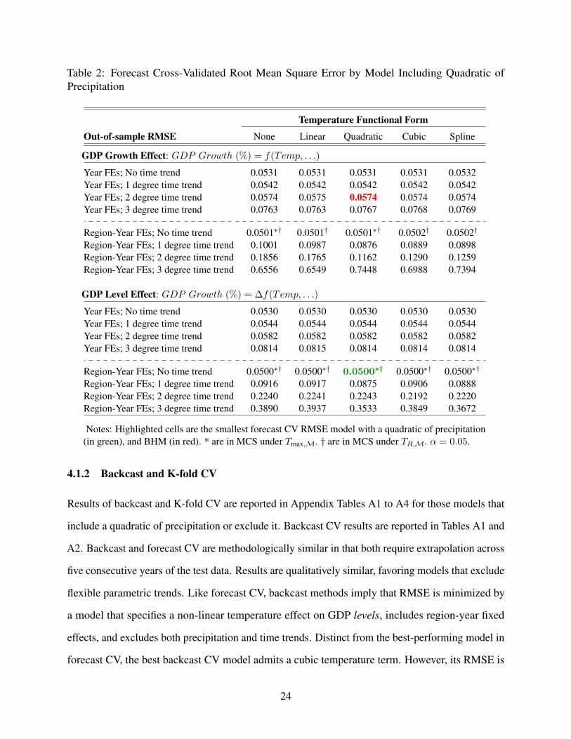
Table 2: Forecast Cross-Validated Root Mean Square Error by Model Including Quadratic ofPrecipitation

Temperature Functional Form

Out-of-sample RMSE None Linear Quadratic Cubic Spline

GDP Growth Effect: GDP Growth (%) = f(Temp, . . .)

Year FEs; No time trend 0.0531 0.0531 0.0531 0.0531 0.0532Year FEs; 1 degree time trend 0.0542 0.0542 0.0542 0.0542 0.0542Year FEs; 2 degree time trend 0.0574 0.0575 0.0574 0.0574 0.0574Year FEs; 3 degree time trend 0.0763 0.0763 0.0767 0.0768 0.0769

Region-Year FEs; No time trend 0.0501∗† 0.0501† 0.0501∗† 0.0502† 0.0502†

Region-Year FEs; 1 degree time trend 0.1001 0.0987 0.0876 0.0889 0.0898Region-Year FEs; 2 degree time trend 0.1856 0.1765 0.1162 0.1290 0.1259Region-Year FEs; 3 degree time trend 0.6556 0.6549 0.7448 0.6988 0.7394

GDP Level Effect: GDP Growth (%) = ∆f(Temp, . . .)


Region-Year FEs; No time trend 0.0500∗† 0.0500∗† 0.0500∗† 0.0500∗† 0.0500∗†


Notes: Highlighted cells are the smallest forecast CV RMSE model with a quadratic of precipitation(in green), and BHM (in red). * are in MCS under Tmax,M. † are in MCS under TR,M. α = 0.05.

4.1.2 Backcast and K-fold CV

Results of backcast and K-fold CV are reported in Appendix Tables A1 to A4 for those models that

include a quadratic of precipitation or exclude it. Backcast CV results are reported in Tables A1 and

A2. Backcast and forecast CV are methodologically similar in that both require extrapolation across

five consecutive years of the test data. Results are qualitatively similar, favoring models that exclude

flexible parametric trends. Like forecast CV, backcast methods imply that RMSE is minimized by

a model that specifies a non-linear temperature effect on GDP levels, includes region-year fixed

effects, and excludes both precipitation and time trends. Distinct from the best-performing model in

forecast CV, the best backcast CV model admits a cubic temperature term. However, its RMSE is

24

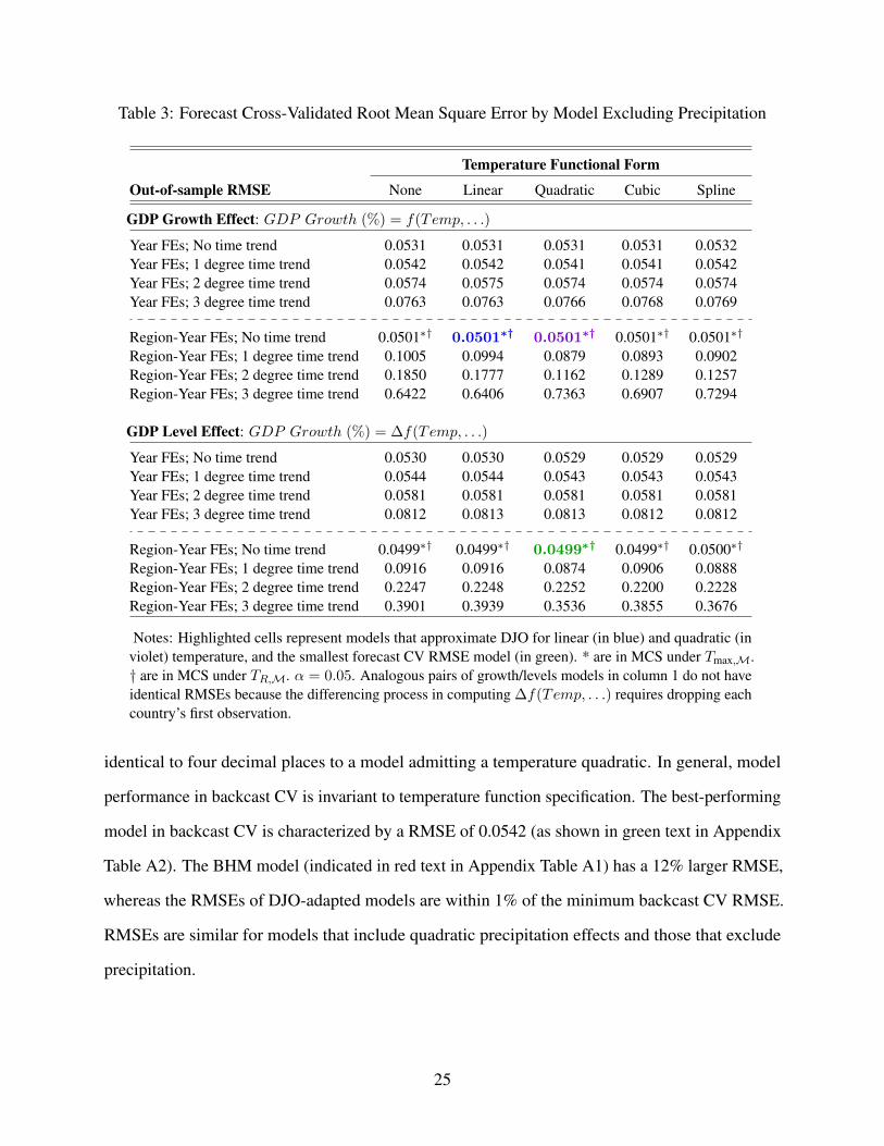
Table 3: Forecast Cross-Validated Root Mean Square Error by Model Excluding Precipitation











Notes: Highlighted cells represent models that approximate DJO for linear (in blue) and quadratic (inviolet) temperature, and the smallest forecast CV RMSE model (in green). * are in MCS under Tmax,M.† are in MCS under TR,M. α = 0.05. Analogous pairs of growth/levels models in column 1 do not haveidentical RMSEs because the differencing process in computing ∆f(Temp, . . .) requires dropping eachcountry’s first observation.

identical to four decimal places to a model admitting a temperature quadratic. In general, model

performance in backcast CV is invariant to temperature function specification. The best-performing

model in backcast CV is characterized by a RMSE of 0.0542 (as shown in green text in Appendix

Table A2). The BHM model (indicated in red text in Appendix Table A1) has a 12% larger RMSE,

whereas the RMSEs of DJO-adapted models are within 1% of the minimum backcast CV RMSE.

RMSEs are similar for models that include quadratic precipitation effects and those that exclude

precipitation.

25

Prediction errors across models in K-fold CV vary little, but best-performing models are similar

to those identified by forecast and backcast CV. For models that include a quadratic of precipitation

(see Appendix Table A3), RMSEs vary from 0.0508 to 0.0562 and equal 83-91% of the sample

standard deviation of GDP growth. None of the models provides a substantially better prediction of

future GDP growth across a randomly withheld 1/5th of the data than does the sample mean of GDP

growth. Because K-fold CV does not account for the time-series nature of GDP and temperature

series, these results are presented in the appendix only for completeness.

4.1.3 Model Confidence Sets

Given common CV performance across many models, a determination of which models are statisti-

cally significantly superior to alternatives in their predictive ability is not obvious. Therefore, and

given ex ante theoretical ambiguity about estimable relationships, we employ the model confidence

set (MCS) procedure of Hansen et al. (2011), which iteratively eliminates from consideration

models that are inferior to alternatives in their predictive ability at the 95% confidence level. Models

remaining under consideration are statistically indistinguishable in their performance. The proce-

dure considers a null hypothesis that model losses (prediction errors) are equivalent across models.

If the null is rejected, an elimination rule removes a model from consideration and the null is tested

again. The procedure iterates until the equivalence of model losses cannot be rejected.

Like Hansen et al. (2011), we consider two alternative elimination rules defined by alternative

test statistics. The first, denoted, test statistic Tmax,M, iteratively eliminates the model with the

greatest standardized loss relative to the average of models remaining in the consideration set. This

test results in a MCS comprised of 33, 158, and 209 models across the forecast, backcast, and K-fold

CVs, respectively. The alternative test, TR,M removes on each iteration the model that contributes

the greatest standardized loss with respect to any model in the consideration set. This alternative test

yields confidence sets comprised of 50, 151, and 55 models for each CV method, respectively. The

MCS is analogous to a confidence interval on a parameter estimate in that it is assured to contain

the best-performing model at a given confidence level. Like the confidence interval on a parameter

26

estimate, the greater size of the MCS reflects the limited information in the data with which to

discern among models. Hence, the large MCSs we identify reflect limitations of the data that lend

greater uncertainty to which is the best model. This is a unique characteristic of the MCS relative to

other tests of superior predictive ability (Hansen et al. 2011).

Models retained in the MCS are indicated in Tables 2-3 and A1-A4 by asterisks or daggers

(†) for the Tmax,M and TR,M statistics, respectively. The MCSs identified by forecast CV RMSEs

are exclusively comprised of models including region-year fixed effects, as in DJO, and excluding

parametric time trends preferred by BHM. The MCS, however, does not discern among temperature

functional forms or growth and level effects. The forecast MCSs contain models including all

temperature and precipitation specifications, as well as models that specify growth and GDP levels

relationships. The MCSs selected by backcast CV RMSEs are even less discerning among models.

This is evident by the large size of the confidence sets. They are predominated by models including

region-year fixed effects, but they also include some models that do not condition at all upon

heterogeneous trends. They exclude models that add parametric time trends in the absence of

region-year fixed effects (as in BHM). Like the forecast CV MCSs, the backcast CV MCSs include

models using any of the temperature specifications we evaluate. They also include growth and

GDP levels models. The model preferred by BHM is excluded from all MCSs. The DJO* and

DJO*+Quad. Temp. models are included in all forecast and backcast CV models.

4.1.4 Summary of CV Results

We conclude the following from CV and MCS analyses:

1. Dozens of alternative models exhibit comparable predictive ability in cross validation. This

leads to large sets of similarly-performing models characterized by statistically indistinguish-

able predictive ability.

2. The best-performing models relate GDP levels to temperature, not growth. But we cannot

preclude with 95% confidence that a model relating GDP growth to temperature is superior.

27

3. All models that minimize prediction errors across the CV procedures include non-linear

functions of temperature. However, we cannot preclude at the 95% confidence level that the

most predictive model excludes temperature or adopts any of the temperature functions we

considered. The invariance of RMSE to temperature specification is, perhaps, unsurprising

given the multiple factors determining GDP and its growth and the relatively small share

of variation explained by temperature.35 Model predictive ability is also invariant to the

specification of the function relating precipitation to GDP or GDP growth.

4. The models that perform best in forecast cross validation are exclusively those that include

region-year fixed effects to control for heterogeneous time trends (as in DJO) and exclude

parametric time trends (such as those included in the preferred model of BHM).

5. The model preferred by BHM is excluded from all MCSs.

4.2 Regression Estimates

In this section, we present parameter estimates from the models that minimize RMSE for each CV

method. For comparison purposes, we also report parameter estimates from the DJO and BHM

specifications, as well as those from two models that modify the DJO specification. These two

models omit poor-country interactions and include either a linear temperature effect (DJO*) or a

quadratic temperature effect (DJO*+Quad. Temp.). Table 4 reports parameter estimates for these

seven models.

As shown in columns 1 and 3, models favored by forecast and K-fold CV identify statistically

significant concave functions relating temperature to GDP levels. The model favored by backcast

CV also identifies a concave relationship, though the coefficient on the quadratic temperature term is

not statistically significant (see column 2). The fitted relationships of these and the other non-linear

models evaluated are shown in Appendix Figure A2. A concave relationship is common across

35A linear function of temperature explains only 0.2% and 0.03% of sample variation in GDP and GDP growth,respectively, conditional on region-year and country fixed effects. Even allowing for the non-linear effects of temperature,a flexible four-knot cubic spline of temperature explains only 0.9% and 0.4% of GDP and GDP growth variation,respectively.

28

these models. Like DJO, our DJO* model estimates a statistically insignificant temperature effect

on GDP growth (see columns 5 and 6), whereas our DJO*+Quad. Temp. specification identifies a

statistically significant concave relationship (column 7).

The models favored by CV (columns 1-3) imply smaller GDP impacts from warming than

estimated by BHM (column 4). This is largely because the models specify effects on GDP levels

rather than GDP growth. But the smaller GDP losses also reflect smaller temperature coefficients in

absolute value than those estimated by BHM. This yields a less concave temperature function than

in BHM.

The GDP-maximizing temperature implied by the temperature coefficients of each model is

reported below the coefficient estimates in Table 4. For the quadratic models, this peak is computed

as a−2b where a and b are the coefficients on the linear and quadratic terms, respectively. The models

preferred by forecast and backcast CV identify temperature optima of 13.9◦C and 16◦C, respectively.

The optimum estimated by BHM is 13.1◦C (55◦F). DJO’s linear specification naturally implies

no optimum, but the addition of a quadratic term to the adapted DJO specification (DJO*+Quad.

Temp.) produces a concave curve with a peak at 17◦C (63◦F). Though this adapted DJO model with

quadratic temperature does not minimize RMSE in any of our three CV approaches, it dominates the

BHM model in each. The differences across models in estimated temperature optima are substantial

and imply substantial variation in estimated climate change impacts. The location of the peak

determines whether many large economies are operating below the GDP-maximizing temperature

and, therefore, would have higher GDP from warming.36

Table 4 also reports a 95% quantile range of a bootstrapped distribution of temperature optima.

This provides a measure of variance in the temperature optima due to sampling uncertainty.37 For

all models, the range of temperatures reflected in the 95% quantile intervals indicates a substantial

36Average temperatures in the three largest economies in 2010—the United States, Japan, and China—were about14◦C, above BHM’s 13◦C peak (implying damages from 2◦C of warming) but below the “DJO+Quad” peak of 17◦C(implying benefits from the same amount of warming). These three economies collectively accounted for over 40% ofglobal GDP in 2010.

37The bootstrap procedure is described in section 4.3 under Sampling and Modeling Uncertainty. We report the 95%quantile range rather than standard errors because the distribution of the peak is non-standard. For example, the peak ofa quadratic, ( a

−2b ), has a fat-tailed and asymmetric distribution, being the ratio of two normally distributed randomvariables.

29

degree of uncertainty about the temperature optimum due to sampling uncertainty alone. For the

model favored by forecast CV, this range is from 8.6◦C to 20.4◦C.

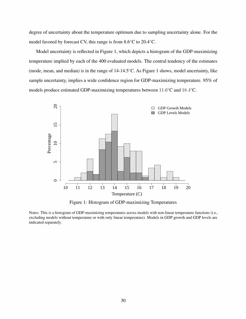
Model uncertainty is reflected in Figure 1, which depicts a histogram of the GDP-maximizing

temperature implied by each of the 400 evaluated models. The central tendency of the estimates

(mode, mean, and median) is in the range of 14-14.5◦C. As Figure 1 shows, model uncertainty, like

sample uncertainty, implies a wide confidence region for GDP-maximizing temperature. 95% of

models produce estimated GDP-maximizing temperatures between 11.6◦C and 18.4◦C.

Temperature (C)

Per

cent

age

05

1015

20

10 11 12 13 14 15 16 17 18 19 20

GDP Growth ModelsGDP Levels Models

Figure 1: Histogram of GDP-maximizing Temperatures

Notes: This is a histogram of GDP-maximizing temperatures across models with non-linear temperature functions (i.e.,excluding models without temperature or with only linear temperature). Models in GDP growth and GDP levels areindicated separately.

30

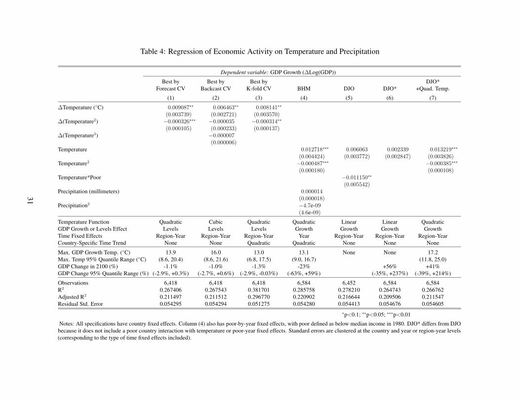
Table 4: Regression of Economic Activity on Temperature and Precipitation

Dependent variable: GDP Growth (∆Log(GDP))

Best by Best by Best by DJO*Forecast CV Backcast CV K-fold CV BHM DJO DJO* +Quad. Temp.

(1) (2) (3) (4) (5) (6) (7)

∆Temperature (◦C) 0.009087∗∗ 0.006463∗∗ 0.008141∗∗

(0.003739) (0.002721) (0.003570)∆(Temperature2) −0.000326∗∗∗ −0.000035 −0.000314∗∗

(0.000105) (0.000233) (0.000137)∆(Temperature3) −0.000007

(0.000006)Temperature 0.012718∗∗∗ 0.006063 0.002339 0.013219∗∗∗

(0.004424) (0.003772) (0.002847) (0.003826)Temperature2 −0.000487∗∗∗ −0.000385∗∗∗

(0.000180) (0.000108)Temperature*Poor −0.011150∗∗

(0.005542)Precipitation (millimeters) 0.000014

(0.000018)Precipitation2 −4.7e-09

(4.6e-09)

Temperature Function Quadratic Cubic Quadratic Quadratic Linear Linear QuadraticGDP Growth or Levels Effect Levels Levels Levels Growth Growth Growth GrowthTime Fixed Effects Region-Year Region-Year Region-Year Year Region-Year Region-Year Region-YearCountry-Specific Time Trend None None Quadratic Quadratic None None None

Max. GDP Growth Temp. (◦C) 13.9 16.0 13.0 13.1 None None 17.2Max. Temp 95% Quantile Range (◦C) (8.6, 20.4) (8.6, 21.6) (6.8, 17.5) (9.0, 16.7) (11.8, 25.0)GDP Change in 2100 (%) -1.1% -1.0% -1.3% -23% +56% +41%GDP Change 95% Quantile Range (%) (-2.9%, +0.3%) (-2.7%, +0.6%) (-2.9%, -0.03%) (-63%, +59%) (-35%, +237%) (-39%, +214%)

Observations 6,418 6,418 6,418 6,584 6,452 6,584 6,584R2 0.267406 0.267543 0.381701 0.285758 0.278210 0.264743 0.266762Adjusted R2 0.211497 0.211512 0.296770 0.220902 0.216644 0.209506 0.211547Residual Std. Error 0.054295 0.054294 0.051275 0.054280 0.054413 0.054676 0.054605

∗p<0.1; ∗∗p<0.05; ∗∗∗p<0.01

Notes: All specifications have country fixed effects. Column (4) also has poor-by-year fixed effects, with poor defined as below median income in 1980. DJO* differs from DJObecause it does not include a poor country interaction with temperature or poor-year fixed effects. Standard errors are clustered at the country and year or region-year levels(corresponding to the type of time fixed effects included).

31

4.3 Estimated GDP Impact of Climate Change

As described in section 3.4, the parameter estimates from the econometric models of DJO, BHM,

and the 399 variants are used to project economic impacts of unmitigated warming. As in BHM,

we project the impact of expected warming on global GDP by 2100 using the RCP8.5 climate

projection as a benchmark of unmitigated climate change and SSP5 for projections of baseline

GDP and population growth. In addition to examining the variation in GDP impacts due to model

uncertainty, we evaluate sampling uncertainty using a bootstrap procedure for the subset of models

appearing in any MCS and including non-linear temperature functions. We are, thus, able to relate

sampling uncertainty to model uncertainty and assess the variance in projected GDP losses due to

both.

Figure 2 shows the estimated percentage changes in GDP in 2100 under the RCP8.5 scenario

for all models that include temperature. It plots the histogram of damage estimates from 160 GDP

growth models (top panel) and 160 GDP levels models (bottom panel, note the different scale of the

x-axis). In each panel, damages from models featuring linear and non-linear temperature functions

are distinguished. Table 5 shows the estimated damages for each model that incorporates a quadratic

of precipitation. A corresponding table in the appendix shows these estimates for models that

exclude precipitation. Among these are the models that perform best in CV (see Appendix Table

A5).38

As evidenced in Figure 2 and Table 5, the evaluated models project a wide range of global GDP

impacts in 2100. The large variation in estimated GDP impacts across models is due primarily to

the importance of the GDP-maximizing temperature level relative to the location of the world’s

major economies. Small shifts in the GDP-maximizing temperature can change whether GDP of a

few major economies would benefit from or be harmed by projected warming under this estimation

approach. Across all models, GDP impacts range from -48% to +157%. This variation is attributed

38GDP impact estimates for models that incorporate other precipitation functions (linear, cubic, spline) are similar.The GDP impacts for models that exclude temperature are not reported because they are zero by construction.

32

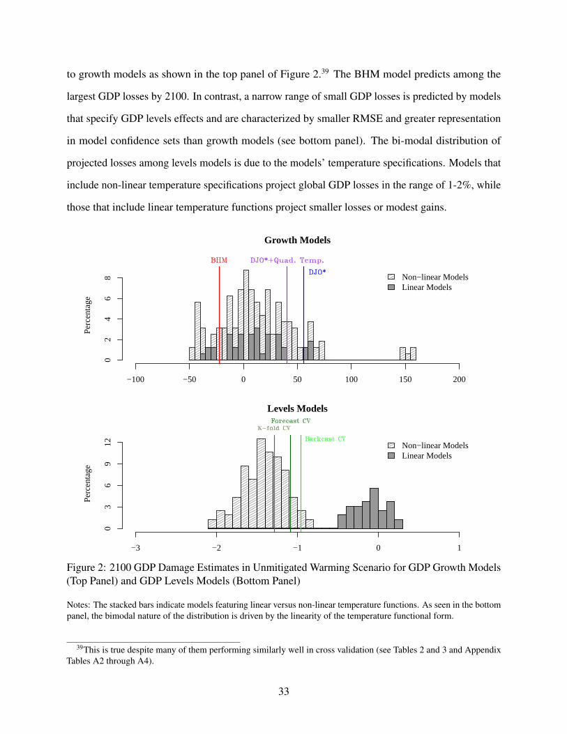
to growth models as shown in the top panel of Figure 2.39 The BHM model predicts among the

largest GDP losses by 2100. In contrast, a narrow range of small GDP losses is predicted by models

that specify GDP levels effects and are characterized by smaller RMSE and greater representation

in model confidence sets than growth models (see bottom panel). The bi-modal distribution of

projected losses among levels models is due to the models’ temperature specifications. Models that

include non-linear temperature specifications project global GDP losses in the range of 1-2%, while

those that include linear temperature functions project smaller losses or modest gains.

Per

cent

age

−100 −50 0 50 100 150 200

02

46

8 Non−linear ModelsLinear Models

Growth Models

Per

cent

age

−3 −2 −1 0 1

Non−linear ModelsLinear Models

03

69

12

Levels Models

Figure 2: 2100 GDP Damage Estimates in Unmitigated Warming Scenario for GDP Growth Models(Top Panel) and GDP Levels Models (Bottom Panel)

Notes: The stacked bars indicate models featuring linear versus non-linear temperature functions. As seen in the bottompanel, the bimodal nature of the distribution is driven by the linearity of the temperature functional form.

39This is true despite many of them performing similarly well in cross validation (see Tables 2 and 3 and AppendixTables A2 through A4).

33

GDP Growth Effects Models. GDP losses are highly sensitive to modest changes in modeling

assumptions of growth models, as shown in the top panels of Tables 5 and A5. Models that include

year fixed effects and a quadratic or higher-order time trend almost always imply GDP losses.

In contrast, models that exclude the parametric time trend universally imply GDP gains from

warming by 2100 whether year or region-year fixed effects are included. The DJO-adapted model

(DJO∗), for instance, implies GDP gains of 56% by 2100. Modest changes to the specifications

of BHM amd DJO generate large changes in GDP impact predictions. Simply adding a cubic

temperature term to BHM’s specification reduces the estimated GDP impacts by half (-11% versus

-23%). Removing BHM’s country-specific time trends reverses the sign of the impacts (+12%)

and using region-year fixed effects also reverses the sign (+10%). Starting with DJO’s model and

adding quadratic temperature reverses the sign of impacts (+41%). The set of statistically superior

temperature-growth models in forecast CV imply GDP gains of +41% to +157%. The superior set

in backcast CV implies GDP gains of −1 to +157%.

GDP Level Effects Models. Nearly all levels-effect models imply GDP losses of 2% or less, as

reported in the bottom panels of Tables 5 and A5.40 Only 4 of the 64 levels-effect models shown

in Tables 5 and A5 (and only 12 of all 160 levels models) project GDP gains, all of which assume

linear temperature effects. The remaining levels-effect models project losses of about 1-2% of GDP,

including the models that minimize prediction error (RMSE) across CV methods. The largest loss

projected by a GDP levels model is 2.0%.

Sampling and Modeling Uncertainty. Model and sampling uncertainty are separately compared

for growth and levels models by considering temperature parameter estimates from bootstrapped

samples for each model that appears in an MCS and incorporates non-linear temperature functions.41

Bootstrap samples are drawn 1,000 times for each model and are block-sampled by country. Each

40A regional disaggregation of these global impacts does not show substantially different impacts on any particularcountry, with India accounting for the single biggest loss.

41Theory and micro-foundations suggest a preference for non-linear temperature functions even though these modelsdo not perform better in cross validation than models with linear temperature functions. By assessing uncertainty amongonly models with non-linear temperature functions, we constrain model uncertainty, which is nevertheless shown to beimmense.

34

set of temperature parameter estimates is used to project GDP losses in 2100, yielding a distribution

of predicted global GDP impacts for each model in the union of model confidence sets.

These distributions are depicted in Figure 3. The top panel shows distributions of 60 growth

models, and the bottom panel shows distributions of 73 levels models (note different scales of

horizontal axes). Distributions in the bottom panel highlighted in green are those of the models that

perform best in CV. The violet distribution in the top panel is that of ”DJO*+Quad. Temp.” Bolded

blue curves in each panel depict the distributions of GDP impacts across all bootstrap samples and

all models.

The top panel in Figure 3 demonstrates considerable sampling uncertainty for models in GDP

growth; individual model distributions range from 80-100% losses to greater than 500% gains for

some models.42 Across models, the distribution of impacts is centered at gains of +28% (median)

to +55% (mean), though some models, like that of BHM, are centered at losses of 20-30% and

still others are massed at GDP gains of +60%. Whereas BHM acknowledge a 30% chance that

future warming under RCP8.5 yields GDP gains, this likelihood is greater when accounting for

model and sampling uncertainty. Sixty-six percent of the mass of the pooled distribution is above

zero. The 95 percentile range across models and samples is -56% to +340%. Sampling uncertainty

is characterized by the average variance of GDP impact estimates holding models constant and

varying samples. It can be related to the magnitude of model uncertainty, characterized by average

variance of impact estimates as models vary and samples are held constant. The combined variance

is the variance across all impact estimates as is shown in the blue curve of the top panel. Model

uncertainty, as measured by the average standard deviation of GDP impacts across models, is equal

to 85% of GDP. It is larger than sampling uncertainty, which is equal to 63% of GDP. Combined

uncertainty is equal to 108% of GDP. The magnitude of combined uncertainty demonstrates the

challenge posed if one relies on econometric specifications of a temperature-growth relationship for

policy analysis.

42The x-axis in the top panel is truncated at +500% GDP impacts, but the tail extends as high at +1500%.

35

The bottom panel in Figure 3 shows less variation in predicted GDP impacts across bootstrap

samples and across models in GDP levels. For nearly all of the distributions depicted, GDP impacts

are centered around −1% to −2%. Ninety-five percent of the mass of the pooled distribution falls

in the interval (−3.1%,+0.2%). The frequency of impacts worse than −2% GDP is about 30%,

and there is only a 4% frequency of positive GDP impacts. Figure 3 also shows less uncertainty in

impacts than was found in the bootstrap exercise in BHM, which estimated a 30% probability of

positive GDP impacts (compared to a 4% probability found here). This is attributable to the smaller

magnitude and uncertainty of impacts from GDP levels models. Model uncertainty is equal to 0.8%

of GDP, whereas sample uncertainty is only half as large. Combined uncertainty is equal to 0.84%

of GDP.

4.4 Temperature Impacts by Country Income and Sector

Rich vs. Poor Countries. BHM report that both poor and rich country GDP respond non-linearly

to temperature.43 This suggests climate change impacts are broader than those implied by DJO,

which found negative impacts only on poor countries. When we separately estimate parameters

for rich and poor countries, we find that temperature impacts are less statistically significant and

smaller in magnitude for rich countries.44 We only identify a consistent statistically significant

relationship between temperature and GDP growth for poor countries.45 As reported in the top panel

of Appendix Table A6, the models favored by CV do not imply statistically significant quadratic

temperature effects for rich countries. Nor does the BHM model. Though the coefficients on the

temperature terms are mostly statistically insignificant, they do imply the concave relationship

identified by BHM.46 Likewise, among poor countries, the quadratic temperature term is statistically

significant in two of the three the models favored by CV and marginally significant in the BHM43Deryugina and Hsiang (2014) also find significant temperature effects on U.S. GDP.44In a study focusing on productivity growth, Letta and Tol (2018) also find significant impacts of temperature on

poor countries but not rich ones.45DJO and BHM do not estimate heterogeneous effects on separate samples of rich and poor countries as we do.

Instead, they introduce interactions of temperature (and in some cases, year fixed effects or region-year fixed effects)with an indicator for “poor”, as shown in Appendix Table A7. Our approach admits greater heterogeneity, including inthe error structure.

46Standard errors on temperature-squared terms are slightly larger in the rich sample regression than in the pooledsample regression, reflecting some loss in precision. Were the precision of the pooled sample regression retained,

36

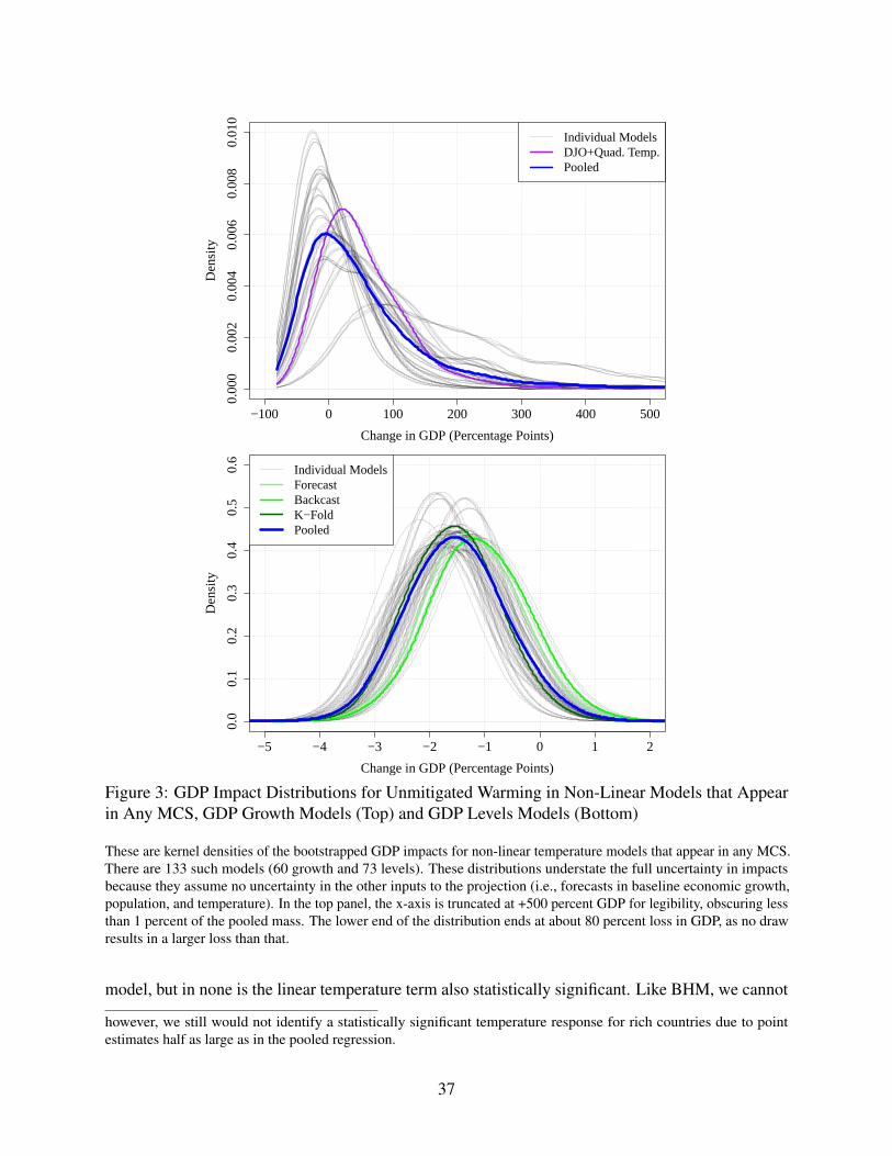
0.00

00.

002

0.00

40.

006

0.00

80.

010

Change in GDP (Percentage Points)

Den

sity

−100 0 100 200 300 400 500

Individual ModelsDJO+Quad. Temp.Pooled

0.0

0.1

0.2

0.3

0.4

0.5

0.6

Change in GDP (Percentage Points)

Den

sity

−5 −4 −3 −2 −1 0 1 2

Individual ModelsForecastBackcastK−FoldPooled

Figure 3: GDP Impact Distributions for Unmitigated Warming in Non-Linear Models that Appearin Any MCS, GDP Growth Models (Top) and GDP Levels Models (Bottom)

These are kernel densities of the bootstrapped GDP impacts for non-linear temperature models that appear in any MCS.There are 133 such models (60 growth and 73 levels). These distributions understate the full uncertainty in impactsbecause they assume no uncertainty in the other inputs to the projection (i.e., forecasts in baseline economic growth,population, and temperature). In the top panel, the x-axis is truncated at +500 percent GDP for legibility, obscuring lessthan 1 percent of the pooled mass. The lower end of the distribution ends at about 80 percent loss in GDP, as no drawresults in a larger loss than that.

model, but in none is the linear temperature term also statistically significant. Like BHM, we cannot

however, we still would not identify a statistically significant temperature response for rich countries due to pointestimates half as large as in the pooled regression.

37

reject the hypothesis that marginal temperature effects are common across rich and poor countries

for all average annual temperatures in our data.

Agriculture vs. Non-Agriculture Sectors. BHM and DJO also conclude that non-agricultural

production growth is affected by temperature shocks. When rich and poor countries are pooled but

agricultural and non-agricultural GDP are disaggregated, the statistical significance of temperature

impacts is diminished in models preferred by CV (Appendix Table A8). Nevertheless, coefficients

for non-agricultural output are similar to those of aggregate GDP, and agricultural output responses

are more concave. Disaggregating further by rich (Appendix Table A9) and poor (Appendix Table

A10) countries, we do not identify a statistically significant temperature effect on rich country

agricultural or non-agricultural output using the models favored by CV or by BHM. Likewise, the

models favored by forecast and backcast CV do not identify a statistically significant temperature

effect on non-agricultural production in poor countries. The magnitude of the temperature coeffi-

cients vary across these models, leading to significant variation in the implied output-maximizing

temperature.

5 Conclusion

In the absence of clear theoretical guidance on specific estimable forms for the aggregate GDP-

temperature relationship, we consider the implications of model uncertainty for market damages

of climate change. Out-of-sample predictive accuracy is assessed for 400 variants of prominent

models that vary by specification of the temperature functions, controls for unobserved trends, and

the dependent variable. Cross validation is employed to determine model prediction errors, which

are used to determine the sets of models that have statistically significant superior performance.

The best performing models are those that relate temperature to GDP levels rather than GDP

growth. Though we cannot preclude at 95% confidence that a model relating temperature to GDP

growth is superior, we conclude with 95% confidence that the model preferred by Burke et al.

(2015) is not among the superior models. Growth models generate considerably greater uncertainty

38

of climate impacts than do levels models. For growth models with superior but statistically

indistinguishable performance, the 95% confidence region of GDP impacts in 2100 is -56% to

+340%, including both model and sampling uncertainty. Modeling uncertainty, uniquely estimated

in this paper, is shown to be larger than sampling uncertainty. Models relating temperature to GDP

levels estimate climate impacts with far less uncertainty. The best models imply GDP losses by

2100 of 1-2%. A 95% confidence region is from -3.1% to +0.2%.

Given the considerable sample and model uncertainty associated with growth models, their

usefulness in policy analysis is not obvious. In so far as theory or other information equips the

modeler with reason to prefer models relating temperature to GDP levels and not growth, then the

econometric approach to estimating aggregate GDP impacts generates information that can inform

integrated assessment models, the social cost of carbon, and climate policy in general. Results from

the best of these models are consistent with damage functions currently embedded in the major

integrated assessment models that underpin the U.S. social cost of carbon (National Academies of

Sciences 2017; Nordhaus 2017; Rose et al. 2017; National Research Council 2010). While these

impacts may appear modest, even a 1% loss to global GDP is equal to $800 billion today and could

be 5-12 times greater by 2100 assuming 2-3% annual economic growth. Moreover, projected GDP

impacts based on past temperature fluctuations reflect only a component of potential welfare effects,

excluding, for instance, effects on non-market goods like environmental amenities and potential

extreme events not reflected in the historical record.

ReferencesACEMOGLU, D., JOHNSON, S. and ROBINSON, J. A. (2002). Reversal of fortune: Geography and

institutions in the making of the modern world income distribution. The Quarterly Journal ofEconomics, 117 (4), 1231–1294.

ANTTILA-HUGHES, J. K. and HSIANG, S. M. (2011). Destruction, disinvestment, and death:Economic and human losses following environmental disaster.

ARLOT, S. and CELISSE, A. (2010). A survey of cross-validation procedures for model selection.Statistics surveys, 4, 40–79.

39

ATHEY, S. (2017). The impact of machine learning on economics. In Economics of ArtificialIntelligence, University of Chicago Press.

AUFFHAMMER, M. and STEINHAUSER, R. (2012). Forecasting the path of U.S. CO2 emissionsusing state-level information. Review of Economics and Statistics, 94 (1), 172–185.

BARRIOS, S., BERTINELLI, L. and STROBL, E. (2010). Trends in Rainfall and Economic Growthin Africa: A Neglected Cause of the African Growth Tragedy. Review of Economics and Statistics,92 (2), 350–366.

BELLONI, A., CHERNOZHUKOV, V. and HANSEN, C. (2014). Inference on treatment effects afterselection among high-dimensional controls. The Review of Economic Studies, 81 (2), 608–650.

BERNANKE, B. S. and GURKAYNAK, R. S. (2001). Is Growth Exogenous? Taking Mankiw,Romer, and Weil Seriously. NBER Macroeconomics Annual, 16, 11–57.

BURKE, M., DAVIS, W. M. and DIFFENBAUGH, N. S. (2018). Large potential reduction ineconomic damages under UN mitigation targets. Nature, 557 (7706), 549.

— and EMERICK, K. (2015). Adaptation to climate change: Evidence from U.S. agriculture.Working Paper.

—, HSIANG, S. M. and MIGUEL, E. (2015). Global non-linear effect of temperature on economicproduction. Nature, 527 (7577), 235–239.

CACHON, G. P., GALLINO, S. and OLIVARES, M. (2012). Severe weather and automobile assemblyproductivity. Columbia Business School Research Paper, (12/37).

CARLETON, T. A. and HSIANG, S. M. (2016). Social and economic impacts of climate. Science,353 (6304), aad9837.

CHATFIELD, C. (1996). Model uncertainty and forecast accuracy. Journal of Forecasting, 15 (7),495–508.

CHRISTENSEN, G. and MIGUEL, E. (Forthcoming). Transparency, reproducibility, and the credibil-ity of economics research. Journal of Economic Literature.

COOLEY, T. F. and LEROY, S. F. (1981). Identification and estimation of money demand. TheAmerican Economic Review, 71 (5), 825–844.

DELL, M., JONES, B. F. and OLKEN, B. A. (2012). Temperature shocks and economic growth:Evidence from the last half century. American Economic Journal: Macroeconomics, 4 (3), 66–95.

—, — and — (2014). What do we learn from the weather? The new climate–economy literature.Journal of Economic Literature, 52 (3), 740–798.

DERYUGINA, T. (2011). The dynamic effects of hurricanes in the U.S.: The role of non-disastertransfer payments. MIT Center for Energy and Environmental Policy Research, Working Paper.

40

— and HSIANG, S. M. (2014). Does the Environment Still Matter? Daily Temperature and Incomein the United States. NBER Working Paper No. 20750.

DESCHENES, O. and GREENSTONE, M. (2007). The economic impacts of climate change: Ev-idence from agricultural output and random fluctuations in weather. The American EconomicReview, 97 (1), 354–385.

DESCHENES, O. and GREENSTONE, M. (2012). The economic impacts of climate change: Evi-dence from agricultural output and random fluctuations in weather: Reply. American EconomicReview, 102 (7), 3761–3773.

DHRYMES, P. J., HOWREY, E. P., HYMANS, S. H., KMENTA, J., LEAMER, E. E., QUANDT,R. E., RAMSEY, J. B., SHAPIRO, H. T. and ZARNOWITZ, V. (1972). Criteria for evaluationof econometric models. In Annals of Economic and Social Measurement, Volume 1, number 3,NBER, pp. 291–324.

DIEBOLD, F. X. and MARIANO, R. S. (1995). Comparing predictive accuracy. Journal of Business& Economic Statistics, 13 (3), 253–263.

EASTERLY, W. and LEVINE, R. (2003). Tropics, germs, and crops: How endowments influenceeconomic development. Journal of Monetary Economics, 50 (1), 3–39.

FANKHAUSER, S. (1994). The social costs of greenhouse gas emissions: An expected valueapproach. The Energy Journal, pp. 157–184.

— (2013). Valuing climate change: The economics of the greenhouse. London: Routledge.

FENG, S., KRUEGER, A. B. and OPPENHEIMER, M. (2010). Linkages among climate change, cropyields and Mexico-US cross-border migration. Proceedings of the National Academy of Sciences,107 (32), 14257–14262.

FISHER, A. C., HANEMANN, W. M., ROBERTS, M. J. and SCHLENKER, W. (2012). The economicimpacts of climate change: Evidence from agricultural output and random fluctuations in weather:Comment. American Economic Review, 102 (7), 3749–3760.

FRIEDMAN, M. (1953). The methodology of positive economics. In Essays in Positive Economics,University of Chicago Press, pp. 3–16.

GEISSER, S. (1975). The predictive sample reuse method with applications. Journal of the Americanstatistical Association, 70 (350), 320–328.

GRAFF ZIVIN, J. and NEIDELL, M. (2014). Temperature and the allocation of time: Implicationsfor climate change. Journal of Labor Economics, 32 (1), 1–26.

GREEN, W. H. (2012). Econometric Analysis. Boston: Prentice Hall.

GREENSTONE, M., KOPITS, E. and WOLVERTON, A. (2013). Developing a social cost of carbonfor us regulatory analysis: A methodology and interpretation. Review of Environmental Economicsand Policy, 7 (1), 23–46.

41

HANSEN, P. R. (2005). A test for superior predictive ability. Journal of Business & EconomicStatistics, 23 (4), 365–380.

—, LUNDE, A. and NASON, J. M. (2011). The model confidence set. Econometrica, 79 (2),453–497.

HENDRY, D. F. (1980). Econometrics-alchemy or science? Economica, pp. 387–406.

—, LEAMER, E. E. and POIRIER, D. J. (1990). A conversation on econometric methodology.Econometric Theory, 6 (2), 171–261.

HSIANG, S. (2016). Climate econometrics. Annual Review of Resource Economics, 8 (1), 43–75.

HSIANG, S. M. (2010). Temperatures and cyclones strongly associated with economic production inthe Caribbean and Central America. Proceedings of the National Academy of Sciences, 107 (35),15367–15372.

— and JINA, A. S. (2014). The causal effect of environmental catastrophe on long-run economicgrowth: Evidence from 6,700 cyclones. NBER Working Paper No. 20352.

— and NARITA, D. (2012). Adaptation to cyclone risk: Evidence from the global cross-section.Climate Change Economics, 3 (2), 1250011.

JONES, B. F. and OLKEN, B. A. (2010). Climate shocks and exports. The American EconomicReview, 100 (2), 454–459.

KAHN, M. E. (2005). The death toll from natural disasters: The role of income, geography, andinstitutions. Review of Economics and Statistics, 87 (2), 271–284.

KAUFMANN, R. K., KAUPPI, H. and STOCK, J. H. (2010). Does temperature contain a stochastictrend? Evaluating conflicting statistical results. Climatic Change, 101 (3-4), 395–405.

KEYNES, J. M. (1939). Professor Tinbergen’s method. The Economic Journal, 49 (5), 559–577.

KLEINBERG, J., LUDWIG, J., MULLAINATHAN, S. and OBERMEYER, Z. (2015). Prediction policyproblems. American Economic Review, 105 (5), 491–95.

KOOPMANS, T. C. (1947). Measurement without theory. The Review of Economics and Statistics,29 (3), 161–172.

KOPITS, E., MARTEN, A. and WOLVERTON, A. (2014). Incorporating catastrophic climate changeinto policy analysis. Climate Policy, 14 (5), 637–664.

LEAMER, E. E. (1978). Specification searches: Ad hoc inference with nonexperimental data, vol. 53.John Wiley & Sons Incorporated.

— (1983). Let’s take the con out of econometrics. The American Economic Review, 73 (1), 31–43.

— (2010). Tantalus on the road to asymptopia. Journal of Economic Perspectives, 24 (2), 31–46.

42

LETTA, M. and TOL, R. S. J. (2018). Weather, climate and total factor productivity. Environmentaland Resource Economics, pp. 1–23.

LOBELL, D. B., SCHLENKER, W. and COSTA-ROBERTS, J. (2011). Climate trends and globalcrop production since 1980. Science, 333 (6042), 616–620.

MADDISON, D. (2003). The amenity value of the climate: The household production functionapproach. Resource and Energy Economics, 25 (2), 155–175.

MANKIW, N. G., ROMER, D. and WEIL, D. N. (1992). A contribution to the empirics of economicgrowth. The Quarterly Journal of Economics, 107 (2), 407–437.

MATSUURA, K. and WILLMOTT, C. J. (2012). Terrestrial air temperature and precipitation:Monthly and annual time series (1900 - 2010) v 3.01. Available at http://climate.geog.udel.edu/˜climate/html_pages/download.html#T2011.

MCINTOSH, C. T. and SCHLENKER, W. (2006). Identifying non-linearities in fixed effects models.UC-San Diego Working Paper.

MENDELSOHN, R., MORRISON, W., SCHLESINGER, M. E. and ANDRONOVA, N. G. (2000a).Country-specific market impacts of climate change. Climatic Change, 45 (3-4), 553–569.

—, NORDHAUS, W. D. and SHAW, D. (1994). The impact of global warming on agriculture: ARicardian analysis. The American Economic Review, pp. 753–771.

—, SCHLESINGER, M. and WILLIAMS, L. (2000b). Comparing impacts across climate models.Integrated Assessment, 1 (1), 37–48.

MOORE, F. C. and DIAZ, D. B. (2015). Temperature impacts on economic growth warrant stringentmitigation policy. Nature Climate Change, 5 (2), 127–131.

NATIONAL ACADEMIES OF SCIENCES (2017). Valuing climate damages: Updating estimation ofthe social cost of carbon dioxide. National Academies Press.

NATIONAL RESEARCH COUNCIL (2010). Hidden Costs of Energy: Unpriced Consequences ofEnergy Production and Use. National Academies Press.

NORDHAUS, W. D. (1994). Managing the Global Commons: The Economics of Climate Change,vol. 31. Cambridge, MA: MIT Press.

— (2006). Geography and macroeconomics: New data and new findings. Proceedings of theNational Academy of Sciences of the United States of America, 103 (10), 3510–3517.

— (2008). A Question of Balance: Weighing the Options on Global Warming Policies. New Haven:Yale University Press.

— (2017). Revisiting the social cost of carbon. Proceedings of the National Academy of Sciences,114 (7), 1518–1523.

43

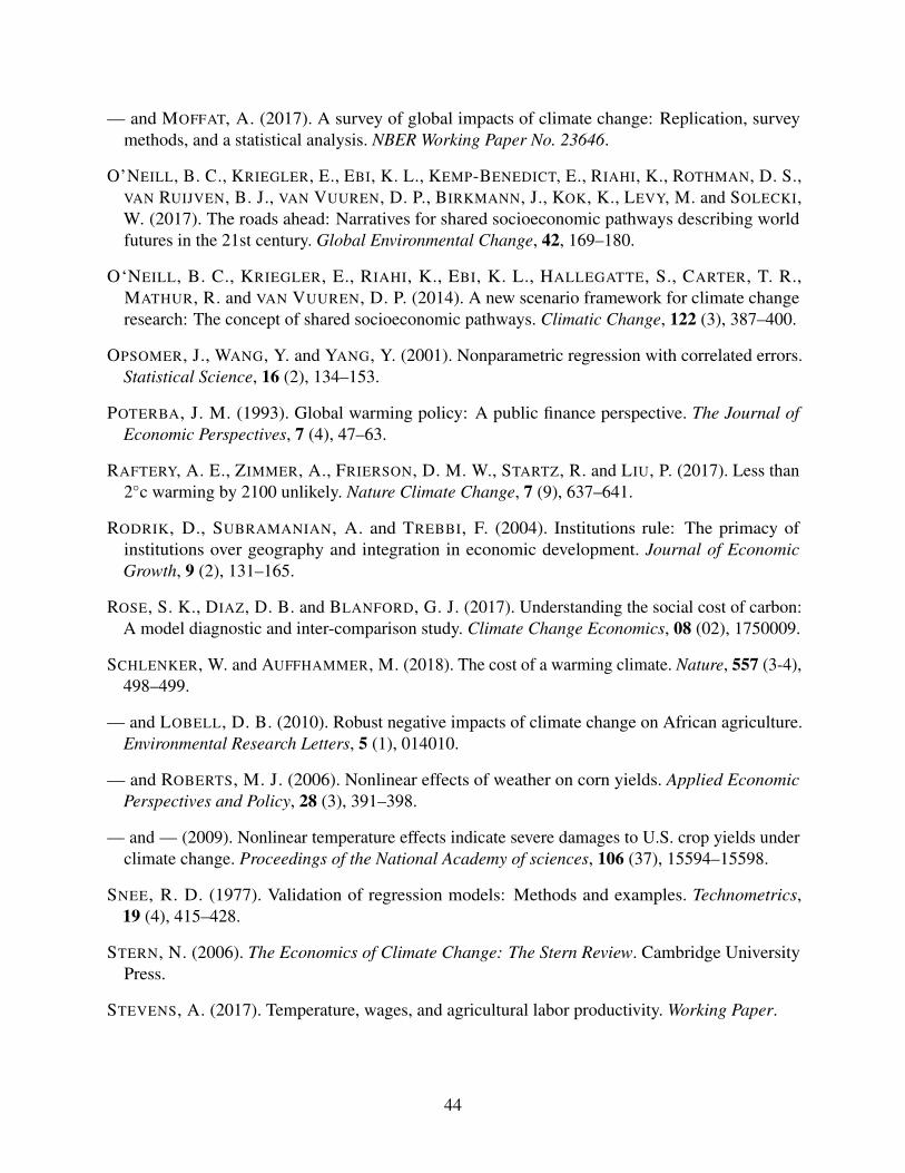
http://climate.geog.udel.edu/~climate/html_pages/download.html#T2011

http://climate.geog.udel.edu/~climate/html_pages/download.html#T2011

— and MOFFAT, A. (2017). A survey of global impacts of climate change: Replication, surveymethods, and a statistical analysis. NBER Working Paper No. 23646.

O’NEILL, B. C., KRIEGLER, E., EBI, K. L., KEMP-BENEDICT, E., RIAHI, K., ROTHMAN, D. S.,VAN RUIJVEN, B. J., VAN VUUREN, D. P., BIRKMANN, J., KOK, K., LEVY, M. and SOLECKI,W. (2017). The roads ahead: Narratives for shared socioeconomic pathways describing worldfutures in the 21st century. Global Environmental Change, 42, 169–180.

O‘NEILL, B. C., KRIEGLER, E., RIAHI, K., EBI, K. L., HALLEGATTE, S., CARTER, T. R.,MATHUR, R. and VAN VUUREN, D. P. (2014). A new scenario framework for climate changeresearch: The concept of shared socioeconomic pathways. Climatic Change, 122 (3), 387–400.

OPSOMER, J., WANG, Y. and YANG, Y. (2001). Nonparametric regression with correlated errors.Statistical Science, 16 (2), 134–153.

POTERBA, J. M. (1993). Global warming policy: A public finance perspective. The Journal ofEconomic Perspectives, 7 (4), 47–63.

RAFTERY, A. E., ZIMMER, A., FRIERSON, D. M. W., STARTZ, R. and LIU, P. (2017). Less than2◦c warming by 2100 unlikely. Nature Climate Change, 7 (9), 637–641.

RODRIK, D., SUBRAMANIAN, A. and TREBBI, F. (2004). Institutions rule: The primacy ofinstitutions over geography and integration in economic development. Journal of EconomicGrowth, 9 (2), 131–165.

ROSE, S. K., DIAZ, D. B. and BLANFORD, G. J. (2017). Understanding the social cost of carbon:A model diagnostic and inter-comparison study. Climate Change Economics, 08 (02), 1750009.

SCHLENKER, W. and AUFFHAMMER, M. (2018). The cost of a warming climate. Nature, 557 (3-4),498–499.

— and LOBELL, D. B. (2010). Robust negative impacts of climate change on African agriculture.Environmental Research Letters, 5 (1), 014010.

— and ROBERTS, M. J. (2006). Nonlinear effects of weather on corn yields. Applied EconomicPerspectives and Policy, 28 (3), 391–398.

— and — (2009). Nonlinear temperature effects indicate severe damages to U.S. crop yields underclimate change. Proceedings of the National Academy of sciences, 106 (37), 15594–15598.

SNEE, R. D. (1977). Validation of regression models: Methods and examples. Technometrics,19 (4), 415–428.

STERN, N. (2006). The Economics of Climate Change: The Stern Review. Cambridge UniversityPress.

STEVENS, A. (2017). Temperature, wages, and agricultural labor productivity. Working Paper.

44

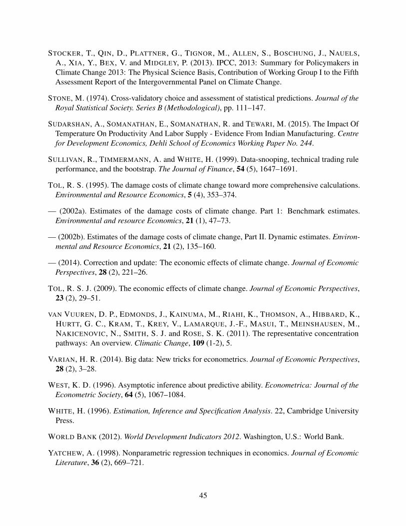
STOCKER, T., QIN, D., PLATTNER, G., TIGNOR, M., ALLEN, S., BOSCHUNG, J., NAUELS,A., XIA, Y., BEX, V. and MIDGLEY, P. (2013). IPCC, 2013: Summary for Policymakers inClimate Change 2013: The Physical Science Basis, Contribution of Working Group I to the FifthAssessment Report of the Intergovernmental Panel on Climate Change.

STONE, M. (1974). Cross-validatory choice and assessment of statistical predictions. Journal of theRoyal Statistical Society. Series B (Methodological), pp. 111–147.

SUDARSHAN, A., SOMANATHAN, E., SOMANATHAN, R. and TEWARI, M. (2015). The Impact OfTemperature On Productivity And Labor Supply - Evidence From Indian Manufacturing. Centrefor Development Economics, Dehli School of Economics Working Paper No. 244.

SULLIVAN, R., TIMMERMANN, A. and WHITE, H. (1999). Data-snooping, technical trading ruleperformance, and the bootstrap. The Journal of Finance, 54 (5), 1647–1691.

TOL, R. S. (1995). The damage costs of climate change toward more comprehensive calculations.Environmental and Resource Economics, 5 (4), 353–374.

— (2002a). Estimates of the damage costs of climate change. Part 1: Benchmark estimates.Environmental and resource Economics, 21 (1), 47–73.

— (2002b). Estimates of the damage costs of climate change, Part II. Dynamic estimates. Environ-mental and Resource Economics, 21 (2), 135–160.

— (2014). Correction and update: The economic effects of climate change. Journal of EconomicPerspectives, 28 (2), 221–26.

TOL, R. S. J. (2009). The economic effects of climate change. Journal of Economic Perspectives,23 (2), 29–51.

VAN VUUREN, D. P., EDMONDS, J., KAINUMA, M., RIAHI, K., THOMSON, A., HIBBARD, K.,HURTT, G. C., KRAM, T., KREY, V., LAMARQUE, J.-F., MASUI, T., MEINSHAUSEN, M.,NAKICENOVIC, N., SMITH, S. J. and ROSE, S. K. (2011). The representative concentrationpathways: An overview. Climatic Change, 109 (1-2), 5.

VARIAN, H. R. (2014). Big data: New tricks for econometrics. Journal of Economic Perspectives,28 (2), 3–28.

WEST, K. D. (1996). Asymptotic inference about predictive ability. Econometrica: Journal of theEconometric Society, 64 (5), 1067–1084.

WHITE, H. (1996). Estimation, Inference and Specification Analysis. 22, Cambridge UniversityPress.

WORLD BANK (2012). World Development Indicators 2012. Washington, U.S.: World Bank.

YATCHEW, A. (1998). Nonparametric regression techniques in economics. Journal of EconomicLiterature, 36 (2), 669–721.

45

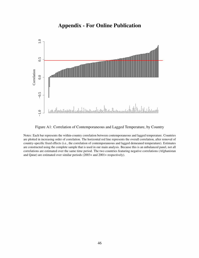
Appendix - For Online PublicationC

orre

latio

n

−1.

0−

0.5

0.0

0.5

1.0

Afg

hani

stan

Qat

arH

aiti

Vie

tnam

Arg

entin

aK

azak

hsta

nC

ambo

dia

Liby

aP

eru

Tha

iland

Lao

PD

RC

zech

Rep

ublic

Rus

sian

Fed

erat

ion

Slo

veni

aU

rugu

ayC

olom

bia

Aus

tral

iaC

anad

aK

orea

, Rep

.P

arag

uay

Tur

key

Pol

and

Yem

en, R

ep.

Gam

bia,

The

Kuw

ait

Lith

uani

aE

cuad

orE

ston

iaB

angl

ades

hH

unga

ryP

ortu

gal

Sou

th A

fric

aB

otsw

ana

Phi

lippi

nes

Japa

nS

ri La

nka

Pak

ista

nZ

imba

bwe

Syr

ian

Ara

b R

epub

licC

uba

Mol

dova

Indi

aS

erbi

aR

oman

iaN

amib

iaS

lova

k R

epub

licD

jibou

tiB

elar

usU

krai

neB

ulga

riaP

apua

New

Gui

nea

Aus

tria

Erit

rea

Mac

edon

ia, F

YR

Chi

leN

ew Z

eala

ndM

exic

oU

zbek

ista

nD

enm

ark

Sw

eden

Fin

land

Ang

ola

Moz

ambi

que

Mau

ritan

iaLa

tvia

Alb

ania

Om

anC

roat

iaA

rmen

iaIr

elan

dTa

nzan

iaG

erm

any

Bru

nei D

arus

sala

mB

oliv

iaS

witz

erla

ndB

huta

nM

ali

Mon

golia

Uni

ted

Sta

tes

Cab

o Ve

rde

Tajik

ista

nS

eneg

alS

waz

iland

Fiji

Cen

tral

Afr

ican

Rep

ublic

Uni

ted

Kin

gdom

Tur

kmen

ista

nLu

xem

bour

gG

reec

eN

orw

ayS

urin

ame

Net

herla

nds

Fra

nce

Jord

anIc

elan

dN

epal

Iran

, Isl

amic

Rep

.S

olom

on Is

land

sLe

soth

oG

eorg

iaC

hina

Leba

non

Pue

rto

Ric

oC

omor

osB

elgi

umIs

rael

Libe

riaZ

ambi

aS

pain

Gui

nea

Nig

erP

anam

aB

eliz

eC

ypru

sG

uyan

aG

hana

Con

go, R

ep.

Bra

zil

Mal

awi

Indo

nesi

aB

enin

Cot

e d'

Ivoi

reB

osni

a an

d H

erze

govi

naB

urki

na F

aso

Gre

enla

ndC

had

Mal

aysi

aE

gypt

, Ara

b R

ep.

Uni

ted

Ara

b E

mira

tes

Kyr

gyz

Rep

ublic

Mau

ritiu

sS

t. V

ince

nt a

nd th

e G

rena

dine

sIr

aqD

omin

ican

Rep

ublic

Vene

zuel

a, R

BM

oroc

coS

udan

Aze

rbai

jan

Ken

yaC

amer

oon

Sao

Tom

e an

d P

rinci

peTo

goG

uine

a−B

issa

uM

adag

asca

rC

ongo

, Dem

. Rep

.S

amoa

Nig

eria

Alg

eria

Bah

amas

, The

Italy

Eth

iopi

aT

rinid

ad a

nd T

obag

oS

ierr

a Le

one

Uga

nda

Bur

undi

Sau

di A

rabi

aT

unis

iaR

wan

daVa

nuat

uH

ondu

ras

Gab

onC

osta

Ric

aN

icar

agua

El S

alva

dor

Equ

ator

ial G

uine

aG

uate

mal

a

Figure A1: Correlation of Contemporaneous and Lagged Temperature, by Country

Notes: Each bar represents the within-country correlation between contemporaneous and lagged temperature. Countriesare plotted in increasing order of correlation. The horizontal red line represents the overall correlation, after removal ofcountry-specific fixed effects (i.e., the correlation of contemporaneous and lagged demeaned temperature). Estimatesare constructed using the complete sample that is used in our main analysis. Because this is an unbalanced panel, not allcorrelations are estimated over the same time period. The two countries featuring negative correlations (Afghanistanand Qatar) are estimated over similar periods (2003+ and 2001+ respectively).

46

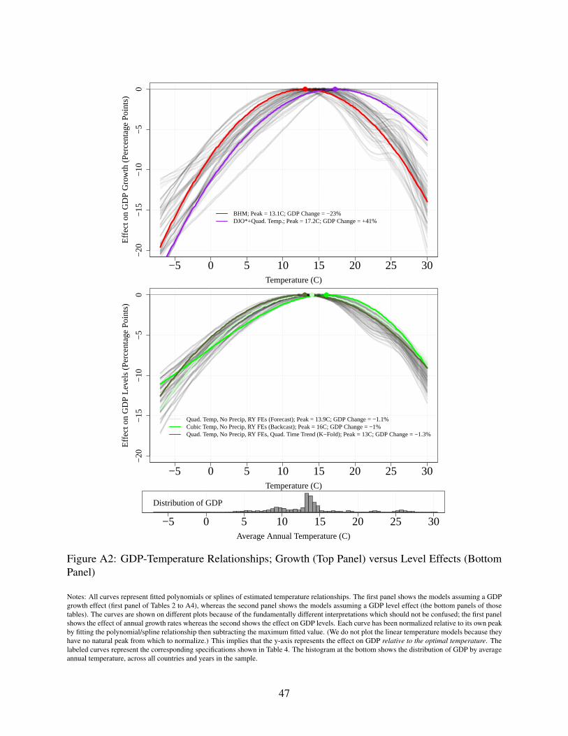
−20

−15

−10

−5

0

Temperature (C)

Effe

ct o

n G

DP

Gro

wth

(P

erce

ntag

e P

oint

s)

−5 0 5 10 15 20 25 30

●●

BHM; Peak = 13.1C; GDP Change = −23%DJO*+Quad. Temp.; Peak = 17.2C; GDP Change = +41%

−20

−15

−10

−5

0

Temperature (C)

Effe

ct o

n G

DP

Lev

els

(Per

cent

age

Poi

nts)

−5 0 5 10 15 20 25 30

● ●●

Quad. Temp, No Precip, RY FEs (Forecast); Peak = 13.9C; GDP Change = −1.1%Cubic Temp, No Precip, RY FEs (Backcast); Peak = 16C; GDP Change = −1%Quad. Temp, No Precip, RY FEs, Quad. Time Trend (K−Fold); Peak = 13C; GDP Change = −1.3%

Average Annual Temperature (C)

−5 0 5 10 15 20 25 30

Distribution of GDP

Figure A2: GDP-Temperature Relationships; Growth (Top Panel) versus Level Effects (BottomPanel)

Notes: All curves represent fitted polynomials or splines of estimated temperature relationships. The first panel shows the models assuming a GDPgrowth effect (first panel of Tables 2 to A4), whereas the second panel shows the models assuming a GDP level effect (the bottom panels of thosetables). The curves are shown on different plots because of the fundamentally different interpretations which should not be confused; the first panelshows the effect of annual growth rates whereas the second shows the effect on GDP levels. Each curve has been normalized relative to its own peakby fitting the polynomial/spline relationship then subtracting the maximum fitted value. (We do not plot the linear temperature models because theyhave no natural peak from which to normalize.) This implies that the y-axis represents the effect on GDP relative to the optimal temperature. Thelabeled curves represent the corresponding specifications shown in Table 4. The histogram at the bottom shows the distribution of GDP by averageannual temperature, across all countries and years in the sample.

47

The fitted relationships shown in Appendix Figure A2, graph the relationships implied by the

coefficient estimates in the non-linear temperature specifications considered.47). The top panel

of the figure plots fitted relationships corresponding to the models that specify a GDP growth

effect. The bottom panel depicts fitted curves for those models that specify a GDP level effect.

As previously discussed, these two effects are conceptually different on a fundamental level.

Despite this conceptual difference, the estimates generally suggest a concave relationship between

temperature and GDP, although the precise nature of that relationship varies.

The GDP-maximizing temperature ranges across models from 11◦C to 19◦C among growth

models and from 12◦C to 16◦C among levels models. Of these specifications, four of the models

considered in Table 4 are highlighted (the DJO models are not shown here because we have not

graphed models with only linear temperature). As previously seen in Table 4, the 13◦C peak of the

BHM model is a couple of degrees lower than the peaks of most other models in the first panel,

including DJO*+Quad. Temp. The two preferred models highlighted in green in the bottom panel

of Appendix Figure A2, also have peaks around 13◦C, but the curves are less concave.

47We do not depict models with only linear temperature because they have no natural “peak” at which to normalizethe figure, as is required and as we do in depicting the non-linear functions.

48

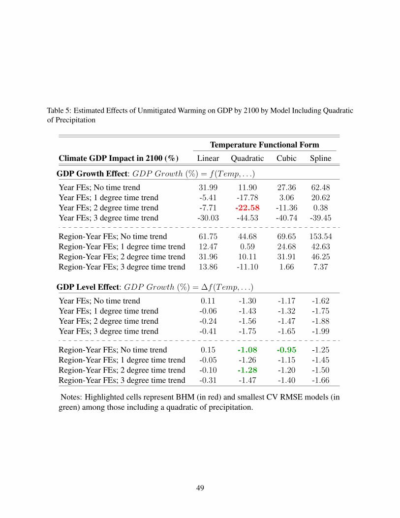
Table 5: Estimated Effects of Unmitigated Warming on GDP by 2100 by Model Including Quadraticof Precipitation

Temperature Functional FormClimate GDP Impact in 2100 (%) Linear Quadratic Cubic Spline


Year FEs; No time trend 31.99 11.90 27.36 62.48Year FEs; 1 degree time trend -5.41 -17.78 3.06 20.62Year FEs; 2 degree time trend -7.71 -22.58 -11.36 0.38Year FEs; 3 degree time trend -30.03 -44.53 -40.74 -39.45

Region-Year FEs; No time trend 61.75 44.68 69.65 153.54Region-Year FEs; 1 degree time trend 12.47 0.59 24.68 42.63Region-Year FEs; 2 degree time trend 31.96 10.11 31.91 46.25Region-Year FEs; 3 degree time trend 13.86 -11.10 1.66 7.37


Year FEs; No time trend 0.11 -1.30 -1.17 -1.62Year FEs; 1 degree time trend -0.06 -1.43 -1.32 -1.75Year FEs; 2 degree time trend -0.24 -1.56 -1.47 -1.88Year FEs; 3 degree time trend -0.41 -1.75 -1.65 -1.99

Region-Year FEs; No time trend 0.15 -1.08 -0.95 -1.25Region-Year FEs; 1 degree time trend -0.05 -1.26 -1.15 -1.45Region-Year FEs; 2 degree time trend -0.10 -1.28 -1.20 -1.50Region-Year FEs; 3 degree time trend -0.31 -1.47 -1.40 -1.66

Notes: Highlighted cells represent BHM (in red) and smallest CV RMSE models (ingreen) among those including a quadratic of precipitation.

49

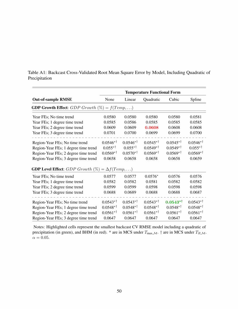
Table A1: Backcast Cross-Validated Root Mean Square Error by Model, Including Quadratic ofPrecipitation






Region-Year FEs; 1 degree time trend 0.055∗† 0.055∗† 0.0549∗† 0.0549∗† 0.055∗†


Region-Year FEs; 3 degree time trend 0.0658 0.0658 0.0658 0.0658 0.0659


Year FEs; No time trend 0.0577 0.0577 0.0576∗ 0.0576 0.0576Year FEs; 1 degree time trend 0.0582 0.0582 0.0581 0.0582 0.0582Year FEs; 2 degree time trend 0.0599 0.0599 0.0598 0.0598 0.0598Year FEs; 3 degree time trend 0.0688 0.0689 0.0688 0.0688 0.0687





Notes: Highlighted cells represent the smallest backcast CV RMSE model including a quadratic ofprecipitation (in green), and BHM (in red). * are in MCS under Tmax,M. † are in MCS under TR,M.α = 0.05.

50

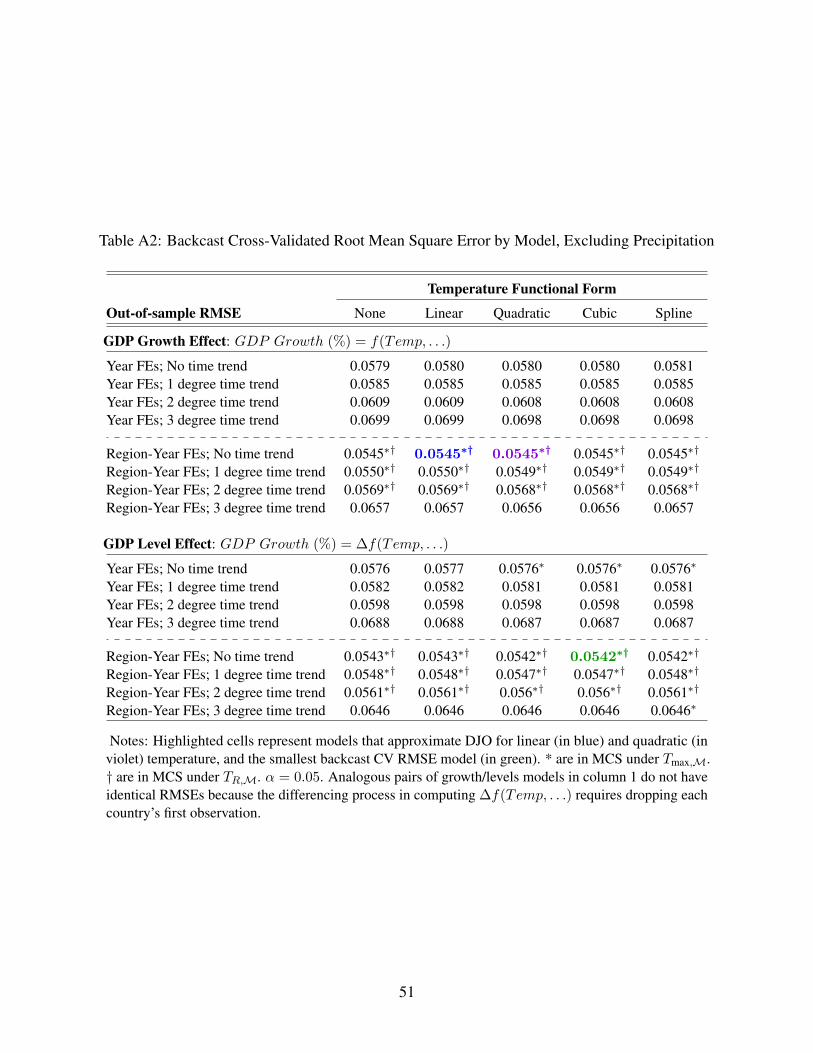
Table A2: Backcast Cross-Validated Root Mean Square Error by Model, Excluding Precipitation










Year FEs; No time trend 0.0576 0.0577 0.0576∗ 0.0576∗ 0.0576∗

Year FEs; 1 degree time trend 0.0582 0.0582 0.0581 0.0581 0.0581Year FEs; 2 degree time trend 0.0598 0.0598 0.0598 0.0598 0.0598Year FEs; 3 degree time trend 0.0688 0.0688 0.0687 0.0687 0.0687




Region-Year FEs; 3 degree time trend 0.0646 0.0646 0.0646 0.0646 0.0646∗

Notes: Highlighted cells represent models that approximate DJO for linear (in blue) and quadratic (inviolet) temperature, and the smallest backcast CV RMSE model (in green). * are in MCS under Tmax,M.† are in MCS under TR,M. α = 0.05. Analogous pairs of growth/levels models in column 1 do not haveidentical RMSEs because the differencing process in computing ∆f(Temp, . . .) requires dropping eachcountry’s first observation.

51

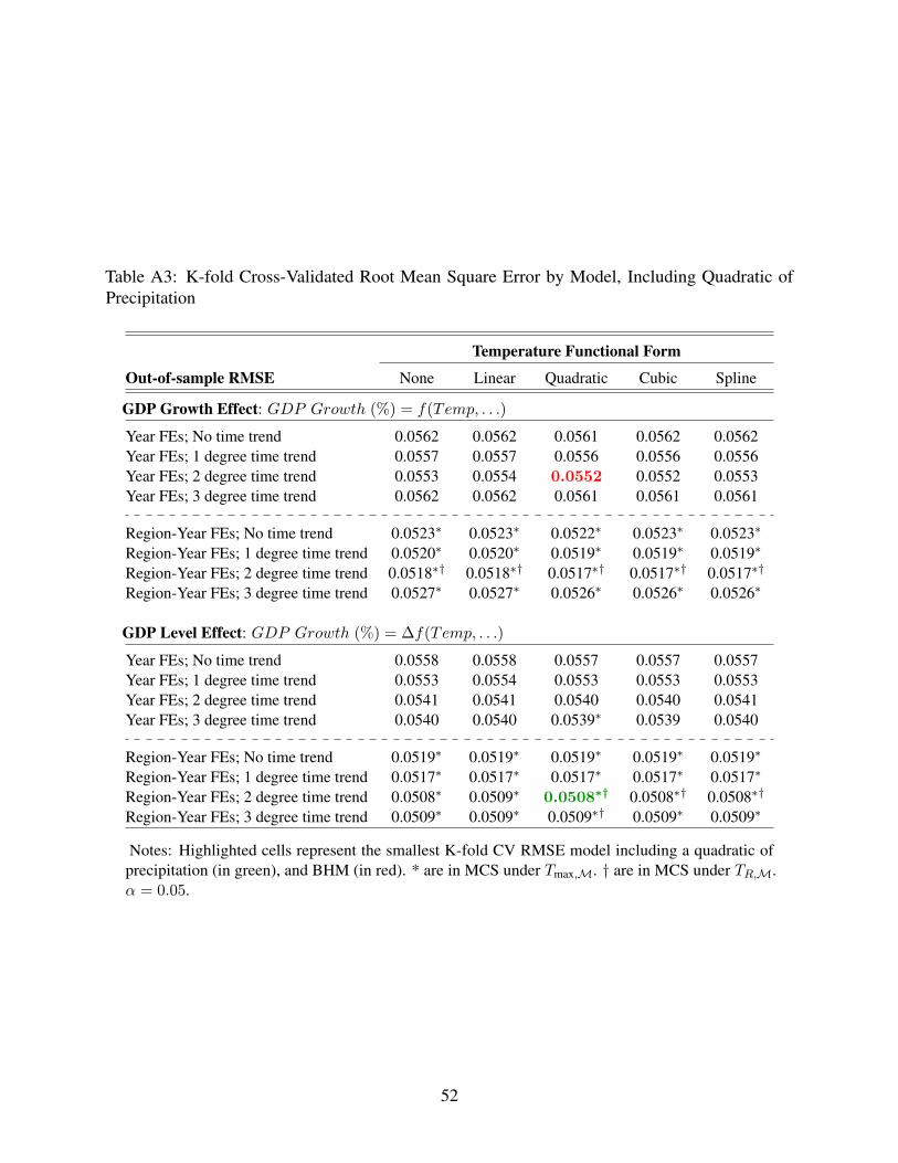
Table A3: K-fold Cross-Validated Root Mean Square Error by Model, Including Quadratic ofPrecipitation





Region-Year FEs; No time trend 0.0523∗ 0.0523∗ 0.0522∗ 0.0523∗ 0.0523∗

Region-Year FEs; 1 degree time trend 0.0520∗ 0.0520∗ 0.0519∗ 0.0519∗ 0.0519∗




Year FEs; No time trend 0.0558 0.0558 0.0557 0.0557 0.0557Year FEs; 1 degree time trend 0.0553 0.0554 0.0553 0.0553 0.0553Year FEs; 2 degree time trend 0.0541 0.0541 0.0540 0.0540 0.0541Year FEs; 3 degree time trend 0.0540 0.0540 0.0539∗ 0.0539 0.0540



Region-Year FEs; 2 degree time trend 0.0508∗ 0.0509∗ 0.0508∗† 0.0508∗† 0.0508∗†

Region-Year FEs; 3 degree time trend 0.0509∗ 0.0509∗ 0.0509∗† 0.0509∗ 0.0509∗

Notes: Highlighted cells represent the smallest K-fold CV RMSE model including a quadratic ofprecipitation (in green), and BHM (in red). * are in MCS under Tmax,M. † are in MCS under TR,M.α = 0.05.

52

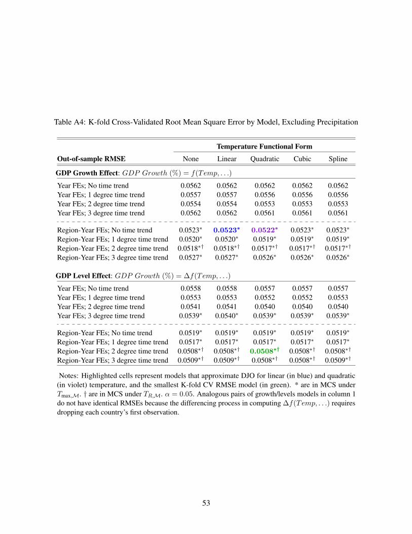
Table A4: K-fold Cross-Validated Root Mean Square Error by Model, Excluding Precipitation










Year FEs; No time trend 0.0558 0.0558 0.0557 0.0557 0.0557Year FEs; 1 degree time trend 0.0553 0.0553 0.0552 0.0552 0.0553Year FEs; 2 degree time trend 0.0541 0.0541 0.0540 0.0540 0.0540Year FEs; 3 degree time trend 0.0539∗ 0.0540∗ 0.0539∗ 0.0539∗ 0.0539∗





Notes: Highlighted cells represent models that approximate DJO for linear (in blue) and quadratic(in violet) temperature, and the smallest K-fold CV RMSE model (in green). * are in MCS underTmax,M. † are in MCS under TR,M. α = 0.05. Analogous pairs of growth/levels models in column 1do not have identical RMSEs because the differencing process in computing ∆f(Temp, . . .) requiresdropping each country’s first observation.

53

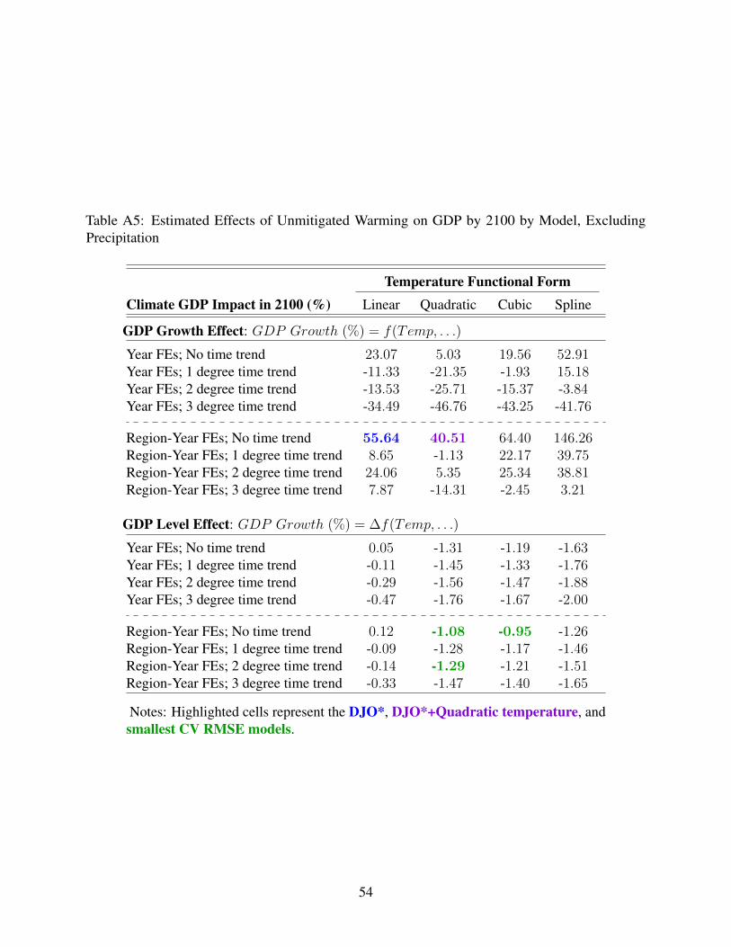
Table A5: Estimated Effects of Unmitigated Warming on GDP by 2100 by Model, ExcludingPrecipitation

Temperature Functional FormClimate GDP Impact in 2100 (%) Linear Quadratic Cubic Spline


Year FEs; No time trend 23.07 5.03 19.56 52.91Year FEs; 1 degree time trend -11.33 -21.35 -1.93 15.18Year FEs; 2 degree time trend -13.53 -25.71 -15.37 -3.84Year FEs; 3 degree time trend -34.49 -46.76 -43.25 -41.76

Region-Year FEs; No time trend 55.64 40.51 64.40 146.26Region-Year FEs; 1 degree time trend 8.65 -1.13 22.17 39.75Region-Year FEs; 2 degree time trend 24.06 5.35 25.34 38.81Region-Year FEs; 3 degree time trend 7.87 -14.31 -2.45 3.21


Year FEs; No time trend 0.05 -1.31 -1.19 -1.63Year FEs; 1 degree time trend -0.11 -1.45 -1.33 -1.76Year FEs; 2 degree time trend -0.29 -1.56 -1.47 -1.88Year FEs; 3 degree time trend -0.47 -1.76 -1.67 -2.00

Region-Year FEs; No time trend 0.12 -1.08 -0.95 -1.26Region-Year FEs; 1 degree time trend -0.09 -1.28 -1.17 -1.46Region-Year FEs; 2 degree time trend -0.14 -1.29 -1.21 -1.51Region-Year FEs; 3 degree time trend -0.33 -1.47 -1.40 -1.65

Notes: Highlighted cells represent the DJO*, DJO*+Quadratic temperature, andsmallest CV RMSE models.

54

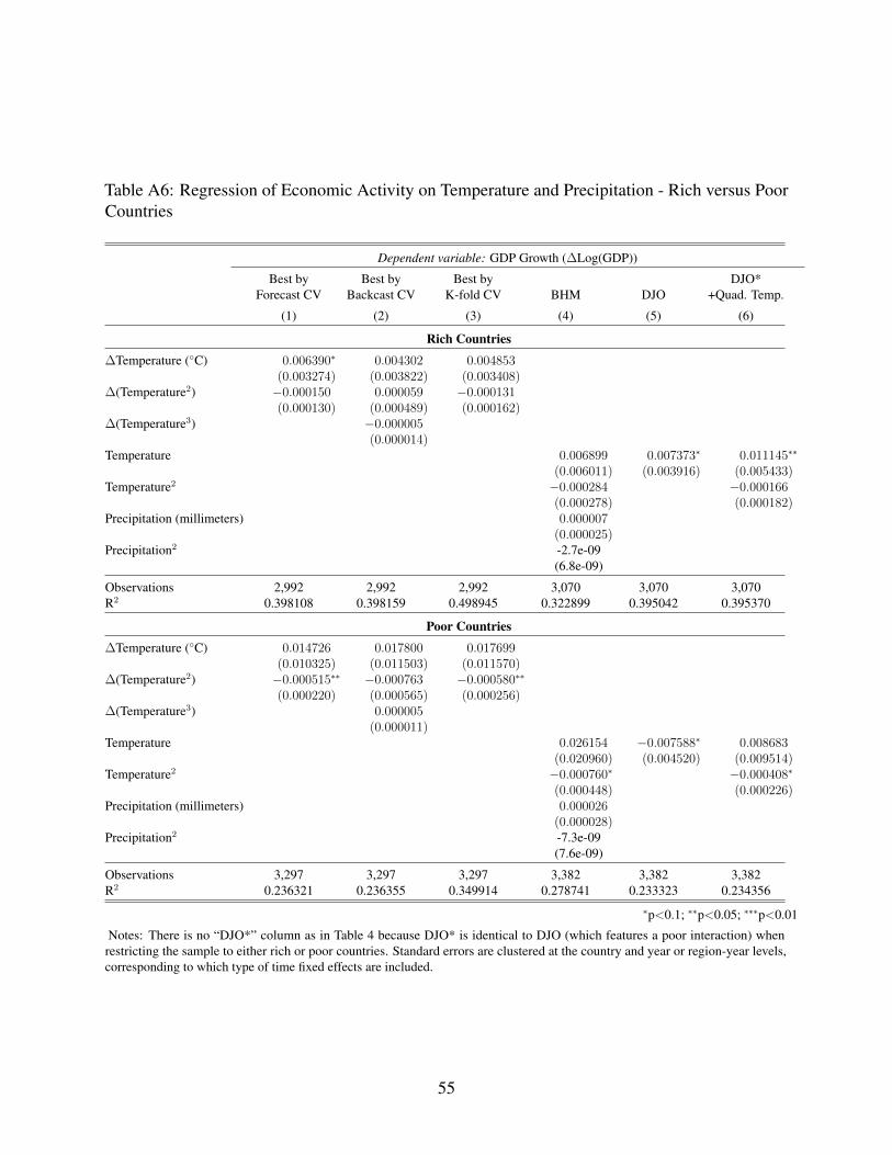
Table A6: Regression of Economic Activity on Temperature and Precipitation - Rich versus PoorCountries


Best by Best by Best by DJO*Forecast CV Backcast CV K-fold CV BHM DJO +Quad. Temp.

(1) (2) (3) (4) (5) (6)

Rich Countries

∆Temperature (◦C) 0.006390∗ 0.004302 0.004853(0.003274) (0.003822) (0.003408)

∆(Temperature2) −0.000150 0.000059 −0.000131(0.000130) (0.000489) (0.000162)

∆(Temperature3) −0.000005(0.000014)

Temperature 0.006899 0.007373∗ 0.011145∗∗

(0.006011) (0.003916) (0.005433)Temperature2 −0.000284 −0.000166

(0.000278) (0.000182)Precipitation (millimeters) 0.000007

(0.000025)Precipitation2 -2.7e-09

(6.8e-09)

Observations 2,992 2,992 2,992 3,070 3,070 3,070R2 0.398108 0.398159 0.498945 0.322899 0.395042 0.395370

Poor Countries

∆Temperature (◦C) 0.014726 0.017800 0.017699(0.010325) (0.011503) (0.011570)

∆(Temperature2) −0.000515∗∗ −0.000763 −0.000580∗∗

(0.000220) (0.000565) (0.000256)∆(Temperature3) 0.000005

(0.000011)Temperature 0.026154 −0.007588∗ 0.008683

(0.020960) (0.004520) (0.009514)Temperature2 −0.000760∗ −0.000408∗



(7.6e-09)

Observations 3,297 3,297 3,297 3,382 3,382 3,382R2 0.236321 0.236355 0.349914 0.278741 0.233323 0.234356

∗p<0.1; ∗∗p<0.05; ∗∗∗p<0.01

Notes: There is no “DJO*” column as in Table 4 because DJO* is identical to DJO (which features a poor interaction) whenrestricting the sample to either rich or poor countries. Standard errors are clustered at the country and year or region-year levels,corresponding to which type of time fixed effects are included.

55

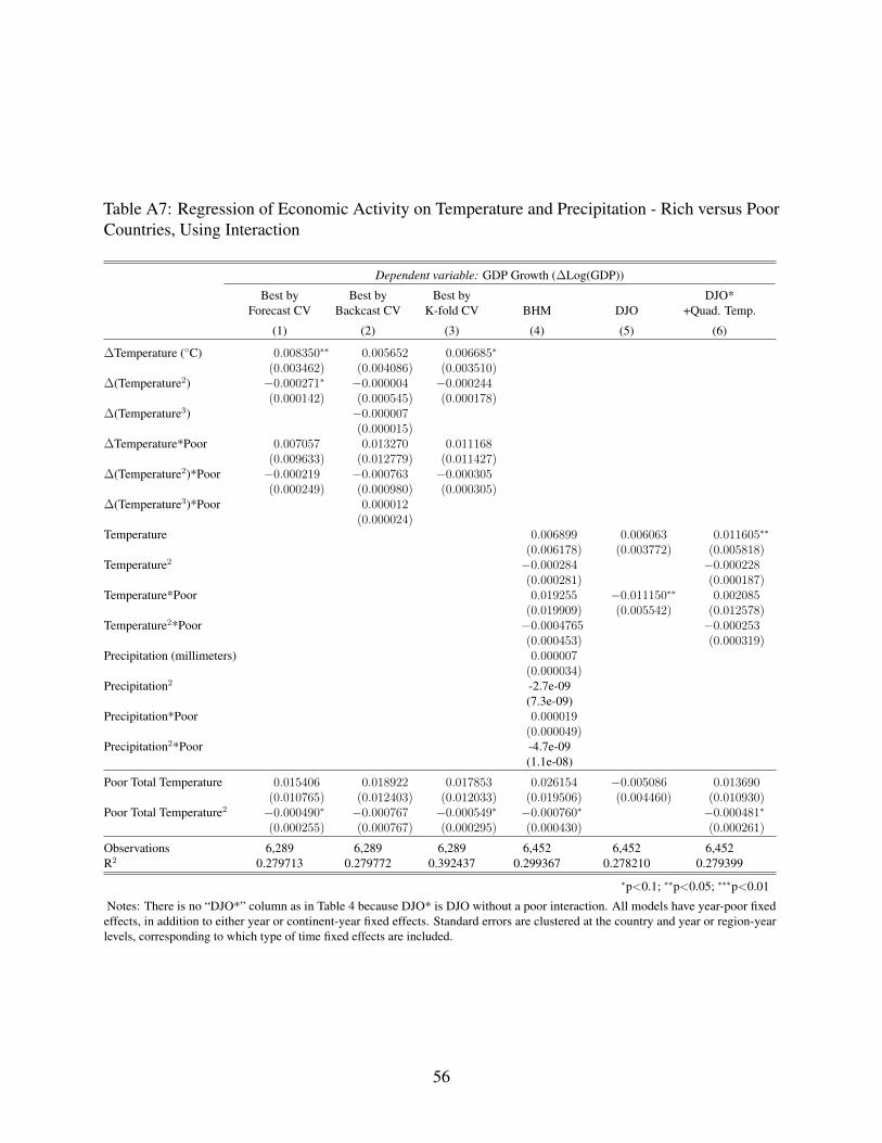
Table A7: Regression of Economic Activity on Temperature and Precipitation - Rich versus PoorCountries, Using Interaction


Best by Best by Best by DJO*Forecast CV Backcast CV K-fold CV BHM DJO +Quad. Temp.

(1) (2) (3) (4) (5) (6)

∆Temperature (◦C) 0.008350∗∗ 0.005652 0.006685∗

(0.003462) (0.004086) (0.003510)∆(Temperature2) −0.000271∗ −0.000004 −0.000244

(0.000142) (0.000545) (0.000178)∆(Temperature3) −0.000007

(0.000015)∆Temperature*Poor 0.007057 0.013270 0.011168

(0.009633) (0.012779) (0.011427)∆(Temperature2)*Poor −0.000219 −0.000763 −0.000305

(0.000249) (0.000980) (0.000305)∆(Temperature3)*Poor 0.000012

(0.000024)Temperature 0.006899 0.006063 0.011605∗∗

(0.006178) (0.003772) (0.005818)Temperature2 −0.000284 −0.000228

(0.000281) (0.000187)Temperature*Poor 0.019255 −0.011150∗∗ 0.002085

(0.019909) (0.005542) (0.012578)Temperature2*Poor −0.0004765 −0.000253



(7.3e-09)Precipitation*Poor 0.000019

(0.000049)Precipitation2*Poor -4.7e-09

(1.1e-08)

Poor Total Temperature 0.015406 0.018922 0.017853 0.026154 −0.005086 0.013690(0.010765) (0.012403) (0.012033) (0.019506) (0.004460) (0.010930)

Poor Total Temperature2 −0.000490∗ −0.000767 −0.000549∗ −0.000760∗ −0.000481∗

(0.000255) (0.000767) (0.000295) (0.000430) (0.000261)

Observations 6,289 6,289 6,289 6,452 6,452 6,452R2 0.279713 0.279772 0.392437 0.299367 0.278210 0.279399

∗p<0.1; ∗∗p<0.05; ∗∗∗p<0.01

Notes: There is no “DJO*” column as in Table 4 because DJO* is DJO without a poor interaction. All models have year-poor fixedeffects, in addition to either year or continent-year fixed effects. Standard errors are clustered at the country and year or region-yearlevels, corresponding to which type of time fixed effects are included.

56

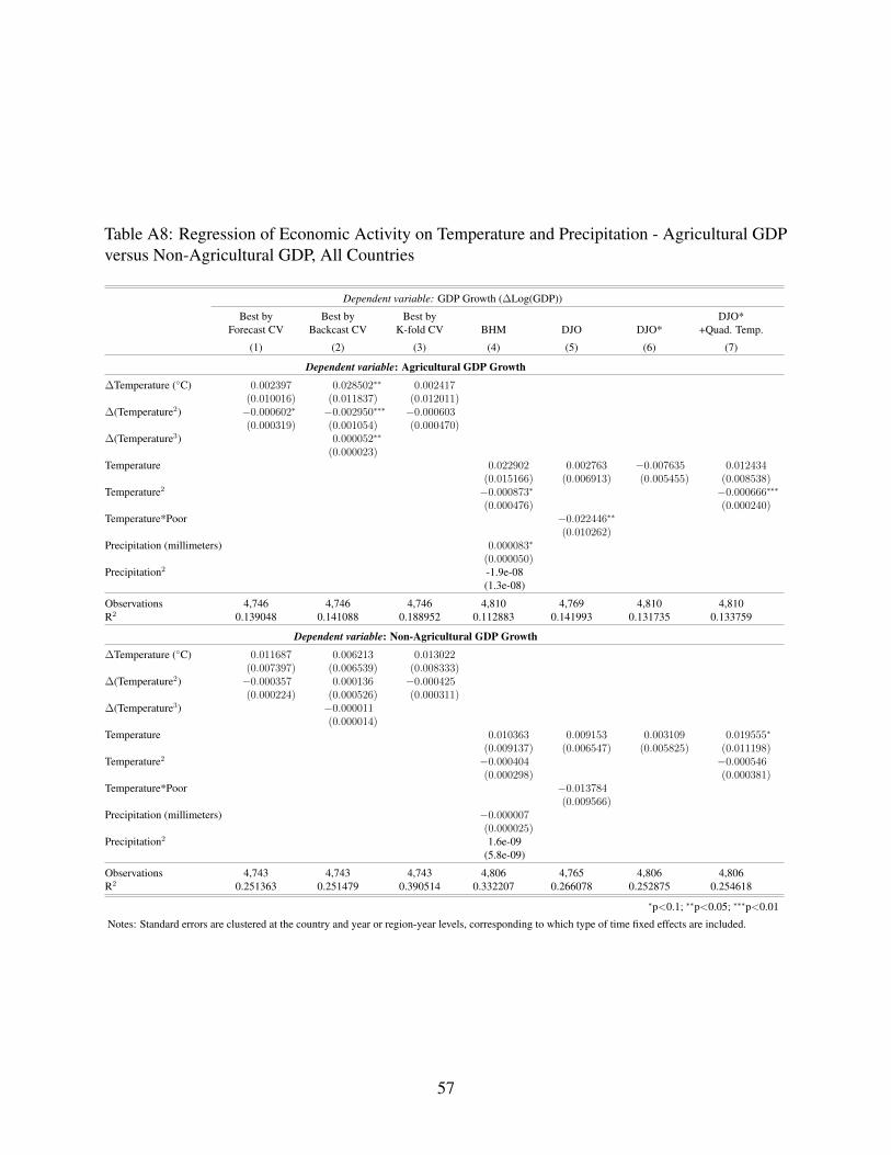
Table A8: Regression of Economic Activity on Temperature and Precipitation - Agricultural GDPversus Non-Agricultural GDP, All Countries


Best by Best by Best by DJO*Forecast CV Backcast CV K-fold CV BHM DJO DJO* +Quad. Temp.

(1) (2) (3) (4) (5) (6) (7)

Dependent variable: Agricultural GDP Growth

∆Temperature (◦C) 0.002397 0.028502∗∗ 0.002417(0.010016) (0.011837) (0.012011)

∆(Temperature2) −0.000602∗ −0.002950∗∗∗ −0.000603(0.000319) (0.001054) (0.000470)

∆(Temperature3) 0.000052∗∗

(0.000023)Temperature 0.022902 0.002763 −0.007635 0.012434

(0.015166) (0.006913) (0.005455) (0.008538)Temperature2 −0.000873∗ −0.000666∗∗∗

(0.000476) (0.000240)Temperature*Poor −0.022446∗∗

(0.010262)Precipitation (millimeters) 0.000083∗


(1.3e-08)

Observations 4,746 4,746 4,746 4,810 4,769 4,810 4,810R2 0.139048 0.141088 0.188952 0.112883 0.141993 0.131735 0.133759

Dependent variable: Non-Agricultural GDP Growth

∆Temperature (◦C) 0.011687 0.006213 0.013022(0.007397) (0.006539) (0.008333)

∆(Temperature2) −0.000357 0.000136 −0.000425(0.000224) (0.000526) (0.000311)

∆(Temperature3) −0.000011(0.000014)

Temperature 0.010363 0.009153 0.003109 0.019555∗

(0.009137) (0.006547) (0.005825) (0.011198)Temperature2 −0.000404 −0.000546

(0.000298) (0.000381)Temperature*Poor −0.013784

(0.009566)Precipitation (millimeters) −0.000007

(0.000025)Precipitation2 1.6e-09

(5.8e-09)

Observations 4,743 4,743 4,743 4,806 4,765 4,806 4,806R2 0.251363 0.251479 0.390514 0.332207 0.266078 0.252875 0.254618

∗p<0.1; ∗∗p<0.05; ∗∗∗p<0.01

Notes: Standard errors are clustered at the country and year or region-year levels, corresponding to which type of time fixed effects are included.

57

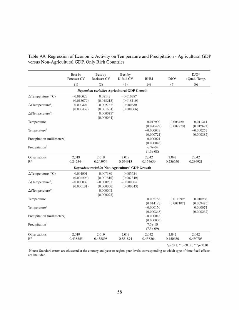
Table A9: Regression of Economic Activity on Temperature and Precipitation - Agricultural GDPversus Non-Agricultural GDP, Only Rich Countries

Best by Best by Best by DJO*Forecast CV Backcast CV K-fold CV BHM DJO* +Quad. Temp.

(1) (2) (3) (4) (5) (6)


∆Temperature (◦C) −0.010029 0.02142 −0.010387(0.013672) (0.018212) (0.018119)

∆(Temperature2) 0.000324 −0.002737∗ 0.000330(0.000459) (0.001504) (0.000666)

∆(Temperature3) 0.000075∗∗

(0.000034)Temperature 0.017990 0.005429 0.011314

(0.020429) (0.007273) (0.012621)Temperature2 −0.000649 −0.000253



(1.6e-08)

Observations 2,019 2,019 2,019 2,042 2,042 2,042R2 0.242544 0.245954 0.294913 0.154659 0.236650 0.236921


∆Temperature (◦C) 0.004901 0.007180 0.005524(0.005295) (0.007516) (0.007349)

∆(Temperature2) −0.000039 −0.000261 −0.000084(0.000181) (0.000866) (0.000343)

∆(Temperature3) 0.000005(0.000022)

Temperature 0.002783 0.011992∗ 0.010266(0.014123) (0.007107) (0.009475)

Temperature2 −0.000150 0.000074(0.000348) (0.000232)

Precipitation (millimeters) −0.000015(0.000036)

Precipitation2 7.5e-10(7.3e-09)

Observations 2,019 2,019 2,019 2,042 2,042 2,042R2 0.438855 0.438898 0.581874 0.458264 0.450650 0.450705

∗p<0.1; ∗∗p<0.05; ∗∗∗p<0.01

Notes: Standard errors are clustered at the country and year or region-year levels, corresponding to which type of time fixed effectsare included.

58

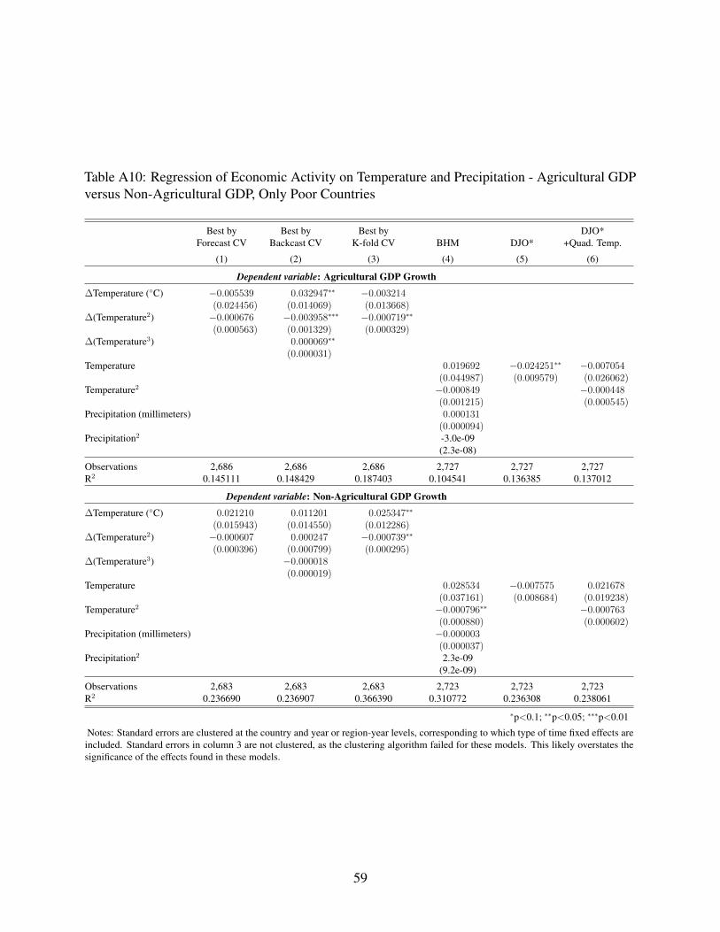
Table A10: Regression of Economic Activity on Temperature and Precipitation - Agricultural GDPversus Non-Agricultural GDP, Only Poor Countries

Best by Best by Best by DJO*Forecast CV Backcast CV K-fold CV BHM DJO* +Quad. Temp.

(1) (2) (3) (4) (5) (6)


∆Temperature (◦C) −0.005539 0.032947∗∗ −0.003214(0.024456) (0.014069) (0.013668)

∆(Temperature2) −0.000676 −0.003958∗∗∗ −0.000719∗∗

(0.000563) (0.001329) (0.000329)∆(Temperature3) 0.000069∗∗

(0.000031)Temperature 0.019692 −0.024251∗∗ −0.007054

(0.044987) (0.009579) (0.026062)Temperature2 −0.000849 −0.000448



(2.3e-08)

Observations 2,686 2,686 2,686 2,727 2,727 2,727R2 0.145111 0.148429 0.187403 0.104541 0.136385 0.137012


∆Temperature (◦C) 0.021210 0.011201 0.025347∗∗

(0.015943) (0.014550) (0.012286)∆(Temperature2) −0.000607 0.000247 −0.000739∗∗

(0.000396) (0.000799) (0.000295)∆(Temperature3) −0.000018

(0.000019)Temperature 0.028534 −0.007575 0.021678

(0.037161) (0.008684) (0.019238)Temperature2 −0.000796∗∗ −0.000763

(0.000880) (0.000602)Precipitation (millimeters) −0.000003

(0.000037)Precipitation2 2.3e-09

(9.2e-09)

Observations 2,683 2,683 2,683 2,723 2,723 2,723R2 0.236690 0.236907 0.366390 0.310772 0.236308 0.238061

∗p<0.1; ∗∗p<0.05; ∗∗∗p<0.01

Notes: Standard errors are clustered at the country and year or region-year levels, corresponding to which type of time fixed effects areincluded. Standard errors in column 3 are not clustered, as the clustering algorithm failed for these models. This likely overstates thesignificance of the effects found in these models.

59

Documents

The GDP-Temperature Relationship: Implications for Climate