Reinforcement Learning with Particle Swarm Optimization

DOI: 10.4018/IJSIR.2016070102

Copyright © 2016, IGI Global. Copying or distributing in print or electronic forms without written permission of IGI Global is prohibited.

International Journal of Swarm Intelligence ResearchVolume 7 • Issue 3 • July-September 2016

Reinforcement Learning with Particle Swarm Optimization Policy (PSO-P) in Continuous State and Action SpacesDaniel Hein, Technische, Universität München, Munich, Germany

Alexander Hentschel, Siemens AG, Munich, Germany

Thomas A. Runkler, Siemens AG, Munich, Germany

Steffen Udluft, Siemens AG, Munich, Germany

ABSTRACT

This article introduces a model-based reinforcement learning (RL) approach for continuous state and action spaces. While most RL methods try to find closed-form policies, the approach taken here employs numerical on-line optimization of control action sequences. First, a general method for reformulating RL problems as optimization tasks is provided. Subsequently, Particle Swarm Optimization (PSO) is applied to search for optimal solutions. This Particle Swarm Optimization Policy (PSO-P) is effective for high dimensional state spaces and does not require a priori assumptions about adequate policy representations. Furthermore, by translating RL problems into optimization tasks, the rich collection of real-world inspired RL benchmarks is made available for benchmarking numerical optimization techniques. The effectiveness of PSO-P is demonstrated on the two standard benchmarks: mountain car and cart pole.

KeywORdSBenchmark, Cart Pole, Continuous Action Space, Continuous State Space, High-dimensional, Model-based, Mountain Car, Particle Swarm Optimization, Reinforcement Learning

INTROdUCTION

Reinforcement learning (RL) is an area of machine learning inspired by biological learning. Formally, a software agent interacts with a system in discrete time steps. At each time step, the agent observes the system’s state s and applies an action a . Depending on s and a , the system transitions into a new state and the agent receives a real-valued reward r∈ . The agent’s goal is to maximize its expected cumulative reward, called return . The solution to an RL problem is a policy, i.e. a map that generates an action for any given state.

This article focuses on the most general RL setting with continuous state and action spaces. In this domain, the policy performance often strongly depends on the algorithms for policy generation and the chosen policy representation (Sutton & Barto, 1998). In the authors’ experience, tuning the policy-learning process is generally challenging for industrial RL problems. Specifically, it is hard to assess whether a trained policy has unsatisfactory performance due to inadequate training data, unsuitable policy representation, or an unfitting training algorithm. Determining the best problem-specific RL approach often requires time-intensive trials with different policy configurations and

23


24

training algorithms. In contrast, it is often significantly easier to train a well-performing system model from observational data, compared to directly learning a policy and assessing its performance.

To bypass the challenges of learning a closed-form RL policy, the authors adapted an approach from model-predictive control (Rawlings & Mayne, 2009; Camacho & Alba, 2007), which employs only a system model. The general idea behind model-predictive control is deceptively simple: given a reliable system model, one can predict the future evolution of the system and determine a control strategy that results in the desired system behavior. However, complex industry systems and plants commonly exhibit nonlinear system dynamics (Schaefer, Schneegass, Sterzing, & Udluft, 2007; Piche, et al., 2000). In such cases, closed-form solutions to the optimal control problem often do not exist or are computationally intractable to find (Findeisen & Allgoewer, 2002; Magni & Scattolini, 2004). Therefore, model-predictive control tasks for nonlinear systems are typically solved by numerical on-line optimization of sequences of control actions (Gruene & Pannek, 2011). Unfortunately, the resulting optimization problems are generally non-convex (Johansen, 2011) and no universal method for tackling nonlinear model-predictive control tasks has been found (Findeisen, Allgoewer, & Biegler, 2007; Rawlings, Tutorial overview of model predictive control, 2000). Moreover, one might argue based on theoretical considerations that such a universal optimization algorithm does not exist (Wolpert & Macready, 1997).

The main purpose of the present contribution is to provide a heuristic for solving RL problems which employs numerical on-line optimization of control action sequences. As an initial step, a neural system model is trained from observational data with standard methods. However, the presented method also works with any other model type, e.g., Gaussian process or physical models. The resulting problem of finding optimal control action sequences based on model predictions is solved with Particle Swarm Optimization (PSO), because PSO is an established algorithm for non-convex optimization. Specifically, the presented heuristic iterates over the following steps. (1) PSO is employed to search for an action sequence that maximizes the expected return when applied to the current system state by simulating its effects using the system model. (2) The first action of the sequence with the highest expected return is applied to the real-world system. (3) The system transitions to the subsequent state and the optimization process is repeated based on the new state (go to step 1).

As this approach can generate control actions for any system state, it formally constitutes an RL policy. This Particle Swarm Optimization Policy (PSO-P) deviates fundamentally from common RL approaches. Most methods for solving RL problems try to learn a closed-form policy (Sutton & Barto, 1998).The most significant advantages of PSO-P are the following. (1) Closed-form policy learners generally select a policy from a user-parameterized (potentially infinite) set of candidate policies. For example, when learning an RL policy based on tile coding (Sutton, 1996), the user must specify partitions of the state space. The partition’s characteristics directly influence how well the resulting policy can discriminate the effect of different actions. For complex RL problems, policy performances usually vary drastically depending on the chosen partitions. In contrast, PSO-P does not require a priori assumptions about problem-specific policy representations because it directly optimizes action sequences. (2) Closed-form RL policies operate on the state space and are generally affected by the curse of dimensionality (Bellmann, 1962). Simply put, the number of data points required for a representative coverage of the state space grows exponentially with the state space’s dimensionality. Common RL methods, such as tile coding, quickly become computationally intractable with increasing dimensionality. Moreover, for industrial RL problems it is often very expensive to obtain adequate training data prohibiting data-intensive RL methods. In comparison, PSO-P is not affected by the state space dimensionality because it operates in the space of action sequences.

From a strictly mathematical standpoint, PSO-P follows a known strategy from nonlinear model-predictive control: employ on-line numerical optimization to search for the best action sequences. While model-predictive control and RL target almost the same class of control-optimization problems with different methods, the mathematical formalisms in both communities are drastically different. Particularly, the authors find that the presented approach is rarely considered in the RL community.


25

The main contribution of this work is to provide a hands-on guide for employing on-line optimization of action sequences in the mathematical RL framework and demonstrate its effectiveness for solving RL problems. On the one hand, PSO-P generally requires significantly more computation time to determine an action for a given system state compared to closed-form RL policies. On the other hand, the authors found PSO-P particularly useful for determining the optimization potentials of various industrial control-optimization problems and for benchmarking other RL methods.

PSO and evolutionary algorithms are established heuristics for solving non-convex optimization problems. Both have been applied in the context of RL, however, almost exclusively to optimize policies directly. Moriarty, Schultz, and Grefenstette (1999) give a comprehensive overview of the various approaches using evolutionary algorithms to tackle RL problems. Methods which apply PSO to generate policies for specific system control problems were studied in (Feng, 2005), (Solihin & Akmeliawati, 2010), and (Montazeri-Gh, Jafari, & Ilkhani, 2012). However, these approaches do not generalize to RL, as expert-designed objective functions were used that already contained detailed knowledge about the optimal solution to the respective control problem. In contrast, in the present article, the general RL is reformulated as an optimization problem. This representation allows searching for optimal action sequences based on a system model, even if no expert knowledge about the underlying problem dynamics is available.

In the next two sections, the methods employed in this work are introduced, starting by formulating RL as a non-convex optimization problem and subsequently describing PSO-P as solver for this problem. The results of conducted benchmark experiments are subject of the section ‘Experiments, Results and Analysis’. Discussion of these results and limitations of PSO-P follow in the final section ‘Conclusions’.

FORMULATION OF ReINFORCeMeNT LeARNING AS OPTIMIZATION PROBLeM

In this article, the problem of optimizing the behavior of a physical system that is observed in discrete, equally spaced time steps t ∈ � is considered. The current time is denoted as t = 0 , t =1 and t = −1 represent one step into the future and one step into the past, respectively. At each time step t , the system is described by its Markovian state st ∈ , from the state space , and the agent’s action at is represented by a vector of I different control parameters, i.e. at

I∈ ⊂ . Based on the system’s state and the applied action, the system transitions into the state st+1 and the agent receives the reward rt .

In the following, deterministic systems which are described by a state transition function m :S A S× → × with m s a s rt t t t( , ) ( , )= +1 are considered.

The goal is to find an action sequence x = …+ + −( , , , )a a at t t T1 1 that maximizes the expected return . The search space is bounded by xmin and xmax which are defined by:

xmin minj j Ia j I T= ∀ = … ⋅ −

( mod ), ,0 1 (1)

and

xmax maxj j Ia j I T= ∀ = … ⋅ −

( mod ), ,0 1 (2)

where amin ( amax ) are the lower (upper) bounds of the control parameters.To incorporate the increasing uncertainty when planning actions further and further into the

future, the simulated reward rt k+

for k time steps into the future is weighted by γ k , where γ ∈[ , ]0 1 is referred to as the discount factor.


26

A common strategy is to simulate the system evolution only for a finite number of T ≥1 steps. The return is (Sutton & Barto, 1998)

( , ) , ( , ) ( , ).s r s r m s atk

k

T

t k t k t k t k t kx = ==

−

+ + + + + +∑γ0

1

1with (3)

The authors chose γ such that at the end of the time horizon T , the last reward accounted for is weighted by the user-defined constant q∈[ , ]0 1 , which implies γ = −q T1 1/( ) .

Solving the RL problem corresponds to finding the optimal action sequence x by maximizing

x xx

∈∈

argmax ( ),T

tfs (4)

with respect to the fitness function fsI T

t:

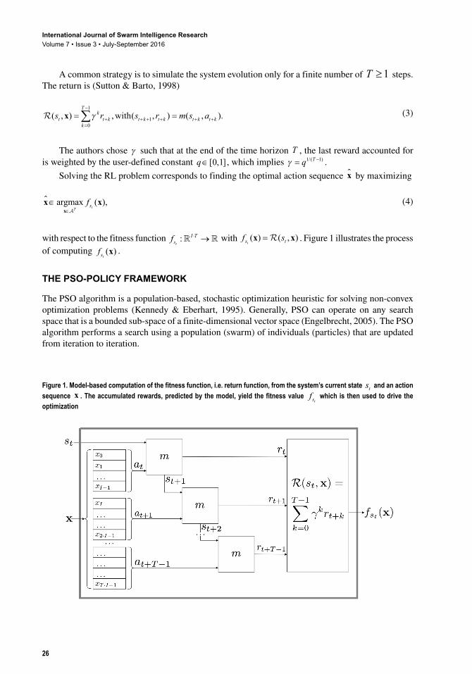
⋅ → with f ss tt( ) ( , )x x= . Figure 1 illustrates the process

of computing fst ( )x .

THe PSO-POLICy FRAMewORK

The PSO algorithm is a population-based, stochastic optimization heuristic for solving non-convex optimization problems (Kennedy & Eberhart, 1995). Generally, PSO can operate on any search space that is a bounded sub-space of a finite-dimensional vector space (Engelbrecht, 2005). The PSO algorithm performs a search using a population (swarm) of individuals (particles) that are updated from iteration to iteration.

Figure 1. Model-based computation of the fitness function, i.e. return function, from the system’s current state st and an action sequence x . The accumulated rewards, predicted by the model, yield the fitness value fst which is then used to drive the optimization


27

In this article PSO is used to solve, i.e. the particles move through the search space of action sequences T . Consequently, a particle’s position represents a candidate action sequence x = …+ + −( , , , )a a at t t T1 1 , which is initially chosen at random.

At each iteration, particle i remembers its local best position, y i , that it has visited so far (including its current position). Furthermore, particle i also knows the neighborhood best position

y zz y

ip j

p fj i

( ) argmax ( ),{ ( ) }

+ ∈∈ ∈

1|

(5)

found so far by any one particle in its neighborhood i (including itself). The neighborhood relations between particles are determined by the swarm’s population topology and are generally fixed, irrespective of the particles’ positions.

In the experiments presented in Section Experiments, Results and Analysis the authors use the ring topology (Eberhart, Simpson, & Dobbins, 1996).

From iteration p to p +1 the particle position update rule is

x x vi i ip p p( ) ( ) ( ).+ = + +1 1 (6)

The components of the velocity vector v are calculated by

v p wv p c r p y p x pij ij j ij ij( ) ( ) ( )[ ( ) ( )]+ = + −1 1 1

cognitive componentt social component� ��

��

+ −c r p y p x pj ij ij2 2 ( )[ ( ) ( )]��

, (7)

where w is the inertia weight factor, v pij ( ) and x pij ( ) are the velocity and the position of particle i in dimension j , c1 and c2 are positive acceleration constants used to scale the contribution of the cognitive and the social components y pij ( ) and y pij

( ) respectively. The factors r pj1 ( ) , r p Uj2 0 1( ) ~ ( , ) are random values sampled from a uniform distribution to introduce a stochastic element to the algorithm. Shi and Eberhart (2000) proposed to set the values to w = 0 7298. and c c1 2 1 49618 = = . .

Even though a sequence of T actions is optimized, only the first action is applied to the real world system and an optimization of a new action sequence is performed for the subsequent system state st+1 . Therefore, model inaccuracies have a significantly reduced impact compared to applying the entire action sequence at once.

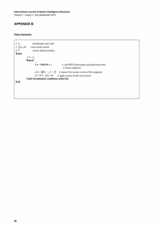
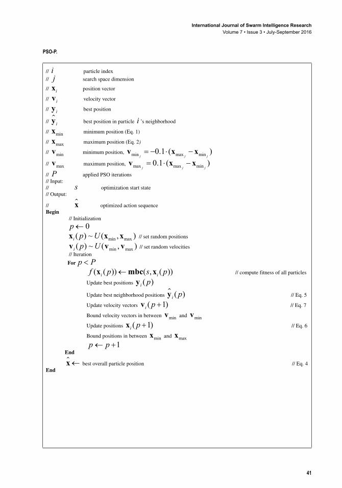
Implementation details can be found in Appendix B.

eXPeRIMeNTS, ReSULTS, ANd ANALySIS

The authors applied the PSO-P framework to two different RL problems. These two problems are the mountain car (Sutton & Barto, 1998) and the cart pole balancing benchmark (Fantoni & Lozano, 2002), which are used to illustrate the framework’s capability of solving RL problems in general.

For each benchmark, a neural network has been trained as the system model m using standard techniques (Montavon, Orr, & Müller, 2012). Neural networks are well suited for data-driven black-box models as they are universal approximators (Hornik, Stinchcombe, & White, 1989) and the authors found that the resulting models generalize well to new data in many real-world applications.

The authors have chosen this approach, instead of working directly with benchmark simulations because in many real-world scenarios physical simulations are either unavailable or strongly idealized.


28

However, PSO-P works with other model types as well, such as physical or Gaussian process models (Rasmussen & Williams, 2006).

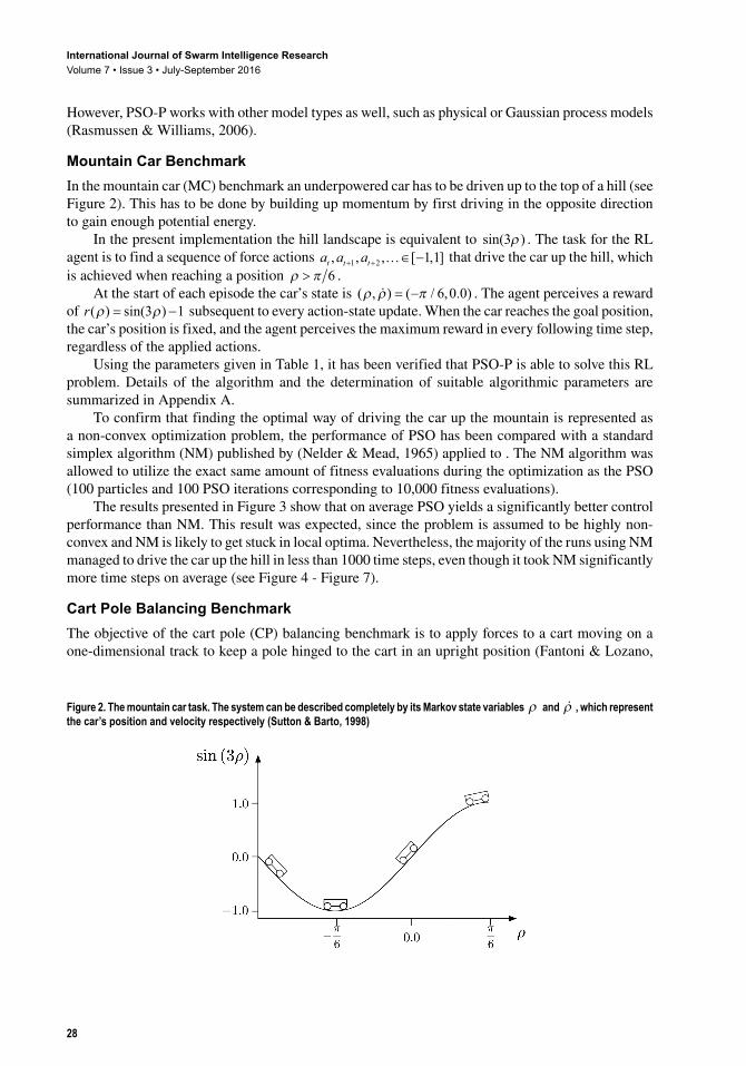
Mountain Car BenchmarkIn the mountain car (MC) benchmark an underpowered car has to be driven up to the top of a hill (see Figure 2). This has to be done by building up momentum by first driving in the opposite direction to gain enough potential energy.

In the present implementation the hill landscape is equivalent to sin( )3ρ . The task for the RL agent is to find a sequence of force actions a a at t t, , , [ , ]+ + …∈ −1 2 1 1 that drive the car up the hill, which is achieved when reaching a position ρ π> 6 .

At the start of each episode the car’s state is ( , ) ( / , . )ρ ρ π = − 6 0 0 . The agent perceives a reward of r( ) sin( )ρ ρ= −3 1 subsequent to every action-state update. When the car reaches the goal position, the car’s position is fixed, and the agent perceives the maximum reward in every following time step, regardless of the applied actions.

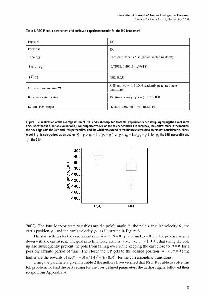
Using the parameters given in Table 1, it has been verified that PSO-P is able to solve this RL problem. Details of the algorithm and the determination of suitable algorithmic parameters are summarized in Appendix A.

To confirm that finding the optimal way of driving the car up the mountain is represented as a non-convex optimization problem, the performance of PSO has been compared with a standard simplex algorithm (NM) published by (Nelder & Mead, 1965) applied to . The NM algorithm was allowed to utilize the exact same amount of fitness evaluations during the optimization as the PSO (100 particles and 100 PSO iterations corresponding to 10,000 fitness evaluations).

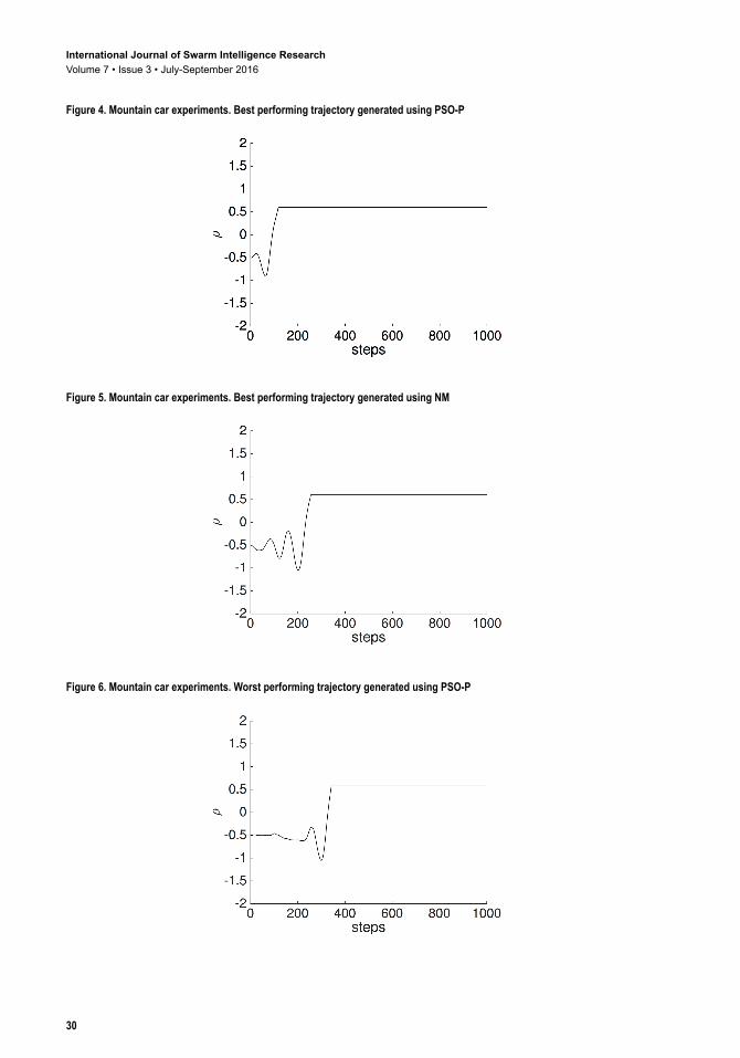
The results presented in Figure 3 show that on average PSO yields a significantly better control performance than NM. This result was expected, since the problem is assumed to be highly non-convex and NM is likely to get stuck in local optima. Nevertheless, the majority of the runs using NM managed to drive the car up the hill in less than 1000 time steps, even though it took NM significantly more time steps on average (see Figure 4 - Figure 7).

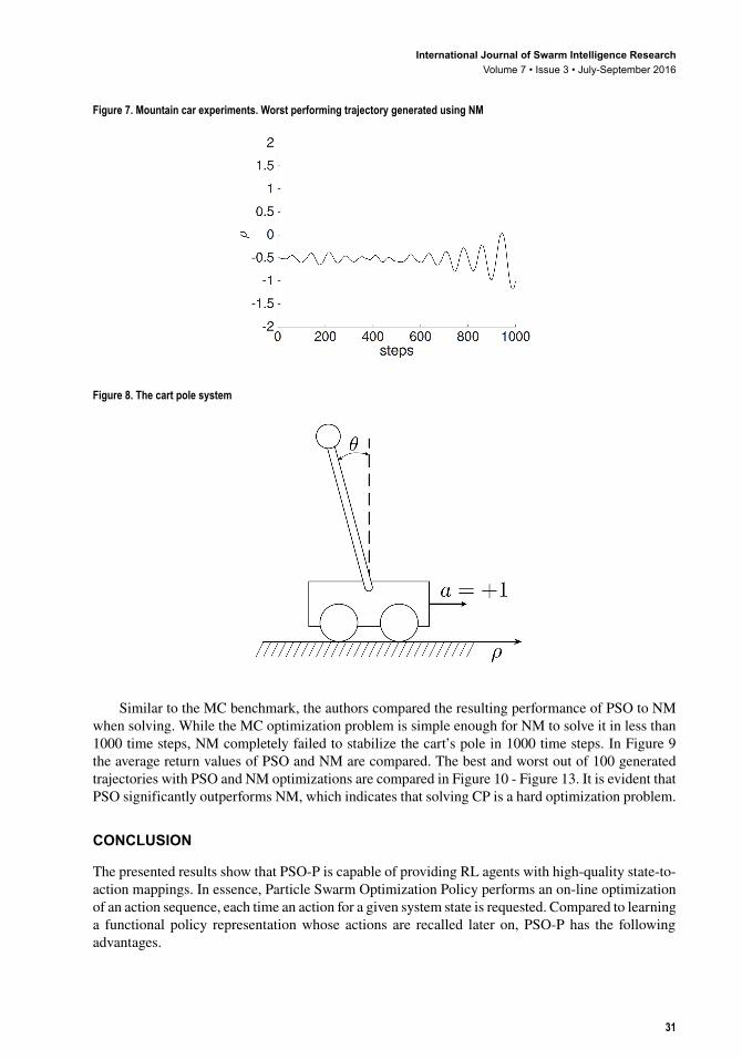
Cart Pole Balancing BenchmarkThe objective of the cart pole (CP) balancing benchmark is to apply forces to a cart moving on a one-dimensional track to keep a pole hinged to the cart in an upright position (Fantoni & Lozano,

Figure 2. The mountain car task. The system can be described completely by its Markov state variables ρ and ρ , which represent the car’s position and velocity respectively (Sutton & Barto, 1998)


29

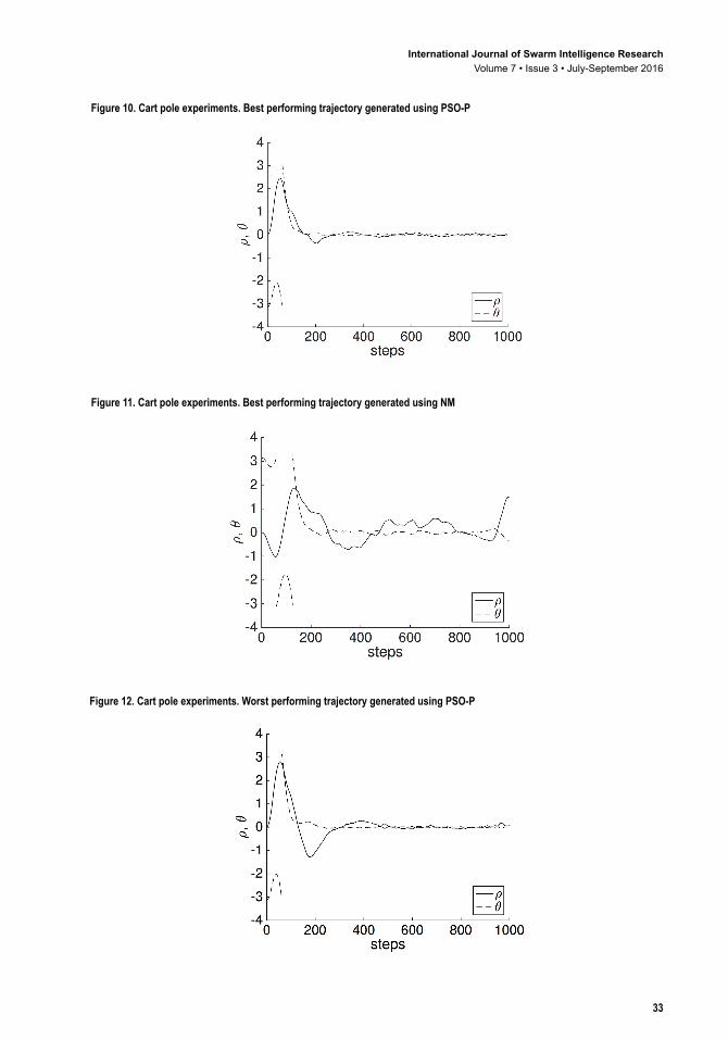
2002). The four Markov state variables are the pole’s angle θ , the pole’s angular velocity θ , the cart’s position ρ , and the cart’s velocity ρ , as illustrated in Figure 8.

The start settings for the experiments are: θ π= , θ = 0 , ρ = 0 , and ρ = 0 , i.e. the pole is hanging down with the cart at rest. The goal is to find force actions a a at t t, , , [ , ]+ + …∈ −1 2 1 1 , that swing the pole up and subsequently prevent the pole from falling over while keeping the cart close to ρ = 0 for a possibly infinite period of time. The closer the CP gets to the desired position (θ = 0 , ρ = 0 ) the higher are the rewards r( , ) ( / . ) ( / . )ρ θ ρ θ= − +1 4 0 32 2 for the corresponding transitions.

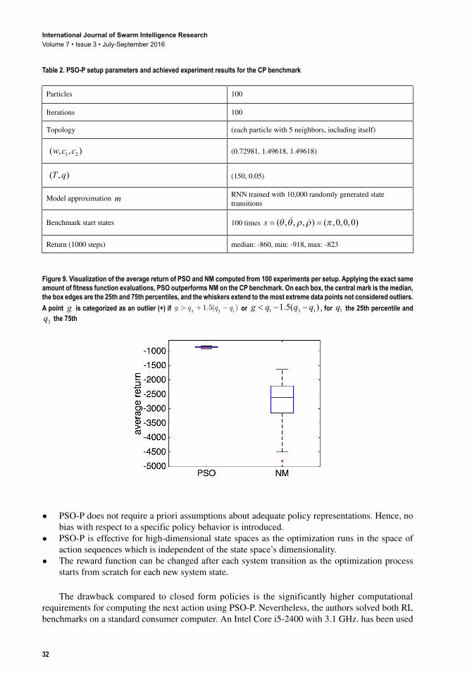
Using the parameters given in Table 2 the authors have verified that PSO-P is able to solve this RL problem. To find the best setting for the user-defined parameters the authors again followed their recipe from Appendix A.

Table 1. PSO-P setup parameters and achieved experiment results for the MC benchmark

Particles 100

Iterations 100

Topology (each particle with 5 neighbors, including itself)

( , , )w c c1 2 (0.72981, 1.49618, 1.49618)

( , )T q (100, 0.05)

Model approximation m RNN trained with 10,000 randomly generated state transitions

Benchmark start states 100 times s = = −( , ) ( / , . )ρ ρ π 6 0 0

Return (1000 steps) median: -350, min: -644, max: -197

Figure 3. Visualization of the average return of PSO and NM computed from 100 experiments per setup. Applying the exact same amount of fitness function evaluations, PSO outperforms NM on the MC benchmark. On each box, the central mark is the median, the box edges are the 25th and 75th percentiles, and the whiskers extend to the most extreme data points not considered outliers. A point g is categorized as an outlier (+) if g q q q> + −3 3 11 5. ( ) or g q q q< − −1 3 11 5. ( ) , for q1 the 25th percentile and q3 the 75th


30

Figure 4. Mountain car experiments. Best performing trajectory generated using PSO-P

Figure 5. Mountain car experiments. Best performing trajectory generated using NM

Figure 6. Mountain car experiments. Worst performing trajectory generated using PSO-P


31

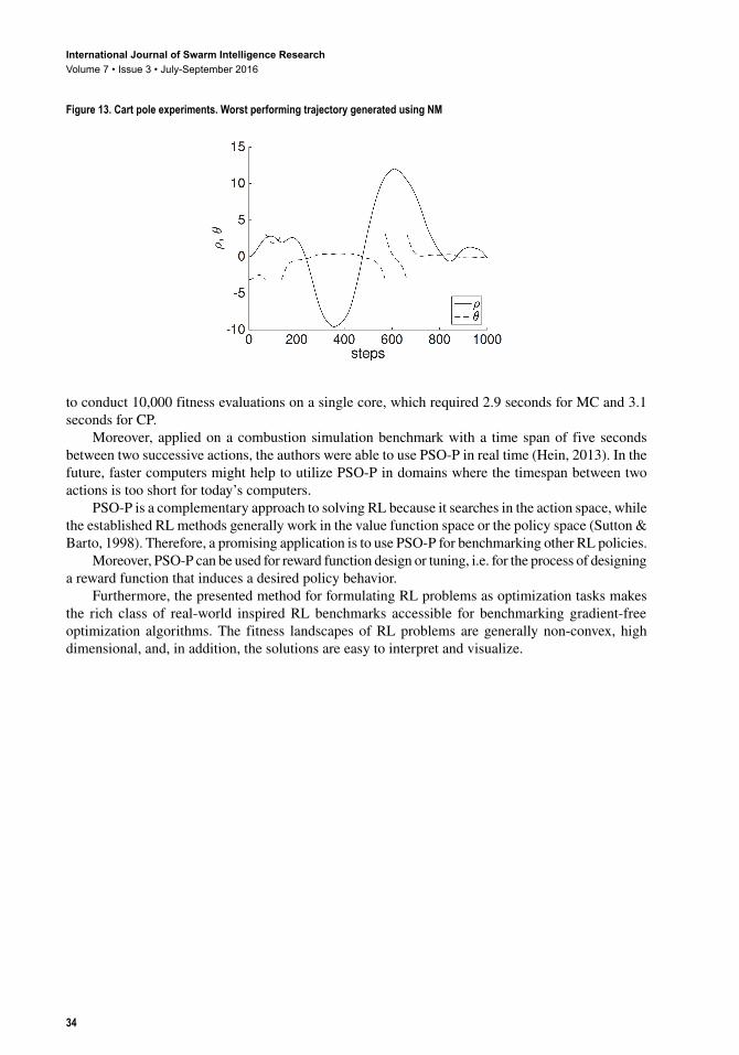
Similar to the MC benchmark, the authors compared the resulting performance of PSO to NM when solving. While the MC optimization problem is simple enough for NM to solve it in less than 1000 time steps, NM completely failed to stabilize the cart’s pole in 1000 time steps. In Figure 9 the average return values of PSO and NM are compared. The best and worst out of 100 generated trajectories with PSO and NM optimizations are compared in Figure 10 - Figure 13. It is evident that PSO significantly outperforms NM, which indicates that solving CP is a hard optimization problem.

CONCLUSION

The presented results show that PSO-P is capable of providing RL agents with high-quality state-to-action mappings. In essence, Particle Swarm Optimization Policy performs an on-line optimization of an action sequence, each time an action for a given system state is requested. Compared to learning a functional policy representation whose actions are recalled later on, PSO-P has the following advantages.

Figure 7. Mountain car experiments. Worst performing trajectory generated using NM

Figure 8. The cart pole system


32

• PSO-P does not require a priori assumptions about adequate policy representations. Hence, no bias with respect to a specific policy behavior is introduced.

• PSO-P is effective for high-dimensional state spaces as the optimization runs in the space of action sequences which is independent of the state space’s dimensionality.

• The reward function can be changed after each system transition as the optimization process starts from scratch for each new system state.

The drawback compared to closed form policies is the significantly higher computational requirements for computing the next action using PSO-P. Nevertheless, the authors solved both RL benchmarks on a standard consumer computer. An Intel Core i5-2400 with 3.1 GHz. has been used

Table 2. PSO-P setup parameters and achieved experiment results for the CP benchmark

Particles 100

Iterations 100

Topology (each particle with 5 neighbors, including itself)

( , , )w c c1 2 (0.72981, 1.49618, 1.49618)

( , )T q (150, 0.05)

Model approximation m RNN trained with 10,000 randomly generated state transitions

Benchmark start states 100 times s = =( , , , ) ( , , , )θ θ ρ ρ π

0 0 0

Return (1000 steps) median: -860, min: -918, max: -823

Figure 9. Visualization of the average return of PSO and NM computed from 100 experiments per setup. Applying the exact same amount of fitness function evaluations, PSO outperforms NM on the CP benchmark. On each box, the central mark is the median, the box edges are the 25th and 75th percentiles, and the whiskers extend to the most extreme data points not considered outliers. A point g is categorized as an outlier (+) if g q q q> + −

3 3 11 5. ( ) or g q q q< − −1 3 11 5. ( ) , for q1 the 25th percentile and

q3 the 75th


33

Figure 10. Cart pole experiments. Best performing trajectory generated using PSO-P

Figure 11. Cart pole experiments. Best performing trajectory generated using NM

Figure 12. Cart pole experiments. Worst performing trajectory generated using PSO-P


34

to conduct 10,000 fitness evaluations on a single core, which required 2.9 seconds for MC and 3.1 seconds for CP.

Moreover, applied on a combustion simulation benchmark with a time span of five seconds between two successive actions, the authors were able to use PSO-P in real time (Hein, 2013). In the future, faster computers might help to utilize PSO-P in domains where the timespan between two actions is too short for today’s computers.

PSO-P is a complementary approach to solving RL because it searches in the action space, while the established RL methods generally work in the value function space or the policy space (Sutton & Barto, 1998). Therefore, a promising application is to use PSO-P for benchmarking other RL policies.

Moreover, PSO-P can be used for reward function design or tuning, i.e. for the process of designing a reward function that induces a desired policy behavior.

Furthermore, the presented method for formulating RL problems as optimization tasks makes the rich class of real-world inspired RL benchmarks accessible for benchmarking gradient-free optimization algorithms. The fitness landscapes of RL problems are generally non-convex, high dimensional, and, in addition, the solutions are easy to interpret and visualize.

Figure 13. Cart pole experiments. Worst performing trajectory generated using NM


35

ReFeReNCeS

Bellmann, R. (1962). Adaptive Control Processes: A Guided Tour. Princeton University Press.

Camacho, F., & Alba, C. (2007). Model Predictive Control. London: Springer-Verlag; doi:10.1007/978-0-85729-398-5

Eberhart, R., & Shi, Y. (2000). Comparing Inertia Weigths and Constriction Factors in Particle Swarm Optimization.Proceedings of the IEEE Congress on Evolutionary Computation (Vol. 1, pp. 84–88).

Eberhart, R., Simpson, P., & Dobbins, R. (1996). Computational Intelligence PC Tools. San Diego, CA, USA: Academic Press Professional, Inc.

Engelbrecht, A. (2005). Fundamentals of Computational Swarm Intelligence. Wiley.

Fantoni, I., & Lozano, R. (2002). Non-linear Control for Underactuated Mechanical Systems. London: Springer; doi:10.1007/978-1-4471-0177-2

Feng, H.-M. (2005). Particle swarm optimization learning fuzzy systems design.Third International Conference on Information Technology and Applications (Vol. 1, pp. 363-366). doi:10.1109/ICITA.2005.206

Findeisen, R., & Allgoewer, F. (2002). An Introduction to Nonlinear Model Predictive Control.Proceedings of the 21st Benelux Meeting on Systems and Control (pp. 1-23).

Findeisen, R., Allgoewer, F., & Biegler, L. (2007). Assessment and Future Directions of Nonlinear Model Predictive Control. Berlin, Heidelberg: Springer-Verlag; doi:10.1007/978-3-540-72699-9

Gruene, L., & Pannek, J. (2011). Nonlinear Model Predictive Control. London: Springer-Verlag; doi:10.1007/978-0-85729-501-9

Hein, D. (2013). Particle Swarm Optimization for Finding an Optimal Action Sequence for a Gas Turbine Controller. Technical report. Technische Universität München.

Hornik, K., Stinchcombe, M., & White, H. (1989). Multilayer Feedforward Networks are Universal Approximators. Neural Networks, 2(5), 359–366. doi:10.1016/0893-6080(89)90020-8

Johansen, T. (2011). Introduction to Nonlinear Model Predictive Control and Moving Horizon Estimation. In M. Huba, S. Skogestad, M. Fikar, M. Hovd, T. Johansen, & B. Rohal-Ilkiv (Eds.), Selected Topics on Constrained and Nonlinear Control. Bratislava, Trondheim: STU Bratislava/NTNU Trondheim.

Kennedy, J., & Eberhart, R. (1995). Particle Swarm Optimization.Proceedings of IEEE International Conference on Neural Networks (Vol. 4, pp. 1942–1948). doi:10.1109/ICNN.1995.488968

Magni, L., & Scattolini, R. (2004). Stabilizing model predictive control of nonlinear continuous time systems. Annual Reviews in Control, 28(1), 1–11. doi:10.1016/j.arcontrol.2004.01.001

Montavon, G., Orr, G., & Müller, K. (2012). Neural Networks: Tricks of the Trade. Berlin, Heidelberg: Springer; doi:10.1007/978-3-642-35289-8

Montazeri-Gh, M., Jafari, S., & Ilkhani, M. (2012). Application of particle swarm optimization in gas turbine engine fuel controller gain tuning. Engineering Optimization, 44(2), 225–240. doi:10.1080/0305215X.2011.576760

Moriarty, D., Schultz, A., & Grefenstette, J. (1999). Evolutionary Algorithms for Reinforcement Learning. Journal of Artificial Intelligence Research, 11, 241–276.

Nelder, J., & Mead, R. (1965). A simplex method for function minimization. The Computer Journal, 7(4), 308–313. doi:10.1093/comjnl/7.4.308

Piche, S., Keeler, J., Martin, G., Boe, G., Johnson, D., & Gerules, M. (2000). Neural network based Model Predictive Control. Advances in Neural Information Processing Systems, 2000, 1029–1035.

Rasmussen, C., & Williams, C. (2006). Gaussian Processes for Machine Learning (Vol. Adaptive Computation and Machine Learning). MIT Press.

http://dx.doi.org/10.1007/978-0-85729-398-5

http://dx.doi.org/10.1007/978-0-85729-398-5

http://dx.doi.org/10.1007/978-1-4471-0177-2

http://dx.doi.org/10.1109/ICITA.2005.206

http://dx.doi.org/10.1007/978-3-540-72699-9

http://dx.doi.org/10.1007/978-0-85729-501-9

http://dx.doi.org/10.1007/978-0-85729-501-9

http://dx.doi.org/10.1016/0893-6080(89)90020-8

http://dx.doi.org/10.1109/ICNN.1995.488968

http://dx.doi.org/10.1016/j.arcontrol.2004.01.001

http://dx.doi.org/10.1007/978-3-642-35289-8

http://dx.doi.org/10.1080/0305215X.2011.576760

http://dx.doi.org/10.1080/0305215X.2011.576760

http://dx.doi.org/10.1093/comjnl/7.4.308


36

Rawlings, J. (2000). Tutorial overview of model predictive control. IEEE Control Systems Magazine, 20(3), 38–52. doi:10.1109/37.845037

Rawlings, J., & Mayne, D. (2009). Model Predictive Control Theory and Design. Nob Hill Publishing.

Schaefer, A., Schneegass, D., Sterzing, V., & Udluft, S. (2007). A neural reinforcement learning approach to gas turbine control.Proceedings of the IEEE International Conference on Neural Networks - Conference Proceedings (pp. 1691-1696). doi:10.1109/IJCNN.2007.4371212

Solihin, M., & Akmeliawati, R. (2010). Particle Swam Optimization for Stabilizing Controller of a Self-erecting Linear Inverted Pendulum. International Journal of Electrical and Electronic Systems Research, 2, 13–23.

Sutton, R. (1996). Generalization in Reinforcement Learning: Successful Examples Using Sparse Coarse Coding. Advances in Neural Information Processing Systems, 8, 1038–1044.

Sutton, R., & Barto, A. (1998). Reinforcement Learning: An Introduction. Cambridge, MA: MIT Press.

Wolpert, D., & Macready, W. (1997). No free lunch theorems for optimization. IEEE Transactions on Evolutionary Computation, 1(1), 67–82. doi:10.1109/4235.585893

Daniel Hein received his BSc degree in Computer Sciences from the University of Applied Sciences Zwickau, Germany, in 2011 and the MSc degree in Informatics from the Technische Universität München, Germany, in 2014. He is currently pursuing a PhD in Informatics at Technische Universität München, Germany, and is conducting his research in partnership with Siemens Corporate Technology. His research interests include evolutionary algorithms, like particle swarm optimization or genetic programming, interpretable reinforcement learning, and industrial application of machine learning approaches.

Alexander Hentschel graduated with a diploma degree in Physics (2007) and a diploma in Computer Science (2010) from the Humboldt-Universität zu Berlin, Germany. He did his doctorate research in the interdisciplinary field of quantum computing and quantum information science at the University of Calgary, Canada. There, he developed machine learning algorithms for quantum-enhanced measurement procedures. Since 2011 Alexander Hentschel has continued his research in the area of applied machine learning as a Research Scientist at Siemens Corporate Technology. His current focus is interpretable reinforcement learning and swarm algorithms.

Thomas Runkler received his MSc and PhD in electrical engineering from the Technical University of Darmstadt, Germany, in 1992 and 1995, respectively, and was a postdoctoral researcher at the University of West Florida from 1996-1997. He has been teaching computer science at the Technische Universität München, Germany, since 1999, and was appointed adjunct professor in 2011. Since 1997 he has been working for Siemens Corporate Technology in various expert and management functions, currently as a Principal Research Scientist. His main research interests include machine learning, data analysis, pattern recognition, and optimization.

Steffen Udluft received his diploma and PhD in physics from the Ludwig-Maximilians University München, in 1996 and 2000, respectively, and was a postdoctoral researcher at the Max-Planck-Institute for physics from 2000 to 2001. During this time he worked on the neuro-trigger of the H1 experiment for particle physics at DESY, Hamburg. Since 2001 he has been working for Siemens Corporate Technology, and continues to pursue the application of neural networks and other machine learning methods to real word problems. His main research focus is data-efficient reinforcement learning which includes transfer-learning, handling of uncertainty, and generalization capabilities.

http://dx.doi.org/10.1109/37.845037

http://dx.doi.org/10.1109/IJCNN.2007.4371212

http://dx.doi.org/10.1109/4235.585893


37

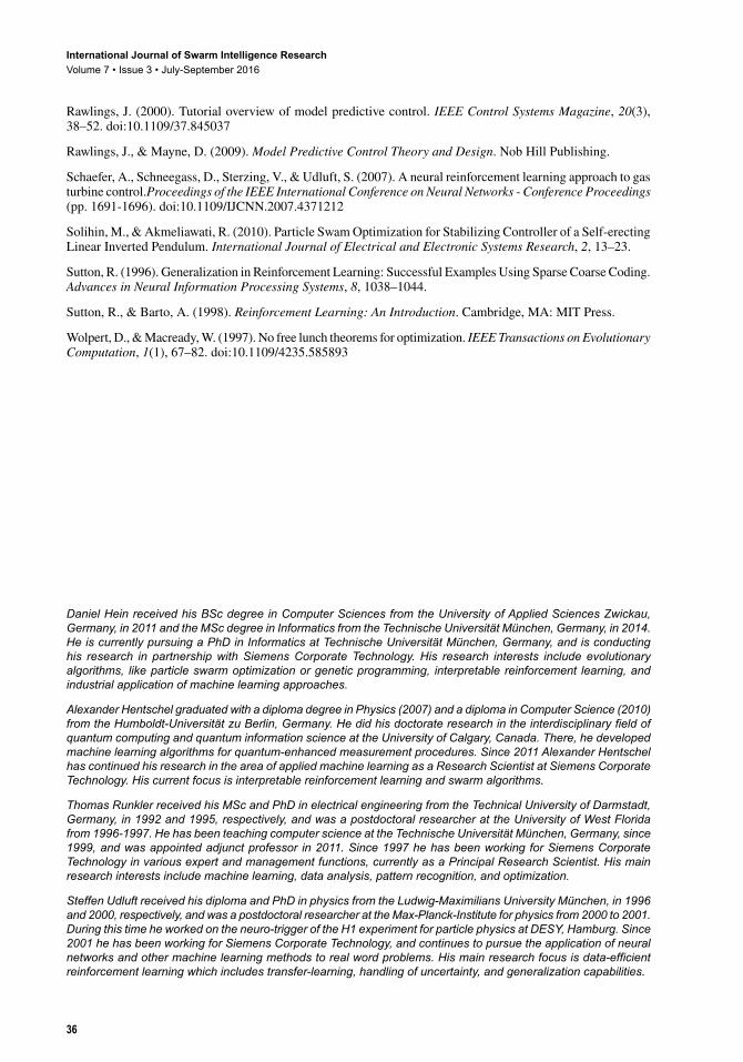
APPeNdIX A

Given a sufficiently trained model of the real system, the conducted experiments show that the following recipe successfully finds appropriate parameters for the PSO-P:

1. Start with the ring topology and an initial guess of the swarm size, depending on the intended computational effort.2. Evaluate the problem dependent time horizonT .3. Compare different topologies for both convergence properties; speed and quality of the found solutions.4. Determine the particle amount which leads to the best rewards, given a fixed level of computational effort.

In the following, an exemplary PSO-P parameter evaluation for the CP benchmark is described.The first step is to find a suitable time horizon for the RL problem. On the one hand, this horizon should be as short as possible to keep computational effort low. On the other hand, it has to be long enough to recognize all possible future effects of the current action. Figure 14 shows the results for time horizons of length 100, 150, 200 and 250 time steps. A time horizon length of 100 yields a relatively low average return compared to the horizon lengths 150, 200 and 250. The reason for this is that it is much harder for the PSO-P to determine whether an action sequence leads to constantly good results in the future if the time horizon is below 150 in the CP benchmark. The increase of the horizon above 150 did not yield better results, so the horizon of 150 seems to be a good compromise between stable results and fast computing.

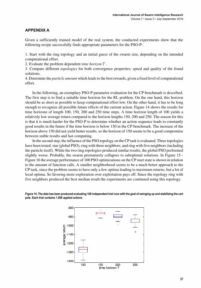
In the second step, the influence of the PSO topology on the CP task is evaluated. Three topologies have been tested: star (global PSO), ring with three neighbors, and ring with five neighbors (including the particle itself). While the two ring topologies produced similar results, the global PSO performed slightly worse. Probably, the swarm prematurely collapses to suboptimal solutions. In Figure 15 - Figure 16 the average performance of 100 PSO optimizations on the CP start state is shown in relation to the amount of function calls. A smaller neighborhood seems to be a much better approach to the CP task, since the problem seems to have only a few optima leading to maximum returns, but a lot of local optima. So favoring more exploration over exploitation pays off. Since the topology ring with five neighbors produced the best median result the experiments are continued using this topology.

Figure 14. The data has been produced evaluating 100 independent trial runs with the goal of swinging up and stabilizing the cart pole. Each trial contains 1,000 applied actions


38

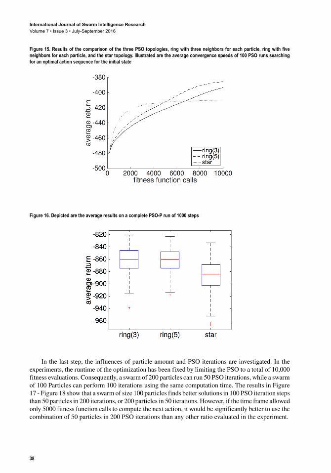
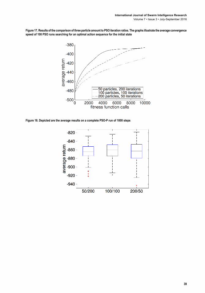
In the last step, the influences of particle amount and PSO iterations are investigated. In the experiments, the runtime of the optimization has been fixed by limiting the PSO to a total of 10,000 fitness evaluations. Consequently, a swarm of 200 particles can run 50 PSO iterations, while a swarm of 100 Particles can perform 100 iterations using the same computation time. The results in Figure 17 - Figure 18 show that a swarm of size 100 particles finds better solutions in 100 PSO iteration steps than 50 particles in 200 iterations, or 200 particles in 50 iterations. However, if the time frame allowed only 5000 fitness function calls to compute the next action, it would be significantly better to use the combination of 50 particles in 200 PSO iterations than any other ratio evaluated in the experiment.

Figure 15. Results of the comparison of the three PSO topologies, ring with three neighbors for each particle, ring with five neighbors for each particle, and the star topology. Illustrated are the average convergence speeds of 100 PSO runs searching for an optimal action sequence for the initial state

Figure 16. Depicted are the average results on a complete PSO-P run of 1000 steps


39

Figure 17. Results of the comparison of three particle amount to PSO iteration ratios. The graphs illustrate the average convergence speed of 100 PSO runs searching for an optimal action sequence for the initial state

Figure 18. Depicted are the average results on a complete PSO-P run of 1000 steps


40

APPeNdIX B

Policy framework.

// s0 benchmark start state// g s a( , ) real-world system// I action dimensionalityBegin s s← 0 Repeat

x ←PSO-P( s ) // call PSO-P procedure and determine best // action sequence

a I← −x� �[ , , ]0 1 // extract first action vector of the sequence ( , ) ( , )s r g s a← // apply action on the real system Until (termination conditions achieved)End


41

PSO-P.

// i particle index// j search space dimension

// xi position vector

// vi velocity vector

// y i best position

// y i best position in particle i ’s neighborhood

// xmin minimum position (Eq. 1)

// xmax maximum position (Eq. 2)

// vmin minimum position, v x xmin max minj j j= − ⋅ −0 1. ( )

// vmax maximum position, v x xmax max minj j j= ⋅ −0 1. ( )

// P applied PSO iterations// Input: // s optimization start state// Output:

// x optimized action sequenceBegin // Initialization p← 0 x x xi p U( ) ~ ( , )min max // set random positions

v v vi p U( ) ~ ( , )min max // set random velocities // Iteration For p P< f p s pi i( ( )) ( , ( ))x mbc x← // compute fitness of all particles

Update best positions y i p( ) Update best neighborhood positions y i p( ) // Eq. 5

Update velocity vectors vi p( )+1 // Eq. 7

Bound velocity vectors in between vmin and vmin

Update positions xi p( )+1 // Eq. 6

Bound positions in between xmin and xmax p p← +1 End

x ← best overall particle position // Eq. 4End


42

mbc - Model-based computation.

// m s a( , ) model approximation of the real-world system g s a( , )// γ discount factor// I action dimensionality// Input: // s model start state// x action sequence// Output: // return predictionBegin ← 0 s st← k← 0 For k T< a k I k I I← ⋅ ⋅ + −x[ , , ] 1 // extract action ( , ) ( , )s r m s a← // perform one step on the model

← + ⋅γ k r // discount reward and accumulate k k← +1 EndEnd

Documents

Reinforcement Learning with Particle Swarm Optimization