Redesigning Benders Decomposition for Large Scale FacilityLocation

Matteo Fischetti1, Ivana Ljubic2, Markus Sinnl3

1 Department of Information Engineering, University of Padua, Italy, matteo.fischetti@unipd.it2 ESSEC Business School of Paris, Cergy-Pontoise, France, ivana.ljubic@essec.edu

3 Department of Statistics and Operations Research, University of Vienna, Austria,markus.sinnl@univie.ac.at

February 11, 2016

Abstract

The Uncapacitated Facility Location (UFL) problem is one of the most famous and most studiedproblems in the Operations Research literature. Given a set of potential facility locations, and a set ofcustomers, the goal is to find a subset of facility locations to open, and to allocate each customer to openfacilities, so that the facility opening plus customer allocation costs are minimized. In our setting, foreach customer the allocation cost is assumed to be a linear or separable convex quadratic function.

Motivated by recent UFL applications in business analytics, we revise approaches that work on aprojected decision space and hence are intrinsically more scalable for large scale input data. Our workinghypothesis is that many of the exact (decomposition) approaches that have been proposed decades agoand discarded soon after, need to be redesigned to draw the advantage of the new hardware and softwaretechnologies. To this end, we “thin out” the classical models from the literature, and use (generalized)Benders cuts to replace a huge number of allocation variables by a small number of continuous variablesthat model the customer allocation cost directly. Our results show that Benders decomposition allowsfor a significant boost in the performance of a Mixed-Integer Programming solver. We report the optimalsolution of a large set of previously unsolved benchmark instances widely used in the available literature.In particular, dramatic speedups are achieved for UFL’s with separable quadratic allocation costs—whichturn out to be much easier than their linear counterpart when our approach is used.

1 Introduction

Relevance and importance of mathematical modeling and optimization tools have been widely acceptedby professionals working in the field of business analytics. Predictive and prescriptive data analytics arenowadays impossible without efficient optimization tools capable of dealing with large amount of data.These recent synergies between operations research and business analytics impose new challenges for the nextgeneration of exact algorithms. Despite the huge success of general purpose solvers in the last decade, findingoptimal solutions for Mixed-Integer Programming (MIP) models involving millions of variables still remainsout of reach for most of the important combinatorial optimization problems. This article studies linear andconvex quadratic variant of one of the most famous and most studied problems in the Operations Researchliterature: the Uncapacitated Facility Location (UFL) problem. UFL with linear costs and its cardinality-constrained variant known as the p-median problem play a prominent role in the area of clustering andclassification, where they are used for unsupervised learning; for further references regarding the interplayof operations research and data mining, see e.g., Meisel and Mattfeld [40], Olafsson et al. [43]. UFL withquadratic allocation costs, on the other side, appears as an important subproblem in the design of energydistribution networks.

UFL is defined as follows: Given a set I of potential facility locations, and a set J of customers, the goalis to find a subset of facility locations to open, and to allocate each customer to a single open facility, sothat the facility opening plus customer allocation costs are minimized. In its classical version, the allocationcost for each customer is assumed to be a linear function of the demand served by open facilities. Theproblem can be easily formulated as a compact Mixed-Integer Linear Program (MILP). In the last 50 years,two variants of this model (with aggregated and disaggregated constraints) have been traditionally used in

1

the literature. Both variants however rely on a huge number of allocation variables, which is one of themain reasons why UFL still imposes a challenge for modern general-purpose MILP solvers and Lagrangianrelaxation techniques are generally preferred [6, 34, 45].

Besides classical applications in location of warehouses, hospitals or plants, UFL is also used to determineoptimal location of various equipment (e.g., radar beams, electronic components, sirens, sprinklers, etc). UFLis extremely relevant for futuristic concepts such as the Internet of Things (IoT), where a large amount ofdata from diverse locations is collected and processed. Applications in the IoT domain include SmarterTransportation and Smarter Cities, where UFL solutions are crucial for, e.g., optimal placement of sensorsand cameras for detecting traffic congestion, optimal location of surveillance devices for the crime analytics,or optimal location of sensors for detecting water leaks in the cities.

In addition to UFL, we also study the quadratic UFL (qUFL), also known as separable convex quadraticUFL, in which customer demands are equal to one and allocation costs are proportional to the square of thefraction of the demand allocated to a given facility. This problem plays an important role in the design ofelectric power distribution systems. Facilities (distribution transformers) need to be placed close to customerpremises, so that the power loss is minimized. Due to cable resistance, power loss in a cable is proportional tothe square of the current, and the resistance of the cable. Hence, qUFL arises as a natural subproblem withinsuch complex settings—see for example the recent survey on solution approaches for optimal placement ofdistributed generation resources of Georgilakis and Hatziargyriou [17].

Because of its simple structure, qUFL has been a subject of intensive studies in the recent years. Manyof the recently proposed methods for mixed-integer nonlinear programming (MINLP) consider qUFL as aninevitable part of their computational studies, see e.g., Bonami et al. [8], D’Ambrosio et al. [10], Friberg[15], Gunluk and Linderoth [22], Hijazi et al. [23].

Our Contribution. Our paper is mainly focused on the methodological issue of producing a highly scalablesolution scheme for location problems of large size, as motivated by the nowadays applications. Rather thanexplicitly addressing specific applications, this article serves as a case study for the development of exactMIP-based approaches for large scale facility location optimization. Our approach is based on the idea ofworking on a small subset of the decision variables. Even though scalability issues still do not allow for adirect solution of big-data instances arising in practice, we believe that our approach is an important stepin the right direction, as it shows the viability of “thinning out” classical models with today’s knowhowand technology. So, big data is an incentive for us to revise approaches that work on a projected decisionspace and hence are intrinsically more scalable. This includes rediscovering some “sleeping beauties”, i.e.,approaches that were proposed decades ago and were discarded or forgotten soon after, due to the lack ofappropriate algorithmic and computing machinery in those days; see, e.g., Ke et al. [26].

In this paper we use (generalized) Benders cuts to actually thin out the classical models. In the resultingformulation, the huge number of allocation variables is replaced by a linear number of continuous variablesthat model the customer allocation cost directly, or even by a single continuous variable. For UFL withlinear costs, our Benders model is compact as it involves |I|+ |J | variables and |J | · (|I|+ 1) constraints.

Thanks to our decomposition techniques, we manage to solve in less than a second models whose compactMI(N)LP formulations consist of tens of millions of variables and constraints. The overall outcome of ourresearch is twofold:

1. On the one hand, the “thinning out” approach allows for a very significant boost in the performanceof the MILP solver. A comprehensive UFLLIB library contains practically all benchmark instancesconsidered in the vast UFL literature; see Hoefer [25]. With our new approach we were able to solveto proven optimality 7 previously unsolved benchmark instances for UFL—these instances were outof reach for any state-of-the-art MILP solver, as the underlying models would involve tens of millionsof variables and constraints. Moreover, we improved the best-known heuristic value for 22 additionalinstances.

2. On the other hand, we report speedups of 4 orders of magnitude or more for qUFL with respect toprevious solution methods. Solved instances correspond to convex MINLP’s with up to 40 million

2

variables and 20 million second-order cone constraints. To our surprise, qUFL turned out to be mucheasier than its linear counterpart when our approach is properly implemented.

The paper is organized as follows. The classical UFL models are reported in Section 2 for both thelinear and separable quadratic cost cases. Nonlinear Benders cuts for convex optimization are reviewed inSection 3. Section 4 outlines our overall solution scheme, with a discussion of actual implementation issuesthat played a fundamental role for the effectiveness of our final solution algorithm. Computational resultsfor UFL with both linear and separable quadratic allocation costs are given in Section 5, while concludingremarks and possible future works are finally addressed in Section 6.

2 MIP models

Let I be the index set of facility locations (|I| = n), let fi ≥ 0 be opening costs for each facility i ∈ I, and letJ be the index set of customers (|J | = m) with allocation costs cij ≥ 0 defined for each pair (i, j) ∈ I×J . Intypical applications, allocation costs depend on the customer-to-facility distances. We will assume withoutloss of generality that each customer can be allocated to every facility (if this is not the case, we will assumecij =∞). In the traditional compact MILP formulation for UFL, n+m · n variables are used to model theproblem. For each i ∈ I, binary variable yi is set to one if facility i is open, and to zero, otherwise. Foreach i ∈ I and j ∈ J , allocation variable xij is set to one, if customer j is served by facility i, and to zerootherwise.

Linear case

The classical UFL model for the linear case then reads

min∑i∈I

fiyi +∑i∈I

∑j∈J

cijxij (1)

∑i∈I

xij = 1 ∀j ∈ J, (2)

xij ≤ yi ∀i ∈ I, j ∈ J, (3)

xij ≥ 0 ∀i ∈ I, j ∈ J,yi ∈ {0, 1} ∀i ∈ I.

The objective is to minimize the sum of facility opening costs, plus the customer allocation costs. Con-straints (2) make sure that every customer is assigned to exactly one facility, and capacity constraints (3)make sure that allocation to a facility i is only possible if this facility is open. Note that the integralitycondition on variables xij is redundant, i.e., for any integer y∗ there exists an optimal solution where eachcustomer j will set x∗ij = 1 for the closest facility i with y∗i = 1.

The model shown above is known as the disaggregated formulation, whereas in its aggregated counterpartm · n constraints of type (3) are replaced by n weaker constraints

∑j∈J xij ≤ m · yi, for all i ∈ I.

There is a large body of work available in the existing literature on exact and heuristic approaches forUFL. Recent survey articles focus on applications of facility location in design of distribution systems [28],or supply chain management [41], and a more general survey on UFL is given in Verter [47]. Approachesapplied to UFL range from approximation algorithms [36, 46], over (semi-) Lagrangian relaxations [6], andmetaheuristics (see, e.g., a survey in Basu et al. [4]), to branch-and-bound based algorithms in which lowerbounds are calculated using dual ascent procedures (see, e.g., Letchford and Miller [35]). The state-of-the-artexact algorithm for UFL is given in Posta et al. [45]: the algorithm is based on a message passing approachin which a metaheuristic calculates the upper bounds and passes the information to a branch-and-boundalgorithm in which lower bounds are obtained by a Lagrangian relaxation solved using a bundle method. Amore comprehensive overview of the most relevant recent literature can also be found in Posta et al. [45].

3

Separable convex quadratic case

UFL with separable convex quadratic allocation costs, qUFL, has been introduced in Gunluk et al. [21].In this version of the problem, one assumes cij > 0 for all i ∈ I and j ∈ J , and the allocation costs areproportional to the square of a customer’s demand served by an open facility. More precisely, the objectivefunction (1) is replaced by

min∑i∈I

fiyi +∑i∈I

∑j∈J

cijx2ij . (4)

Contrarily to the linear case, each variable xij will now represent the fraction of demand of customer j servedby facility i (in general, these values will no longer assume integer values in the optimal solutions). qUFLplays an important role in the minimization of the power loss in the design of electric power distributionsystems: variables xij represent the amount of current flowing in cables. Due to cable resistance, the powerloss depends on the square of current x2

ij multiplied by the cable resistance cij , that depends on the connection

length. So, each client j receives a certain current xij from facility i at the cost cijx2ij . This tends to favor a

setting where each client gets a small current from several facilities, instead of all the required current froma single one; see Georgilakis and Hatziargyriou [17] for an overview of related applications.

Given a binary vector y∗, there is a simple closed formula to compute optimal allocation values for eachcustomer. More specifically, for each customer j ∈ J an optimal solution will set x∗ij = 0 for all i with y∗i = 0,and x∗ij = δ∗j /cij for all i with y∗i = 1, where the normalization factor δ∗j = 1/

∑i∈I:y∗

i =1(1/cij) guarantees

the fulfillment of (2); see e.g., Gunluk et al. [21] for details.Sophisticated linearization and bounding techniques for qUFL have been proposed in Gunluk et al. [21].

More recently, a very tight convex (second-order cone) MIP formulation has been given in Gunluk andLinderoth [22], namely:

min∑i∈I

fiyi +∑i∈I

∑j∈J

cijzij (5)

∑i∈I

xij = 1 ∀j ∈ J, (6)

xij ≤ yi ∀i ∈ I, j ∈ J, (7)

x2ij ≤ zij yi ∀i ∈ I, j ∈ J, (8)

xij ≥ 0 ∀i ∈ I, j ∈ J, (9)

zij ≥ 0 ∀i ∈ I, j ∈ J, (10)

yi ∈ {0, 1} ∀i ∈ I, (11)

where (8) are second-order cone (hence convex) constraints as the right-hand-side is the product of non-negative variables. The model above is called perspective reformulation Frangioni and Gentile [see, e.g., 14]as it strengthens the obvious definition of the zij variables through constraints x2

ij ≤ zij , by replacing the

left-hand side convex function x2ij with its perspective defined by yi(xij/yi)

2 if yi > 0, and zero if yi = 0; seeagain Gunluk and Linderoth [22] for details.

Computational experiments reported in Gunluk and Linderoth [22] show that the continuous relaxationof model (5)-(11), though very large, produces much tighter lower bounds than its counterpart based on (4),so we used it in our study.

3 Benders decomposition for convex optimization

Despite this broad set of solution approaches for UFL, it seems that Benders-like decomposition methodshave been neglected so far—at least from a computational viewpoint. As already mentioned, the aim of thepresent paper is to close this gap and asses the computational performance of Benders decomposition forUFL and its quadratic counterpart with separable convex objective function.

4

Our overall framework works as follows: as xij variables are a bottleneck for MIP solvers, we justremove them from the model, and introduce in the objective function a new set of continuous variables wj

representing the allocation-cost for j ∈ J . The resulting master problem is then given by

min∑i∈I

fiyi +∑j∈J

wj (12)

∑i∈I

yi ≥ 2, (13)

wj ≥ Φj(y) ∀j ∈ J, (14)

yi ∈ {0, 1} ∀i ∈ I, (15)

where the convex (not differentiable everywhere) function Φj(y) appearing in (14) gives the minimum allo-cation cost for customer j for any given (possibly noninteger) point y ∈ [0, 1]I with

∑i∈I yi ≥ 2 (which is

the only case of interest for branch-and-cut separation).Note that we require to open, at least, 2 facilities in (13), as the single-facility case can easily be handled

in a preprocessing phase. Actually, when the number of facilities is not too large, one can even require to open3 or more facilities after having efficiently enumerated all 1- and 2-facility solutions (in our implementation,this latter option is activated only for instances with linear costs and n ≤ 1000).

Due to the convexity of the Φj(y)’s, master problem (12)-(15) is in fact a convex MINLP that can besolved as a MILP by a branch-and-cut approach where linear outer-approximations of constraints (14) aregenerated on the fly as follows. Let y∗ ∈ [0, 1]I be a given (possibly noninteger) point with

∑i∈I y

∗i ≥ 2, and

consider a generic customer j. Barring subscript j to ease notation, because of convexity, function Φ(y) canbe underestimated by a supporting hyperplane in y∗, so we can write the following linear inequality, knownas Generalized Benders (GB) cut [16]

w (≥ Φ(y)) ≥ Φ(y∗) +∑i∈I

s∗i (yi − y∗i ), (16)

where s∗ ∈ ∂Φ(y∗) is any subgradient of Φ at y∗. Note that (16) can be interpreted as a sensitivity analysisof Φ(y) at y∗, so it is not surprising that its computation actually requires dual information according to thefollowing scheme.

Each term Φ(y) is computed by solving a convex subproblem. For the sake of generality, let this subprob-lem be generically written as

Φ(y) = min{f(x, y) : gk(x, y) ≤ 0, k = 1, . . . ,K, x ∈ X}, (17)

where f and g1, . . . , gk are convex and twice differentiable functions and X is a closed convex set.Given y∗, one can solve efficiently the subproblem (17) for fixed y = y∗. Let x∗ be the optimal primal

solution found, and let u∗k ≥ 0 be the optimal dual variables associated with gk(x, y) ≤ 0. (In our notation,dual variables correspond to Lagrangian multipliers and are nonnegative even for minimization problemswith ≤ constraints.)

Using Lagrangian duality and KKT conditions, and assuming constraint qualifications hold, [16] (see alsoBalas [2]) proved that a subgradient can be obtained as

s∗i =∂f(x∗, y∗)

∂yi+

K∑k=1

u∗k∂gk(x∗, y∗)

∂yi. (18)

An intuitive explanation of this result is as follows. By Lagrangian duality and because of convexity (thatplays a fundamental role here), for a given optimal dual vector (u∗1, . . . , u

∗K) the local behavior of Φ(y) at y∗

is determined by the Lagrangian function in u∗, namely for y sufficiently close to y∗ one has

Φ(y) ≈ min{f(x, y) +

K∑k=1

u∗kgk(x, y) : x ∈ X} = f(x∗, y) +

K∑k=1

u∗kgk(x∗, y),

hence taking partial derivatives of the right-hand side leads to (18).

5

3.1 Benders cuts for linear case

For the linear case, Benders decomposition has been already studied by [9] and by [37], among others.However, for the last 30+ years, this approach has been forgotten and, to the best of our knowledge and toour surprise, no computational studies were done to asses the practical usefulness of this approach.

For the linear case, a generic subproblem has the structure of the following knapsack problem (in mini-mization form)

Φ(y∗) = min∑i∈I

cixi (19)∑i∈I

xi = 1, (20)

xi ≤ y∗i ∀i ∈ I, (21)

xi ≥ 0 ∀i ∈ I, (22)

where non-negativity constraints (22) are in fact redundant (as we assume c > 0) and could be removed.For a given y∗ ∈ [0, 1]I with

∑i∈I y

∗i ≥ 2, let x∗ be an optimal primal solution, β∗ be the optimal

dual variable for constraint (20), and u∗i be nonnegative optimal dual variables for constraints (21). TheLagrangian function in (x∗, β∗, u∗) then reads∑

i∈Icix∗i + β∗(1−

∑i∈I

x∗i ) +∑i∈I

u∗i (x∗i − y∗i ),

hence s∗i = −u∗i and the Benders cut reads

w ≥ Φ(y∗)−∑i∈I

u∗i (yi − y∗i ) (23)

and only requires the computation of the optimal dual variables u∗i ≥ 0 associated with constraints (21).It is well known from knapsack theory [39] that the following Dantzig algorithm produces an optimal

primal solution x∗ and optimal dual variables u∗i ≥ 0 associated with constraints (21) for a given y∗ ∈ [0, 1]I

with∑

i∈I y∗i ≥ 2.

Let us assume the costs have been sorted to get c1 ≤ · · · ≤ cn, and let the index of the critical item bedefined as the index k ∈ I such that

k−1∑i=1

y∗i < 1 ≤k∑

i=1

y∗i .

Then an optimal primal solution x∗ is obtained by setting

x∗i =

y∗i for i < k

1−∑k−1

i=1 y∗i for i = k

0 for i > k

i ∈ I.

As to the dual solution, the optimal dual variable for constraint (20) is β∗ = ck, while the optimal dualvariables for constraint (21) are

u∗i =

{ck − ci for i < k

0 for i ≥ ki ∈ I.

Optimality comes from the feasibility of the primal and dual solutions for their problems, and fromthe fact that the primal cost Φ(y∗) =

∑i∈I cix

∗i =

∑k−1i=1 ciy

∗i + ck(1 −

∑k−1i=1 y

∗i ) is equal to the dual cost

β∗ −∑n

i=1 u∗i y∗i = ck −

∑k−1i=1 (ck − ci)y∗i . (Note that this is true even in case y∗i = 0 for some i.)

6

It then follows that the Benders cut (23) becomes

w ≥ ck −k−1∑i=1

(ck − ci)y∗i︸ ︷︷ ︸Φ(y∗)

−k−1∑i=1

(ck − ci)︸ ︷︷ ︸u∗i

(yi − y∗i ),

i.e.,

w +

k−1∑i=1

(ck − ci)yi ≥ ck, (24)

where k is the critical item for the given y∗ (recall that we are assuming locations have been permuted so asto have c1 ≤ · · · ≤ cn).

It is worth noting that, for a given customer j, the Benders cut (24) that approximates Φ(y) at y∗ doesnot depend directly on y∗ but only on its associated critical item k, which implies that there are only ndistinct Benders cuts—one for each possible critical item k ∈ I.

3.2 Generalized Benders cuts for quadratic case

In this case, for a given y∗, the subproblem is the convex program (recall that ci > 0 for all i ∈ I).

Φ(y∗) = min∑i∈I

cizi (25)∑i∈I

xi = 1, (26)

xi ≤ y∗i ∀i ∈ I, (27)

x2i ≤ zi y∗i ∀i ∈ I, (28)

xi ≥ 0 ∀i ∈ I, (29)

zi ≥ 0 ∀i ∈ I. (30)

To avoid technicalities, we assume y∗i > 0 for all i ∈ I, and refer to Section 4.1 for the general case. Moreover,we relax = into ≥ in (26), and we observe that non-negativity constraints (30) are redundant and can berelaxed. Also redundant are non-negativity constraints (29), as a negative xi can always be reset to zerowithout affecting feasibility and without increasing the cost of the solution.

Let (x∗, z∗) be an optimal primal solution, and β∗, u∗i and v∗i be nonnegative optimal dual variables forconstraints (26), (27) and (28), respectively. The Lagrangian function in (x∗, z∗, β∗, u∗, v∗) reads∑

i∈Iciz∗i + β∗(1−

∑i∈I

x∗i ) +∑i∈I

u∗i (x∗i − y∗i ) +∑i∈I

v∗i (x∗i2 − z∗i y∗i ),

hence s∗i = −u∗i − v∗i z∗i and the GB cut reads

w ≥ Φ(y∗)−∑i∈I

(u∗i + v∗i z∗i ) (yi − y∗i ). (31)

As in the linear case, one can derive a specialized algorithm for a fast (and numerically accurate) solutionof the subproblem, and for the construction of the corresponding GB cut (31).

Observe that, because of the positive costs in (25) and of (28), the optimal z∗ satisfies z∗i = (x∗i )2/y∗i for

7

all i ∈ I: Being y∗ fixed, we can just remove those variables and work on the following problem

Φ(y∗) = min∑i∈I

γix2i (32)∑

i∈Ixi ≥ 1, (33)

xi ≤ y∗i ∀i ∈ I (34)

with respect to the new “perspective costs” γi = ci/y∗i > 0.

Once the primal solutions x∗ and the optimal dual variables u∗ associated with (34) have been determined,the optimal primal variables z∗i for model (25)-(30) are easily computed as

z∗i = (x∗i )2/y∗i for all i ∈ I,

while the optimal dual variables v∗i ≥ 0 corresponding to (28) can be computed as ci/y∗i so as to satisfy the

first order condition ci − v∗i y∗i = 0. Finally, the most violated GB cut for the given y∗ can be computed asin (31).

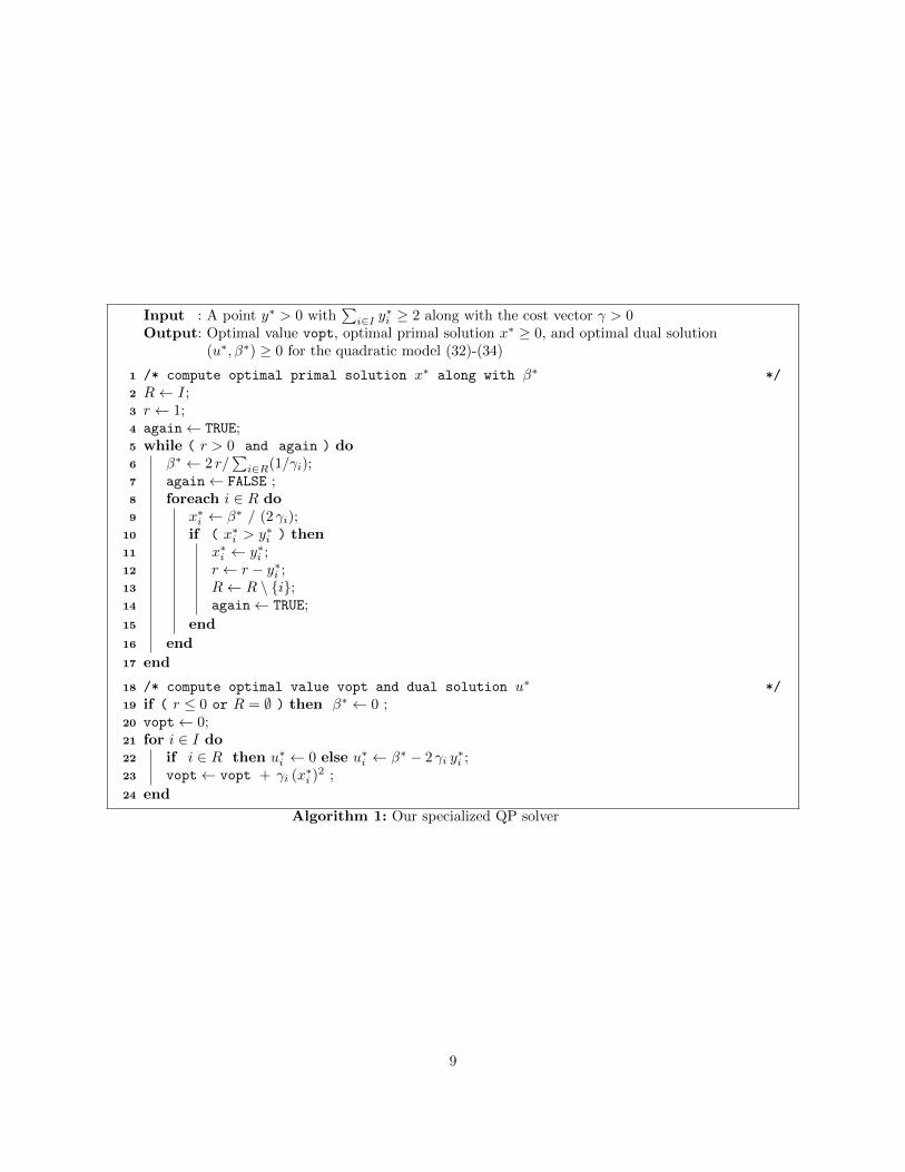
Next, we explain a way of determining optimal primal and associated dual solutions for the QuadraticProgram (QP) given in (32)-(34), without using a general QP solver that would be much slower in oursetting.

Implementing an ad-hoc QP algorithm

Fast algorithms for solving simple QP problems with a knapsack-like constraint and box constraints areavailable in the literature; see, e.g., Hochbaum and Hong [24], Patriksson and Stromberg [44]. In view of itsapplication for GB cut separation, we implemented a basic version of such algorithms, that proved sufficientlyfast (and numerically accurate) for our purposes. To make our results reproducible, we next describe theactual algorithm we used for solving QP problem (32)-(34) and, for the sake of completeness, provide a proofof its correctness.

Let us consider first the following residual problem where the x variables have no upper bounds, R ⊆ Iis a given residual set of facilities, and r ∈ [0, 1] is a given residual request :

min∑i∈R

γix2i (35)∑

i∈Rxi ≥ r. (36)

Let β∗ ≥ 0 be the optimal dual multiplier for inequality (36). It is well known [21]—and easy to proveusing KKT optimality conditions—that an optimal primal-dual pair (x∗, β∗) can be computed as:

β∗ =2r∑

i∈R 1/γi, x∗i =

β∗

2 γifor all i ∈ R. (37)

Our algorithm to solve the quadratic model with bounded variables (32)-(34) derives the optimal solutionby subsequently solving the residual problem (35)-(36) for various values of r and R; see Algorithm 1.

The primal optimal solution x∗ is computed at Steps 1-17 together with β∗ (the latter being the optimaldual multiplier for inequality (33)). To this end, we first set R = I and r = 1 (Steps 2-3) and use (37)to compute the optimal values of x∗i (and β∗) by disregarding their upper bounds in (34). If it happensthat all upper bounds are in fact fulfilled, we are done. Otherwise, for each x∗i > y∗i we truncate x∗i to y∗i(Step 11), update r and R accordingly (Steps 12-13), and repeat. The optimal nonnegative dual variablesu∗i corresponding to (34) are finally defined at Step 22.

To prove the correctness of Algorithm 1, we need the following.

8

Input : A point y∗ > 0 with∑

i∈I y∗i ≥ 2 along with the cost vector γ > 0

Output: Optimal value vopt, optimal primal solution x∗ ≥ 0, and optimal dual solution(u∗, β∗) ≥ 0 for the quadratic model (32)-(34)

1 /* compute optimal primal solution x∗ along with β∗ */

2 R← I;3 r ← 1;4 again← TRUE;5 while ( r > 0 and again ) do6 β∗ ← 2 r/

∑i∈R(1/γi);

7 again← FALSE ;8 foreach i ∈ R do9 x∗i ← β∗ / (2 γi);

10 if ( x∗i > y∗i ) then11 x∗i ← y∗i ;12 r ← r − y∗i ;13 R← R \ {i};14 again← TRUE;

15 end

16 end

17 end

18 /* compute optimal value vopt and dual solution u∗ */

19 if ( r ≤ 0 or R = ∅ ) then β∗ ← 0 ;20 vopt← 0;21 for i ∈ I do22 if i ∈ R then u∗i ← 0 else u∗i ← β∗ − 2 γi y

∗i ;

23 vopt← vopt + γi (x∗i )2 ;

24 end

Algorithm 1: Our specialized QP solver

9

Lemma 3.1. The values β∗ computed at each iteration of Step 6 are strictly monotonically increasing.

Proof. Proof. Let us assume, without loss of generality, that in a given iteration only a single i is removedfrom R. Let β′ and β′′ be the value of β∗ at Step 6 before and after the removal of i from R arising at Step 13,respectively, and let r′ and r′′ be the corresponding values of r. To simplify notation, let us define ρi = 1/γiand d′ =

∑t∈R(1/γt). We have to show that β′′ > β′, where β′ = 2r′/d′ and β′′ = 2(r′ − y∗i )/(d′ − ρi). To

this end, observe that the removal of i from R implies x∗i = β′/(2γi) > y∗i at Step 10, i.e., 2y∗i < β′ρi holds.So

β′′ =2r′ − 2y∗id′ − ρi

>2r′ − β′ρid′ − ρi

= β′2r′/β′ − ρid′ − ρi

= β′d′ − ρid′ − ρi

= β′

as claimed.

Theorem 3.1. Algorithm 1 returns an optimal primal solution x∗ and an optimal dual solution (u∗, β∗) ofproblem (32)-(34).

Proof. Proof. The Lagrangian function for problem (32)-(34) is defined as

L(x, u, β) =∑i∈I

γixi2 + β (1−

∑i∈I

xi) +∑i∈I

ui (xi − y∗i ).

As we have a convex quadratic problem with linear inequalities, all we have to show is that (x∗, u∗, β∗)satisfies the KKT conditions:

∇xL(x∗, u∗, β∗) = 0, (38)

(x∗, u∗, β∗) ≥ 0, (39)∑i∈I

x∗i ≥ 1, (40)

β∗ (1−∑i∈I

x∗i ) = 0, (41)

u∗i (x∗i − y∗i ) = 0 ∀i ∈ I. (42)

Let notation R and r refer to the quantities available at the end of the algorithm. For condition (38), wehave two cases:

• i ∈ R: in this case, u∗i = 0 (Step 22) and x∗i = β∗ / (2γi) (Step 9), hence ∂L(x∗, u∗, β∗)/∂xi =2γix

∗i − β∗ = 0;

• i 6∈ R: in this case, u∗i = β∗ − 2γiy∗i (Step 22) and x∗i = y∗i (Step 11), hence ∂L(x∗, u∗, β∗)/∂xi =

2γix∗i − β∗ + u∗i = 0.

Conditions (39) are obvious except for u∗i and i 6∈ R, when u∗i = β∗ − 2 γi y∗i is defined at Step 22. Let

β′ be the value of β∗ computed at Step 6 at the iteration when i is removed from R at Step 13. Thenx∗i = β′/(2 γi) > y∗i at Step 10. Due to Lemma 3.1, β∗ ≥ β′. By combining this with the rewritten formβ′ > 2 γi y

∗i of the previous inequality, we obtain β∗ > 2 γi y

∗i , from which u∗i ≥ 0 follows.

Also obvious is the complementary slackness condition (41), while (42) derives from u∗i = 0 for all i ∈ R(Step 22) and x∗i = y∗i for all i 6∈ R (Step 11).

Thinning out w variables in the master

In the aim of thinning out irrelevant variables from the master, one can think of replacing all wj ’s by a singlecontinuous variable

wsum =∑j∈J

wj

10

and of aggregating the individual GB cuts for each customer j ∈ J , namely

wj ≥ Φj(y∗) +

∑i∈I

s∗ij(yi − y∗i ), (43)

into a single cumulative GB cut

wsum ≥∑j∈J

Φj(y∗) +

∑i∈I

(∑j∈J

s∗ij)(yi − y∗i ). (44)

In this setting, for each y∗ of the master, one generates at most one violated cut, as opposed to the at most|J | individual cuts that can be generated by keeping the disaggregated variables wj ’s.

In what follows, the model with the individual wj variables will be called the fat model, while the modelwith the single wsum variable will be referred to as the slim model.

The slim model has both pros and cons with respect to the fat one.On the positive side, one does not really need to know the individual wj values associated with a given

y, as the actual solution cost only depends on their sum. By removing the individual wj ’s one can thereforeremove potentially-disturbing information. Moreover, by using the single wsum variable one expects togenerate fewer cuts during the branch-and-cut solution process, hence the LP relaxations of the master willbe smaller in terms of variables and (hopefully) of explicitly-generated GB cuts.

On the negative side, cuts (44) tend to be denser than (43). Moreover, we know that each cumulativecut (44) is just implied (a la Farkas) by their individual counterparts (43), and people working with MIP’shave a Pavlov’s aversion to aggregated formulations. However, in our setting the quality of the lower boundof the master is theoretically the same as they both are the projection on different w-subspaces of the sameformulation, so we are not really losing anything in terms of lower bound if we opt for the cumulative cut.

As it will be discussed in the next section, what matters is in fact the availability of a sound cuttingplane scheme that can effectively produce good lower bounds even when a single cut is generated at eachseparation call. As a matter of fact, at least for quadratic UFL, the slim variant is much more effective thanthe fat one; see Subsection 4.4 for details.

4 The overall solution framework

Once the GB cut separators for both the linear and quadratic cases have been implemented, one has todesign the overall branch-and-cut solution framework for the master MILP problem that separates GB cuts,on the fly, at every branching node.

A natural choice is to use a state-of-the-art commercial MILP solver—we used IBM ILOG Cplex 12.6 inour implementation. Using a state-of-the-art MILP solver does in fact simplify the implementation a lot, asone relies on a very robust and efficient external framework for the parametric solution of the node LP’s,primal heuristics, generation of general MILP cuts, branching, cut pool handling, etc. So, for a quick shotone only has to plug the GB cut separator in the framework, and see how it works. This simple approach isin fact rather effective, as it already allowed us to solve the previously unsolved UFLLIB [25] linear instances2500-10 and 3000-100 in less than 15 minutes (each) on a PC. However, better results—in particular, forthe quadratic case—can be obtained by adding some more ingredients to the basic recipe, as outlined below.

4.1 Numerically accurate GB cuts for the quadratic case

In the quadratic case, when the point y∗ to separate contains zero entries we face theoretical issues in thedefinition of the “perspective costs” γi = ci/y

∗i and hence of the most-violated GB cut. Although in theory

there are elegant ways to cope with the non-differentiability at such points [22], in practice we observed thatthe GB cut becomes numerically unreliable even when y∗i ≈ 0 for some i, hence the risk of producing invalidcuts becomes a real issue.

11

We have therefore implemented a very simple way to encompass the above difficulty which is based onthe fact that, in our separation framework, y∗ is in fact a known quantity—while in the compact MILP(5)-(11) it plays the role of a variable. We introduced a (not too small) internal threshold ε = 10−5 to decidewhether a given y∗ is close enough to zero. Then, for each i ∈ I with y∗i < ε we just resist the temptationand do not apply the perspective strengthening of x2

ij . This means that we replace x2ij ≤ zij yi by x2

ij ≤ zijin (28). In this way we have γi = ci in (32), and the dual variable v∗i will no longer appear in the GB cut asthe new constraint does not depend on y anymore.

Although not strictly required, we also apply the same procedure when y∗i > 1− ε, as in this case whatwe gain from the perspective strengthening is negligible. In a sense, we view the components of y∗ that are“almost integer” as good enough, and we do not believe it is worth to penalize them through the (numericallyrisky) perspective reformulation.

There is a second way to deal with zero entries in y∗, that we call 2 ε trick : just replace each y∗iwith y∗i + 2 ε and apply GB separation to this perturbed point—an idea used by many authors, includingBen-Ameur and Neto [7]. This is mathematically correct because the GB cut we generate is always valid—though its violation with respect to original y∗ is slightly underestimated. Although it may appear naive, thisapproach is rather effective and can significantly improve the overall convergence of the cut loop, as shownin the next subsection. In fact, this idea is closely related to the approach proposed by [20] of “perturbing”perspective inequalities by moving y towards a point “sufficiently inside” the perspective cone—the maindifference being that we face a much simpler situation where y∗ is given, whereas in Grossmann and Lee [20]one needs to treat y as a variable.

4.2 Cut loop stabilization at the root node

This is perhaps the most important ingredient in our recipe. In the MIP community, a lot of attention isgenerally paid to the polyhedral strength of the generated cuts (e.g., the fact of being facet defining), givingfor granted that the external cutting plane loop will follow Kelley’s scheme [27]. According to this scheme, ateach cut loop iteration one generates one or more cuts that are violated by the current (fractional) solutiony∗, adds them to the current relaxation, reoptimizes it and gets a new optimal solution y∗ to be cut at thenext iteration.

However, the convergence behavior of the overall cut loop heavily depends also on the strategy forgenerating the next point to cut. As a matter of fact, the famous ellipsoid method has a very good (at least,theoretically) convergence property, but the single valid cut it generates at each iteration can be very weakin polyhedral terms—actually, it does not even need to be violated but just tight at the separation point.This is because the role of the cut is not to let integer points emerge as vertices of the LP relaxation, butjust to exclude a large subspace from further considerations. Evidently, one can design a sound cutting planeloop even with very weak/dense cuts, provided that a sound cutting plane scheme is adopted.

In the LP relaxation of our MILP master problem, we have a very simple set of feasibility constraints inthe y space (only the 0-1 bounds on the variables and the cardinality condition), and we have to minimizethe convex function

∑i∈I fiyi +

∑j∈J Φj(y). This setting is very close (in fact, identical) to the one arising

in the usual Lagrangian dual minimization (assuming a convex primal problem in maximization form), where“stabilized” approaches such as the bundle method [33] are known to outperform Kelley’s one by a largemargin. Thus, the implementation of stabilized cutting plane at the root node (at least) is expected to beof crucial importance, in particular when a single cut is separated for each point, as it is the case of our slimmaster model with a single wsum variable.

In our current version, we did not implement a real bundle method, but a simple in-out variant verymuch in the spirit of the work of Applegate et al. [1], Ben-Ameur and Neto [7], Fischetti and Salvagnin [13],and [42]. At each cut loop iteration, we have two points in the y space: the optimal solution y∗ of the currentmaster LP (as in Kelley’s method), and a stabilizing point y which is initialized to y = (1, . . . , 1).

At each step, we move y halfway towards y∗ by setting y = 12 (y + y∗) and then apply our GB separator

to the “intermediate point”λ y∗ + (1− λ) y + δ(1, . . . , 1).

12

0 0.1 1 10 100 1000time (sec.s)

2000

4000

6000

8000

10000

12000

low

er b

ound

ImportImportImport

inout Kelley+

Kelley

* nc = 748

* nc = 55,004

nc = 10,757

nc = 3,257

nc = 57,507

fat model

0 0.1 1 10 100 1000time (sec.s)

2000

4000

6000

8000

10000

12000

low

er b

ound

Kelley+inout

slim model

Kelley

*nc = 4

*nc = 1,496

nc = 169

nc = 1,221

nc = 2,703

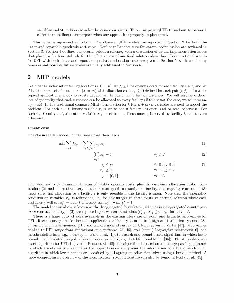
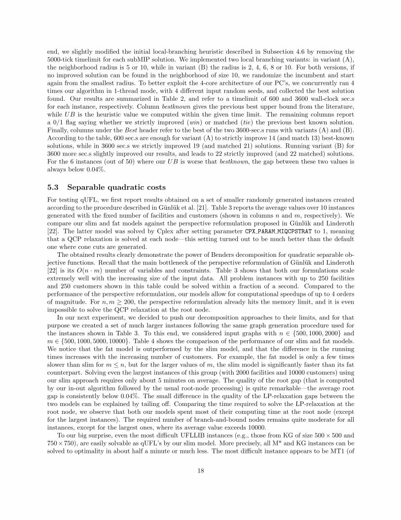
Figure 1: Performance of three cut loop strategies with fat (left subfigure) and slim (right) models on thesample Koerkel-Ghosh [29] instance gs250a-1 with n = m = 250 (quadratic costs). We compare standardKelley, Kelley+ (i.e., Kelley enhanced by the 2 ε trick), and our inout scheme. Label *nc reports thenumber of active cuts at the end of the root node. Time axis given in logarithmic scale.

Parameters λ ∈ (0, 1] and δ ≥ 0 are initially set to 0.2 and 2 ε, meaning that we initially consider pointsvery close to the current stabilizer. The generated GB cuts (in the (y, w) space) are statically added tothe current LP. After 5 consecutive iterations in which the LP bound does not improve, parameter λ isreset to 1 and the cut loop continues. After 5 more consecutive iterations with no LP bound improvement,parameter δ is reset to 0 (so we are back to Kelley’s scheme). After 5 more consecutive iterations withoutimprovement, the procedure is aborted and all cuts with a positive slack in the final LP are removed. Tospeedup computation, slack cuts from the current LP are also removed at every 5-th iteration.

According to our computational experience, the above cut loop is very effective for the slim model whereGB separation returns at most one single cut at each call, in particular for the quadratic case where thedifference with respect to the straightforward Kelley’s is striking.

In Figure 1 we plot the behavior of three cut loop strategies (single-thread run) on a sample instance withquadratic costs, namely, the Koerkel-Ghosh [29] instance gs250a-1 with 250 locations and 250 clients whoseoptimal value is 12,633.858555. All methods are based on exactly the same GB separator, and only differon the policy to select the point y∗ to cut at each iteration. Kelley refers to the standard approach, whileKelley+ adopts the 2 ε trick thus slightly perturbing the point to cut before invoking the GB separator.Finally, inout refers to our simple scheme using the stabilizer y as described above. Note that in thehorizontal axis we had to use a logarithmic scale due to the dramatically different performance of the threemethods. We consider both the fat and the slim models.

When the fat model is used, Kelley has a very poor performance: we stopped it after 15,000 sec.s (stillat the root node) with a lower bound of just 1,781.035992, and more than 100,000 cuts generated. Kelley+has a much better performance than Kelley, showing the effectiveness of the 2 ε trick. Its root node takes948.86 sec.s to generate 55,004 cuts, and produces a very tight bound of 12,633.118973. Enumeration to prove

13

optimality takes 48 branching nodes and is completed at time 978.53. The performance of inout is howeverdramatically better: its root node requires just 0.19 sec.s and produces a lower bound of 12,633.280331 with748 cuts, while enumeration ends at time 0.41 after 6 nodes.

The performance differences are even more striking for the slim model. Kelley has again a very poorperformance: we stopped it after 500 nodes (8,208.67 sec.s) with a lower bound of 1,875.111861 and 6,037cuts generated. Kelley+ has a better performance: its root node takes 98.27 sec.s to generate 1,496 cuts,and produces a bound of 12,632.092567; enumeration to prove optimality takes 44 branching nodes and iscompleted at time 100.66. The performance of inout is so good that its plot is barely visible in the figure:its root node requires 0.04 sec.s and produces a lower bound of 12,633.101453 after adding only 4 cuts, whileenumeration ends at time 0.06 after 11 nodes.

In our implementation, the stabilized cut loop is implemented as a separate preprocessing function tobe applied before starting the branch-and-cut algorithm, hence it only affects the root-node formulationand lower bound. For the reasons explained below, the classical Kelley’s cut loop is instead applied at thenon-root nodes.

4.3 Cut loop along the tree

At each branch-decision node, the MILP framework automatically invokes our GB cut separator (within aso-called user cut callback) just before branching, after having solved the current node LP and havingadded possible violated cuts from its internal cut pool and/or generated by internal procedures. The currentLP solution (y∗, w∗) is passed to our GB cut separator, that possibly returns one or more violated cuts.

The violated GB cuts returned by our separation procedure, if any, are added to the internal cut pooland eventually to the current-node LP, which is reoptimized to provide a new solution (y∗, w∗), and theapproach is iterated. Thus, the solver natively implements the Kelley cutting plane scheme, which is notnecessarily the best possible option for weak/dense cuts. Implementing a more clever cut loop within Cplexis however not immediate, so we preferred to keep the default Kelley’s scheme within the MILP solver.

To avoid tailing off, we imposed a limit of 20 consecutive cut loop iterations for each node (2,000 for theroot node).

Although globally valid, at each node all generated cuts are added as “local cuts” as this allows Cplex toremove more cuts from its internal pool—this turned out to be mainly useful in the case with linear costs,where lots of cuts are generated.

4.4 Slim or fat model?

According to our tests, the slim version with wsum variable is a clear winner for the quadratic case. In ourview, this is due to two main reasons. First of all, the stabilized cut loop of the previous subsection performsvery well for the quadratic case, and allows us to compute a really tight root-node lower bound with a verysmall LP with just n + 1 variables and very few cuts. Second, the lower bound is so tight that very fewbranching nodes are generated, so the fact that the poor Kelley’s cut loop is applied at the non-root nodesis not really an issue.

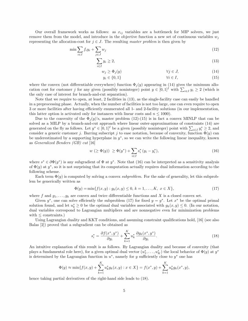
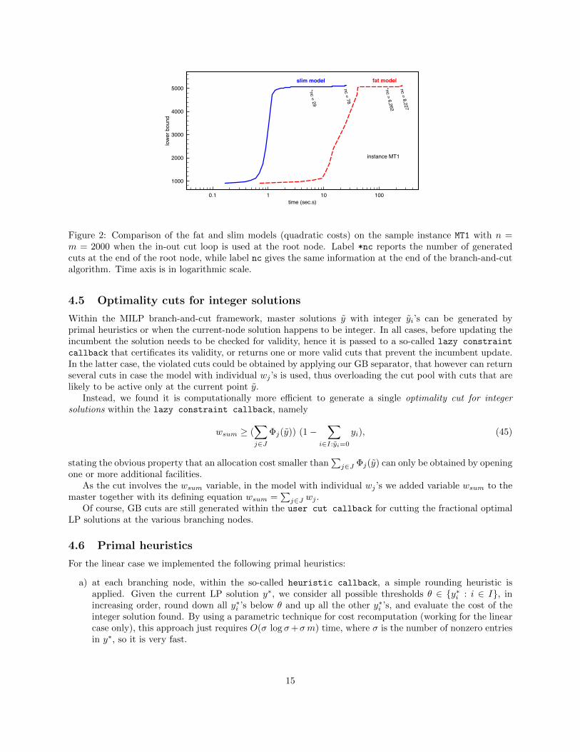
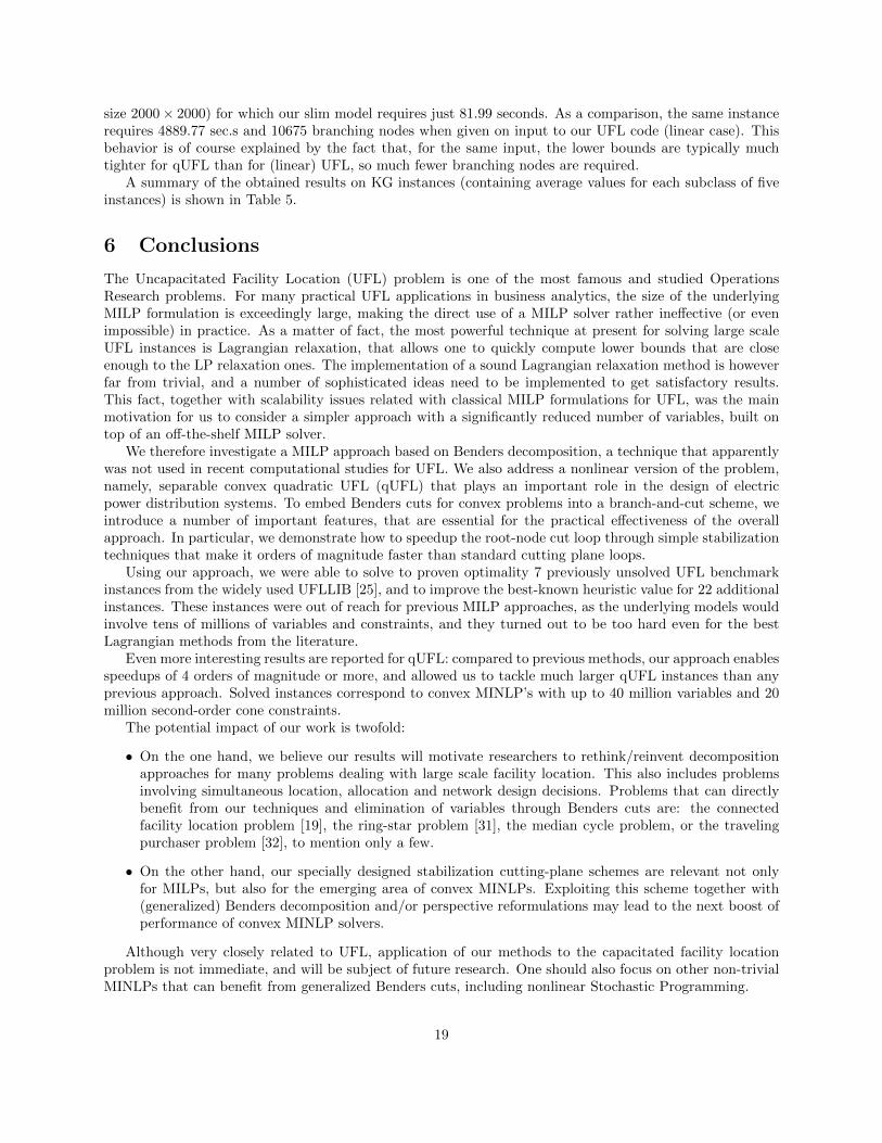
In Figure 2 we plot the behavior of the fat and slim models on the sample instance MT1 with n = m = 2000and quadratic costs and 4-thread run. At the root node, our in-out cut loop scheme is adopted in both cases.Note that times are reported in logarithmic scale.

On the contrary, for the linear case the fat version with the individual wj ’s variables turns out to be muchbetter. A main reason is that the root-node lower bound is not really tight, so a considerable amount ofnodes are enumerated anyway. So Kelley’s approach prevents an effective recomputation of the node boundswhen a single cut at the time is generated (wsum version), while it performs reasonably well when severalcuts are generated (version with individual wj ’s).

14

0.1 1 10 100time (sec.s)

1000

2000

3000

4000

5000

low

er b

ound

fat modelslim model

*nc = 29

nc = 78

*nc = 6,262

nc = 8,227

instance MT1

Figure 2: Comparison of the fat and slim models (quadratic costs) on the sample instance MT1 with n =m = 2000 when the in-out cut loop is used at the root node. Label *nc reports the number of generatedcuts at the end of the root node, while label nc gives the same information at the end of the branch-and-cutalgorithm. Time axis is in logarithmic scale.

4.5 Optimality cuts for integer solutions

Within the MILP branch-and-cut framework, master solutions y with integer yi’s can be generated byprimal heuristics or when the current-node solution happens to be integer. In all cases, before updating theincumbent the solution needs to be checked for validity, hence it is passed to a so-called lazy constraint

callback that certificates its validity, or returns one or more valid cuts that prevent the incumbent update.In the latter case, the violated cuts could be obtained by applying our GB separator, that however can returnseveral cuts in case the model with individual wj ’s is used, thus overloading the cut pool with cuts that arelikely to be active only at the current point y.

Instead, we found it is computationally more efficient to generate a single optimality cut for integersolutions within the lazy constraint callback, namely

wsum ≥ (∑j∈J

Φj(y)) (1−∑

i∈I:yi=0

yi), (45)

stating the obvious property that an allocation cost smaller than∑

j∈J Φj(y) can only be obtained by openingone or more additional facilities.

As the cut involves the wsum variable, in the model with individual wj ’s we added variable wsum to themaster together with its defining equation wsum =

∑j∈J wj .

Of course, GB cuts are still generated within the user cut callback for cutting the fractional optimalLP solutions at the various branching nodes.

4.6 Primal heuristics

For the linear case we implemented the following primal heuristics:

a) at each branching node, within the so-called heuristic callback, a simple rounding heuristic isapplied. Given the current LP solution y∗, we consider all possible thresholds θ ∈ {y∗i : i ∈ I}, inincreasing order, round down all y∗i ’s below θ and up all the other y∗i ’s, and evaluate the cost of theinteger solution found. By using a parametric technique for cost recomputation (working for the linearcase only), this approach just requires O(σ log σ+σm) time, where σ is the number of nonzero entriesin y∗, so it is very fast.

15

b) local branching: right after the cut loop at the root node, we apply the local branching heuristic [11]with neighborhood radius starting from k = 5 and then increased to 10, using a small time limit foreach call (5000 ticks, corresponding to approximately 5 sec.s on our hardware). The heuristic is abortedwhen no improved solution is found in the neighborhood of size 10.

c) proximity search: right after local branching, we apply proximity search heuristic [12] until no improvedsolution can be found within the small time limit imposed for each call (5000 ticks).

As to the quadratic case, according to our experience the performance of our method is so good that thereis no really need to design specific primal heuristics. So for the quadratic case only the rounding heuristica) above is applied, with a fixed threshold θ = max{y∗i : i ∈ I} − 0.2.

4.7 Numerical tolerances and cut validity

In our implementation, we were very conservative and used very small tolerances for numerical and integralitytests. To be specific, we set Cplex’s integrality tolerance CPX PARAM EPINT to 0, and the optimality/violationtolerances CPX PARAM EPGAP and CPX PARAM EPRHS to 10−9. Our own internal numerical tolerance was setto 10−9 as well.

To assert the validity of the GB cuts we generate in our code, we implemented the following check inthe spirit of Margot’s proposal [38]. At the end of the run (or at the time limit), we fix all (binary andcontinuous) variables to their value in the incumbent solution, and enter a cut loop where (1) we apply ourGB cut separator to a point y∗ obtained from the incumbent by a small random perturbation (applied to80% random entries) ranging from 10−9 to 10−1, (2) we statically add the generated cuts to the currentMILP, and (3) we optimize the MILP to verify its feasibility. If the current MILP becomes infeasible, wewrite down the current model in a file for further analysis and report a failure, otherwise we repeat for 10,000times. The above check was applied extensively during the development of our code. Although it was notdesigned to cover all possible cut failures, the check helped us in detecting and correcting some toleranceissues present in the earlier versions.

5 Computational results

In this section we report on our computational experience on a subset of most difficult instances for UFL. Asto qUFL, we consider instances used in the previous literature, extended by a family of much larger instancesthat cannot be approached by existing methods—mainly due to the fact that the underlying models wouldconsist of millions of variables and constraints. The computational study is conducted on a cluster of identicalmachines each consisting of an Intel Xeon E3-1220V2 CPU running at 3.10 GHz, with 16GB of RAM each.Reported times are wall-clock seconds and refer to 4-thread runs.

We report computational results with basic parameter settings, without tuning our code with respect toproximity search and/or local branching parameters that could theoretically further improve the obtainedresults.

5.1 Benchmark instances

The set of UFL benchmark instances used in this paper stems from the UFLLIB [25], which is a well-established library of instances for capacitated and uncapacitated facility location problems. The libraryis a diverse collection of bipartite graphs, some of them being just small and easily solvable cases. In ourstudy on UFL, we focus on a subset instances from UFLLIB representing the most challenging ones evenfor the most recent state-of-the-art approaches, like the ones proposed by Beltran-Royo et al. [6], Letchfordand Miller [35] and Posta et al. [45]. These are the randomly generated instances M* proposed in Kraticaet al. [30], and the KG instances proposed in Ghosh [18], Korkel [29]. Instances M* are of size 100× 100 upto 2000 × 2000, whereas the KG instances can be divided into three groups, with n = m ∈ {250, 500, 750}.Within each KG group, there are two classes, symmetric and asymmetric ones, denoted by gs* and ga*,

16

respectively. Additionally, each class contains three subclasses, “a”, “b” and “c”, representing different costsettings: in “a”, allocation costs are an order of magnitude higher than the facility opening costs; in “b”,these costs are of the same order; and in “c”, facility opening costs are an order of magnitude higher thanthe allocation costs. As we will report below, these differences in the cost structure significantly influencetheir computationally difficulty.

For testing the impact of Benders decomposition to the separable quadratic case, we consider two familiesof benchmark instances: (1) UFLLIB instances mentioned above plus the instances from the ORLIB [5] (withoriginal allocation costs equal to 0 being replaced by 10−5), and (2) randomly generated instances used inprevious computational studies by Bonami et al. [8], Gunluk et al. [21] and Gunluk and Linderoth [22].The latter instances are randomly generated graphs with potential facility and customer locations beingplaced uniformly at random within a unit square, with allocation costs calculated as the Euclidean distancemultiplied by a factor of 50, and facility opening costs generated uniformly in [1, 100]. Tables shown in thissection report the total running time in wall-clock seconds (t[s]), the time needed to solve the LP-relaxationat the root node (troot[s]), the total number of branch and bound nodes needed to prove the optimality(nodes) and the percentage gap at the root node (gr[%], computed with respect to the optimal solutionvalue) and the dual bound at the root node (rootbound).

5.2 Linear costs

For solving UFL with linear costs, we opted for the branch-up-first setting (Cplex’s parameter CPX PARAM BRDIR

set to 1), as this tends to produce branching trees with fewer open nodes—hence reducing the overhead in-curred when writing the node files automatically generated by Cplex when the branching tree becomes solarge that cannot be stored into the available RAM (16GB in our runs).

Table 1 summarizes results for the previously unsolved UFL instances for which we were able to prove op-timality. In total, optimal solutions are provided for seven previously unsolved instances. Column bestknowngives the best known solution value from the literature, while opt gives the optimal solution value.

Two of them belong to the benchmark set of 18 instances proposed by [3]. The semi-Lagrangian approachby Beltran-Royo et al. [6] solved 16 of them, whereas the approach by Posta et al. [45] managed to solveonly 8 of these 16. We provide the optimal values for the remaining two unsolved instances, namely, 2500-10and 3000-100, of size 2500× 2500 and 3000× 3000, respectively.

Concerning the 30 instances of size 250 × 250 proposed by Korkel [29], we could solve all of them toproven optimality. 27 such instances were already solved by Posta et al. [45], and an additional one (ga250a-1) was solved by Beltran-Royo et al. [6]. Therefore we only report in Table 1 the optimal value for the twopreviously unsolved instances, namely, ga250a-3 and ga250a-5. Among the KG instances of size 500 × 500,optimal values were known only for 7 (out of 10) instances of the subclass g∗500c∗. We were able to provethe optimality for all the instances in this subclass, including the three missing ones (ga500c-5, gs500c-3,and gs500c-5).

Table 1: Previously unsolved UFL instances solved to optimality using our approach (linear costs).

inst. bestknown opt t[s] rootbound troot[s] gr[%] nodes

2500-10 3101800 3099907 824.76 3097480.189279 104.67 0.08 13623000-100 1602335 1602154 225.25 1601733.816607 82.67 0.03 441ga250a-3 257985 257953 493.49 257554.773407 12.77 0.15 200184ga250a-5 258225 258190 585.93 257790.245068 9.65 0.15 229446ga500c-5 621313 621313 9226.86 601500.282332 12.31 3.19 195191gs500c-3 621204 621204 11448.19 601980.526816 13.44 3.09 194657gs500c-5 623180 623180 26828.91 603115.401650 14.20 3.22 270147

The 50 KG instances of subclasses g∗500a, g∗500b, g∗750∗ still remain out of reach for existing exactmethods. However, we managed to improve the best known upper bounds for 22 of these instances. To this

17

end, we slightly modified the initial local-branching heuristic described in Subsection 4.6 by removing the5000-tick timelimit for each subMIP solution. We implemented two local branching variants: in variant (A),the neighborhood radius is 5 or 10, while in variant (B) the radius is 2, 4, 6, 8 or 10. For both versions, ifno improved solution can be found in the neighborhood of size 10, we randomize the incumbent and startagain from the smallest radius. To better exploit the 4-core architecture of our PC’s, we concurrently ran 4times our algorithm in 1-thread mode, with 4 different input random seeds, and collected the best solutionfound. Our results are summarized in Table 2, and refer to a timelimit of 600 and 3600 wall-clock sec.sfor each instance, respectively. Column bestknown gives the previous best upper bound from the literature,while UB is the heuristic value we computed within the given time limit. The remaining columns reporta 0/1 flag saying whether we strictly improved (win) or matched (tie) the previous best known solution.Finally, columns under the Best header refer to the best of the two 3600-sec.s runs with variants (A) and (B).According to the table, 600 sec.s are enough for variant (A) to strictly improve 14 (and match 13) best-knownsolutions, while in 3600 sec.s we strictly improved 19 (and matched 21) solutions. Running variant (B) for3600 more sec.s slightly improved our results, and leads to 22 strictly improved (and 22 matched) solutions.For the 6 instances (out of 50) where our UB is worse that bestknown, the gap between these two values isalways below 0.04%.

5.3 Separable quadratic costs

For testing qUFL, we first report results obtained on a set of smaller randomly generated instances createdaccording to the procedure described in Gunluk et al. [21]. Table 3 reports the average values over 10 instancesgenerated with the fixed number of facilities and customers (shown in columns n and m, respectively). Wecompare our slim and fat models against the perspective reformulation proposed in Gunluk and Linderoth[22]. The latter model was solved by Cplex after setting parameter CPX PARAM MIQCPSTRAT to 1, meaningthat a QCP relaxation is solved at each node—this setting turned out to be much better than the defaultone where cone cuts are generated.

The obtained results clearly demonstrate the power of Benders decomposition for quadratic separable ob-jective functions. Recall that the main bottleneck of the perspective reformulation of Gunluk and Linderoth[22] is its O(n · m) number of variables and constraints. Table 3 shows that both our formulations scaleextremely well with the increasing size of the input data. All problem instances with up to 250 facilitiesand 250 customers shown in this table could be solved within a fraction of a second. Compared to theperformance of the perspective reformulation, our models allow for computational speedups of up to 4 ordersof magnitude. For n,m ≥ 200, the perspective reformulation already hits the memory limit, and it is evenimpossible to solve the QCP relaxation at the root node.

In our next experiment, we decided to push our decomposition approaches to their limits, and for thatpurpose we created a set of much larger instances following the same graph generation procedure used forthe instances shown in Table 3. To this end, we considered input graphs with n ∈ {500, 1000, 2000} andm ∈ {500, 1000, 5000, 10000}. Table 4 shows the comparison of the performance of our slim and fat models.We notice that the fat model is outperformed by the slim model, and that the difference in the runningtimes increases with the increasing number of customers. For example, the fat model is only a few timesslower than slim for m ≤ n, but for the larger values of m, the slim model is significantly faster than its fatcounterpart. Solving even the largest instances of this group (with 2000 facilities and 10000 customers) usingour slim approach requires only about 5 minutes on average. The quality of the root gap (that is computedby our in-out algorithm followed by the usual root-node processing) is quite remarkable—the average rootgap is consistently below 0.04%. The small difference in the quality of the LP-relaxation gaps between thetwo models can be explained by tailing off. Comparing the time required to solve the LP-relaxation at theroot node, we observe that both our models spent most of their computing time at the root node (exceptfor the largest instances). The required number of branch-and-bound nodes remains quite moderate for allinstances, except for the largest ones, where its average value exceeds 10000.

To our big surprise, even the most difficult UFLLIB instances (e.g., those from KG of size 500× 500 and750×750), are easily solvable as qUFL’s by our slim model. More precisely, all M* and KG instances can besolved to optimality in about half a minute or much less. The most difficult instance appears to be MT1 (of

18

size 2000× 2000) for which our slim model requires just 81.99 seconds. As a comparison, the same instancerequires 4889.77 sec.s and 10675 branching nodes when given on input to our UFL code (linear case). Thisbehavior is of course explained by the fact that, for the same input, the lower bounds are typically muchtighter for qUFL than for (linear) UFL, so much fewer branching nodes are required.

A summary of the obtained results on KG instances (containing average values for each subclass of fiveinstances) is shown in Table 5.

6 Conclusions

The Uncapacitated Facility Location (UFL) problem is one of the most famous and studied OperationsResearch problems. For many practical UFL applications in business analytics, the size of the underlyingMILP formulation is exceedingly large, making the direct use of a MILP solver rather ineffective (or evenimpossible) in practice. As a matter of fact, the most powerful technique at present for solving large scaleUFL instances is Lagrangian relaxation, that allows one to quickly compute lower bounds that are closeenough to the LP relaxation ones. The implementation of a sound Lagrangian relaxation method is howeverfar from trivial, and a number of sophisticated ideas need to be implemented to get satisfactory results.This fact, together with scalability issues related with classical MILP formulations for UFL, was the mainmotivation for us to consider a simpler approach with a significantly reduced number of variables, built ontop of an off-the-shelf MILP solver.

We therefore investigate a MILP approach based on Benders decomposition, a technique that apparentlywas not used in recent computational studies for UFL. We also address a nonlinear version of the problem,namely, separable convex quadratic UFL (qUFL) that plays an important role in the design of electricpower distribution systems. To embed Benders cuts for convex problems into a branch-and-cut scheme, weintroduce a number of important features, that are essential for the practical effectiveness of the overallapproach. In particular, we demonstrate how to speedup the root-node cut loop through simple stabilizationtechniques that make it orders of magnitude faster than standard cutting plane loops.

Using our approach, we were able to solve to proven optimality 7 previously unsolved UFL benchmarkinstances from the widely used UFLLIB [25], and to improve the best-known heuristic value for 22 additionalinstances. These instances were out of reach for previous MILP approaches, as the underlying models wouldinvolve tens of millions of variables and constraints, and they turned out to be too hard even for the bestLagrangian methods from the literature.

Even more interesting results are reported for qUFL: compared to previous methods, our approach enablesspeedups of 4 orders of magnitude or more, and allowed us to tackle much larger qUFL instances than anyprevious approach. Solved instances correspond to convex MINLP’s with up to 40 million variables and 20million second-order cone constraints.

The potential impact of our work is twofold:

• On the one hand, we believe our results will motivate researchers to rethink/reinvent decompositionapproaches for many problems dealing with large scale facility location. This also includes problemsinvolving simultaneous location, allocation and network design decisions. Problems that can directlybenefit from our techniques and elimination of variables through Benders cuts are: the connectedfacility location problem [19], the ring-star problem [31], the median cycle problem, or the travelingpurchaser problem [32], to mention only a few.

• On the other hand, our specially designed stabilization cutting-plane schemes are relevant not onlyfor MILPs, but also for the emerging area of convex MINLPs. Exploiting this scheme together with(generalized) Benders decomposition and/or perspective reformulations may lead to the next boost ofperformance of convex MINLP solvers.

Although very closely related to UFL, application of our methods to the capacitated facility locationproblem is not immediate, and will be subject of future research. One should also focus on other non-trivialMINLPs that can benefit from generalized Benders cuts, including nonlinear Stochastic Programming.

19

Acknowledgement

This research was funded by the Vienna Science and Technology Fund (WWTF) through project ICT15-014. The first author was also supported by the University of Padova (Progetto di Ateneo “Exploitingrandomness in Mixed Integer Linear Programming”), and by MiUR, Italy (PRIN project “Mixed-IntegerNonlinear Optimization: Approaches and Applications”). The work of I. Ljubic and M. Sinnl was alsosupported by the Austrian Research Fund (FWF, Project P 26755-N19), while that of the last author wasalso supported by an STSM Grant from COST Action TD1207. Thanks are also due to two anonymousreferees for their helpful comments.

References

[1] Applegate, D., R. Bixby, V. Chvatal, W. Cook. 2006. The traveling salesman problem: a computationalstudy . Princeton University Press, Princeton, NJ.

[2] Balas, E. 1971. A duality theorem and an algorithm for (mixed-) integer nonlinear programming. LinearAlgebra Appl. 4(4) 341–352.

[3] Barahona, F., F. Chudak. 2000. Solving large scale uncapacitated facility location problems. P. Parda-los, ed., Approximation and Complexity in Numerical Optimization, Nonconvex Optimization and ItsApplications, vol. 42. Springer US, 48–62.

[4] Basu, S., M. Sharma, P. Ghosh. 2015. Metaheuristic applications on discrete facility location problems:a survey. OPSEARCH 52(3) 530–561.

[5] Beasley, J. E. 1990. OR-Library: Distributing Test Problems by Electronic Mail. J. Oper. Res. Soc.41(11) 1069–1072.

[6] Beltran-Royo, C., J.-P. Vial, A. Alonso-Ayuso. 2012. Semi-Lagrangian relaxation applied to the unca-pacitated facility location problem. Comput. Optim. Appl. 51(1) 387–409.

[7] Ben-Ameur, W., J. Neto. 2007. Acceleration of cutting-plane and column generation algorithms: Ap-plications to network design. Networks 49(1) 3–17.

[8] Bonami, P., M. Kilinc, J. Linderoth. 2012. Algorithms and software for convex mixed integer nonlinearprograms. J. Lee, S. Leyffer, eds., Mixed Integer Nonlinear Programming , vol. 154. Springer, 1–39.

[9] Cornuejols, G., G.L. Nemhauser, L.A. Wolsey. 1980. A canonical representation of simple plant locationproblems and its applications. SIAM J. Algebr. Discr. Meth. 1(3) 261–272.

[10] D’Ambrosio, C., J. Lee, A. Wachter. 2009. A global-optimization algorithm for mixed-integer nonlinearprograms having separable non-convexity. A. Fiat, P. Sanders, eds., Algorithms - ESA 2009 , LectureNotes in Computer Science, vol. 5757. Springer Berlin Heidelberg, 107–118.

[11] Fischetti, M., A. Lodi. 2003. Local branching. Math. Programming 98(1-3) 23–47.

[12] Fischetti, M., M. Monaci. 2014. Proximity search for 0-1 mixed-integer convex programming. J. Heuris-tics 20(6) 709–731.

[13] Fischetti, M., D. Salvagnin. 2010. An in-out approach to disjunctive optimization. A. Lodi, M. Milano,P. Toth, eds., Integration of AI and OR Techniques in Constraint Programming for CombinatorialOptimization Problems, Lecture Notes in Computer Science, vol. 6140. Springer Berlin Heidelberg,136–140.

[14] Frangioni, A., C. Gentile. 2006. Perspective cuts for a class of convex 0-1 mixed integer programs. Math.Programming 106(2) 225–236.

20

[15] Friberg, H. A. 2014. CBLIB 2014: A benchmark library for conic mixed-integer and continuous opti-mization. Optimization Online URL http://cblib.zib.de/.

[16] Geoffrion, A. 1972. Generalized Benders Decomposition. J. Optim. Theory Appl. 10 237–260.

[17] Georgilakis, P.S., N.D. Hatziargyriou. 2013. Optimal distributed generation placement in power distri-bution networks: Models, methods, and future research. IEEE Trans. Pow. Sys. 28(3) 3420–3428.

[18] Ghosh, D. 2003. Neighborhood search heuristics for the uncapacitated facility location problem. Eur.J. Oper. Res. 150(1) 150–162.

[19] Gollowitzer, S., I. Ljubic. 2011. MIP models for connected facility location: A theoretical and compu-tational study. Comput. Oper. Res. 38(2) 435–449.

[20] Grossmann, I. E., S. Lee. 2003. Generalized convex disjunctive programming: Nonlinear convex hullrelaxation. Comput. Optim. Appl. 26(1) 83–100.

[21] Gunluk, O., J. Lee, R. Weismantel. 2007. MINLP strenghtening for separable convex quadratictransportation-cost UFL. Tech. Rep. RC24213 (W0703-042), IBM Research Division.

[22] Gunluk, O., J. Linderoth. 2012. Perspective reformulation and applications. J. Lee, S. Leyffer, eds.,Mixed Integer Nonlinear Programming . Springer, 61–92.

[23] Hijazi, H., P. Bonami, A. Ouorou. 2014. An outer-inner approximation for separable mixed-integernonlinear programs. INFORMS J. Comput. 26(1) 31–44.

[24] Hochbaum, D. S, S.-P. Hong. 1995. About strongly polynomial time algorithms for quadratic optimiza-tion over submodular constraints. Math. Programming 69(1-3) 269–309.

[25] Hoefer, M. 2006. UFLLIB: A collection of benchmark instances for the Uncapacitated Facility Lo-cation Problem. URL http://resources.mpi-inf.mpg.de/departments/d1/projects/benchmarks/

UflLib/.

[26] Ke, Q., E. Ferrara, F. Radicchi, A. Flammini. 2015. Defining and identifying Sleeping Beauties inscience. PNAS 112(24) 7426–7431.

[27] Kelley, J. E. Jr. 1960. The cutting-plane method for solving convex programs. Journal of the Societyfor Industrial and Applied Mathematics 8(4) 703–712.

[28] Klose, A., A. Drexl. 2005. Facility location models for distribution system design. Eur. J. Oper. Res.162(1) 4–29.

[29] Korkel, M. 1989. On the exact solution of large-scale simple plant location problems. Eur. J. Oper.Res. 39(2) 157–173.

[30] Kratica, J., D. Tosic, V. Filipovic, I. Ljubic. 2001. Solving the simple plant location problem by geneticalgorithm. RAIRO-Oper. Res. 35(01) 127–142.

[31] Labbe, M., G. Laporte, I. Rodrıguez-Martın, J. J. Salazar-Gonzalez. 2004. The ring star problem:Polyhedral analysis and exact algorithm. Networks 43(3) 177–189.

[32] Laporte, G., J. Riera Ledesma, J.J. Salazar Gonzalez. 2003. A branch-and-cut algorithm for the undi-rected traveling purchaser problem. Oper. Res. 51(66) 940–951.

[33] Lemarechal, C., A. Nemirovskii, Y. Nesterov. 1995. New variants of bundle methods. Math. Program-ming 69(1-3) 111–147.

[34] Letchford, A., S. Miller. 2012. Fast bounding procedures for large instances of the simple plant locationproblem. Comput. Oper. Res. 39(5) 985–990.

21

[35] Letchford, A., S. Miller. 2014. An aggressive reduction scheme for the simple plant location problem.Eur. J. Oper. Res. 234(3) 674–682.

[36] Li, S. 2013. A 1.488 approximation algorithm for the uncapacitated facility location problem. Infor-mation and Computation 222 45–58. 38th International Colloquium on Automata, Languages andProgramming (ICALP 2011).

[37] Magnanti, T. L., R. T. Wong. 1981. Accelerating Benders decomposition: Algorithmic enhancementand model selection criteria. Oper. Res. 29(3) 464–484.

[38] Margot, F. 2009. Testing cut generators for mixed-integer linear programming. Math. ProgrammingComput. 1(1) 69–95.

[39] Martello, Toth. 1990. Knapsack Problems: Algorithms and Computer Implementations. Wiley, NewYork.

[40] Meisel, S., D. Mattfeld. 2010. Synergies of operations research and data mining. Eur. J. Oper. Res.206(1) 1–10.

[41] Melo, M.T., S. Nickel, F. Saldanha da Gama. 2009. Facility location and supply chain management –a review. Eur. J. Oper. Res. 196(2) 401–412.

[42] Naoum-Sawaya, J., S. Elhedhli. 2013. An interior-point Benders based branch-and-cut algorithm formixed integer programs. Ann. Oper. Res. 210(1) 33–55.

[43] Olafsson, S., X. Li, S. Wu. 2008. Operations research and data mining. Eur. J. Oper. Res. 187(3)1429–1448.

[44] Patriksson, M., C. Stromberg. 2015. Algorithms for the continuous nonlinear resource allocationproblem—new implementations and numerical studies. Eur. J. Oper. Res. 243(3) 703–722.

[45] Posta, M., J. A. Ferland, P. Michelon. 2014. An exact cooperative method for the uncapacitated facilitylocation problem. Math. Programming Comput. 6(3) 199–231.

[46] Shmoys, D. B., E. Tardos, K. Aardal. 1997. Approximation algorithms for facility location problems.Proceedings of the twenty-ninth annual ACM symposium on theory of computing . ACM, 265–274.

[47] Verter, V. 2011. Uncapacitated and capacitated facility location problems. H. A. Eiselt, V. Marianov,eds., Foundations of Location Analysis, International Series in Operations Research & ManagementScience, vol. 155. Springer, 25–37.

22

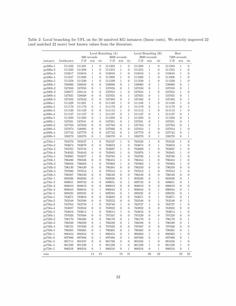
Table 2: Local branching for UFL on the 50 unsolved KG instances (linear costs). We strictly improved 22(and matched 22 more) best known values from the literature.

Local Branching (A) Local Branching (B) Best600 seconds 3600 seconds 3600 seconds 7200 seconds

instance bestknown UB win tie UB win tie UB win tie UB win tie

ga500a-1 511422 511401 1 0 511383 1 0 511388 1 0 511383 1 0ga500a-2 511333 511288 1 0 511255 1 0 511255 1 0 511255 1 0ga500a-3 510817 510810 1 0 510810 1 0 510810 1 0 510810 1 0ga500a-4 511047 511008 1 0 511008 1 0 511008 1 0 511008 1 0ga500a-5 511258 511239 1 0 511239 1 0 511239 1 0 511239 1 0ga500b-1 538060 538656 0 0 538060 0 1 538060 0 1 538060 0 1ga500b-2 537850 537850 0 1 537850 0 1 537850 0 1 537850 0 1ga500b-3 538077 538144 0 0 537924 1 0 537924 1 0 537924 1 0ga500b-4 537925 538038 0 0 537925 0 1 537925 0 1 537925 0 1ga500b-5 537482 537642 0 0 537482 0 1 537482 0 1 537482 0 1gs500a-1 511229 511201 1 0 511188 1 0 511188 1 0 511188 1 0gs500a-2 511179 511179 0 1 511179 0 1 511179 0 1 511179 0 1gs500a-3 511120 511129 0 0 511112 1 0 511112 1 0 511112 1 0gs500a-4 511137 511137 0 1 511137 0 1 511137 0 1 511137 0 1gs500a-5 511293 511293 0 1 511293 0 1 511293 0 1 511293 0 1gs500b-1 537931 537941 0 0 537931 0 1 537931 0 1 537931 0 1gs500b-2 537763 537823 0 0 537763 0 1 537763 0 1 537763 0 1gs500b-3 537874 538095 0 0 537926 0 0 537854 1 0 537854 1 0gs500b-4 537742 537779 0 0 537742 0 1 537779 0 0 537742 0 1gs500b-5 538270 538270 0 1 538270 0 1 538270 0 1 538270 0 1

ga750a-1 763576 763537 1 0 763537 1 0 763528 1 0 763528 1 0ga750a-2 763674 763679 0 0 763653 1 0 763674 0 1 763653 1 0ga750a-3 763765 763748 1 0 763697 1 0 763699 1 0 763697 1 0ga750a-4 764033 764043 0 0 763945 1 0 763976 1 0 763945 1 0ga750a-5 763905 763857 1 0 763794 1 0 763786 1 0 763786 1 0ga750b-1 796480 796506 0 0 796454 1 0 796454 1 0 796454 1 0ga750b-2 796056 796003 1 0 795963 1 0 795963 1 0 795963 1 0ga750b-3 796130 796439 0 0 796384 0 0 796359 0 0 796359 0 0ga750b-4 797080 797013 1 0 797013 1 0 797013 1 0 797013 1 0ga750b-5 796387 796549 0 0 796549 0 0 796549 0 0 796549 0 0ga750c-1 902026 902026 0 1 902026 0 1 902026 0 1 902026 0 1ga750c-2 899651 899732 0 0 899651 0 1 899732 0 0 899651 0 1ga750c-3 900010 900019 0 0 900019 0 0 900019 0 0 900019 0 0ga750c-4 900044 900044 0 1 900044 0 1 900044 0 1 900044 0 1ga750c-5 899235 899235 0 1 899235 0 1 899235 0 1 899235 0 1gs750a-1 763671 763683 0 0 763683 0 0 763671 0 1 763671 0 1gs750a-2 763548 763590 0 0 763552 0 0 763548 0 1 763548 0 1gs750a-3 763764 763759 1 0 763748 1 0 763727 1 0 763727 1 0gs750a-4 763887 763942 0 0 763932 0 0 763922 0 0 763922 0 0gs750a-5 763616 763614 1 0 763614 1 0 763616 0 1 763614 1 0gs750b-1 797026 797688 0 0 797347 0 0 797329 0 0 797329 0 0gs750b-2 796170 796498 0 0 796170 0 1 796170 0 1 796170 0 1gs750b-3 796589 796589 0 1 796589 0 1 796589 0 1 796589 0 1gs750b-4 796734 797020 0 0 797020 0 0 797087 0 0 797020 0 0gs750b-5 796365 796365 0 1 796365 0 1 796365 0 1 796365 0 1gs750c-1 900454 900454 0 1 900454 0 1 900363 1 0 900363 1 0gs750c-2 897886 897886 0 1 897886 0 1 897886 0 1 897886 0 1gs750c-3 901714 901947 0 0 901786 0 0 901656 1 0 901656 1 0gs750c-4 901339 901239 1 0 901239 1 0 901239 1 0 901239 1 0gs750c-5 900216 900216 0 1 900216 0 1 900216 0 1 900216 0 1

sum 14 13 19 21 20 22 22 22

23

Table 3: Comparing our slim and fat models with the perspective reformulation [22], on a set of randomlygenerated qUFL instances proposed in Gunluk et al. [21], Gunluk and Linderoth [22]. Perspective reformu-lation hits memory limit for n,m ≥ 200.

Our slim model Our fat model Perspective reformulationn m t[s] gr[%] troot[s] nodes t[s] gr[%] troot[s] nodes t[s] gr[%] troot[s] nodes

10 30 0.01 0.21 0.01 0.0 0.01 0.26 0.00 0.0 1.93 0.00 1.76 2.710 50 0.01 0.17 0.01 0.0 0.03 0.17 0.02 0.0 3.37 0.00 3.09 2.010 100 0.03 0.30 0.02 2.5 0.09 0.22 0.05 1.8 7.33 0.00 6.09 6.110 200 0.03 0.25 0.02 2.0 0.23 0.22 0.13 3.6 18.75 0.01 16.26 5.520 30 0.03 0.49 0.01 2.9 0.03 0.42 0.02 2.8 5.63 0.13 4.75 4.820 50 0.03 0.39 0.02 3.1 0.05 0.32 0.03 3.0 8.57 0.04 7.23 4.420 100 0.04 0.31 0.02 4.5 0.12 0.28 0.06 4.6 23.75 0.12 19.14 7.520 200 0.05 0.18 0.03 5.0 0.21 0.15 0.11 5.6 50.52 0.12 41.22 6.830 30 0.03 0.38 0.01 1.5 0.03 0.27 0.01 1.0 11.49 0.00 9.61 4.730 50 0.03 0.29 0.02 1.4 0.04 0.17 0.03 1.0 16.34 0.00 14.33 2.730 100 0.05 0.21 0.03 2.5 0.10 0.22 0.06 2.7 34.20 0.11 24.27 6.530 200 0.07 0.25 0.05 4.8 0.26 0.23 0.15 5.6 90.89 0.18 52.42 9.340 30 0.03 0.38 0.02 1.8 0.03 0.39 0.01 1.9 23.06 0.00 19.00 4.940 50 0.04 0.24 0.02 2.9 0.05 0.22 0.03 3.2 30.53 0.02 23.44 4.940 100 0.05 0.22 0.03 3.8 0.12 0.16 0.06 3.8 71.07 0.15 46.87 8.040 200 0.09 0.14 0.06 6.1 0.27 0.14 0.12 5.6 130.42 0.14 72.24 9.450 50 0.04 0.14 0.03 1.6 0.05 0.13 0.03 1.6 39.89 0.07 29.08 4.250 100 0.06 0.13 0.04 2.6 0.10 0.11 0.06 2.7 105.77 0.14 63.18 7.650 200 0.11 0.13 0.08 6.7 0.29 0.12 0.16 7.5 195.47 0.13 90.43 10.060 50 0.05 0.29 0.03 3.1 0.06 0.27 0.03 2.6 66.17 0.27 41.95 6.560 100 0.06 0.12 0.04 1.6 0.10 0.10 0.06 1.5 116.24 0.13 63.65 5.660 200 0.12 0.11 0.09 4.6 0.25 0.11 0.15 5.2 341.10 0.12 159.15 9.670 30 0.05 0.28 0.03 2.8 0.04 0.26 0.03 2.4 62.63 0.28 39.12 7.070 50 0.06 0.23 0.04 3.1 0.06 0.21 0.03 2.7 94.53 0.15 63.69 5.170 100 0.09 0.23 0.07 4.3 0.14 0.20 0.09 4.2 219.36 0.26 100.70 9.270 200 0.09 0.04 0.08 0.8 0.19 0.03 0.13 1.4 366.36 0.04 172.86 6.080 30 0.05 0.22 0.03 1.7 0.05 0.16 0.03 1.1 72.42 0.29 41.44 6.080 50 0.08 0.36 0.05 5.7 0.07 0.34 0.04 5.5 137.80 0.40 61.77 10.980 100 0.10 0.21 0.08 5.9 0.14 0.21 0.08 5.3 279.94 0.25 120.10 8.080 200 0.14 0.13 0.11 5.2 0.27 0.14 0.16 6.4 622.38 0.15 202.79 11.5

100 100 0.23 0.21 0.19 6.6 0.16 0.20 0.10 6.0 563.33 0.25 208.60 13.0150 150 0.24 0.17 0.19 7.8 0.32 0.16 0.20 9.0 2526.73 0.17 869.19 11.9200 200 0.33 0.06 0.28 6.7 0.45 0.06 0.32 4.1 — — — —250 250 0.46 0.05 0.42 4.3 0.71 0.04 0.60 4.1 — — — —

24

Table 4: Comparing the performance of slim versus fat model on a larger set of benchmark instances forqUFL generated as in Gunluk et al. [21], Gunluk and Linderoth [22].

Our slim model Our fat modeln m t[s] gr[%] troot[s] nodes t[s] gr[%] troot[s] nodes

500 500 1.39 0.03 1.31 16.2 3.30 0.03 2.82 9.5500 1000 3.02 0.03 2.75 54.7 8.90 0.03 7.81 20.8500 5000 11.59 0.01 10.41 87.2 132.89 0.02 127.27 32.4500 10000 36.98 0.01 22.09 558.2 673.93 0.02 646.97 106.5

1000 500 3.80 0.04 3.32 76.0 4.60 0.04 3.86 26.11000 1000 5.78 0.03 5.25 65.3 15.18 0.03 13.74 28.21000 5000 20.70 0.01 19.32 44.3 193.76 0.02 181.87 180.31000 10000 64.01 0.01 34.74 603.0 799.02 0.02 748.56 399.82000 500 6.73 0.03 6.10 66.7 8.95 0.03 7.83 29.82000 1000 14.86 0.02 12.72 194.4 35.41 0.02 32.65 65.92000 5000 115.09 0.01 42.07 1649.0 405.85 0.02 361.69 629.32000 10000 309.36 0.01 76.88 10735.8 2646.69 0.03 1246.60 13114.0

Table 5: All KG instances for qUFL are solved to optimality by our slim model (quadratic costs). Each rowshows average values over 5 instances per subclass.

group t[s] gr[%] troot[s] nodes

ga250a 0.40 0.00 0.39 4.4ga250b 0.28 0.03 0.22 71.2ga250c 0.40 0.03 0.36 39.4gs250a 0.21 0.00 0.20 3.4gs250b 0.27 0.02 0.21 80.6gs250c 0.46 0.03 0.42 21.6ga500a 0.76 0.00 0.73 3.0ga500b 2.12 0.04 1.95 58.0ga500c 19.46 0.16 1.49 49911.6gs500a 0.81 0.00 0.77 12.4gs500b 2.47 0.03 2.31 72.8gs500c 15.05 0.14 1.26 12721.6ga750a 2.03 0.00 1.62 107.4ga750b 2.08 0.01 1.82 65.2ga750c 35.79 0.08 2.41 64338.0gs750a 1.94 0.00 1.65 53.2gs750b 3.24 0.01 1.82 414.0gs750c 26.94 0.07 2.98 16837.0

25