Accelerating Benders Stochastic Decomposition for theOptimization under Uncertainty of the Petroleum Product

Supply Chain

F. Oliveiraa,∗, I.E. Grossmannb, S. Hamachera

aIndustrial Engineering Department - Pontifıcia Universidade Catolica do Rio de Janeiro, RuaMarques de Sao Vicente, 225, Gavea - Rio de Janeiro, RJ 22451-900, Brazil

bChemical Engineering Department - Carnegie Mellon University, 5000 Forbes Ave, Pittsburgh, PA15213, USA

Abstract

This paper addresses the solution of a two-stage stochastic programming model for a

supply chain investment planning problem applied to the petroleum products supply

chain. In this context, we present the development of acceleration techniques for the

stochastic Benders decomposition that aim to strengthen the cuts generated, as well as

to improve the quality of the solutions obtained during the execution of the algorithm.

Computational experiments are presented for assessing the efficiency of the proposed

framework. We compare the performance of the proposed algorithm with two other

acceleration techniques. Results suggest that the proposed approach is able to efficiently

solve the problem under consideration, achieving better performance better in terms of

computational times when compared to other two techniques.

Keywords: Stochastic programming, Supply chain investment pPlanning, Stochastic

Benders decomposition, acceleration techniques

∗Corresponding AuthorEmail address: hamacher@puc-rio.br (S. Hamacher)

Preprint submitted to Elsevier July 9, 2012

1. Introduction

Currently, the use of large-scale, complex mixed integer linear programming (MILP)

in the context of investment planning for supply chain problems is becoming more

widespread. Even though commercial software can provide a good platform for solv-

ing many such problems, there are cases where conventional solvers cannot yield good

solutions in a practically reasonable amount of time, especially when uncertainties are

taken into consideration. Specifically, there is a trade-off between how precise is the

representation of the uncertainties and the computational tractability of stochastic pro-

gramming problems. On the one hand, one might need a large number of scenarios in

order to accurately represent the uncertainties. On the other hand, it might turn out

to be computationally infeasible to deal with a large number of scenarios by solving

deterministic equivalents of stochastic programming problems.

One possible alternative to deal with this drawback is the use of a cutting-plane

scheme that allows one to decompose the problem scenario-wise. Cutting-plane schemes

has been successfully used in solving both large-scale deterministic and stochastic prob-

lems since the pioneering paper of Geoffrion and Graves [8], e.g., the uncapacitated net-

work design problem with undirected arcs [10], stochastic transportation-location prob-

lems [7], locomotive and car assignment problems [4], stochastic supply chain design

problems[24, 28], stochastic scheduling and planning of process systems [21, 31] and the

stochastic unit commitment problem [18], to name a few.

The combination of Benders algorithm principles and stochastic problems is com-

monly referred to as the stochastic Benders decomposition, or also commonly referred

to as the L-Shaped Method [29]. In this context, the decomposition is carried out by

decomposing the complete deterministic equivalent problem [3] into a Master Problem

(MP), which comprises the complicating variables and related constraints, and a Slave

Problem, (SP) which is represented by the recourse decisions.

Nevertheless, under certain conditions, the traditional Benders decomposition (and

consequently its stochastic version) might fail to achieve the aforementioned efficiency,

a fact that has been broadly mentioned in the literature (see, for example Rei et al.

[19], Saharidis et al. [23]). To circumvent this drawback various strategies have been

proposed for accelerating Benders decomposition. McDaniel and Devine [12] proposed

2

the generation of cuts using the solution of a relaxed MP, and relaxing its integrality

constraints. Furthermore, the authors present heuristic rules for determining when the

integrality constraint is needed in order to ensure convergence of the algorithm. Although

the results appear promising, the classical Benders decomposition can be more efficient

in some cases. Cote and Laughton [5] showed another approach for accelerating Benders

algorithms. In their approach, the MP is not solved to optimality but only the first

integer solution obtained is used to generate the optimality or feasibility cut from the

SP. The main drawback of this strategy is that by generating only cuts associated with

suboptimal solutions, the algorithm may fail to generate cuts that are necessary to ensure

convergence.

Within the context of generating more effective cuts, most researchers have sought

to generate a set of cuts additional “strong” cuts at each iteration, or by modifying

the way that Benders cuts are generated. Magnanti and Wong [11] proposed a sem-

inal procedure for generating Pareto-optimal cuts to strengthen the standard Benders

optimality cuts, though with the often challenging requirement of identifying, and even

updating, a core point, which is required to lie inside the relative interior of the convex

hull of the problem subregion defined in terms of MP variables. Papadakos [16] highlights

that the Magnanti-Wong’s cut generation problem dependency on the solution of SP can

sometimes decrease the algorithms performance. To circumvent this difficulty, the au-

thor showed that one can obtain an independent formulation of the Magnanti-Wong cut

generation problem by dropping the constraint that implies in the former dependency

on the solution of the subproblem. The author also provided guidelines for efficiently

generating additional core points though convex combinations of previously known cores

points and feasible solutions of the MP. More recently, Sherali and Lunday [25] presented

a different strategy for generating non-dominated cuts through the use of preemptively

small perturbation on the right-hand-side of the SP to generate maximal non-dominated

Benders cuts. The authors also showed a strategy based on complimentary slackness

that simplifies the cut generation when compared with the traditional strategy used by

Magnanti and Wong [11]. Saharidis and Ierapetritou [22] proposed the generation of

an additional valid Benders cut based on a maximum feasible subsystem whenever a

Benders feasibility cut is generated. These cuts were shown to significantly accelerate

3

the convergence for problems where the number of feasibility cuts generated is greater

than the number of optimality cuts. Fischetti et al. [6] presented an alternative scheme

that combines the generation of Benders cuts when both optimality and feasibility cuts

are required. They formulate a subproblem using an auxiliary variable that scales the

subproblem as well as the resulting cut, where the generated cut acts as optimality and

feasibility cuts according to whether the variable takes on positive or zero values. [19]

investigate how local branching techniques can be used to accelerate Benders algorithm

by applying local branching throughout the solution process. The authors also showed

how Benders feasibility cuts can be strengthened or replaced with local branching. Sa-

haridis et al. [23] examined two applications of a scheduling problem, for which they

demonstrated the effectiveness of generating covering cut bundles to enhance Benders

cuts.

The objectives of this paper are twofold. First, we present a framework for solving a

two-stage stochastic programming model for a supply chain investment planning problem

applied to petroleum products based on stochastic Benders decomposition. Second, we

present the development of acceleration techniques tailored for the proposed approach.

The proposed techniques addresses two different aspects in terms of algorithmic acceler-

ation, since they aim at generating stronger cuts for the Benders decomposition in the

context of stochastic programming, and they apply techniques for improving the quality

of solutions obtained during the algorithm execution.

This paper is organized as follows: Section 2 presents the problem considered in this

study and the mathematical formulation used. Section 3 describes the Stochastic Benders

decomposition framework applied to the proposed model. Section 4 shows the application

of the acceleration techniques considered to the problem under study. Section 5 describes

how the computational experiments were performed and reports the numerical results

obtained. Finally, we draw some conclusions in Section 6.

2. Problem Formulation

We consider an integrated distribution network design, facility location and discrete

capacity expansion problem under a multi-product and multi-period setting, arising in

the context of transportation planning of petroleum products distribution companies

4

operating over large geographical regions.

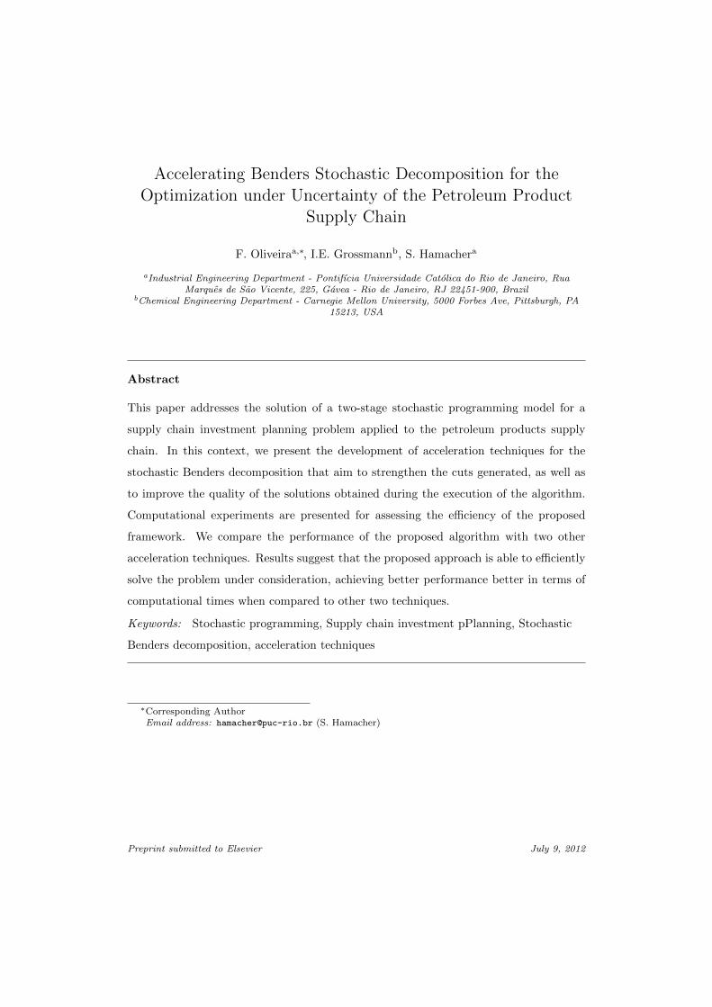
Figure 1: Example of a network

As shown in Figure 2, a supply chain is given composed of suppliers (represented by

source F1 and refinery R1) and demand points (represent by points B1 to B7), which are

connected through capacitated transportation arcs representing different transportation

modes (in this case, three modes are considered namely large ferries, small boats and

roadways). The demand points, which we will denote hereafter as distribution bases,

are allowed to store product if necessary, given that the problem is considered under a

multi-period setting. The storage and throughput capacities of the bases are limited,

although they can be improved through the implementation of expansion projects. The

same idea holds for arcs, which can also be expanded in the same fashion. In addition

to that, we also consider the possibility of building new arcs and bases.

The objective of the plan is to determine which of the possible investments should

be implemented and when, together with the transportation and inventory decisions

that will cope with the projected (although uncertain) growth of product demands while

minimizing both investment and logistics present costs.

To address the problem in question, a two-stage stochastic programming model is

proposed [3]. The first-stage comprises the decisions of which projects to implement and

when; the second-stage decisions are those relating to the flows of products, inventory

levels, supply provided to each demand site, and supply levels at sources. The purpose of

5

the model is to determine the optimal investment selection product distribution to meet

the demand of bases, minimizing both investment and logistics costs. The transporta-

tion decisions are defined in conjunction with investment decisions, which are chosen

from a predefined portfolio of possibilities and allocated over the planning horizon. The

uncertainties in the model are related to demand levels, which are modeled as random

variables.

The notation used to state the following model is given in Appendix A. The math-

ematical model for the optimization of the aforementioned problem can be stated as

follows:

minw,y∈0,1

∑j,p,t

Wjptwjpt +∑i,j,t

Yijtyijt +Q(w, y) (2.1)

s.t.:∑t

wjpt ≤ 1 ∀j ∈ B, p ∈ P (2.2)

∑t

yijt ≤ 1 ∀i, j ∈ N (2.3)

where wjpt represent the capacity expansion investment decisions at location j for product

p and in period t and yijt arc connecting locations i and j investment decisions in

period t, Q(w, y) = EΩ[Q(w, y, ξ)] represents the expectation evaluated over all ξ ∈ Ω

possible realizations for the uncertain parameters of the second-stage problem, given

an investment decision (w, y). Constraints 2.2 and 2.3 define that each investment can

happens only once along the time horizon considered.

The second-stage problem Q(w, y) can be stated as shown in equations 2.4 to 2.10.

The objective function 2.4 represents freight costs between nodes, inventory costs, and

cost of shortfall. Equation 2.5 comprises the material balance in distribution bases.

Constraint 2.6 limits the supply availability at sources. Constraint 2.7 defines the arc ca-

pacities and the possibility of its expansion through the investment decisions. In a similar

way, constraint 2.8 defines the storage capacities together with its expansion possibility.

Constraint 2.9 defines minimum inventory levels, according to safety requirements. Con-

straint 2.10 sets the throughput limit for bases, defined by the product of the available

6

storage capacity with the throughput capacity multiplier.

minx,v,u∈R+

∑ξ

P ξ

( ∑i,j,p,t

Cijtxξijpt +

∑j,p,t

Hjptvξjpt +

∑j,p,t

Sjptuξjpt

)(2.4)

s.t.:∑i

xξijpt + vξjpt−1 + uξjpt =∑i

xξjipt + vξjpt +Dξjpt ∀j ∈ B, p ∈ P, t ∈ T , ξ ∈ Ω (2.5)

∑j

xξijpt ≤ Oipt ∀i ∈ S, p ∈ P, t ∈ T , ξ ∈ Ω (2.6)

∑p

xξijpt ≤ A0ij +Aij

∑t′≤t

yijt′ ∀i, j ∈ N , t ∈ T , ξ ∈ Ω (2.7)

vξjpt ≤M0jp +Mjp

∑t′≤t

wjpt′ ∀j ∈ B, p ∈ P, t ∈ T , ξ ∈ Ω (2.8)

vξjpt ≥ Ljp

M0jp +Mjp

∑t′≤t

wjpt′

∀j ∈ B, p ∈ P, t ∈ T , ξ ∈ Ω (2.9)

∑i

xξijpt ≤ Kjp

M0jp +Mjp

∑t′≤t

wjpt′

∀j ∈ B, p ∈ P, t ∈ T , ξ ∈ Ω (2.10)

3. Stochastic Benders Decomposition

The model proposed in the previous section can be defined as an optimization model

with first-stage integer variables and second-stage continuous variables. Such character-

istics allow us to consider a scenario-wise decomposition framework based on Benders

decomposition [1] applied to stochastic optimization, given the particular diagonal struc-

ture of these problem, where the first-stage variables arise as complicating in a sense

that they are the only elements providing connection between each scenario subproblem

[29]. Moreover, the model has complete recourse [3], that is, for any feasible first-stage

solution, the second stage problem is always feasible. Note that this fact is convenient

since it precludes the generation of feasibility cuts in order to ensure feasibility in the

context of the stochastic Benders decomposition.

We start by noting that the MP can be equivalently reformulated as follows:

minw,y∈0,1

∑j,p,t

Wjptwjpt +∑i,j,t

Yijtyijt +M (3.1)

s.t.:7

∑t

wjpt ≤ 1 ∀j ∈ B, p ∈ P (3.2)

∑t

yijt ≤ 1 ∀i, j ∈ N (3.3)

M ≥ Q(w, y) (3.4)

This formulation allows one to distinguish an important issue. Inequality 3.4 cannot be

used computationally as a constraint since it is not defined explicitly, but only implicitly

by a number of optimization problems. The main idea of the proposed decomposition

method is to relax this constraint and replace it by a number of cuts, which may be

gradually added following an iterative solving process. These cuts, defined as supporting

hyperplanes of the second-stage objective function, might eventually provide a good

estimation for the value of Q(w, y) in a finite number of iterations. In order to define the

form of these cuts, let us first state the dual formulation of the second-stage problem,

which represents the SP in our context, given a first-stage solution (w, y):

Q(w, y) = EΩ[Q(w, y, ξ)] =

maxα,β,γ,δ,ζ,η

∑ξ

P ξ

(∑j,p,t

Dξjptα

ξjpt +

∑j,p,t

Ojptβξjpt+

∑i,j,t

A0ij +Aij

∑t′≤t

yijt′

γξijt+

∑j,p,t

M0jp +Mjp

∑t′≤t

wjpt

(δξjpt + Ljpη

ξjpt +Kjpζ

ξjpt

))(3.5)

s.t.:

αξjpt − αξipt + βξipt + γξjpt + ζξjpt ≤ Cijt ∀i, j ∈ N , p ∈ P, t ∈ T , ξ ∈ Ω (3.6)

αξjpt − αξjpt−1 + δξjpt + ηξjpt ≤ Hjpt ∀j ∈ B, p ∈ P, t ∈ T , ξ ∈ Ω (3.7)

αξjpt ≤ Sjpt ∀j ∈ S, p ∈ P, t ∈ T , ξ ∈ Ω (3.8)

Let Π denote the set of all extreme points of the polyhedron defined by the feasible space

of the Dual Slave Problem (DSP) given by 3.5 to 3.8 and α, β, γ, δ, ζ, and η denote the

dual variables associated with constraints 2.5 to 2.10, and M the objective function value.8

Also, letting M∗ be the optimal value, we must have M∗ ≥ M (k),∀k ∈ Π. Therefore,

our DSP can be restated as Q(w, y) = minM≥0M : M ≥M (k),∀k ∈ Π, where

M (k) =∑ξ∈Ω

P ξ

(∑j,p,t

Dξjptα

ξ(k)jpt +

∑j,p,t

Ojptβξ(k)jpt +

∑i,j,t

A0ij +Aij

∑t′≤t

yijt′

γξ(k)ijt +

∑j,p,t

M0jp +Mjp

∑t′≤t

wjpt

(δξ(k)jpt + Ljpη

ξ(k)jpt +Kjpζ

ξ(k)jpt

))(3.9)

Using the above representation for the DSP that is based on the extreme points k ∈ Π

of its polyhedron, we can now replace equation 3.4 with the new reformulation 3.9 for

EΩ[Q(w, y, ξ)] in the MP, providing the following:

minw,y∈0,1

∑j,p,t

Wjptwjpt +∑i,j,t

Yijtyijt +M (3.10)

s.t.:∑t

wjpt ≤ 1 ∀j ∈ B, p ∈ P (3.11)

∑t

yijt ≤ 1 ∀i, j ∈ N (3.12)

M ≥∑ξ∈Ω

P ξ

(∑j,p,t

Dξjptα

ξ(k)jpt +

∑j,p,t

Ojptβξ(k)jpt +

∑i,j,t

A0ij +Aij

∑t′≤t

yijt′

γξ(k)ijt +

∑j,p,t

M0jp +Mjp

∑t′≤t

wjpt

(δξ(k)jpt + Ljpη

ξ(k)jpt +Kjpζ

ξ(k)jpt

))∀k ∈ Π (3.13)

This reformulation has the drawback of comprising a very large number of constraints

of type 3.13. Moreover, at the optimal solution, not all of the constraints in 3.13 will be

binding. Therefore, in the iterative Benders decomposition algorithm, one works with a

relaxed version of MP by considering only a subset of 3.13 at each iteration. We denote

this subset by Π′ which includes the constraints 3.13 generated via solving the DSP in

the previous iterations. This relaxed formulation of the MP (RMP) considering only the

subset Π′ of cuts in 3.13 provides a lower bound to the optimal solution of the MP.9

At a given iteration of the stochastic Benders decomposition, a RMP(k) is solved first

to obtain the values of (w(k), y(k)). Then, these values are used to solve DSP(k) to obtain

the values of dual variables α(k), β(k), γ(k), δ(k), ζ(k), η(k) (i.e., an extreme point k ∈ Π

of the dual polyhedron) and a new cut of the form 3.13 to include into Π′. Note that

when the DSP(k) is solved for given (w(k), y(k)), an upper bound for MP can be easily

calculated by adding DSP(k)s objective value and the total fixed cost component for the

RMP(k) (i.e., the objective value of RMP(k) excluding M (k)).

4. Accelerating Benders Decomposition

In this section we present the techniques developed for speeding-up the decomposition

framework presented in the previous section.

4.1. Multi cut framework

Recall that in the stochastic Benders decomposition presented in the previous section,

a single optimality cut is added at each iteration. This cut aims to approximate the value

of the second-stage function at the current solution. However, instead of using only a

single cut at each iteration, one can add multiple cuts to approximate the individual

second-stage cost function corresponding to each one of the |Ω| scenarios. In this case,

the RMP can be reformulated as follows:

minw,y∈0,1

∑j,p,t

Wjptwjpt +∑i,j,t

Yijtyijt +Mξ (4.1)

s.t.:∑t

wjpt ≤ 1 ∀j ∈ B, p ∈ P (4.2)

∑t

yijt ≤ 1 ∀i, j ∈ N (4.3)

Mξ ≥∑j,p,t

Dξjptα

ξ(k)jpt +

∑j,p,t

Ojptβξ(k)jpt +

∑i,j,t

A0ij +Aij

∑t′≤t

yijt′

γξ(k)ijt +

∑j,p,t

M0jp +Mjp

∑t′≤t

wjpt

(δξ(k)jpt + Ljpη

ξ(k)jpt +Kjpζ

ξ(k)jpt

)∀ξ ∈ Ω, k ∈ Π′ (4.4)

10

Birge and Louveaux [2] showed that the use of such a framework may greatly speed-

up convergence. The main idea behind this multi cut framework is to generate an outer

linearization for all functions Q(w, y, ξ), replacing the outer linearization of Q(w, y). The

multi cut approach relies on the idea that using independent outer approximations of all

functions Q(w, y, ξ) provide more information to the MP than the single cut on Q(w, y),

and therefore, fewer iterations are needed to reach the optimal solution.

4.2. Generating stronger cuts

Magnanti and Wong [11] proposed a seminal methodology to accelerate convergence

of Benders decomposition by strengthening the generated cuts. They observed that in

certain cases where the SP presents degeneracy, one might generate different cuts for the

same optimal solution (w(k), y(k)), each one of different strength in terms of efficiently

approximating the second-stage cost function. To circumvent this difficulty, the authors

proposed a methodology for identifying the strongest possible cut, which they referred

to as the Pareto-optimal cut.

To illustrate the technique, assume that we have our problem written in the following

form:

mincT z + qT r|Az +Br ≥ h, z ∈ Z (4.5)

where Z ⊆ Rn represents linear constraints involving the first-stage n variables and their

integrality requirements, r ∈ Rp, A and B are m×n and m×p matrices, c ∈ Rn, q ∈ Rp,

and h ∈ Rm.

Similarly to what we did in Section 3, let Π = π ∈ Rm|BTπ ≤ q be the set of

feasible solutions for DSP. In addition, let M ≥ πT (h−Az) represent a Benders cut,

and Πalt be the set of alternative optimal solutions for the DSP given a MP solution

z. Then, we say that the Benders cut generated by π∗ dominates all others (i.e., is

Pareto-optimal) if:

π∗T (h−Az) ≤ πT (h−Az) ∀π ∈ Πalt (4.6)

Magnanti and Wong [11] showed how one can generates Pareto-optimal cuts based

on the notion of core points. A core point is defined as a point z in the relative interior

of Conv(Z), where Conv(·) denotes the convex hull [30]. They proved that if a cut is11

selected such that it attains the maximum value at a core point amongst the set of all

alternative cuts, then this cut is not dominated by other cuts at any feasible solution - a

Pareto-optimal cut.

In order to generate these cuts, they suggest selecting some core point z, and after

solving SP for z (which we denote hereafter as SP(z)), they generate the Benders cut by

subsequently solving a secondary subproblem, which can be stated as follows:

maxπT (h−Az) | π ∈ Πalt (4.7)

where Πalt = π ∈ Π | πT (h−Az) = f(SP (z)) is the set of alternative optimal solutions

of 4.7 and f(·) the objective function value.

Nevertheless, there are certain implementation issues related to Magnanti and Wong’s

cut generation procedure. First, the dependency of the subproblem 4.7 to the DSP might

jeopardize the algorithm efficiency, especially in the cases where the DSP might turn out

to be difficult to solve. Moreover, since Magnanti and Wong’s procedure requires a new

core point at each major iteration (recall that the core points rely inside the convex

hull of the MP, whose feasible region is changing at each major iteration), it might be

the case that it is not easy to obtain new core points at each iteration. To address this

drawback, researchers often approximate core points [24, 17], arbitrarily define it by fixing

components of the core point vector [13] or use alternative points derived from a given

problem structure [16]. In addition to that, it is important to note that this strategy does

not always yield a net computational advantage since the trade-off between the reduction

in the number of iterations required compared to the increase in the number of linear

programs solved to generate each cut might not pay-off [14].

In this paper we propose an alternative way of generating nondominated cuts based

on the definition of maximal cuts. Following the ideas of Sherali and Lunday [25] for gen-

erating maximal nondominated Benders cuts, we show an alternative for strengthening

the Benders Cuts while circumventing the aforementioned drawbacks.

First, we start by highlighting the standard definition of maximal, typically used in

cutting plane theory from integer programming literature [30]. Let us rewrite the Benders

cut generated from a selected π ∈ Πalt as:

M ≥ πTh+

n∑j=1

(−πTAj)zj (4.8)

12

Then, we say that a Benders cut is maximal for a given π if, for every π′ ∈ Πalt, we have

that πTh ≥ π′Th and −πTAj ≥ −π′TAj . It is not difficult to see that a Pareto-optimal

or nondominated cut generated in the way proposed by Magnanti and Wong [11] can be

also considered maximal, provided that the core point z is positive.

Sherali and Lunday [25] show that the aforementioned concept of maximal cuts can

be used to derive an alternative way of generating cuts that would accelerate Benders

decomposition. To achieve such a goal, we must first view the process of generating

maximal cuts as one of determining a Pareto-optimal solution to the multiple objective

problem defined as:

maxπTh,−πTA1, . . . ,−πTAn | π ∈ Πalt (4.9)

We can obtain a solution for this problem by selecting a positive weight vector (PWV)

and then maximizing the positive weighted sum of the multiple functions in 4.9 [27]. By

doing this, we end up by having to solve the following problem:

maxπTh+

n∑j=1

−πTAj z | π ∈ Πalt (4.10)

which is exactly the problem defined in 4.7. Therefore, if we define z as a positive core

point solution, then the resulting cut would be both maximal as well as nondominated.

Seeking to obtain an efficient framework to derive these cuts, we can combine in the

same problem both the step where we solve DSP(z) to obtain Πalt and the subsequent step

of solving 4.7. Toward this end, we must first note that we are essentially considering

a priority multiple objective program, where we want to first maximize DSP(z) (i.e.,

πT (h − Az) subject to π ∈ Π) and next, considering all alternative solutions to this

problem, choose the one which maximizes πT (h − Az). Again, one might note that the

approach of Magnanti and Wong [11] to generate nondominated cuts using the core point

z can be interpreted in the same way.

Sherali and Soyster [26] showed that such a multiple objective program can be equiv-

alently solved by the following combined weighted sum problem:

maxπT (h−Az) + µπT (h−Az) | π ∈ Π (4.11)

where µ is a suitably small weight. Although Sherali and Soyster [26] showed that it

is always possible to derive µ such that it would render 4.11 equivalent to the multi-13

objective problem mentioned before, the derivation of such a weight is not typically a

practically convenient task except in some particular cases.

In order to circumvent this drawback, we propose an alternative way of dealing with

the weight µ in order to obtain what we call as dynamically updated near-maximal Ben-

ders cuts. The main reasoning behind the following ideas are rather experimental than

theoretical. What we observe from our numerical experiments is that the solutions ob-

tained in the early iterations yield poor descriptions of the second-stage cost curve, which

is exactly what we are trying to approximate through the use of Benders cuts in the

stochastic programming context. Moreover, we observe that by applying the aforemen-

tioned ideas of generating maximal cuts, we can consider 4.11 as an auxiliary problem to

simulate the existence of more dense first-stage solutions in the early iterations in order

to speed-up the convergence. As for the algorithmic procedure, we can then iteratively

adjust the weight µ in order to favor solutions that are more focused on improving the

original DSP (z) objective value πT (h−Az) rather than 4.11.

One important characteristic of such a framework for updating the weight µ is that

it does not prevent convergence if a proper sequence µ(k)k=1,...,∞ is selected. In order

to keep the original convergence properties of the traditional Benders decomposition, it

follows that one might select a sequence of µb, b = 1, . . . ,∞ such that the following

properties hold:

1.∑∞k=1 µ

(k) →∞

2. µ(k) → 0 as k →∞

By selecting such a divergent series, its is not difficult to see that convergence is

guaranteed since:

limµ→0

πT (h−Az) + µπT (h−Az) = πT (h−Az) (4.12)

allowing us to rely on the results from Benders [1] (or from Van Slyke and Wets [29] for

the stochastic version, or even from Birge and Louveaux [2] for the multi cut framework),

which guarantees convergence for the algorithm.

4.3. Additional acceleration ideas

Combined with the strengthening of the cuts generated at each major iteration of

the proposed algorithm, we also use additional acceleration ideas in order to improve14

computational efficiency.

4.3.1. Upper bound improving

In our implementation of the stochastic Benders decomposition, we observed that

there is a strong relationship between the quality of the incumbent solutions (w, y) ob-

tained during the execution and the convergence rate of the algorithm. This issue is

related with the fact that, especially in the early iterations, the incumbent solutions

obtained may be quite far from the optimal solution, leading the algorithm to explore

inferior parts of the feasible region. However, if a good solution (w, y) is made available

through the use of some heuristic, we can use it in place of the incumbent solution and

proceed from there. Our algorithm makes use of a particular heuristic in order to try to

generate these good solutions during the algorithm execution.

The heuristic relies on facts observed during our computational experiments. We

observed that, after the optimality gap becomes reasonably small, the bounds exhibit

a tailing off behavior as the iterations progress. This effect is mainly due to the fact

that, in these iterations, all the incumbent solution tend to present identical or very

similar selection of projects (in terms of location and product for wjpt and origin and

destination for yijt), only changing timing decisions. Because the timing decisions have

relatively small influence on the objective value, the upper bound changes very little. In

order to avoid this behavior, this heuristic after a certain number of iterations with no

improvement on the upper bound. The heuristic consists of three main steps:

1. Fix the current project selection to those in the current incumbent solution.

2. Randomly sample a subset of the scenario set Ω and solve the equivalent deter-

ministic to determine whether this selection investment should be selected indeed,

and if so, when. Notice that by doing this, we are both reducing the size of the

second-stage problem (since it is a subset of Ω), as well as the size of the first-stage

problem (since we are only considering investments decided in terms of location

and product for wjpt and origin and destination for yijt, hence considering fewer

integer variables).

3. Evaluate the obtained solution to check if it provides an improved upper bound. If

so, use this solution to update the incumbent solution and the correspondent upper

bound as the incumbent upper bound.15

4.3.2. Trust-region

As pointed out by Ruszczynski [20], the initial iterations of decomposition methods

based on cutting planes tend to present an unstable behavior. This effect is mainly due

to the fact that the solutions tend to oscillate between different sections of the feasible

region, what may lead to slow convergence.

In the continuous case, this effect can be effectively controlled by the use of two

different approaches. The first consists of adding a regularizing term in the MP objective

function that penalizes the l2-distance between the current solution and the previous one

[20]. The second focuses on constraining the l∞ distance of the MP variables from the

previous solution within a trust region [9]. These extensions prevent the MP solution

from moving far from the previous iterate. One point that must be highlighted is that

both the penalty magnitude and the size of the trust region must be controlled during

the execution of the algorithm based on its progress. Using a proper control is imperative

when using these techniques in order to avoid losing convergence properties.

In our problem, the first-stage variables are binary vectors. In this case, using a

l2 regularizing term would render a mixed-integer quadratic MP, which would become

much more complex in terms of solution methodology. Moreover, a l∞ trust-region

would be useless in our case. Since feasible MP solutions are extreme points of the unit

hypercube, a trust region of size greater or equal than one would include all its vertices

(i.e., all possible binary feasible solutions), while a trust-region with size less than one

would include only the previous solution.

Santoso et al. [24] show how one can deal with this drawback by using the Hamming

distances between the binary solution vector as a measuring unit for the trust region.

Let (w(k), y(k)) be the MP in iteration k and let W = (j, p, t) | w(k)jpt = 1 and Y =

(i, j, t) | y(k)ijt = 1. Then, we impose the following constraint in the MP to be solved in

iteration k + 1:∑(j,p,t)∈W

(1− wjpt) +∑

(i,j,t)∈Y

(1− yijt)+

∑(j,p,t)/∈W

wjpt +∑

(i,j,t)/∈Y

yijt ≤ Γ(k+1) (4.13)

where Γ(k+1) < (|N × P × T |+ |N ×N × T |) represents the trust-region size in itera-

16

tion k + 1. Unfortunately, convergence cannot be guaranteed if a non-redundant trust

region is used throughout the algorithm execution. Hence, since the algorithm tends to

have the oscillating effect that we are willing to avoid mostly in the beginning of the ex-

ecution, we dynamically adjust the size as the algorithm converges. When the algorithm

reaches a sufficiently small optimality gap, we drop 4.13 from the MP in order to ensure

convergence.

5. Computational Experiments

This section describes the computational experiments performed to evaluate the pro-

posed algorithm under different considerations. All experiments described in this sec-

tion were executed in an Intel Xeon 2.4GHz CPU with 4GB RAM and implemented in

AIMMS 3.12. The mixed-integer and linear programming models within the decomposi-

tion framework were solved with CPLEX 12.3.

In order to assess the efficiency of the proposed framework, we consider two different

instances. The first consists of a small example formulated to illustrate the efficiency of

the proposed approach. The second example consists of a realistic case study of a large-

scale investment planning problem. We test both instances comparing the results with

three different techniques. The first technique used (for now on referred as Algorithm

1 ) generates nondominated Benders cuts according to Magnanti and Wong [11], with

the approximation and core point updating technique as proposed by Papadakos [16],

i.e., we initialize a core point approximation z with a feasible solution to the MP and

then update the approximation at each successive iteration by setting z = λz+ (1−λ)z.

We adopt λ = 0.5, as prescribed by Papadakos [16]. The author states that, based

on empirical observation, such a value for λ usually yields better results in terms of

algorithmic convergence. The second technique (Algorithm 2 ) used consists of generating

maximal nondominated Benders cut as proposed by Sherali and Lunday [25]. The authors

show that one can use the following expression to calculate µ that yields a near-optimal

maximal Benders cut:

µ =ε0Mθ

(5.1)

where ε is a prespecified tolerance on the absolute optimality gap, M is the penalty for

17

recourse unfeasibility (that is equivalent to the cost of unmet demand in our case), and

θ = ε0 + max0,maxhi −min0,minhi, with h = h− Az. We used a fixed value

for the weight µ, as shown by the authors in their calculations, considering ε0 as being

1% of the true optimal value for Example 1. In Example 2, we empirically derived a

fixed value for µ, since it is not practically convenient to base the selection of ε0 on

the optimal solution. Note that by doing that, we are in effect implicitly dictating a

particular choice of ε0. Finally, Algorithm 3 use the dynamically updated near maximal

Benders cuts proposed in section 4.2 as the cut generation strategy. In both cases we

update the multipliers according to the following divergent series:

µt+1 =k

l|B|µt (5.2)

where k and l are pre specified parameters, and |B′| represents the number of iterations

up to now. In both experiments we use k = 2, l = 1, and µ0 is given by 5.1. We use ε0 as

5% of the true optimal value for Example 1 and an empirically fixed value for Example

2.

5.1. Example 1

The first example is a simplified version of the investment planning model introduced

in Section 2. It involves capacity expansions and network design decisions for a simplified

network composed by three supply sites, five primary bases (intermediate markets which

works also as distribution points), and four secondary bases (which are equivalent to

final markets) as seen in Figure 2. We consider five time periods and sixteen scenarios

for the demand at both primary and secondary bases. For generating the scenarios we

consider that the demand in each region can either grow 5% per year, or decrease 1%

per year. We consider that the example comprises five different regions: B1 and B2 as

Region 1, B3 as Region 2, B4 and B5 as Region 3, C1 and C2 as Region 4, and C3 and

C4 as Region 5. The data considered for this experiment is given in Appendix B.

The equivalent deterministic model has 80 binary variables, 2803 continuous vari-

ables, and 3859 constraints. The optimal solution of this problem is $1,520.47 million

over a five-year period. The optimal first-stage solution is illustrated in Figure 2. The

arcs between two different regions (represented by gray background rectangles) are the

arcs that can be selected to compose the network design, while the second row of nodes18

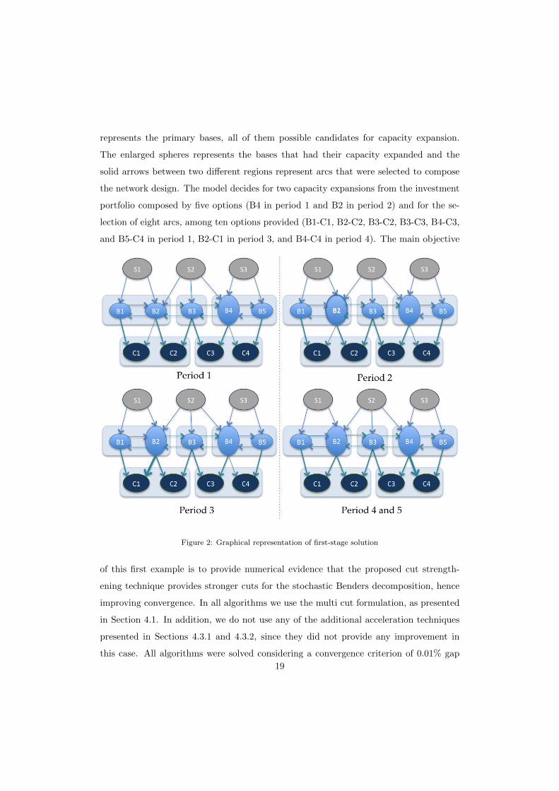
represents the primary bases, all of them possible candidates for capacity expansion.

The enlarged spheres represents the bases that had their capacity expanded and the

solid arrows between two different regions represent arcs that were selected to compose

the network design. The model decides for two capacity expansions from the investment

portfolio composed by five options (B4 in period 1 and B2 in period 2) and for the se-

lection of eight arcs, among ten options provided (B1-C1, B2-C2, B3-C2, B3-C3, B4-C3,

and B5-C4 in period 1, B2-C1 in period 3, and B4-C4 in period 4). The main objective

Figure 2: Graphical representation of first-stage solution

of this first example is to provide numerical evidence that the proposed cut strength-

ening technique provides stronger cuts for the stochastic Benders decomposition, hence

improving convergence. In all algorithms we use the multi cut formulation, as presented

in Section 4.1. In addition, we do not use any of the additional acceleration techniques

presented in Sections 4.3.1 and 4.3.2, since they did not provide any improvement in

this case. All algorithms were solved considering a convergence criterion of 0.01% gap

19

between upper and lower bounds.

Table 1 summarizes the performance of each cut generation technique, compared with

the use of traditional Benders cuts. The computational results allow us to draw two im-

portant observations. First, one can notice that all acceleration techniques improved the

algorithm efficiency in terms of number of iterations to reach the convergence criterion,

and consequently, in terms of computational time, when compared with the traditional

Benders cut generation procedure. Second, one can observe that, even though the three

algorithms provide similar results, the proposed approach (Algorithm 3 ) is be able to

reach the optimal solution slightly faster.

Traditional Cuts Algorithm 1 Algorithm 2 Algorithm 3

# of iterations 35 21 26 19

CPU Time[s] 10.93 5.90 7.22 4.86

Table 1: Example 1 result summary

5.2. Example 2

The second example represents a realistic supply chain investment planning problem

under demand uncertainty. The transportation can in principle be performed in different

modes, but in this case study it is primarily done using waterways, which are strongly

affected by seasonality issues regarding the navigability of rivers. Four different products

were considered - diesel, gasoline, aviation fuel and fuel oil - to be distributed over

19 locations (13 bases and 1 refinery and 2 external supply locations). The portfolio of

projects considered for the study consists of 28 local projects and three arc projects. The

planning horizon considered was 6 years, divided into a total of 24 quarterly periods. All

experiments in this example were solved up to 2% optimality gap. For further details on

this instance, please refer to Oliveira and Hamacher [15].

To take into account the uncertainty in demand levels for petroleum products, sce-

narios were generated by the following first order autoregressive model:

Djpt = Djpt−1 (1 + ωp + σε) (5.3)

where ωp represents the expected average growth rate for the consumption of product p

over the planning horizon, σ represents the estimated maximum deviation for product20

consumption in the region and ε follows a standard normal distribution. The average

growth rate, as well as the maximum deviation were forecasted based on the analysis of

the annual consumption historical series over the last 40 years. Each scenario represents

a possible demand curve for the whole time horizon considered, for each product and

place.

In order to assess the efficiency of the proposed approach, we performed two different

experiments. The first experiments seeks to illustrate the effects of using the accelera-

tion techniques proposed in sections 4.3.1 (Upper bounding improving) and 4.3.2(Trust

regions) in a random sample composed by 200 scenarios. Table 2 summarizes the perfor-

mance of these techniques compared them individually and in combination with the case

where none of such acceleration techniques are used. Note that in Table 2 the bounds

are not reported at their last iteration since we are using arbitrary increments in the

number of iterations.

# Iter.No Acc. UB Imp. TR UB Imp. + TR

UB %gap UB %gap UB %gap UB %gap

1 1732310.5 99.2 1732310.5 99.2 1732310.5 99.2 1732310.5 99.2

5 481802.2 46.3 481802.2 46.4 481802.2 46.4 481802.2 46.3

10 418213.5 7.3 416152.5 10.1 416152.5 3.4 418213.5 7.3

15 412056.4 3.7 408188.4 2.5 411950.4 2.5 408188.4 2.4

20 412056.4 2.7 - - 411950.4 - - -

25 412056.4 2.3 - - - - - -

30 412056.4 2.1 - - - - - -

CPU Time[s] 1151.2 617.7 619.0 446.3

Table 2: Example 2 result summary - experiment 1

Table 2 allows us to observe the effect of the acceleration techniques proposed in

Sections 4.3.1 and 4.3.2 separately (indicated as UB Imp. and TR, respectively). From

the results we can conclude that both techniques improve convergence of the proposed

algorithm, reducing the total CPU time required to reach the convergence criterion by

approximately 46% in both cases. Moreover, when we combine both techniques, the

reduction in the solution times is even larger, yielding improvement on the solution time

21

of over 61%.

For the second experiment in this example, we developed a set consisting of 100

independent scenario samples of sizes varying from 20 to 200 scenarios, as can be seem in

Table 3. Notice that in this case, we are solving the problem for 1000 different demand

instances, since the samples are independent. Our objective by doing that is to assess

the efficiency of the proposed approach independent of particularities of a given scenario

sample.

ScenariosAlgorithm 1 Algorithm 2 Algorithm 3 CPLEX

Avg. St. Dev. Avg. St. Dev. Avg. St. Dev. Avg. St. Dev.

20 56.5 19.2 55.5 15.0 22.3 2.2 9.6 0.6

40 104.7 37.7 102.1 31.3 43.2 2.7 33.7 3.3

60 162.4 66.5 140.7 52.0 64.0 4.5 51.5 5.0

80 219.5 78.6 221.5 111.8 83.7 5.8 104.0 20.9

100 287.2 124.3 272.5 139.2 109.1 12.7 185.6 34.5

120 369.6 150.5 313.9 152.4 128.3 9.2 287.8 46.3

140 387.6 163.3 381.8 170.9 151.2 10.8 473.0 122.3

160 483.8 208.8 372.3 135.8 176.7 11.6 601.1 140.8

180 612.7 270.3 477.1 189.4 203.8 13.9 734.9 165.6

200 631.4 252.7 521.8 196.1 230.1 12.2 927.6 161.0

Table 3: Example 2 result summary of CPU-times - experiment 2

Table 3 presents the statistical data retrieved from the experiments carried out in

Example 2, showing the average time solution (Avg. column) and the standard deviation

(Std. Dev. column) in CPU seconds. As can be seen in Table 3, the CPLEX times are

smaller in the experiments when a small number of scenarios is considered. However,

it is important to keep in mind that these examples with smaller number of scenarios

are only for completeness of the experimental set since they are not capable of giving a

good description of the uncertainty considered (for further information on sample size

specifications, please refer to Oliveira and Hamacher [15]). As the number of scenarios

increases, the decomposition frameworks outperform the use of CPLEX. We also highlight

the performance of our algorithm (Algorithm 3 ) in the case study under consideration.

22

As we can be observe from the experimental results, the proposed algorithm performed

better than the other cutting generation strategy in all experiments. In addition, for

cases where more than 80 scenarios where considered, Algorithm 3 reached the best

average solution times among all solution procedures, including CPLEX.

Another remarkable feature that can be observed in Table 3 is related to the standard

deviation of the solution times. The results suggest that Algorithm 3 attains the smaller

deviation in terms of CPU seconds regarding the time the algorithm takes to reach a 2%

gap suboptimal solution. The observation of this fact lead us to the conclusion that the

performance of our textitAlgorithm 3 is less affected by particular characteristics of the

scenario sample itself since it seems to be more robust in terms of solution time variation.

6. Conclusions

In this paper we have presented the development of acceleration techniques for the

stochastic Benders decomposition to solve an investment planning problem applied to the

petroleum products supply chain. We have proposed a new methodology for generat-

ing dynamically updated near-maximal Benders cuts, and compared it with acceleration

techniques proposed by Papadakos [16] and Sherali and Lunday [25] for the stochastic

Benders algorithm. Moreover, we have proposed the application of two additional ac-

celeration techniques to further improve the convergence of the algorithm, especially in

cases where convergence is difficult due to the computational complexity of the problem

at hand.

We conducted two numerical examples to assess the efficiency of the proposed frame-

work. In Example 1 we showed how the acceleration technique can be applied to a small

problem. The results provide some numerical evidences regarding the benefits one could

obtain by using the proposed acceleration technique. In Example 2 we tackled a large-

scale real world problem. Since we are dealing with uncertainty through the use of a

sampling framework, we choose to generate a large number of instances (100 samples of

10 different sizes) by repeatedly sampling a first order autoregressive model. The problem

considered represents a realistic supply chain investment planning problem considering

four different products to be distributed over 19 locations (13 bases, 1 refinery and 2 ex-

ternal supply locations). As our computational results suggest, our algorithm performed

23

faster for this particular problem considered under a sampling framework. The experi-

mental results show that, for a larger number of scenarios, the proposed algorithm can

perform 4.5 times faster on average than solving the full-space equivalent deterministic

problem. Moreover, our algorithm also presented better results when compared to other

acceleration approaches considered.

As for future research, we are seeking to further evaluate the technique under a more

broader context, testing these ideas for more general types of problems commonly used

in the literature. We also believe that the development of more exhaustive sensitivity

analysis of the algorithmic performance to variations in user-specified parameters deserve

further examination in a future study.

7. References

[1] Benders, J., 1962. Partitioning procedures for solving mixed-variables programming problems. Nu-

merische mathematik 4 (1), 238–252.

[2] Birge, J., Louveaux, F., 1988. A multicut algorithm for two-stage stochastic linear programs. Eu-

ropean Journal of Operational Research 34 (3), 384–392.

[3] Birge, J., Louveaux, F., 1997. Introduction to stochastic programming. Springer Verlag.

[4] Cordeau, J., Soumis, F., Desrosiers, J., 2000. A benders decomposition approach for the locomotive

and car assignment problem. Transportation Science 34 (2), 133–149.

[5] Cote, G., Laughton, M., 1984. Large-scale mixed integer programming: Benders-type heuristics.

European Journal of Operational Research 16 (3), 327–333.

[6] Fischetti, M., Salvagnin, D., Zanette, A., 2010. A note on the selection of benders cuts. Mathemat-

ical Programming 124 (1), 175–182.

[7] Franca, P., Luna, H., 1982. Solving stochastic transportation-location problems by generalized

benders decomposition. Transportation Science 16 (2), 113–126.

[8] Geoffrion, A., Graves, G., 1974. Multicommodity distribution system design by benders decompo-

sition. Management science, 822–844.

[9] Linderoth, J., Wright, S., 2003. Decomposition algorithms for stochastic programming on a com-

putational grid. Computational Optimization and Applications 24 (2), 207–250.

[10] Magnanti, T., Mireault, P., Wong, R., 1986. Tailoring benders decomposition for uncapacitated

network design. Netflow at Pisa, 112–154.

[11] Magnanti, T., Wong, R., 1981. Accelerating benders decomposition: Algorithmic enhancement and

model selection criteria. Operations Research, 464–484.

[12] McDaniel, D., Devine, M., 1977. A modified benders’ partitioning algorithm for mixed integer

programming. Management Science, 312–319.

24

[13] Mercier, A., Cordeau, J., Soumis, F., 2005. A computational study of benders decomposition for

the integrated aircraft routing and crew scheduling problem. Computers & Operations Research

32 (6), 1451–1476.

[14] Mercier, A., Soumis, F., 2007. An integrated aircraft routing, crew scheduling and flight retiming

model. Computers & Operations Research 34 (8), 2251–2265.

[15] Oliveira, F., Hamacher, S., 2012. Optimization of the petroleum product supply chain under un-

certainty: A case study in northern brazil. Industrial & Engineering Chemistry Research 51 (11),

4279–4287.

[16] Papadakos, N., 2008. Practical enhancements to the magnanti-wong method. Operations Research

Letters 36 (4), 444–449.

[17] Papadakos, N., 2009. Integrated airline scheduling. Computers & Operations Research 36 (1), 176–

195.

[18] Peng, X., Jirutitijaroen, P., 2010. Convergence acceleration techniques for the stochastic unit com-

mitment problem. In: Probabilistic Methods Applied to Power Systems (PMAPS), 2010 IEEE 11th

International Conference on. IEEE, pp. 364–371.

[19] Rei, W., Gendreau, M., Soriano, P., Centre interuniversitaire de recherche sur les reseaux

d’entreprise, l. l. e. l. t., 2007. Local branching cuts for the 0-1 integer L-Shaped algorithm. CIR-

RELT.

[20] Ruszczynski, A., 1997. Decomposition methods in stochastic programming. Mathematical program-

ming 79 (1), 333–353.

[21] Saharidis, G., Boile, M., Theofanis, S., 2011. Initialization of the benders master problem using valid

inequalities applied to fixed-charge network problems. Expert Systems with Applications 38 (6),

6627–6636.

[22] Saharidis, G., Ierapetritou, M., 2010. Improving benders decomposition using maximum feasible

subsystem (mfs) cut generation strategy. Computers & chemical engineering 34 (8), 1237–1245.

[23] Saharidis, G., Minoux, M., Ierapetritou, M., 2010. Accelerating benders method using covering cut

bundle generation. International Transactions in Operational Research 17 (2), 221–237.

[24] Santoso, T., Ahmed, S., Goetschalckx, M., Shapiro, A., 2005. A stochastic programming approach

for supply chain network design under uncertainty. European Journal of Operational Research

167 (1), 96–115.

[25] Sherali, H., Lunday, B., 2011. On generating maximal nondominated benders cuts. Annals of Op-

erations Research, 1–16.

[26] Sherali, H., Soyster, A., 1983. Preemptive and nonpreemptive multi-objective programming: Rela-

tionship and counterexamples. Journal of Optimization Theory and Applications 39 (2), 173–186.

[27] Steuer, R., 1989. Multiple criteria optimization: Theory, computation, and application. Krieger

Malabar, FL.

[28] Uster, H., Agrahari, H., 2011. A benders decomposition approach for a distribution network design

problem with consolidation and capacity considerations. Operations Research Letters.

[29] Van Slyke, R., Wets, R., 1969. L-shaped linear programs with applications to optimal control and

25

stochastic programming. SIAM Journal on Applied Mathematics, 638–663.

[30] Wolsey, L., 1998. Integer programming.

[31] Yang, Y., Lee, J., 2011. Acceleration of benders decomposition for mixed integer linear program-

ming. In: Advanced Control of Industrial Processes (ADCONIP), 2011 International Symposium

on. IEEE, pp. 222–227.

26

Appendix A. Nomenclature

Indexes and sets

i, j ∈ N Locations

p ∈ P Products

t ∈ T Time periods

ξ ∈ Ω Scenarios

Subsets

B ⊆ N Distribution bases

S ⊆ N Suppliers

Parameters

A0ij Current arc capacity

Aij Additional arc capacity

Cijt Transportation cost

Dξjpt Demand

Hjpt Inventory cost

Kjp Throughput capacity multiplier

M0jp Current inventory capacity

Mjp Additional inventory capacity

Ojpt Supply

Sjpt Shortfall cost

Wjpt Inventory investment cost

Yijt Arc investment cost

Variables

xξijpt Product flow

vξjpt Inventory level

uξjpt Unmet demand

wjpt Inventory investment decision

yijt Arc investment decision

Table A.4: Model Notation

27

Appendix B. Data of the Experiment 1

Arc Freight Cost [$/m3] Investment Cost[1000$]

B1 C1 0.1 11

B2 B1 0 20

B2 B3 1.2 15

B2 C1 0 17

B2 C2 0 13

B3 B2 1.6 13

B3 B4 1.8 19

B3 C2 0 16

B3 C3 0 16

B4 B3 1.1 15

B4 B5 0.2 -

B4 C3 0 13

B4 C4 0 12

B5 B4 0.3 -

B5 C4 0 10

Table B.5: Example 1 data: Arc freight and investment cost

28

BaseInitial Capacity Expansion Capacity Investment Cost Inventory Cost

[1000m3] [1000m3] [1000$] [$/m3]

B1 40 8 752 0.5

B2 30 6 528 0.7

B3 40 8 712 1

B4 30 12 996 0.2

B5 50 10 800 1

Table B.6: Example 1 data: locations initial capacity, expansion capacity, investment cost, and inventory

cost

Supply Limit [m3] 100

Arc Capacity [1000m3] 50

Throughput Capacity Adjustment Factor 1.5

Return Rate 8%

Safety Level 10%

Table B.7: Example 1 data: general parameters

Base Initial Demand [1000m3]

B1 30

B2 25

B3 30

B4 40

B5 30

C1 10

C2 15

C3 20

C4 15

Table B.8: Example 1 data: base initial demands

29