Benders Decomposition for Solving Two-stage Stochastic ... · Benders Decomposition for Solving Two-stage Stochastic Optimization Models IMA New Directions Short Course on Mathematical

Benders Decomposition for Solving Two-stageStochastic Optimization Models

IMA New Directions Short Course on Mathematical Optimization

Jim Luedtke

Department of Industrial and Systems EngineeringUniversity of Wisconsin-Madison

August 9, 2016

Jim Luedtke (UW-Madison) Benders Decomposition Lecture Notes 1 / 33

Basic Benders

Review – Two-Stage Stochastic LP with Recourse

zSP = min c>x+∑S

s=1 psQs(x)

s.t. Ax ≥ bx ∈ Rn1

+

where for s = 1, . . . , S

Qs(x)def= Q(x, ξs) = min q>s y

s.t. Wsy = hs − Tsxy ∈ Rn2

+

How to solve this problem?

Yesterday: Deterministic equivalent form ⇒ Large-scale LP

Today: Benders decomposition ⇒ Exploit structure


Basic Benders

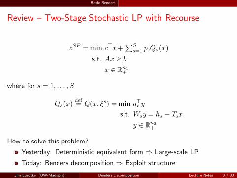
Common Assumption

Relatively Complete Recourse

For every feasible first-stage feasible solution (Ax ≥ b, x ∈ Rn1+ ) and

every scenario s there exists a feasible recourse decision ys (Wsys =hs − Tsx, ys ∈ Rn2

+ ).

Simplifies Benders decomposition algorithm

We’ll first present the algorithm under this assumption

Then relax the assumption

Assumption is very important when using sample average approximation

Relatively complete recourse should hold for all possible realizations ofrandom outcomes

Otherwise, solution to SAA problem may not even be feasible tooriginal problem


Basic Benders

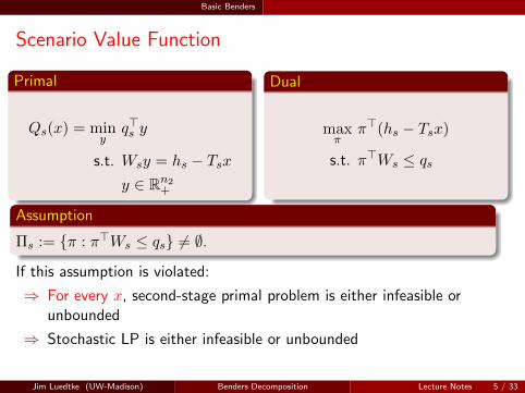
Scenario Value Function

Primal

Qs(x) = miny

q>s y


+

Dual

maxπ

π>(hs − Tsx)

s.t. π>Ws ≤ qs

Assumption

Πs := π : π>Ws ≤ qs 6= ∅.

If this assumption is violated:

⇒ For every x, second-stage primal problem is either infeasible orunbounded

⇒ Stochastic LP is either infeasible or unbounded


Basic Benders

Scenario Value Function

Primal

Qs(x) = miny

q>s y


+

Dual

maxπ

π>(hs − Tsx)

s.t. π>Ws ≤ qs

Assumption

Πs := π : π>Ws ≤ qs 6= ∅.

Relatively complete recourse ⇒ Primal has a feasible solution

Strong duality applies: Primal and dual each have an optimal solution


Basic Benders

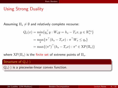
Using Strong Duality

Assuming Πs 6= ∅ and relatively complete recourse:

Qs(x) = minyq>s y : Wsy = hs − Tsx, y ∈ Rn2

+

= maxππ>(hs − Tsx) : π>Ws ≤ qs

= max(πs)>(hs − Tsx) : πs ∈ XP(Πs)

where XP(Πs) is the finite set of extreme points of Πs.

Structure of Qs(·)Qs(·) is a piecewise-linear convex function.


Basic Benders

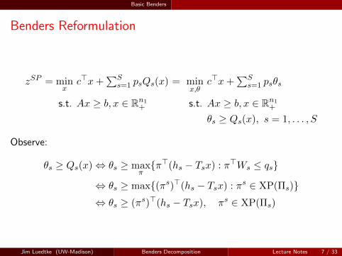
Benders Reformulation

zSP = minx

c>x+∑S

s=1 psQs(x) = minx,θ

c>x+∑S

s=1 psθs

s.t. Ax ≥ b, x ∈ Rn1+ s.t. Ax ≥ b, x ∈ Rn1

+

θs ≥ Qs(x), s = 1, . . . , S

Observe:

θs ≥ Qs(x)⇔ θs ≥ maxππ>(hs − Tsx) : π>Ws ≤ qs

⇔ θs ≥ max(πs)>(hs − Tsx) : πs ∈ XP(Πs)⇔ θs ≥ (πs)>(hs − Tsx), πs ∈ XP(Πs)


Basic Benders

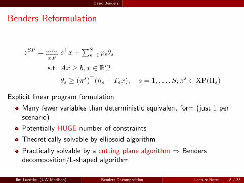
Benders Reformulation

zSP = minx,θ

c>x+∑S

s=1 psθs

s.t. Ax ≥ b, x ∈ Rn1+

θs ≥ (πs)>(hs − Tsx), s = 1, . . . , S, πs ∈ XP(Πs)

Explicit linear program formulation

Many fewer variables than deterministic equivalent form (just 1 perscenario)

Potentially HUGE number of constraints

Theoretically solvable by ellipsoid algorithm

Practically solvable by a cutting plane algorithm ⇒ Bendersdecomposition/L-shaped algorithm


Basic Benders

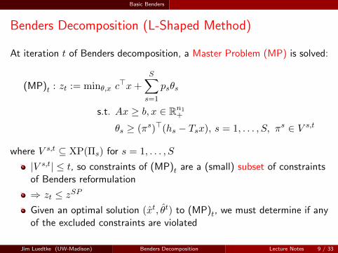
Benders Decomposition (L-Shaped Method)

At iteration t of Benders decomposition, a Master Problem (MP) is solved:

(MP)t : zt := minθ,x c>x+

S∑s=1

psθs

s.t. Ax ≥ b, x ∈ Rn1+

θs ≥ (πs)>(hs − Tsx), s = 1, . . . , S, πs ∈ V s,t

where V s,t ⊆ XP(Πs) for s = 1, . . . , S

|V s,t| ≤ t, so constraints of (MP)t are a (small) subset of constraintsof Benders reformulation

⇒ zt ≤ zSP

Given an optimal solution (xt, θt) to (MP)t, we must determine if anyof the excluded constraints are violated


Basic Benders

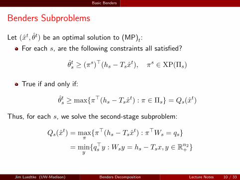
Benders Subproblems

Let (xt, θt) be an optimal solution to (MP)t:

For each s, are the following constraints all satisfied?

θts ≥ (πs)>(hs − Tsxt), πs ∈ XP(Πs)

True if and only if:

θts ≥ maxπ>(hs − Tsxt) : π ∈ Πs = Qs(xt)

Thus, for each s, we solve the second-stage subproblem:

Qs(xt) = max

ππ>(hs − Tsxt) : π>Ws = qs

= minyq>s y : Wsy = hs − Tsx, y ∈ Rn2

+


Basic Benders

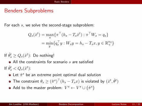
Benders Subproblems

For each s, we solve the second-stage subproblem:

Qs(xt) = max

ππ>(hs − Tsxt) : π>Ws = qs

= minyq>s y : Wsy = hs − Tsx, y ∈ Rn2

+

If θts ≥ Qs(xt): Do nothing!

All the constraints for scenario s are satisfied

If θts < Qs(xt):

Let πs be an extreme point optimal dual solution

The constraint θs ≥ (πs)>(hs − Tsx) is violated by (xt, θt)

Add to the master problem: V s ← V s ∪ πs


Basic Benders

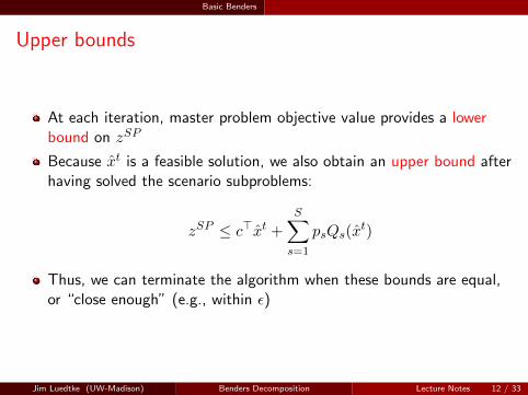
Upper bounds

At each iteration, master problem objective value provides a lowerbound on zSP

Because xt is a feasible solution, we also obtain an upper bound afterhaving solved the scenario subproblems:

zSP ≤ c>xt +

S∑s=1

psQs(xt)

Thus, we can terminate the algorithm when these bounds are equal,or “close enough” (e.g., within ε)


Basic Benders

Recap: Benders Decomposition

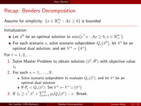
Assume for simplicity: x ∈ Rn1+ : Ax ≥ b is bounded

Initialization:

Let x0 be an optimal solution to minc>x : Ax ≥ b, x ∈ Rn1+

For each scenario s, solve scenario subproblem Qs(x0), let πs be an

optimal dual solution, and set V s = πs.For t = 1, 2, . . .

1. Solve Master Problem to obtain solution (xt, θt) with objective valuezt

2. For each s = 1, . . . , S:

Solve scenario subproblem to evaluate Qs(xt), and let πs be an

optimal dual solutionIf θts < Qs(x

t): Set V s ← V s ∪ πs3. If zt ≥ c>xt +

∑Ss=1 psQs(x

t)− ε: Break.


Basic Benders

Convergence

The algorithm trivially terminates finitely

Only finitely many extreme point dual solutions

If no new cuts added, lower and upper bounds will be equal

But no guarantee on rate of convgerence (similar to simplex)

In practice, often converges “pretty fast”, but occasionally disastrous


Basic Benders

Implementation Notes

Must use a cut violation tolerance, e.g., δ ≈ 10e−6:

Numerically, conclude θts < Qs(xt) only if θts < Qs(x

t)− δδ should match the feasibility tolerance of LP solver

Otherwise, you may add a “cut” that LP solver does not think isviolated ⇒ infinite loop

Not necessary to solve all scenario subproblems in every iteration

But only obtain an upper bound (and hence can consider terminating)when all are solved

Focus on “useful” scenarios

Scenario subproblems can be solved in parallel

Parallel scalability eventually limited by master problem


Basic Benders Example

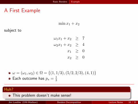
A First Example

minx1 + x2

subject to

ω1x1 + x2 ≥ 7

ω2x1 + x2 ≥ 4

x1 ≥ 0

x2 ≥ 0

ω = (ω1, ω2) ∈ Ω = (1, 1/3), (5/2, 2/3), (4, 1)Each outcome has ps = 1

3

Huh?

This problem doesn’t make sense!


Basic Benders Example

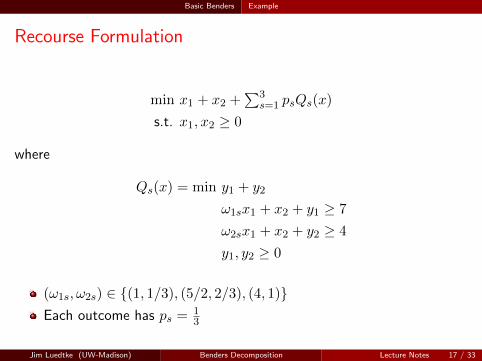
Recourse Formulation

min x1 + x2 +∑3

s=1 psQs(x)

s.t. x1, x2 ≥ 0

where

Qs(x) = min y1 + y2

ω1sx1 + x2 + y1 ≥ 7

ω2sx1 + x2 + y2 ≥ 4

y1, y2 ≥ 0

(ω1s, ω2s) ∈ (1, 1/3), (5/2, 2/3), (4, 1)Each outcome has ps = 1

3


Handling Infeasible Subproblems

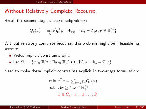
Without Relatively Complete Recourse

Recall the second-stage scenario subproblem:


+

Without relatively complete recourse, this problem might be infeasible forsome x:

Yields implicit constraints on x

Let Cs = x ∈ Rn1 : ∃y ∈ Rn2+ s.t. Wsy = hs − Tsx

Need to make these implicit constraints explicit in two-stage formulation:

min c>x+∑S

s=1 psQs(x)

s.t. Ax ≥ b, x ∈ Rn1+

x ∈ Cs, s = 1, . . . , S



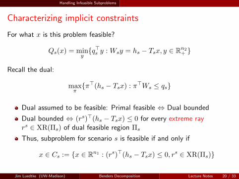
Characterizing implicit constraints

For what x is this problem feasible?


+

Recall the dual:

maxππ>(hs − Tsx) : π>Ws ≤ qs

Dual assumed to be feasible: Primal feasible ⇔ Dual bounded

Dual bounded ⇔ (rs)>(hs − Tsx) ≤ 0 for every extreme rayrs ∈ XR(Πs) of dual feasible region Πs

Thus, subproblem for scenario s is feasible if and only if

x ∈ Cs := x ∈ Rn1 : (rs)>(hs − Tsx) ≤ 0, rs ∈ XR(Πs)



Modified Benders Reformulation

minx,θ

c>x+∑S

s=1 psθs

s.t. Ax ≥ b, x ∈ Rn1+

θs ≥ (πs)>(hs − Tsx), s = 1, . . . , S, πs ∈ XP(Πs)

(rs)>(hs − Tsx) ≤ 0, s = 1, . . . , S, rs ∈ XR(Πs)

Again can solve with a cutting plane algorithm



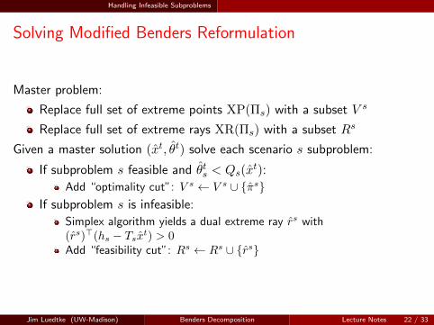
Solving Modified Benders Reformulation

Master problem:

Replace full set of extreme points XP(Πs) with a subset V s

Replace full set of extreme rays XR(Πs) with a subset Rs

Given a master solution (xt, θt) solve each scenario s subproblem:

If subproblem s feasible and θts < Qs(xt):

Add “optimality cut”: V s ← V s ∪ πsIf subproblem s is infeasible:

Simplex algorithm yields a dual extreme ray rs with(rs)>(hs − Tsxt) > 0Add “feasibility cut”: Rs ← Rs ∪ rs


Single-cut Benders

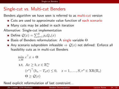
Single-cut vs. Multi-cut Benders

Benders algorithm we have seen is referred to as multi-cut version

Cuts are used to approximate value function of each scenario

Many cuts may be added in each iteration

Alternative: Single-cut implementation

Define Q(x) =∑S

s=1 psQs(x)

Basis of Benders reformulation: A single variable Θ

Any scenario subproblem infeasible ⇒ Q(x) not defined: Enforce allfeasibility cuts as in multi-cut Benders

minx,Θ

c>x+ Θ

s.t. Ax ≥ b, x ∈ Rn1+

(rs)>(hs − Tsx) ≤ 0, s = 1, . . . , S, rs ∈ XR(Πs)

Θ ≥ Q(x)

Need explicit reformulation of last constraint...Jim Luedtke (UW-Madison) Benders Decomposition Lecture Notes 24 / 33

Single-cut Benders

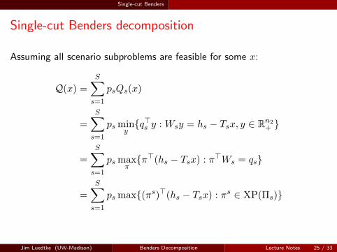
Single-cut Benders decomposition

Assuming all scenario subproblems are feasible for some x:

Q(x) =

S∑s=1

psQs(x)

=

S∑s=1

ps minyq>s y : Wsy = hs − Tsx, y ∈ Rn2

+

=

S∑s=1

ps maxππ>(hs − Tsx) : π>Ws = qs

=

S∑s=1

ps max(πs)>(hs − Tsx) : πs ∈ XP(Πs)


Single-cut Benders

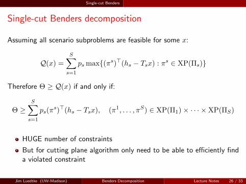
Single-cut Benders decomposition

Assuming all scenario subproblems are feasible for some x:

Q(x) =

S∑s=1

ps max(πs)>(hs − Tsx) : πs ∈ XP(Πs)

Therefore Θ ≥ Q(x) if and only if:

Θ ≥S∑s=1

ps(πs)>(hs − Tsx), (π1, . . . , πS) ∈ XP(Π1)× · · · ×XP(ΠS)

HUGE number of constraints

But for cutting plane algorithm only need to be able to efficiently finda violated constraint


Single-cut Benders

Single-cut Benders master problem

Master problem after adding t optimality cuts

minx,Θ

c>x+ Θ

s.t. Ax ≥ b, x ∈ Rn1+

Θ ≥ dk − c>k x, k = 1, . . . , t

(rs)>(hs − Tsx) ≤ 0, s = 1, . . . , S, rs ∈ Rs

The constraints Θ ≥ dk − c>k x, k = 1, . . . , t are just a compact way ofwriting a subset of these constraints:

Θ ≥S∑s=1

ps(πs)>(hs − Tsx), (π1, . . . , πS) ∈ XP(Π1)× · · · ×XP(ΠS)


Single-cut Benders

Single-cut Benders master problem

Let (x, Θ) be a master problem optimal solution

Solve all scenario subproblems for this x

If any one of them is infeasible: Add feasibility cut(s)

Else if Θ ≥∑S

s=1 psQs(x): Solution is feasible, hence optimal

Else:

Let πs be optimal extreme point dual solution, s = 1, . . . , SAdd following cut which is violated by (x, Θ):

Θ ≥S∑

s=1

ps(πs)>(hs − Tsx) := dt+1 − c>t+1x

where dt+1 =∑S

s=1 ps(πs)>hs and ct+1 =

∑Ss=1(πs)>Ts


Single-cut Benders

Single-cut vs. Multi-cut Benders

Single-cut Benders

Fewer variables and optimality cuts ⇒ Master problem typically solvesfaster

Must solve all subproblems to generate an optimality cut

Multi-cut Benders

Many cuts added per iteration ⇒ Typically converges in many fewerinterations

Master problem may become large and slow to solve

Do not need to solve all subproblems every iteration


Cut Selection

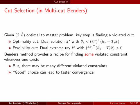
Cut Selection (in Multi-cut Benders)

Given (x, θ) optimal to master problem, key step is finding a violated cut:

Optimality cut: Dual solution πs with θs < (πs)>(hs − Tsx)

Feasibility cut: Dual extreme ray rs with (rs)>(hs − Tsx) > 0

Benders method provides a recipe for finding some violated constraintwhenever one exists

But, there may be many different violated constraints

“Good” choice can lead to faster convergence


Cut Selection

Alternative Cut Generation Problem

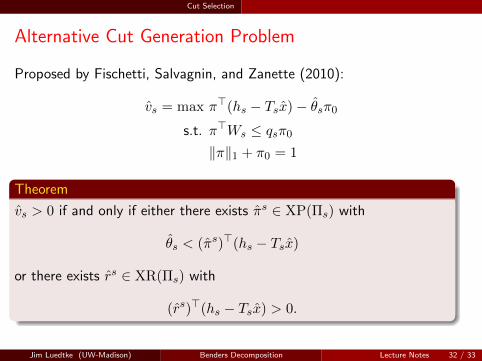
Proposed by Fischetti, Salvagnin, and Zanette (2010):

vs = max π>(hs − Tsx)− θsπ0

s.t. π>Ws ≤ qsπ0

‖π‖1 + π0 = 1

Theorem

vs > 0 if and only if either there exists πs ∈ XP(Πs) with

θs < (πs)>(hs − Tsx)

or there exists rs ∈ XR(Πs) with

(rs)>(hs − Tsx) > 0.


Cut Selection

Alternative Cut Generation Problem

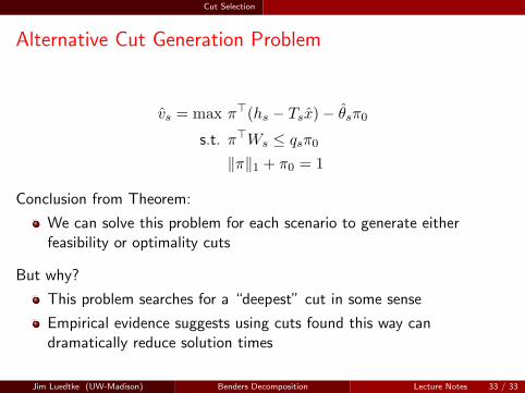
vs = max π>(hs − Tsx)− θsπ0

s.t. π>Ws ≤ qsπ0

‖π‖1 + π0 = 1

Conclusion from Theorem:

We can solve this problem for each scenario to generate eitherfeasibility or optimality cuts

But why?

This problem searches for a “deepest” cut in some sense

Empirical evidence suggests using cuts found this way candramatically reduce solution times


Documents

Benders Decomposition for Solving Two-stage Stochastic ... · Benders Decomposition for Solving Two-stage Stochastic Optimization Models IMA New Directions Short Course on Mathematical