REDES BAYESIANAS APLICADAS A UN MODELO CFD DEL ENTORNO DE ... · PDF filebabilidad de lluvia con datos incompletos. El objetivo de este estudio fue determinar la distribución de la

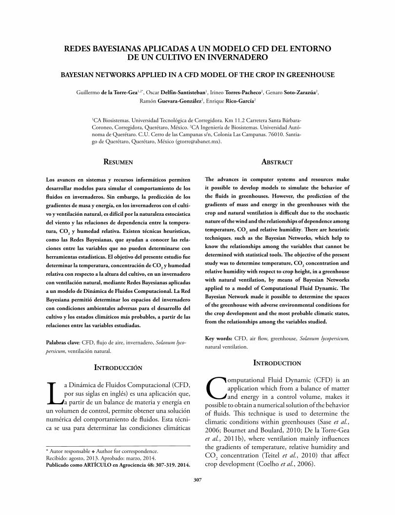
307

REDES BAYESIANAS APLICADAS A UN MODELO CFD DEL ENTORNO DE UN CULTIVO EN INVERNADERO

BAYESIAN NETWORKS APPLIED IN A CFD MODEL OF THE CROP IN GREENHOUSE

Guillermo de la Torre-Gea1,2*, Oscar Delfín-Santisteban1, Irineo Torres-Pacheco2, Genaro Soto-Zarazúa2, Ramón Guevara-González2, Enrique Rico-García2

1CA Biosistemas. Universidad Tecnológica de Corregidora. Km 11.2 Carretera Santa Bárbara-Coroneo, Corregidora, Querétaro, México. 2CA Ingeniería de Biosistemas. Universidad Autó-noma de Querétaro. C.U. Cerro de las Campanas s/n, Colonia Las Campanas. 76010. Santia-go de Querétaro, Querétaro, México ([email protected]).

Resumen

Los avances en sistemas y recursos informáticos permiten desarrollar modelos para simular el comportamiento de los fluidos en invernaderos. Sin embargo, la predicción de los gradientes de masa y energía, en los invernaderos con el culti-vo y ventilación natural, es difícil por la naturaleza estocástica del viento y las relaciones de dependencia entre la tempera-tura, CO2 y humedad relativa. Existen técnicas heurísticas, como las Redes Bayesianas, que ayudan a conocer las rela-ciones entre las variables que no pueden determinarse con herramientas estadísticas. El objetivo del presente estudio fue determinar la temperatura, concentración de CO2 y humedad relativa con respecto a la altura del cultivo, en un invernadero con ventilación natural, mediante Redes Bayesianas aplicadas a un modelo de Dinámica de Fluidos Computacional. La Red Bayesiana permitió determinar los espacios del invernadero con condiciones ambientales adversas para el desarrollo del cultivo y los estados climáticos más probables, a partir de las relaciones entre las variables estudiadas.

Palabras clave: CFD, flujo de aire, invernadero, Solanum lyco-persicum, ventilación natural.

IntRoduccIón

La Dinámica de Fluidos Computacional (CFD, por sus siglas en inglés) es una aplicación que, a partir de un balance de materia y energía en

un volumen de control, permite obtener una solución numérica del comportamiento de fluidos. Esta técni-ca se usa para determinar las condiciones climáticas

* Autor responsable v Author for correspondence.Recibido: agosto, 2013. Aprobado: marzo, 2014.Publicado como ARTÍCULO en Agrociencia 48: 307-319. 2014.

AbstRAct

The advances in computer systems and resources make it possible to develop models to simulate the behavior of the fluids in greenhouses. However, the prediction of the gradients of mass and energy in the greenhouses with the crop and natural ventilation is difficult due to the stochastic nature of the wind and the relationships of dependence among temperature, CO2 and relative humidity. There are heuristic techniques, such as the Bayesian Networks, which help to know the relationships among the variables that cannot be determined with statistical tools. The objective of the present study was to determine temperature, CO2 concentration and relative humidity with respect to crop height, in a greenhouse with natural ventilation, by means of Bayesian Networks applied to a model of Computational Fluid Dynamic. The Bayesian Network made it possible to determine the spaces of the greenhouse with adverse environmental conditions for the crop development and the most probable climatic states, from the relationships among the variables studied.

Key words: CFD, air flow, greenhouse, Solanum lycopersicum, natural ventilation.

IntRoductIon

Computational Fluid Dynamic (CFD) is an application which from a balance of matter and energy in a control volume, makes it

possible to obtain a numerical solution of the behavior of fluids. This technique is used to determine the climatic conditions within greenhouses (Sase et al., 2006; Bournet and Boulard, 2010; De la Torre-Gea et al., 2011b), where ventilation mainly influences the gradients of temperature, relative humidity and CO2 concentration (Teitel et al., 2010) that affect crop development (Coelho et al., 2006).

AGROCIENCIA, 1 de abril - 15 de mayo, 2014

VOLUMEN 48, NÚMERO 3308

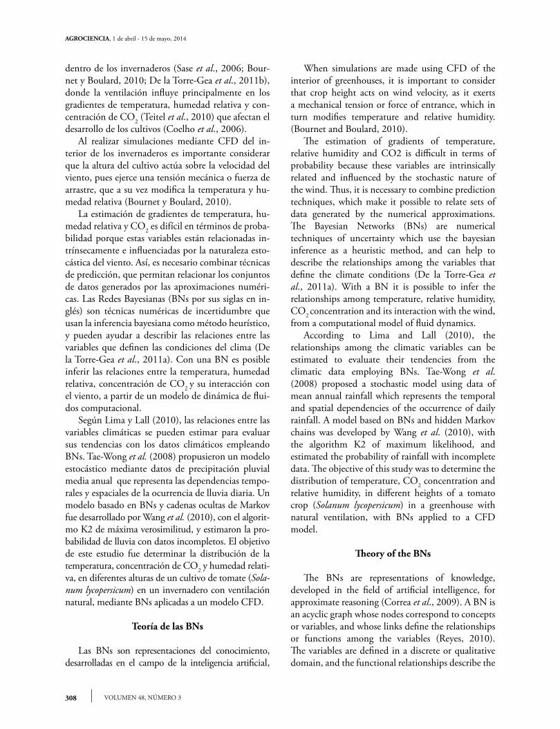
dentro de los invernaderos (Sase et al., 2006; Bour-net y Boulard, 2010; De la Torre-Gea et al., 2011b), donde la ventilación influye principalmente en los gradientes de temperatura, humedad relativa y con-centración de CO2 (Teitel et al., 2010) que afectan el desarrollo de los cultivos (Coelho et al., 2006).

Al realizar simulaciones mediante CFD del in-terior de los invernaderos es importante considerar que la altura del cultivo actúa sobre la velocidad del viento, pues ejerce una tensión mecánica o fuerza de arrastre, que a su vez modifica la temperatura y hu-medad relativa (Bournet y Boulard, 2010).

La estimación de gradientes de temperatura, hu-medad relativa y CO2 es difícil en términos de proba-bilidad porque estas variables están relacionadas in-trínsecamente e influenciadas por la naturaleza esto-cástica del viento. Así, es necesario combinar técnicas de predicción, que permitan relacionar los conjuntos de datos generados por las aproximaciones numéri-cas. Las Redes Bayesianas (BNs por sus siglas en in-glés) son técnicas numéricas de incertidumbre que usan la inferencia bayesiana como método heurístico, y pueden ayudar a describir las relaciones entre las variables que definen las condiciones del clima (De la Torre-Gea et al., 2011a). Con una BN es posible inferir las relaciones entre la temperatura, humedad relativa, concentración de CO2 y su interacción con el viento, a partir de un modelo de dinámica de flui-dos computacional.

Según Lima y Lall (2010), las relaciones entre las variables climáticas se pueden estimar para evaluar sus tendencias con los datos climáticos empleando BNs. Tae-Wong et al. (2008) propusieron un modelo estocástico mediante datos de precipitación pluvial media anual que representa las dependencias tempo-rales y espaciales de la ocurrencia de lluvia diaria. Un modelo basado en BNs y cadenas ocultas de Markov fue desarrollado por Wang et al. (2010), con el algorit-mo K2 de máxima verosimilitud, y estimaron la pro-babilidad de lluvia con datos incompletos. El objetivo de este estudio fue determinar la distribución de la temperatura, concentración de CO2 y humedad relati-va, en diferentes alturas de un cultivo de tomate (Sola-num lycopersicum) en un invernadero con ventilación natural, mediante BNs aplicadas a un modelo CFD.

Teoría de las BNs

Las BNs son representaciones del conocimiento, desarrolladas en el campo de la inteligencia artificial,

When simulations are made using CFD of the interior of greenhouses, it is important to consider that crop height acts on wind velocity, as it exerts a mechanical tension or force of entrance, which in turn modifies temperature and relative humidity. (Bournet and Boulard, 2010).

The estimation of gradients of temperature, relative humidity and CO2 is difficult in terms of probability because these variables are intrinsically related and influenced by the stochastic nature of the wind. Thus, it is necessary to combine prediction techniques, which make it possible to relate sets of data generated by the numerical approximations. The Bayesian Networks (BNs) are numerical techniques of uncertainty which use the bayesian inference as a heuristic method, and can help to describe the relationships among the variables that define the climate conditions (De la Torre-Gea et al., 2011a). With a BN it is possible to infer the relationships among temperature, relative humidity, CO2 concentration and its interaction with the wind, from a computational model of fluid dynamics.

According to Lima and Lall (2010), the relationships among the climatic variables can be estimated to evaluate their tendencies from the climatic data employing BNs. Tae-Wong et al. (2008) proposed a stochastic model using data of mean annual rainfall which represents the temporal and spatial dependencies of the occurrence of daily rainfall. A model based on BNs and hidden Markov chains was developed by Wang et al. (2010), with the algorithm K2 of maximum likelihood, and estimated the probability of rainfall with incomplete data. The objective of this study was to determine the distribution of temperature, CO2 concentration and relative humidity, in different heights of a tomato crop (Solanum lycopersicum) in a greenhouse with natural ventilation, with BNs applied to a CFD model.

Theory of the BNs

The BNs are representations of knowledge, developed in the field of artificial intelligence, for approximate reasoning (Correa et al., 2009). A BN is an acyclic graph whose nodes correspond to concepts or variables, and whose links define the relationships or functions among the variables (Reyes, 2010). The variables are defined in a discrete or qualitative domain, and the functional relationships describe the

309DE LA TORRE-GEA et al.


para el razonamiento aproximado (Correa et al., 2009). Una BN es un gráfico acíclico cuyos nodos corresponden a conceptos o variables, y cuyos enlaces definen las relaciones o funciones entre las variables (Reyes, 2010). Las variables se definen en un domi-nio discreto o cualitativo, y las relaciones funcionales describen las inferencias causales expresadas en tér-minos de probabilidades condicionales (Ecuación 1).

P x x P x padres xn i ii

n

11

,..., |b g b gd i==∏ (1)

Las BNs se pueden usar para identificar las rela-ciones entre las variables anteriormente indetermi-nadas o para describir y cuantificar estas relaciones, incluso con un conjunto de datos incompletos. Los algoritmos de solución de las BNs permiten calcular la distribución de probabilidad esperada de las varia-bles de salida. El resultado de este cálculo es depen-diente de la distribución de probabilidad de las varia-bles de entrada. Las BNs pueden ser percibidas como una distribución de probabilidades conjunta de una colección de variables aleatorias discretas (Gámez et al., 2011). La probabilidad a priori P (cj) es la probabilidad de que una muestra xi pertenezca a la clase CJ, defi-nida sin información sobre sus valores característicos (Ecuación 2).

P(cj / xi)=P (xi / cj) P (cj) / ∑P(xi / ck) P(ck) (2)

Las máquinas de aprendizaje, en la inteligencia artificial, están relacionadas estrechamente con la mi-nería de datos, los métodos de clasificación o agru-pamiento en estadística, el razonamiento inductivo y el reconocimiento de patrones. Los métodos estadís-ticos de aprendizaje automático se pueden aplicar al marco de la estadística bayesiana; sin embargo, la má-quina de aprendizaje puede emplear una variedad de técnicas de clasificación para producir otros modelos de BNs (Garrote et al., 2007). El objetivo del apren-dizaje mediante una BN es encontrar el arreglo que describa mejor a los datos observados. El número de estructuras posibles de grafos acíclicos directos para la búsqueda es exponencial al número de variables en el dominio, definido por la Ecuación 3:

f n c f n iin i n

in i( ) ( )( )= − −=

+ −∑ 11

1 2b g (3)

causal inferences expressed in terms of conditional probabilities (Equation 1).

P x x P x padres xn i ii

n

11

,..., |b g b gd i==∏ (1)

The BNs can be used to identify the relationships among the previously undetermined variables or to describe and quantify these relationships, even with a set of incomplete data. The algorithms of solution of the BNs permit the calculation of the distribution of probability expected from the output variables. The result of this calculation is dependent on the distribution of probability of the input variables. The BNs can be perceived as a distribution of joint probabilities of a collection of discrete random variables (Gámez et al., 2011).

The a priori probability P (cj) is a probability that a sample xi belongs to the class Cj, defined without information of its characteristic values (Equation 2).

P(cj / xi)=P (xi / cj) P (cj) / ∑P(xi / ck) P(ck) (2)

The learning machines in artificial intelligence are closely related to the data mining, classification or grouping methods in statistics, inductive reasoning and pattern recognition. Statistical methods of automatic learning can be applied to the framework of Bayesian statistics. However, the learning machine may employ a variety of classification techniques to produce other BNs models (Garrote et al., 2007). The objective of learning by means of a BN is to find the arrangement that best describes the observed data. The number of possible structures of direct acyclic graphs for the search is exponential to the number of variables in the domain, defined by equation 3.

f n c f n iin i n

in i( ) ( )( )= − −=

+ −∑ 11

1 2b g (3)

The algorithm K2 is the most representative method among the approximations of “search and result”. The algorithm begins by assigning each variable without parents. Next, it incrementally adds the parents to the present variable which increases its punctuation in the resulting structure. When any addition of a single mother cannot increase the count, it stops adding parents to the variable. If we consider



El algoritmo K2 es el método más representativo entre las aproximaciones de “búsqueda y resultado”. El algoritmo comienza asignando a cada variable sin padres. Luego agrega de manera incremental los pa-dres a la variable actual que aumenta su puntuación en la estructura resultante. Cuando cualquier adición de una madre soltera no puede aumentar la cuenta, deja de agregar padres a la variable. Si se considera un valor conocido de antemano de alguna de las va-riables, el espacio de búsqueda bajo esta restricción es menor que el espacio de la estructura entera. Si el orden de las variables es desconocido, puede realizar-se la búsqueda en los ordenamientos posibles (Hrus-chka et al., 2007).

mAteRIAles y métodos

Caracterización del flujo de aire y variables de estado

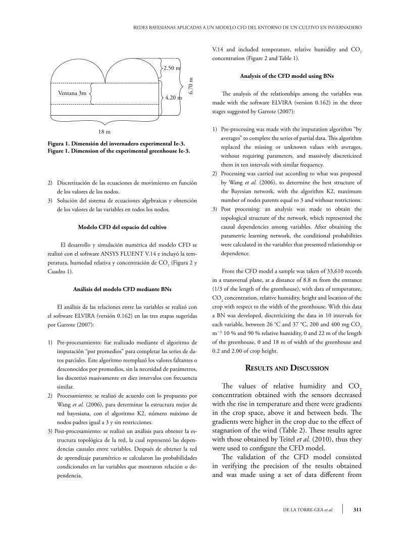
En el invernadero experimental Ie3 de la Universidad Autó-noma de Querétaro, campus Amazcala, se realizaron muestreos entre el 21 y 25 de agosto de 2011, para determinar las condi-ciones iniciales del modelo CFD y entre el 15 y 22 de abril de 2012, para validar el modelo CFD. El invernadero Gótico tiene 432 m2, está dividido en dos naves, cada una de 9×24 m, con altura a la canaleta de 4.20 m y 6.70 m a la cumbrera (2.50 m de cumbrera), sin ventanas cenitales sólo laterales de tipo enrollable, de 3×9 m a la cara frontal y posterior y de 3×16 m a los costados (Figura 1). Su orientación fue de norte-sur, igual que los camello-nes del cultivo. Solanum lycopersicum se cultivó con densidad de 2.5 plantas m-2, anchura de los camellones del cultivo de 60 cm, altura de 2 m y pasillo de 1 m entre camellones.

Los datos incluyeron la temperatura, humedad relativa, con-centración de CO2 y velocidad del viento. Las mediciones se rea-lizaron a 1 y 3 m de altura sobre al suelo, cada 4 min, con un sensor tipo LM335 para la temperatura y humedad relativa y con un sensor modelo FYA600CO2H para la concentración de CO2. La velocidad y dirección del viento fueron medidas cada 2 s con anemómetros omnidireccionales, con intervalo entre 0 y 20 m s-1 y precisión de 0.03 m s-1.

Metodología para el desarrollo del modelo CFD

La metodología para desarrollar el modelo CFD fue pro-puesta por Rico-García (2008), en tres etapas:

1) Discretización del flujo continuo: las variables de campo se aproximaron a un número finito de valores en puntos llama-dos nodos.

an already known value of one of the variables, the search space under this restriction is lower than the space of the entire structure. If the order of the variables is unknown, the search can be carried out in the possible orderings (Hruschka et al., 2007).

mAteRIAls And methods

Characterization of air flow and state variables

In the experimental greenhouse Ie3 of the Querétaro Autonomous University, Amazcala campus, samplings were carried out between August 21 and 25 of 2011 to determine the initial conditions of the CFD model and between April 15 and 22 of 2012, to validate the CFD model. The Gothic greenhouse has 432 m2, and is divided into two aisles, each one with 9×24 m, with a height to the gutter of 4.20 m and 6.70 m to the ridge (2.50 m of ridge), without zenithal windows, only roll-up lateral windows, of 3×9 m to the front and back ends and 3×16 m at the sides (Figure 1). It had a north-south orientation, as well as raised crop beds. Solanum lycopersicum was cultivated with a density of 2.5 plants m-2, width of the crop beds 60 cm, height of 2 m and aisles between beds of 1 m.

The data include temperature, relative humidity, concentration of CO2 and wind velocity. The measurements were made at 1 and 3 m height over the ground, every 4 min, with a type LM335 sensor for temperature and relative humidity and with a FYA600CO2H for the CO2 concentration. Wind velocity and direction were measured every 2 s with omni-directional anemometers, with an interval between 0 and 20 m s-1 and precision of 0.03 m s-1.

Methodology for the development of the CFD model

The methodology to develop the CFD model was proposed by Rico-García (2008), in three stages:

1) Discretization of the continuous flow: the field variables approximated a finite number of values in points called nodes.

2) Discretization of the equations of movement as a function of the values of the nodes.

3) Solution of the system of algebraic equations and obtaining of the values of the variables in all of the nodes.

CFD model of the crop space

The development and numerical simulation of the CFD model was carried out with the software ANSYS FLUENT



Figura 1. Dimensión del invernadero experimental Ie-3.Figure 1. Dimension of the experimental greenhouse Ie-3.

2.50 m

Ventana 3m

18 m

4.20 m

6.70

m2) Discretización de las ecuaciones de movimiento en función

de los valores de los nodos.3) Solución del sistema de ecuaciones algebraicas y obtención

de los valores de las variables en todos los nodos.

Modelo CFD del espacio del cultivo

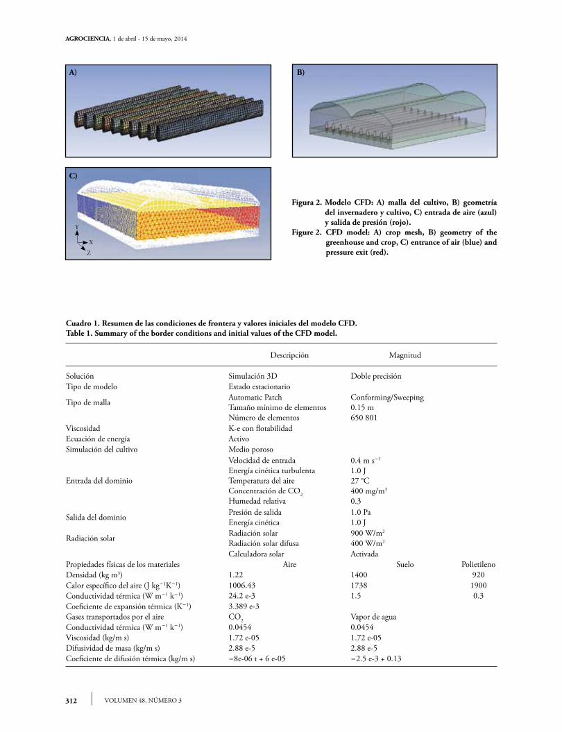
El desarrollo y simulación numérica del modelo CFD se realizó con el software ANSYS FLUENT V.14 e incluyó la tem-peratura, humedad relativa y concentración de CO2 (Figura 2 y Cuadro 1).

Análisis del modelo CFD mediante BNs

El análisis de las relaciones entre las variables se realizó con el software ELVIRA (versión 0.162) en las tres etapas sugeridas por Garrote (2007):

1) Pre-procesamiento: fue realizado mediante el algoritmo de imputación “por promedios” para completar las series de da-tos parciales. Este algoritmo reemplazó los valores faltantes o desconocidos por promedios, sin la necesidad de parámetros, los discretizó masivamente en diez intervalos con frecuencia similar.

2) Procesamiento: se realizó de acuerdo con lo propuesto por Wang et al. (2006), para determinar la estructura mejor de red bayesiana, con el algoritmo K2, número máximo de nodos padres igual a 3 y sin restricciones.

3) Post-procesamiento: se realizó un análisis para obtener la es-tructura topológica de la red, la cual representó las depen-dencias causales entre variables. Después de obtener la red de aprendizaje paramétrico se calcularon las probabilidades condicionales en las variables que mostraron relación o de-pendencia.

V.14 and included temperature, relative humidity and CO2 concentration (Figure 2 and Table 1).

Analysis of the CFD model using BNs

The analysis of the relationships among the variables was made with the software ELVIRA (version 0.162) in the three stages suggested by Garrote (2007):

1) Pre-processing was made with the imputation algorithm “by averages” to complete the series of partial data. This algorithm replaced the missing or unknown values with averages, without requiring parameters, and massively discreticized them in ten intervals with similar frequency.

2) Processing was carried out according to what was proposed by Wang et al. (2006), to determine the best structure of the Bayesian network, with the algorithm K2, maximum number of nodes parents equal to 3 and without restrictions.

3) Post processing: an analysis was made to obtain the topological structure of the network, which represented the causal dependencies among variables. After obtaining the parametric learning network, the conditional probabilities were calculated in the variables that presented relationship or dependence.

From the CFD model a sample was taken of 33,610 records in a transversal plane, at a distance of 8.8 m from the entrance (1/3 of the length of the greenhouse), with data of temperature, CO2 concentration, relative humidity, height and location of the crop with respect to the width of the greenhouse. With this data a BN was developed, discreticizing the data in 10 intervals for each variable, between 26 °C and 37 °C, 200 and 400 mg CO2 m-3, 10 % and 90 % relative humidity, 0 and 22 m of the length of the greenhouse, 0 and 18 m of width of the greenhouse and 0.2 and 2.00 of crop height.

Results And dIscussIon

The values of relative humidity and CO2 concentration obtained with the sensors decreased with the rise in temperature and there were gradients in the crop space, above it and between beds. The gradients were higher in the crop due to the effect of stagnation of the wind (Table 2). These results agree with those obtained by Teitel et al. (2010), thus they were used to configure the CFD model.

The validation of the CFD model consisted in verifying the precision of the results obtained and was made using a set of data different from



Figura 2. Modelo CFD: A) malla del cultivo, B) geometría del invernadero y cultivo, C) entrada de aire (azul) y salida de presión (rojo).

Figure 2. CFD model: A) crop mesh, B) geometry of the greenhouse and crop, C) entrance of air (blue) and pressure exit (red).

Cuadro 1. Resumen de las condiciones de frontera y valores iniciales del modelo CFD.Table 1. Summary of the border conditions and initial values of the CFD model.

Descripción Magnitud

Solución Simulación 3D Doble precisiónTipo de modelo Estado estacionario

Tipo de malla Automatic Patch Tamaño mínimo de elementosNúmero de elementos

Conforming/Sweeping0.15 m650 801

Viscosidad K-e con flotabilidad Ecuación de energía ActivoSimulación del cultivo Medio poroso

Entrada del dominio

Velocidad de entradaEnergía cinética turbulentaTemperatura del aireConcentración de CO2Humedad relativa

0.4 m s-1

1.0 J27 °C400 mg/m3

0.3

Salida del dominio Presión de salidaEnergía cinética

1.0 Pa1.0 J

Radiación solar Radiación solar Radiación solar difusa

900 W/m2

400 W/m2

Calculadora solar ActivadaPropiedades físicas de los materiales Aire Suelo PolietilenoDensidad (kg m3) 1.22 1400 920Calor específico del aire (J kg-1K-1) 1006.43 1738 1900Conductividad térmica (W m-1 k-1) 24.2 e-3 1.5 0.3Coeficiente de expansión térmica (K-1) 3.389 e-3 Gases transportados por el aire CO2 Vapor de aguaConductividad térmica (W m-1 k-1) 0.0454 0.0454 Viscosidad (kg/m s) 1.72 e-05 1.72 e-05 Difusividad de masa (kg/m s) 2.88 e-5 2.88 e-5 Coeficiente de difusión térmica (kg/m s) -8e-06 t + 6 e-05 -2.5 e-3 + 0.13

Y

X

Z

B)

C)

A)



Del modelo CFD se tomó una muestra de 33,610 registros en un plano transversal, a una distancia de 8.8 m de la entrada (1/3 de la longitud del invernadero), con datos de temperatura, concentración de CO2, humedad relativa, altura y ubicación del cultivo con respecto a la anchura del invernadero. Con ellos se desarrolló una BN, discretizando los datos en 10 intervalos para cada variable, entre 26 °C y 37 °C, 200 y 400 mg CO2 m-3, 10% y 90% de humedad relativa, 0 y 22 m de la longitud del invernadero, 0 y 18 m de anchura del invernadero y 0.2 y 2.00 m de altura del cultivo.

ResultAdos y dIscusIón

Los valores de humedad relativa y concentración de CO2 obtenidos con los sensores disminuyeron con el aumento de la temperatura y existieron gradientes en el espacio del cultivo, encima de él y entre los ca-mellones. Los gradientes fueron mayores en el cultivo debido al efecto del estancamiento del viento (Cua-dro 2). Estos resultados coinciden con los obtenidos por Teitel et al. (2010), por lo cual se usaron para configurar el modelo CFD.

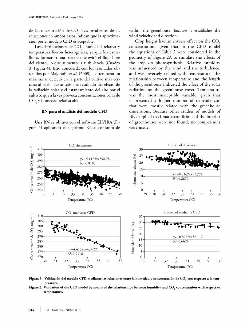
La validación del modelo CFD consistió en veri-ficar la exactitud de los resultados obtenidos y se rea-lizó a través de un conjunto de datos diferente al de las mediciones obtenidas para definir las condiciones iniciales y de frontera del modelo desarrollado. Una prueba de significancia se aplicó mediante análisis de regresión lineal, de las relaciones entre humedad y CO2 con respecto a la temperatura, en condiciones climáticas similares (Figura 3).

La regresión lineal mostró que la concentración de CO2 y humedad relativa en el modelo CFD son similares con el conjunto de datos medidos, con 5 % de diferencia en la ordenada al origen en la ecuación de la humedad relativa, y 39 mg m-3 en la ecuación

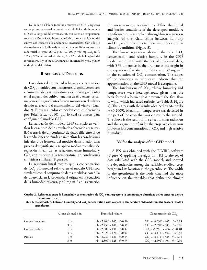
Cuadro 2. Relaciones entre la humedad y concentración de CO2 con respecto a la temperatura obtenidas de los sensores dentro de un invernadero.

Table 2. Relationships between humidity and CO2 concentration with respect to temperature obtained from the sensors inside a greenhouse.

Alturas de medición Humedad relativa Concentración de CO2

Cultivo inmaduro 1 m H=-2.40T + 105, r2=0.90 CO2 = -4.03T + 407, r2 = 0.883 m H=-2.25T + 100, r2=0.89 CO2 = -2.39T + 383, r2 = 0.86

Cultivo maduro 1 m H=-2.50T + 130, r2=0.97 CO2 = -5.26 T + 436, r2 =0 .813 m H=-2.62T + 121, r2=0.97 CO2 = -4.11T + 442, r2 = 0.81

Pasillos 1 m H=-3.23T + 131, r2=0.94 CO2 = -3.41T + 385, r2 = 0.963 m H=-2.80T + 128, r2=0.95 CO2 = -2.69T + 404, r2 = 0.90

the measurements obtained to define the initial and border conditions of the developed model. A significance test was applied, through linear regression analysis, of the relationships between humidity and C02 with respect to temperature, under similar climatic conditions (Figure 3).

The linear regression showed that the CO2 concentration and relative humidity in the CFD model are similar with the set of measured data, with 5 % difference in the ordinate at the origin in the equation of relative humidity, and 39 mg m-3 in the equation of CO2 concentration. The slopes of the equations in both cases indicate that the approximation by the CFD model is acceptable.

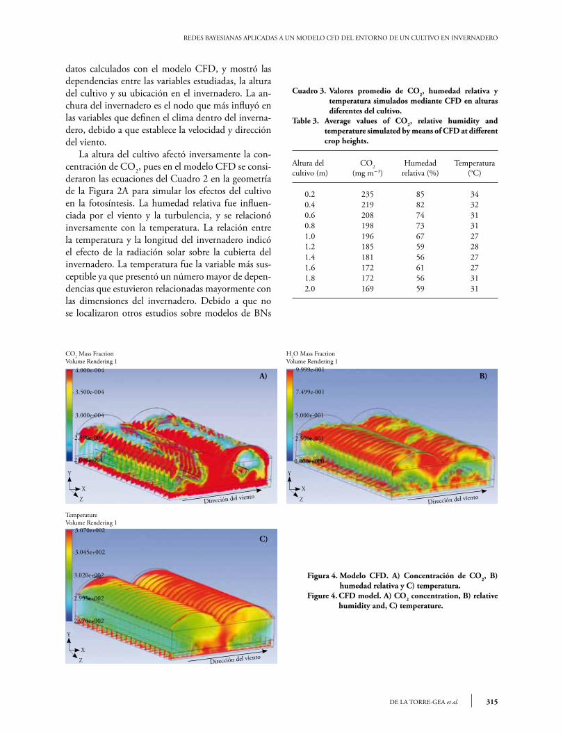
The distributions of CO2, relative humidity and temperature were heterogeneous, given that the beds formed a barrier that prevented the free flow of wind, which increased turbulence (Table 3, Figure 4). This agrees with the results obtained by Majdoubi et al.(2009). Maximum temperature was detected in the part of the crop that was closest to the ground. The above is the result of the effect of solar radiation and the stagnation of air by the crop, which in turn provokes low concentrations of CO2 and high relative humidity.

BN for the analysis of the CFD model

A BN was obtained with the ELVIRA software (Figure 5) applying the algorithm K2 to the set of data calculated with the CFD model, and showed the dependencies among the variables studied, crop height and its location in the greenhouse. The width of the greenhouse is the node that had the most influence on the variables that define the climate



de la concentración de CO2. Las pendientes de las ecuaciones en ambos casos indican que la aproxima-ción por el modelo CFD es aceptable.

Las distribuciones de CO2, humedad relativa y temperatura fueron heterogéneas, ya que los came-llones formaron una barrera que evitó el flujo libre del viento, lo que aumentó la turbulencia (Cuadro 3, Figura 4). Esto concuerda con los resultados ob-tenidos por Majdoubi et al. (2009). La temperatura máxima se detectó en la parte del cultivo más cer-cana al suelo. Lo anterior es resultado del efecto de la radiación solar y el estancamiento del aire por el cultivo, que a la vez provoca concentraciones bajas de CO2 y humedad relativa alta.

BN para el análisis del modelo CFD

Una BN se obtuvo con el software ELVIRA (Fi-gura 5) aplicando el algoritmo K2 al conjunto de

Figura 3. Validación del modelo CFD mediante las relaciones entre la humedad y concentración de CO2 con respecto a la tem-peratura.

Figure 3. Validation of the CFD model by means of the relationships between humidity and CO2 concentration with respect to temperature.

310

300

290

280

270

260

250

24030 31 32 33 34 35 36 37 38

Con

cent

raci

ón d

e C

O2 (

mg

m

3 )

Temperatura (°C)

y=4.1123x+398.78R2=0.8105

30

25

20

15

10

5

030 31 32 33 34 35 36 3729

Hum

edad

rel

ativ

a (%

)

Temperatura (°C)

y=0.9167x+51.774R2=0.8679

310

305300

295

290285280

275

30 31 32 33 34 35 36 37

Con

cent

raci

ón d

e C

O2 (

mg

m

3 )

Temperatura (°C)

y=4.4152x+437.22R2=0.9116

270

35

30

25

20

15

10

5

30 31 32 33 34 35 36 37

Temperatura (°C)

y=0.8287x+56.117R2=0.6674

0

Hum

edad

rel

ativ

a (%

)

CO2 de sensores

CO2 mediante CFD

Humedad de sensores

Humedad mediante CFD

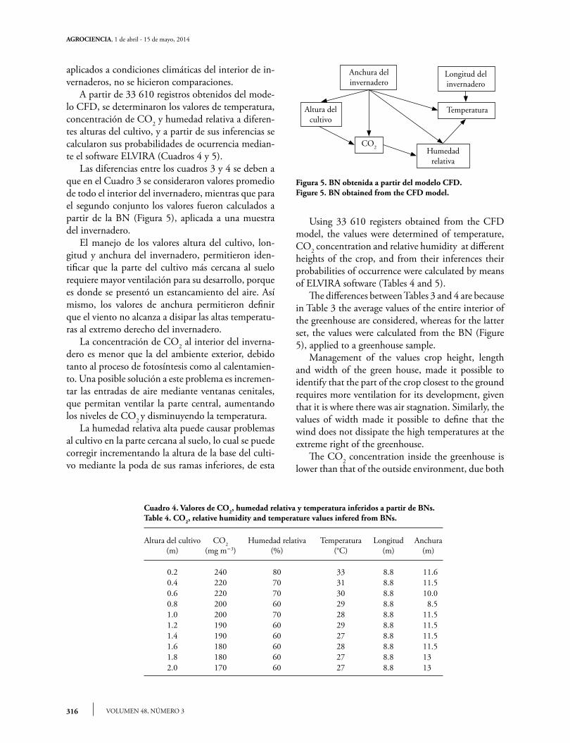
within the greenhouse, because it establishes the wind velocity and direction.

Crop height had an inverse effect on the CO2 concentration, given that in the CFD model the equations of Table 2 were considered in the geometry of Figure 2A to simulate the effects of the crop on photosynthesis. Relative humidity was influenced by the wind and the turbulence, and was inversely related with temperature. The relationship between temperature and the length of the greenhouse indicated the effect of the solar radiation on the greenhouse cover. Temperature was the most susceptible variable, given that it presented a higher number of dependencies that were mostly related with the greenhouse dimensions. Because other studies of models of BNs applied to climatic conditions of the interior of greenhouses were not found, no comparisons were made.



Cuadro 3. Valores promedio de CO2, humedad relativa y temperatura simulados mediante CFD en alturas diferentes del cultivo.

Table 3. Average values of CO2, relative humidity and temperature simulated by means of CFD at different crop heights.

Altura del cultivo (m)

CO2(mg m-3)

Humedad relativa (%)

Temperatura(°C)

0.2 235 85 340.4 219 82 320.6 208 74 310.8 198 73 311.0 196 67 271.2 185 59 281.4 181 56 271.6 172 61 271.8 172 56 312.0 169 59 31

Figura 4. Modelo CFD. A) Concentración de CO2, B) humedad relativa y C) temperatura.

Figure 4. CFD model. A) CO2 concentration, B) relative humidity and, C) temperature.

datos calculados con el modelo CFD, y mostró las dependencias entre las variables estudiadas, la altura del cultivo y su ubicación en el invernadero. La an-chura del invernadero es el nodo que más influyó en las variables que definen el clima dentro del inverna-dero, debido a que establece la velocidad y dirección del viento.

La altura del cultivo afectó inversamente la con-centración de CO2, pues en el modelo CFD se consi-deraron las ecuaciones del Cuadro 2 en la geometría de la Figura 2A para simular los efectos del cultivo en la fotosíntesis. La humedad relativa fue influen-ciada por el viento y la turbulencia, y se relacionó inversamente con la temperatura. La relación entre la temperatura y la longitud del invernadero indicó el efecto de la radiación solar sobre la cubierta del invernadero. La temperatura fue la variable más sus-ceptible ya que presentó un número mayor de depen-dencias que estuvieron relacionadas mayormente con las dimensiones del invernadero. Debido a que no se localizaron otros estudios sobre modelos de BNs

A) B)

C)

Dirección del vientoDirección del viento

Dirección del viento

Y

X

Z

Y

X

Z

Y

X

Z

H2O Mass FractionVolume Rendering 1

CO2 Mass FractionVolume Rendering 1

TemperatureVolume Rendering 1

4.000e-004

3.500e-004

3.000e-004

2.000e-004

2.500e-004

9.999e-001

7.499e-001

5.000e-001

2.500e-001

0.000e+000

3.070e+002

3.045e+002

3.020e+002

2.995e+002

2.970e+002



aplicados a condiciones climáticas del interior de in-vernaderos, no se hicieron comparaciones.

A partir de 33 610 registros obtenidos del mode-lo CFD, se determinaron los valores de temperatura, concentración de CO2 y humedad relativa a diferen-tes alturas del cultivo, y a partir de sus inferencias se calcularon sus probabilidades de ocurrencia median-te el software ELVIRA (Cuadros 4 y 5).

Las diferencias entre los cuadros 3 y 4 se deben a que en el Cuadro 3 se consideraron valores promedio de todo el interior del invernadero, mientras que para el segundo conjunto los valores fueron calculados a partir de la BN (Figura 5), aplicada a una muestra del invernadero.

El manejo de los valores altura del cultivo, lon-gitud y anchura del invernadero, permitieron iden-tificar que la parte del cultivo más cercana al suelo requiere mayor ventilación para su desarrollo, porque es donde se presentó un estancamiento del aire. Así mismo, los valores de anchura permitieron definir que el viento no alcanza a disipar las altas temperatu-ras al extremo derecho del invernadero.

La concentración de CO2 al interior del inverna-dero es menor que la del ambiente exterior, debido tanto al proceso de fotosíntesis como al calentamien-to. Una posible solución a este problema es incremen-tar las entradas de aire mediante ventanas cenitales, que permitan ventilar la parte central, aumentando los niveles de CO2 y disminuyendo la temperatura.

La humedad relativa alta puede causar problemas al cultivo en la parte cercana al suelo, lo cual se puede corregir incrementando la altura de la base del culti-vo mediante la poda de sus ramas inferiores, de esta

Figura 5. BN obtenida a partir del modelo CFD.Figure 5. BN obtained from the CFD model.

Anchura delinvernadero

Longitud delinvernadero

TemperaturaAltura delcultivo

CO2

Humedadrelativa

Cuadro 4. Valores de CO2, humedad relativa y temperatura inferidos a partir de BNs.Table 4. CO2, relative humidity and temperature values infered from BNs.

Altura del cultivo(m)

CO2(mg m-3)

Humedad relativa(%)

Temperatura(°C)

Longitud(m)

Anchura(m)

0.2 240 80 33 8.8 11.60.4 220 70 31 8.8 11.50.6 220 70 30 8.8 10.00.8 200 60 29 8.8 8.51.0 200 70 28 8.8 11.51.2 190 60 29 8.8 11.51.4 190 60 27 8.8 11.51.6 180 60 28 8.8 11.51.8 180 60 27 8.8 132.0 170 60 27 8.8 13

Using 33 610 registers obtained from the CFD model, the values were determined of temperature, CO2 concentration and relative humidity at different heights of the crop, and from their inferences their probabilities of occurrence were calculated by means of ELVIRA software (Tables 4 and 5).

The differences between Tables 3 and 4 are because in Table 3 the average values of the entire interior of the greenhouse are considered, whereas for the latter set, the values were calculated from the BN (Figure 5), applied to a greenhouse sample.

Management of the values crop height, length and width of the green house, made it possible to identify that the part of the crop closest to the ground requires more ventilation for its development, given that it is where there was air stagnation. Similarly, the values of width made it possible to define that the wind does not dissipate the high temperatures at the extreme right of the greenhouse.

The CO2 concentration inside the greenhouse is lower than that of the outside environment, due both



manera el viento podrá circular evitando el estanca-miento.

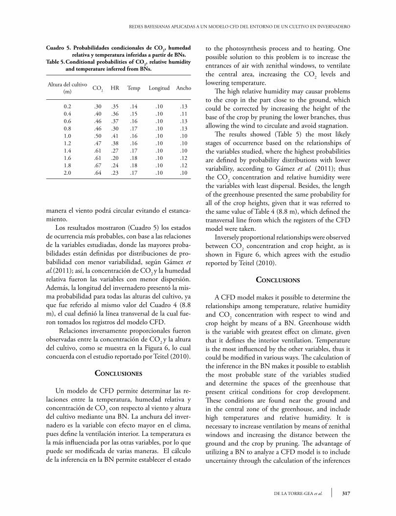
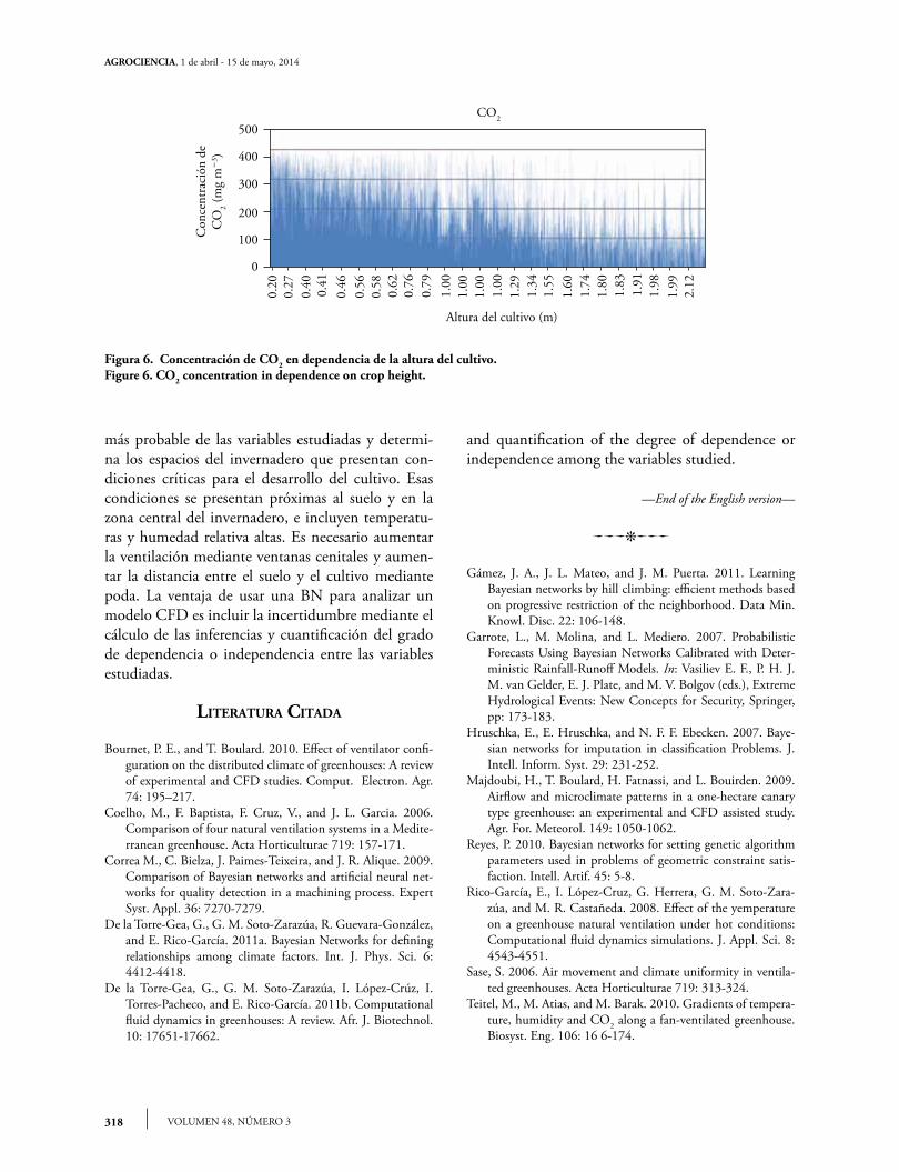
Los resultados mostraron (Cuadro 5) los estados de ocurrencia más probables, con base a las relaciones de la variables estudiadas, donde las mayores proba-bilidades están definidas por distribuciones de pro-babilidad con menor variabilidad, según Gámez et al.(2011); así, la concentración de CO2 y la humedad relativa fueron las variables con menor dispersión. Además, la longitud del invernadero presentó la mis-ma probabilidad para todas las alturas del cultivo, ya que fue referido al mismo valor del Cuadro 4 (8.8 m), el cual definió la línea transversal de la cual fue-ron tomados los registros del modelo CFD. Relaciones inversamente proporcionales fueron observadas entre la concentración de CO2 y la altura del cultivo, como se muestra en la Figura 6, lo cual concuerda con el estudio reportado por Teitel (2010).

conclusIones

Un modelo de CFD permite determinar las re-laciones entre la temperatura, humedad relativa y concentración de CO2 con respecto al viento y altura del cultivo mediante una BN. La anchura del inver-nadero es la variable con efecto mayor en el clima, pues define la ventilación interior. La temperatura es la más influenciada por las otras variables, por lo que puede ser modificada de varias maneras. El cálculo de la inferencia en la BN permite establecer el estado

Cuadro 5. Probabilidades condicionales de CO2, humedad relativa y temperatura inferidas a partir de BNs.

Table 5. Conditional probabilities of CO2, relative humidity and temperature inferred from BNs.

Altura del cultivo(m) CO2 HR Temp Longitud Ancho

0.2 .30 .35 .14 .10 .130.4 .40 .36 .15 .10 .110.6 .46 .37 .16 .10 .130.8 .46 .30 .17 .10 .131.0 .50 .41 .16 .10 .101.2 .47 .38 .16 .10 .101.4 .61 .27 .17 .10 .101.6 .61 .20 .18 .10 .121.8 .67 .24 .18 .10 .122.0 .64 .23 .17 .10 .10

to the photosynthesis process and to heating. One possible solution to this problem is to increase the entrances of air with zenithal windows, to ventilate the central area, increasing the CO2 levels and lowering temperature.

The high relative humidity may causar problems to the crop in the part close to the ground, which could be corrected by increasing the height of the base of the crop by pruning the lower branches, thus allowing the wind to circulate and avoid stagnation.

The results showed (Table 5) the most likely stages of occurrence based on the relationships of the variables studied, where the highest probabilities are defined by probability distributions with lower variability, according to Gámez et al. (2011); thus the CO2 concentration and relative humidity were the variables with least dispersal. Besides, the length of the greenhouse presented the same probability for all of the crop heights, given that it was referred to the same value of Table 4 (8.8 m), which defined the transversal line from which the registers of the CFD model were taken.

Inversely proportional relationships were observed between CO2 concentration and crop height, as is shown in Figure 6, which agrees with the estudio reported by Teitel (2010).

conclusIons

A CFD model makes it possible to determine the relationships among temperature, relative humidity and CO2 concentration with respect to wind and crop height by means of a BN. Greenhouse width is the variable with greatest effect on climate, given that it defines the interior ventilation. Temperature is the most influenced by the other variables, thus it could be modified in various ways. The calculation of the inference in the BN makes it possible to establish the most probable state of the variables studied and determine the spaces of the greenhouse that present critical conditions for crop development. These conditions are found near the ground and in the central zone of the greenhouse, and include high temperatures and relative humidity. It is necessary to increase ventilation by means of zenithal windows and increasing the distance between the ground and the crop by pruning. The advantage of utilizing a BN to analyze a CFD model is to include uncertainty through the calculation of the inferences



más probable de las variables estudiadas y determi-na los espacios del invernadero que presentan con-diciones críticas para el desarrollo del cultivo. Esas condiciones se presentan próximas al suelo y en la zona central del invernadero, e incluyen temperatu-ras y humedad relativa altas. Es necesario aumentar la ventilación mediante ventanas cenitales y aumen-tar la distancia entre el suelo y el cultivo mediante poda. La ventaja de usar una BN para analizar un modelo CFD es incluir la incertidumbre mediante el cálculo de las inferencias y cuantificación del grado de dependencia o independencia entre las variables estudiadas.

lIteRAtuRA cItAdA

Bournet, P. E., and T. Boulard. 2010. Effect of ventilator confi-guration on the distributed climate of greenhouses: A review of experimental and CFD studies. Comput. Electron. Agr. 74: 195–217.

Coelho, M., F. Baptista, F. Cruz, V., and J. L. Garcia. 2006. Comparison of four natural ventilation systems in a Medite-rranean greenhouse. Acta Horticulturae 719: 157-171.

Correa M., C. Bielza, J. Paimes-Teixeira, and J. R. Alique. 2009. Comparison of Bayesian networks and artificial neural net-works for quality detection in a machining process. Expert Syst. Appl. 36: 7270-7279.

De la Torre-Gea, G., G. M. Soto-Zarazúa, R. Guevara-González, and E. Rico-García. 2011a. Bayesian Networks for defining relationships among climate factors. Int. J. Phys. Sci. 6: 4412-4418.

De la Torre-Gea, G., G. M. Soto-Zarazúa, I. López-Crúz, I. Torres-Pacheco, and E. Rico-García. 2011b. Computational fluid dynamics in greenhouses: A review. Afr. J. Biotechnol. 10: 17651-17662.

Figura 6. Concentración de CO2 en dependencia de la altura del cultivo.Figure 6. CO2 concentration in dependence on crop height.

Altura del cultivo (m)

0

100

500

200

400

300

0.20

0.27

0.40

0.41

0.46

0.56

0.58

0.62

0.76

0.79

1.00

1.00

1.00

1.00

1.29

1.34

1.60

1.55

1.74

1.80

1.83

1.98

1.91

1.99

2.12

Con

cent

raci

ón d

eC

O2 (

mg

m

3 )

CO2

and quantification of the degree of dependence or independence among the variables studied.

—End of the English version—

pppvPPP

Gámez, J. A., J. L. Mateo, and J. M. Puerta. 2011. Learning Bayesian networks by hill climbing: efficient methods based on progressive restriction of the neighborhood. Data Min. Knowl. Disc. 22: 106-148.

Garrote, L., M. Molina, and L. Mediero. 2007. Probabilistic Forecasts Using Bayesian Networks Calibrated with Deter-ministic Rainfall-Runoff Models. In: Vasiliev E. F., P. H. J. M. van Gelder, E. J. Plate, and M. V. Bolgov (eds.), Extreme Hydrological Events: New Concepts for Security, Springer, pp: 173-183.

Hruschka, E., E. Hruschka, and N. F. F. Ebecken. 2007. Baye-sian networks for imputation in classification Problems. J. Intell. Inform. Syst. 29: 231-252.

Majdoubi, H., T. Boulard, H. Fatnassi, and L. Bouirden. 2009. Airflow and microclimate patterns in a one-hectare canary type greenhouse: an experimental and CFD assisted study. Agr. For. Meteorol. 149: 1050-1062.

Reyes, P. 2010. Bayesian networks for setting genetic algorithm parameters used in problems of geometric constraint satis-faction. Intell. Artif. 45: 5-8.

Rico-García, E., I. López-Cruz, G. Herrera, G. M. Soto-Zara-zúa, and M. R. Castañeda. 2008. Effect of the yemperature on a greenhouse natural ventilation under hot conditions: Computational fluid dynamics simulations. J. Appl. Sci. 8: 4543-4551.

Sase, S. 2006. Air movement and climate uniformity in ventila-ted greenhouses. Acta Horticulturae 719: 313-324.

Teitel, M., M. Atias, and M. Barak. 2010. Gradients of tempera-ture, humidity and CO2 along a fan-ventilated greenhouse. Biosyst. Eng. 106: 16 6-174.



Tae-Wong, K., A. Hosung, C. H. Gunhui, and Y. Chulsang. 2008. Stochastic multi-site generation of daily rainfall oc-currence in south Florida. Stoch. Environ. Res. Risk Assess. 22: 705-717.

Wang, H. R., Y. LeTian, X. XinYi, F. QiLei, J. Yan, L. Qiong, and T. Qi. 2010. Bayesian networks precipitation model based on hidden Markov analysis and its application. Sci. China Technol. Sci. 53: 539-547.

Wang, S., X. Li, and H. Tang. 2006. Learning Bayesian Networ-ks dtructure with continous variables. In: Li X., O. R. Zaia-ne, and Z. Li (eds). Advanced Data Mining and Applica-tions. Second International Conference, ADMA2006, Xi’an, China, Proceedings. Lecture Notes in Computer Science, Heidelberg: Springer-Verlang. pp: 448-456.

Documents

REDES BAYESIANAS APLICADAS A UN MODELO CFD DEL ENTORNO DE ... · PDF filebabilidad de lluvia con datos incompletos. El objetivo de este estudio fue determinar la distribución de la