Reconstructed nonlinear dynamics and its applications to complex fluid flows: focuson melt flow extrusion instabilities

Roland Kádár

Chalmers University of Technology, 421 96 Gothenburg, Sweden

ABSTRACTThe method of reconstructed nonlinear dynam-ics, i.e. the determination of a reconstructed at-tractor and its characteristics based on exper-imental data for complex fluid flows, is hereoutlined. Examples on the analysis of in-situmechanical pressure fluctuations associated tothe supercritical flow of polymer melts duringextrusion, i.e. extrusion instabilities, are pre-sented. The in-situ mechanical pressure timeseries are acquired during the extrusion flowusing a high sensitivity extrusion die. The out-line focuses on the determination of embeddingparameters and the use of Lyapunov metrics toassess the chaotic character of the instabilitiesobserved.

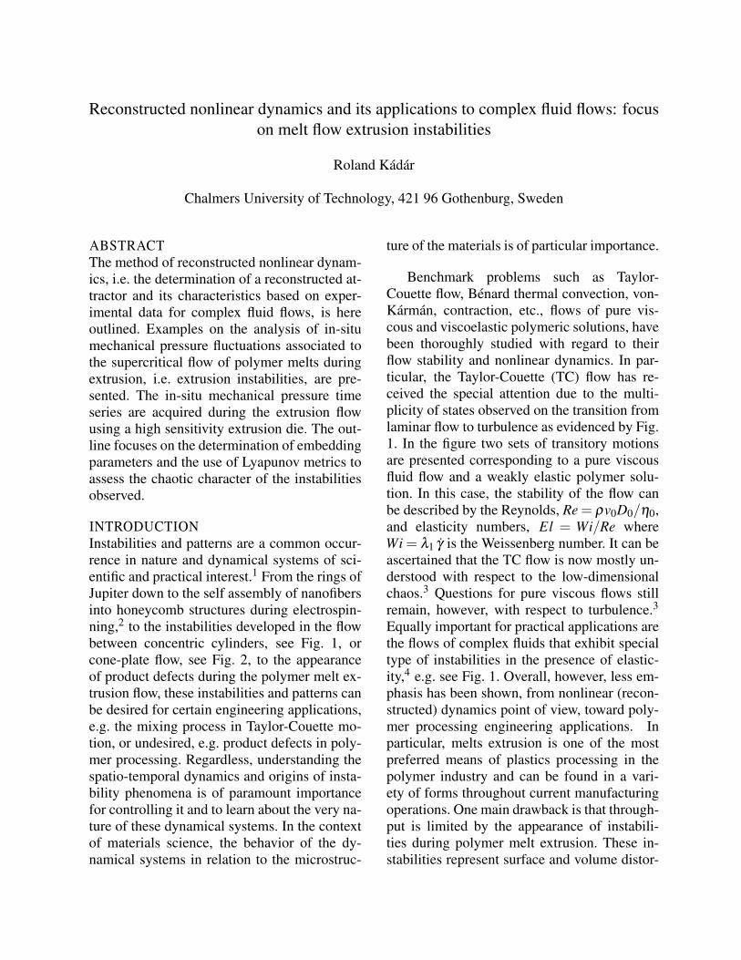
INTRODUCTIONInstabilities and patterns are a common occur-rence in nature and dynamical systems of sci-entific and practical interest.1 From the rings ofJupiter down to the self assembly of nanofibersinto honeycomb structures during electrospin-ning,2 to the instabilities developed in the flowbetween concentric cylinders, see Fig. 1, orcone-plate flow, see Fig. 2, to the appearanceof product defects during the polymer melt ex-trusion flow, these instabilities and patterns canbe desired for certain engineering applications,e.g. the mixing process in Taylor-Couette mo-tion, or undesired, e.g. product defects in poly-mer processing. Regardless, understanding thespatio-temporal dynamics and origins of insta-bility phenomena is of paramount importancefor controlling it and to learn about the very na-ture of these dynamical systems. In the contextof materials science, the behavior of the dy-namical systems in relation to the microstruc-

ture of the materials is of particular importance.

Benchmark problems such as Taylor-Couette flow, Bénard thermal convection, von-Kármán, contraction, etc., flows of pure vis-cous and viscoelastic polymeric solutions, havebeen thoroughly studied with regard to theirflow stability and nonlinear dynamics. In par-ticular, the Taylor-Couette (TC) flow has re-ceived the special attention due to the multi-plicity of states observed on the transition fromlaminar flow to turbulence as evidenced by Fig.1. In the figure two sets of transitory motionsare presented corresponding to a pure viscousfluid flow and a weakly elastic polymer solu-tion. In this case, the stability of the flow canbe described by the Reynolds, Re = ρv0D0/η0,and elasticity numbers, El = Wi/Re whereWi = λ1 γ̇ is the Weissenberg number. It can beascertained that the TC flow is now mostly un-derstood with respect to the low-dimensionalchaos.3 Questions for pure viscous flows stillremain, however, with respect to turbulence.3

Equally important for practical applications arethe flows of complex fluids that exhibit specialtype of instabilities in the presence of elastic-ity,4 e.g. see Fig. 1. Overall, however, less em-phasis has been shown, from nonlinear (recon-structed) dynamics point of view, toward poly-mer processing engineering applications. Inparticular, melts extrusion is one of the mostpreferred means of plastics processing in thepolymer industry and can be found in a vari-ety of forms throughout current manufacturingoperations. One main drawback is that through-put is limited by the appearance of instabili-ties during polymer melt extrusion. These in-stabilities represent surface and volume distor-

t

t

t

t

t

Re = 112

TVF

zTVFTVFTVFTVFTVFTVF

DODODODODODO

WVFWVFWVFWVFWVFWVF

WTVWTVWTVWTVWTVWTV

Re = 145, El = 0.47 Re = 800, El = 0

0.18

m

DO

DODODODODODODO

z

Re = 150, El = 0

TVFTVFTVFTVFTVFTVF

Re = 99, El = 0.47

Re = 117, El = 0.47

z

R

R1L

t

z

Δz

Re = 130, El = 0 t

t

t

t

t

zTVFTVFTVFTVFTVFTVF

DODODODODODO

WVFWVFWVFWVFWVFWVF

WTVWTVWTVWTVWTVWTV

Re = 145, El = 0.47 Re = 800, El = 0

DO

DODODODODODODO

z

Re = 150, El = 0

TVFTVFTVFTVFTVFTVF

Re = 99, El = 0.47

Re = 117, El = 0.47 t

z

Re = 130, El = 0

z

Figure 1. Examples of nonlinear phenomena in the flow between concentric cylinders, whereinner cylinder is rotating and the outer one is at rest, i.e. Taylor-Couette flow. The instability types

are represented as spatio-temporal diagrams and are: TVF - Taylor vortex flow, WVF - wavyvortex flow, TWV - turbulent wavy vortices and DO - disordered oscillations. The instabilities on

the left correspond to the case of a pure viscous fluid whereas those on the right for a weaklyelastic polyacrylamide solution.12, 13

tions of the extrudate that can significantly af-fect the mechanical performance and appear-ance of the final products.5 Comprehensive re-views on the subject of polymer processing in-stabilities can be found elsewhere.4, 6 With theadvent of high sensitivity in situ mechanicalpressure instability detection systems in poly-

RR

polymer solutionpolymer solutionpolymer solutionpolymer solutionpolymer solutionpolymer solution

airairairairairair

polymer solutionpolymer solutionpolymer solutionpolymer solutionpolymer solutionpolymer solution

airairairairairair

Figure 2. Nonlinear phenomena observed in atwo-phase viscoelastic cone-plate flow. Theexperiments were performed together with

Prof. C. Balan.

mer characterization/processing equipments,7

new means of scientific inquiry are opened. Inthis context, we provide a new perspective onthe extrusion flow instabilities by providing in-sight into their chaotic character through non-linear time series analysis. Some of the in-stability types investigated in the scientific lit-erature, for the extrusion of a linear low den-sity polyethylenes (LLDPE) and low densitypolyethylenes (LDPE), are presented in Fig. 3and Fig. 4 (polymer data can be found in aheadTable 1). With increasing control parameter, i.e.the apparent shear rate, γ̇ , the following extru-date states/patterns are distinguished based ontheir appearance: smooth extrudate, sharkskin,stick-slip, or spurt, and gross melt fracture forLLDPE, whereas in the case of LDPE follow-ing smooth extrudate flow instabilities differentfrom those of sharkskin instability appear, fol-lowed by a bifurcation to a secondary super-critical regime regime through the addition of a

Figure 3. Optical visualization of typical instabilities observed in the extrusion flow of linear/shortchain branched polyethylenes.

Figure 4. Optical visualization of typicalinstabilities observed in the extrusion flow of

long chain branched polyethylenes.

low frequency component.In this framework, the method of nonlinear

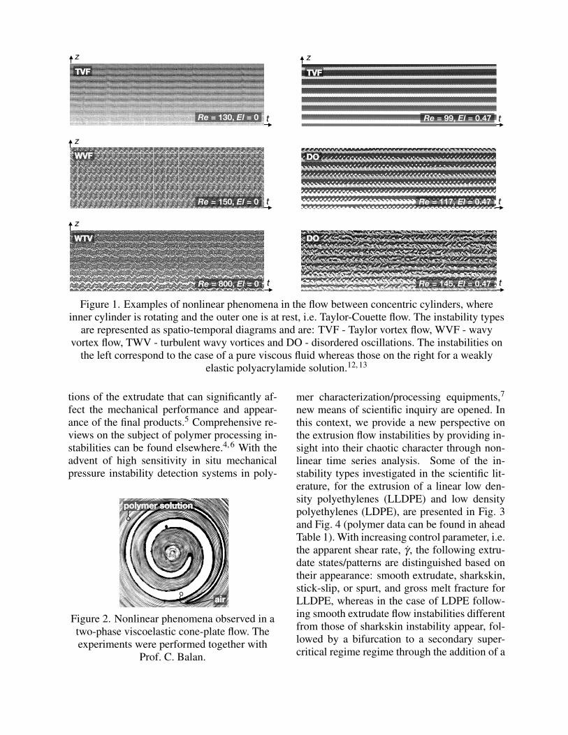
reconstructed dynamics is applied to the poly-mer melt extrusion stability problem, as an ap-proach to investigate the nature of the dynami-cal system of complex fluid flows. An overviewof the method is shown in Fig. 5. A typical ap-proach in nonlinear dynamics comprises of agiven set of equations whose complex solutionscomprise an attractor in the phase space. An’inverse’ approach is aimed at creating a recon-structed phase space from experimental timeseries, even without knowing the original gov-erning equations. In this approach, the recon-structed phase space is defined by some em-bedding parameters, i.e. delay time, τ , and anembedding dimension, dE . Various methods areavailable for the estimation of embedding pa-rameters.11 Fundamentally, the reconstructionis based on Takens’ embedding theorem,8 thatstates that the reconstructed phases space is a

mapping of the original phase space providedthat dE ≥ 2n+ 1, where n is the dimension ofthe original phase space. In other words, thedynamical system can be reconstructed fromexperimental time series generated by an un-known system of equations. Thus, in determin-istic manner, the state space reconstruction ofan unknown nonlinear function F from time se-ries can be represented as:

[x(t),x(t− τ),x(t−2τ), ...

x(t−dEτ)]→ F (1)

Thus, there exists a topological mapping be-tween the real and reconstructed phase spaces.The topological mapping can be quantified in anumber of ways, including by considering thedivergence of nearby trajectories, i.e. Lyapunovexponents, among others. The outlined frame-work can be used to further predict the sig-nal using e.g. artificial neural networks, F →x(t + τ).

EXPERIMENTALTwo samples of commercial polyethylene withdifferent molecular topologies were used ascase study. The first, a low density polyethylene(LDPE; Lupolen 1840 H), is characterized by arandom long-chained molecular structure. Thesecond sample is a linear low density polyethy-lene (LLDPE; Escorene LLN 1201 XV) thatdiffers from the LDPE through its linear molec-ular structure, molecular mass and its distri-bution. Their physical properties are listed inTable 1 whereas the rheological properties areshown in Fig. 6. The flow stability of the

G(t� τ)

Cauchy equilibrium eq.Constitutive relationBoundary conditions

Solution of the dynamical system

Attractor in Phase space

Experimental data Reconstructed attractor

Topological equivalence

Estimation of embedding parameters

dE � 2n + 1

τ, dE

Delay time Embedding dimension

F�(t)

F(t)

G(t)

Figure 5. Generic principle of nonlinear reconstructed dynamics.

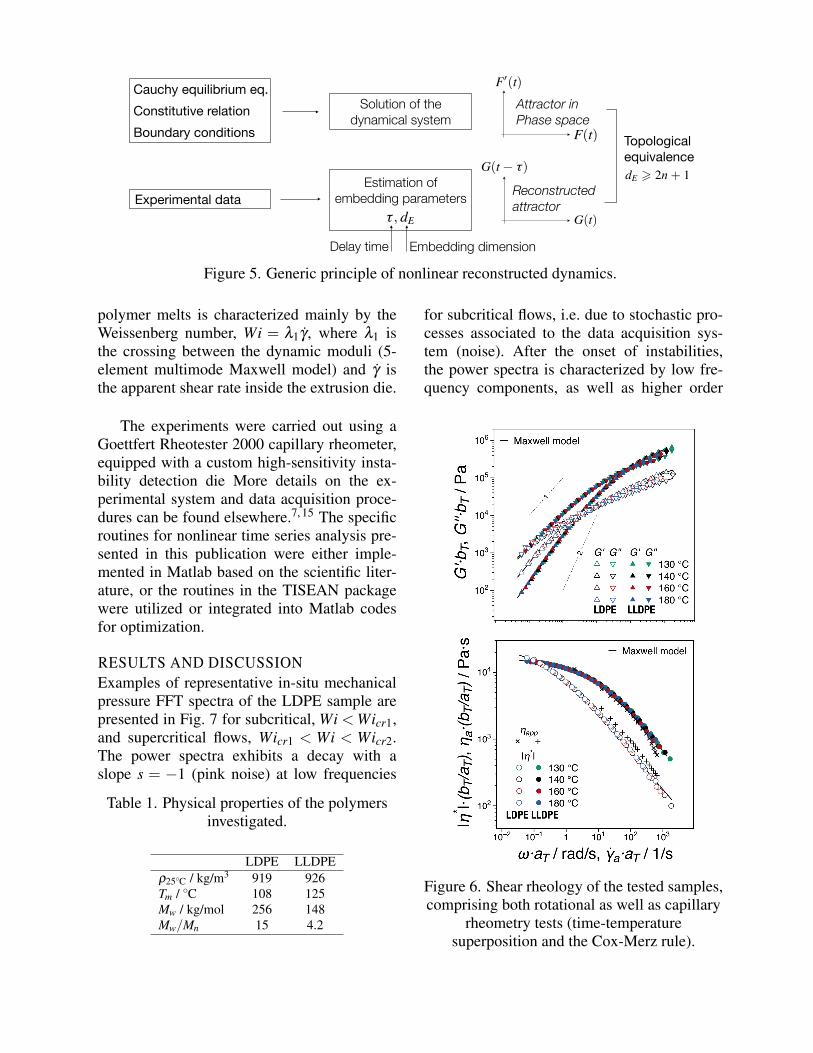
polymer melts is characterized mainly by theWeissenberg number, Wi = λ1γ̇ , where λ1 isthe crossing between the dynamic moduli (5-element multimode Maxwell model) and γ̇ isthe apparent shear rate inside the extrusion die.

The experiments were carried out using aGoettfert Rheotester 2000 capillary rheometer,equipped with a custom high-sensitivity insta-bility detection die More details on the ex-perimental system and data acquisition proce-dures can be found elsewhere.7, 15 The specificroutines for nonlinear time series analysis pre-sented in this publication were either imple-mented in Matlab based on the scientific liter-ature, or the routines in the TISEAN packagewere utilized or integrated into Matlab codesfor optimization.

RESULTS AND DISCUSSIONExamples of representative in-situ mechanicalpressure FFT spectra of the LDPE sample arepresented in Fig. 7 for subcritical, Wi < Wicr1,and supercritical flows, Wicr1 < Wi < Wicr2.The power spectra exhibits a decay with aslope s = −1 (pink noise) at low frequencies

Table 1. Physical properties of the polymersinvestigated.

LDPE LLDPEρ25◦C / kg/m3 919 926Tm / ◦C 108 125Mw / kg/mol 256 148Mw/Mn 15 4.2

for subcritical flows, i.e. due to stochastic pro-cesses associated to the data acquisition sys-tem (noise). After the onset of instabilities,the power spectra is characterized by low fre-quency components, as well as higher order

Figure 6. Shear rheology of the tested samples,comprising both rotational as well as capillary

rheometry tests (time-temperaturesuperposition and the Cox-Merz rule).

(a) (b)

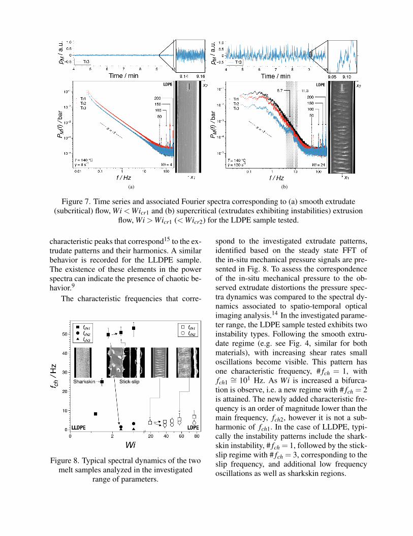
Figure 7. Time series and associated Fourier spectra corresponding to (a) smooth extrudate(subcritical) flow, Wi <Wicr1 and (b) supercritical (extrudates exhibiting instabilities) extrusion

flow, Wi >Wicr1 (<Wicr2) for the LDPE sample tested.

characteristic peaks that correspond15 to the ex-trudate patterns and their harmonics. A similarbehavior is recorded for the LLDPE sample.The existence of these elements in the powerspectra can indicate the presence of chaotic be-havior.9

The characteristic frequencies that corre-

Figure 8. Typical spectral dynamics of the twomelt samples analyzed in the investigated

range of parameters.

spond to the investigated extrudate patterns,identified based on the steady state FFT ofthe in-situ mechanical pressure signals are pre-sented in Fig. 8. To assess the correspondenceof the in-situ mechanical pressure to the ob-served extrudate distortions the pressure spec-tra dynamics was compared to the spectral dy-namics associated to spatio-temporal opticalimaging analysis.14 In the investigated parame-ter range, the LDPE sample tested exhibits twoinstability types. Following the smooth extru-date regime (e.g. see Fig. 4, similar for bothmaterials), with increasing shear rates smalloscillations become visible. This pattern hasone characteristic frequency, # fch = 1, withfch1∼= 101 Hz. As Wi is increased a bifurca-

tion is observe, i.e. a new regime with # fch = 2is attained. The newly added characteristic fre-quency is an order of magnitude lower than themain frequency, fch2, however it is not a sub-harmonic of fch1. In the case of LLDPE, typi-cally the instability patterns include the shark-skin instability, # fch = 1, followed by the stick-slip regime with # fch = 3, corresponding to theslip frequency, and additional low frequencyoscillations as well as sharkskin regions.

2 34 567

891011

12131415dE

Nv=2

f d E (τ

)

−30

−25

−20

−15

−10

−5

0

τ / Tch

0 0.1 0.2 0.3 0.4 0.5 0.6 0.7 0.8 0.9 1.0 1.1 1.2

LDPE 160℃, 99 1/s

2 34 567

891011

12131415dE

Nv=2

f d E (τ

)

−30

−25

−20

−15

−10

−5

0

τ / Tch

0 0.5 1.0

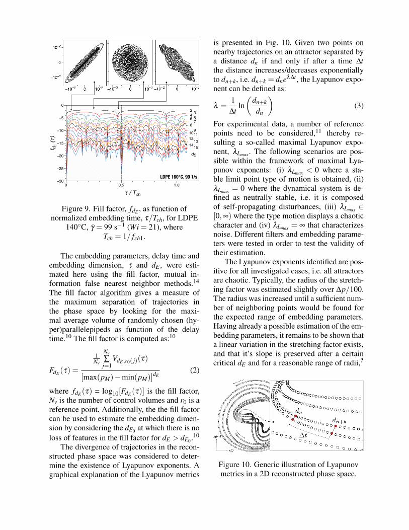
Figure 9. Fill factor, fdE , as function ofnormalized embedding time, τ/Tch, for LDPE

140◦C, γ̇ = 99 s−1 (Wi = 21), whereTch = 1/ fch1.

The embedding parameters, delay time andembedding dimension, τ and dE , were esti-mated here using the fill factor, mutual in-formation false nearest neighbor methods.14

The fill factor algorithm gives a measure ofthe maximum separation of trajectories inthe phase space by looking for the maxi-mal average volume of randomly chosen (hy-per)parallelepipeds as function of the delaytime.10 The fill factor is computed as:10

FdE (τ) =

1Nv

Nv

∑j=1

VdE ,r0( j)(τ)

[max(pM)−min(pM)]dE(2)

where fdE (τ) = log10[FdE (τ)] is the fill factor,Nv is the number of control volumes and r0 is areference point. Additionally, the the fill factorcan be used to estimate the embedding dimen-sion by considering the dE0 at which there is noloss of features in the fill factor for dE > dE0 .10

The divergence of trajectories in the recon-structed phase space was considered to deter-mine the existence of Lyapunov exponents. Agraphical explanation of the Lyapunov metrics

is presented in Fig. 10. Given two points onnearby trajectories on an attractor separated bya distance dn if and only if after a time ∆tthe distance increases/decreases exponentiallyto dn+k, i.e. dn+k = dneλ∆t , the Lyapunov expo-nent can be defined as:

λ =1∆t

ln(

dn+k

dn

)(3)

For experimental data, a number of referencepoints need to be considered,11 thereby re-sulting a so-called maximal Lyapunov expo-nent, λLmax . The following scenarios are pos-sible within the framework of maximal Lya-punov exponents: (i) λLmax < 0 where a sta-ble limit point type of motion is obtained, (ii)λLmax = 0 where the dynamical system is de-fined as neutrally stable, i.e. it is composedof self-propagating disturbances, (iii) λLmax ∈[0,∞) where the type motion displays a chaoticcharacter and (iv) λLmax = ∞ that characterizesnoise. Different filters and embedding parame-ters were tested in order to test the validity oftheir estimation.

The Lyapunov exponents identified are pos-itive for all investigated cases, i.e. all attractorsare chaotic. Typically, the radius of the stretch-ing factor was estimated slightly over ∆p/100.The radius was increased until a sufficient num-ber of neighboring points would be found forthe expected range of embedding parameters.Having already a possible estimation of the em-bedding parameters, it remains to be shown thata linear variation in the stretching factor exists,and that it’s slope is preserved after a certaincritical dE and for a reasonable range of radii,?

Figure 10. Generic illustration of Lyapunovmetrics in a 2D reconstructed phase space.

(a) (b)

Figure 11. Examples of stretching factor showing the influence of embedding dimension, dE andradius of the Kantz algorithm, r: (a) r = 4.3 ·10−4 ·∆pM and (b) r = 2 ·10−4 ·∆pM. The dotted

lines represent a linear approximation of the stretching factor for dE = 11. Examples for LLDPE,T = 140◦C, γ̇ = 131 s−1 (Wi = 2.4).

r in Eq. (4). To compute the largest Lyapunovexponent the Kantz algorithm was used.11 Inthe Kantz algorithm, the stretching factor ofnearby trajectories is determined as11

S =1Nr

Nr

∑n0=1

ln

(1|uxn0|∑ ||dxn0−xn ||

)(4)

where Nr is the number of reference points,|uxn0| are the neighborhood points within a

cloud of radius r relative to the neighborhoodpoints and ||dxn0−xn|| is the Euclidean norm ofneighborhood points to the reference point.

Examples of representative stretching fac-tors are shown in Fig. 11, data computed usinga constant radius over the embedding dimen-sion range. In both cases, at the maximal dE in-vestigated, the total number of points with suf-ficient lump neighbors within the radius r ex-ceeds 2000 data points. The number of refer-ence points used was Nre f = 50,000. Thus, fordE > 8 there is little change in the linear slopeof the stretching factor. Overall, a linear diver-gence was found typically in the range of dE ∈[8,15] in accordance with the qualitative obser-vations deduced from computing the fractionof false nearest neighbors. The complete setof determined slopes of stretching factors’ lin-ear divergence is presented in Fig. 12. Overall,

there is good agreement between the dynamicalbehavior of λLmax and the in situ spectral andspatio-temporal dynamics observed, i.e. λLmax

is sensitive to the change of extrudate patterns.

SUMMARY AND CONCLUSIONSFor both polymer melt molecular architec-tures investigated new patterns result from thegrowth of low frequencies in addition to themain characteristic pattern frequency, whethersuperimposed or intermittently. In the frame-work of reconstructed dynamics, embeddingparameters were determined based on mainlyby considering a maximal separation of trajec-tories in a delayed representation. In the sub-sequent reconstructed phase spaces, the poly-mer melt instabilities investigated obeyed anexponential growth of trajectories in the re-constructed phase space for the recorded ex-trusion melt flow instabilities, i.e. there existsdE > dE0 for which a constant linear increasein the stretching factor is recorded, i.e. positivemaximal Lyapunov exponents.

ACKNOWLEDGEMENTSThe author is grateful to the financial supportof the CNCSIS BG Grant code 349, the DAADand DFG Grant WI 1911/14-1 for the differ-

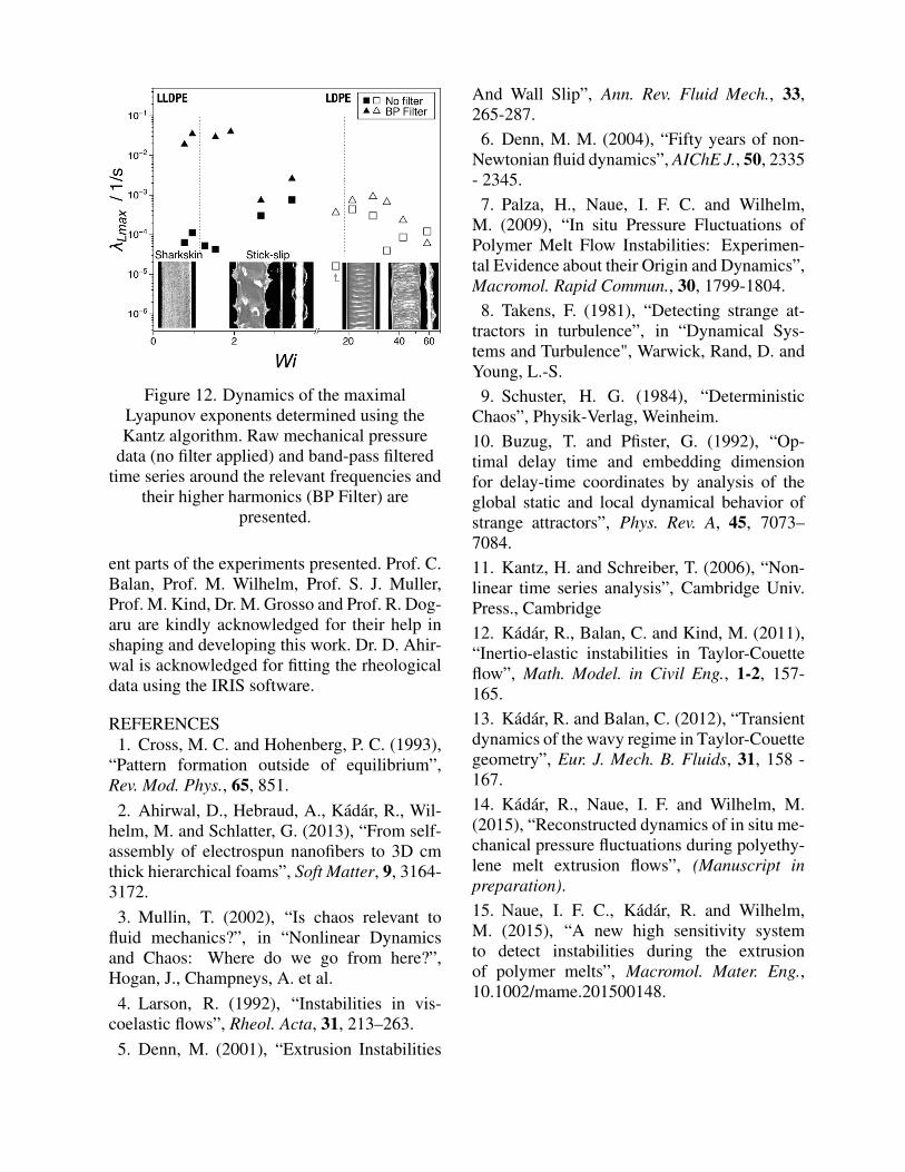
Figure 12. Dynamics of the maximalLyapunov exponents determined using theKantz algorithm. Raw mechanical pressure

data (no filter applied) and band-pass filteredtime series around the relevant frequencies and

their higher harmonics (BP Filter) arepresented.

ent parts of the experiments presented. Prof. C.Balan, Prof. M. Wilhelm, Prof. S. J. Muller,Prof. M. Kind, Dr. M. Grosso and Prof. R. Dog-aru are kindly acknowledged for their help inshaping and developing this work. Dr. D. Ahir-wal is acknowledged for fitting the rheologicaldata using the IRIS software.

REFERENCES1. Cross, M. C. and Hohenberg, P. C. (1993),

“Pattern formation outside of equilibrium”,Rev. Mod. Phys., 65, 851.2. Ahirwal, D., Hebraud, A., Kádár, R., Wil-

helm, M. and Schlatter, G. (2013), “From self-assembly of electrospun nanofibers to 3D cmthick hierarchical foams”, Soft Matter, 9, 3164-3172.3. Mullin, T. (2002), “Is chaos relevant to

fluid mechanics?”, in “Nonlinear Dynamicsand Chaos: Where do we go from here?”,Hogan, J., Champneys, A. et al.4. Larson, R. (1992), “Instabilities in vis-

coelastic flows”, Rheol. Acta, 31, 213–263.5. Denn, M. (2001), “Extrusion Instabilities

And Wall Slip”, Ann. Rev. Fluid Mech., 33,265-287.6. Denn, M. M. (2004), “Fifty years of non-

Newtonian fluid dynamics”, AIChE J., 50, 2335- 2345.7. Palza, H., Naue, I. F. C. and Wilhelm,

M. (2009), “In situ Pressure Fluctuations ofPolymer Melt Flow Instabilities: Experimen-tal Evidence about their Origin and Dynamics”,Macromol. Rapid Commun., 30, 1799-1804.8. Takens, F. (1981), “Detecting strange at-

tractors in turbulence”, in “Dynamical Sys-tems and Turbulence", Warwick, Rand, D. andYoung, L.-S.9. Schuster, H. G. (1984), “Deterministic

Chaos”, Physik-Verlag, Weinheim.10. Buzug, T. and Pfister, G. (1992), “Op-timal delay time and embedding dimensionfor delay-time coordinates by analysis of theglobal static and local dynamical behavior ofstrange attractors”, Phys. Rev. A, 45, 7073–7084.11. Kantz, H. and Schreiber, T. (2006), “Non-linear time series analysis”, Cambridge Univ.Press., Cambridge12. Kádár, R., Balan, C. and Kind, M. (2011),“Inertio-elastic instabilities in Taylor-Couetteflow”, Math. Model. in Civil Eng., 1-2, 157-165.13. Kádár, R. and Balan, C. (2012), “Transientdynamics of the wavy regime in Taylor-Couettegeometry”, Eur. J. Mech. B. Fluids, 31, 158 -167.14. Kádár, R., Naue, I. F. and Wilhelm, M.(2015), “Reconstructed dynamics of in situ me-chanical pressure fluctuations during polyethy-lene melt extrusion flows”, (Manuscript inpreparation).15. Naue, I. F. C., Kádár, R. and Wilhelm,M. (2015), “A new high sensitivity systemto detect instabilities during the extrusionof polymer melts”, Macromol. Mater. Eng.,10.1002/mame.201500148.