THESIS FOR THE DEGREE OF LICENTIATE OF ENGINEERING

Design of a fault-tolerant fractional slot PMSMfor a vehicle application

CHRISTIAN DU-BAR

Division of Electric Power Engineering

Department of Energy and Environment

CHALMERS UNIVERSITY OF TECHNOLOGY

Göteborg, Sweden 2015

Design of a fault-tolerant fractional slot PMSM

for a vehicle application

Christian Du-Bar

© Christian Du-Bar, 2015.

except where otherwise stated.

All rights reserved

Department of Energy and Environment

CHALMERS UNIVERSITY OF TECHNOLOGY

SE-412 96 Göteborg

Sweden

Telephone + 46 (0)31 772 00 00

Abstract

In automotive applications, the PMSM is an interesting alternative due to the

high efficiency requirement; as only a limited amount of energy can be stored

in the relatively expensive battery. Another advantage is the high torque and

power density since it is very important to save especially space but also weight

in vehicle applications. As the battery technology develops, pure electric cars

are expected to become a more and more interesting alternative. In case of pure

electric vehicles, it is natural that the requirement of reliability on the electric

drive system becomes an aspect of utmost importance as the electric drive is

the only driving force.

In this thesis a three phase fractional slot PMSM is designed and its possibility

to operate and to deliver an acceptable quality of performance even after a fault

occurs is investigated. The faults investigated are phase open circuit and phase

short circuit, and it is shown that the thesis machine design can be operated dur-

ing both circumstances. During normal operation, the fault-tolerant machine

design shows a similar performance as an existing design of the same size, where

fault-tolerance was not considered in the design. During fault, the maximum

torque is reduced by approximately 50 % and the maximum speed is reduced to

roughly 1/3 or 1/4 of the maximum speed in case of a phase open circuit fault

or a phase short circuit fault respectively. A semi-analytical machine modeling

approach are used to model the individual saturation levels of the phases suc-

cessfully. The same model is used to calculate new current waveforms that are

used to reduce the torque ripple during the unbalanced conditions associated

with the operation during fault. Further, a design procedure considering the

machine design performance in relation to its expected material cost is used

and presented.

iii

Keywords

Permanent magnet synchronous machine (PMSM), Fractional slot, Concentrated

windings, Fault-tolerance, Unbalanced operation, Saturation, Efficiency.

iv

Acknowledgements

The financial support from the Swedish innovation agency Vinnova via the for-

mer xEVCO project including Volvo Cars and SP, which this PhD project was a

part of, is gratefully appreciated.

I would like to thank my main supervisor and examiner Torbjörn Thiringer for

his great support and always very quick response with input and feedback. I

would of course also like to address special thanks to my supervisors Sonja Lund-

mark and Mikael Alatalo for their support and valuable input and comments.

Through all three of you in a combination, I think the quality of my work really

has been increased an extra level or two.

I would also like to thank all my colleagues, room-mates and friends at the Divi-

sion of Electric Power Engineering for creating such a nice and fun environment

to work in. Thanks also to the people one stair down at the Division of High Volt-

age Engineering, they also contribute to the appreciated working environment.

Finally, I would like to thank my family including my wonderful fiancée Gabriela

for endless love and support over the years.

Christian Du-Bar

Göteborg, November 2014

v

vi

Contents

Abstract iii

Acknowledgements v

Introduction 1

1 Machine Design Modeling 5

1.1 Electric and magnetic loading . . . . . . . . . . . . . . . . . . . . . . . . . . . 5

1.2 Permanent magnet flux . . . . . . . . . . . . . . . . . . . . . . . . . . . . . . . . 7

1.3 Core loss and core geometry . . . . . . . . . . . . . . . . . . . . . . . . . . . . 8

1.4 Thermal conductivity of the winding mix . . . . . . . . . . . . . . . . . . . 10

1.5 Pole and slot combinations . . . . . . . . . . . . . . . . . . . . . . . . . . . . . 12

1.6 Winding factor . . . . . . . . . . . . . . . . . . . . . . . . . . . . . . . . . . . . . . 13

1.7 MMF time and space harmonics . . . . . . . . . . . . . . . . . . . . . . . . . 15

1.8 Inductance calculation . . . . . . . . . . . . . . . . . . . . . . . . . . . . . . . . 19

2 Dynamic Modeling of PMSMs 23

2.1 Basic 3ph-model . . . . . . . . . . . . . . . . . . . . . . . . . . . . . . . . . . . . . 23

2.2 Flux model in the rotating dq-reference frame . . . . . . . . . . . . . . . 25

2.3 Basic modeling of chosen faults . . . . . . . . . . . . . . . . . . . . . . . . . . 26

2.3.1 Phase short circuit . . . . . . . . . . . . . . . . . . . . . . . . . . . . . . 27

2.3.2 Phase open circuit . . . . . . . . . . . . . . . . . . . . . . . . . . . . . . 27

2.4 Control . . . . . . . . . . . . . . . . . . . . . . . . . . . . . . . . . . . . . . . . . . . 29

2.4.1 Ordinary PI controller . . . . . . . . . . . . . . . . . . . . . . . . . . . 29

2.4.2 Resonant and PI controller . . . . . . . . . . . . . . . . . . . . . . . . 29

2.5 Converter limitations . . . . . . . . . . . . . . . . . . . . . . . . . . . . . . . . . 30

3 Design of fault-tolerant fractional slot machines 35

3.1 Design specification . . . . . . . . . . . . . . . . . . . . . . . . . . . . . . . . . . 35

3.1.1 Rating of the reference machine . . . . . . . . . . . . . . . . . . . . 36

3.2 Selection of pole and slot combination . . . . . . . . . . . . . . . . . . . . 38

3.3 FEA and material data . . . . . . . . . . . . . . . . . . . . . . . . . . . . . . . . . 43

vii

3.3.1 Finite Element Analysis . . . . . . . . . . . . . . . . . . . . . . . . . . 43

3.3.2 Material data . . . . . . . . . . . . . . . . . . . . . . . . . . . . . . . . . . 43

3.4 Design strategy . . . . . . . . . . . . . . . . . . . . . . . . . . . . . . . . . . . . . . 44

3.4.1 Design variables . . . . . . . . . . . . . . . . . . . . . . . . . . . . . . . . 44

3.4.2 Design variable combinations . . . . . . . . . . . . . . . . . . . . . . 46

3.4.3 From design variables to geometry parameters . . . . . . . . . 46

4 Analysis of fault-tolerant fractional slot machine designs 49

4.1 Machine design selection . . . . . . . . . . . . . . . . . . . . . . . . . . . . . . 49

4.1.1 Estimation of the current material costs . . . . . . . . . . . . . . 49

4.1.2 Torque per cost for different cost scenarios . . . . . . . . . . . . 51

4.1.3 Cost efficiency of the 12/5 machine designs . . . . . . . . . . . . 53

4.1.4 Cost efficiency of the 24/11 machine designs . . . . . . . . . . . 57

4.1.5 Torque speed characteristics of the 12/5 machine designs . 61

4.1.6 Torque speed characteristics of the 24/11 machine designs 62

4.2 The two selected machine designs . . . . . . . . . . . . . . . . . . . . . . . . 63

4.2.1 Estimation of end-windings . . . . . . . . . . . . . . . . . . . . . . . 63

4.2.2 Turn selection . . . . . . . . . . . . . . . . . . . . . . . . . . . . . . . . . 65

4.2.3 Thermal impact of the slot geometry . . . . . . . . . . . . . . . . . 66

4.2.4 Thermal restriction of the electric loading . . . . . . . . . . . . . 68

4.3 Efficiency . . . . . . . . . . . . . . . . . . . . . . . . . . . . . . . . . . . . . . . . . . 70

4.4 Summary of comparison . . . . . . . . . . . . . . . . . . . . . . . . . . . . . . . 74

5 Per phase flux machine model 75

5.1 Flux representation in a single phase . . . . . . . . . . . . . . . . . . . . . . 75

5.1.1 Per phase flux and torque maps . . . . . . . . . . . . . . . . . . . . 77

5.2 Numerical solution of 2-phase MTPA operation . . . . . . . . . . . . . . 81

6 Further analysis of one fault-tolerant fractional slot machine design 83

6.1 Unbalanced operation using resonant controller . . . . . . . . . . . . . 84

6.1.1 Phase open circuit . . . . . . . . . . . . . . . . . . . . . . . . . . . . . . 84

6.1.2 Phase short circuit . . . . . . . . . . . . . . . . . . . . . . . . . . . . . . 89

6.2 Numerically calculated unbalanced operating points . . . . . . . . . . 92

6.2.1 Filtering of numerically calculated currents . . . . . . . . . . . . 92

6.2.2 Torque speed characteristics . . . . . . . . . . . . . . . . . . . . . . . 93

6.2.3 Efficiency . . . . . . . . . . . . . . . . . . . . . . . . . . . . . . . . . . . . . 95

6.3 2D modeling of MMF harmonic content and

losses on the rotor side . . . . . . . . . . . . . . . . . . . . . . . . . . . . . . . . 97

7 Conclusions and future work 101

7.1 Conclusions . . . . . . . . . . . . . . . . . . . . . . . . . . . . . . . . . . . . . . . . 101

7.2 Future Work . . . . . . . . . . . . . . . . . . . . . . . . . . . . . . . . . . . . . . . . 103

viii

Introduction

Background

Permanent magnet synchronous machines (PMSM) of different sizes are used in

a great number of applications. They are often competitive in the low power re-

gion due to high efficiency, and in the medium power region due to high torque

and power density. At higher power levels, PMSM are sometimes used as wind

power generators, also offering the possibility to remove the gear box and op-

erate in a direct-drive configuration. The PMSM are often categorized depend-

ing on the permanent magnet (PM) and rotor configuration as well as the flux

path and air-gap arrangement. The PM can be surface-mounted or interior-

mounted and the same stator can be used for both types of machines. Further,

the PMSM can be divided into radial flux machines where the magnetic flux is

crossing the air-gap in the radial direction and axial flux machines where the

magnetic flux crosses the air-gap in the axial direction. Again, it is often possi-

ble to utilize the same pole, slot and winding configuration. A third group is the

transverse flux machines, that benefit from the involvement of a more compli-

cated magnetic circuit in favor of a simpler electrical circuit.

In automotive applications, the PMSM is an interesting alternative due to the

high efficiency requirement; as only a limited amount of energy can be stored

in the relatively expensive battery. Another advantage is the high torque and

power density since it is very important to save especially space but also weight

in vehicle applications. The introduction of electric drives into vehicles may

improve the fuel economy and reduce the environmental emissions but allows

also for new features such as increased safety and passenger comfort. As the

battery technology develops, pure electric cars are expected to become a more

and more interesting alternative. In case of pure electric vehicles, it is natu-

ral that the requirement of reliability on the electric drive system becomes a

more important aspect as the electric drive is the only driving force. Accord-

ing to [1], the trend towards autonomic control systems increases the interest of

fault-tolerant capability in automotive applications. It is therefore of interest to

combine the advantages of high efficiency, torque and power density associated

1

with PMSM and the ability of operation during isolated failures in the machine

or the converter. In [2], it is stated that the introduction of fault-tolerance into

the permanent magnet machine design is related with only a modest reduction

of the torque capability.

Fault-tolerant electric machines

There are two possible meanings of fault-tolerant electric drive systems [3]:

• a system designed to reduce the number of fault occurrences.

• a system that is able to operate even after a fault occurs, on short-term or

continuously.

where the second group can be divided into two subgroups

- a PM motor drive configuration with independent phases, that may

operate independently. In case of a fault in one phase, the other

phases can still be operated.

- a redundant system, where the number of one or more components

is extended. During healthy operation, the redundant components

are totally or partially excluded.

From a practical point of view, it is not that straightforward to distinguish be-

tween a system or a machine that is designed to reduce the number of fault oc-

currences or is designed to be able to operate even after a fault occurs. In the

case of a machine design with independent phases in order to better operate

after a fault occurs, a low mutual coupling is suggested in [2] and [3]. However,

the electrical insulation between phases may be increased as a consequence.

An increased electrical phase separation is also mentioned in [3], both to limit

the probability of fault occurrence, and as well to mitigate a fault propagation to

other motor parts. Multiphase systems (a phase number greater than three) is a

common approach when designing fault tolerant drive systems, considered in

[2] and [4] for instance. The relative torque or power loss when one phase is lost,

is in this way of course decreased, but to the cost of an increased complexity of

the system. A fault-tolerant multiphase system could beneficially be designed

with independent phases to be able to operate when a fault occurs, but can also

be considered as a redundant system as the number of components (the phases)

is increased.

From a machine design point of view, the fractional slot type of PMSM with con-

centrated windings has been considered as a promising alternative to achieve

an independence between phases and to allow for operation during failures in a

2

single phase. In [5], a summary of the opportunities and challenges of the frac-

tional slot concentrated winding PMSM can be found; some of the advantages

that are mentioned are high power density, efficiency and fault-tolerance. One

of the key challenges that are raised is the reduction of rotor losses since these

tend to be high in fractional slot machines. Methods to reduce the rotor losses

are investigated by [6], and in [7] substantial reductions of both rotor iron and

permanent magnet losses are shown. The concept of fractional slot PMSM with

concentrated windings are used when designing fault-tolerant multiphase ma-

chines in both [8] and [3]. The basic rules of fault-tolerant machine design are

well described in [2]. The electrical, magnetic and thermal insulation between

phases are important properties as well as limitation of the short circuit current.

The unbalanced conditions, associated with the operation during fault, impose

additional requirements on both the controller and the converter. The control

of electric machines, mainly during phase open circuit fault, has been investi-

gated extensively in the literature. In [9] and [10], similar control methods uti-

lizing resonant controllers are proposed but different converter topologies are

considered. Two alternative control methods are suggested in [11], where feed

forward terms are used to compensate for the unbalanced condition. In addi-

tion, a number of faults that occur in a PMSM drive system under field weaken-

ing operation are investigated in [12]. However, most studies are focused on the

control perspective and rather simple machine models are used, often suppos-

ing a magnetic linearity. Regarding the theme of handling individual saturation

levels in the different phases, there seem to be a lack of literature, according to

the author’s knowledge.

3

Purpose and main contribution of the thesis

The aim of this thesis is to design a three phase fractional slot PMSM and eval-

uate the possibility to operate and to deliver an acceptable quality of perfor-

mance even after a fault occurs. Another part is to compare the fault-tolerant

design with an existing design, where fault-tolerance was not considered in the

design. The machine is to be designed fault-tolerant with a low mutual coupling

between the phases and the electrical faults that are to be considered are phase

open circuit fault and phase short circuit fault. This thesis is focused on the ma-

chine design perspective, not supposing a magnetic linearity, and the control

and converter topologies are treated briefly only.

Some of the contributions by this licentiate thesis work can be listed as

• Development and demonstration of a machine design procedure where

the relation between machine performance and material cost is consid-

ered.

• Introduction of a machine modeling technique that utilizes the weak mag-

netic coupling between the phases of a fault-tolerant PMSM, in order to

model the unbalanced saturation associated with operation during fault

more accurately.

• Quantification of the torque speed characteristics and efficiency when

one PMSM is operated during phase open circuit fault or phase short cir-

cuit fault.

4

Chapter 1

Machine Design Modeling

This chapter provides some basic machine modeling theory from a machine

design perspective. The theory is described on the basis that it is a three phase

fractional slot PMSM with surface mounted permanent magnets and concen-

trated double-layer windings that is to be designed. However, it is possible to

adapt most of the modeling techniques presented in this chapter to design of

other types of machines as well.

1.1 Electric and magnetic loading

In a PMSM with surface mounted permanent magnets, where the inductance

is independent of the rotor position, the torque is determined by the flux from

the permanent magnets, Ψm , and the flux induced by the stator, Ψi nd = Li , il-

lustrated in Figure 1.1.δ

Ψm

Ψi nd

Figure 1.1: Illustration of how torque is produced between two magnetic fields.

5

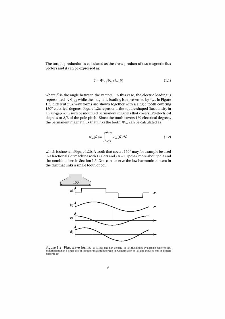
The torque production is calculated as the cross-product of two magnetic flux

vectors and it can be expressed as,

T =Ψi ndΨm s i n (δ) (1.1)

where δ is the angle between the vectors. In this case, the electric loading is

represented by Ψi nd while the magnetic loading is represented by Ψm . In Figure

1.2, different flux waveforms are shown together with a single tooth covering

150o electrical degrees. Figure 1.2a represents the square shaped flux density in

an air-gap with surface mounted permanent magnets that covers 120 electrical

degrees or 2/3 of the pole pitch. Since the tooth covers 150 electrical degrees,

the permanent magnet flux that links the tooth, Ψm , can be calculated as

Ψm (θ ) =

∫ θ+75

θ−75

Bm (θ )dθ (1.2)

which is shown in Figure 1.2b. A tooth that covers 150o may for example be used

in a fractional slot machine with 12 slots and 2p = 10 poles, more about pole and

slot combinations in Section 1.5. One can observe the low harmonic content in

the flux that links a single tooth or coil.

150o

a)

b)

c)

d)

Figure 1.2: Flux wave forms; a) PM air-gap flux density. b) PM flux linked by a single coil or tooth.c) Induced flux in a single coil or tooth for maximum torque. d) Combination of PM and induced flux in a singlecoil or tooth

6

In order to maximize the torque in (1.1), the angle, δ, between the induced flux,

Ψi nd , and the permanent magnet flux, Ψm , should be 90o . The induced flux,

leading the permanent magnet flux by 90o , is illustrated in Figure 1.2c. The total

flux in the tooth is the sum of the permanent magnet flux and the induced flux,

Ψt o o t h (θ ) =Ψi nd (θ ) +Ψm (θ ) = Li (θ ) +Ψm (θ ) (1.3)

which is shown in Figure1.2d. It should be noticed that the tooth carries a mix

of permanent magnet flux and induced flux, although the angle between the

permanent magnet flux and the current is 90o . By studying Figure 1.2 b and

c, one can observe that the tooth carries a mix of the two fluxes at all angles

except when one of the fluxes is crossing zero. As only one tooth is studied at

the moment, one flux has its peak when the other one is zero. This is not true

when the coils of several teeth are connected together and if the distribution

factor is not ideal, kd 6= 1. The distribution factor will be introduced later in

Section 1.6. From a design point of view, this implies that flux paths must be

designed with respect to the combination of permanent magnet and induced

flux levels. It is also clear that any orthogonal flux vectors appearing in a phasor

diagram are not independent, as they share the same non-linear iron flux paths.

1.2 Permanent magnet flux

As a simple approach, the magnetic flux distribution from a surface mounted

permanent magnet can be considered as square shaped with an amplitude Bm ,

illustrated in Figure 1.3.

Bm B1

Figure 1.3: Permanent magnet air-gap flux density waveforms.

If the permanent magnets covers 120 electrical degrees or 2/3 of the pole pitch,

the peak value of the fundamental, B1, can be calculated as,

7

B1 =4p

3

2πBm (1.4)

A permanent magnet that covers 2/3 of the pole pitch is often considered a suit-

able choice, due to the utilization of the permanent magnet flux and to achieve

a low cogging torque. If the reluctance of the iron paths and the leakage flux are

neglected, the required length of the permanent magnets, lp m , is expressed as

lp m =µlg

Br

Bm−1

(1.5)

where lg is the air-gap length, µ the relative permability of the permanent mag-

nets and Br is the residual flux density of the permanent magnets.

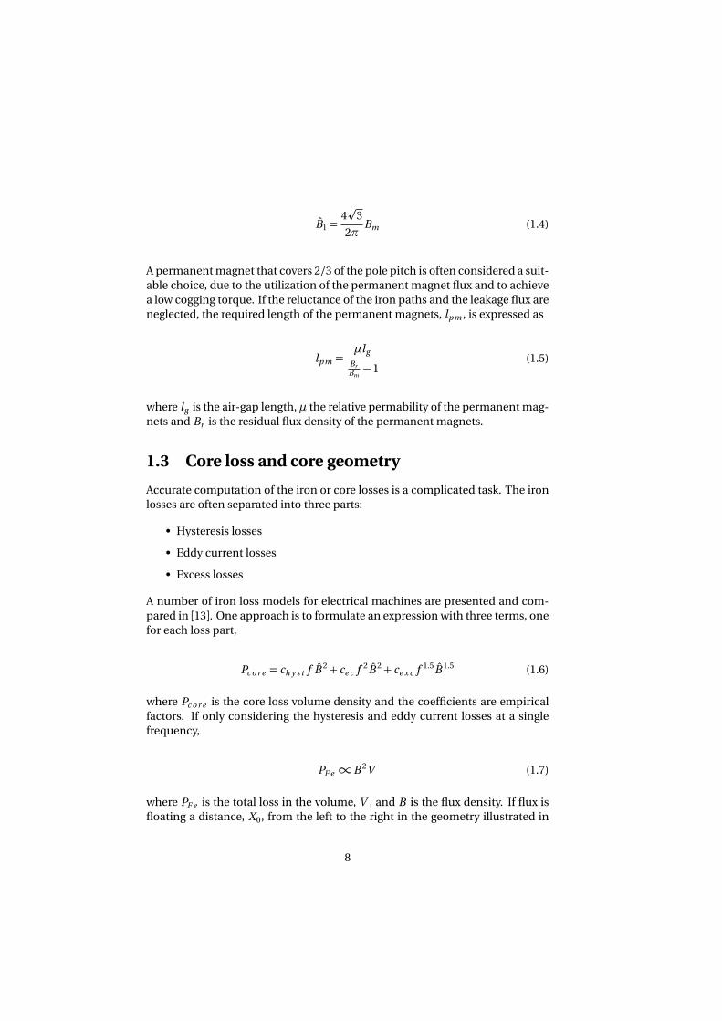
1.3 Core loss and core geometry

Accurate computation of the iron or core losses is a complicated task. The iron

losses are often separated into three parts:

• Hysteresis losses

• Eddy current losses

• Excess losses

A number of iron loss models for electrical machines are presented and com-

pared in [13]. One approach is to formulate an expression with three terms, one

for each loss part,

Pc o r e = ch y s t f B 2+ ce c f 2B 2+ ce x c f 1.5B 1.5 (1.6)

where Pc o r e is the core loss volume density and the coefficients are empirical

factors. If only considering the hysteresis and eddy current losses at a single

frequency,

PF e ∝ B 2V (1.7)

where PF e is the total loss in the volume, V , and B is the flux density. If flux is

floating a distance, X0, from the left to the right in the geometry illustrated in

8

Figure 1.4 and the flux is assumed to be uniformed distributed along a vertical

segment,

B =φ

A(1.8)

whereφ is the total flux that crosses each segment and A is the one-dimensional

area of a segment in vertical direction.

Y0

X0

∆Y0

∆Y0

Figure 1.4: Illustration of a segmented flux path volume.

The volume of a single element, V , is the horizontal thickness of a segment, l ,

multiplied by the one-dimensional area, A. Then, (1.7) and (1.8) together gives,

PF e ∝1

A2l A =

l

A(1.9)

which implies that the reluctance,ℜ, of the path X0, when carrying the total flux

φ, should be minimized in order to minimize the core loss since,

ℜ= l

µA(1.10)

For a flux path of the length X0 and the constant core volume V = X0 · Y0, the

variable ∆Y0 is used to vary the shape of the geometry. The reluctance, when

dividing the flux path into k segments, can be expressed as

ℜ= 1

µ

k∑

n=1

X0

k (Y0−∆Y0) +2∆Y0n(1.11)

9

The reluctance in (1.11) has a minimum for ∆Y0 = 0, corresponding to a con-

stant cross-sectional area along the flux path and evenly distributed flux.

The reasoning in this section together with knowledge about how the flux is di-

vided between different paths can be applied when dimensioning the flux paths.

It is beneficial to aim for constant flux densities along flux paths.

1.4 Thermal conductivity of the winding mix

When modeling the thermal characteristics of the windings, the copper conduc-

tors and the impregnation material between the conductors are often treated

as a mix material with an equivalent thermal conductivity. As the thermal con-

ductivity of copper is much higher than for the impregnation material, 1:1833 in

[14], both the conductivity of the impregnation material and the distribution of

the copper wires are of great importance when determining an equivalent ther-

mal conductivity of the material mix. Conductors of the same size placed in a

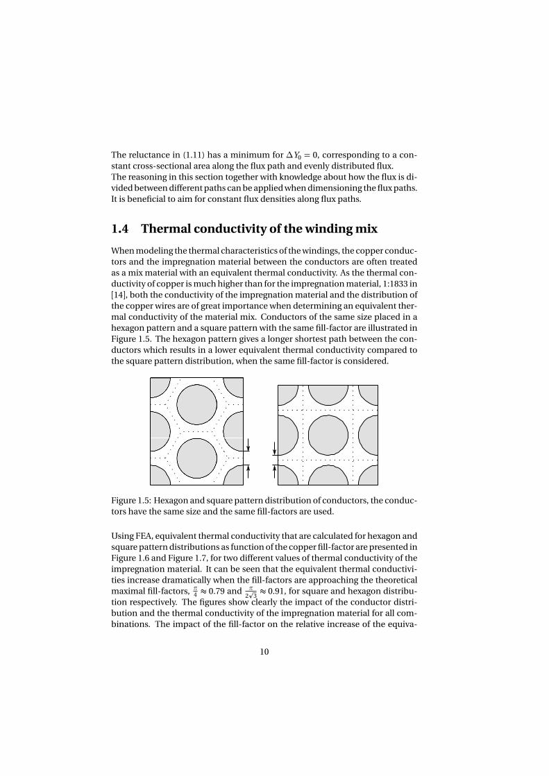
hexagon pattern and a square pattern with the same fill-factor are illustrated in

Figure 1.5. The hexagon pattern gives a longer shortest path between the con-

ductors which results in a lower equivalent thermal conductivity compared to

the square pattern distribution, when the same fill-factor is considered.

Figure 1.5: Hexagon and square pattern distribution of conductors, the conduc-

tors have the same size and the same fill-factors are used.

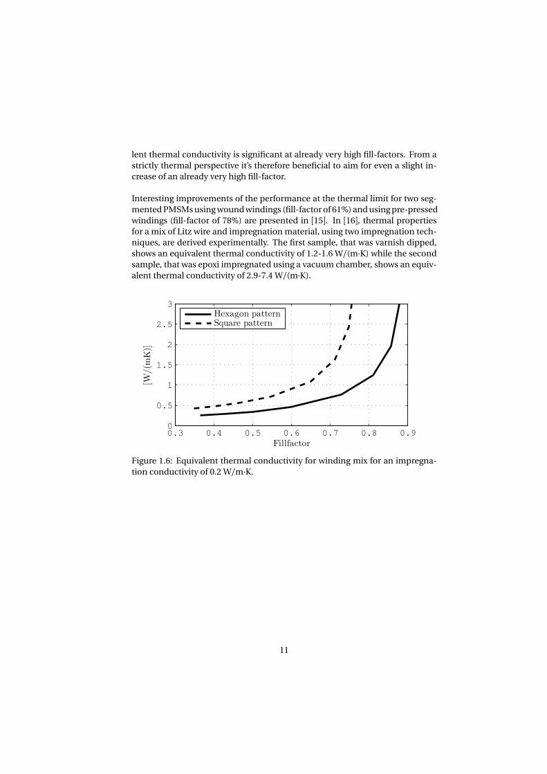
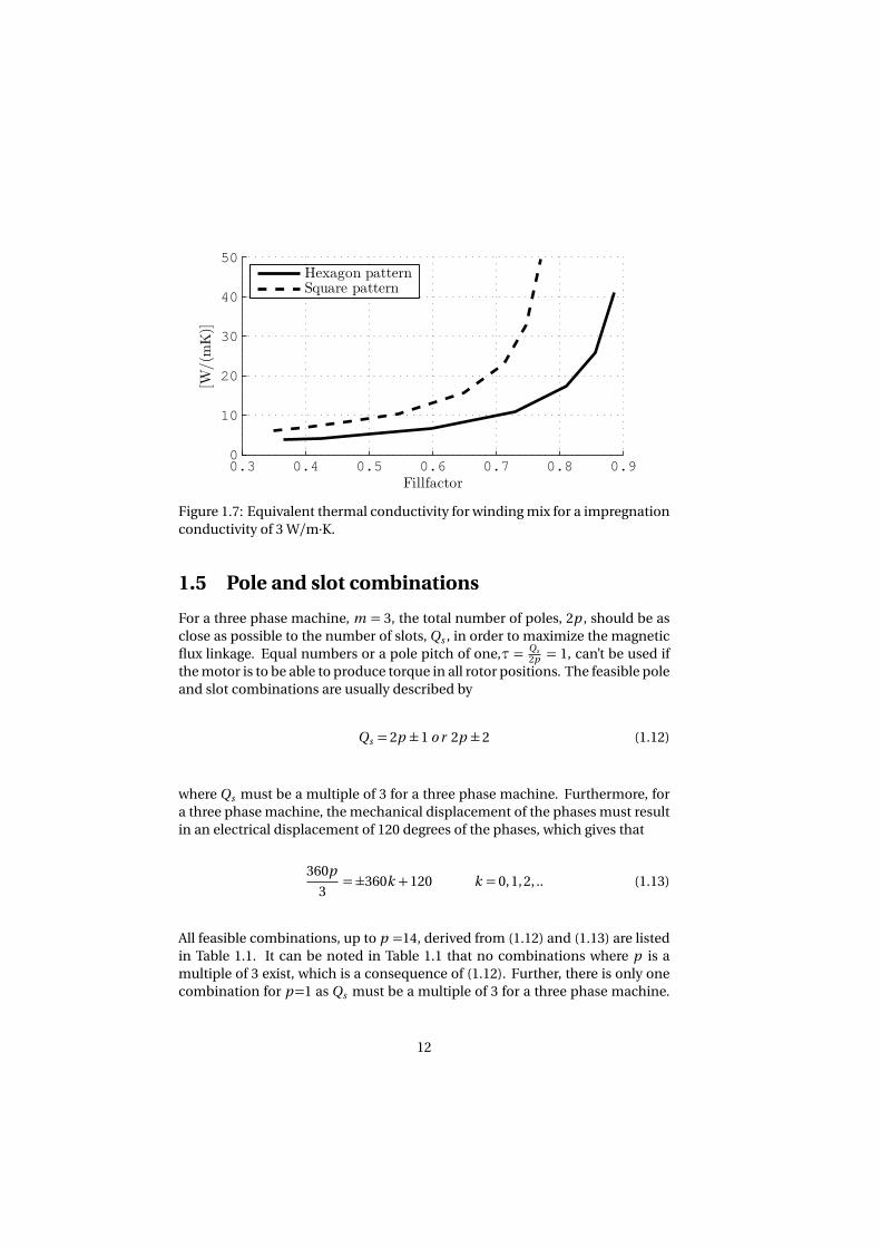
Using FEA, equivalent thermal conductivity that are calculated for hexagon and

square pattern distributions as function of the copper fill-factor are presented in

Figure 1.6 and Figure 1.7, for two different values of thermal conductivity of the

impregnation material. It can be seen that the equivalent thermal conductivi-

ties increase dramatically when the fill-factors are approaching the theoretical

maximal fill-factors, π4 ≈ 0.79 and π

2p

3≈ 0.91, for square and hexagon distribu-

tion respectively. The figures show clearly the impact of the conductor distri-

bution and the thermal conductivity of the impregnation material for all com-

binations. The impact of the fill-factor on the relative increase of the equiva-

10

lent thermal conductivity is significant at already very high fill-factors. From a

strictly thermal perspective it’s therefore beneficial to aim for even a slight in-

crease of an already very high fill-factor.

Interesting improvements of the performance at the thermal limit for two seg-

mented PMSMs using wound windings (fill-factor of 61%) and using pre-pressed

windings (fill-factor of 78%) are presented in [15]. In [16], thermal properties

for a mix of Litz wire and impregnation material, using two impregnation tech-

niques, are derived experimentally. The first sample, that was varnish dipped,

shows an equivalent thermal conductivity of 1.2-1.6 W/(m·K) while the second

sample, that was epoxi impregnated using a vacuum chamber, shows an equiv-

alent thermal conductivity of 2.9-7.4 W/(m·K).

0.3 0.4 0.5 0.6 0.7 0.8 0.90

0.5

1

1.5

2

2.5

3

Fillfactor

[W/(m

K)]

Hexagon patternSquare pattern

Figure 1.6: Equivalent thermal conductivity for winding mix for an impregna-

tion conductivity of 0.2 W/m·K.

11

0.3 0.4 0.5 0.6 0.7 0.8 0.90

10

20

30

40

50

Fillfactor

[W/(m

K)]

Hexagon patternSquare pattern

Figure 1.7: Equivalent thermal conductivity for winding mix for a impregnation

conductivity of 3 W/m·K.

1.5 Pole and slot combinations

For a three phase machine, m = 3, the total number of poles, 2p , should be as

close as possible to the number of slots, Qs , in order to maximize the magnetic

flux linkage. Equal numbers or a pole pitch of one,τ =Qs

2p = 1, can’t be used if

the motor is to be able to produce torque in all rotor positions. The feasible pole

and slot combinations are usually described by

Qs = 2p ±1 o r 2p ±2 (1.12)

where Qs must be a multiple of 3 for a three phase machine. Furthermore, for

a three phase machine, the mechanical displacement of the phases must result

in an electrical displacement of 120 degrees of the phases, which gives that

360p

3=±360k +120 k = 0, 1, 2, .. (1.13)

All feasible combinations, up to p =14, derived from (1.12) and (1.13) are listed

in Table 1.1. It can be noted in Table 1.1 that no combinations where p is a

multiple of 3 exist, which is a consequence of (1.12). Further, there is only one

combination for p=1 as Qs must be a multiple of 3 for a three phase machine.

12

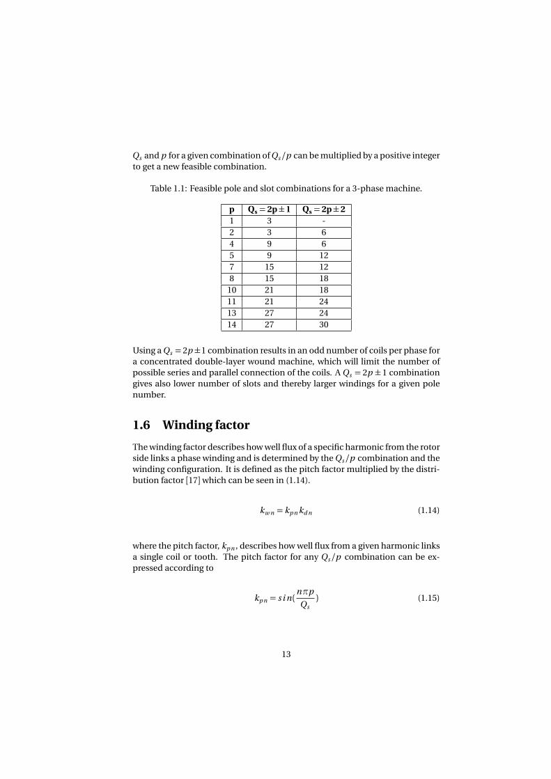
Qs and p for a given combination of Qs /p can be multiplied by a positive integer

to get a new feasible combination.

Table 1.1: Feasible pole and slot combinations for a 3-phase machine.

p Qs = 2p±1 Qs = 2p±2

1 3 -

2 3 6

4 9 6

5 9 12

7 15 12

8 15 18

10 21 18

11 21 24

13 27 24

14 27 30

Using a Qs = 2p ±1 combination results in an odd number of coils per phase for

a concentrated double-layer wound machine, which will limit the number of

possible series and parallel connection of the coils. A Qs = 2p ± 1 combination

gives also lower number of slots and thereby larger windings for a given pole

number.

1.6 Winding factor

The winding factor describes how well flux of a specific harmonic from the rotor

side links a phase winding and is determined by the Qs /p combination and the

winding configuration. It is defined as the pitch factor multiplied by the distri-

bution factor [17]which can be seen in (1.14).

kw n = kp n kd n (1.14)

where the pitch factor, kp n , describes how well flux from a given harmonic links

a single coil or tooth. The pitch factor for any Qs /p combination can be ex-

pressed according to

kp n = s i n (nπp

Qs

) (1.15)

13

where n = 1 corresponds to the fundamental of each combination [18]. The

distribution factor, kd n , is used to include the phase shift between the flux link-

age in each coil when summing up the contribution for a given harmonic in a

phase. Hence, the formulation of distribution factor is determined by both the

Qs /p combination and the winding configuration. For concentrated double-

layer windings kd n can be expressed as [18]

kd n =s i n ( nπ

2m )

z s i n ( nπ2m z )

(1.16)

where n is the harmonic number, m is the number of phases and z is the num-

ber of coils in a group. The number of coils in a group can be calculated as,

z =Qs

m F(1.17)

where F is the greatest common divisor (GCD) of the number of poles, 2p , and

the number of slots, Qs .

F =G C D (2p ,Qs ) (1.18)

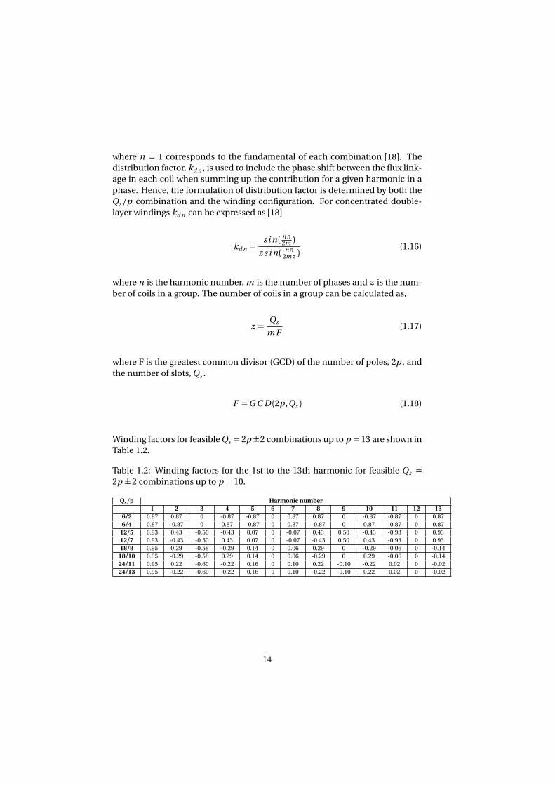
Winding factors for feasible Qs = 2p ±2 combinations up to p = 13 are shown in

Table 1.2.

Table 1.2: Winding factors for the 1st to the 13th harmonic for feasible Qs =

2p ±2 combinations up to p = 10.

Qs/p Harmonic number

1 2 3 4 5 6 7 8 9 10 11 12 13

6/2 0.87 0.87 0 -0.87 -0.87 0 0.87 0.87 0 -0.87 -0.87 0 0.87

6/4 0.87 -0.87 0 0.87 -0.87 0 0.87 -0.87 0 0.87 -0.87 0 0.87

12/5 0.93 0.43 -0.50 -0.43 0.07 0 -0.07 0.43 0.50 -0.43 -0.93 0 0.93

12/7 0.93 -0.43 -0.50 0.43 0.07 0 -0.07 -0.43 0.50 0.43 -0.93 0 0.93

18/8 0.95 0.29 -0.58 -0.29 0.14 0 0.06 0.29 0 -0.29 -0.06 0 -0.14

18/10 0.95 -0.29 -0.58 0.29 0.14 0 0.06 -0.29 0 0.29 -0.06 0 -0.14

24/11 0.95 0.22 -0.60 -0.22 0.16 0 0.10 0.22 -0.10 -0.22 0.02 0 -0.02

24/13 0.95 -0.22 -0.60 -0.22 0.16 0 0.10 -0.22 -0.10 0.22 0.02 0 -0.02

14

1.7 MMF time and space harmonics

Rotor losses caused by the induced magneto motive force (MMF) wave is men-

tioned as one of the key challenges for fractional slot machines with concen-

trated windings in [5]. As a first step the rotor losses can be lowered if the source

is minimized by a careful choice of pole slot combinations to achieve a favorable

MMF wave in the air-gap, why the calculation of time and space harmonics is of

great importance. For a given pole/slot combination, the impact of the harmon-

ics in the MMF wave can be affected by geometry and material properties. It is

possible to increase the air-gap length and introduce segmentation of the rotor

parts in order to prevent the induction of eddy currents on the rotor side. The

correlation between pole/slot combinations and rotor losses using different air-

gap lengths and rotor surface materials are investigated extensively in [6]. The

basic theory of how to analytically calculate the theoretical induced MMF har-

monics is very well described in [19] for example. In this section a conceptual

explanation follows, based on an example of the Qs = 12 machine.

The MMF wave that is induced in the air-gap when the stator is excited by cur-

rent can be described by means of MMF time and space harmonics,

F (t ,θ ) =∑

n

∑

m

Fnm s i n (mωt ±nθ +βmn ) (1.19)

where Fnm is time m:th order and space n:th order MMF magnitude. The sta-

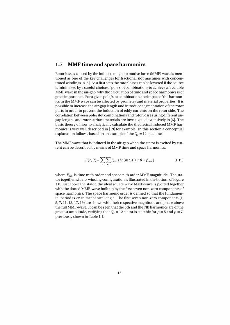
tor together with its winding configuration is illustrated in the bottom of Figure

1.8. Just above the stator, the ideal square wave MMF-wave is plotted together

with the dotted MMF-wave built up by the first seven non-zero components of

space harmonics. The space harmonic order is defined so that the fundamen-

tal period is 2π in mechanical angle. The first seven non-zero components (1,

5, 7, 11, 13, 17, 19) are shown with their respective magnitude and phase above

the full MMF-wave. It can be seen that the 5th and the 7th harmonics are of the

greatest amplitude, verifying that Qs = 12 stator is suitable for p = 5 and p = 7,

previously shown in Table 1.1.

15

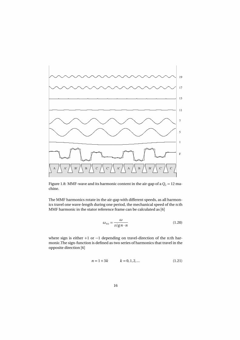
Figure 1.8: MMF-wave and its harmonic content in the air-gap of a Qs = 12 ma-

chine.

The MMF harmonics rotate in the air-gap with different speeds, as all harmon-

ics travel one wave-length during one period, the mechanical speed of the n:th

MMF harmonic in the stator reference frame can be calculated as [6]

ωn s =ω

s i g n ·n (1.20)

where sign is either +1 or −1 depending on travel-direction of the n:th har-

monic.The sign-function is defined as two series of harmonics that travel in the

opposite direction [6]

n = 1+3k k = 0, 1, 2, ... (1.21)

16

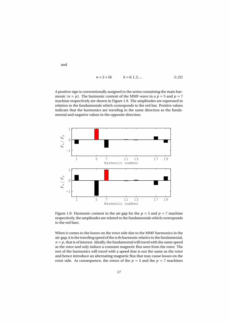
and

n = 2+3k k = 0, 1, 2, ... (1.22)

A positive sign is conventionally assigned to the series containing the main har-

monic (n = p ). The harmonic content of the MMF-wave in a p = 5 and p = 7

machine respectively are shown in Figure 1.9. The amplitudes are expressed in

relation to the fundamentals which corresponds to the red bar. Positive values

indicate that the harmonics are traveling in the same direction as the funda-

mental and negative values in the opposite direction.

1 5 7 11 13 17 19

−1

0

1

Harmonic number

Fn/F

p

1 5 7 11 13 17 19

−1

0

1

Harmonic number

Fn/F

p

Figure 1.9: Harmonic content in the air-gap for the p = 5 and p = 7 machine

respectively, the amplitudes are related to the fundamentals which corresponds

to the red bars.

When it comes to the losses on the rotor side due to the MMF harmonics in the

air-gap, it is the traveling speed of the n:th harmonic relative to the fundamental,

n = p , that is of interest. Ideally, the fundamental will travel with the same speed

as the rotor and only induce a constant magnetic flux seen from the rotor. The

rest of the harmonics will travel with a speed that is not the same as the rotor

and hence introduce an alternating magnetic flux that may cause losses on the

rotor side. As consequence, the rotors of the p = 5 and the p = 7 machines

17

will experience different harmonics when using the same stator, Qs = 12. The

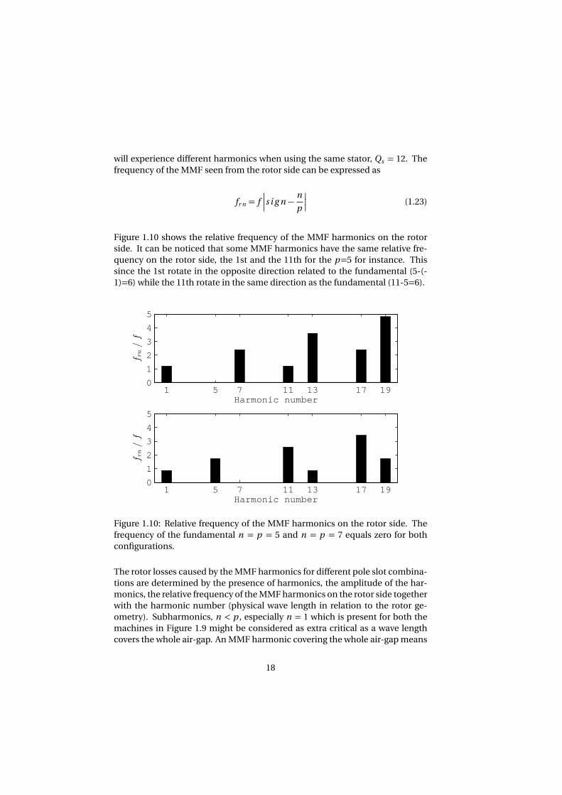
frequency of the MMF seen from the rotor side can be expressed as

fr n = f

s i g n − n

p

(1.23)

Figure 1.10 shows the relative frequency of the MMF harmonics on the rotor

side. It can be noticed that some MMF harmonics have the same relative fre-

quency on the rotor side, the 1st and the 11th for the p=5 for instance. This

since the 1st rotate in the opposite direction related to the fundamental (5-(-

1)=6) while the 11th rotate in the same direction as the fundamental (11-5=6).

1 5 7 11 13 17 190

1

2

3

4

5

Harmonic number

frn

/f

1 5 7 11 13 17 190

1

2

3

4

5

Harmonic number

frn

/f

Figure 1.10: Relative frequency of the MMF harmonics on the rotor side. The

frequency of the fundamental n = p = 5 and n = p = 7 equals zero for both

configurations.

The rotor losses caused by the MMF harmonics for different pole slot combina-

tions are determined by the presence of harmonics, the amplitude of the har-

monics, the relative frequency of the MMF harmonics on the rotor side together

with the harmonic number (physical wave length in relation to the rotor ge-

ometry). Subharmonics, n < p , especially n = 1 which is present for both the

machines in Figure 1.9 might be considered as extra critical as a wave length

covers the whole air-gap. An MMF harmonic covering the whole air-gap means

18

a flux path across the whole rotor and potentially deep flux penetration of the

rotor structure. A strategy to reduce the flux produced by an undesirable har-

monic, and thereby the losses, is to increase the reluctance of the flux path used

by that specific harmonic without affecting the flux path of the fundamental.

Introduction of different flux barriers to prevent flux caused by subharmonics

are presented in [20] and [7].

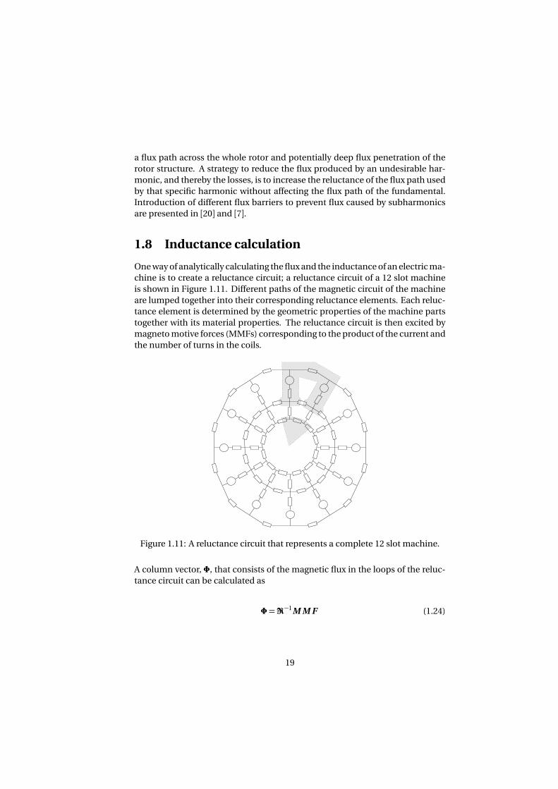
1.8 Inductance calculation

One way of analytically calculating the flux and the inductance of an electric ma-

chine is to create a reluctance circuit; a reluctance circuit of a 12 slot machine

is shown in Figure 1.11. Different paths of the magnetic circuit of the machine

are lumped together into their corresponding reluctance elements. Each reluc-

tance element is determined by the geometric properties of the machine parts

together with its material properties. The reluctance circuit is then excited by

magneto motive forces (MMFs) corresponding to the product of the current and

the number of turns in the coils.

Figure 1.11: A reluctance circuit that represents a complete 12 slot machine.

A column vector, Φ, that consists of the magnetic flux in the loops of the reluc-

tance circuit can be calculated as

Φ=ℜ−1M M F (1.24)

19

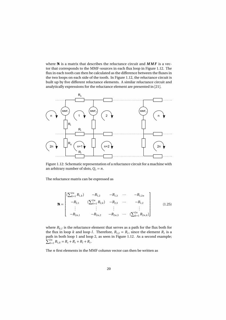
where ℜ is a matrix that describes the reluctance circuit and M M F is a vec-

tor that corresponds to the MMF-sources in each flux loop in Figure 1.12. The

flux in each tooth can then be calculated as the difference between the fluxes in

the two loops on each side of the tooth. In Figure 1.12, the reluctance circuit is

built up by five different reluctance elements. A similar reluctance circuit and

analytically expressions for the reluctance element are presented in [21].

Rt

Rs

Rl

Rg

Rr

MMF1 MMF2 MMFn

1 2 n

2nn+2n+1

n

2n

Figure 1.12: Schematic representation of a reluctance circuit for a machine with

an arbitrary number of slots, Qs = n .

The reluctance matrix can be expressed as

ℜ=

(∑2n

k=1R1,k ) −R1,2 −R1,3 · · · −R1,2n

−R2,1 (∑2n

k=1R2,k ) −R2,3 · · · −R1,2

......

......

−R2n ,1 −R2n ,2 −R2n ,3 · · · (∑2n

k=1R2n ,k )

(1.25)

where Rk ,l is the reluctance element that serves as a path for the flux both for

the flux in loop k and loop l . Therefore, R1,2 = Rt , since the element Rt is a

path in both loop 1 and loop 2, as seen in Figure 1.12. As a second example;∑2n

k=1R1,k =Rs +Rt +Rl +Rt .

The n first elements in the MMF column vector can then be written as

20

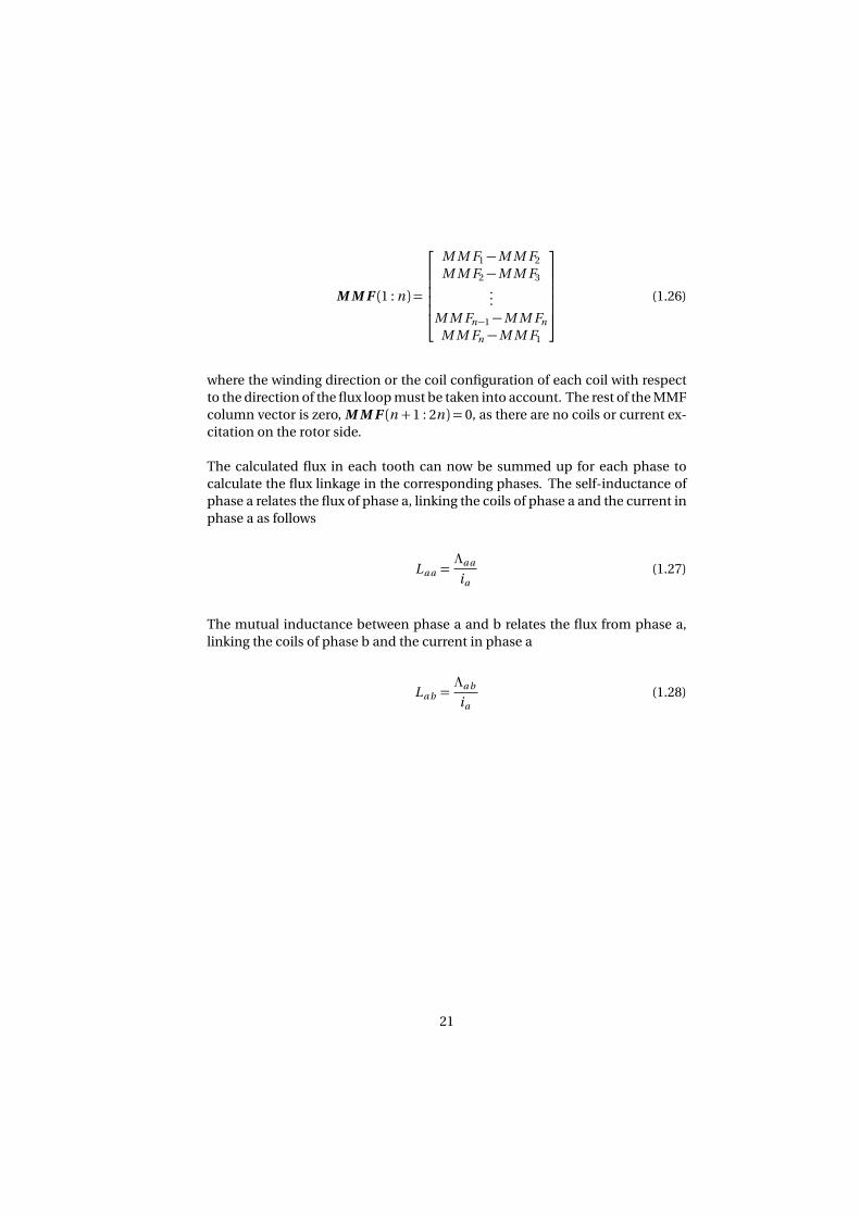
M M F (1 : n ) =

M M F1−M M F2

M M F2−M M F3

...

M M Fn−1−M M Fn

M M Fn −M M F1

(1.26)

where the winding direction or the coil configuration of each coil with respect

to the direction of the flux loop must be taken into account. The rest of the MMF

column vector is zero, M M F (n + 1 : 2n ) = 0, as there are no coils or current ex-

citation on the rotor side.

The calculated flux in each tooth can now be summed up for each phase to

calculate the flux linkage in the corresponding phases. The self-inductance of

phase a relates the flux of phase a, linking the coils of phase a and the current in

phase a as follows

La a =Λa a

ia

(1.27)

The mutual inductance between phase a and b relates the flux from phase a,

linking the coils of phase b and the current in phase a

La b =Λa b

ia

(1.28)

21

22

Chapter 2

Dynamic Modeling of PMSMs

This chapter deals with the the dynamic modeling of PMSMs under balanced

and unbalanced or faulty conditions. Although this licentiate thesis focuses on

the design of a fault-tolerant PMSM, the unbalanced conditions impose addi-

tional requirements of the controller and the converter. Both a controller and

some converter topologies that can handle the unbalanced operation are there-

fore presented. The reader is expected to be familiar with general machine mod-

eling and the transformations between the different reference frames that are

associated with both machine modeling and control, which are well described

in [22] for example.

2.1 Basic 3ph-model

The electrical equations, expressing the phase voltages of a three phase PMSM

can be written on matrix form as

va

vb

vc

=

L s a L s a b L s a c

L s a b L s b L s b c

L s a c L s b c L s c

d

d t

ia

ib

ic

+

Rs 0 0

0 Rs 0

0 0 Rs

ia

ib

ic

+

ea

eb

ec

(2.1)

where ea , eb and ec are the back EMF terms of each phase. If the flux from the

permanent magnets are considered to be sinusoidal and symmetrically placed

towards each other, the back EMF terms can be formulated as

23

ea

eb

ec

=ωΨm

c o s (θ )

c o s (θ − 2π3 )

c o s (θ − 4π3 )

(2.2)

where ω is the electric angular frequency and Ψm is the magnitude of the flux

linkage in a phase. Further, the self inductance of the phases are equal and they

can be denoted

L s a = L s b = L s c = L (2.3)

Also the mutual coupling between all phases are the same and it can be denoted

L s a b = L s a c = L s b c =M (2.4)

For a balanced three phase system where ia+ib +ic = 0 and utilizing L s = L−M ,

(2.1) can be rewritten as

va

vb

vc

=

L s 0 0

0 L s 0

0 0 L s

d

d t

ia

ib

ic

+

Rs 0 0

0 Rs 0

0 0 Rs

ia

ib

ic

+

ea

eb

ec

(2.5)

For a machine without rotor saliency, the inductance is not dependent on the

rotor position and no reluctance torque can be created. Hence, the electrody-

namic torque can be expressed as

Te =ia ea

Ω+

ib eb

Ω+

ic ec

Ω(2.6)

where Ω represents the mechanical angular frequency.

24

2.2 Flux model in the rotating dq-reference frame

In the rotating dq reference frame, the stator voltage of a PMSM can be ex-

pressed as

ud =Rs id + Ld

d id

d t−ωLq iq (2.7)

uq =Rs iq + Ld iq

d t+ωLd id +ωΨm (2.8)

where only the fundamental frequency component is considered and the per-

manent magnet flux is oriented in the direct axis. The electrodynamic torque

can be written as

Te =ψd iq −ψq id (2.9)

If the flux components are expressed as ψd = Ψm + Ld id and ψq = Lq iq , the

torque equation (2.9) can be rewritten as

Te =Ψm iq + (Ld − Lq )id iq (2.10)

which is a widely used expression. Using this model for a non-linear machine,

it is problematic to divide the direct axis flux, ψd , into its PM flux component,

Ψm and its induced flux component, Ld id . Both Ψm and Ld id share the same

non-linear flux paths, as previously shown in Figure 1.2 in Section 1.1. Conse-

quently, both Ψm and L are functions of the currents, id and iq , and it is thereby

possible to divideψd in an infinite number of combinations of Ψm and Ld id if

no further assumptions are introduced.

Another possibility is to model the PMSM based on the flux including all har-

monics without dividing the direct axis flux into PM and induced flux. The flux

in the direct and quadrature axis is a function of the currents and the rotor po-

sition respectively

ψd =ψd (id , iq ,θ ) (2.11)

ψq =ψq (id , iq ,θ ) (2.12)

25

where the rotor angle, θ , must be varied within an interval determined by the

pole/slot combination and winding configuration. Equation (2.11) and (2.12)

are rather impractical since the fluxes vary in three dimensions. If only consid-

ering the fundamental frequency and a steady-state operating point, (2.7) and

(2.14) can be rewritten as

ud =Rs id −ωΨq (2.13)

uq =Rs iq +ωΨd (2.14)

where bothΨd andΨq represent the amplitudes of the fundamental component

of the flux linkage in the direct and quadrature axis respectively. A set of Ψd and

Ψq as function of id and iq can be calculated by means of FEA, using (2.13) and

(2.14). Thus, the fundamental phase voltage at a steady-state operating point

can be found accurately.

2.3 Basic modeling of chosen faults

The three phase model presented in (2.1) can be written on the general state

space form

x = Ax +B u (2.15)

y =C x +D u (2.16)

In the state space model of the machine, the currents represent the states, the

current derivatives the state derivatives, while the input voltage is used as input

and it becomes

d i

d t=−i n v (L )R i + i n v (L )v − i n v (L )e (2.17)

The corresponding A and B can then be expressed as

A =−i n v (L )R (2.18)

B = i n v (L ) (2.19)

26

The three phase model can then be implemented as follows

d

d t

ia

ib

ic

= A

ia

ib

ic

+B

va

vb

vc

−B

ea

eb

ec

(2.20)

where

A =

A11 A12 A13

A21 A22 A23

A31 A32 A33

(2.21)

and

B =

B11 B12 B13

B21 B22 B23

B31 B32 B33

(2.22)

which is referred to in the following sections, where it has been manipulated to

include phase open and phase short circuit faults.

2.3.1 Phase short circuit

The suggested phase short circuit fault manipulation of (2.20) is probably the

most straightforward. The terminal phase voltage of the faulty phase, vi , is sim-

ply put to zero. Characteristics of the short circuit connection might be added

by manipulation of the R and L matrices if desired.

2.3.2 Phase open circuit

Two different ways of phase open circuit manipulation are presented. The first

changes instantaneously from normal operation to phase open circuit opera-

tion while the second takes the transition into account.

State and energy removed

In the most simple approach, the simulation stops when a fault occurs. The

states in the machine model (and possible other states such as values in the

integrator parts of controllers) are saved. The model is then changed, the state

that represents the faulty phase is removed. The saved states are then used as

27

initial conditions when starting the simulation of the new model that represents

the characteristics after the fault occurred. As a consequence, energy is removed

when the state corresponding to current in the faulty phase is removed.

State and energy conserved

As a second approach , the state corresponding to the current in the faulty phase

is controlled to zero; instead of just put the current in the faulty phase to zero

and thereby removing the energy instantaneously. From a simulation perspec-

tive it is beneficial to control the current to interrupt like a first order system,

see Figure 2.1. The voltage that has to build up over the phase winding is calcu-

lated and used as input signal to the state space model, where all states still are

remaining.

xr e f xF (s )

ǫ 1

s

x

Figure 2.1: Illustration of how the derivative of the state can be controlled.

To get the behavior of a first order system, from the state reference, xr e f , to the

state value, x , it can be shown that F (s ) = α, where α is the bandwidth of the

first order system. The state derivative, representing the faulty phase, in the

state space model can then be expressed as

x =α(xr e f − x ) (2.23)

when a fault occurs. The voltage that must build up over the phase winding

(phase c is used in this case) is calculated as

vc =α(0− ic )−A(3, 1 : 3)i (1 : 3)−B (3, 1 : 2)u (1 : 2) +B (3, 1 : 3)e (1 : 3)

b (3, 3)(2.24)

28

2.4 Control

This section presents the two controllers, in the rotating dq0 reference frame,

that are used in this thesis. The ordinary PI controller, that are suitable for bal-

anced three phase control are not explained in detail as it is very well established

within electric machine control. Adding a resonant controller in parallel with an

existing PI controller is proposed when operating the machine under faulty and

unsymmetrical conditions.

2.4.1 Ordinary PI controller

When the ordinary PI controller is used in the dq0 reference frame, the rotating

three phase quantities are transformed to stationary quantities in the rotating

dq0 reference frame via the stationary αβ0 reference frame. In case of a bal-

anced three phase system in steady-state, all the dq0-components will appear

as DC-values which the PI controller is well adapted for. The PI controller is rep-

resented as the lower part in the combined resonant and PI controller in Figure

2.2 in section 2.4.2.

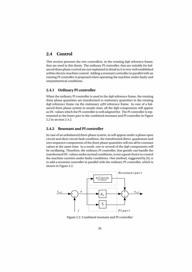
2.4.2 Resonant and PI controller

In case of an unbalanced three phase system, as will appear under a phase open

circuit and short circuit fault condition, the transformed direct, quadrature and

zero sequence components of the three phase quantities will not all be constant

values at the same time. As a result, one or several of the dq0-components will

be oscillating. Therefore, the ordinary PI controller, that greatly can handle the

transformed DC-values under normal conditions, is not a good choice to control

the machine currents under faulty conditions. One method, suggested by [9], is

to add a resonant controller in parallel with the ordinary PI-controller, which is

shown in Figure 2.2.

a2 s 2+a1 s+a0

s 2+(hω)2

ir e f vr e f

i

Kp

Ki

s

ǫ

R e s o na n t p a r t

P I p a r t

Figure 2.2: Combined resonant and PI controller

29

In case of a machine with surface mounted permanent magnets and no rotor

saliency, no reluctance torque is expected as Ld = Lq , and it is only necessary to

keep the torque producing q-component of the current constant. On the other

hand, for a machine with a difference between the direct and quadrature axis

inductance it is also necessary to hold the d-component of the current constant.

The proposed current controller will force both the q and the d components of

the current to constant values, while the zero sequence component that does

not produce torque is left oscillating.

2.5 Converter limitations

Using the ordinary three leg converter that is shown in Figure 2.3a, it is not pos-

sible to control the phase currents individually in case of a phase open circuit or

a phase short circuit. The current into one of the remaining phases must equal

the current that goes out from the second healthy phase. Three alternative con-

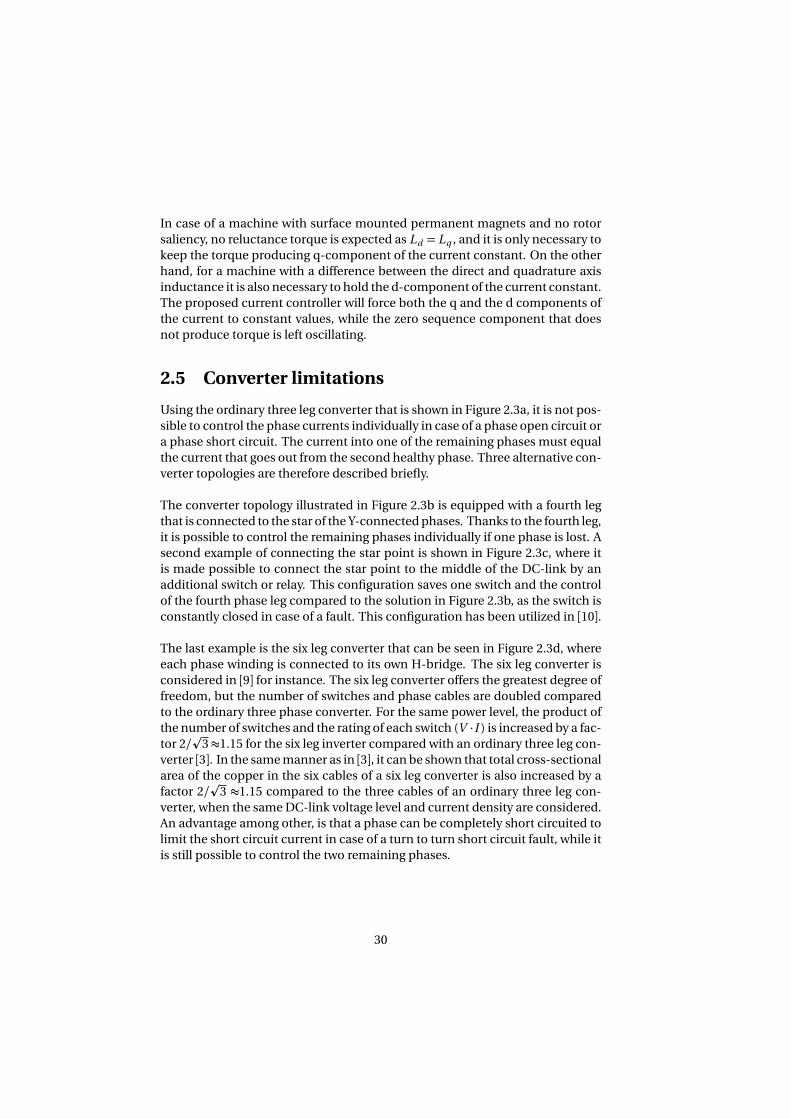
verter topologies are therefore described briefly.

The converter topology illustrated in Figure 2.3b is equipped with a fourth leg

that is connected to the star of the Y-connected phases. Thanks to the fourth leg,

it is possible to control the remaining phases individually if one phase is lost. A

second example of connecting the star point is shown in Figure 2.3c, where it

is made possible to connect the star point to the middle of the DC-link by an

additional switch or relay. This configuration saves one switch and the control

of the fourth phase leg compared to the solution in Figure 2.3b, as the switch is

constantly closed in case of a fault. This configuration has been utilized in [10].

The last example is the six leg converter that can be seen in Figure 2.3d, where

each phase winding is connected to its own H-bridge. The six leg converter is

considered in [9] for instance. The six leg converter offers the greatest degree of

freedom, but the number of switches and phase cables are doubled compared

to the ordinary three phase converter. For the same power level, the product of

the number of switches and the rating of each switch (V ·I ) is increased by a fac-

tor 2/p

3≈1.15 for the six leg inverter compared with an ordinary three leg con-

verter [3]. In the same manner as in [3], it can be shown that total cross-sectional

area of the copper in the six cables of a six leg converter is also increased by a

factor 2/p

3 ≈1.15 compared to the three cables of an ordinary three leg con-

verter, when the same DC-link voltage level and current density are considered.

An advantage among other, is that a phase can be completely short circuited to

limit the short circuit current in case of a turn to turn short circuit fault, while it

is still possible to control the two remaining phases.

30

a) b)

c) d)

Figure 2.3: Four different converter topologies.

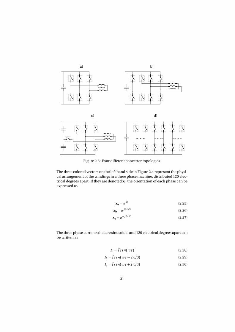
The three colored vectors on the left hand side in Figure 2.4 represent the physi-

cal arrangement of the windings in a three phase machine, distributed 120 elec-

trical degrees apart. If they are denoted xi, the orientation of each phase can be

expressed as

xa = e j 0 (2.25)

xb = e j 2π/3 (2.26)

xc = e − j 2π/3 (2.27)

The three phase currents that are sinusoidal and 120 electrical degrees apart can

be written as

Ia = I s i n (w t ) (2.28)

Ib = I s i n (w t −2π/3) (2.29)

Ic = I s i n (w t +2π/3) (2.30)

31

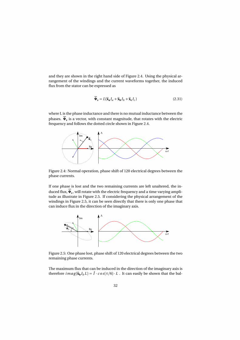
and they are shown in the right hand side of Figure 2.4. Using the physical ar-

rangement of the windings and the current waveforms together, the induced

flux from the stator can be expressed as

Ψs = L (xaIa +xbIb +xcIc ) (2.31)

where L is the phase inductance and there is no mutual inductance between the

phases. Ψs is a vector, with constant magnitude, that rotates with the electric

frequency and follows the dotted circle shown in Figure 2.4.

Im

Re

A

ωt

Ψs

Figure 2.4: Normal operation, phase shift of 120 electrical degrees between the

phase currents.

If one phase is lost and the two remaining currents are left unaltered, the in-

duced flux, Ψs , will rotate with the electric frequency and a time varying ampli-

tude as illustrate in Figure 2.5. If considering the physical arrangement of the

windings in Figure 2.5, it can be seen directly that there is only one phase that

can induce flux in the direction of the imaginary axis.

Im

Re

A

ωt

Ψs

Figure 2.5: One phase lost, phase shift of 120 electrical degrees between the two

remaining phase currents.

The maximum flux that can be induced in the direction of the imaginary axis is

therefore i ma g (xbIb L ) = I · c o s (π/6) · L . It can easily be shown that the bal-

32

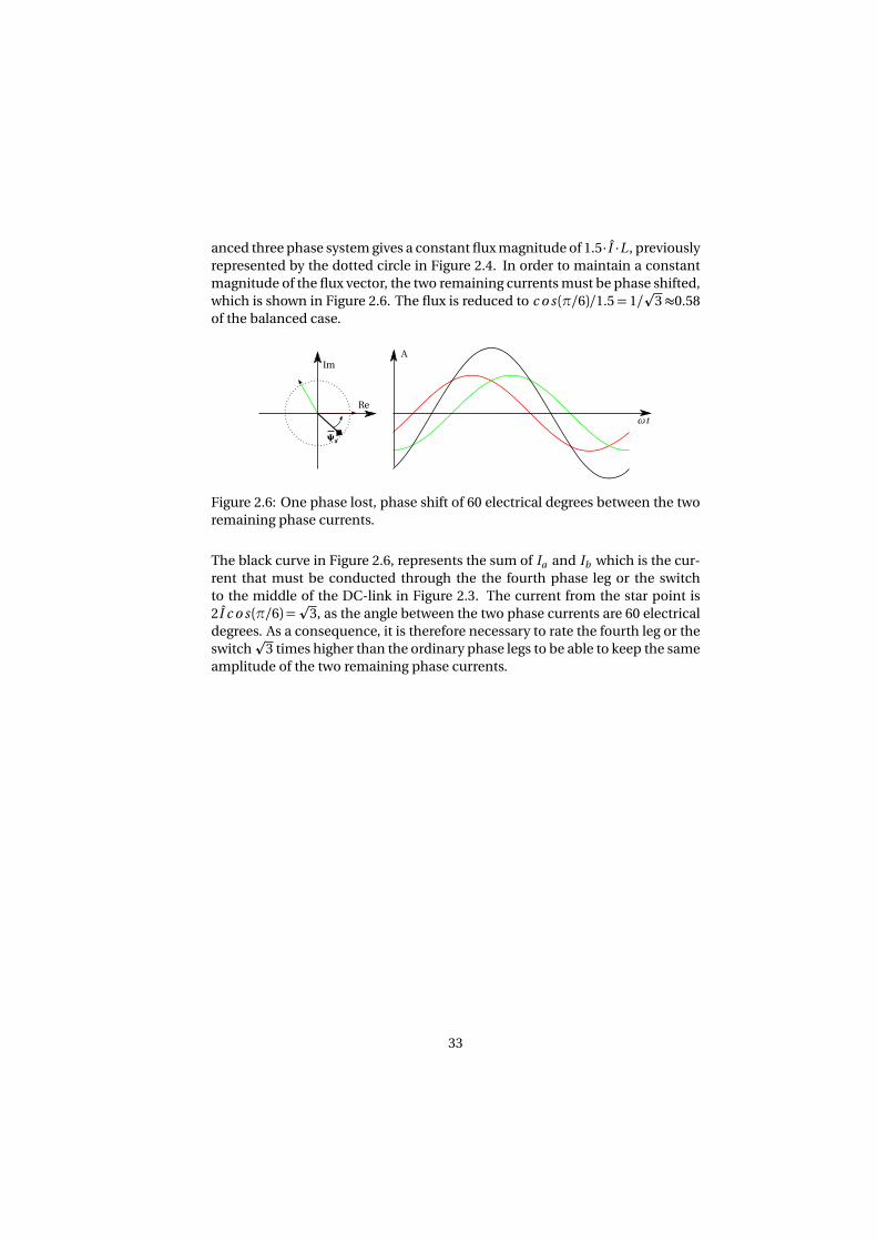
anced three phase system gives a constant flux magnitude of 1.5· I ·L , previously

represented by the dotted circle in Figure 2.4. In order to maintain a constant

magnitude of the flux vector, the two remaining currents must be phase shifted,

which is shown in Figure 2.6. The flux is reduced to c o s (π/6)/1.5= 1/p

3≈0.58

of the balanced case.

Im

Re

A

ωt

Ψs

Figure 2.6: One phase lost, phase shift of 60 electrical degrees between the two

remaining phase currents.

The black curve in Figure 2.6, represents the sum of Ia and Ib which is the cur-

rent that must be conducted through the the fourth phase leg or the switch

to the middle of the DC-link in Figure 2.3. The current from the star point is

2I c o s (π/6) =p

3, as the angle between the two phase currents are 60 electrical

degrees. As a consequence, it is therefore necessary to rate the fourth leg or the

switchp

3 times higher than the ordinary phase legs to be able to keep the same

amplitude of the two remaining phase currents.

33

34

Chapter 3

Design of fault-tolerant

fractional slot machines

Chapter 3 describes how the theory in Chapter 1 has been implemented when

the factional slot machines are designed. The chapter starts with an introduc-

tion of the design specification, that is based on the Toyota Prius Machine from

2004. A choice of pole/slot configurations is presented, while the final analysis

of the designs are left to Chapter 4.

3.1 Design specification

The design specification has been chosen based on the physical dimensions of

the Toyota Prius Machine from 2004, in order to design a fractional slot ma-

chine of similar physical size including the active parts. The Prius 2004 machine

has been used as a reference as it has been investigated intensively and a lot of

reference material is currently available. The end-windings are expected to be

shorter for a fractional slot machine with concentrated windings compared to

a machine with distributed windings. It has been assumed that the stator stack

length can be extended by approximately 30%. In fact, the protrusion of the end-

windings varies depending on many things; slot geometry, copper wires, man-

ufacturing process etc. An interesting study, where the size of the end-windings

are compared when the same stator is wound with; distributed windings, one-

layer concentrated winding and two-layer concentrated winding is presented

by [23]. More about estimation of the end-windings of the final designs can be

found in Section 4.2.1. Some key parameters of the 2004 Prius are presented

together with the design specification of the thesis design in Table 3.1.

35

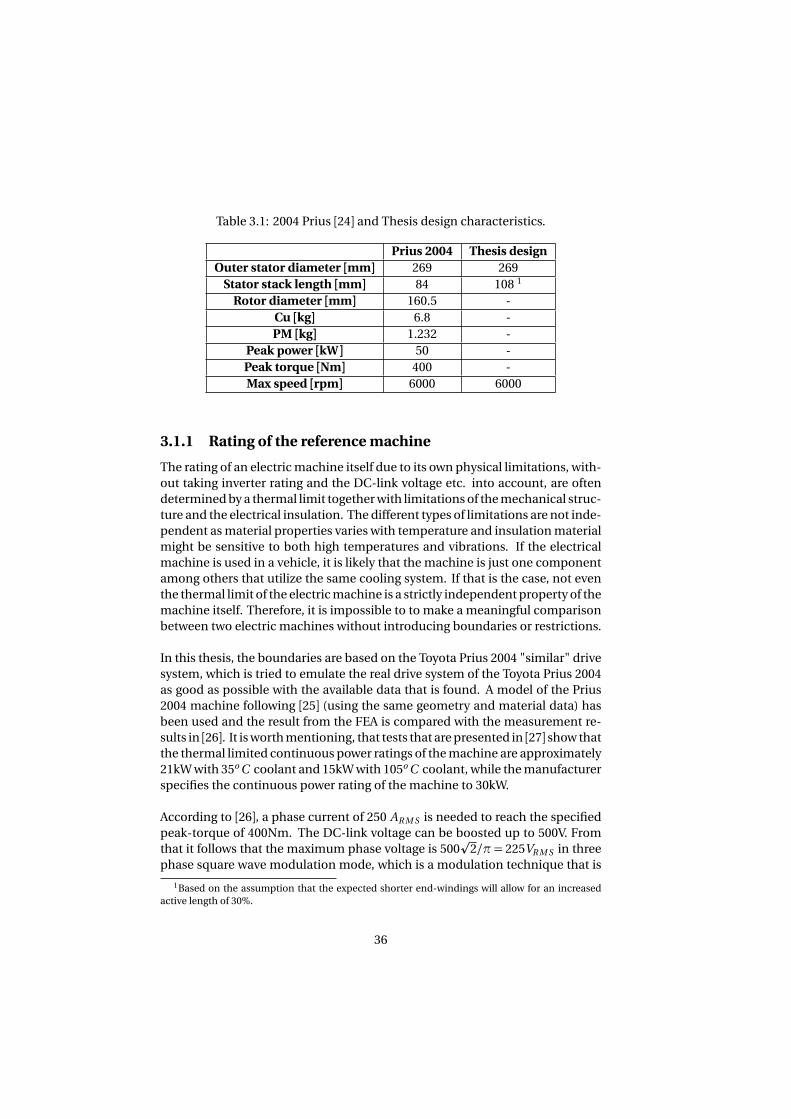
Table 3.1: 2004 Prius [24] and Thesis design characteristics.

Prius 2004 Thesis design

Outer stator diameter [mm] 269 269

Stator stack length [mm] 84 108 1

Rotor diameter [mm] 160.5 -

Cu [kg] 6.8 -

PM [kg] 1.232 -

Peak power [kW] 50 -

Peak torque [Nm] 400 -

Max speed [rpm] 6000 6000

3.1.1 Rating of the reference machine

The rating of an electric machine itself due to its own physical limitations, with-

out taking inverter rating and the DC-link voltage etc. into account, are often

determined by a thermal limit together with limitations of the mechanical struc-

ture and the electrical insulation. The different types of limitations are not inde-

pendent as material properties varies with temperature and insulation material

might be sensitive to both high temperatures and vibrations. If the electrical

machine is used in a vehicle, it is likely that the machine is just one component

among others that utilize the same cooling system. If that is the case, not even

the thermal limit of the electric machine is a strictly independent property of the

machine itself. Therefore, it is impossible to to make a meaningful comparison

between two electric machines without introducing boundaries or restrictions.

In this thesis, the boundaries are based on the Toyota Prius 2004 "similar" drive

system, which is tried to emulate the real drive system of the Toyota Prius 2004

as good as possible with the available data that is found. A model of the Prius

2004 machine following [25] (using the same geometry and material data) has

been used and the result from the FEA is compared with the measurement re-

sults in [26]. It is worth mentioning, that tests that are presented in [27] show that

the thermal limited continuous power ratings of the machine are approximately

21kW with 35o C coolant and 15kW with 105o C coolant, while the manufacturer

specifies the continuous power rating of the machine to 30kW.

According to [26], a phase current of 250 AR M S is needed to reach the specified

peak-torque of 400Nm. The DC-link voltage can be boosted up to 500V. From

that it follows that the maximum phase voltage is 500p

2/π = 225VR M S in three

phase square wave modulation mode, which is a modulation technique that is

1Based on the assumption that the expected shorter end-windings will allow for an increased

active length of 30%.

36

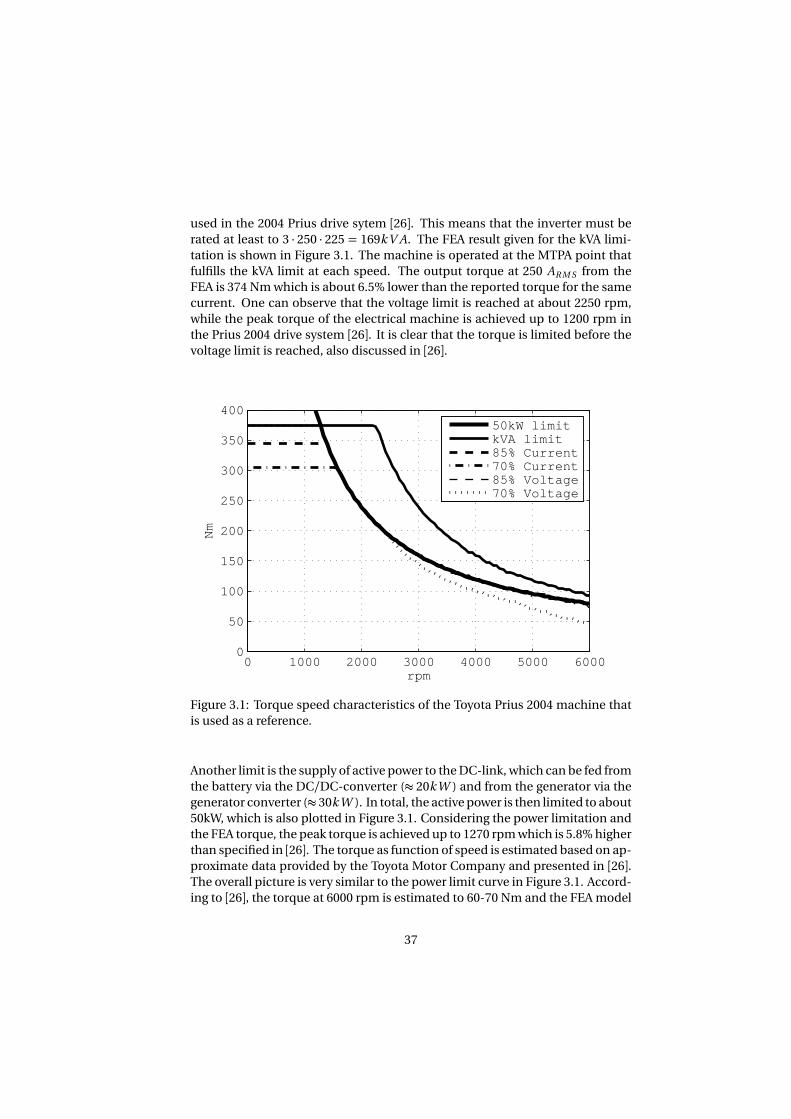
used in the 2004 Prius drive sytem [26]. This means that the inverter must be

rated at least to 3 · 250 · 225 = 169k V A. The FEA result given for the kVA limi-

tation is shown in Figure 3.1. The machine is operated at the MTPA point that

fulfills the kVA limit at each speed. The output torque at 250 AR M S from the

FEA is 374 Nm which is about 6.5% lower than the reported torque for the same

current. One can observe that the voltage limit is reached at about 2250 rpm,

while the peak torque of the electrical machine is achieved up to 1200 rpm in

the Prius 2004 drive system [26]. It is clear that the torque is limited before the

voltage limit is reached, also discussed in [26].

0 1000 2000 3000 4000 5000 60000

50

100

150

200

250

300

350

400

Nm

rpm

50kW limitkVA limit85% Current70% Current85% Voltage70% Voltage

Figure 3.1: Torque speed characteristics of the Toyota Prius 2004 machine that

is used as a reference.

Another limit is the supply of active power to the DC-link, which can be fed from

the battery via the DC/DC-converter (≈ 20k W ) and from the generator via the

generator converter (≈ 30k W ). In total, the active power is then limited to about

50kW, which is also plotted in Figure 3.1. Considering the power limitation and

the FEA torque, the peak torque is achieved up to 1270 rpm which is 5.8% higher

than specified in [26]. The torque as function of speed is estimated based on ap-

proximate data provided by the Toyota Motor Company and presented in [26].

The overall picture is very similar to the power limit curve in Figure 3.1. Accord-

ing to [26], the torque at 6000 rpm is estimated to 60-70 Nm and the FEA model

37

shows about 75 Nm at the same speed.

In addition to the active power and kVA limit of the converter found, the sen-

sitivity of the relatively high kVA limit was studied and presented in Figure 3.1.

The voltage and current limits of the converter were reduced in two steps re-

spectively (to 85% and to 70%). The effect of the current reduction (voltage at

100%) can be seen in the low speed region only, the torque is reduced and the

speed limit of the peak torque is increased as a direct consequence of the power

limit. The torque output is not affected when the current is put back to 100%

and the voltage reduced to 85%, as the torque is still limited by the active power

and not the voltage. If the voltage is reduced to 70%, the torque is voltage limited

from approximately 2500 rpm, while it is power limited in the range 1270-2500

rpm and current limited in the range 0-1270 rpm.

It should be noted that a set of id and iq combinations exists for each speed and

torque level, where the shortest current vector corresponds to the MTPA operat-

ing point. When the voltage was reduced to 85%, it is still possible that a subset

of id and iq combinations including the original MTPA operating point is dis-

qualified due to voltage limitation and a new MTPA operating point that fulfills

the voltage limitation is found. This can not be seen in the torque speed dia-

gram in Figure 3.1, as the same torque level is maintained. This is an interesting

aspect when it comes to turn selections of the machines. It might be possible to

choose a high number of turns without limitation of the torque at higher speeds

as it is limited by active power rather than voltage. On the other hand, it is possi-

ble that a higher number of turns will results in an increased transfer of reactive

power between the converter and the machine as the power factor is affected.

3.2 Selection of pole and slot combination

Some feasible pole and slot combinations were previously shown in Table 1.1,

where both Qs = 2p ± 1 and Qs = 2p ± 2 combinations were presented. The

Qs = 2p ±1 combinations results in an odd number of slots and teeth per phase

which is not regarded as a suitable choice for a fault tolerant machine, as the

sum of the induced flux per phase cannot be zero. For all the Qs = 2p ± 1 com-

binations, the flux from one phase must link to another phase and it will result

in a considerable mutual inductance between the phases.

Remaining are the Qs = 2p ± 2 combinations, which result in an even number

of teeth per phase and possibly a very low mutual coupling between phases de-

pending on the winding configuration. Back-EMF phasor diagrams for Qs =

2p ±2 combinations from p = 5 to p = 13 are shown in Table 3.2. It can be seen

that machines with the same number of slots, Qs , will result in the same winding

38

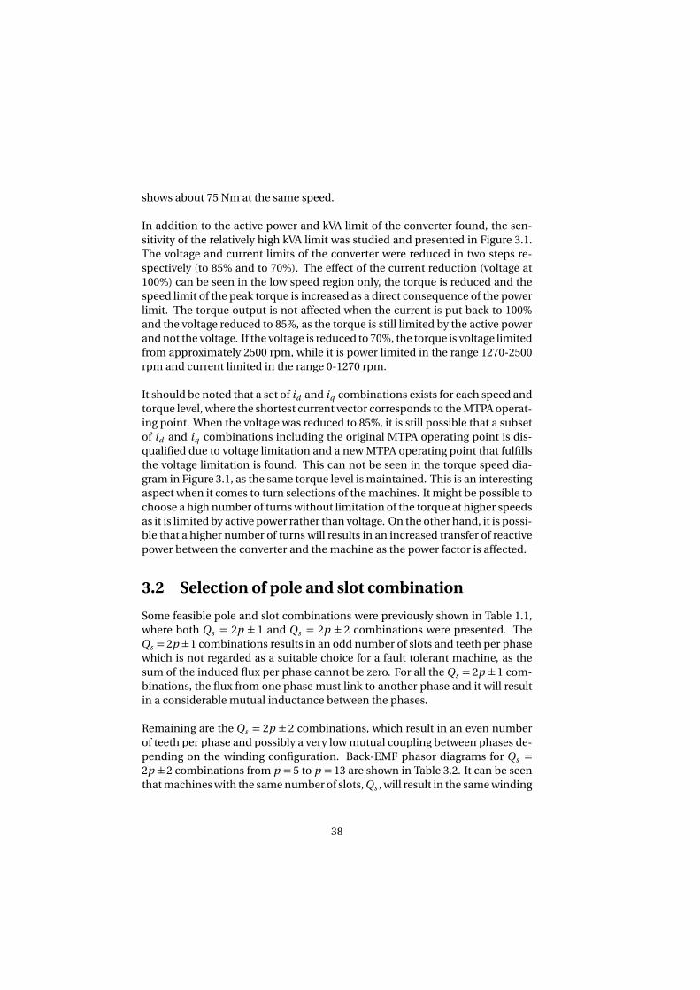
configuration as the phasor diagrams are just mirrored.

Table 3.2: Back-EMF phasor diagrams.

12/5 12/7

18/8 18/10

24/11 24/13

Models of the resulting three stator configurations that might be of interest are

39

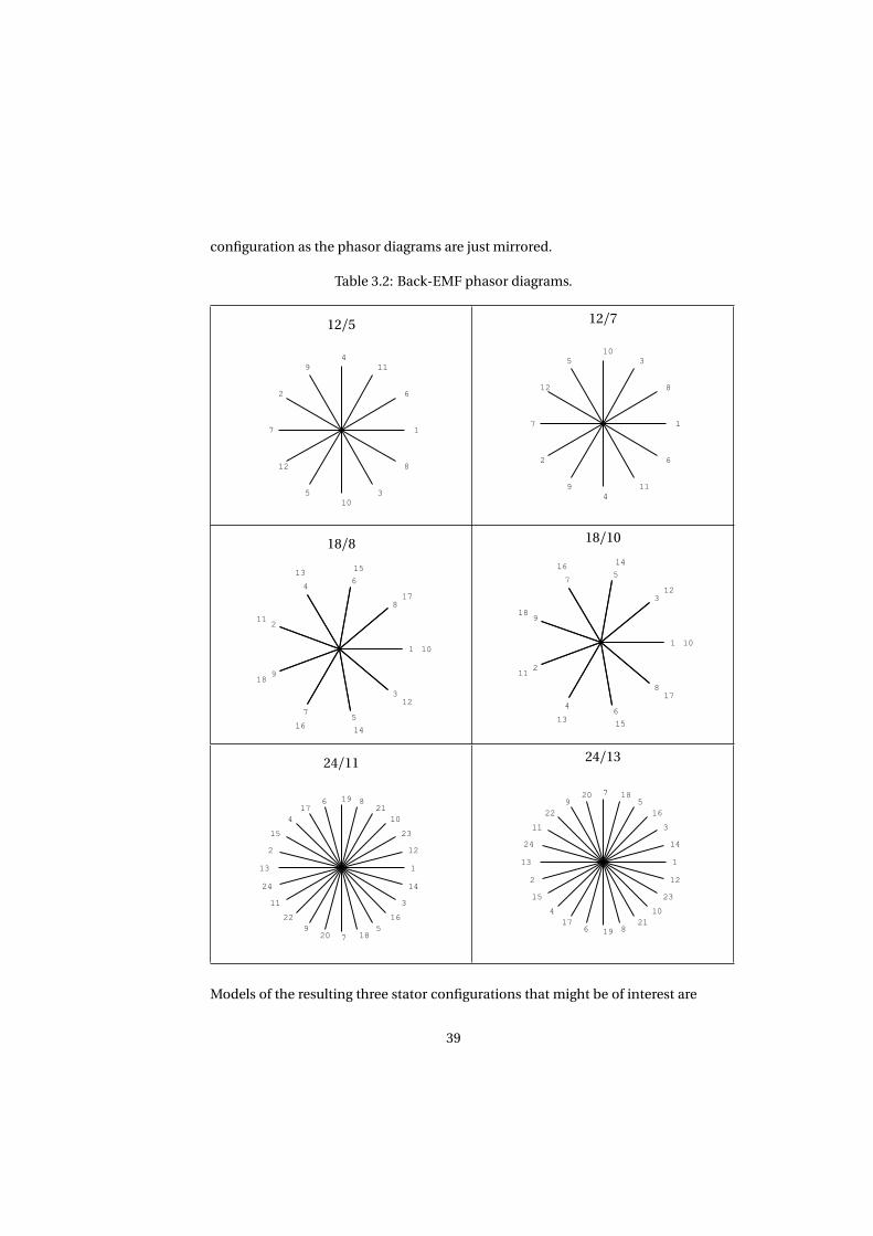
created in FEA models and are shown in Figure 3.2. No permanent magnets are

introduced, the rotors are just solid iron cores, and the stators are excited ac-

cording to their respective winding configuration. The grey or shadowed areas

represents the teeth of one phase in each stator configuration. It can be seen

that groups of an even number of teeth, 2 and 4, appear for the 12/5 and 24/11

configurations while the 18/8 configuration shows groups of an odd number, 3.

One can conclude that the phases of the 18/8 configuration are harder magnet-

ically coupled than for the other two configurations. The local sum of the flux

from an odd group of teeth cannot be zero, thus more flux lines from the grey

teeth link the neighboring teeth, see Figure 3.2. Therefore, only the Qs = 12 and

Qs = 24 are finally regarded as interesting choices.

12/5 18/8 24/11

Figure 3.2: Flux lines representing induced flux for three different pole slot com-

binations.

Another interesting aspect when studying Figure 3.2, is that the lowest possi-

ble MMF subharmonic with a wave length that equals 2π mechanical rad can

be seen. It causes the flux lines that crosses straight through the rotor and is

present in the Qs = 12 and Qs = 24 but not in the Qs = 18 stator configuration.

The MMF harmonics of the 12/5 and 12/7 configurations have already been

used as an example in section 1.7 and are presented in Figure 1.9. It is clear

that the 12/5 arrangement provides a more advantageous MMF harmonics pat-

tern in relation to the fundamental. The two pole configurations are compared

when used in an axial flux machine configuration in [28]. In that case the rotor

losses for the p = 7 is about twice compared to the p = 5. Their winding factors

are the same and p = 5 is therefore considered for the Qs = 12 configuration.

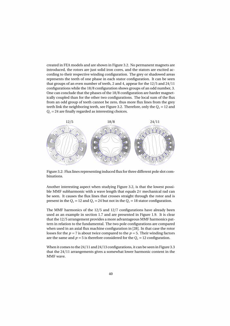
When it comes to the 24/11 and 24/13 configurations, it can be seen in Figure 3.3

that the 24/11 arrangements gives a somewhat lower harmonic content in the

MMF wave.

40

1 5 7 11 13 17 19

−1

0

1

Harmonic number

Fn/F

p

1 5 7 11 13 17 19

−1

0

1

Harmonic number

Fn/F

p

Figure 3.3: Harmonic content in the air-gap for the p = 11 and p = 13 ma-

chine respectively. The amplitudes are related to the fundamentals which cor-

responds to the red bars.

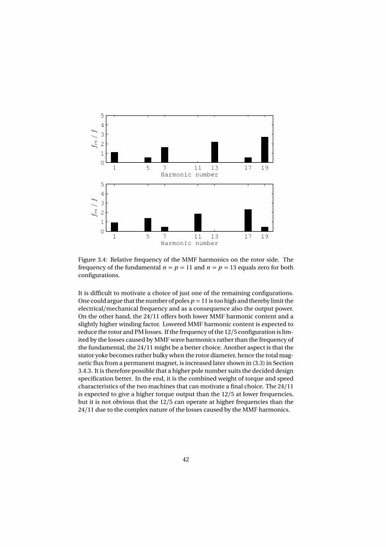
The relative frequency of the MMF harmonics on the rotor side are shown in

Figure 3.4. It can be seen that the relative frequency of the fundamental com-

ponent is zero in both configurations and that the relative frequency of the 5th

and 7th harmonics is shifted somehow, in a similar way as the 17th and 19th. As

the winding factors are the same for both pole numbers but the pole numbers

are relatively high, the p = 11 is considered for the Qs = 24 configuration.

41

1 5 7 11 13 17 190

1

2

3

4

5

Harmonic number

frn

/f

1 5 7 11 13 17 190

1

2

3

4

5

Harmonic number

frn

/f

Figure 3.4: Relative frequency of the MMF harmonics on the rotor side. The

frequency of the fundamental n = p = 11 and n = p = 13 equals zero for both

configurations.

It is difficult to motivate a choice of just one of the remaining configurations.

One could argue that the number of poles p = 11 is too high and thereby limit the

electrical/mechanical frequency and as a consequence also the output power.

On the other hand, the 24/11 offers both lower MMF harmonic content and a

slightly higher winding factor. Lowered MMF harmonic content is expected to

reduce the rotor and PM losses. If the frequency of the 12/5 configuration is lim-

ited by the losses caused by MMF wave harmonics rather than the frequency of

the fundamental, the 24/11 might be a better choice. Another aspect is that the

stator yoke becomes rather bulky when the rotor diameter, hence the total mag-

netic flux from a permanent magnet, is increased later shown in (3.3) in Section

3.4.3. It is therefore possible that a higher pole number suits the decided design

specification better. In the end, it is the combined weight of torque and speed

characteristics of the two machines that can motivate a final choice. The 24/11

is expected to give a higher torque output than the 12/5 at lower frequencies,

but it is not obvious that the 12/5 can operate at higher frequencies than the

24/11 due to the complex nature of the losses caused by the MMF harmonics.

42

3.3 FEA and material data

This section presents how the FEA has been carried out through the thesis work

and also the data that have been used.

3.3.1 Finite Element Analysis

The electromagnetic part of the finite element analysis has been carried out in

ANSYS Maxwell v.15, while the thermal part of the finite element analysis has

been carried out in femm 4.2. Except for Figure 3.2 that is produced for illus-

trative purpose only, in femm 4.2. All models are created based on 2D geome-

tries, where the electromagnetic part is carried out in static as well as in transient

modeling mode. The thermal modeling is made only in static mode and rather

simplified models has been used.

3.3.2 Material data

Copper

In the FEA, the current is modeled to be uniform through the 2D winding ob-

ject. The current density in the winding object has been scaled according to the

fill-factor and the slot area. The fill-factor is defined as the ratio between the

total cross-sectional area of the copper that occupies the slot area and the slot

area itself, the insulation is not included. The definition that has been used for

slot area, As l o t , can be seen in Figure 3.5. A copper fill-factor of 0.5 has been as-

sumed for all the fractional slot machine designs. The electric copper resistivity

is put to 2.39 · 10−8Ωm corresponding to a temperature of 120o C. The thermal

conductivity of copper has been put to 400 W /(m · K ) but an equivalent ther-

mal conductivity for copper and impregnation material, called winding mix, are

used when modeling slots. The thermal conductivity of the winding mix has

been varied and the values that are used are presented together with the results.

Iron

A non-linear model of the lamination material as presented in [25], have been

used for all the machine designs. A thermal conductivity of 28 W /(m · K ) has

been used along the lamination sheets.

Permanent magnets

A model based on the residual flux density, Br , the relative permeability,µr , and

the electric conductivity, σ, of the PMs has been used in the FEA. Data for two

different permanent magnets, PM1 and PM2, are specified in Table 3.3. PM2 is

used in the FEA of the Prius 2004 reference machine and the data are given in

43

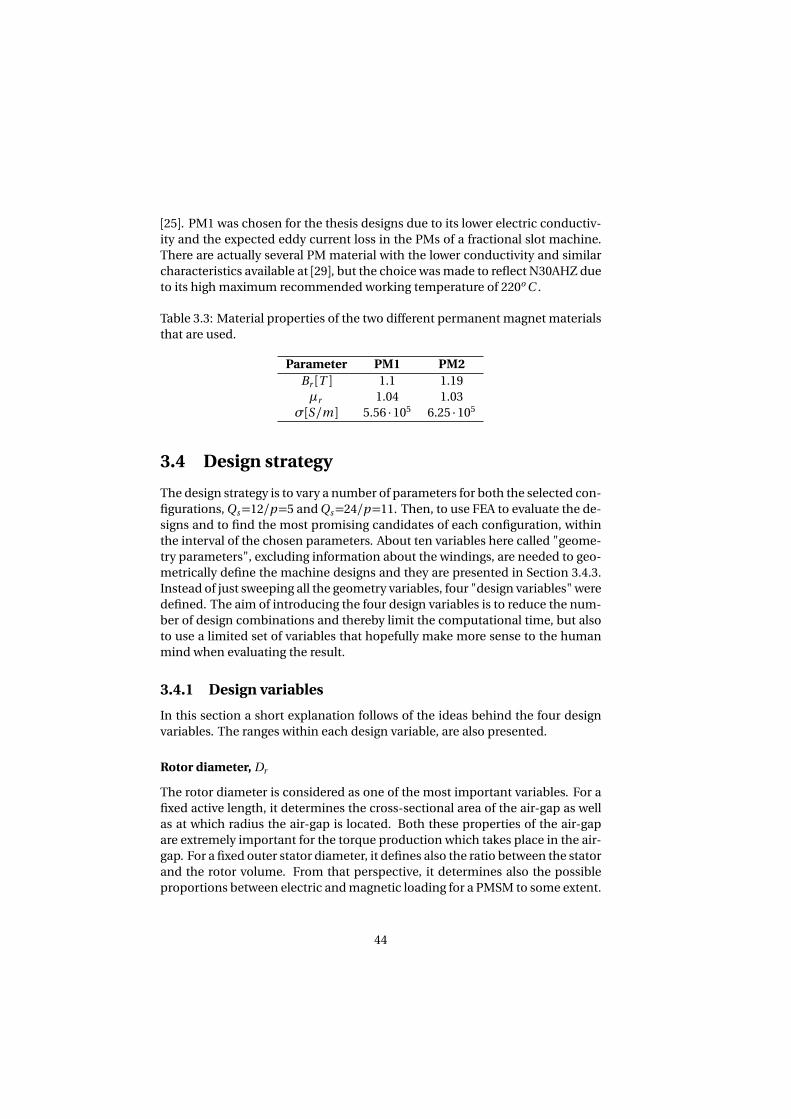
[25]. PM1 was chosen for the thesis designs due to its lower electric conductiv-

ity and the expected eddy current loss in the PMs of a fractional slot machine.

There are actually several PM material with the lower conductivity and similar

characteristics available at [29], but the choice was made to reflect N30AHZ due

to its high maximum recommended working temperature of 220o C .

Table 3.3: Material properties of the two different permanent magnet materials

that are used.

Parameter PM1 PM2

Br [T ] 1.1 1.19

µr 1.04 1.03

σ[S/m ] 5.56 ·105 6.25 ·105

3.4 Design strategy

The design strategy is to vary a number of parameters for both the selected con-

figurations, Qs=12/p=5 and Qs=24/p=11. Then, to use FEA to evaluate the de-

signs and to find the most promising candidates of each configuration, within

the interval of the chosen parameters. About ten variables here called "geome-

try parameters", excluding information about the windings, are needed to geo-

metrically define the machine designs and they are presented in Section 3.4.3.

Instead of just sweeping all the geometry variables, four "design variables" were

defined. The aim of introducing the four design variables is to reduce the num-

ber of design combinations and thereby limit the computational time, but also

to use a limited set of variables that hopefully make more sense to the human

mind when evaluating the result.

3.4.1 Design variables

In this section a short explanation follows of the ideas behind the four design

variables. The ranges within each design variable, are also presented.

Rotor diameter, Dr

The rotor diameter is considered as one of the most important variables. For a

fixed active length, it determines the cross-sectional area of the air-gap as well

as at which radius the air-gap is located. Both these properties of the air-gap

are extremely important for the torque production which takes place in the air-

gap. For a fixed outer stator diameter, it defines also the ratio between the stator

and the rotor volume. From that perspective, it determines also the possible

proportions between electric and magnetic loading for a PMSM to some extent.

44

The rotor diameter is chosen to be varied in 10 mm steps between 150 mm and

200 mm.

Air-gap length, lg

Another important variable is the air-gap length, which determines the mag-

netic coupling between the stator and the rotor. A shorter air-gap length lowers

the reluctance of the gap and increases the flux for a fixed permanent magnet

length or induced MMF-wave. This may imply that the amount of permanent

magnets and copper can be reduced. On the other hand, apart from possible

mechanical issues associated with narrow air-gaps, it gives also a more non-

linear machine. The total reluctance of the magnetic circuit will be more sen-

sitive to the non-linear reluctance of the iron path, which is relatively more sig-

nificant when compared to a low air-gap reluctance. Air-gap lengths of 0.8 mm

and 1.2 mm have been used.

Stator flux density, Bma x

The flux density level is an important aspect, why a stator flux density variable,

Bma x , is defined. Bma x is the maximal average permanent magnet flux density

over the cross-sectional area along a flux path. The aim is to design a stator

structure with a constant flux density along the flux path following the philos-

ophy presented in Section 1.3. Parts where the flux path is well defined, such

as the yoke, can be calculated easily while parts where the flux path is not well

defined, such as the shoe of the teeth, is not that straightforward. One lighter

and one heavier stator structure is designed, corresponding to stator flux levels

of 1.5 T and 1.3 T respectively. As two flux levels for the same magnetic loading

is used, the combination of PM and induced flux is altered which was discussed

in Section 1.1.

Air-gap flux density, B1

Air-gap flux density, B1, corresponds directly to the magnetic loading and is not

expected to require any further explanation. Peak flux densities of 0.85 T and

1 T are used.

45

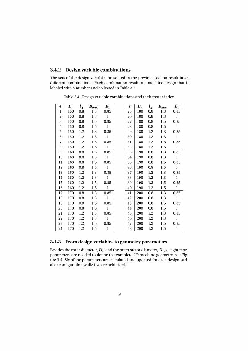
3.4.2 Design variable combinations

The sets of the design variables presented in the previous section result in 48

different combinations. Each combination result in a machine design that is

labeled with a number and collected in Table 3.4.

Table 3.4: Design variable combinations and their motor index.

# Dr l g Bm a x B1 # Dr l g Bm a x B1

1 150 0.8 1.3 0.85 25 180 0.8 1.3 0.85

2 150 0.8 1.3 1 26 180 0.8 1.3 1

3 150 0.8 1.5 0.85 27 180 0.8 1.5 0.85

4 150 0.8 1.5 1 28 180 0.8 1.5 1

5 150 1.2 1.3 0.85 29 180 1.2 1.3 0.85

6 150 1.2 1.3 1 30 180 1.2 1.3 1

7 150 1.2 1.5 0.85 31 180 1.2 1.5 0.85

8 150 1.2 1.5 1 32 180 1.2 1.5 1

9 160 0.8 1.3 0.85 33 190 0.8 1.3 0.85

10 160 0.8 1.3 1 34 190 0.8 1.3 1

11 160 0.8 1.5 0.85 35 190 0.8 1.5 0.85

12 160 0.8 1.5 1 36 190 0.8 1.5 1

13 160 1.2 1.3 0.85 37 190 1.2 1.3 0.85

14 160 1.2 1.3 1 38 190 1.2 1.3 1

15 160 1.2 1.5 0.85 39 190 1.2 1.5 0.85

16 160 1.2 1.5 1 40 190 1.2 1.5 1

17 170 0.8 1.3 0.85 41 200 0.8 1.3 0.85

18 170 0.8 1.3 1 42 200 0.8 1.3 1

19 170 0.8 1.5 0.85 43 200 0.8 1.5 0.85

20 170 0.8 1.5 1 44 200 0.8 1.5 1

21 170 1.2 1.3 0.85 45 200 1.2 1.3 0.85

22 170 1.2 1.3 1 46 200 1.2 1.3 1

23 170 1.2 1.5 0.85 47 200 1.2 1.5 0.85

24 170 1.2 1.5 1 48 200 1.2 1.5 1

3.4.3 From design variables to geometry parameters

Besides the rotor diameter, Dr , and the outer stator diameter, Do u t , eight more

parameters are needed to define the complete 2D machine geometry, see Fig-

ure 3.5. Six of the parameters are calculated and updated for each design vari-

able configuration while five are held fixed.

46

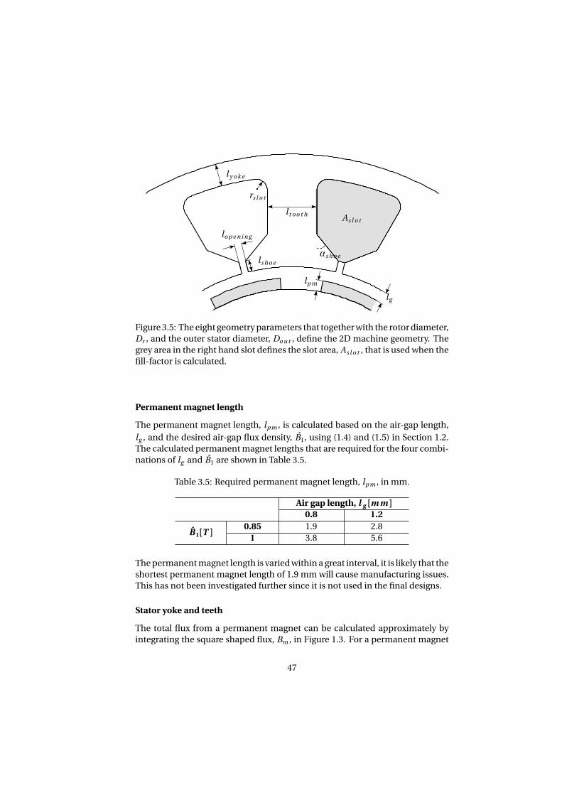
lg

lo p e ni ng

ls ho e

αs ho e

rs l o t

lt o o t h

l y o k e

lp m

As l o t

Figure 3.5: The eight geometry parameters that together with the rotor diameter,

Dr , and the outer stator diameter, Do u t , define the 2D machine geometry. The

grey area in the right hand slot defines the slot area, As l o t , that is used when the

fill-factor is calculated.

Permanent magnet length

The permanent magnet length, lp m , is calculated based on the air-gap length,

lg , and the desired air-gap flux density, B1, using (1.4) and (1.5) in Section 1.2.

The calculated permanent magnet lengths that are required for the four combi-

nations of lg and B1 are shown in Table 3.5.

Table 3.5: Required permanent magnet length, lp m , in mm.

Air gap length, l g [m m ]

0.8 1.2

B1[T ]0.85 1.9 2.8

1 3.8 5.6

The permanent magnet length is varied within a great interval, it is likely that the

shortest permanent magnet length of 1.9 mm will cause manufacturing issues.

This has not been investigated further since it is not used in the final designs.

Stator yoke and teeth

The total flux from a permanent magnet can be calculated approximately by

integrating the square shaped flux, Bm , in Figure 1.3. For a permanent magnet

47

that covers 2/3 of a pole pitch it becomes

φm = Bm

π(Dr +2lp m )2/3

2p(3.1)

which is the maximum magnetic flux that links a tooth. The required thickness

of the tooth, lt o o t h , for a given stator flux density, Bma x , is then calculated ac-

cording to

lt o o t h =φm

Bma x

(3.2)

When the PM flux that links a tooth enter the yoke region it divides about equal

between the two paths that links the two neighboring teeth. Hence, the required

thickness of the stator yoke for the same flux density is calculated as

l y o k e =φm

2Bma x

(3.3)

Fixed parameters

The fixed parameters and the values used can be seen in Table 3.6. The assumed

values used for the parameters that have been held fixed is based on discussions

and what is commonly used in existing machines. Values are therefore open for

modifications if the machines are to be prototyped.

Table 3.6: Geometry parameters that are not affected by the design variables

and held fixed.

Parameter value

Do u t 269 mm

rs l o t 5 mm

ls ho e 2 mm

αs ho e 45

lo p e ni ng 3 mm

48

Chapter 4

Analysis of fault-tolerant

fractional slot machine

designs

In this chapter, the 48 design variable combinations of each pole/slot combina-

tion are evaluated in order to motivate a choice from each set of combinations.

An appropriate number of turns are selected for the windings of the machines

and the impact of phase current on winding temperature rise is analyzed. The

two final machine designs are compared together with the Toyota Prius from

2004 in therms of performance and material cost. Some key figures from the

comparison of the three machines are summarized in the end of this chapter.

4.1 Machine design selection

The 48 machines are evaluated by comparing their torque production in rela-

tion to the material cost, [Nm/USD]. The material market price have fluctuated

substantially over the last years, especially for neodymium which today is back

on the same price levels as in 2010 (≈100 USD/kg) from the peak during 2011

(≈500 USD/kg). Due to the variation of the material cost, the current material

cost is estimated and the results are presented to take cost variation of each ma-

terial into account.

4.1.1 Estimation of the current material costs

Accurate calculations of the material costs is a difficult or even impossible task,

since the material prices varies substantially over time as mentioned previously.

Also the price at two different markets may not be the same at the same time.

49

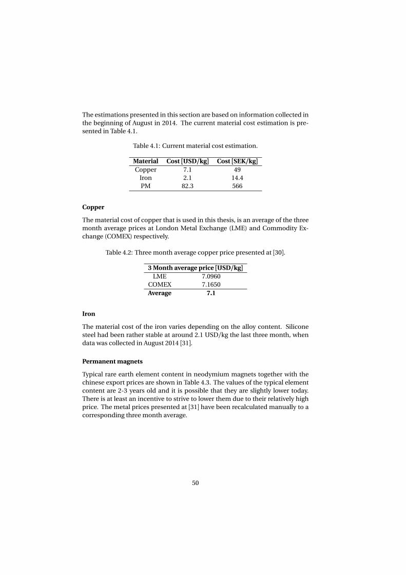
The estimations presented in this section are based on information collected in

the beginning of August in 2014. The current material cost estimation is pre-

sented in Table 4.1.

Table 4.1: Current material cost estimation.

Material Cost [USD/kg] Cost [SEK/kg]

Copper 7.1 49

Iron 2.1 14.4

PM 82.3 566

Copper

The material cost of copper that is used in this thesis, is an average of the three

month average prices at London Metal Exchange (LME) and Commodity Ex-

change (COMEX) respectively.

Table 4.2: Three month average copper price presented at [30].

3 Month average price [USD/kg]

LME 7.0960

COMEX 7.1650

Average 7.1

Iron

The material cost of the iron varies depending on the alloy content. Silicone

steel had been rather stable at around 2.1 USD/kg the last three month, when

data was collected in August 2014 [31].

Permanent magnets

Typical rare earth element content in neodymium magnets together with the

chinese export prices are shown in Table 4.3. The values of the typical element

content are 2-3 years old and it is possible that they are slightly lower today.

There is at least an incentive to strive to lower them due to their relatively high

price. The metal prices presented at [31] have been recalculated manually to a

corresponding three month average.

50

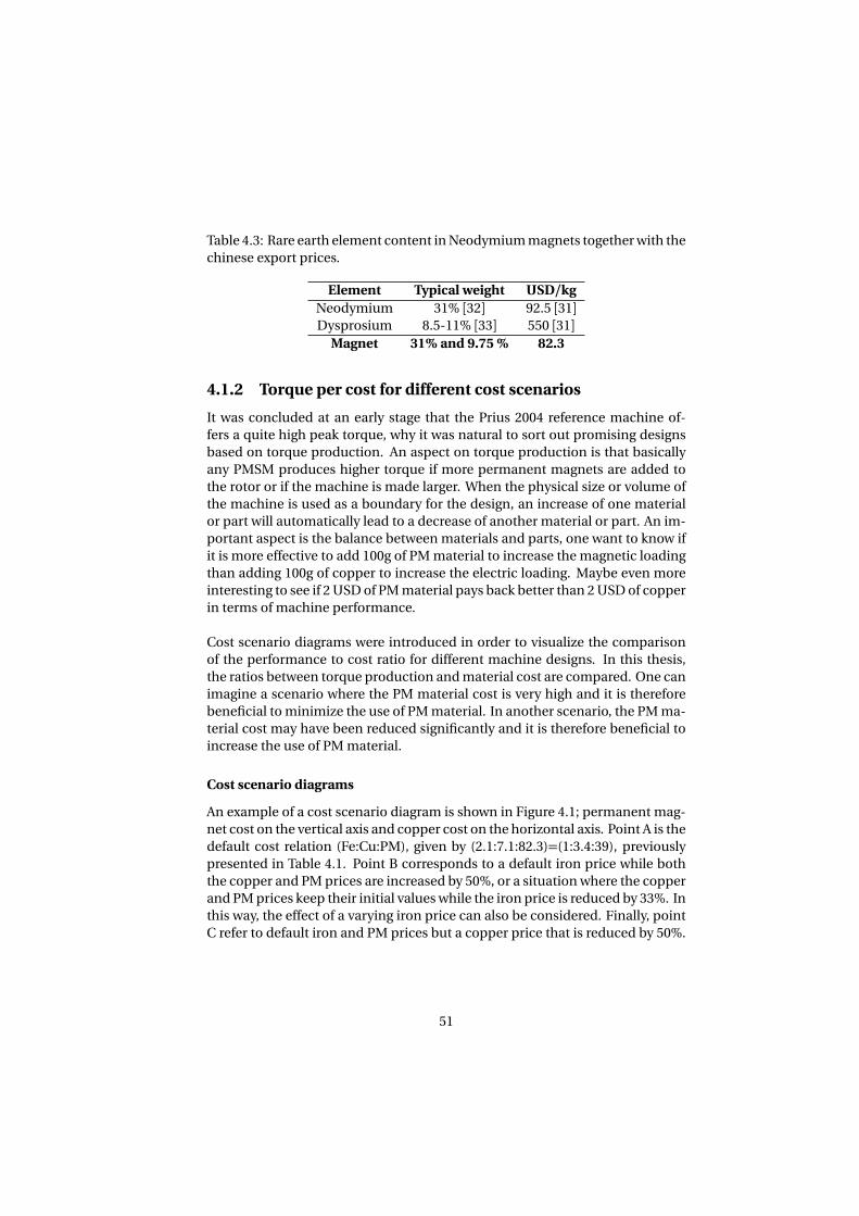
Table 4.3: Rare earth element content in Neodymium magnets together with the

chinese export prices.

Element Typical weight USD/kg

Neodymium 31% [32] 92.5 [31]

Dysprosium 8.5-11% [33] 550 [31]

Magnet 31% and 9.75 % 82.3

4.1.2 Torque per cost for different cost scenarios

It was concluded at an early stage that the Prius 2004 reference machine of-

fers a quite high peak torque, why it was natural to sort out promising designs

based on torque production. An aspect on torque production is that basically

any PMSM produces higher torque if more permanent magnets are added to

the rotor or if the machine is made larger. When the physical size or volume of

the machine is used as a boundary for the design, an increase of one material

or part will automatically lead to a decrease of another material or part. An im-

portant aspect is the balance between materials and parts, one want to know if

it is more effective to add 100g of PM material to increase the magnetic loading

than adding 100g of copper to increase the electric loading. Maybe even more

interesting to see if 2 USD of PM material pays back better than 2 USD of copper

in terms of machine performance.

Cost scenario diagrams were introduced in order to visualize the comparison

of the performance to cost ratio for different machine designs. In this thesis,

the ratios between torque production and material cost are compared. One can

imagine a scenario where the PM material cost is very high and it is therefore

beneficial to minimize the use of PM material. In another scenario, the PM ma-

terial cost may have been reduced significantly and it is therefore beneficial to

increase the use of PM material.

Cost scenario diagrams

An example of a cost scenario diagram is shown in Figure 4.1; permanent mag-

net cost on the vertical axis and copper cost on the horizontal axis. Point A is the

default cost relation (Fe:Cu:PM), given by (2.1:7.1:82.3)=(1:3.4:39), previously

presented in Table 4.1. Point B corresponds to a default iron price while both

the copper and PM prices are increased by 50%, or a situation where the copper

and PM prices keep their initial values while the iron price is reduced by 33%. In

this way, the effect of a varying iron price can also be considered. Finally, point

C refer to default iron and PM prices but a copper price that is reduced by 50%.

51

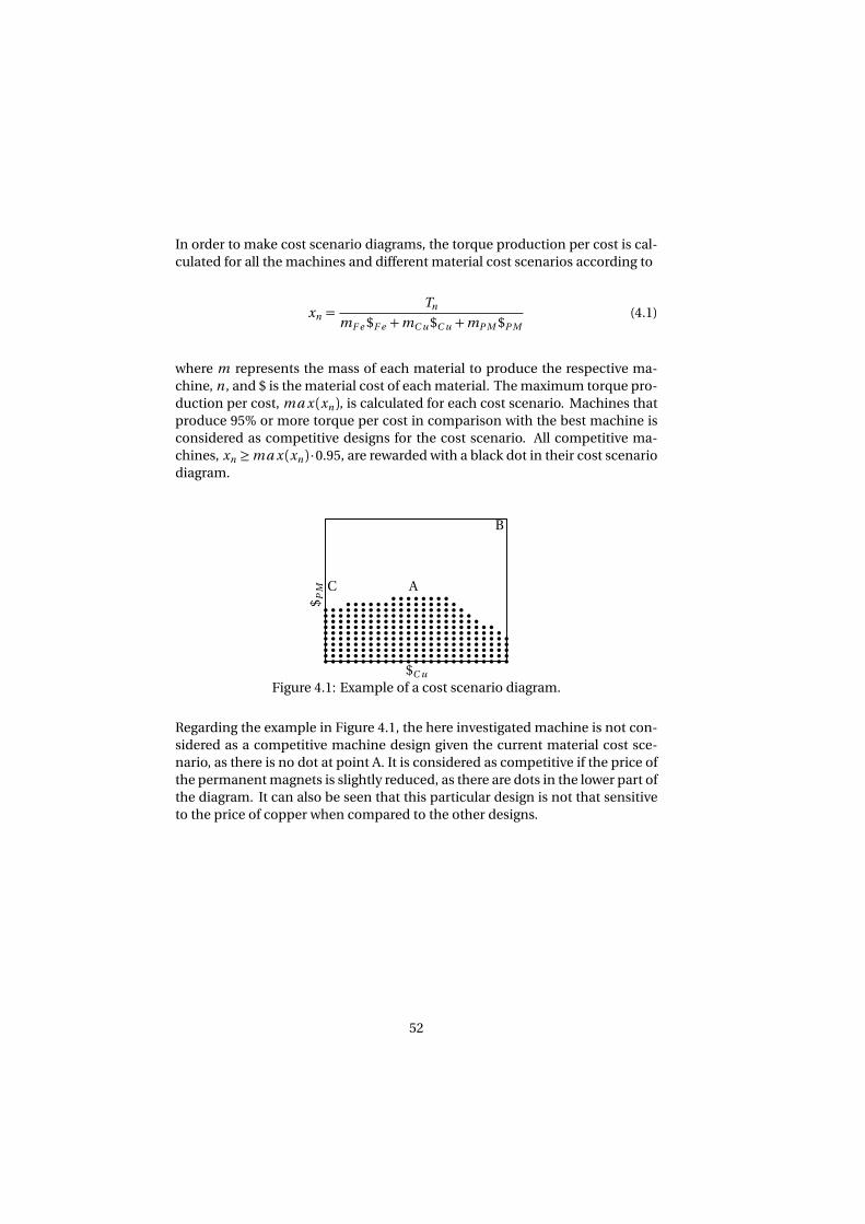
In order to make cost scenario diagrams, the torque production per cost is cal-

culated for all the machines and different material cost scenarios according to

xn =Tn

mF e $F e +mC u $C u +mP M $P M

(4.1)

where m represents the mass of each material to produce the respective ma-

chine, n , and $ is the material cost of each material. The maximum torque pro-

duction per cost, ma x (xn ), is calculated for each cost scenario. Machines that

produce 95% or more torque per cost in comparison with the best machine is

considered as competitive designs for the cost scenario. All competitive ma-

chines, xn ≥ma x (xn ) ·0.95, are rewarded with a black dot in their cost scenario

diagram.

A

B

C

$C u

$P

M

Figure 4.1: Example of a cost scenario diagram.

Regarding the example in Figure 4.1, the here investigated machine is not con-

sidered as a competitive machine design given the current material cost sce-

nario, as there is no dot at point A. It is considered as competitive if the price of

the permanent magnets is slightly reduced, as there are dots in the lower part of

the diagram. It can also be seen that this particular design is not that sensitive

to the price of copper when compared to the other designs.

52

4.1.3 Cost efficiency of the 12/5 machine designs

The output torque has been calculated at a speed of 1500 rpm for five different

excitation levels, J = [5 10 15 20] A/mm 2, in the direction of the quadrature axis

(id = 0). This to see the non-linear behavior of the machines and not to com-

pare them in just one operating point.

The cost scenario diagrams for the 48 machine designs, previously presented in

Table 3.4, excited by 5 A/mm 2 are shown in Table 4.4. It can be seen that the

most cost competitive machines have a rotor diameter of 150-160 mm, and an

air-gap of 0.8 mm. The maximal average permanent magnet flux density level,

Bma x , is not that critical at this relatively low current levels. It is clear that an

air-gap flux density, B1, of 1 T is preferable compared to 0.85 T. Machine 2, 4 and

12 are the most cost competitive at the estimated current material cost scenario.

Table 4.4: Cost scenario diagram for the 48 Qs=12/p=5 machine designs at an

excitation level of 5 A/mm 2.

l g =0.8 l g =1.2

B1

0.85 1 0.85 1 0.85 1 0.85 1

1501 2 3 4 5 6 7 8

1609 10 11 12 13 14 15 16

17017 18 19 20 21 22 23 24

Dr

18025 26 27 28 29 30 31 32

19033 34 35 36 37 38 39 40

20041 42 43 44 45 46 47 48

1.3 1.5 1.3 1.5

Bm a x

53

Table 4.5 shows cost scenario diagrams when the current excitation is 10A/mm 2,

twice as high as in the previous case. In this case, a maximal average permanent

magnet flux density level of 1.3 T is clearly preferable compared to 1.5 T. It can be

seen that machine number 6 is competitive at this excitation level if the price of

permanent magnets are reduced. One can also observe a shift towards greater

rotor diameters.

Table 4.5: Cost scenario diagram for the 48 Qs=12/p=5 machine designs at an

excitation level of 10 A/mm 2.

l g =0.8 l g =1.2

B1

0.85 1 0.85 1 0.85 1 0.85 1

1501 2 3 4 5 6 7 8

1609 10 11 12 13 14 15 16

17017 18 19 20 21 22 23 24

Dr

18025 26 27 28 29 30 31 32

19033 34 35 36 37 38 39 40

20041 42 43 44 45 46 47 48

1.3 1.5 1.3 1.5

Bm a x

54

When increasing the current density 5A/mm 2 further, the same but magnified

tendencies are shown as before. The design variables of the air-gap and stator

flux densities are at the same level for all the competitive machines. An air-gap

length of 1.2 mm is still not beneficial considering the current cost scenario, but

it will be by machine number 6 and 14 if the PM cost is lowered slightly.

Table 4.6: Cost scenario diagram for the 48 Qs=12/p=5 machine designs at an

excitation level of 15 A/mm 2.

l g =0.8 l g =1.2

B1

0.85 1 0.85 1 0.85 1 0.85 1

1501 2 3 4 5 6 7 8

1609 10 11 12 13 14 15 16

17017 18 19 20 21 22 23 24

Dr

18025 26 27 28 29 30 31 32

19033 34 35 36 37 38 39 40

20041 42 43 44 45 46 47 48

1.3 1.5 1.3 1.5

Bm a x

55

As a last step, the current density is increased up to 20 A/mm 2, and the result is

shown in Table 4.7. It can be seen that there is one machine design, number 14,

that benefits from an increased air-gap length of, lg = 1.2 mm, at this relatively

high excitation level.

Table 4.7: Cost scenario diagram for the 48 Qs=12/p=5 machine designs at an

excitation level of 20 A/mm 2.

l g =0.8 l g =1.2

B1

0.85 1 0.85 1 0.85 1 0.85 1

1501 2 3 4 5 6 7 8

1609 10 11 12 13 14 15 16

17017 18 19 20 21 22 23 24

Dr

18025 26 27 28 29 30 31 32

19033 34 35 36 37 38 39 40

20041 42 43 44 45 46 47 48

1.3 1.5 1.3 1.5

Bm a x

Based on the overall cost efficiency, considering all the four excitations levels,

machine design number 10 turned out to be a favorable choice. Machine num-

ber 10 is therefore highlighted when the 12/5 machine designs are evaluated

further.

56

4.1.4 Cost efficiency of the 24/11 machine designs

The cost scenario diagrams for theQs=24/p=11 machine designs have been cal-

culated in exactly the same manner as in the previous section. The 48 designs,

excited by 5 A/mm 2 are shown in Table 4.8. It can be seen that more machines

turned out to be cost effective if comparing with the same excitation level for

the Qs=12/p=5 machine designs in Table 4.4. There are also several machines

with lower air-gap flux density, B1=0.85 T, that are competitive at this relatively

low current level. It can also be seen that there is a general shift towards higher

rotor diameters compared with the Qs=12/p=5 machine designs. This can be

explained by the thinner stator diameter that is required when the number of

poles are increased.

Table 4.8: Cost scenario diagram for the 48 Qs=24/p=11 machine designs at an

excitation level of 5 A/mm 2.

l g =0.8 l g =1.2

B1

0.85 1 0.85 1 0.85 1 0.85 1

1501 2 3 4 5 6 7 8

1609 10 11 12 13 14 15 16

17017 18 19 20 21 22 23 24

Dr

18025 26 27 28 29 30 31 32

19033 34 35 36 37 38 39 40

20041 42 43 44 45 46 47 48

1.3 1.5 1.3 1.5

Bm a x

57

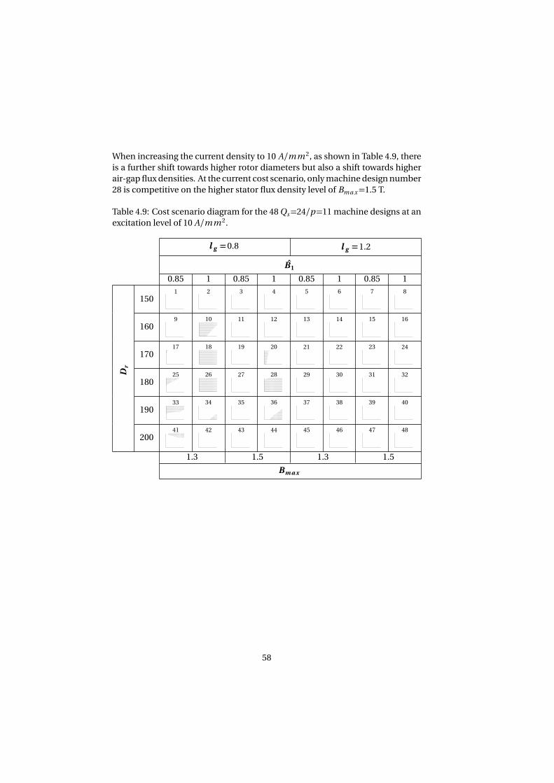
When increasing the current density to 10 A/mm 2, as shown in Table 4.9, there

is a further shift towards higher rotor diameters but also a shift towards higher

air-gap flux densities. At the current cost scenario, only machine design number

28 is competitive on the higher stator flux density level of Bma x=1.5 T.

Table 4.9: Cost scenario diagram for the 48 Qs=24/p=11 machine designs at an

excitation level of 10 A/mm 2.

l g =0.8 l g =1.2

B1

0.85 1 0.85 1 0.85 1 0.85 1

1501 2 3 4 5 6 7 8

1609 10 11 12 13 14 15 16

17017 18 19 20 21 22 23 24

Dr

18025 26 27 28 29 30 31 32

19033 34 35 36 37 38 39 40

20041 42 43 44 45 46 47 48

1.3 1.5 1.3 1.5

Bm a x

58

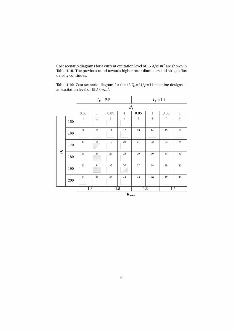
Cost scenario diagrams for a current excitation level of 15 A/mm 2 are shown in

Table 4.10. The previous trend towards higher rotor diameters and air-gap flux

density continues.

Table 4.10: Cost scenario diagram for the 48 Qs=24/p=11 machine designs at

an excitation level of 15 A/mm 2.

l g =0.8 l g =1.2

B1

0.85 1 0.85 1 0.85 1 0.85 1

1501 2 3 4 5 6 7 8

1609 10 11 12 13 14 15 16

17017 18 19 20 21 22 23 24

Dr

18025 26 27 28 29 30 31 32

19033 34 35 36 37 38 39 40

20041 42 43 44 45 46 47 48

1.3 1.5 1.3 1.5

Bm a x

59

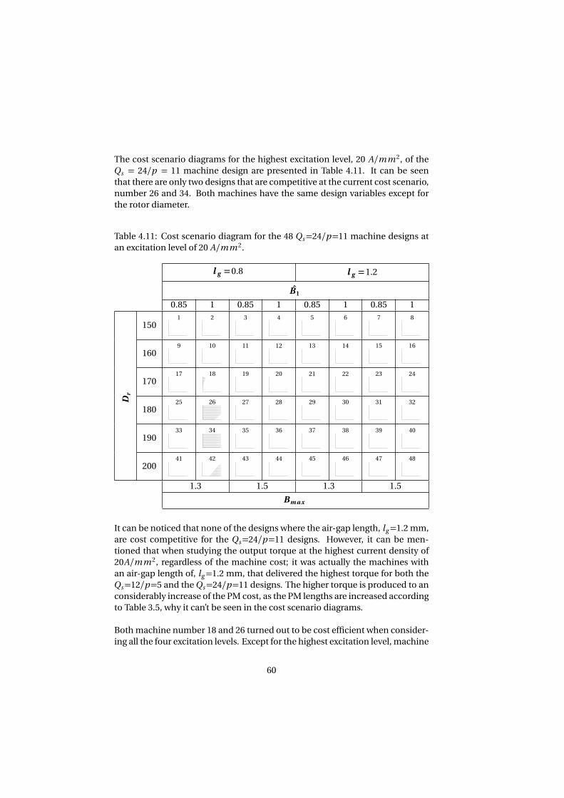
The cost scenario diagrams for the highest excitation level, 20 A/mm 2, of the

Qs = 24/p = 11 machine design are presented in Table 4.11. It can be seen

that there are only two designs that are competitive at the current cost scenario,

number 26 and 34. Both machines have the same design variables except for

the rotor diameter.

Table 4.11: Cost scenario diagram for the 48 Qs=24/p=11 machine designs at

an excitation level of 20 A/mm 2.

l g =0.8 l g =1.2

B1

0.85 1 0.85 1 0.85 1 0.85 1

1501 2 3 4 5 6 7 8

1609 10 11 12 13 14 15 16

17017 18 19 20 21 22 23 24

Dr

18025 26 27 28 29 30 31 32

19033 34 35 36 37 38 39 40

20041 42 43 44 45 46 47 48

1.3 1.5 1.3 1.5

Bm a x

It can be noticed that none of the designs where the air-gap length, lg=1.2 mm,

are cost competitive for the Qs=24/p=11 designs. However, it can be men-

tioned that when studying the output torque at the highest current density of

20A/mm 2, regardless of the machine cost; it was actually the machines with

an air-gap length of, lg=1.2 mm, that delivered the highest torque for both the

Qs=12/p=5 and the Qs=24/p=11 designs. The higher torque is produced to an

considerably increase of the PM cost, as the PM lengths are increased according

to Table 3.5, why it can’t be seen in the cost scenario diagrams.

Both machine number 18 and 26 turned out to be cost efficient when consider-

ing all the four excitation levels. Except for the highest excitation level, machine

60

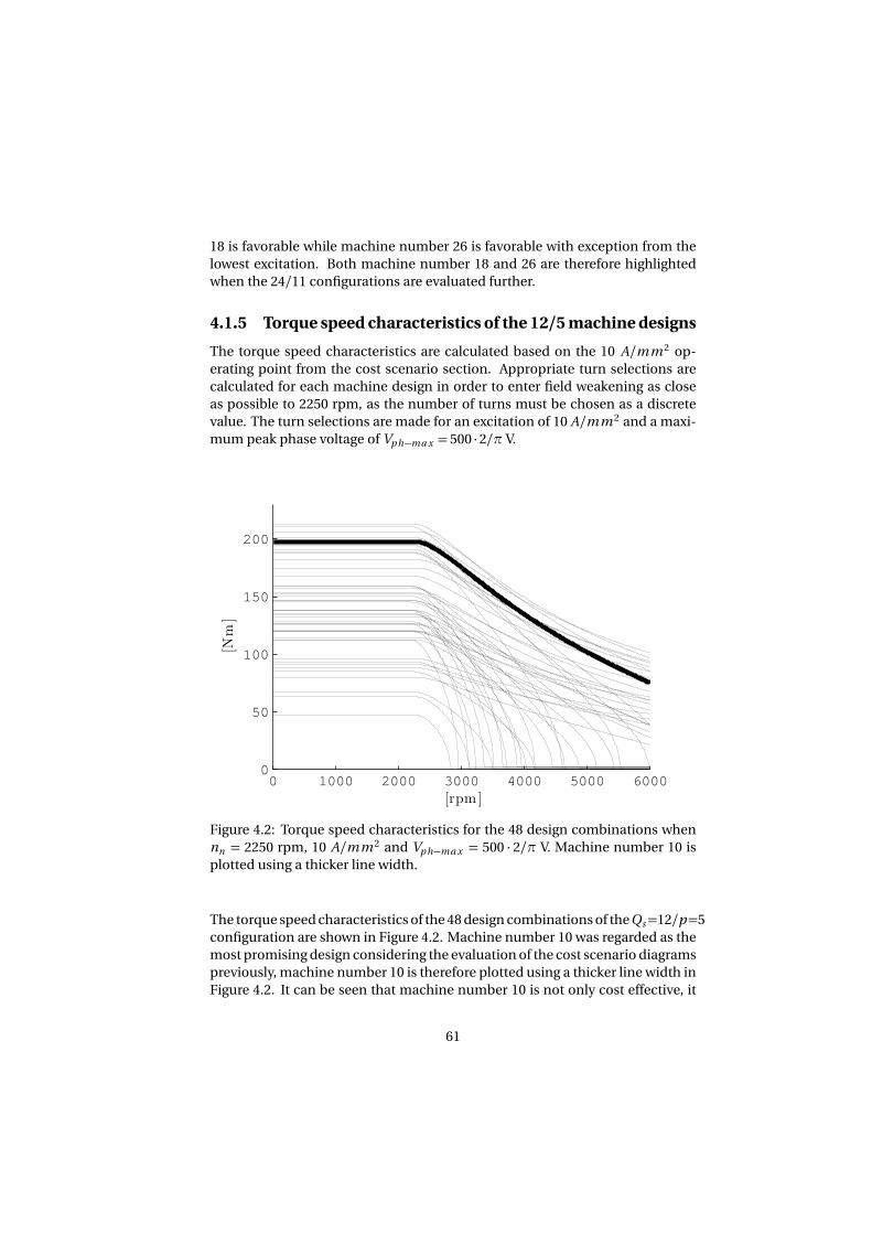
18 is favorable while machine number 26 is favorable with exception from the

lowest excitation. Both machine number 18 and 26 are therefore highlighted

when the 24/11 configurations are evaluated further.

4.1.5 Torque speed characteristics of the 12/5 machine designs

The torque speed characteristics are calculated based on the 10 A/mm 2 op-

erating point from the cost scenario section. Appropriate turn selections are

calculated for each machine design in order to enter field weakening as close

as possible to 2250 rpm, as the number of turns must be chosen as a discrete

value. The turn selections are made for an excitation of 10 A/mm 2 and a maxi-

mum peak phase voltage of Vp h−ma x = 500 ·2/π V.

0 1000 2000 3000 4000 5000 60000

50

100

150

200

[Nm]

[rpm ]

Figure 4.2: Torque speed characteristics for the 48 design combinations when

nn = 2250 rpm, 10 A/mm 2 and Vp h−ma x = 500 · 2/π V. Machine number 10 is

plotted using a thicker line width.

The torque speed characteristics of the 48 design combinations of theQs=12/p=5

configuration are shown in Figure 4.2. Machine number 10 was regarded as the

most promising design considering the evaluation of the cost scenario diagrams

previously, machine number 10 is therefore plotted using a thicker line width in

Figure 4.2. It can be seen that machine number 10 is not only cost effective, it

61

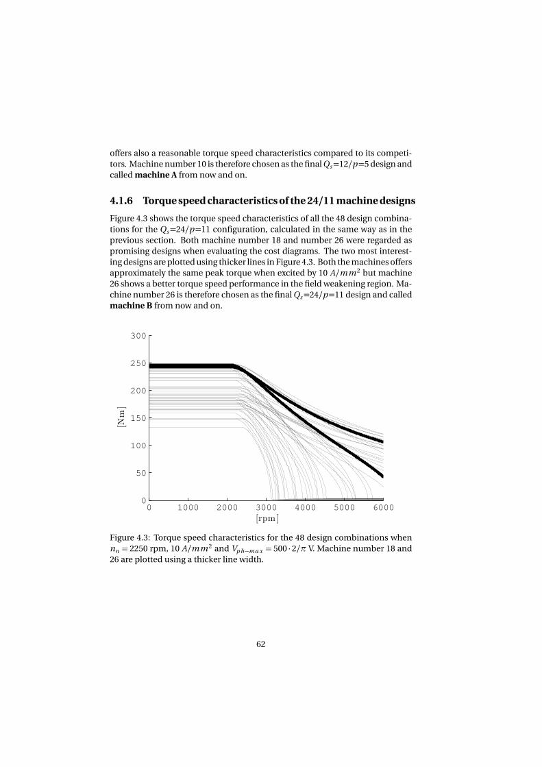
offers also a reasonable torque speed characteristics compared to its competi-

tors. Machine number 10 is therefore chosen as the final Qs=12/p=5 design and

called machine A from now and on.

4.1.6 Torque speed characteristics of the 24/11 machine designs

Figure 4.3 shows the torque speed characteristics of all the 48 design combina-

tions for the Qs=24/p=11 configuration, calculated in the same way as in the

previous section. Both machine number 18 and number 26 were regarded as

promising designs when evaluating the cost diagrams. The two most interest-

ing designs are plotted using thicker lines in Figure 4.3. Both the machines offers

approximately the same peak torque when excited by 10 A/mm 2 but machine

26 shows a better torque speed performance in the field weakening region. Ma-

chine number 26 is therefore chosen as the final Qs=24/p=11 design and called

machine B from now and on.

0 1000 2000 3000 4000 5000 60000

50

100

150

200

250

300

[Nm]

[rpm ]

Figure 4.3: Torque speed characteristics for the 48 design combinations when

nn = 2250 rpm, 10 A/mm 2 and Vp h−ma x = 500 · 2/π V. Machine number 18 and

26 are plotted using a thicker line width.

62

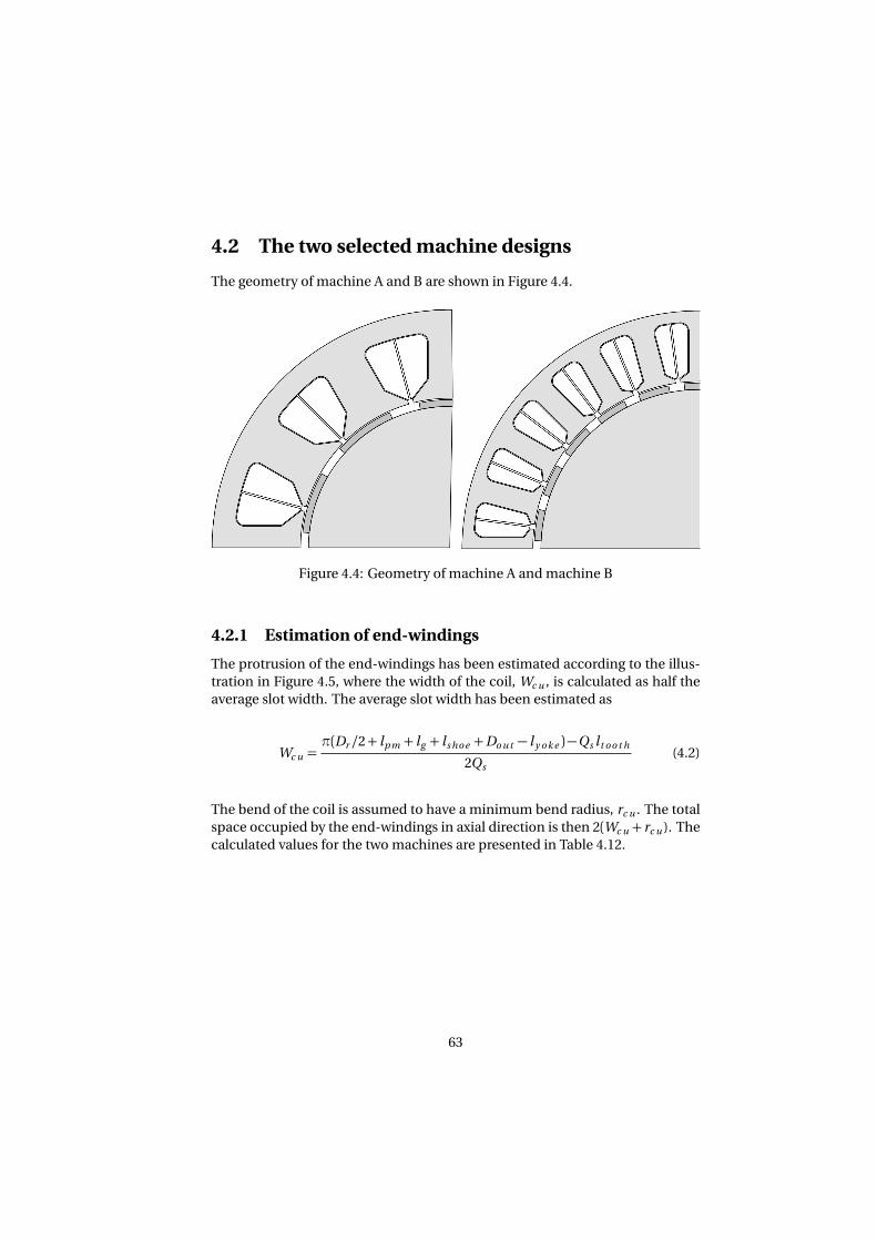
4.2 The two selected machine designs

The geometry of machine A and B are shown in Figure 4.4.

Figure 4.4: Geometry of machine A and machine B

4.2.1 Estimation of end-windings

The protrusion of the end-windings has been estimated according to the illus-

tration in Figure 4.5, where the width of the coil, Wc u , is calculated as half the

average slot width. The average slot width has been estimated as

Wc u =π(Dr /2+ lp m + lg + ls ho e +Do u t − l y o k e )−Qs lt o o t h

2Qs

(4.2)

The bend of the coil is assumed to have a minimum bend radius, rc u . The total

space occupied by the end-windings in axial direction is then 2(Wc u + rc u ). The

calculated values for the two machines are presented in Table 4.12.

63

wc u

wc u

rc u

Figure 4.5: Illustration of how the axial protrusion of the end-windings have

been estimated.

No measured values of the total length (stator stack+ end-windings) of the Prius

2004 machine was found. However, using the known stack length of 84 mm

and a photograph presented in [34], the total length was estimated to be around

140 mm. According to [35], the end-windings or the "coil-end length" of the

Toyota Prius 2010 machine are 29 mm each. In [24] it is shown that the winding

configuration of the 2004 and the 2010 Prius machines are not identical but sim-

ilar. The total length of the 2004 Prius stack length in [24] and the end-windings

of the 2010 Prius in [35] is 142 mm.

If a total length of 140 mm is assumed together with the values presented in Ta-

ble 4.12, it was possible to extend the 2004 Prius stack length by 24% for machine

A and by 40% for machine B. These numbers are to be compared with the as-

sumption of 30% made in section 3.1. By adding the estimated end-windings to

the assumed stack length of 108 mm, the total stack length of machine A turned

out to be 146 mm and machine B turned out to be 132 mm. These numbers in-

dicate that machine A has been made 6 mm too long and that it is possible to

extend machine B by 8 mm additional. Because of time constraints and the un-

certainties involved in the end-winding estimation, it was decided to keep the

stator stack length according to the initial assumption of 30% extension of the

2004 Prius stator stack length.

Table 4.12: End-winding estimation using a minimum bend radius, rc u , of 3

mm.

Machine A Machine B

Wc u [mm] 15.5 8.5

2(Wc u + rc u ) [mm] 37.0 23.00

64

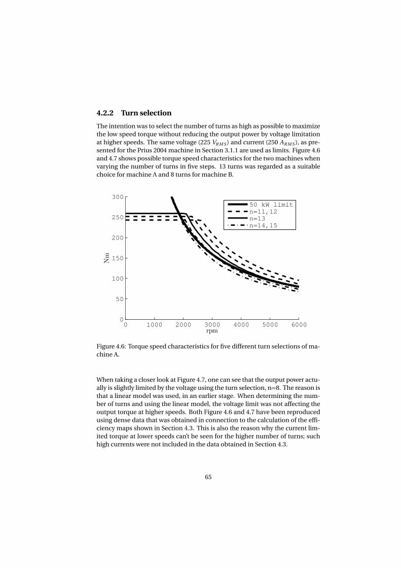
4.2.2 Turn selection

The intention was to select the number of turns as high as possible to maximize

the low speed torque without reducing the output power by voltage limitation

at higher speeds. The same voltage (225 VR M S ) and current (250 AR M S ), as pre-

sented for the Prius 2004 machine in Section 3.1.1 are used as limits. Figure 4.6

and 4.7 shows possible torque speed characteristics for the two machines when

varying the number of turns in five steps. 13 turns was regarded as a suitable

choice for machine A and 8 turns for machine B.

0 1000 2000 3000 4000 5000 60000

50

100

150

200

250

300

rpm

Nm

50 kW limitn=11,12n=13n=14,15

Figure 4.6: Torque speed characteristics for five different turn selections of ma-

chine A.

When taking a closer look at Figure 4.7, one can see that the output power actu-

ally is slightly limited by the voltage using the turn selection, n=8. The reason is

that a linear model was used, in an earlier stage. When determining the num-

ber of turns and using the linear model, the voltage limit was not affecting the

output torque at higher speeds. Both Figure 4.6 and 4.7 have been reproduced

using dense data that was obtained in connection to the calculation of the effi-

ciency maps shown in Section 4.3. This is also the reason why the current lim-

ited torque at lower speeds can’t be seen for the higher number of turns; such

high currents were not included in the data obtained in Section 4.3.

65

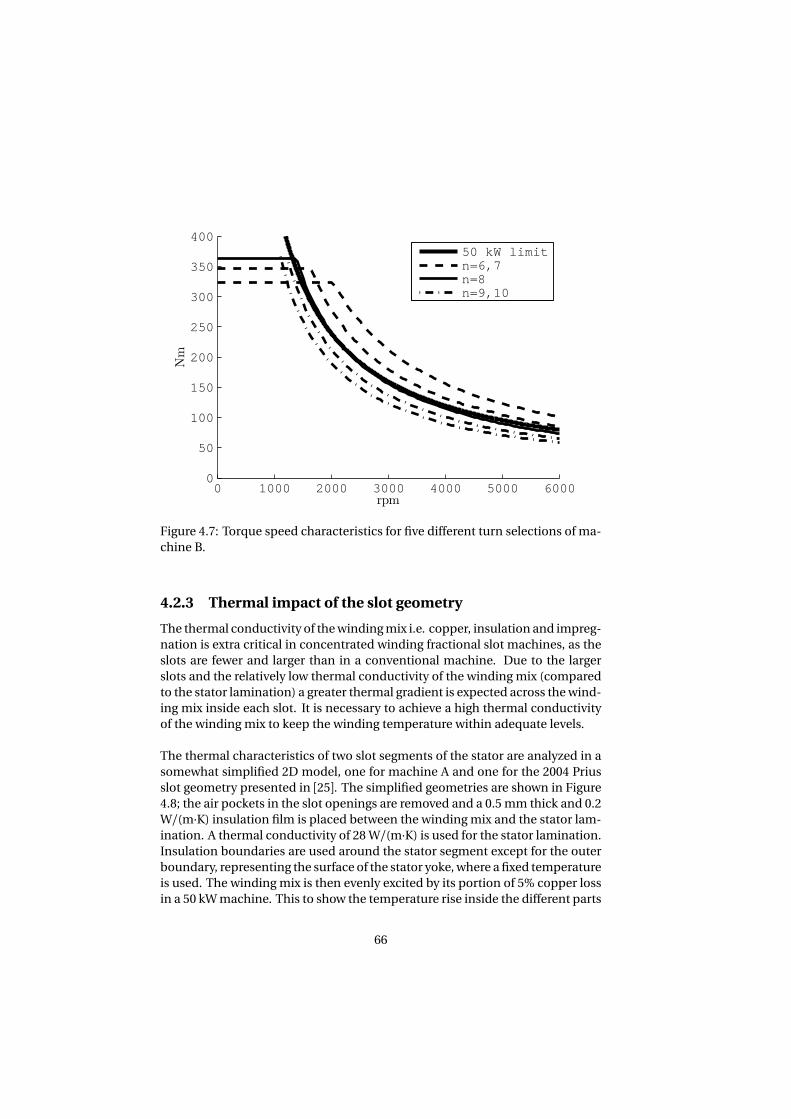
0 1000 2000 3000 4000 5000 60000

50

100

150

200

250

300

350

400

rpm

Nm

50 kW limitn=6,7n=8n=9,10

Figure 4.7: Torque speed characteristics for five different turn selections of ma-

chine B.

4.2.3 Thermal impact of the slot geometry

The thermal conductivity of the winding mix i.e. copper, insulation and impreg-

nation is extra critical in concentrated winding fractional slot machines, as the

slots are fewer and larger than in a conventional machine. Due to the larger

slots and the relatively low thermal conductivity of the winding mix (compared

to the stator lamination) a greater thermal gradient is expected across the wind-

ing mix inside each slot. It is necessary to achieve a high thermal conductivity

of the winding mix to keep the winding temperature within adequate levels.

The thermal characteristics of two slot segments of the stator are analyzed in a

somewhat simplified 2D model, one for machine A and one for the 2004 Prius

slot geometry presented in [25]. The simplified geometries are shown in Figure

4.8; the air pockets in the slot openings are removed and a 0.5 mm thick and 0.2

W/(m·K) insulation film is placed between the winding mix and the stator lam-

ination. A thermal conductivity of 28 W/(m·K) is used for the stator lamination.

Insulation boundaries are used around the stator segment except for the outer

boundary, representing the surface of the stator yoke, where a fixed temperature

is used. The winding mix is then evenly excited by its portion of 5% copper loss

in a 50 kW machine. This to show the temperature rise inside the different parts

66

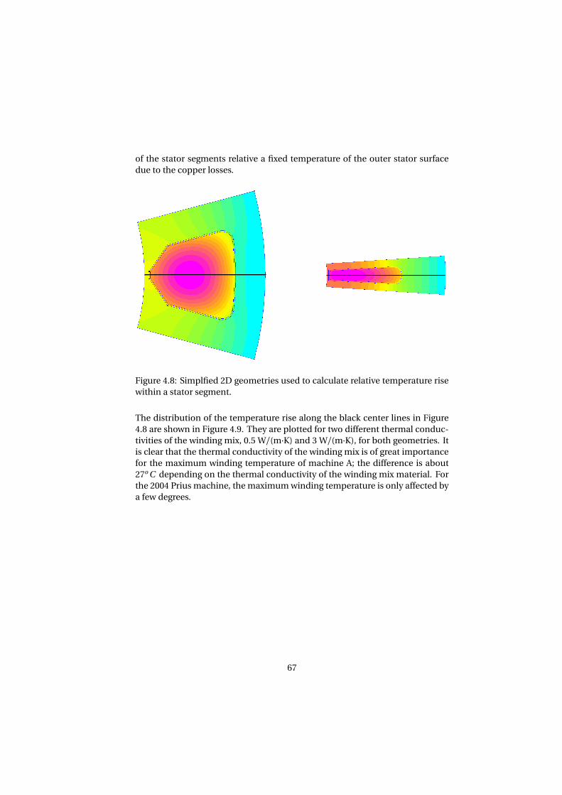
of the stator segments relative a fixed temperature of the outer stator surface

due to the copper losses.

Figure 4.8: Simplfied 2D geometries used to calculate relative temperature rise

within a stator segment.

The distribution of the temperature rise along the black center lines in Figure

4.8 are shown in Figure 4.9. They are plotted for two different thermal conduc-

tivities of the winding mix, 0.5 W/(m·K) and 3 W/(m·K), for both geometries. It

is clear that the thermal conductivity of the winding mix is of great importance

for the maximum winding temperature of machine A; the difference is about

27o C depending on the thermal conductivity of the winding mix material. For

the 2004 Prius machine, the maximum winding temperature is only affected by

a few degrees.

67

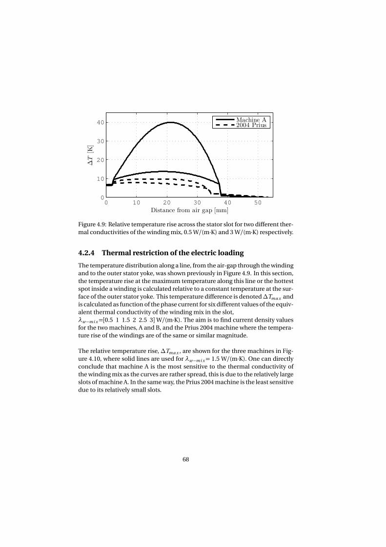
0 10 20 30 40 500

10

20

30

40

Distance from air gap [mm]

∆T

[K]

Machine A2004 Prius

Figure 4.9: Relative temperature rise across the stator slot for two different ther-

mal conductivities of the winding mix, 0.5 W/(m·K) and 3 W/(m·K) respectively.

4.2.4 Thermal restriction of the electric loading

The temperature distribution along a line, from the air-gap through the winding

and to the outer stator yoke, was shown previously in Figure 4.9. In this section,

the temperature rise at the maximum temperature along this line or the hottest

spot inside a winding is calculated relative to a constant temperature at the sur-

face of the outer stator yoke. This temperature difference is denoted∆Tma x and

is calculated as function of the phase current for six different values of the equiv-

alent thermal conductivity of the winding mix in the slot,

λw−mi x=[0.5 1 1.5 2 2.5 3]W/(m·K). The aim is to find current density values

for the two machines, A and B, and the Prius 2004 machine where the tempera-

ture rise of the windings are of the same or similar magnitude.

The relative temperature rise, ∆Tma x , are shown for the three machines in Fig-

ure 4.10, where solid lines are used for λw−mi x= 1.5 W/(m·K). One can directly

conclude that machine A is the most sensitive to the thermal conductivity of

the winding mix as the curves are rather spread, this is due to the relatively large

slots of machine A. In the same way, the Prius 2004 machine is the least sensitive

due to its relatively small slots.

68

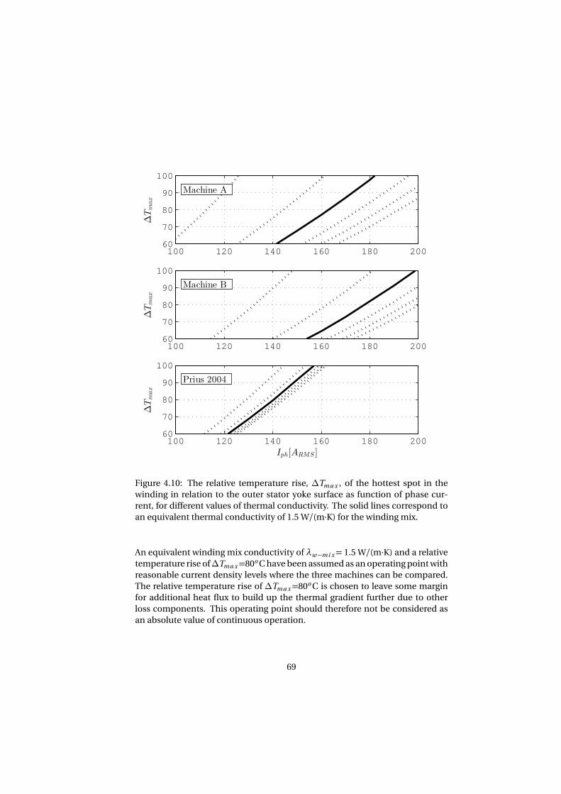
100 120 140 160 180 20060

70

80

90

100

∆Tmax

Machine A

100 120 140 160 180 20060

70

80

90

100

∆Tmax

Machine B

100 120 140 160 180 20060

70

80

90

100

Iph[ARMS ]

∆Tmax

Prius 2004

Figure 4.10: The relative temperature rise, ∆Tma x , of the hottest spot in the

winding in relation to the outer stator yoke surface as function of phase cur-

rent, for different values of thermal conductivity. The solid lines correspond to

an equivalent thermal conductivity of 1.5 W/(m·K) for the winding mix.

An equivalent winding mix conductivity of λw−mi x= 1.5 W/(m·K) and a relative

temperature rise of∆Tma x=80o C have been assumed as an operating point with

reasonable current density levels where the three machines can be compared.

The relative temperature rise of ∆Tma x=80o C is chosen to leave some margin

for additional heat flux to build up the thermal gradient further due to other

loss components. This operating point should therefore not be considered as

an absolute value of continuous operation.

69

4.3 Efficiency

Before the efficiency maps can be obtained, the operating points have to be cal-

culated. A number of transient simulations, for different iq and id combina-

tions, were carried out for each machine. The average torque as a function of

the currents, Ta v g (iq , id ), and the fundamental component of the stator flux as

a function of the currents, Ψ1s(iq , id ), were calculated. The shortest current vec-

tor, minÆ

iq + id

, that fulfills the current limit, the power limit and the voltage

limit is then calculated for each operating point.

The efficiency maps have been interpolated over 126 operating points made up

by 9 current excitation levels and 14 speed levels, represented by the black dots

in the efficiency maps. The outer black lines in the efficiency maps show the

peak torque limited by current or voltage or power. The inner black lines shows

the calculated torque limited by their respective∆Tma x=80o C current, defined

in the previous section.

Each operating point is simulated over two electrical periods where the losses

have been calculated as an average over the last period. Core losses, PF e , of

the rotors and stators are extracted directly from the FEA software together with

the eddy current losses in the PMs, PP M . Copper losses, PC u , are calculated in

a postprocess manner using phase currents and phase resistances. The Prius

2004 phase resistance of 69 mΩ at 21 o C presented in [24] has been recalculated

to 91.5 mΩ corresponding to the copper resistivity at 120 o C in Section 3.3. The

phase resistances of machine A, 20.5 mΩ, and machine B, 28.1 mΩ, are calcu-

lated including the estimations of the end-windings presented in Section 4.12

and considering the copper resistivity at 120 o C. The output power is calculated

as the average torque multiplied with the mechanical speed at each operating

point. The efficiency, η, in the efficiency map represents then

η=Ta v gΩ

Ta v gΩ+PF e +PP M +PC u

(4.3)

70

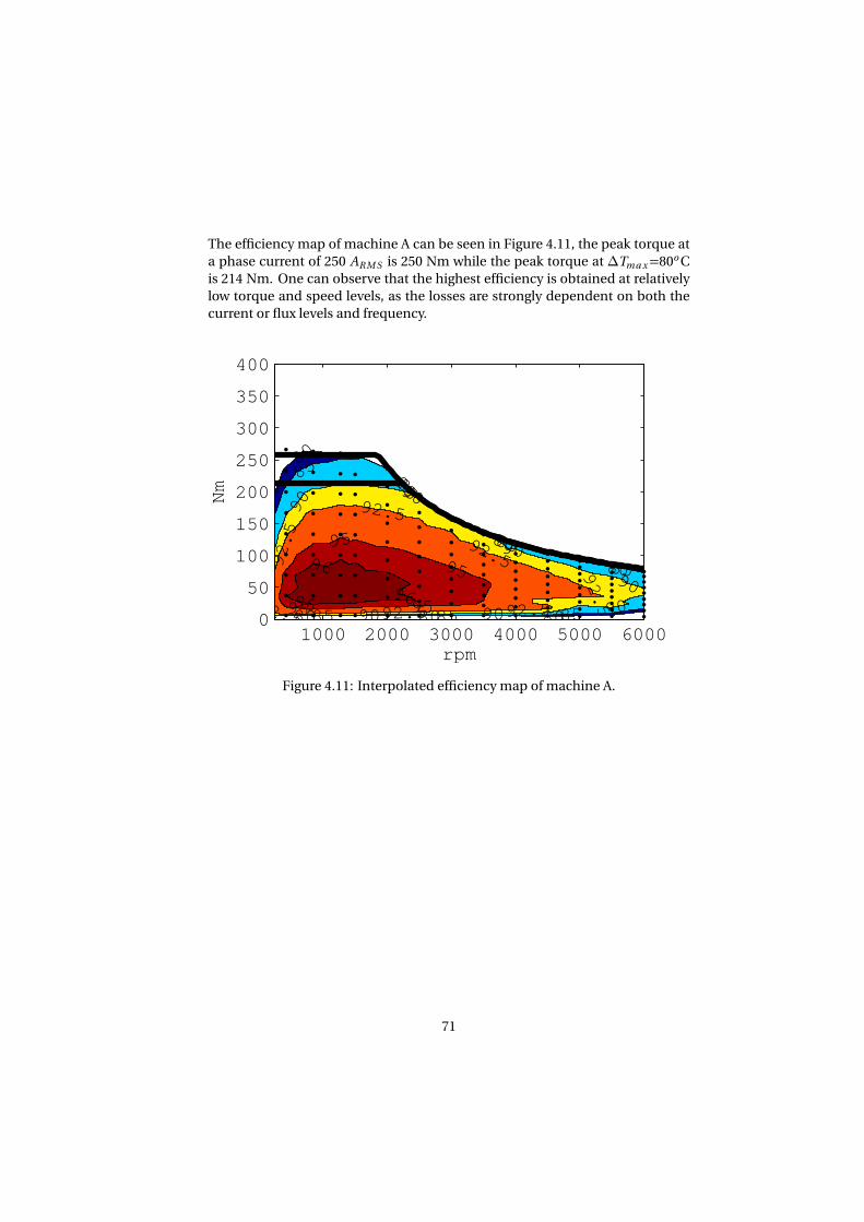
The efficiency map of machine A can be seen in Figure 4.11, the peak torque at

a phase current of 250 AR M S is 250 Nm while the peak torque at ∆Tma x=80o C

is 214 Nm. One can observe that the highest efficiency is obtained at relatively

low torque and speed levels, as the losses are strongly dependent on both the

current or flux levels and frequency.

808080

80

8080

8080

858585

85

8585

8585

909090

90

90

90

90

90

92.5

92.5

92.5

92.5

92.592.592.5

9595

9595

96

9696

rpm

Nm

1000 2000 3000 4000 5000 60000

50

100

150

200

250

300

350

400

Figure 4.11: Interpolated efficiency map of machine A.

71

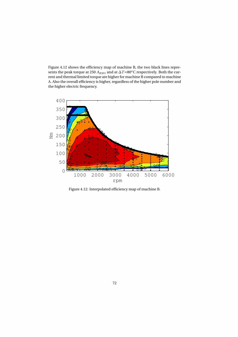
Figure 4.12 shows the efficiency map of machine B, the two black lines repre-

sents the peak torque at 250 AR M S and at∆T=80o C respectively. Both the cur-

rent and thermal limited torque are higher for machine B compared to machine

A. Also the overall efficiency is higher, regardless of the higher pole number and

the higher electric frequency.

808080

80

80

80

80

8080

858585

85

85

85

85

8585

909090

90

90

90

90

9090

92.5

92.5

92.5

92.592.5

92.592.592.5

95

95

95

959595

96

96

96

9696

97

rpm

Nm

1000 2000 3000 4000 5000 60000

50

100

150

200

250

300

350

400

Figure 4.12: Interpolated efficiency map of machine B.

72

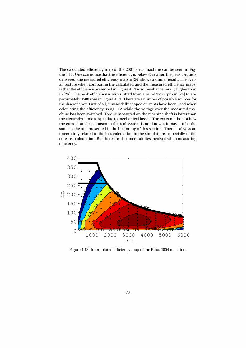
The calculated efficiency map of the 2004 Prius machine can be seen in Fig-

ure 4.13. One can notice that the efficiency is below 80% when the peak torque is

delivered, the measured efficiency map in [26] shows a similar result. The over-

all picture when comparing the calculated and the measured efficiency maps,

is that the efficiency presented in Figure 4.13 is somewhat generally higher than

in [26]. The peak efficiency is also shifted from around 2250 rpm in [26] to ap-

proximately 3500 rpm in Figure 4.13. There are a number of possible sources for

the discrepancy. First of all, sinusoidally shaped currents have been used when

calculating the efficiency using FEA while the voltage over the measured ma-

chine has been switched. Torque measured on the machine shaft is lower than

the electrodynamic torque due to mechanical losses. The exact method of how

the current angle is chosen in the real system is not known, it may not be the

same as the one presented in the beginning of this section. There is always an

uncertainty related to the loss calculation in the simulations, especially to the

core loss calculation. But there are also uncertainties involved when measuring

efficiency.

808080

80

80

80

80

8080

85858585

85

85

85

8585

909090

90

90

90

9090

92.592.592.5

92.5

92.5

92.592.5

9595

95

9595

95

9696

96

96

96

9797

97

rpm

Nm

1000 2000 3000 4000 5000 60000

50

100

150

200

250

300

350

400

Figure 4.13: Interpolated efficiency map of the Prius 2004 machine.

73

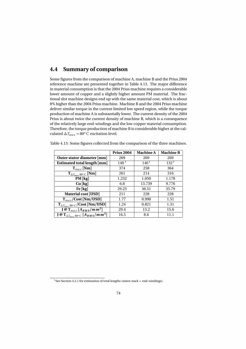
4.4 Summary of comparison

Some figures from the comparison of machine A, machine B and the Prius 2004

reference machine are presented together in Table 4.13. The major difference

in material consumption is that the 2004 Prius machine requires a considerable

lower amount of copper and a slightly higher amount PM material. The frac-

tional slot machine designs end up with the same material cost, which is about

8% higher than the 2004 Prius machine. Machine B and the 2004 Prius machine

deliver similar torque in the current limited low speed region, while the torque

production of machine A is substantially lower. The current density of the 2004

Prius is about twice the current density of machine B, which is a consequence

of the relatively large end-windings and the low copper material consumption.

Therefore, the torque production of machine B is considerable higher at the cal-

culated∆Tma x = 80o C excitation level.

Table 4.13: Some figures collected from the comparison of the three machines.

Prius 2004 Machine A Machine B

Outer stator diameter [mm] 269 269 269

Estimated total length [mm] 140 1 146 1 132 1

Tma x [Nm] 374 258 364

T∆Tma x 80o C [Nm] 261 214 316

PM [kg] 1.232 1.050 1.178

Cu [kg] 6.8 13.739 9.776

Fe [kg] 29.25 36.51 35.79

Material cost [USD] 211 228 228

Tma x /Cost [Nm/USD] 1.77 0.990 1.51

T∆Tma x 80o C /Cost [Nm/USD] 1.24 0.821 1.31

J @ Tma x [A R M S /m m 2] 29.4 13.2 15.6

J @ T∆Tma x 80o C [A R M S /m m 2] 16.5 8.6 11.1

1See Section 4.2.1 for estimation of total lengths (stator stack + end-windings).

74

Chapter 5

Per phase flux machine model

This chapter presents an alternative approach to model the PMSM during un-

balanced conditions. The relatively low mutual coupling between the phases

are simply neglected, it is thereby made relatively easy to take the individual sat-

uration levels of the different phases into account. The difference between the

flux levels of the phases might be remarkable when one phase is operated so that

its flux is enhanced while another phase is operated so that the flux is weakened.

A numerical method to calculate operating points when taking the individual

saturation levels, during unbalanced conditions, into account are presented in

the end of the chapter.

5.1 Flux representation in a single phase

The idea of the per phase flux machine model is to utilize the fact that the fault-

tolerant machine is designed to get a very low mutual coupling between the

phases. If the coupling between the phases are neglected, the flux in one phase

is just a function of the rotor position and the current in the phase itself. If the

flux and the torque in one phase is calculated as a function of the rotor position

and the current, it is possible to utilize the same 2-dimensional flux and torque

maps for all the three phases by including a phase shift of the rotor position. In

the stationary reference frame, the phase voltage can be expressed as

vp h =R ip h +dψp h

d t(5.1)

where the phase flux derivative can be divided into two parts, one that is related

to the phase current and one that is related to the rotor position

75

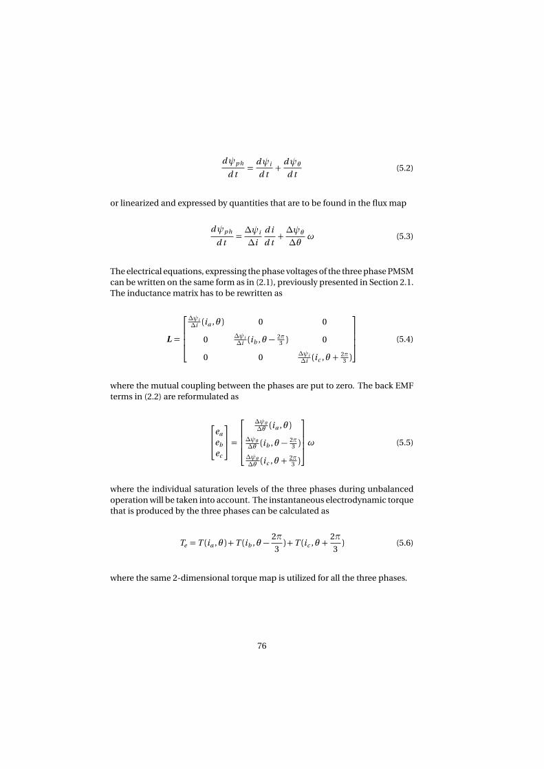
dψp h

d t=

dψi

d t+

dψθ

d t(5.2)

or linearized and expressed by quantities that are to be found in the flux map

dψp h

d t=∆ψi

∆i

d i

d t+∆ψθ

∆θω (5.3)

The electrical equations, expressing the phase voltages of the three phase PMSM

can be written on the same form as in (2.1), previously presented in Section 2.1.

The inductance matrix has to be rewritten as

L =

∆ψi

∆i (ia ,θ ) 0 0

0∆ψi

∆i (ib ,θ − 2π3 ) 0

0 0∆ψi

∆i (ic ,θ + 2π3 )

(5.4)

where the mutual coupling between the phases are put to zero. The back EMF

terms in (2.2) are reformulated as

ea

eb

ec

=

∆ψθ∆θ (ia ,θ )

∆ψθ∆θ (ib ,θ − 2π

3 )

∆ψθ∆θ (ic ,θ + 2π

3 )

ω (5.5)

where the individual saturation levels of the three phases during unbalanced

operation will be taken into account. The instantaneous electrodynamic torque

that is produced by the three phases can be calculated as

Te = T (ia ,θ ) +T (ib ,θ − 2π

3) +T (ic ,θ +

2π

3) (5.6)

where the same 2-dimensional torque map is utilized for all the three phases.

76

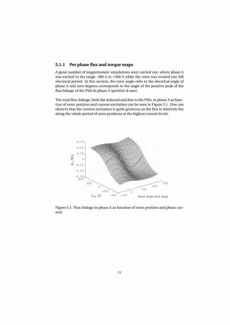
5.1.1 Per phase flux and torque maps

A great number of magnetostatic simulations were carried out, where phase A

was excited in the range -360 A to +360 A while the rotor was rotated one full

electrical period. In this section, the rotor angle refer to the electrical angle of

phase A and zero degrees corresponds to the angle of the positive peak of the

flux linkage of the PMs in phase A (positive d-axis).

The total flux-linkage, both the induced and due to the PMs, in phase A as func-

tion of rotor position and current excitation can be seen in Figure 5.1. One can

observe that the current excitation is quite generous as the flux is relatively flat

along the whole period of rotor positions at the highest current levels.

−1000

100200

300

−400

−200

0

200

400−0.03

−0.02

−0.01

0

0.01

0.02

0.03

Rotor Angle phA [degs]IphA [A]

ΨA[W

b]

Figure 5.1: Flux-linkage in phase A as function of rotor position and phase cur-

rent.

77

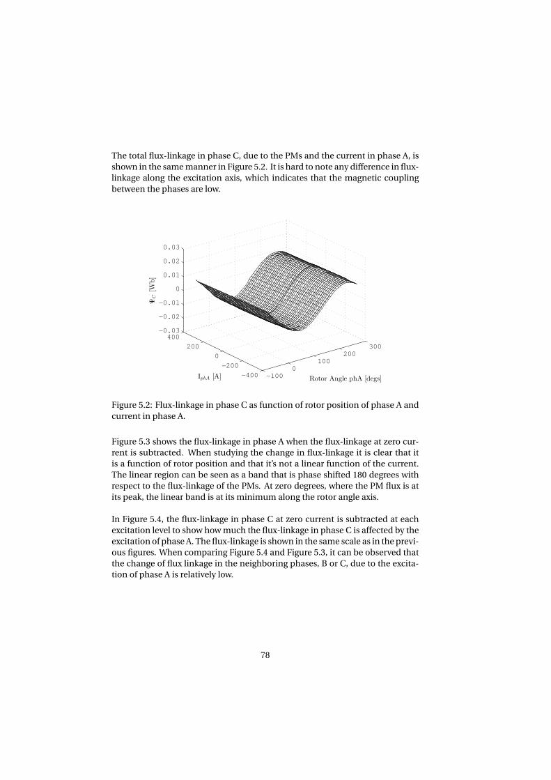
The total flux-linkage in phase C, due to the PMs and the current in phase A, is

shown in the same manner in Figure 5.2. It is hard to note any difference in flux-

linkage along the excitation axis, which indicates that the magnetic coupling

between the phases are low.

−1000

100200

300

−400

−200

0

200

400−0.03

−0.02

−0.01

0

0.01

0.02

0.03

Rotor Angle phA [degs]IphA [A]

ΨC[W

b]

Figure 5.2: Flux-linkage in phase C as function of rotor position of phase A and

current in phase A.

Figure 5.3 shows the flux-linkage in phase A when the flux-linkage at zero cur-

rent is subtracted. When studying the change in flux-linkage it is clear that it

is a function of rotor position and that it’s not a linear function of the current.

The linear region can be seen as a band that is phase shifted 180 degrees with

respect to the flux-linkage of the PMs. At zero degrees, where the PM flux is at

its peak, the linear band is at its minimum along the rotor angle axis.

In Figure 5.4, the flux-linkage in phase C at zero current is subtracted at each

excitation level to show how much the flux-linkage in phase C is affected by the

excitation of phase A. The flux-linkage is shown in the same scale as in the previ-

ous figures. When comparing Figure 5.4 and Figure 5.3, it can be observed that

the change of flux linkage in the neighboring phases, B or C, due to the excita-

tion of phase A is relatively low.

78

−1000

100200

300

−400

−200

0

200

400−0.03

−0.02

−0.01

0

0.01

0.02

0.03

Rotor Angle phA [degs]IphA [A]

∆Ψ

A[W

b]

Figure 5.3: The change of flux-linkage in phase A due to the current in phase A.

−1000

100200

300

−400

−200

0

200

400−0.03

−0.02

−0.01

0

0.01

0.02

0.03

Rotor Angle phA [degs]IphA [A]

∆Ψ

C[W

b]

Figure 5.4: The change of flux-linkage in phase C due to the current in phase A.

79

Figure 5.5 shows the ratio between the change of flux-linkage in phase C and the

change of flux-linkage in phase A, |∆ΨC /∆ΨA | in percent, due to the current in

phase A. If the the change in flux-linkage in phase A is assumed to be the total

induced flux, between 2.8% and 8.6% of the total induced flux in phase A links

the neighboring phases when they are unexcited. The average over the whole

map, excluding the points of zero excitation, is 4.6%.3

.5

3.5

3.5

3.5

3.5

3.54.

5

4.5

4.5

4.5

4.5

4.5

4.5

4.5

5.5

5.55.5

5.5

5.5

5.5

6.5

6.5

7.5

7.5

Rotor Angle phA [degs]

I phA[A

]

−50 0 50 100 150 200 250

−300

−200

−100

0

100

200

300

Figure 5.5: The ratio between the change in flux-linkage in phase C and the

change in flux-linkage in phase A, |∆ΨC /∆ΨA | in percent.

In Figure 5.6, the torque produced by a single phase as a function of its rotor

position and current is shown. Excluding the highest current levels, the peak

torque occur at exactly 90 electrical degrees, thus when the current is in the q-

direction.

80

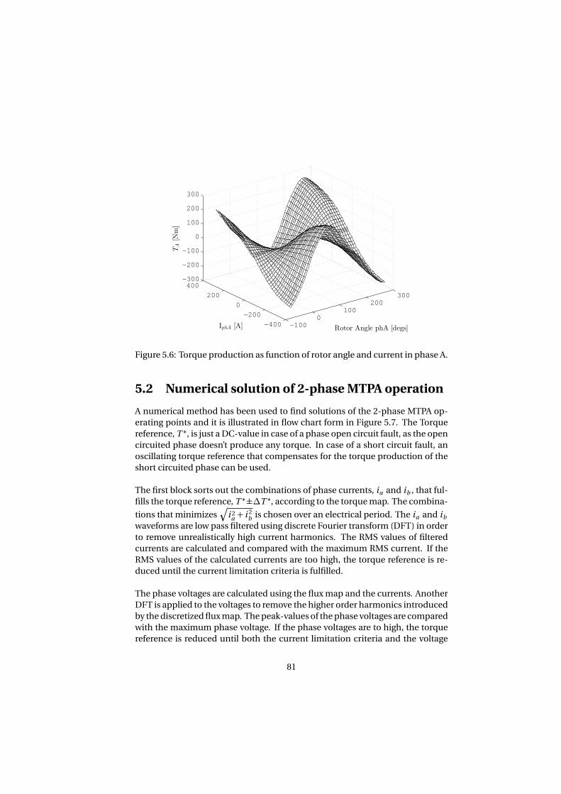
−1000

100200

300

−400

−200

0

200

400−300

−200

−100

0

100

200

300

Rotor Angle phA [degs]IphA [A]

TA[Nm]

Figure 5.6: Torque production as function of rotor angle and current in phase A.

5.2 Numerical solution of 2-phase MTPA operation

A numerical method has been used to find solutions of the 2-phase MTPA op-

erating points and it is illustrated in flow chart form in Figure 5.7. The Torque

reference, T ∗, is just a DC-value in case of a phase open circuit fault, as the open

circuited phase doesn’t produce any torque. In case of a short circuit fault, an

oscillating torque reference that compensates for the torque production of the

short circuited phase can be used.

The first block sorts out the combinations of phase currents, ia and ib , that ful-

fills the torque reference, T ∗±∆T ∗, according to the torque map. The combina-

tions that minimizesq

i 2a+ i 2

b is chosen over an electrical period. The ia and ib

waveforms are low pass filtered using discrete Fourier transform (DFT) in order

to remove unrealistically high current harmonics. The RMS values of filtered

currents are calculated and compared with the maximum RMS current. If the

RMS values of the calculated currents are too high, the torque reference is re-

duced until the current limitation criteria is fulfilled.

The phase voltages are calculated using the flux map and the currents. Another

DFT is applied to the voltages to remove the higher order harmonics introduced

by the discretized flux map. The peak-values of the phase voltages are compared

with the maximum phase voltage. If the phase voltages are to high, the torque

reference is reduced until both the current limitation criteria and the voltage

81

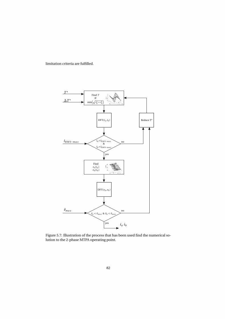
limitation criteria are fulfilled.

ia<iR M S−ma x

&ib<iR M S−ma x

iR M S−ma x

DFT(ia ,ib )

Find T@

minq

i 2a + i 2

b

T ∗

∆T ∗

DFT(va ,vb )

Reduce T*

vma xva < vma x & vb < vma x

Findva (ia )

vb (ib )

ia ib

no

yes

no

yes

Figure 5.7: Illustration of the process that has been used find the numerical so-

lution to the 2-phase MTPA operating point.

82

Chapter 6

Further analysis of one

fault-tolerant fractional slot

machine design

This chapter deals with the further analysis of one of the fault-tolerant PMSM

machine designs that are presented earlier in this thesis. When the machine

designs were evaluated in Chapter 4, machine B turned out to be a promising

design and it has thus been considered in the analysis of unbalanced operation

and the MMF harmonic content on the rotor side during balanced operation.

Some converter limitations related to some converter topologies were presented

briefly in Section 2.5, but the constraints related to the converter topologies are

not yet considered. Instead, the analysis of unbalanced operation has been

made from a machine perspective, where the same phase RMS current (250

AR M S ) and the same phase peak voltage (318 V) that are available during bal-

anced operation are just assumed to be available also during unbalanced con-

ditions as well. The analysis has been based on two different methods; in the

first method, the currents are arranged to maintain constant direct and quadra-

ture components in the dq0 reference frame, as presented in Section 2.4.2. The

first method takes only the fundamental frequency components into account

and does not include the different saturation levels of the phases during un-

balanced operation. Using the second method, that is based on the numerical

solution of operating points presented in Section 5.2, both the difference in sat-

uration level of the phases and several harmonic components are included.

83

6.1 Unbalanced operation using resonant controller

In this section, the ordinary PI controller together with the resonant controller

presented in Section 2.4.2 are used to find steady-state operating points when a

single phase open circuit fault or a single phase short circuit fault occurs. The

operating point that was found for the single phase open circuit fault is simu-

lated and analyzed also using transient FEA and using the per phase flux ma-

chine model described in Chapter 5.

6.1.1 Phase open circuit

The simulation that is to be analyzed is divided into three time periods, sep-

arated by the vertical dashed lines in the figures. The first part corresponds

to normal operation at 1300 rpm and the current references are put to; i ∗q=

150p

2/3 A and i ∗q= 0 A, controlled by only the PI controller. This operating

point has been chosen to illustrate an example where both the phase currents

and phase voltages are kept within the given boundaries. In the second part

phase C is opened close to its current peak and the current is controlled down

to zero as a first order system of 1 MHz bandwidth, mimicking an interruption

due to a open circuit fault. During the second part, the resonant controller is still

turned off and the PI controller alone, tries to reach the same current references

as in the first time period. In the third and last part, the resonant controller is

turned on while the current reference, i ∗q

, is reduced by a factor 1/p

3 to end up

with phase currents of the same magnitude as during the normal operation in

the first time period.

As the intention is to show the three steady-states in the same figures, the con-

trollers are tuned accordingly to achieve that. Therefore, the dynamic behavior

during the two transitions between the three time periods are not representa-

tive. As an example, a0 and a2 of the resonant controller, see Figure 2.2, are put

to zero according to [9]while a1 is put to a value high enough to quickly remove

the oscillations in id and iq .

The dq0 transformation of the phase currents are shown in Figure 6.1. During

normal operation, they are following their references as expected and the zero

sequence component is zero as it is a balanced three phase operating point.

When the fault occurs and phase C is opened, it can be seen that the PI controller

alone cannot control the currents according to the references and there are os-

cillations in all the dq0 components. In the third time period, when the resonant

controller is activated, the oscillations are removed from id and iq while only i0

is left oscillating.

84

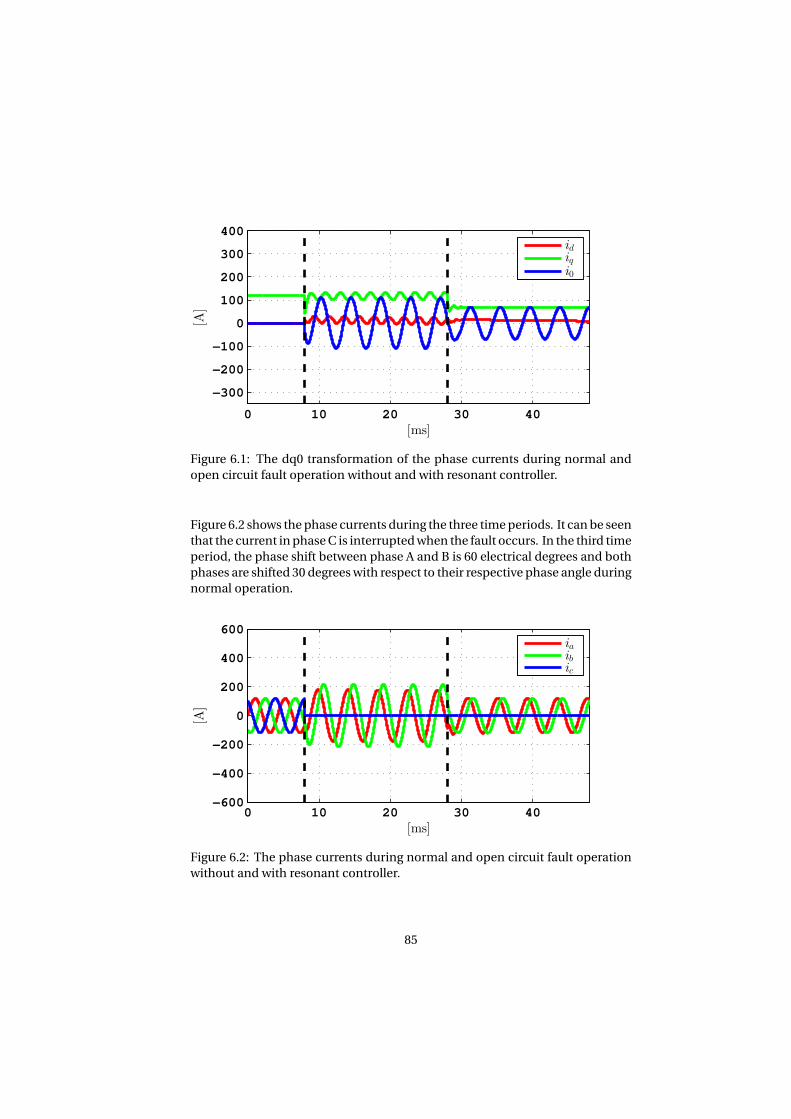
0 10 20 30 40

−300

−200

−100

0

100

200

300

400

[ms]

[A]

idiqi0

Figure 6.1: The dq0 transformation of the phase currents during normal and

open circuit fault operation without and with resonant controller.

Figure 6.2 shows the phase currents during the three time periods. It can be seen

that the current in phase C is interrupted when the fault occurs. In the third time

period, the phase shift between phase A and B is 60 electrical degrees and both

phases are shifted 30 degrees with respect to their respective phase angle during

normal operation.

0 10 20 30 40−600

−400

−200

0

200

400

600

[A]

[ms]

iaibic

Figure 6.2: The phase currents during normal and open circuit fault operation

without and with resonant controller.

85

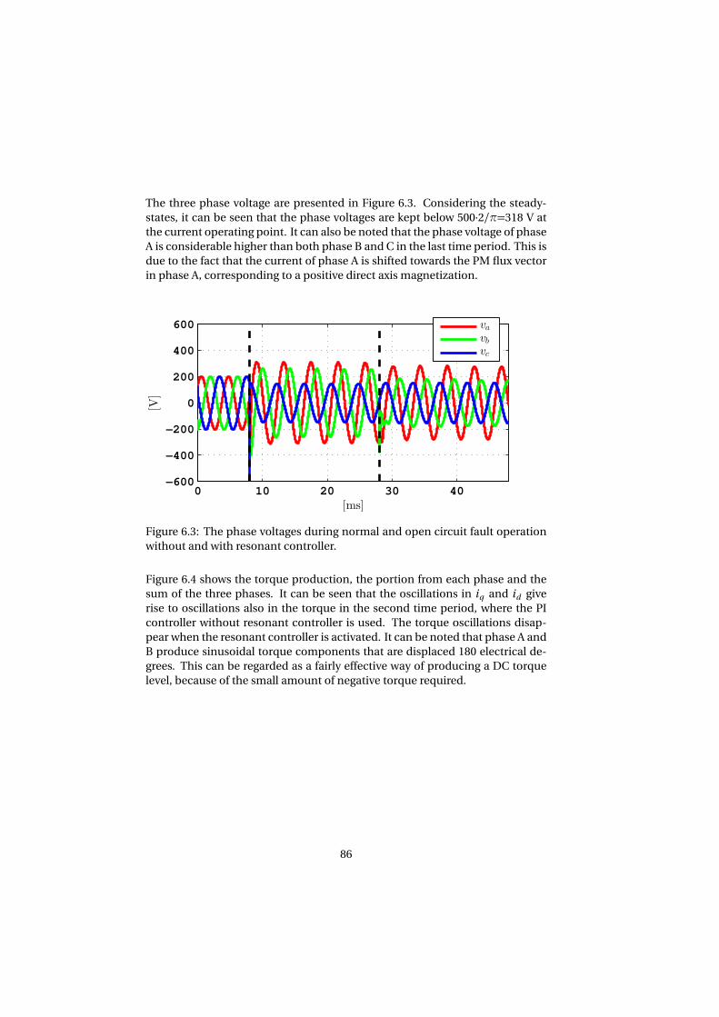
The three phase voltage are presented in Figure 6.3. Considering the steady-

states, it can be seen that the phase voltages are kept below 500·2/π=318 V at

the current operating point. It can also be noted that the phase voltage of phase

A is considerable higher than both phase B and C in the last time period. This is

due to the fact that the current of phase A is shifted towards the PM flux vector

in phase A, corresponding to a positive direct axis magnetization.

0 10 20 30 40−600

−400

−200

0

200

400

600

[V]

[ms]

vavbvc

Figure 6.3: The phase voltages during normal and open circuit fault operation

without and with resonant controller.

Figure 6.4 shows the torque production, the portion from each phase and the

sum of the three phases. It can be seen that the oscillations in iq and id give

rise to oscillations also in the torque in the second time period, where the PI

controller without resonant controller is used. The torque oscillations disap-

pear when the resonant controller is activated. It can be noted that phase A and

B produce sinusoidal torque components that are displaced 180 electrical de-

grees. This can be regarded as a fairly effective way of producing a DC torque

level, because of the small amount of negative torque required.

86

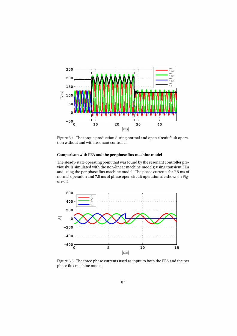
0 10 20 30 40−50

0

50

100

150

200

250

[Nm]

[ms]

Tea

Teb

Tec

Te

Figure 6.4: The torque production during normal and open circuit fault opera-

tion without and with resonant controller.

Comparison with FEA and the per phase flux machine model

The steady-state operating point that was found by the resonant controller pre-

viously, is simulated with the non-linear machine models; using transient FEA

and using the per phase flux machine model. The phase currents for 7.5 ms of

normal operation and 7.5 ms of phase open circuit operation are shown in Fig-

ure 6.5.

0 5 10 15−600

−400

−200

0

200

400

600

[A]

[ms]

iaibic

Figure 6.5: The three phase currents used as input to both the FEA and the per

phase flux machine model.

87

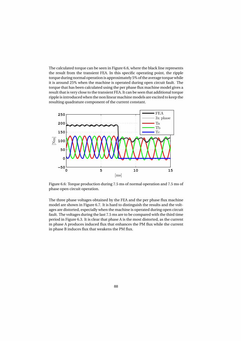
The calculated torque can be seen in Figure 6.6, where the black line represents

the result from the transient FEA. In this specific operating point, the ripple

torque during normal operation is approximately 5% of the average torque while

it is around 25% when the machine is operated during open circuit fault. The

torque that has been calculated using the per phase flux machine model gives a

result that is very close to the transient FEA. It can be seen that additional torque

ripple is introduced when the non linear machine models are excited to keep the

resulting quadrature component of the current constant.

0 5 10 15−50

0

50

100

150

200

250

[Nm]

[ms]

FEA3x phase

TaTbTc

Figure 6.6: Torque production during 7.5 ms of normal operation and 7.5 ms of

phase open circuit operation.

The three phase voltages obtained by the FEA and the per phase flux machine

model are shown in Figure 6.7. It is hard to distinguish the results and the volt-

ages are distorted, especially when the machine is operated during open circuit

fault. The voltages during the last 7.5 ms are to be compared with the third time

period in Figure 6.3. It is clear that phase A is the most distorted, as the current

in phase A produces induced flux that enhances the PM flux while the current

in phase B induces flux that weakens the PM flux.

88

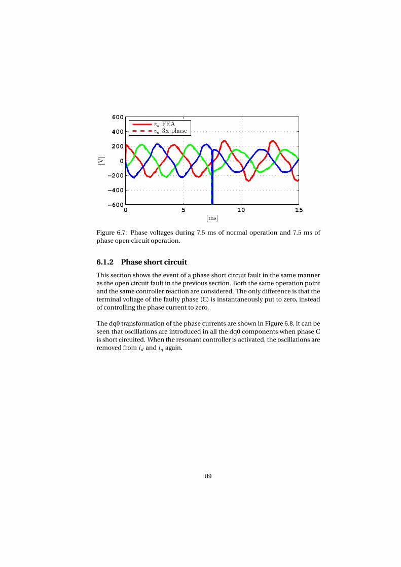
0 5 10 15−600

−400

−200

0

200

400

600

[V]

[ms]

va FEAva 3x phase

Figure 6.7: Phase voltages during 7.5 ms of normal operation and 7.5 ms of

phase open circuit operation.

6.1.2 Phase short circuit

This section shows the event of a phase short circuit fault in the same manner

as the open circuit fault in the previous section. Both the same operation point

and the same controller reaction are considered. The only difference is that the

terminal voltage of the faulty phase (C) is instantaneously put to zero, instead

of controlling the phase current to zero.

The dq0 transformation of the phase currents are shown in Figure 6.8, it can be

seen that oscillations are introduced in all the dq0 components when phase C

is short circuited. When the resonant controller is activated, the oscillations are

removed from id and iq again.

89

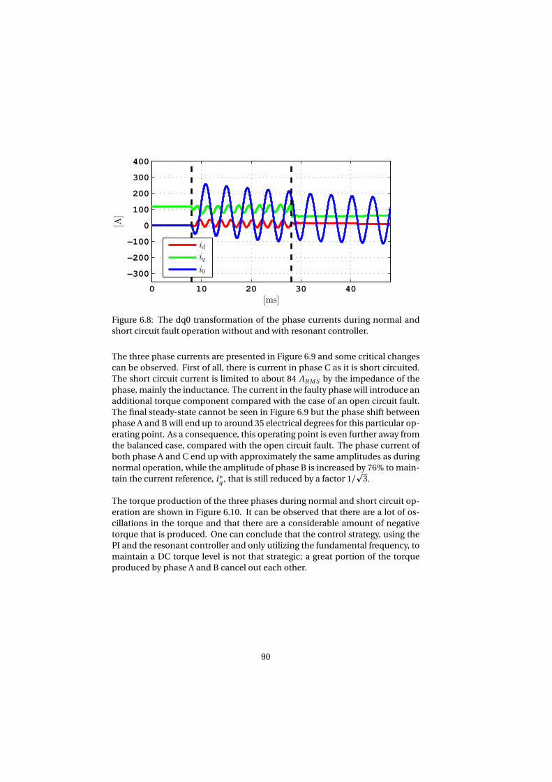
0 10 20 30 40

−300

−200

−100

0

100

200

300

400

[ms]

[A]

idiqi0

Figure 6.8: The dq0 transformation of the phase currents during normal and

short circuit fault operation without and with resonant controller.

The three phase currents are presented in Figure 6.9 and some critical changes

can be observed. First of all, there is current in phase C as it is short circuited.

The short circuit current is limited to about 84 AR M S by the impedance of the

phase, mainly the inductance. The current in the faulty phase will introduce an

additional torque component compared with the case of an open circuit fault.

The final steady-state cannot be seen in Figure 6.9 but the phase shift between

phase A and B will end up to around 35 electrical degrees for this particular op-

erating point. As a consequence, this operating point is even further away from

the balanced case, compared with the open circuit fault. The phase current of

both phase A and C end up with approximately the same amplitudes as during

normal operation, while the amplitude of phase B is increased by 76% to main-

tain the current reference, i ∗q

, that is still reduced by a factor 1/p

3.

The torque production of the three phases during normal and short circuit op-

eration are shown in Figure 6.10. It can be observed that there are a lot of os-

cillations in the torque and that there are a considerable amount of negative

torque that is produced. One can conclude that the control strategy, using the

PI and the resonant controller and only utilizing the fundamental frequency, to

maintain a DC torque level is not that strategic; a great portion of the torque

produced by phase A and B cancel out each other.

90

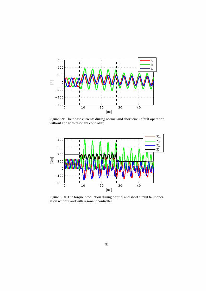
0 10 20 30 40−600

−400

−200

0

200

400

600

[A]

[ms]

iaibic

Figure 6.9: The phase currents during normal and short circuit fault operation

without and with resonant controller.

0 10 20 30 40−200

−100

0

100

200

300

400

[Nm]

[ms]

Tea

Teb

Tec

Te

Figure 6.10: The torque production during normal and short circuit fault oper-

ation without and with resonant controller.

91

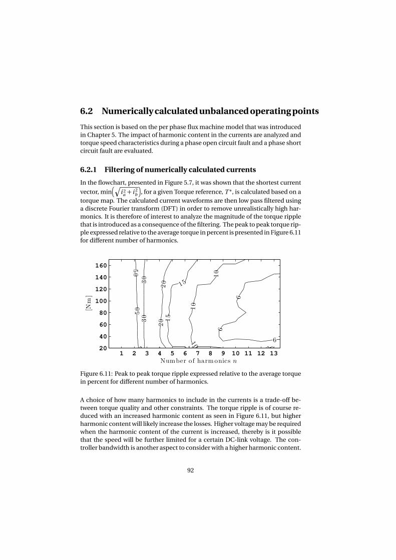
6.2 Numerically calculated unbalanced operating points

This section is based on the per phase flux machine model that was introduced

in Chapter 5. The impact of harmonic content in the currents are analyzed and

torque speed characteristics during a phase open circuit fault and a phase short

circuit fault are evaluated.

6.2.1 Filtering of numerically calculated currents

In the flowchart, presented in Figure 5.7, it was shown that the shortest current

vector, minq

i 2a+ i 2

b

, for a given Torque reference, T ∗, is calculated based on a

torque map. The calculated current waveforms are then low pass filtered using

a discrete Fourier transform (DFT) in order to remove unrealistically high har-

monics. It is therefore of interest to analyze the magnitude of the torque ripple

that is introduced as a consequence of the filtering. The peak to peak torque rip-

ple expressed relative to the average torque in percent is presented in Figure 6.11

for different number of harmonics.6

6

6

10

10

10

10

15

15

15 15

20

20

20 20

30

30

30

50

50

5

[Nm]

Number of harmonics n1 2 3 4 5 6 7 8 9 10 11 12 13

20

40

60

80

100

120

140

160

Figure 6.11: Peak to peak torque ripple expressed relative to the average torque

in percent for different number of harmonics.

A choice of how many harmonics to include in the currents is a trade-off be-

tween torque quality and other constraints. The torque ripple is of course re-

duced with an increased harmonic content as seen in Figure 6.11, but higher

harmonic content will likely increase the losses. Higher voltage may be required

when the harmonic content of the current is increased, thereby is it possible

that the speed will be further limited for a certain DC-link voltage. The con-

troller bandwidth is another aspect to consider with a higher harmonic content.

92

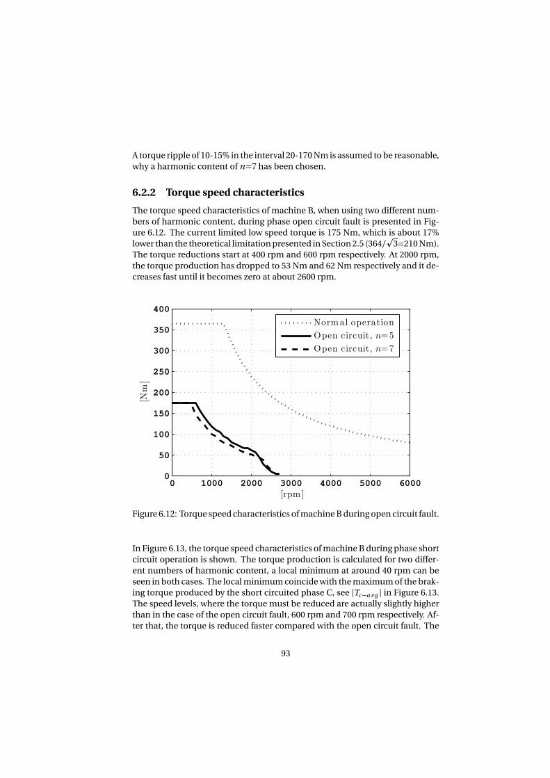
A torque ripple of 10-15% in the interval 20-170 Nm is assumed to be reasonable,

why a harmonic content of n=7 has been chosen.

6.2.2 Torque speed characteristics

The torque speed characteristics of machine B, when using two different num-

bers of harmonic content, during phase open circuit fault is presented in Fig-

ure 6.12. The current limited low speed torque is 175 Nm, which is about 17%

lower than the theoretical limitation presented in Section 2.5 (364/p

3=210 Nm).

The torque reductions start at 400 rpm and 600 rpm respectively. At 2000 rpm,

the torque production has dropped to 53 Nm and 62 Nm respectively and it de-

creases fast until it becomes zero at about 2600 rpm.

0 1000 2000 3000 4000 5000 60000

50

100

150

200

250

300

350

400

[Nm]

[rpm ]

Normal operation

Open circuit, n=5

Open circuit, n=7

Figure 6.12: Torque speed characteristics of machine B during open circuit fault.

In Figure 6.13, the torque speed characteristics of machine B during phase short

circuit operation is shown. The torque production is calculated for two differ-

ent numbers of harmonic content, a local minimum at around 40 rpm can be

seen in both cases. The local minimum coincide with the maximum of the brak-

ing torque produced by the short circuited phase C, see |Tc−a v g | in Figure 6.13.

The speed levels, where the torque must be reduced are actually slightly higher

than in the case of the open circuit fault, 600 rpm and 700 rpm respectively. Af-

ter that, the torque is reduced faster compared with the open circuit fault. The

93

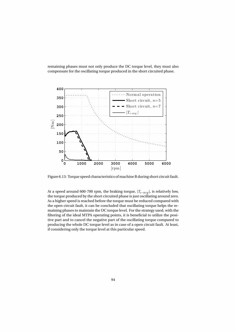
remaining phases must not only produce the DC torque level, they must also

compensate for the oscillating torque produced in the short circuited phase.

0 1000 2000 3000 4000 5000 60000

50

100

150

200

250

300

350

400

[Nm]

[rpm ]

Normal operation

Short circuit, n=5

Short circuit, n=7

|Tc−avg |

Figure 6.13: Torque speed characteristics of machine B during short circuit fault.

At a speed around 600-700 rpm, the braking torque, |Tc−a v g |, is relatively low,

the torque produced by the short circuited phase is just oscillating around zero.

As a higher speed is reached before the torque must be reduced compared with

the open circuit fault, it can be concluded that oscillating torque helps the re-

maining phases to maintain the DC torque level. For the strategy used, with the

filtering of the ideal MTPA operating points, it is beneficial to utilize the posi-

tive part and to cancel the negative part of the oscillating torque compared to

producing the whole DC torque level as in case of a open circuit fault. At least,

if considering only the torque level at this particular speed.

94

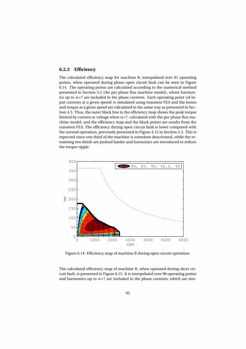
6.2.3 Efficiency

The calculated efficiency map for machine B, interpolated over 81 operating

points, when operated during phase open circuit fault can be seen in Figure

6.14. The operating points are calculated according to the numerical method

presented in Section 5.2 (the per phase flux machine model), where harmon-

ics up to n=7 are included in the phase currents. Each operating point (of in-

put currents at a given speed) is simulated using transient FEA and the losses

and torque at a given speed are calculated in the same way as presented in Sec-

tion 4.3. Thus, the outer black line in the efficiency map shows the peak torque

limited by current or voltage when n=7, calculated with the per phase flux ma-

chine model, and the efficiency map and the black points are results from the

transient FEA. The efficiency during open circuit fault is lower compared with

the normal operation, prevously presented in Figure 4.12 in Section 4.3. This is

expected since one third of the machine is somehow deactivated, while the re-

maining two thirds are pushed harder and harmonics are introduced to reduce

the torque ripple.

80 80

8080

85

85

8585

90

90

9090

92.5

92.592.5

95

95

rpm

Nm

0 1000 2000 3000 4000 5000 60000

50

100

150

200

250

300

350

40080, 85, 90, 92.5, 95

Figure 6.14: Efficiency map of machine B during open circuit operation.

The calculated efficiency map of machine B, when operated during short cir-

cuit fault, is presented in Figure 6.15. It is interpolated over 90 operating points

and harmonics up to n=7 are included in the phase currents, which are sim-

95

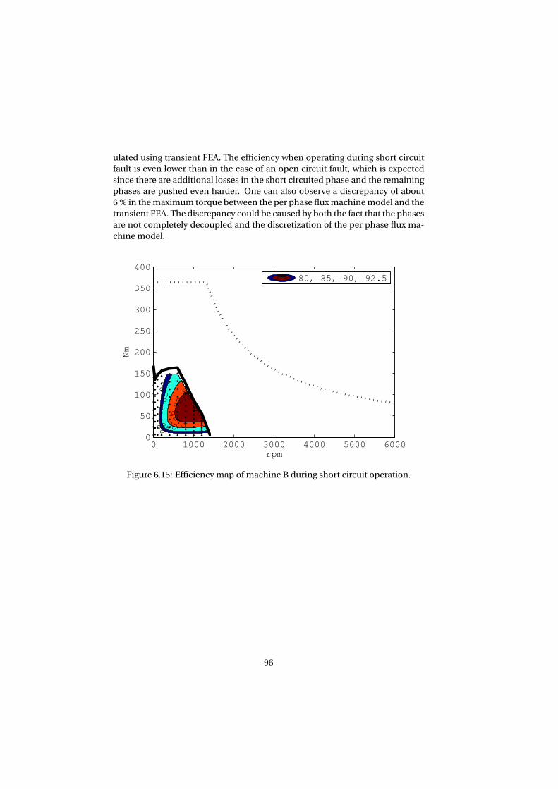
ulated using transient FEA. The efficiency when operating during short circuit

fault is even lower than in the case of an open circuit fault, which is expected

since there are additional losses in the short circuited phase and the remaining

phases are pushed even harder. One can also observe a discrepancy of about

6 % in the maximum torque between the per phase flux machine model and the

transient FEA. The discrepancy could be caused by both the fact that the phases

are not completely decoupled and the discretization of the per phase flux ma-

chine model.

80

80

80

85 85

85

90

90

92.5

92.5

rpm

Nm

0 1000 2000 3000 4000 5000 60000

50

100

150

200

250

300

350

40080, 85, 90, 92.5

Figure 6.15: Efficiency map of machine B during short circuit operation.

96

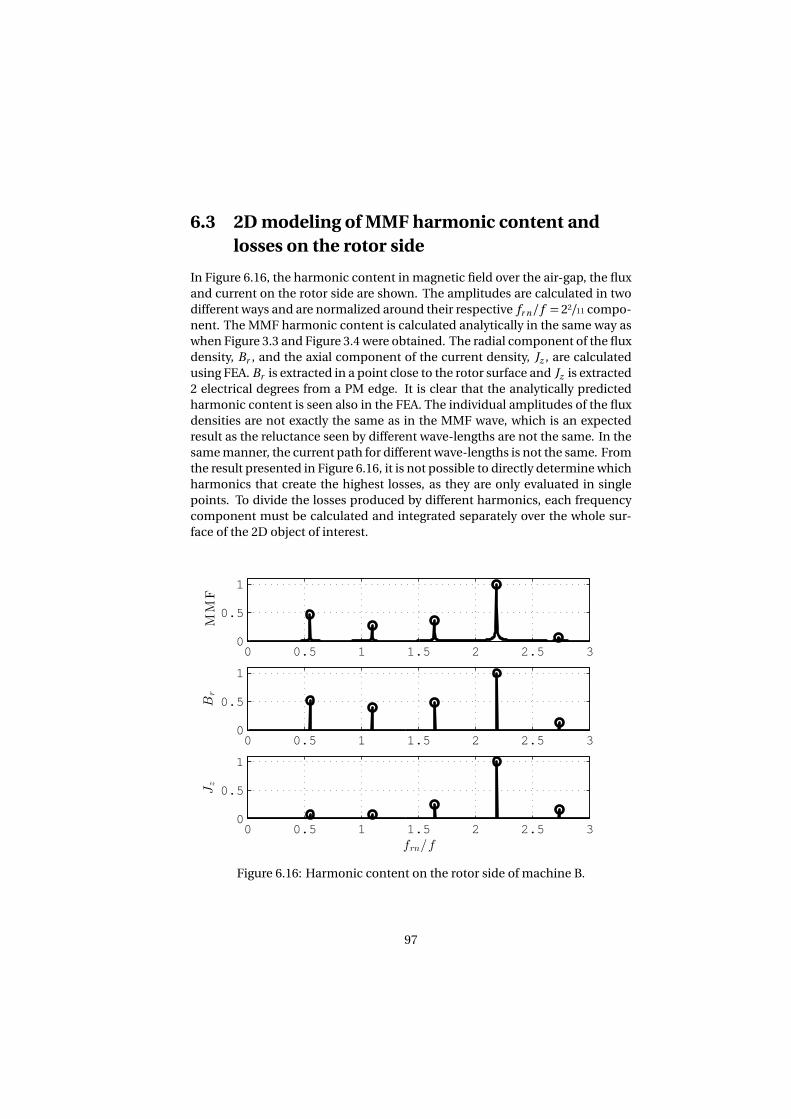
6.3 2D modeling of MMF harmonic content and

losses on the rotor side

In Figure 6.16, the harmonic content in magnetic field over the air-gap, the flux

and current on the rotor side are shown. The amplitudes are calculated in two

different ways and are normalized around their respective fr n/ f = 22/11 compo-

nent. The MMF harmonic content is calculated analytically in the same way as

when Figure 3.3 and Figure 3.4 were obtained. The radial component of the flux

density, Br , and the axial component of the current density, Jz , are calculated

using FEA. Br is extracted in a point close to the rotor surface and Jz is extracted

2 electrical degrees from a PM edge. It is clear that the analytically predicted

harmonic content is seen also in the FEA. The individual amplitudes of the flux

densities are not exactly the same as in the MMF wave, which is an expected

result as the reluctance seen by different wave-lengths are not the same. In the

same manner, the current path for different wave-lengths is not the same. From

the result presented in Figure 6.16, it is not possible to directly determine which

harmonics that create the highest losses, as they are only evaluated in single

points. To divide the losses produced by different harmonics, each frequency

component must be calculated and integrated separately over the whole sur-

face of the 2D object of interest.

0 0.5 1 1.5 2 2.5 30

0.5

1

Jz

frn/f

0 0.5 1 1.5 2 2.5 30

0.5

1

MM

F

0 0.5 1 1.5 2 2.5 30

0.5

1

Br

Figure 6.16: Harmonic content on the rotor side of machine B.

97

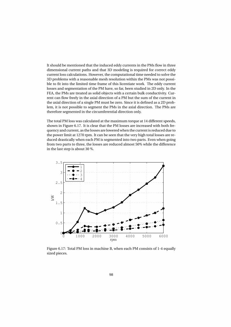
It should be mentioned that the induced eddy currents in the PMs flow in three

dimensional current paths and that 3D modeling is required for correct eddy

current loss calculations. However, the computational time needed to solve the

3D problems with a reasonable mesh resolution within the PMs was not possi-

ble to fit into the limited time frame of this licentiate work. The eddy current

losses and segmentation of the PM have, so far, been studied in 2D only. In the

FEA, the PMs are treated as solid objects with a certain bulk conductivity. Cur-

rent can flow freely in the axial direction of a PM but the sum of the current in

the axial direction of a single PM must be zero. Since it is defined as a 2D prob-

lem, it is not possible to segment the PMs in the axial direction. The PMs are

therefore segmented in the circumferential direction only.

The total PM loss was calculated at the maximum torque at 14 different speeds,

shown in Figure 6.17. It is clear that the PM losses are increased with both fre-

quency and current, as the losses are lowered when the current is reduced due to

the power limit at 1270 rpm. It can be seen that the very high total losses are re-

duced drastically when each PM is segmented into two parts. Even when going

from two parts to three, the losses are reduced almost 50% while the difference

in the last step is about 30 %.

0 1000 2000 3000 4000 5000 60000

0.5

1

1.5

2

2.5

3

3.5

rpm

kW

1234

Figure 6.17: Total PM loss in machine B, when each PM consists of 1-4 equally

sized pieces.

98

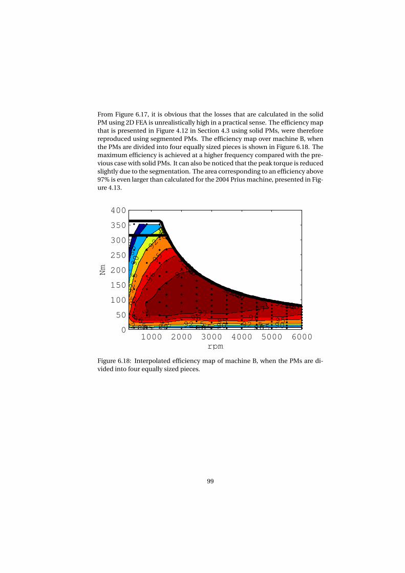
From Figure 6.17, it is obvious that the losses that are calculated in the solid

PM using 2D FEA is unrealistically high in a practical sense. The efficiency map

that is presented in Figure 4.12 in Section 4.3 using solid PMs, were therefore

reproduced using segmented PMs. The efficiency map over machine B, when

the PMs are divided into four equally sized pieces is shown in Figure 6.18. The

maximum efficiency is achieved at a higher frequency compared with the pre-

vious case with solid PMs. It can also be noticed that the peak torque is reduced

slightly due to the segmentation. The area corresponding to an efficiency above

97% is even larger than calculated for the 2004 Prius machine, presented in Fig-

ure 4.13.

808080

80

80

80

80

8080

858585

85

85

85

85

8585

909090

90

90

90

90

9090

92.592.592.5

92.5

92.5

92.5

92.592.5

959595

95

95

95

9595

969696

96

96

9696

97

97

9797

97

rpm

Nm

1000 2000 3000 4000 5000 60000

50

100

150

200

250

300

350

400

Figure 6.18: Interpolated efficiency map of machine B, when the PMs are di-

vided into four equally sized pieces.

99

100

Chapter 7

Conclusions and future work

7.1 Conclusions

In this thesis, a fault-tolerant fractional slot machine with a similar size and per-

formance as the Toyota Prius 2004 reference machine is designed. The faults in-

vestigated are phase open circuit and phase short circuit, and it is shown that the

thesis machine design can be operated during both circumstances. The elec-

tromagnetic design of the machines have been compared with the use of 2D fi-

nite element analysis; the calculated overall efficiency of the final thesis design

turned out to be slightly higher than that of the 2004 Prius design, in case of

segmented permanent magnets. The estimated material cost to produce a ma-

chine is included already in the design process, where four design variables are

varied. In that way, the most promising designs considering both performance

and cost were sorted out. The estimated material cost of the finally selected

machine design is about 8% higher and the peak torque slightly lower (364 Nm)

than the 2004 Prius design (374 Nm).

It has been shown that the torque ripple of a PMSM may increase when operated

under unbalanced conditions and the phase currents are controlled in the clas-

sical vector control manner to maintain a constant torque producing quadra-

ture axis current in the dq0 reference frame. A semi-analytical machine mod-

eling approach is used to model the individual saturation levels of the phases

successfully. Harmonics can be included in the phase currents to increase the

torque quality but the area of possible operating points is reduced substantially.

The maximum torque is reduced by approximately 50% and can be maintained

up to about 600 rpm in case of an open circuit fault, compared to about 1300 rpm

at normal operation. In case of a short circuit fault, the maximum torque varies

within the whole speed operating range, due to the braking torque produced by

the short circuited phase. The starting torque, when the short circuit torque is

101

negligible, is of course reduced to approximately 50% also in case of a short cir-

cuit fault. Without a constant speed load profile, it is not possible to determine

the reduction of the maximum vehicle speed; but in rough numbers about 1/3

or slightly below 1/4 of the maximum speed of 6000 rpm during normal opera-

tion, in case of an open circuit fault or a short circuit fault respectively, is what

is achievable.

102

7.2 Future Work

Here follow some suggestions for future work, either parts that were consciously

not included in this work or as reflection over the thesis and its results.

• When the cost efficiency of the electric machine designs were evaluated,

only the torque production at low speed was included. It is possible to im-

prove the process by adding more properties in order to sort out the most

promising candidates in a more effective manner. For example, the field

weakening characteristics and the thermal restrictions of electric loading

could be evaluated at the same time. It is also possible to reformulate the

constraint instead of using a single break point of above 95% of the maxi-

mum torque output per cost.

• Investigate the effect of the DC-link current ripple in relation to both per-

formance and comfort when operating during fault.

• Model the eddy current loss in the permanent magnets and evaluate seg-

mentation using 3D finite element analysis, both during normal opera-

tion and operation during a fault.

• Further thermal analysis, using less simplified models.

• Complete electric drive system modeling including both machine and con-

verter models but also the control and fault detection.

• There are commercial fractional slot concentrated winding PMSM avail-

able on the market, some of them are potentially of suitable pole/slot con-

figurations for unbalanced operation during fault. That would be interest-

ing to investigate and test in the lab.

• Compare the results with other fault-tolerant solutions; it could be multi-

phase systems with a separate converter and machine or modular systems

where the winding terminals are attached directly to the power electron-

ics.

• Combine an electric drive system model with a vehicle model in order to

evaluate fault-tolerant vehicle performance more precisely.

• Analyze how the machine performance during fault is affected in case of

a PMSM with interior-mounted permanent magnets instead of surface-

mounted permanent magnets.

103

104

Bibliography

[1] D. Diallo, M. Benbouzid, and A. Makouf, “A fault-tolerant control archi-

tecture for induction motor drives in automotive applications,” Vehicular

Technology, IEEE Transactions on, vol. 53, no. 6, pp. 1847–1855, Nov 2004.

[2] A. Jack, B. Mecrow, and J. Haylock, “A comparative study of perma-

nent magnet and switched reluctance motors for high-performance fault-

tolerant applications,” Industry Applications, IEEE Transactions on, vol. 32,

no. 4, pp. 889–895, Jul 1996.

[3] N. Bianchi and S. Bolognani, “Fault -tolerant pm motors in automotive ap-

plications,” in Vehicle Power and Propulsion, 2005 IEEE Conference, Sept

2005, pp. 747–755.

[4] M. Abolhassani and H. Toliyat, “Fault tolerant permanent magnet motor

drives for electric vehicles,” in Electric Machines and Drives Conference,

2009. IEMDC ’09. IEEE International, May 2009, pp. 1146–1152.

[5] A. EL-Refaie, “Fractional-slot concentrated-windings synchronous perma-

nent magnet machines: Opportunities and challenges,” Industrial Elec-

tronics, IEEE Transactions on, vol. 57, no. 1, pp. 107–121, Jan 2010.

[6] E. Fornasiero, Advanced Design of Direct Drive PM Machines. Ph.D. thesis,

Department of Electrical Engineering, University of Padova, Padova,Italy,

2010.

[7] G. Dajaku and D. Gerling, “Low costs and high-efficiency electric ma-

chines,” in Electric Drives Production Conference (EDPC), 2012 2nd Inter-

national, Oct 2012, pp. 1–7.

[8] M. Barcaro, N. Bianchi, E. Fornasiero, and F. Magnussen, “Experimental

comparison between two fault-tolerant fractional-slot multiphase pm mo-

tor drives,” in Industrial Electronics (ISIE), 2010 IEEE International Sympo-

sium on, July 2010, pp. 2160–2165.

105

[9] Y. Crevits, X. Kestelyn, and E. Semail, “Investigation on vector control

of three-phase synchronous machines under supply fault condition,”

in Power Electronics, Electrical Drives, Automation and Motion, 2006.

SPEEDAM 2006. International Symposium on, May 2006, pp. 439–444.

[10] C. Gajanayake, B. Bhangu, S. Nadarajan, and G. Jayasinghe, “Fault tolerant

control method to improve the torque and speed response in pmsm drive

with winding faults,” in Power Electronics and Drive Systems (PEDS), 2011

IEEE Ninth International Conference on, Dec 2011, pp. 956–961.

[11] N. Bianchi, S. Bolognani, M. Zigliotto, and M. Zordan, “Innovative reme-

dial strategies for inverter faults in ipm synchronous motor drives,” Energy

Conversion, IEEE Transactions on, vol. 18, no. 2, pp. 306–314, June 2003.

[12] N. Bianchi, S. Bolognani, and M. Zigliotto, “Analysis of pm synchronous

motor drive failures during flux weakening operation,” in Power Electronics

Specialists Conference, 1996. PESC ’96 Record., 27th Annual IEEE, vol. 2, Jun

1996, pp. 1542–1548 vol.2.

[13] A. Krings and J. Soulard, “Overview and comparison of iron loss models

for electrical machines,” Journal of Electrical Engineering, vol. 10, no. 3,

pp. 162–169, 2010, updated and revised version of conference paper from

the 5th International Conference and Exhibition on Ecological Vehicles

and Renewable Energies (EVER 10), Monte-Carlo, MONACO, MAR 25-28,

2010QC 20120120.

[14] L. Svensson, M. Andersson, A. Reinap, and M. Alaküla, “Thermal proper-

ties on high fill factor electrical windings: Infiltrated vs non infiltrated,” In-

ternational Conference on Electrical Machines (ICEM14), Berlin, Germany,

Sep 2014.

[15] A. Jack, B. Mecrow, P. Dickinson, D. Stephenson, J. Burdess, J. N. Fawcett,

and T. Evans, “Permanent magnet machines with powdered iron cores and

pre-pressed windings,” in Industry Applications Conference, 1999. Thirty-

Fourth IAS Annual Meeting. Conference Record of the 1999 IEEE, vol. 1, 1999,

pp. 97–103 vol.1.

[16] R. Wrobel, P. Mellor, and D. Holliday, “Thermal modeling of a segmented

stator winding design,” Industry Applications, IEEE Transactions on, vol. 47,

no. 5, pp. 2023–2030, Sept 2011.

[17] H. J.R. and M. T.J.E, Design Of Brushless Permanent-Magnet Machines. Mo-

tor Design Books LLC, Florida, 2010.

[18] J. Gieras, M. Kamper, and R.-J. Wang, Axial Flux Permanent Magnet Brush-

less Machines 2nd Edition. Springer Science & Business Media B.V., 2008.

106

[19] C. Liwschitz-Garik, M. assisted by Clyde and E. Whipple, Electric Machin-

ery, Volume 2 A-C Machines. Van Nordstrand, New York, 1946.

[20] G. Dajaku, D. Gerling, and W. Xie, “Reduction of low space harmonics for

the fractional slot concentrated windings using a novel stator design,” Mag-

netics, IEEE Transactions on, vol. PP, no. 99, pp. 1–1, 2013.

[21] T. D. Strous, H. Polinder, and J. Ferreira, “Inductance calculations for pm

machines with concentrated windings,” in Electric Machines Drives Con-

ference (IEMDC), 2011 IEEE International, May 2011, pp. 447–452.

[22] R. Krishnan, Permanent Magnet Synchronous and Brushless DC Motor

Drives. Hoboken: CRC Press, 2009. [Online]. Available: www.summon.

com

[23] L. Chong, R. Dutta, N. Dai, M. Rahman, and H. Lovatt, “Comparison of con-

centrated and distributed windings in an ipm machine for field weakening

applications,” in Universities Power Engineering Conference (AUPEC), 2010

20th Australasian, Dec 2010, pp. 1–5.

[24] T. A. O. Burress, S. L. O. Campbell, C. O. Coomer, C. W. O. Ayers, A. A. O.

Wereszczak, J. P. O. Cunningham, L. D. O. Marlino, L. E. O. Seiber, and H.-

T. O. Lin, Evaluation of the 2010 Toyota Prius Hybrid Synergy Drive System,

Mar 2011. [Online]. Available: http://www.osti.gov/scitech/servlets/purl/

1007833

[25] ANSYS, “Study of a permanent magnet motor with maxwell 2d : Example

of the 2004 prius ipm motor,” unpublished. [Online]. Available: http:

//www.ansys.com

[26] R. Staunton, C. Ayers, J. U. T.-K. Chiasson, B. O. Burress, and L. Marlino,

Evaluation of 2004 Toyota Prius Hybrid Electric Drive System, May 2006.

[Online]. Available: http://www.osti.gov/scitech/servlets/purl/890029

[27] J. Hsu, Report on Toyota Prius Motor Thermal Management, Feb 2005.

[Online]. Available: http://www.osti.gov/scitech/servlets/purl/885987

[28] J. Li, D.-W. Choi, D.-H. Son, and Y.-H. Cho, “Effects of mmf harmonics on ro-

tor eddy-current losses for inner-rotor fractional slot axial flux permanent

magnet synchronous machines,” Magnetics, IEEE Transactions on, vol. 48,

no. 2, pp. 839–842, Feb 2012.

[29] (2014, Okt) Arnold Magnetic Technologies. Accessed 2014-10-13.

[Online]. Available: http://www.arnoldmagnetics.com/Neodymium_

Literature.aspx

[30] (2014, Aug) Metalprices.com. Accessed 2014-08-05. [Online]. Available:

http://www.metalprices.com/dailysnapshots/Index

107

[31] (2014, Aug) Metal-pages.com. Accessed 2014-08-05. [Online]. Available:

http://www.metal-pages.com/

[32] (2011, Dec) Critical materials strategy. U.S. Department of energy. Accessed

2014-08-05. [Online]. Available: http://www.arnoldmagnetics.com/Rare\

_Earth\_Information.aspx

[33] (2012, jan) The important role of dysprosium in modern permanent

magnets. Arnold Magnetic Technologies. Accessed 2014-08-05. [Online].

Available: http://www.arnoldmagnetics.com/Rare\_Earth\_Information.

aspx

[34] J. Hsu, Report on Toyota/Prius Motor Design and Manufacturing Assess-

ment, Jul 2004. [Online]. Available: http://www.osti.gov/scitech/servlets/

purl/885676

[35] K. Kiyota, H. Sugimoto, and A. Chiba, “Comparing electric motors: An anal-

ysis using four standard driving schedules,” Industry Applications Maga-

zine, IEEE, vol. 20, no. 4, pp. 12–20, July 2014.

108