1 Tangent Space Vectors and Tensors

1.1 Representations

At each point P of a manifoldM , there is a tangent space TP of vectors. Choos-ing a set of basis vectors e� 2 TP provides a representation of each vector u 2 TPin terms of components u�.

u = u�e�= u0e0 + u

1e1 + u2e2 + :::

= [u] [e]

where the last expression treats the basis vectors as a column matrix [e] andthe vector components as a row matrix [u].There is also a cotangent space T̂P of one-forms at each point. The basis

one-forms which are dual to the basis vectors e� are just the component-takingoperators:

!� (u) = !� � u = u � !� = u�

or, in terms of a row matrix [!] of basis forms,

u � [!] = [u] :

When one of these operators acts on a basis vector, it produces one or zeroaccording to:

!� (e�) = ���

or, in matrix notation,[e] � [!] = [1]

An arbitrary one-form ' can be represented by its components '� in the form:

' = '�!� = [!] [']

where the components are now arranged as a column matrix.Here are various ways to represent a form acting on a vector to give a number:

' (u) = u (') = ' � u = u � ' = u�'�= u0'0 + u

1'1 + u2'2 + u

3'3 + :::= ['] [u]

1.2 Holonomic Basis

Given a coordinate patch � a set of independent functions x� which can beused to label points in some part of M � a special set of basis one-forms canbe de�ned: !� = dx�

dx� (u) = u (x�)

Recall that each tangent vector u is really a directional derivative.

u =d

d�

����C

1

where C is a curve whose tangent vector at P is u. Rewrite the de�nition ofthe dx� in various ways:

dx� � u = u � dx� = dx� (u) =dx� (C (�))

d�

The basis vectors dual to the one-forms dx� are just our old friends thepartial derivatives:

@� =@

@x�

This type of basis is called a holonomic basis. For a vector u, here are variousexpressions in such a basis:

u = u�@�; u� = dx� � uu� = u (x�) = dx�

d� = _x�

u = _x�@� =dx�

d�

@

@x�

For a one-form ' here are various expressions in a holonomic basis:

' = '�dx� ; '� = ' � @�

df � @� =@f

@x�; df =

@f

@x�dx�

Some more expressions in a holonomic basis:

u � ' = (u�@�) ��'�dx

��= u�'�

u � df = u� (df)� =dx�

d�

@f

@x�

u � df = u (f) =df

d�

1.3 n-beins, Vierbeins, Tetrads, etc.

Holonomic bases are not always appropriate. For example, local observers al-ways want to use orthonormal basis vectors but it is not usually possible for aholonomic basis system to be orthonormal everywhere. However, if one has acurve C which is de�ned in terms of coordinates and wants its tangent vector,then the holonomic basis is needed. Thus, non-holonomic basis systems areusually related to holonomic ones like this:

ea = ba�@� ; !a = dx�b�

a

with the inverse relations:

@� = b�beb; dx� = !bbb

�

2

Here, I am using Latin indexes for the non-holonomic basis and Greek indexesfor the holonomic basis. Sometimes the two kinds of indexes are distinguishedin other ways:

e(�) = b(�)�@� ; !(�) = dx�b�

(�)

Underlines, primes, carets, and other doodads are used to mark one set ofindexes as distinct from the other. Notice that the index positions are absolutelycritical. If you are using Scienti�c Notebook or Scienti�c Workplace, you need toprevent superscripts and subscripts from lining up one over the other by insertinga zero space between them.In terms of matrices, the relation between holonomic and non-holonomic

representations would look like this:

[e] = [b] [@] ; [!] = [dx] [b]�1

[@] = [b]�1[e] ; [dx] = [!] [b]

Here are the non-holonomic components of the velocity of a particle whichis located at coordinates xi (t) at time t:

v = va@a = vaba(a)e(a) = v(a)e(a)

v(a) = vaba(a)

va =dxa

dt= _xa

v(a) = _xaba(a)

In a four-dimensional spacetime, a non-holonomic basis system is often calleda tetrad or a vierbein or a moving frame. The two types of indexes are notalways integrated into a single formalism connected by tetrad coe¢ cients ba(a).Sometimes we just perform a change of basis when it is convenient but use onlyone type of basis at a time.

1.4 Higher rank tensors

Vectors and one-forms are special cases of tensors. Higher rank tensors aremultilinear functions of vectors and one-forms. They can be built up fromtensor products de�ned like this:

u v (�; �) = u (�) v (�) ; � � (u; v) = � (u)� (v)

u � ' (�; u; v) = u (�)� (u)' (v)

The space of tensors that act on pairs of vectors can be built from the tensorproducts

e�� = e� e�and is designated TP TP . Other tensors are built up similarly. An example ofsuch a tensor would be

T = T��e� e�

3

2 Connections

2.1 Derivatives

A connection is a way of di¤erentiating vector and tensor �elds. The essence ofany type of �derivative�is that it obeys Leibniz�s product rule:

D (AB) = D (A)B +AD (B)

as well as simple linearity

D(B + C) = D (B) +D (C)

Evidently derivatives can be de�ned on any algebra which permits multiplica-tions and additions. In more exotic cases, such as the algebra of square matricesfor example, the linear Leibnizian operators are referred to as �derivations�.Consider the operator @D de�ned on square matrices by

@D (A) = [A;D] = AD �DA

and show that it is a derivation.

2.2 Directional Derivatives

The simplest kind of derivative takes a tensor �eld into another tensor �eld ofthe same rank. Suppose that Kop is this type of derivative and work out howit must act on a vector �eld that has been expressed in terms of a particularmoving frame fe�g:

Kop (w) = Kop (w�e�)

= Kop (w�) e� + w

�Kop (e�)

The problem is reduced to two parts (1) knowing how the operator acts onfunctions such as the components w� (2) knowing the vector that the operatorassigns to each basis vector.The �rst part tells us a lot about the nature of this operator because there

is only one derivative operator on functions, the directional derivative, and eachsuch operator corresponds to a vector �eld. Thus, our operator should be labeledby the vector �eld which it turns into when it acts on functions. If Kop (f) = vfthen write Kop as Dv. Now we have

Dvw = v (w�) e� + w�Dve�

That leaves part (2). We need to specify a vector-valued function �� (v) ofa vector which maps v into Dve� for each value of �. Then, (changing the lastdummy index with malice aforethought)

Dvw = v (w�) e� + w��� (v)

4

Expanding the vector-valued function in terms of its components,

�� (v) = e���� (v)

Dvw = v (w�) e� + w�e��

�� (v)

Collecting the results, we have

Dvw =�v (w�) + w���� (v)

�e�

where the connection functions ��� : TP ! < represent the action of thederivatives on basis vector �elds

Dve� = e���� (v)

or equivalently,��� (v) = (Dve�) � !�:

If you wish to push the matrix notation a bit farther, you can write this de�nitionas �

�T (v)�= (Dv [e]) � [!]

and express the row of components of Dvw as

[Dvw] =�v [w] + [w] �T (v)

:

2.3 A¢ ne Connection

The directional derivative operator Dv has a very nice property when it acts onfunctions: For any functions h and f

Dhv f = hvf = hDv f

and, for any vectors u and v,

Du+v f = (u+ v) f = uf + vf = Du f +Dv f

Evidently we have the option of extending this nice property to the action ofDv on vector �elds so that, in general, for any function h and vector �eld v,

Dhv = hDv

and, for any vectors u and v,

Du+v = Du +Dv

When this choice is made, the result is called an a¢ ne directional derivative.For an a¢ ne directional derivative, the connection functions obey

��� (hv) = !� �Dhve� = h!� �Dve�= h��� (v)

5

as well as��� (u+ v) = �

�� (u) + �

�� (v) :

For a¢ ne directional derivatives, the connection functions are locally linearfunctions on the vector space TP � they are one-forms called the connectionforms.

��� (v) = !�� � vIn terms of components,

��� (v) = ����v

�

or!�� = �

���!

�

and some various ways of expressing the directional derivative of an arbitraryvector �eld w are:

Dvw =�v (w�) + w� (!�� � v)

�e�

=�v (w�) + w�����v

��e�

=�v�e� (w

�) + w�����v��e�

= v��e� (w

�) + w������e�

By specifying the connection coe¢ cients ���� in each of the overlappingcoordinate charts of a manifold so that the resulting directional derivatives agreein the overlap regions, one de�nes an a¢ ne connection on the manifold.

2.4 Extending the de�nition using Leibniz�s rule

Given an a¢ ne connection de�ned on vector �elds, one can extend it by insistingthat it obey the product rule for every conceivable type of product: For a form-�eld ' and a vector-�eld w; insist that

Dv (' � w) = (Dv') � w + ' �Dvw

and �nd that(Dv!

�) � e� = �!�� � vand

Dv' = v��e��'��� '�����

�!�

In terms of matrices, the column of components of Dv' would be

[Dv'] =�v [']� �T (v) [']

For any tensor product, u w, just do

Dv (u w) = (Dvu) w + uDvw:

Since any tensor in TP TP can be expanded in terms of such tensor products,we can now �nd the directional derivative of any such tensor. Try it on thetensor S = S��e� e� :

DvS = Dv

�S��e� e�

�=�DvS

���e� e� + S��Dv (e�) e� + S��e� Dve�

6

where I have changed two dummy indexes to � to make my life easier later.Continue:

DvS = v�e��S��

�e� e� + v�S������e� e�

+v�S������e� e�

DvS = v��e��S��

�+ S������ + S

�������e� e�

Try something more involved, Q = Q�� e� e� ! . The result is

DvQ = v��e��Q��

�+Q�� �

��� +Q

�� �

���

�Q����� ��e� e� !

The pattern should be fairly clear by now: Each tensor index is contracted withone of the �rst two indexes on a connection coe¢ cient with plus signs for theterms in which a superscript tensor index in contracted and minus signs for theterms in which a subscript tensor index is contracted.

2.5 Covariant Derivatives

When an a¢ ne directional derivative Dv acts on a vector-�eld w, it producesanother vector �eld Dvw. Thus,

DvwjP 2 TP

In terms of components, the vector Dvw has components

(Dvw)�= v�

�e�w

� + w������:

But, looking at this expression makes it obvious that its dependence on thevector-�eld v is completely local (the vector �eld is never di¤erentiated) andlinear. Thus, we can de�ne a second-rank tensor �eld Dw according to

Dw ('; v) = ' �Dvw:

The components of this tensor �eld are traditionally denoted by w�;� where

Dw = w�;�e� !�

Dvw = v�w�;�e�

and evidentlyw�;� = e�w

� + w�����

This tensor-�eld is called the covariant derivative of the vector-�eld w.For any tensor-�eld, one has a covariant derivative tensor that is one rank

higher. The tensor �eld with componentsQ�� considered earlier has a covariantderivative with components

Q�� ;� = e��Q��

�+Q�� �

��� +Q

�� �

��� �Q����� �

7

The index-free notation for the covariant derivativeDQ has the disadvantageof hiding the slot for the di¤erentiating vector �eld. The directional derivativenotation displays the di¤erentiating vector �eld but at the expense of not show-ing o¤ the full tensor nature of the result. The standard index notation inthe previous equation shows the dependence on the di¤erentiating vector �eldby showing the corresponding index � call it the di¤erentiating index. Forexample, in

Dvw = Dw ( ; v) = v�w�;�e� ( )

the di¤erentiating index is �. However the standard index notation obscures theoperator nature of the covariant derivative.A modi�cation of the index notation is sometimes used to �x this de�ciency.

Instead of denoting the components of Dw by w�;� just denote them by D�w�.

In this spirit,

D�Q��

= e��Q��

�+Q�� �

��� +Q

�� �

��� �Q����� �:

I will not be using this notation. If you encounter it, be very careful to distin-guish between the directional derivative Dv and the operator notation D� forthe components of the covariant derivative.

2.6 The Perils of second derivatives

In the notation being used here, the derivative Dvw of a vector �eld w in thedirection of a vector �eld v is interpreted as a second rank tensor �eld with vinserted as one of its arguments:

Dvw = Dw (_; v) :

Thus, the second derivative DuDvw is evaluated as the derivative of this secondrank tensor �eld.

DuDvw = DDw (_; v; u)

An anthropomorphic way of saying this is that the operator Du �sees� thedi¤erentiating vector �eld v as a tensor argument. The expression for DuDvwmust then be locally linear in that argument so that, for any function f on themanifold,

DuDfvw = fDuDvw:

Often, however, we do not want to think of a di¤erentiating vector �eld as atensor argument. Here, we handle this situation by using a di¤erent symbol forthe derivative. The derivative rvw is de�ned as identical to Dvw except thatv is not regarded as a tensor argument. Thus, the expression rurvw is simplythe derivative of the vector �eld rvw. One evaluates it just like the derivativeof any other vector �eld. For a function f , that means

rurfvw = ru (rfvw)= ru (frvw)= (ruf)w + fru (rvw)

8

so this expression is not tensorial in v. It is easy to check that the tensorialderivative DuDvw can be expressed as

DuDvw = rurvw �rruvw:

2.7 Overloaded Operators

In order to avoid total confusion, it is very important to notice that the operatorswe are using act in di¤erent ways on di¤erent kinds of objects. Computerscientists refer to this type of operator as �overloaded�. Thus, if f is a scalarfunction and v a vector �eld, then one can see v acting in two very di¤erentways in the equation

vf = v (f) = v (df) = v � df:On a scalar �eld, it acts as a derivative. On a one-form �eld it is a local linearoperator. Similarly, the dot product between two objects depends on the natureof the objects. For vectors u; v and a one-form �,

u � v = g (u; v)

u � � = � (v) :

Suppose that k and f are functions on a manifold and v is a vector �eld. Com-pare the following two relations:

v (kf) = v (k) f + kv (f)

v (kdf) = kv (df) :

This type of notation places a heavy burden on the reader to rememberexactly what type of object each symbol stands for. Physicists sometimes su¤era certain amount of culture shock because they are used to typographical cluesto the nature of each symbol: vector signs or bold face type for vectors, gothicletters for tensors, and so on. Although it is customary to adopt some sort oftypographical conventions such as using greek letters for forms and latin lettersfor vectors, these conventions are not absolute. Thus, you might be told that fis a one-form �eld while k is a scalar and v is a vector. In that case, you wouldthen know that v (kf) = kv (f) rather than the relation given above.

3 Geodesics

3.1 De�nition

A geodesic is the natural generalization of a straight line in ordinary space. Thebasic de�nition is that such a path does not turn. Given the path C : < ! Mand the corresponding tangent vector �eld u (�) 2 TC(�) de�ned along it we cancalculate the directional derivative of this vector �eld along the curve.

ruu = u� (e�u� + u�����) e�

=�uu� + u�u�����

�e�

9

A geodesic is a curve for which the tangent vector u does not turn. In otherwords, its rate of change must be in the same direction as u so that the tangentvector simply gets longer or shorter. Thus, we require

ruu = ku

for some scalar function k along the curve.

3.2 A¢ ne parameters

This geodesic de�nition is awkward. If we change the curve parameter from � tosome parameter ~� then the quantity ruu changes accordingly since u! ~u = @

@~�

~u =d�

d~�u; u =

d~�

d�~u

De�ne � = d~�d� so that u = �~u and the geodesic condition becomes

r�~u (�~u) = k�~u

or�r~u (�~u) = k�~u

which becomesr~u (�~u) = k~u

orr~u (�) ~u+ �r~u~u = k~u

Cast this expression in the form of the de�nition of a geodesic

r~u~u =k �r~u (�)

�~u

or

r~u~u = ~k~u; ~k =k �r~u (�)

�

Thus, the arbitrary function k or ~k is linked to the arbitrary choice of curveparameter along the geodesic.Now eliminate the arbitrariness by choosing the new curve parameter so that

r~u (�) = k:

so that the equation for a geodesic with this particular curve parameter is just

r~u~u = 0:

We need to show that this new curve parameter can always be found. Rewriteits de�ning condition as

d�

d~�= k ! d�

d�

d�

d~�= k

10

but

� =d~�

d�

so thatd�

d�= k� ! � = �0e

�Rk(�0)d�0

ord~�

d�= �0e

R �

0k(�0)d�0 ! ~� = ~�0 + �0

Z �

0

e

R �0

0k(�00)d�00

This expression exhibits the new curve parameter explicitly in terms of the oldone. Notice that choosing the new parameter ~� to be an increasing function of

the old parameter at just one point � d~�d�

���0= �0 > 0 � guarantees that d~�

d� is

always positive so that the new parameter is an increasing function of the oldone everywhere and is guaranteed to be a good curve parameter. In terms ofthis new parameter,

r~u~u = 0:

The resulting curve is called a geodesic with an a¢ ne parameter along it.Suppose that the parameters � and ~� are both a¢ ne parameters. Just set

k = 0 in the above discussion and notice that the solution degenerates to

~� = ~�0 + �0�

where ~�0 and �0 are both constants. Thus, di¤erent a¢ ne parameters along agiven curve are all linearly related to one another.

3.3 Riemannian Coordinates

A geodesic curve with an a¢ ne parameter is completely determined once itstangent vector at one point is given. Use this fact to produce a special coordinatepatch around a chosen point P0. The simplest way to start is by workingbackwards � given a set of real number coordinates fx�g specify the point Pwhich is labeled by those points. In other words, de�ne a map

exp : <n ! U �M

by specifying the point exp�x0; x1; x2; : : :

�. To specify this point, choose a set of

basis vectors fe�g for the tangent space TP0 and start an a¢ nely parameterizedgeodesic curve Cx from P0 with the initial value of the parameter set to zeroand the initial tangent vector set to x�e�.

Cx (0) = P0;@

@�

����Cx;�=0

= x�e�

The image point is then de�ned to be the point with parameter value equal to1.

exp (x) = Cx (1) :

11

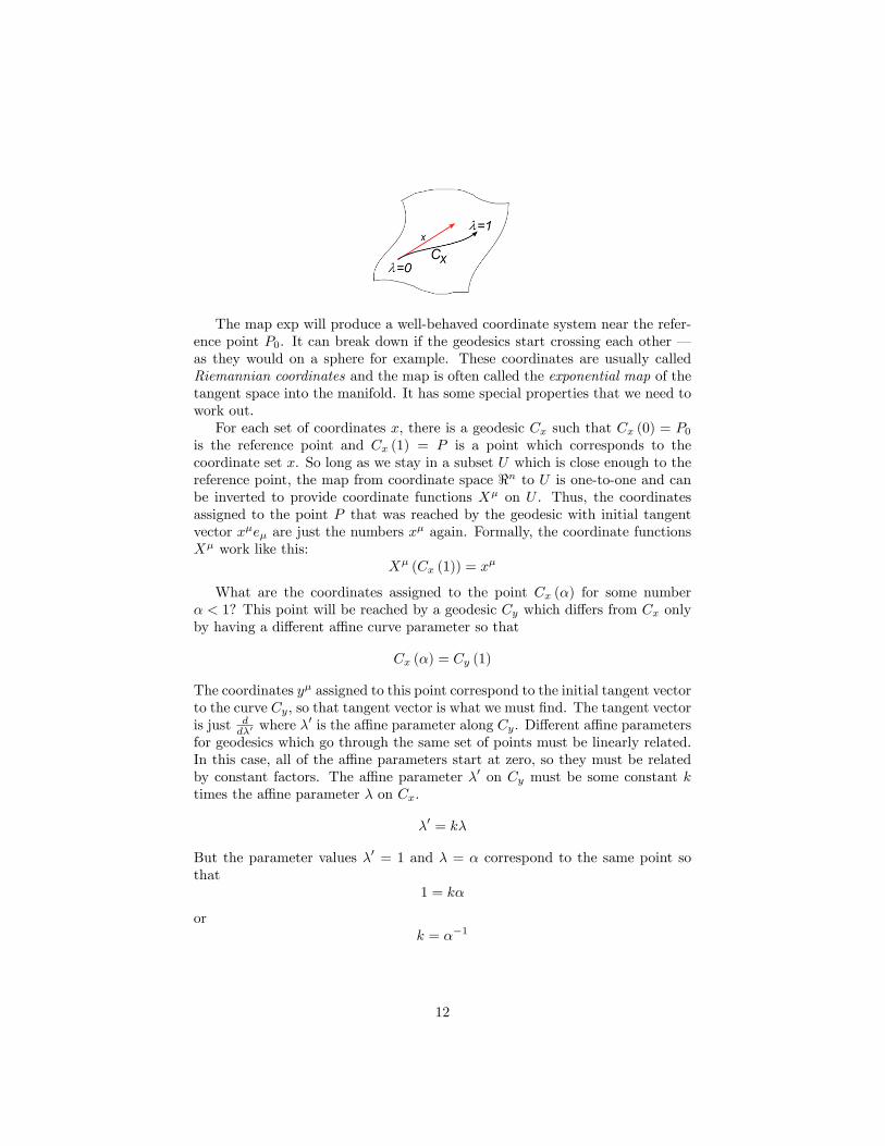
The map exp will produce a well-behaved coordinate system near the refer-ence point P0. It can break down if the geodesics start crossing each other �as they would on a sphere for example. These coordinates are usually calledRiemannian coordinates and the map is often called the exponential map of thetangent space into the manifold. It has some special properties that we need towork out.For each set of coordinates x, there is a geodesic Cx such that Cx (0) = P0

is the reference point and Cx (1) = P is a point which corresponds to thecoordinate set x. So long as we stay in a subset U which is close enough to thereference point, the map from coordinate space <n to U is one-to-one and canbe inverted to provide coordinate functions X� on U . Thus, the coordinatesassigned to the point P that was reached by the geodesic with initial tangentvector x�e� are just the numbers x� again. Formally, the coordinate functionsX� work like this:

X� (Cx (1)) = x�

What are the coordinates assigned to the point Cx (�) for some number� < 1? This point will be reached by a geodesic Cy which di¤ers from Cx onlyby having a di¤erent a¢ ne curve parameter so that

Cx (�) = Cy (1)

The coordinates y� assigned to this point correspond to the initial tangent vectorto the curve Cy, so that tangent vector is what we must �nd. The tangent vectoris just d

d�0 where �0 is the a¢ ne parameter along Cy. Di¤erent a¢ ne parameters

for geodesics which go through the same set of points must be linearly related.In this case, all of the a¢ ne parameters start at zero, so they must be relatedby constant factors. The a¢ ne parameter �0 on Cy must be some constant ktimes the a¢ ne parameter � on Cx.

�0 = k�

But the parameter values �0 = 1 and � = � correspond to the same point sothat

1 = k�

ork = ��1

12

and the a¢ ne parameter on Cy is just �0 = ��1�: Now �nd the tangent vector

to Cy.d

d�0= �

d

d�

or, in componentsy�e� = �x�e�

which yieldsy� = �x�

In terms of the coordinate functions and the curve Cx

X� (Cx (�)) = �x� = �X� (Cx (1))

For any geodesic through the reference point P0, the coordinate functionsare given by

X� (C (�)) = �X� (C (1))

In terms of the simpler notation x� (t) = X� (C (t)), this result implies that thecoordinates along any geodesic through P0 obey the relation

x� (t) = tx� (1) = tu�

where u� is the initial tangent vector.Now consider what the geodesic equation will look like in this coordinate

system. Let the functions x� (t) describe the coordinate image of a curve passingthrough the reference point. The tangent vector to this curve is given by

u =d

dt=dx�

dt@� = _x�e�

Now calculate for a bit:

ruu = ru (u�@�) = (ruu�) @� + u�ru@�

ruu = u (u�) @� + u�u�r@�@�

= ddtu

�@� + u�u�@��

���

= _u�@� + u�u�@��

���

= (�x� + u�u�����) @�

and �nd that the geodesic equation becomes

�x� + u�u����� = 0

But, in these coordinates,x� (t) = tx� (1)

so that�x� = 0

13

Putting this result back into the geodesic equation, we get the constraints

u�u����� (P0) = 0

for any values of the components u�.Split the connection into symmetric and antisymmetric parts:

���� = ��(��) + �

�[��]

and notice that, by antisymmetry

u�u���[��] = �u�u���[��]

and, by renaming dummy indexes,

u�u���[��] = �u�u���[��] = �u�u���[��]

so thatu�u���[��] = 0:

The antisymmetric part of the connection drops out of the constraints, leaving

u�u���(��) (P0) = 0

which can be satis�ed for all values of u� only if

��(��) (P0) = 0:

Thus, the symmetric part of the connection coe¢ cient array vanishes at thereference point of a Riemannian coordinate system.

4 Connection Tensors

4.1 Torsion

Consider how covariant derivatives commute when they act on a function.

[Du; Dv] f = DuDvf �DvDuf

ButDuDvf = rurvf �rruvf

and these derivatives of functions are just the vectors themselves acting as op-erators

DuDvf = uvf � (ruv) f= fuv �ruvg f

The commutator is then

[Du; Dv] f = fuv �ruvg f � fvu�rvug f= f[u; v]�ruv +rvug f

14

or, since f is an arbitrary function, the commutator is just a vector �eld.

[Du; Dv] = [u; v]�ruv +rvu:

The torsion is de�ned to be a third rank tensor �eld that yields the vector �eld

T (u; v) = � [Du; Dv]

= � [u; v] +ruv �rvu

for any vector �elds u; v.For future reference, note that the de�nition implies that the arguments u; v

of the torsion tensor are both di¤erentiating vector �elds. Thus, a derivativeoperation such as rwT (u; v) will treat T (u; v) as a simple vector �eld and willnot include counter terms for its arguments.In a holonomic frame, the components of the torsion tensor are

T ��� = dx� � T (e�; e�) = dx� ��re�e� �re�e�

�= ���� � ����

so the torsion is essentially the antisymmetric part of the connection coe¢ cientarray.The torsion is a tensor � it has to be because we constructed it from covari-

ant derivatives � and no coordinate transformation can ever make it vanish.As we have seen, the rest of the connection, the symmetric part, can be madeto vanish at a point by choosing Riemannian coordinates there.

4.2 De�nition of Curvature

Now consider how covariant derivatives commute when they act on a vector�eld. As we saw earlier, the object with the simplest properties is

R (u; v)w = [ru;rv]w �r[u;v]w:

Here, R is regarded as a linear operator on the vector �eld w. This de�nitionuses derivatives that do not treat the di¤erentiating vector �elds u; v as tensorarguments. Nevertheless, it produces a fourth-rank tensor. With all of itsarguments made explicit, this Riemannian Curvature tensor is

Riem (�;w; u; v) = � � R (u; v)w= � � [ru;rv]w � � � r[u;v]w

where � is a form and w; u; v are vectors. The components of this tensor canbe expressed in terms of the connection and commutation coe¢ cients as

R���� = re����� �re����� + �������� � �������� � c�������:

where the derivatives are regarded as acting on ordinary scalar �elds.

15

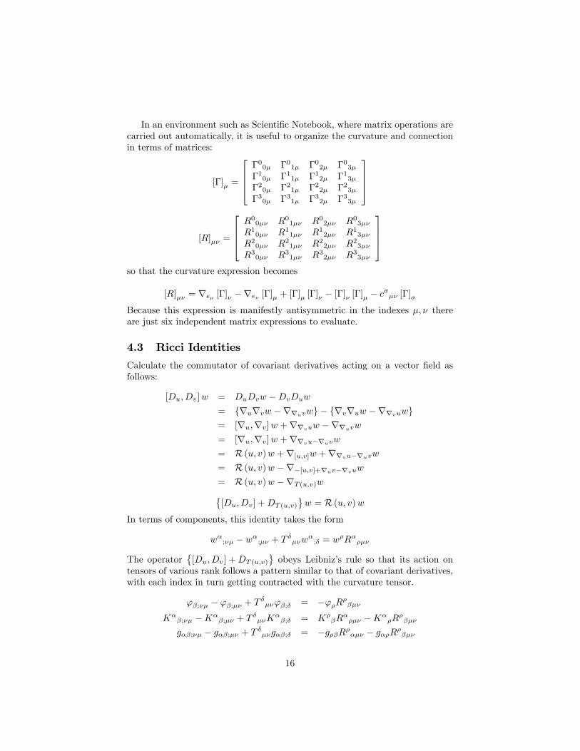
In an environment such as Scienti�c Notebook, where matrix operations arecarried out automatically, it is useful to organize the curvature and connectionin terms of matrices:

[�]� =

2664�00� �01� �02� �03��10� �11� �12� �13��20� �21� �22� �23��30� �31� �32� �33�

3775

[R]�� =

2664R00�� R01�� R02�� R03��R10�� R11�� R12�� R13��R20�� R21�� R22�� R23��R30�� R31�� R32�� R33��

3775so that the curvature expression becomes

[R]�� = re� [�]� �re� [�]� + [�]� [�]� � [�]� [�]� � c��� [�]�

Because this expression is manifestly antisymmetric in the indexes �; � thereare just six independent matrix expressions to evaluate.

4.3 Ricci Identities

Calculate the commutator of covariant derivatives acting on a vector �eld asfollows:

[Du; Dv]w = DuDvw �DvDuw

= frurvw �rruvwg � frvruw �rrvuwg= [ru;rv]w +rrvuw �rruvw

= [ru;rv]w +rrvu�ruvw

= R (u; v)w +r[u;v]w +rrvu�ruvw

= R (u; v)w �r�[u;v]+ruv�rvuw

= R (u; v)w �rT (u;v)w�[Du; Dv] +DT (u;v)

w = R (u; v)w

In terms of components, this identity takes the form

w�;�� � w�;�� + T ���w�;� = w�R����

The operator�[Du; Dv] +DT (u;v)

obeys Leibniz�s rule so that its action on

tensors of various rank follows a pattern similar to that of covariant derivatives,with each index in turn getting contracted with the curvature tensor.

'�;�� � '�;�� + T ���'�;� = �'�R����K�

�;�� �K��;�� + T

���K

��;� = K�

�R���� �K�

�R����

g��;�� � g��;�� + T ���g��;� = �g��R���� � g��R����

16

4.4 Bianchi Identities

4.4.1 Jacobi Identity

The fundamental consistency relation for any system of commutors is the Jacobiidentity

[[A;B] ; C] + [[C;A] ; B] + [[B;C] ; A] = 0

which can be veri�ed just by writing out the expression in terms of products �everything cancels. It does not matter what sort of objects are being commuted.So long as they obey an associative algebra (where factors can be regrouped),then the Jacobi identity must hold. Any time that a set of commutation relationsis given, the Jacobi identity needs to be true.

4.4.2 Torsion

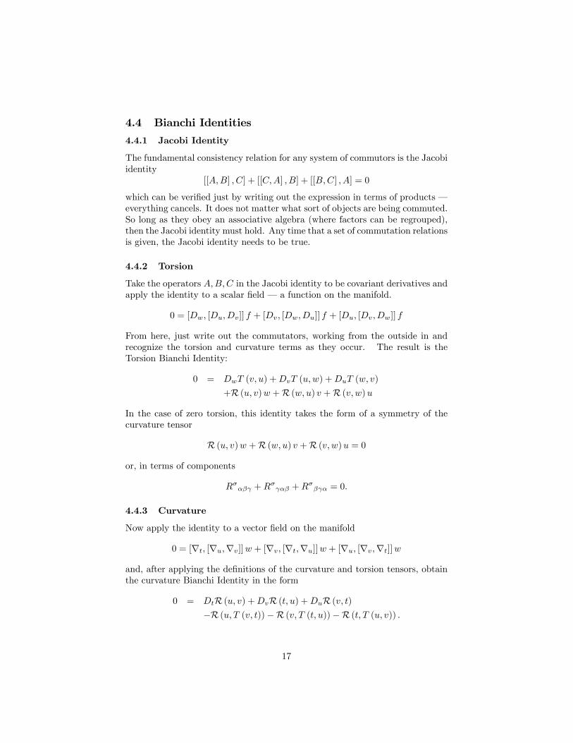
Take the operators A;B;C in the Jacobi identity to be covariant derivatives andapply the identity to a scalar �eld � a function on the manifold.

0 = [Dw; [Du; Dv]] f + [Dv; [Dw; Du]] f + [Du; [Dv; Dw]] f

From here, just write out the commutators, working from the outside in andrecognize the torsion and curvature terms as they occur. The result is theTorsion Bianchi Identity:

0 = DwT (v; u) +DvT (u;w) +DuT (w; v)

+R (u; v)w +R (w; u) v +R (v; w)u

In the case of zero torsion, this identity takes the form of a symmetry of thecurvature tensor

R (u; v)w +R (w; u) v +R (v; w)u = 0

or, in terms of components

R��� +R� �� +R

�� � = 0:

4.4.3 Curvature

Now apply the identity to a vector �eld on the manifold

0 = [rt; [ru;rv]]w + [rv; [rt;ru]]w + [ru; [rv;rt]]w

and, after applying the de�nitions of the curvature and torsion tensors, obtainthe curvature Bianchi Identity in the form

0 = DtR (u; v) +DvR (t; u) +DuR (v; t)�R (u; T (v; t))�R (v; T (t; u))�R (t; T (u; v)) :

17

In the case of zero torsion, this identity is a symmetry of the covariant derivativeof the curvature tensor

0 = DtR (u; v) +DvR (t; u) +DuR (v; t)

or, in terms of components

R����; +R�� �;� +R

��� ;� = 0

where the last three indexes are permuted cyclically from one term to the next.

4.5 Metric

In order to specify the lengths of vectors, and the angles between vectors, atensor g which eats pairs of vectors is needed � a second rank covariant tensor.Thus, the length of the vector v is given by

pg (v; v) while the angle � between

spacelike vectors u and v is given by cos � = g(u;v)pg(u;u)g(v;v)

. In the spacetime of

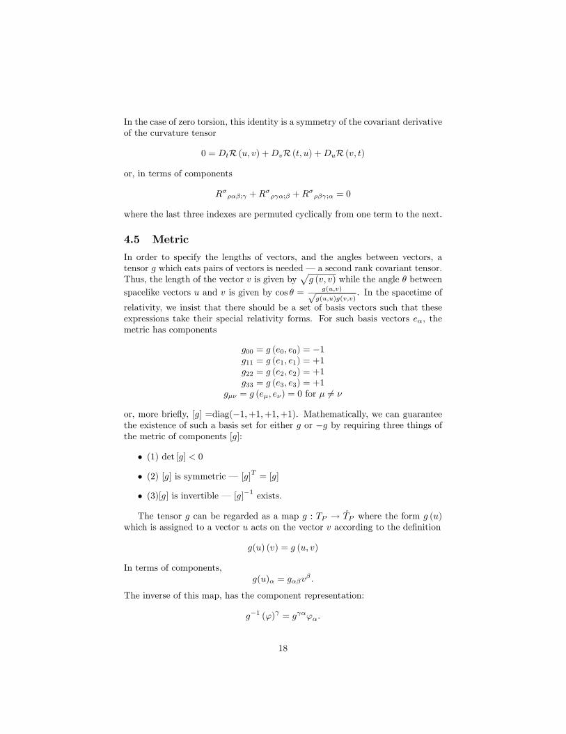
relativity, we insist that there should be a set of basis vectors such that theseexpressions take their special relativity forms. For such basis vectors e�, themetric has components

g00 = g (e0; e0) = �1g11 = g (e1; e1) = +1g22 = g (e2; e2) = +1g33 = g (e3; e3) = +1

g�� = g (e�; e�) = 0 for � 6= �

or, more brie�y, [g] =diag(�1;+1;+1;+1). Mathematically, we can guaranteethe existence of such a basis set for either g or �g by requiring three things ofthe metric of components [g]:

� (1) det [g] < 0

� (2) [g] is symmetric � [g]T= [g]

� (3)[g] is invertible � [g]�1 exists.

The tensor g can be regarded as a map g : TP ! T̂P where the form g (u)which is assigned to a vector u acts on the vector v according to the de�nition

g(u) (v) = g (u; v)

In terms of components,g(u)� = g��v

� :

The inverse of this map, has the component representation:

g�1 (') = g �'�:

18

Putting these last two expressions together, we �nd

g �g�� = � �

or, in terms of matrix arrays of components,�g�1

�[g] = I; !

�g�1

�= [g]

�1:

Now de�ne a second rank tensor which acts on pairs of forms according to

g�1 ('; ) = g�1 (') � = ' � g�1 ( ) :

This contravariant second rank tensor has the components

g�1�!� ; !�

�= g�1

�!��� !� = g��

Historically, the metric tensor �eld has been regarded as the fundamental�eld variable of general relativity with everything else derived from it. Thatpoint of view has changed radically during the last few years. It now looks as ifthe connection is the fundamental gravitational variable while the metric tensoris a derived quantity which is sometimes needed in order to describe interactionsbetween gravity and matter.

4.6 Diagonalization of the Metric

For a basis transformatione�0 = U�0

�e�

to yield an orthonormal basis, the coe¢ cients U�0� must obey the conditions

U�0�e� � U�0�e� = ��� =

8<: �1 for � = � = 01 for � = � 6= 00 for � 6= �

orU�0

�U�0�g�� = ���

In matrix notation, these conditions take the form

[U ] [g] [U ]T= [�]

Notice that these are not the same as the conditions on a similarity transforma-tion that diagonalizes the matrix [g]. A similarity transformation would takethe form A [g]A�1.If the original basis is already orthonormal, the condition on a basis change

to a new orthonormal set is

[U ] [�] [U ]T= [�]

In this case, the transformation

[e0] = [U ] [e]

is a Lorentz Transformation.

19

4.7 Metricity

The link between the metric tensor and the connection is the covariant derivativeof the metric tensor � the metricity tensor. For an arbitrary metric in anarbitrary connection, the metricity tensor is just

Q (�; �; v) = �Dvg�1 (�; �)

orQ�� = �De g

�� = �e g�� � g����� � g����� :I am de�ning the metricity in terms of the inverse metric tensor because thatturns out to be more useful in calculations of gravitational dynamics than theregular metric tensor. From matrix algebra, any derivative operator D actingon the inverse of a matrix yields

D�m�1� = �m�1 (Dm)m�1

so that an equivalent de�nition of metricity is

Q (a; b; v) = Dvg (a; b)

orQ�� = g��Q

�� g�� = De g�� = g��;

= e g�� � g����� � g����� Ordinarily, one requires the metricity tensor to vanish so that the covariant

derivatives of inner products obey Leibniz�s rule:

De (u � v) = De

�u�g��v

��

=�De u

��g��v

� + u�Q�� v� + u�g��

�De v

��

The metricity amounts to the covariant derivative of the �dot�. A connectionfor which the metricity tensor vanishes is called a �metric compatible connec-tion�. This condition is usually interpreted as a constraint on the connectioncoe¢ cients:

e g�� = g����� + g���

��

I will follow the usual interpretation for a while and get expressions for theconnection coe¢ cients in terms of the metric. However, before we mess up thisexpression any further, notice that it is a beautifully simple system of linear �rstorder di¤erential equations in the metric components. Given the connectioncoe¢ cients, we can recover the metric tensor by solving this system of linearequations.The standard approach de�nes the object

��� = g�����

and notices that we already know that the torsion tensor is given by

T�� = g��c�� � 2��[� ]

20

so that��[� ] =

1

2(g��c

�� � T�� )

The metric compatibility condition takes the form

e g�� = ��� + ���

or�(��) =

1

2e g�� :

This system of linear equations can be solved for the connection coe¢ cients.The system to be solved is

�(��) =1

2b�� ; ��[� ] =

1

2a��

or, equivalently��� + ��� = b�� ��� � �� � = a��

Cyclically permute the argments of this last equation and write it as

��� = �� � + a��

which can be substituted into the �rst equation of the pair

��� + �� � + a�� = b��

and gives the key result:

��� + �� � = b�� � a�� :

Now denote cyclic index permutations by

(C�)�� = �� �

andB�� = b�� � a��

so that the equation that we have to solve becomes just

� + C� = B:

Operate on it twice with the cyclic permutation operator

C� + C2� = CB

C2� + � = C2B:

Now we have three equations in the three unknowns �; C�; C2�.

21

Eliminate C2� using the last equation

C2� = C2B � �:

Next, eliminate C� by using middle equation

C� = CB � C2� = CB � C2B + �:

The remaining equation them becomes

� + CB � C2B + � = B

or2� = C2B � CB +B

� =1

2

�C2B � CB +B

���� =

1

2(B �� �B� � +B�� )

Now unravel the de�nitions

B�� = b�� � a�� = e g�� � g��c�� + T��

and get the �nal expression for the connection coe¢ cients in terms of the metricand torsion tensors.

��� =12g�� (e g�� � g��c�� + T��

+e�g � � g��c� � + T� � � e�g� + g �c��� � T ��)In the case of a holonomic frame and zero torsion, this expression reduces tojust a combination of derivatives of the metric tensor components.

��� =1

2g�� (e g�� + e�g � � e�g� )

4.8 Curvature-Metricity Identity

Let the curvature operator act on the metric tensor�[Du; Dv] +DT (u;v)

g (a; b) = �g (R (u; v) a; b)� g (a;R (u; v) b)

or

DuDvg (a; b)�DvDug (a; b)+DT (u;v)g (a; b) = �g (R (u; v) a; b)�g (R (u; v) b; a)

which, from the de�nition of metricity yields

DuQ (a; b; v)�DvQ (a; b; u)+Q (a; b; T (u; v)) = �g (R (u; v) a; b)�g (R (u; v) b; a)

or, in terms of indexes,

Q���;� �Q���;� +Q���T ��� = �R���� �R����which connects the metricity to the curvature tensor. When the metricity is zero,this identity becomes an additional index symmetry of the curvature tensor

R���� = �R����

22

4.9 Index Symmetries of the Curvature Tensor

From its de�nition, the curvature tensor obeys

R���� = �R���� :

In the most general case, this is the only symmetry which the tensor has. Countits components in a four dimensional space: Array its independent componentsin rows according to the last two indexes and columns according to the �rsttwo. That makes six independent rows and sixteen independent columns for atotal of 96 independent components.In the most common case, the connection is metric compatible, which, from

the curvature-metricity identity, guarantees antisymmetry in the �rst two in-dexes. The array now has just six columns and six rows and the curvature has36 independent components.If, in addition to being metric compatible, the connection is torsion-free,

then the torsion Bianchi identities put additional constraints on the curvaturecomponents:

R��� +R� �� +R

�� � = 0

These additional 16 equations reduce the number of components to just 20.Lower an index in the torsion Bianchi identities and start manipulating them,

along with the antisymmetries in the �rst two and second two indexes:

R��� +R� �� +R�� � = 0 (1)

symmetrize on �; � to so that the �rst term vanishes and the remaing two yield

R� �� +R� �� +R�� � +R�� � = 0

or, re-grouping the �rst term with the last and the second with the third,

(R� �� +R�� �) + (R� �� +R�� �) = 0

and using the antisymmetry of the �rst and second pairs of curvature indexes

(R�� � �R ���) + (R�� � �R ���) = 0 (2)

Now symmetrize equation(1) on �; � so that the last term vanishes

R��� +R��� +R� �� +R� �� = 0

or(R��� �R� ��) + (R��� �R� ��) = 0 (3)

Then symmetrize equation (1) on ; � so that the middle term vanishes

R��� +R ��� +R�� � +R ��� = 0

or(R��� �R� ��) + (R ��� �R�� �) = 0 (4)

23

The three equations (2,3,4) have the form

z + x = 0y + z = 0x+ y = 0

where x; y; z are the tensor combinations in parentheses. The solution to thissystem is easily seen to be x = y = z = 0 so that we obtain the index symmetry

R�� � = R ��� :

Notice that this last index symmetry is derived from the torsion Bianchiidentities for zero torsion. It does not contain quite all of the information whichis in those identities, however. One way to see this is to count the independentcomponents of the Riemann tensor again, using this index symmetry. Think ofthe array of components as having rows and columns labeled by antisymmetrizedindex pairs. That makes it a six by six array. The last index symmetry makesthat array symmetric which means that it has 6�72 independent components �21. Since we know from counting the torsion Bianchi identities that there areonly 20 independent components, there is evidently one constraint that is notcaptured by any of the index symmetries.To see what the remaining constraint is, notice that we symmetrized various

indexes with the one �xed index in the torsion identity. That procedure wouldmiss whatever constraint is gotten by antisymmetrizing those indexes. Since thetorsion bianchi identities are already antisymmetric in three indexes and havethe form

R�[�� ] = 0

the only possible result of antisymmetrizing the remaining �xed index � withany other index is the totally antisymmetrized expression

R[��� ] = 0:

The one component of the curvature tensor that is permitted by the indexsymmetries but forbidden by this remaining constraint is

R��� = �"���

where � is an arbitrary function and "��� is the totally antisymmetric Levi-civita symbol. The missing constraint is that this totally antisymmetric com-ponent of the Riemann tensor must be zero.

"��� R��� = 0:

24