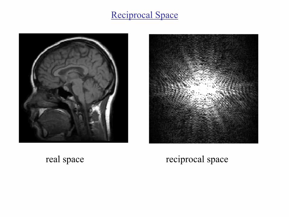
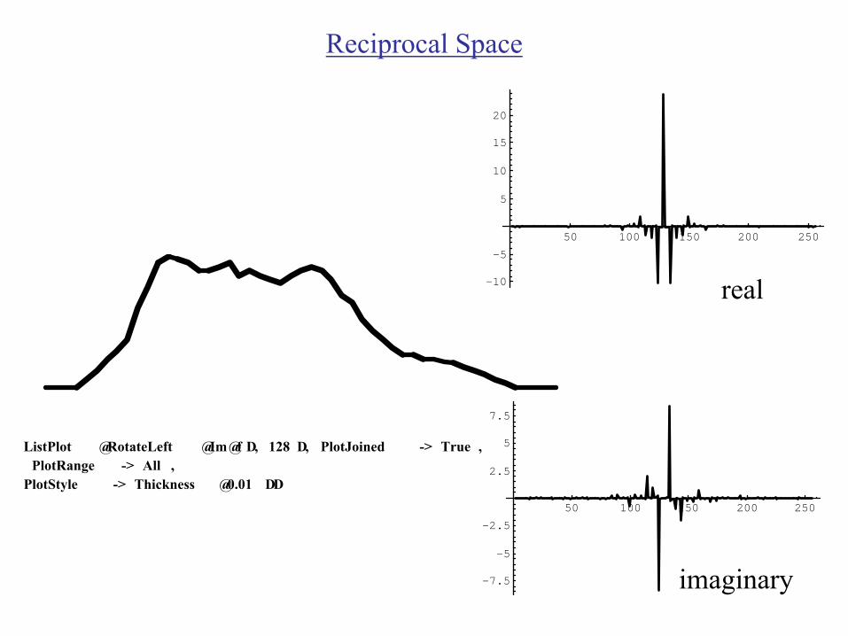
Reciprocal Space

Fourier Transforms

Outline • Introduction to reciprocal space • Fourier transformation • Some simple functions • Area and zero frequency components • 2- dimensions • Separable • Central slice theorem • Spatial frequencies • Filtering • Modulation Transfer Function

Reciprocal Space

real space reciprocal space

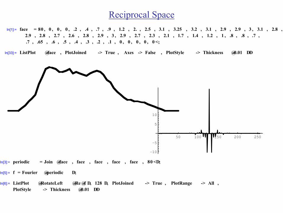
Reciprocal Space In[1]:= face = 80 , 0 , 0 , 0 , .2 , .4 , .7 , .9 , 1.2 , 2. , 2.5 , 3.1 , 3.25 , 3.2 , 3.1 , 2.9 , 2.9 , 3 , 3.1 , 2.8 ,

2.9 , 2.8 , 2.7 , 2.6 , 2.8 , 2.9 , 3 , 2.9 , 2.7 , 2.3 , 2.1 , 1.7 , 1.4 , 1.2 , 1 , .8 , .8 , .7 , .7 , .65 , .6 , .5 , .4 , .3 , .2 , .1 , 0 , 0 , 0 , 0 , 0 <;

In[33]:= ListPlot @face , PlotJoined -> True , Axes -> False , PlotStyle -> Thickness @0.01 DD

50 100 150 200 250

-10

-5

5

10

In[3]:= periodic = Join @face , face , face , face , face , 80 <D;

In[5]:= f = Fourier @periodic D;

In[6]:= ListPlot @RotateLeft @Re @f D, 128 D, PlotJoined -> True , PlotRange -> All , PlotStyle -> Thickness @0.01 DD

Reciprocal Space

50 100 150 200 250

-10

-5

5

10

15

20

real

ListPlot @RotateLeft @Im@f D, 128 D, PlotJoined -> True , PlotRange -> All ,

PlotStyle -> Thickness @0.01 DD 50 100 150 200 250

-7.5

-5

-2.5

2.5

5

7.5

imaginary

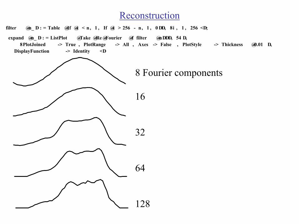
Reconstruction filter @n_ D : = Table @If @i < n, 1 , If @i > 256 - n , 1 , 0 DD, 8i , 1 , 256 <D;

expand @n_ D : = ListPlot @Take @Re @Fourier @f filter @nDDD, 54 D, 8PlotJoined -> True , PlotRange -> All , Axes -> False , PlotStyle -> Thickness @0.01 D,

DisplayFunction -> Identity <D

8 Fourier components

16

32

64

128

Fourier Transforms

For a complete story see: Brigham “Fast Fourier Transform”

Here we want to cover the practical aspects of Fourier Transforms.

Define the Fourier Transform as: ∞

G(k) = ℑ{g(x)}= ∫ g(x)e−ikxdx −∞

There are slight variations on this definition (factors of π and the sign in the exponent), we will revisit these latter, i=√-1.

Also recall that e−ikx = cos(kx) − i sin(kx)

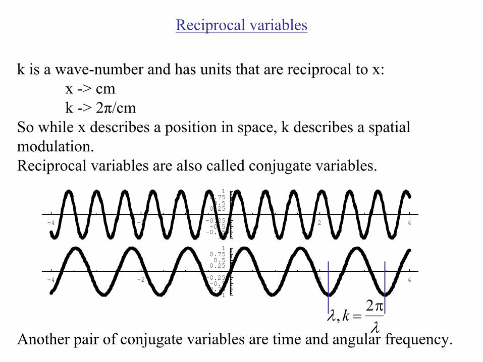
Reciprocal variables

k is a wave-number and has units that are reciprocal to x: x -> cm k -> 2π/cm

So while x describes a position in space, k describes a spatial modulation. Reciprocal variables are also called conjugate variables.

-4 -2 2 4

-1 -0.75 -0.5

-0.25

0.25 0.5

0.75 1

-4 -2 2 4

-1 -0.75 -0.5

-0.25

0.25 0.5

0.75 1

2 πλ, k =λ

Another pair of conjugate variables are time and angular frequency.

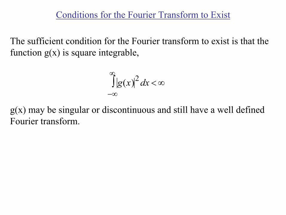
Conditions for the Fourier Transform to Exist

The sufficient condition for the Fourier transform to exist is that the function g(x) is square integrable,

∞ ∫ g(x)2 dx < ∞

−∞

g(x) may be singular or discontinuous and still have a well defined Fourier transform.

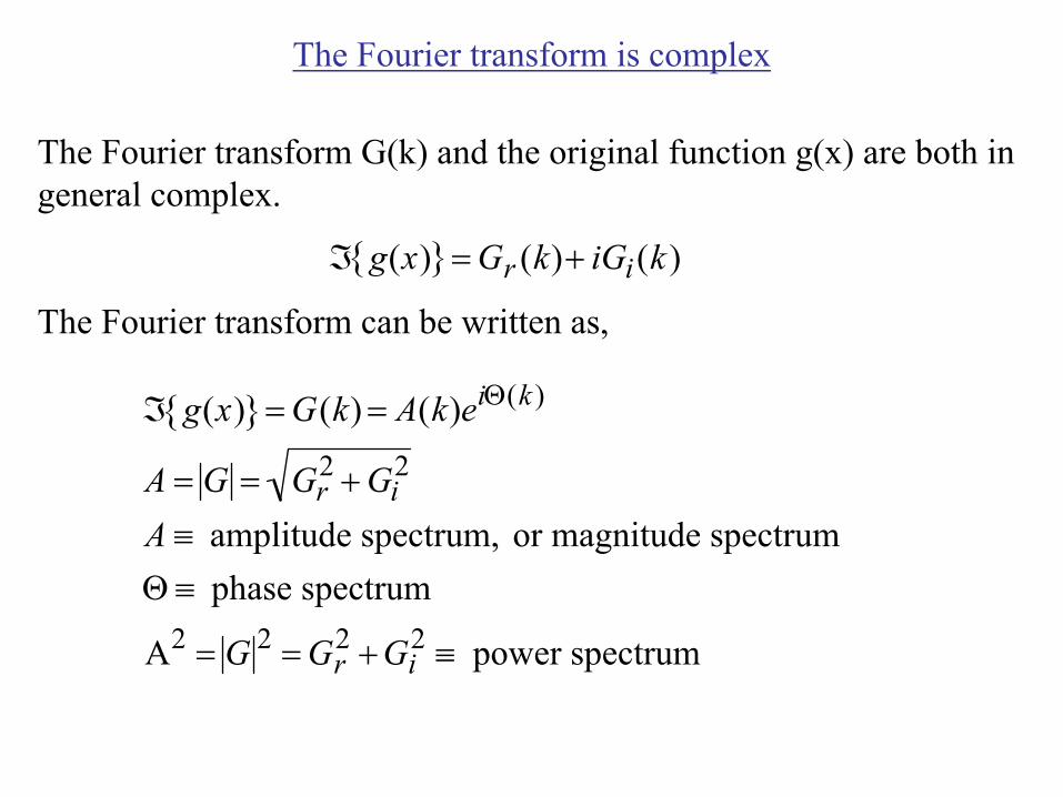
The Fourier transform is complex

The Fourier transform G(k) and the original function g(x) are both in general complex.

ℑ{g(x)}= Gr (k)+ iGi (k )

The Fourier transform can be written as,

ℑ{g(x)}= G(k) = A(k)eiΘ(k )

A = G = Gr 2 + Gi

2

A ≡ amplitude spectrum, or magnitude spectrum

Θ ≡ phase spectrum

A2 = G 2 = Gr 2 + Gi

2 ≡ power spectrum

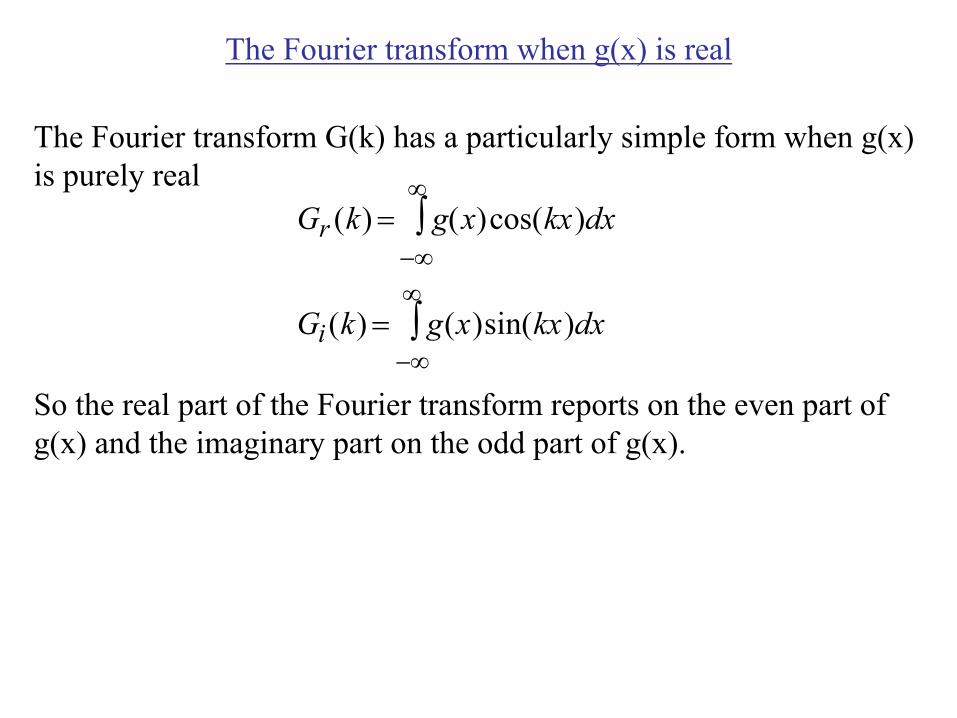
The Fourier transform when g(x) is real

The Fourier transform G(k) has a particularly simple form when g(x) is purely real ∞

Gr (k) = ∫ g(x)cos(kx)dx −∞ ∞

Gi (k) = ∫ g(x)sin(kx)dx −∞

So the real part of the Fourier transform reports on the even part of g(x) and the imaginary part on the odd part of g(x).

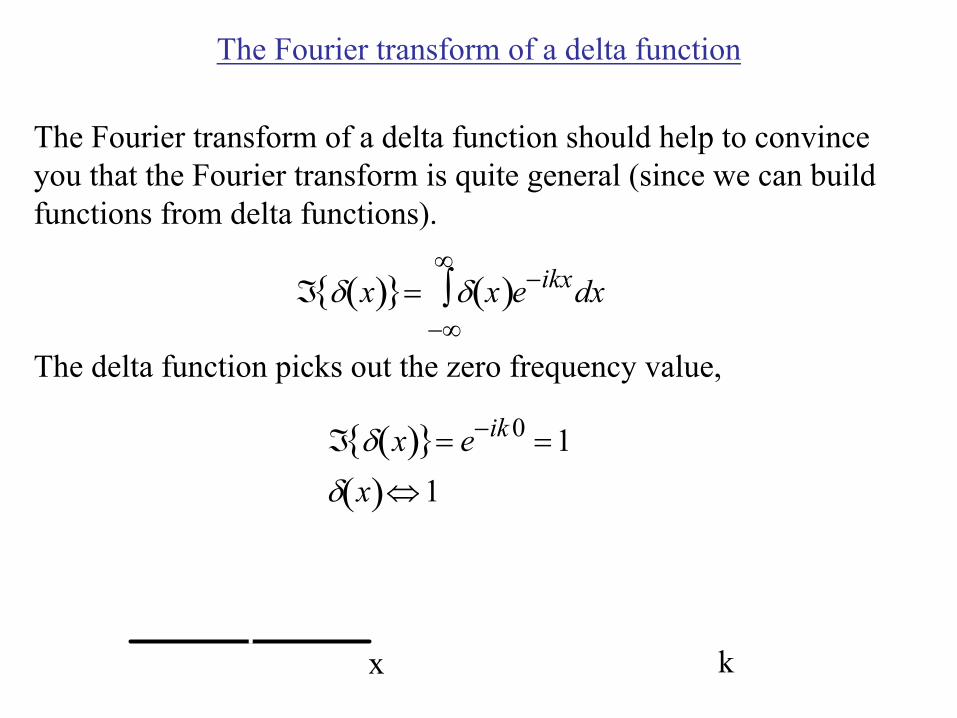
The Fourier transform of a delta function

The Fourier transform of a delta function should help to convince you that the Fourier transform is quite general (since we can build functions from delta functions).

∞ ( )}= ∫ δ xℑ{δ x ( )e−ikxdx

−∞

The delta function picks out the zero frequency value,

ℑ{δ(x)}= e−ik 0 = 1 δ x( )⇔ 1

x k

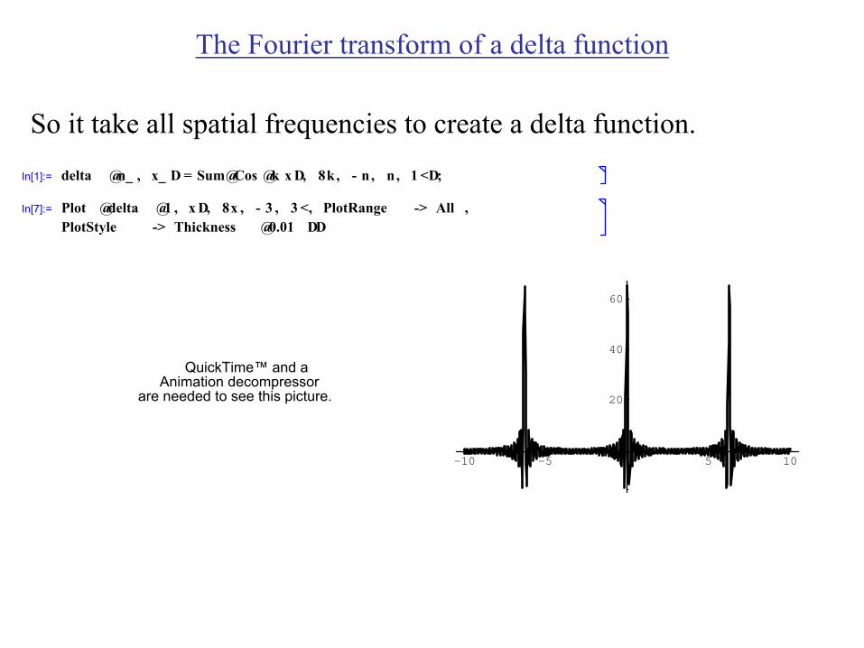
The Fourier transform of a delta function

So it take all spatial frequencies to create a delta function. In[1]:= delta @n_ , x_ D = Sum@Cos @k x D, 8k, - n , n , 1 <D;

In[7]:= Plot @delta @1 , x D, 8x , - 3 , 3 <, PlotRange -> All , PlotStyle -> Thickness @0.01 DD

QuickTime™ and aAnimation decompressor

are needed to see this picture.

-10 -5 5 10

20

40

60

The Fourier transform

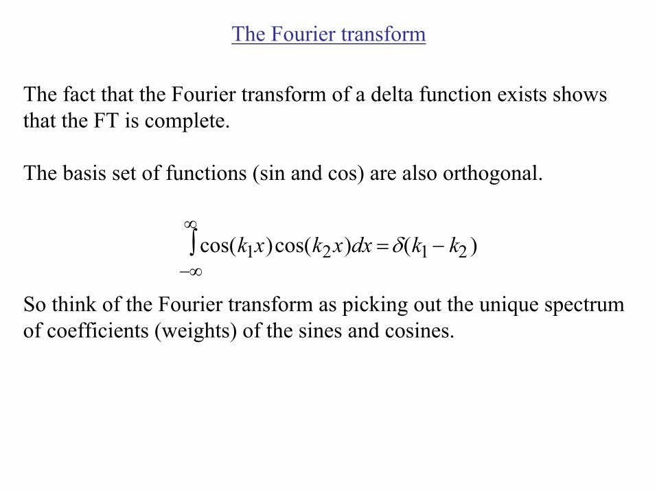
The fact that the Fourier transform of a delta function exists shows that the FT is complete.

The basis set of functions (sin and cos) are also orthogonal.

∞ ∫ cos(k1x)cos(k2 x)dx =δ(k1 − k2 )

−∞

So think of the Fourier transform as picking out the unique spectrum of coefficients (weights) of the sines and cosines.

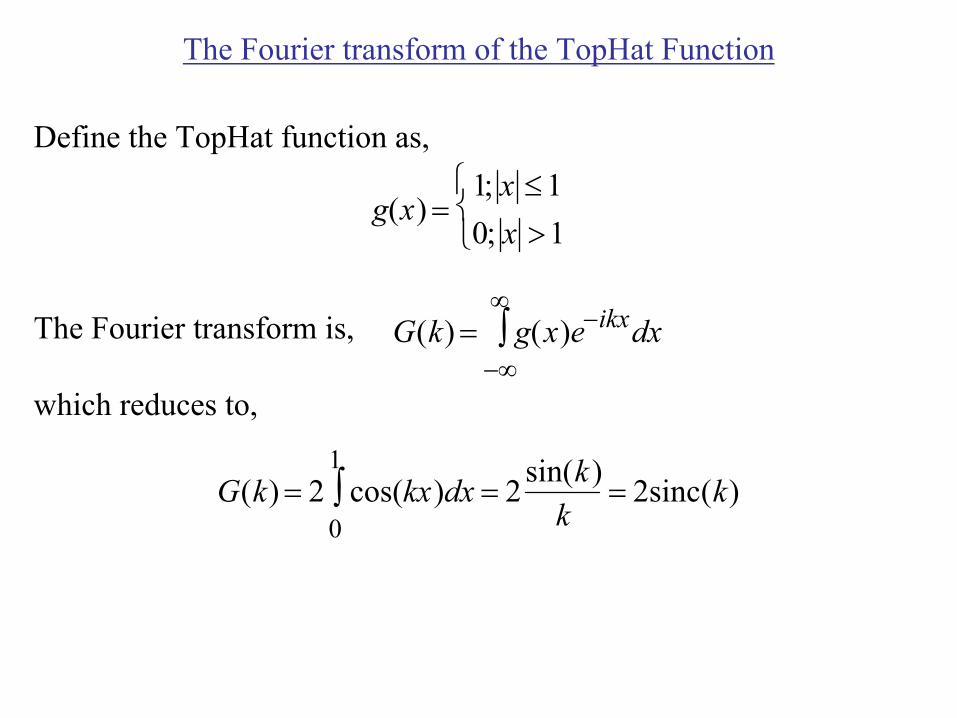
The Fourier transform of the TopHat Function

Define the TopHat function as, 1; x ≤ 1

g(x) = 0; x > 1

∞ The Fourier transform is, G(k) = ∫ g(x)e−ikxdx

−∞

which reduces to,

1 G(k) = 2 ∫ cos(kx)dx = 2sin(k )

= 2sinc(k) 0 k

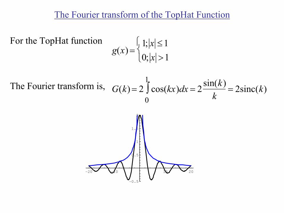
The Fourier transform of the TopHat Function

For the TopHat function 1; x ≤ 1 g(x) =

0; x > 1

1The Fourier transform is, G(k) = 2 ∫ cos(kx)dx= 2sin(k )

= 2sinc(k) 0 k

-20 -10 10 20

-0.5

0.5

1

1.5

2

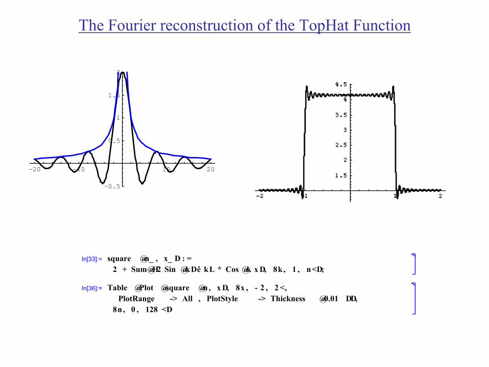
The Fourier reconstruction of the TopHat Function

-20 -10 10 20

-0.5

0.5

1

1.5

2

In[33]:= square @n_ , x_ D : = 2 + Sum@H2 Sin @kDê kL * Cos @k x D, 8k, 1 , n<D;

In[36]:= Table @Plot @square @n, x D, 8x , - 2 , 2 <, PlotRange -> All , PlotStyle -> Thickness @0.01 DD,

8n , 0 , 128 <D

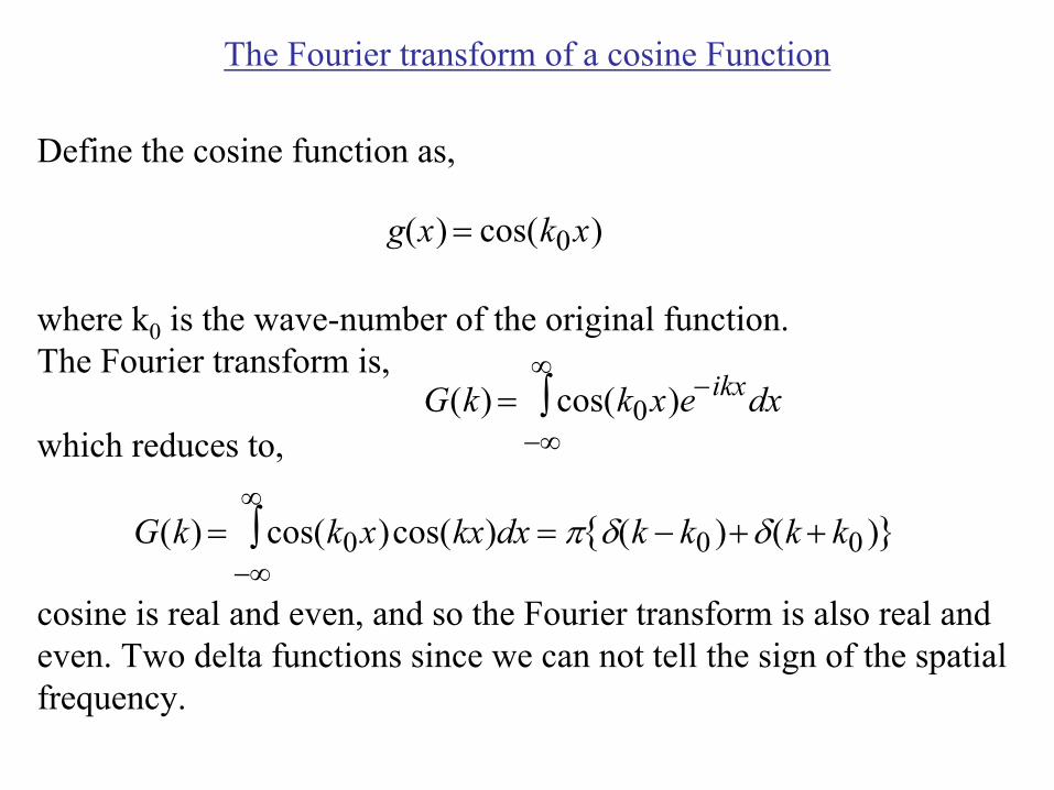
The Fourier transform of a cosine Function

Define the cosine function as,

g(x) = cos(k0 x)

where k0 is the wave-number of the original function. The Fourier transform is, ∞

G(k) = cos(k0 x)e−ikxdx∫which reduces to, −∞

∞ ∫ = π δ(k − k0 ) +δ(k + k0 )}{G(k) = cos(k0 x)cos(kx)dx

−∞

cosine is real and even, and so the Fourier transform is also real and even. Two delta functions since we can not tell the sign of the spatial frequency.

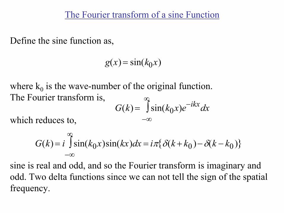
The Fourier transform of a sine Function

Define the sine function as,

g(x) = sin(k0 x)

where k0 is the wave-number of the original function. The Fourier transform is, ∞

G(k) = sin(k0 x)e−ikxdx∫which reduces to, −∞

∞ {∫ = iπ δ(k + k0 ) −δ(k − k0 )}G(k) = i sin(k0 x)sin(kx)dx

−∞

sine is real and odd, and so the Fourier transform is imaginary and odd. Two delta functions since we can not tell the sign of the spatial frequency.

Telling the sense of rotation

Looking at a cosine or sine alone one can not tell the sense of rotation (only the frequency) but if you have both then the sign is measurable.

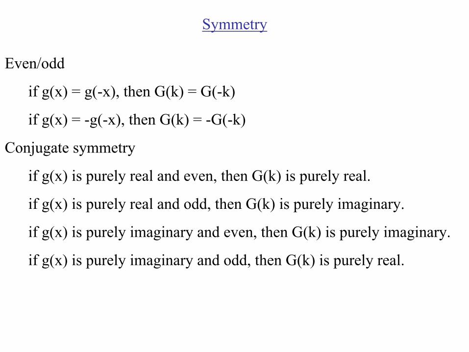
Symmetry

Even/odd

if g(x) = g(-x), then G(k) = G(-k)

if g(x) = -g(-x), then G(k) = -G(-k)

Conjugate symmetry

if g(x) is purely real and even, then G(k) is purely real.

if g(x) is purely real and odd, then G(k) is purely imaginary.

if g(x) is purely imaginary and even, then G(k) is purely imaginary.

if g(x) is purely imaginary and odd, then G(k) is purely real.

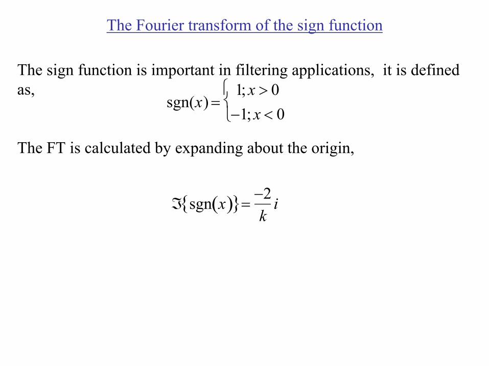
The Fourier transform of the sign function

The sign function is important in filtering applications, it is defined as, 1; x > 0

sgn(x) = −1; x < 0

The FT is calculated by expanding about the origin,

ℑ{sgn x( )}= − k 2 i

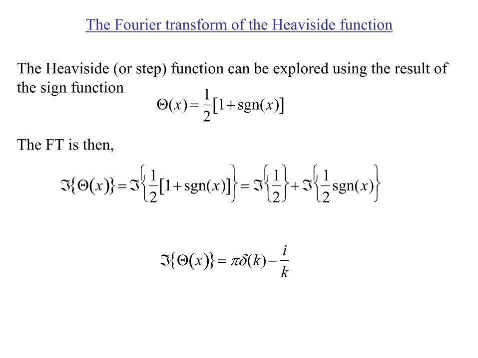
The Fourier transform of the Heaviside function

The Heaviside (or step) function can be explored using the result of the sign function 1

Θ(x) = 2

[1+ sgn(x)]

The FT is then,

{ ( )}= ℑ1 2

2

sgn(x)ℑ Θ x 2

[1 + sgn(x)]

= ℑ1

+ ℑ1

ℑ Θ x{ ( )}= πδ(k) − i k

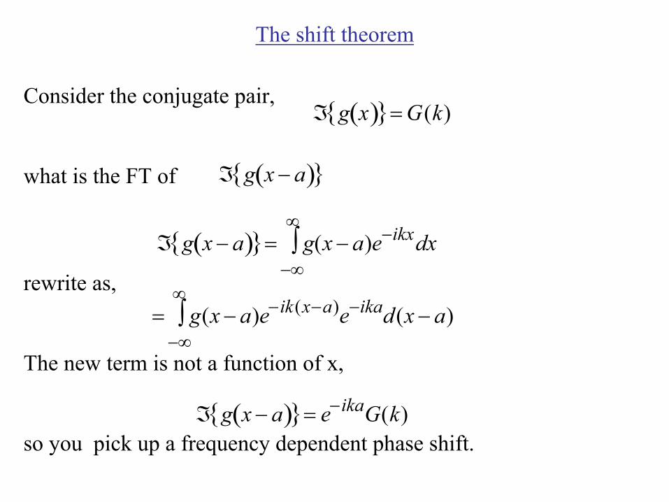
The shift theorem

Consider the conjugate pair, ℑ{g(x)}= G(k)

what is the FT of ℑ{g(x − a)}

∞ ℑ{g x − a)}= ∫ g(x − a)e−ikxdx(

−∞rewrite as, ∞

= ∫ g(x − a)e−ik(x−a)e−ikad(x − a) −∞

The new term is not a function of x,

ℑ{g x − a)}= e−ikaG(k)(so you pick up a frequency dependent phase shift.

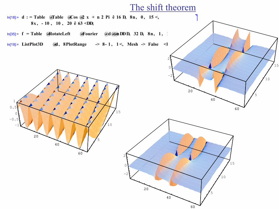
The shift theoremIn[18]:= d : = Table @Table @Cos @2 x + n 2 Pi ê 16 D, 8n, 0 , 15 <,

8x , - 10 , 10 , 20 ê 63 <DD;

In[35]:= f = Table @RotateLeft @Fourier @d@@nDDD, 32 D, 8n, 1 , 16 <D;

In[19]:= ListPlot3D @d, 8PlotRange -> 8- 1 , 1 <, Mesh -> False <D

20

40

60

5

10

15

-1

-0.5

0

0.5

1

20

40

60

20

40

60

5

10

15

-2

0

2

20

40

60

20

40

60

5

10

15

-2

0

2

20

40

60

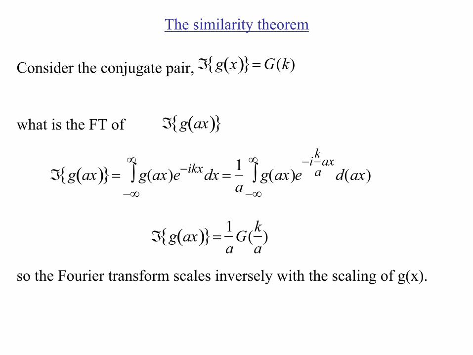
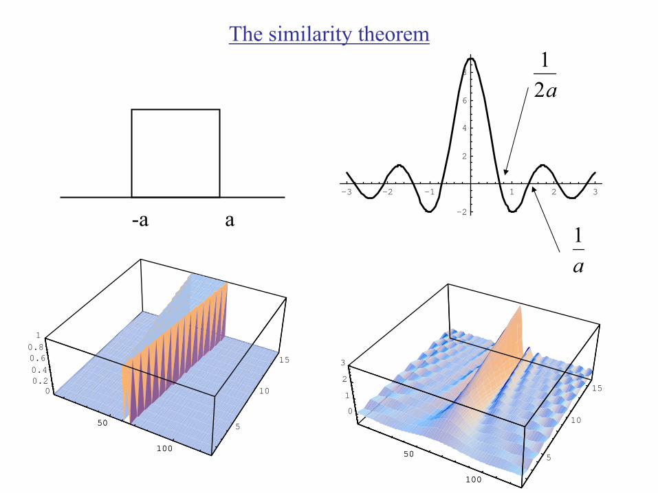
The similarity theorem

Consider the conjugate pair, ℑ{g(x)}= G(k)

what is the FT of ℑ{g(ax)}

∞ ℑ{g ax a( )}= ∫ g(ax)e−ikxdx =

1 ∞∫ g(ax)e

−i kaxd(ax)

−∞ a −∞

ℑ{g ax( )}= 1 G(

ak )

a

so the Fourier transform scales inversely with the scaling of g(x).

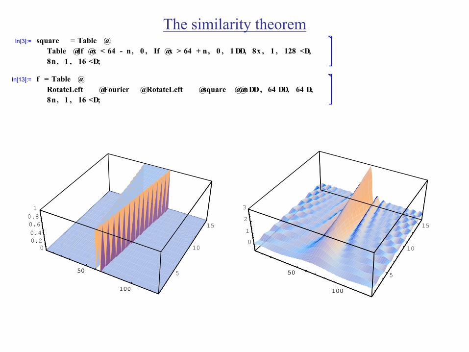
The similarity theoremIn[3]:= square = Table @

Table @If @x < 64 - n , 0 , If @x > 64 + n, 0 , 1 DD, 8x , 1 , 128 <D,8n, 1 , 16 <D;

In[13]:= f = Table @RotateLeft @Fourier @RotateLeft @square @@nDD, 64 DD, 64 D,8n, 1 , 16 <D;

50

100

5

10

15

00.20.40.60.81

50

100

50

100

5

10

15

0

1

2

3

50

100

The similarity theorem

50

100

5

10

15

00.20.40.60.81

50

10050

100

5

10

15

0

1

2

3

50

100

-3 -2 -1 1 2 3

-2

2

4

6

8

a-a

12a

1a

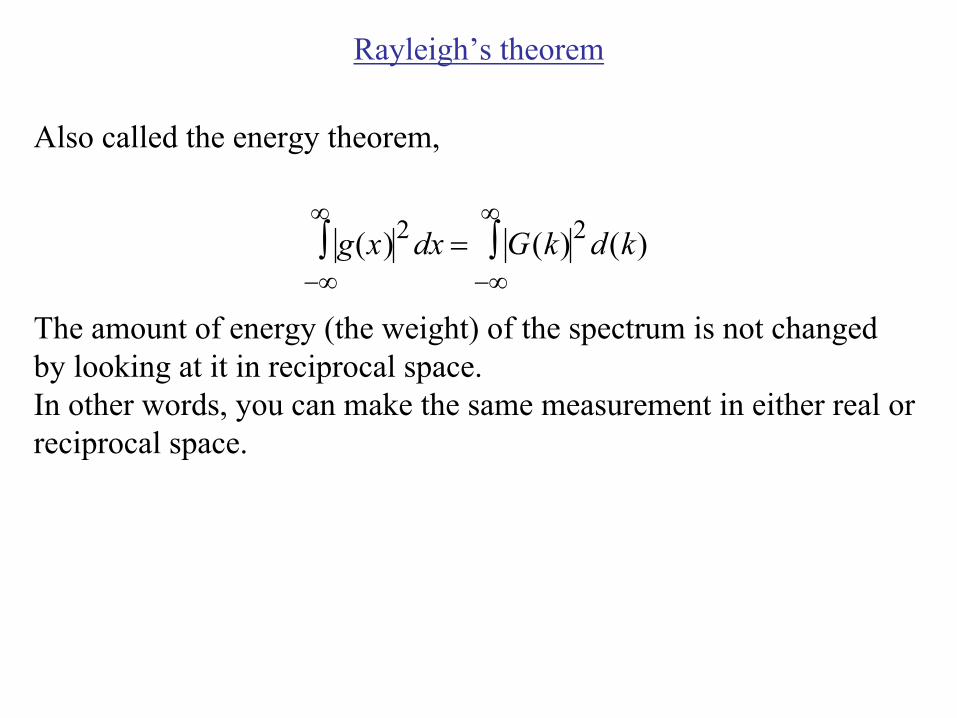
Rayleigh’s theorem

Also called the energy theorem,

∞ ∫ = G(k)2 d (k)g(x)2 dx

∞∫

−∞ −∞

The amount of energy (the weight) of the spectrum is not changedby looking at it in reciprocal space.In other words, you can make the same measurement in either real or reciprocal space.

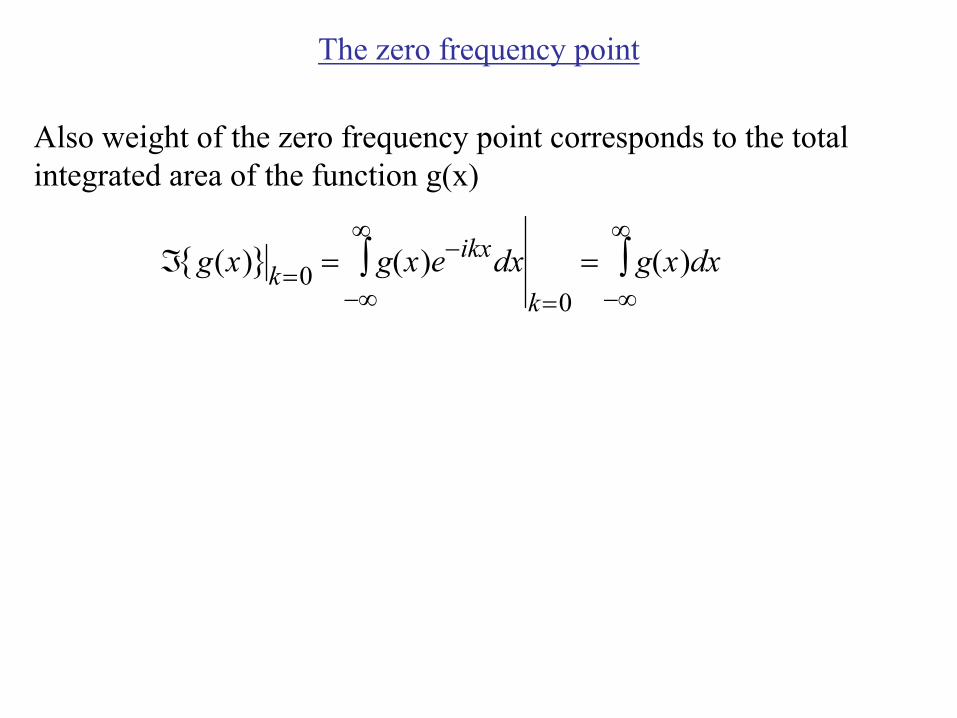
The zero frequency point

Also weight of the zero frequency point corresponds to the total integrated area of the function g(x)

∞∫

∞∫g(x)e−ikxdx=ℑ{g(x)}k =0 = g(x)dx

−∞ −∞k =0

4 3

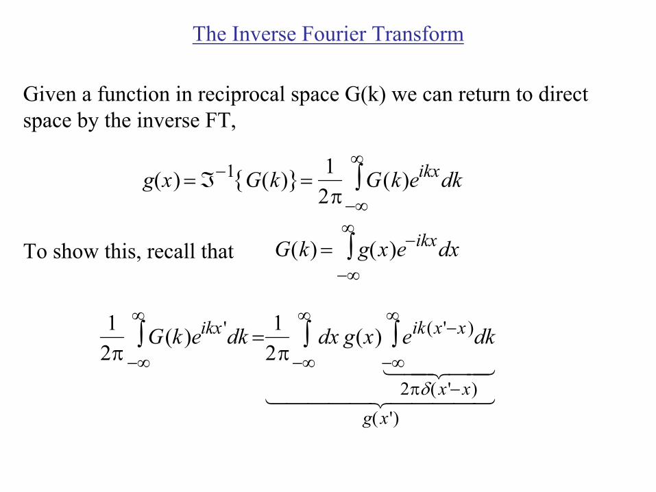
The Inverse Fourier Transform

Given a function in reciprocal space G(k) we can return to direct space by the inverse FT,

g(x) = ℑ−1{G(k)}= 1 ∞

G(k)eikxdk∫2 π −∞

∞ To show this, recall that G(k) = ∫ g( x)e−ikxdx

−∞

∞ ∞1 ∞∫ G(k )eikx ' dk =

1 ∫ dx g(x) ∫ eik(x'−x )dk2π −∞ 2π −∞ −∞1 4244

2πδ( x '− x)14444244443 g( x ')

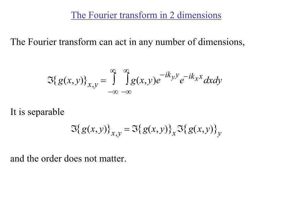
The Fourier transform in 2 dimensions

The Fourier transform can act in any number of dimensions,

∞ ∫ g(x, y)e −ikyye−ikxxdxdy

∞∫ℑ{g(x, y)}x,y =

−∞ −∞

It is separable

ℑ{g(x, y)}x,y = ℑ{g(x, y)}x ℑ{g(x, y)}y

and the order does not matter.

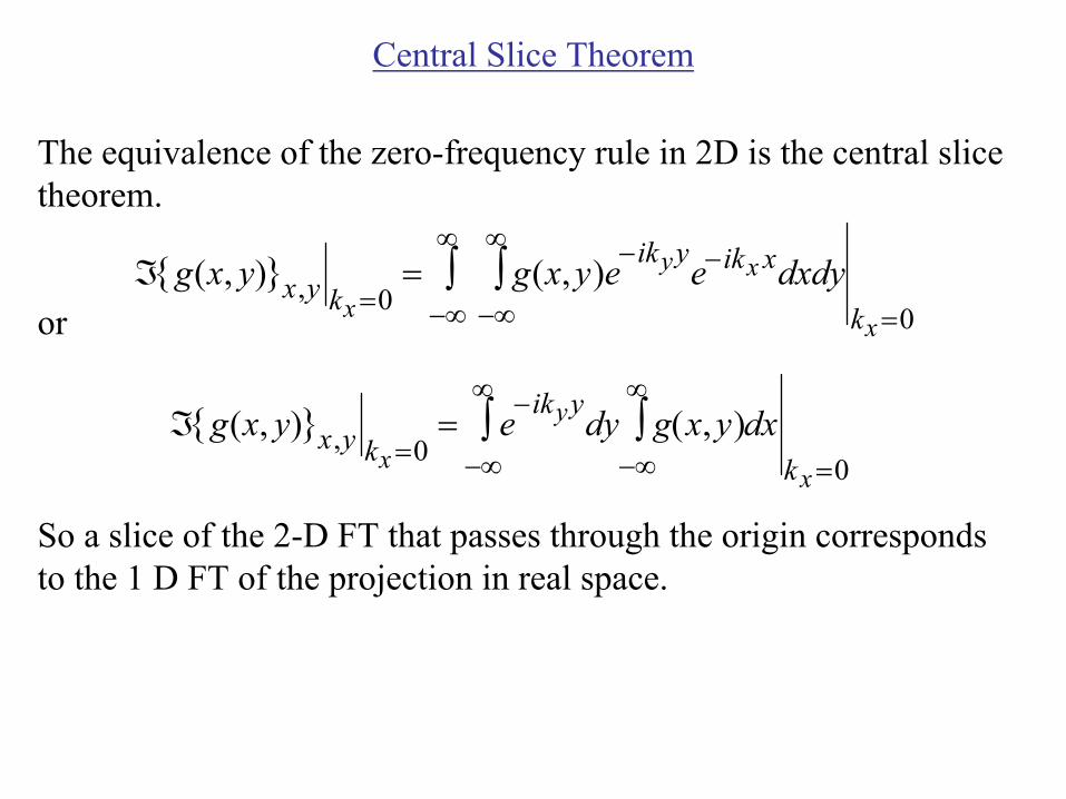
Central Slice Theorem

The equivalence of the zero-frequency rule in 2D is the central slice theorem.

∞ ∫ g(x, y)e −ikyye−ikx xdxdy

∞∫ℑ{g(x, y)}x,y kx =0

=−∞ −∞ kx =0or

∞ ∫ dy g(x, y)dx

∞∫−ikyy

= eℑ{g(x, y)}x,y kx =0 −∞ −∞ kx =0

So a slice of the 2-D FT that passes through the origin corresponds to the 1 D FT of the projection in real space.

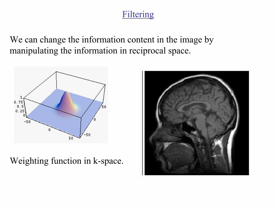
Filtering

We can change the information content in the image by manipulating the information in reciprocal space.

Weighting function in k-space.

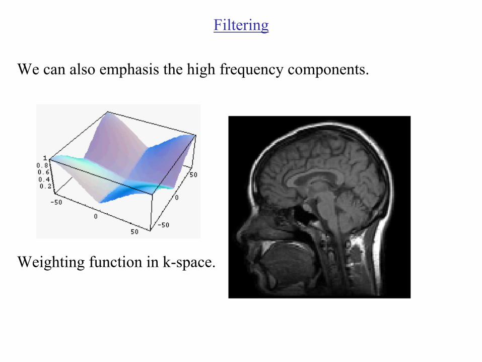
Filtering

We can also emphasis the high frequency components.

Weighting function in k-space.

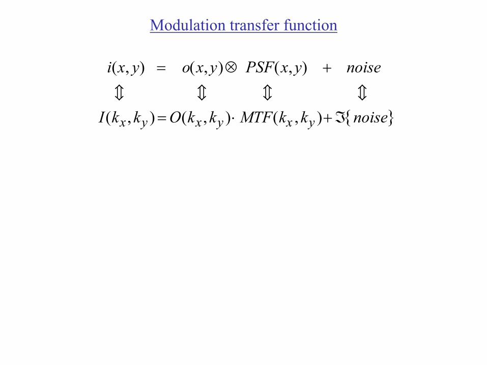
Modulation transfer function

i(x, y) = o( x, y) ⊗ PSF( x, y) + noise c c c c

I (kx , ky ) = O(kx , ky ) ⋅ MTF(kx , ky )+ ℑ{noise}