John Reynolds

FourierTransforms

Joseph Fourier1768-1830

Outline

• Basic properties of the Fourier transform• Discrete form and the FFT • Simple example applications

• Applications in radio astronomy;– Synthesis imaging and the u-v plane – Frequency conversion– The Sampling Theorem– Advanced signal processing (DSP)– filter-banks, spectroscopy

Fourier Integral Transform

dtethfH ift

2)()(

dfefHth ift

2)()(Fourier integral transform

Inverse transform

Mutant forms;

i j (Engineering) 2πf ω (Pure maths or theoretical physics) f,t x,y Individual cosine, sine transforms

Basic Properties I

a . h(t) a . H(f) linearity h(t) + g(t) H(f) + G(f) linearity

h(t) is real H(-f) = H(f)* symmetry

h(t) is imag’ry H(-f) = -H(f)*

h(-t) = h(t) H(-f) = H(f)

h(t) real,even H(f) real,even

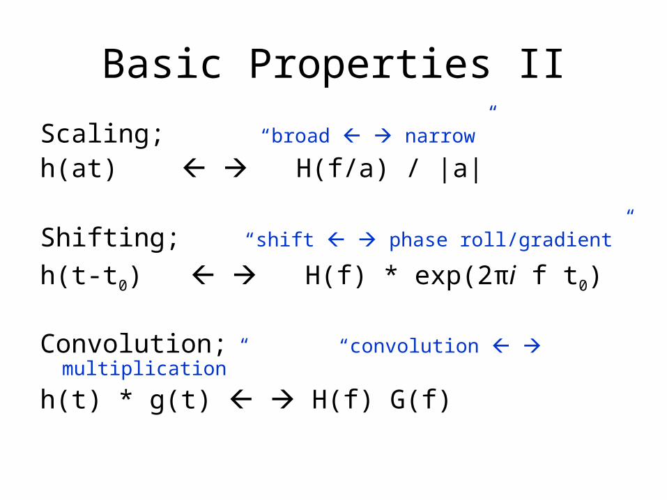
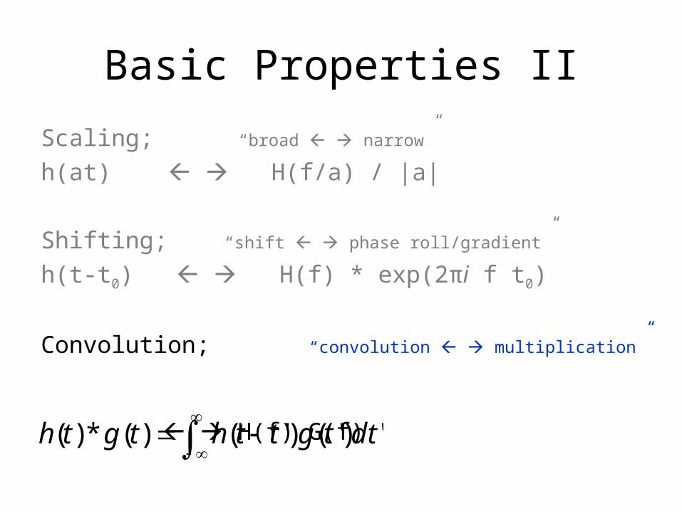
Basic Properties II

Scaling; “broad narrow” h(at) H(f/a) / |a|

Shifting; “shift phase roll/gradient”

h(t-t0) H(f) * exp(2πi f t0)

Convolution; “convolution multiplication”

h(t) * g(t) H(f) G(f)

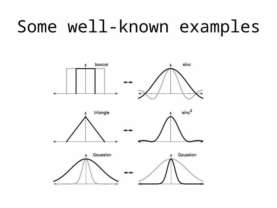
Some well-known examples

The Dirac delta

The humble sinusoid

)()cos( 21 titi eet

Dirac comb or “shah” Ш

dt df=1/dt

Scaling; “broad narrow”

h(at) H(f/a) / |a|

Shifting; “shift phase roll/gradient”

h(t-t0) H(f) * exp(2πi f t0)

Convolution; “convolution multiplication”

H(f) G(f)

Basic Properties II

')'()'()(*)( dttgtthtgth

Convolution – a simple example

*

=

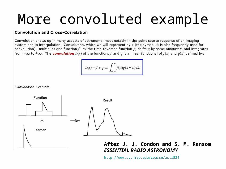
More convoluted example

After J. J. Condon and S. M. RansomESSENTIAL RADIO ASTRONOMYhttp://www.cv.nrao.edu/course/astr534

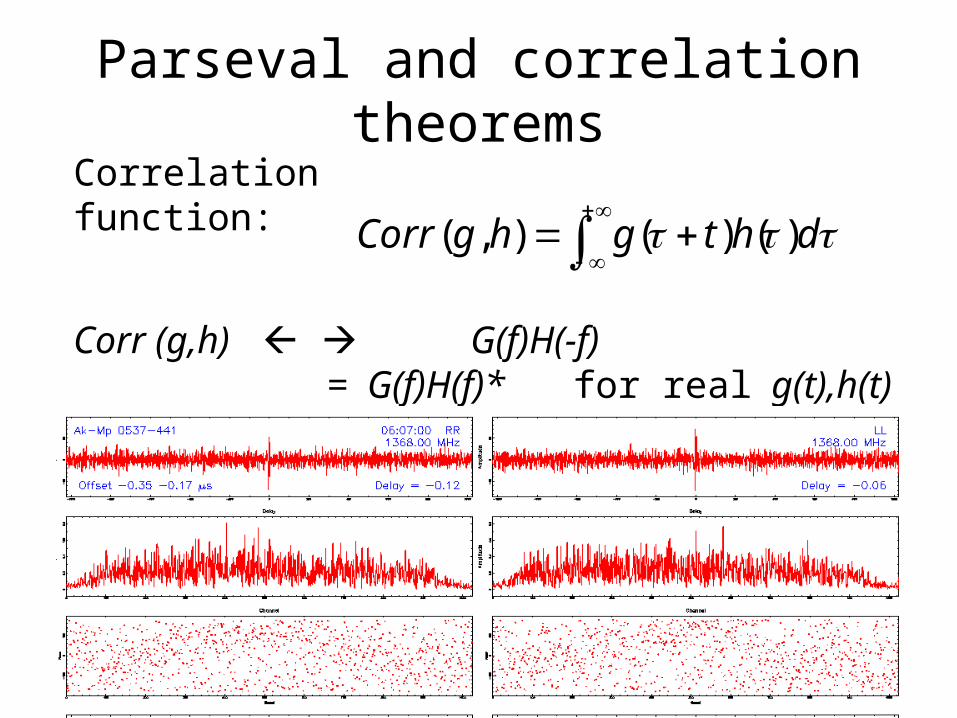
Parseval and correlation theorems

dhtghgCorr )()(),(

Corr (g,h) G(f)H(-f) = G(f)H(f)* for real g(t),h(t)

Corr (g,g) |G(f) |2 (Wiener-Khinchin)

Correlation function:

dffHdtth22

)()(

(Parseval)

Parseval

dffHdtth22

)()(

Energy is conserved!

|H(f)|2 := power spectral density PSD

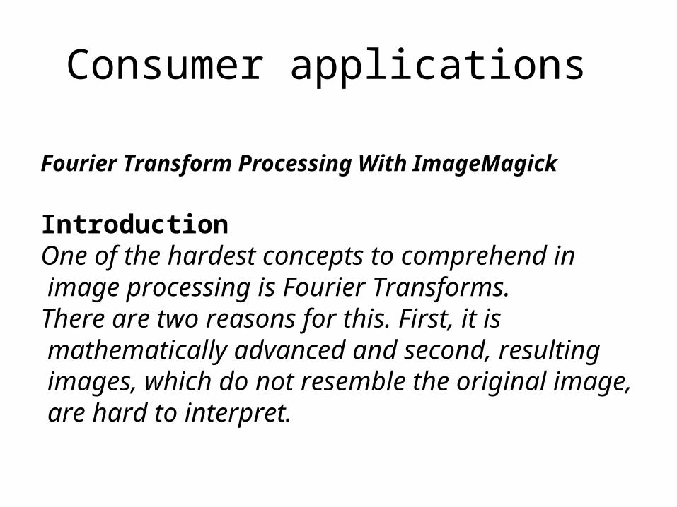
Consumer applications

Fourier Transform Processing With ImageMagick

IntroductionOne of the hardest concepts to comprehend in image processing is Fourier Transforms.There are two reasons for this. First, it is mathematically advanced and second, resulting images, which do not resemble the original image, are hard to interpret.

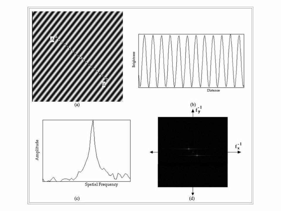
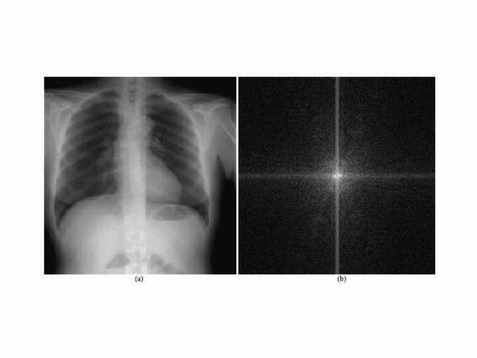
2-D and beyond

dmemlhdlevuH imviul 22 ),(),(

dmdlemlh vmuli .),( )(2

“Top Hat” Airy disk

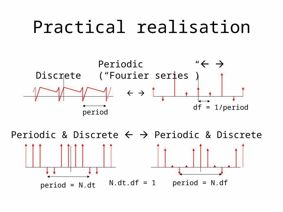
Practical realisation

Periodic Discrete (“Fourier series”)

perioddf = 1/period

Periodic & Discrete Periodic & Discrete

period = N.dt period = N.dfN.dt.df = 1

DFT: Discrete Fourier Transform

Periodic, discretely sampled functions with; t = k.dt, f = n.df, (where N.dt.df = 1)

Replace indefinite integral with summation over N values;

NiknN

k kn ehH /21

0

NiknN

n nNk eHh /21

01

21

01

21

0

N

n nN

N

k k Hh Discrete form of Parseval

All aforementioned properties of Fourier integrals carry over, e.g.;

* One or other of h(t), H(f) function is generally “band-limited”

FFT – the Fast Fourier Transform

Simple DFT requires ~N2 multiplicationsGets very slow with large N

Decompose the NxN matrix intoa product of N sparse matrices

Have reduced to 2 DFTs of order N/2Keep going until you get to order 1.Number of mults now ~N.logN

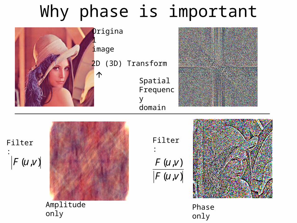
Why phase is important

),( vuF

Originalimage

2D (3D) Transform

),(

),(

vuF

vuF

Amplitude only

Phase only

Filter:

Filter:

SpatialFrequencydomain

error

correction

by spatial

masking

Applications in radio astronomy

• Aperture synthesis imaging

• Frequency conversion

• Sampling theorem

• Signal processing (spectrometers, PFBs)

u-v plane

East

Synthesis interferometer: we cross-correlate each pair of antennas

2-1 1-2 2-3 1-33-1 3-2321

Distribution function A(x,y) in antennas Transfer function W(u,v)

For n antennas n(n-1)/2 baselines (points) in u-v plane

u

1-1, 2-2 etc excluded!

aperture plane u-v plane

spatialauto-correlation

ASKAP – Australian SKA Pathfinder

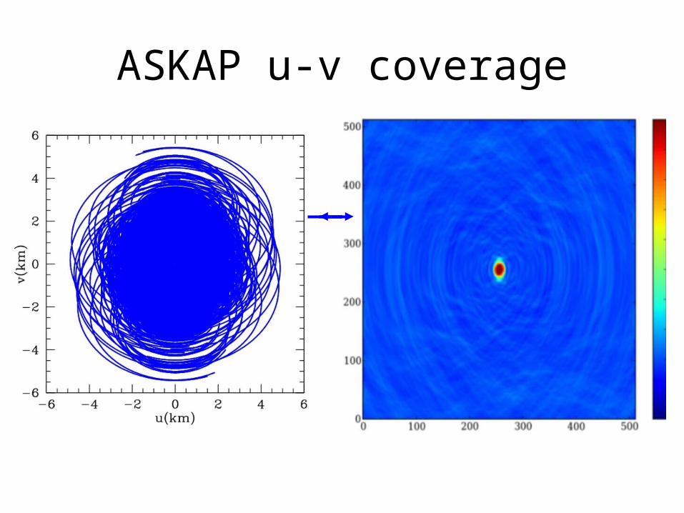
ASKAP u-v coverage

Fourier transform of sky brightness is a function in the u-v plane

λ/a

Complex visibility

dmdlemlBmlAvuV mvuli .),(),(),( )(2

B(l,m) := sky brightness in direction l,m

A(l,m) := antenna reception pattern

Mixing it down – Frequency Conversion

Signal 1

Signal 2

Signal 1 × Signal 2

Mixer (Multiplier)

Frequency Frequency

cos(ω1t)cos(ω2t)=½[cos((ω1+ω2)t)+ cos((ω1-ω2)t)]

Δf Δf

1*2

Difference Sum

cos(ωt) = ½[exp(iwt)/2 + exp(-iwt)]

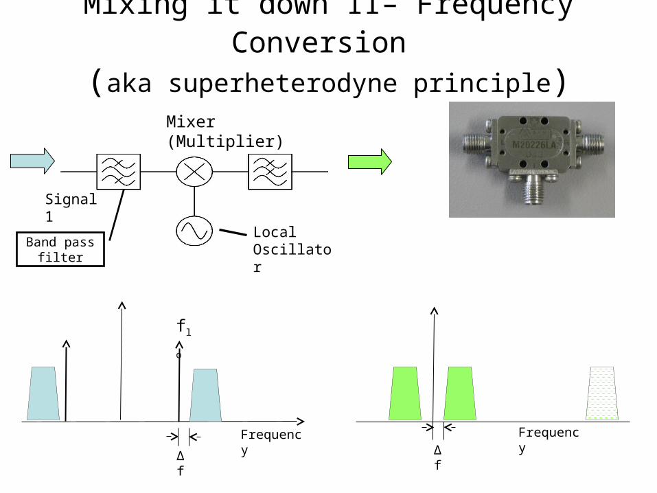
Mixing it down II– Frequency Conversion (aka superheterodyne principle)

Signal 1

Mixer (Multiplier)

Frequency Frequency

Δf Δf

Local Oscillator

flo

Band pass filter

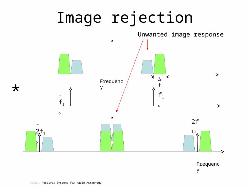
Image rejection

CSIRO. Receiver Systems for Radio Astronomy

Frequency

Frequency

Δf

flo* -flo

2flo-2flo

Unwanted image response

Negative frequencies: learn to love them!

titi eet 21)cos(

ω-ω

Analytic signal of real f(t);

h(t) h(t) + i.H(f)(t)

H(f) := Hilbert transform

cos(ωt) cos(ωt) + i.sin(ωt)

Single Sideband Mixers

CSIRO. Receiver Systems for Radio Astronomy

Signal

2√2cos(ω1t) √2cos[(ωLO- ω1)t] (USB) 0 (LSB)

SignalLocal Oscillator

Lower sideband

Upper sideband

Sampling Theorem – History

The theorem is commonly called the Nyquist sampling theorem; since it was also discovered independently by E. T. Whittaker, by Vladimir Kotelnikov, and by others, it is also known as Nyquist Shannon–Kotelnikov, Whittaker–Shannon–Kotelnikov, Whittaker–Nyquist–Kotelnikov–Shannon, WKS, etc., sampling theorem, as well as the Cardinal Theorem of Interpolation Theory.

It is often referred to simply as the sampling theorem.

(From Wikipedia)

Sampling Theorem (Shannon)

If a function x(t) contains no frequencies higher than B hertz, it is completely determined by giving its ordinates at a series of points spaced 1/(2B) seconds apart.

tsamp < 1 / 2B

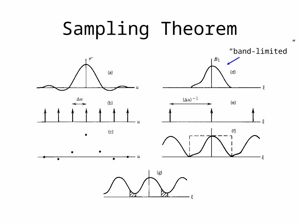
Sampling Theorem“band-limited”

ts=1/B (x2 undersampled)ts=1/2B (Nyquist) “aliased response”, or “aliasing”

Sampling Theorem continued

Also;

Radiotelescopes – Christiansen and Högbom

Radio Astronomy – J.D. Kraus

Principles of Interferometry and Synthesis in Radio Astronomy - Thompson, Moran, Swenson

Aliased sampling

Frequency

fs = 1/tsamp

*

2fs

B

Sampling theorem: fs = 1/tsamp > 2B

3fs -fs -2fs

Baseband 3rd Nyquistzone

Recent Trends

• Faster, cheaper, samplers

• Faster, cheaper processing, data storage

Wider sampled bandwidthsFewer downconversion stages

“direct conversion” (no downconversion)

e.g. DRAO receiver at Parkes)

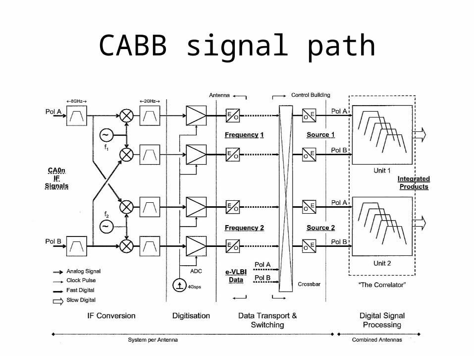
CABB signal path

This talk ends here!