Recession flow analysis of the Blue Nile River

HYDROLOGICAL PROCESSESHydrol. Process. 17, 2825–2835 (2003)Published online in Wiley InterScience (www.interscience.wiley.com). DOI: 10.1002/hyp.1436

Recession flow analysis of the Blue Nile River

Anil Mishra,1* Takeshi Hata,1 A. W. Abdelhadi,2 Akio Tada3 and Haruya Tanakamaru1

1 Department of Regional Environment, Graduate School of Science and Technology, Kobe University, Kobe, Japan2 Agricultural Research Corporation, PO Box 126, Wad Medani, Sudan

3 Faculty of Agriculture, Kobe University, Kobe, Japan

Abstract:

Estimates of the amount of recession flow can be derived from streamflow records. Such estimates are critical inthe assessment of low flow characteristics for the Blue Nile River, from which about two-thirds of the irrigationrequirements in Sudan are satisfied. The recession flow hydrograph can be estimated by fitting the conceptual non-linear storage outflow model using an iterative algorithm. An analytical model to forecast the Blue Nile recession flowis developed and the performance of the model is compared to the previous Blue Nile recession flow model. In theproposed model, a simple linear regression equation is introduced to illustrate the effect of antecedent flow on therecession parameter. Results indicate that the model can provide a simple and reliable method to predict the recessionflow of the Blue Nile River. Copyright 2003 John Wiley & Sons, Ltd.

KEY WORDS recession forecast; storage–discharge relationship; analytical model; Blue Nile River

INTRODUCTION

The Blue Nile River originates at Lake Tana in the Ethiopian Highlands. The river contributes nearly 80% ofthe water that enters the Nile River during high-flow season, with the remainder being supplied by the WhiteNile and other tributaries. The Blue Nile provides a vital source of freshwater to the downstream riparianusers, Sudan and Egypt. The Blue Nile within Ethiopia has a very limited rain gauge coverage and limitedmeteorological data. In the absence of sufficient hydrological and meteorological data from the upper stream,the hydrological assessment of the Blue Nile River becomes more dependent on downstream measurements.Most studies of the Blue Nile typically begin near the Sudan–Ethiopia border and progress towards Khartoum.The Blue Nile catchment area is about 175 000 km2. A map of the Blue Nile catchment is shown in Figure 1.The Blue Nile flow is characterized by severe seasonality and the bulk of runoff (70% on average) occursbetween July and September. Since the dry season flows of the Blue Nile and its tributaries represent only30% of the annual flow, the water stored from the previous season in the two reservoirs is essential forirrigation and for hydropower generation. Thus the aim of the Sudanese authorities is to maximize irrigation,hydropower and water supply while minimizing sedimentation within the framework of the 1959 River Nilewater agreement between Egypt and Sudan. Several attempts have been made to forecast the Blue Nile lowflow for this purpose. To estimate the recession flow of the Blue Nile River, this study uses a non-linearreservoir algorithm, in which the effect of antecedent flow on the recession parameter is included.

RECESSION FLOW ANALYSIS AND STORAGE–DISCHARGE RELATIONSHIP

The recession flow in a natural river system can be defined as the flow resulting from the drainage fromthe groundwater storage or other delayed sources (Hall, 1968). During the dry season, water is gradually

* Correspondence to: Anil Mishra, Department of Regional Environment, Graduate School of Science and Technology, Kobe University,Kobe 657-8501, Nada-ku, Japan. E-mail: [email protected]

Received 30 June 2002Copyright 2003 John Wiley & Sons, Ltd. Accepted 10 October 2002

2826 A. MISHRA ET AL

Longitude (° E)

North Africa

Study area

Latit

ude

(° N

)

Figure 1. Map of the Blue Nile River catchment with the outlet at El Deim, Sudan

removed from the catchment through evapotranspiration and ground water discharge into a stream. A depletionof streamflow discharge during these periods is known as a recession, and is reflected in a streamflowhydrograph by a recession curve (Tallaksen, 1995). The streamflow recession curve effectively representsthe storage–outflow relationship for the river catchment (Smakhtin, 2001). The recession of a streamflowhydrograph reflects the total effect of the various physical watershed factors affecting runoff (Singh and Stall,

Copyright 2003 John Wiley & Sons, Ltd. Hydrol. Process. 17, 2825–2835 (2003)

RECESSION FLOW ANALYSIS 2827

1971). Comprehensive reviews by Hall (1968), Tallaksen (1995) and Smakhtin (2001) reveal that most studieshave theoretically or empirically dealt with the component of hydrograph recession, which characterizes thestorage–discharge relationship.

Modelling recession as a linear reservoir outflow

Boussinesq (1877) developed the basic non-linear differential equation governing flow in aquifers. Heproposed an approximate linear solution, which can be expressed in a simple exponential equation,

Qt D Q0 exp(

� t

k

)�1�

where Qt is discharge at time t, Q0 is the initial discharge and k is the recession constant. The exponentialfunction implies that the aquifer behaves like a single linear reservoir where storage S is proportional to outflowQ, thus S D kQ. The most common measure of recession is the recession constant k. Many investigators(Barnes, 1939; Singh and Stall, 1971; Nathan and McMahon, 1990 and others) have proposed methods toderive the recession constant using different estimation procedures.

Non-linear representation

As the simple exponential equation generally does not satisfactorily represent the recession flow over a widerange of flows, the catchment storage should be given a non-linear representation or conceptually modelledby more than a single reservoir (Tallaksen, 1995). Brutsaert and Nieber (1977) and Szilagyi et al. (1998)suggested that recession flow could be modelled with the non-linear Dupuit–Boussinesq model. Kimura(1956) proposed a non-linear storage outflow function as part of his work on runoff estimation. Theoreticaland numerical analyses of streamflow recession (Werner and Sundquist, 1951; Prasad, 1967; Fukushima,1988; Wittenberg, 1999; Wittenberg and Sivapalan, 1999) have shown that the storage–discharge relationshipis non-linear. Ando et al. (1983), during their experimental analysis, also obtained a similar result from theequipped natural basin located near Tokyo, Japan.

Multiple linear reservoirs

Instead of applying a non-linear reservoir equation, the recession curve can be modelled as a combinationof linear reservoirs (Tallaksen, 1995). Griffiths and Clausen (1997) suggested the approach whereby recessionflow is modelled as the result of depletion in a multistorage catchment. Clausen (1992) and Moore (1997)suggested a two-linear-reservoir recession model. The physical basis of the parallel linear reservoir model,however, only appears evident in a few special cases (Clausen, 1992; Radczuk and Szarska, 1989) andin most catchments it is unlikely that the unconfined aquifer is divided into independent storage zones(Wittenberg, 1999). The identification of the actual non-linearity of runoff processes is a step towardsphysically based modeling (Wittenberg and Sivapalan, 1999). Variations in hydrologic, meteorologic andgeometric characteristics of the river basins render the linear reservoir approach unsuitable for large catchments(Hamad, 1993). The present study aims to develop a recession forecast model for the Blue Nile River. Tomodel the Blue Nile recession flow, this study uses a non-linear storage–outflow algorithm, with the parametersderived from the observed streamflow data, and additionally, the recession parameter is related to the steepnessof the recession derived from the preceding flood.

DATA SELECTION

The Blue Nile is characterized by severe seasonality and the bulk of runoff (70% on average) occurs betweenJuly and September. From October to March, the irrigation of July-sown cotton and winter wheat, in additionto hydroelectric power production, are dependent on stored water from dams (El-Awad, 2000). Since the



combined capacity of the two reservoirs falls short of the total requirements, the shortage has to be accountedfor by using the natural river flow during the recession time. Flow in the Blue Nile increases again inMarch–May due to equatorial spring rains on the southern tributaries (Sutcliffe and Parks, 1999). Therecession forecast is required immediately after the flood has tailed off. During this period an irrigationwater crisis occurs, particularly during the reproductive stage of cotton, as both agriculture and hydroelectricpower compete for water (El-Awad, 2000). The decision regarding the winter plantation has to be taken asearly as the first week of October (Abdelhadi et al., 2000). The mean ‘10-days’ discharge data set used in thisstudy is observed data from Roseires/El Deim station, Sudan. Using the mean ‘10-days’ discharge of the BlueNile, each year has 36 ‘10-day’ periods, three for each month. The recession candidates for calibration areselected based on the following criteria: (a) the recession period for each year involves at least 15 ‘10-day’discharges from October to February; (b) years with regular recession flows are chosen as recession candidatesand years with intermittent wet periods are excluded; (c) the discharge decreases during the recession period.Based on these criteria, ‘10-day’ discharges from October to February, taken from the selected 28 annual dataperiods (1917–1970), are used as a set of recession candidates for calibration. Similarly, a 22-year validationperiod, which also excludes years with the abnormal recession periods, is selected from the total data period(1971–1997).

RECESSION FLOW FORECAST MODEL FOR THE BLUE NILE RIVER

In the present study the recession curve equation is used in the following expression as in Wittenberg (1999)to determine discharge after time t at an initial discharge Q0,

Qt D Q0

[1 C �1 � b�Q1�b

0

abt

]1/�b�1�

�2�

The equation is obtained after combining the non-linear storage–discharge relationship, S D aQb and thecontinuity equation of a reservoir without inflow, dS/dt D �Q. For S in m3 and Q in m3 s�1 the coefficienta has the dimension m3�3b sb. The exponent b is dimensionless. Brutsaert and Nieber (1977) derived andused a similar equation in accordance with the non-linear Dupuit–Boussinesq model. In this study, Q0 istaken as the mean ‘10-days’ discharge of the first period of October and Qt is the discharge after timeperiod t. The parameter values of a and b are calibrated by an iterative least-squares fitting method from theselected recession candidates. By systematically varying the parameter b, the value of parameter a is solvedat each iteration step. The set of a and b values providing the best fit to the observed curve is consideredas representing the properties of the aquifer. The mean value of exponent parameter b D 0Ð6 with a standarddeviation of 0Ð12 is thus obtained for the calibration period. For most practical purposes, it seems reasonableto fix the exponent b at the mean or dominant value, and to allow the coefficient a to vary. The variation ofa can be determined from the observed flow recessions (Wittenberg, 1999),

S D a1Q0Ð6 �3�

a1 (the value of a for b D 0Ð6) is then determined from the second calibration. Wittenberg and Sivapalan(1999) found that the determined coefficient a1 has a significant variation. They related the variation of a1 tothe seasonal variation of evapotranspiration. Since the recession forecast of the Blue Nile has to be performedshortly after the wet season, when the interflow and bank storage may be contributing considerably to theriver flow (Hamad, 1993), the effect of antecedent flow should also be taken into consideration. The variationof the determined coefficient a1 is related to the steepness of the recession derived from the magnitude ofthe preceding flood in this study. Rainfall in the Blue Nile Basin is highly seasonal which creates a highlyseasonal flood regime for the Blue Nile River, and this reflects a long flow recession. The recession hydrographreflects the rate at which water is drained from the catchment. At the start of the recession, when quick storm



0

2000

4000

6000

8000

10000

12000

14000

16000

Apr

il

Feb

.

Jan.

Sep

t.

Aug

.

July

June

May

Flo

w (

m3

× 10

6 )

Mar

.

Dec

.

Nov

.

Oct

.

Figure 2. Long-term mean monthly flows of the Blue Nile River at El Deim (1913/14–1997/98)

response dominates the streamflow generating mechanisms (Verma and Brutsaert, 1971), recession behaviourcan be explained by considering the magnitude of the preceding flood. Szilagyi and Parlange (1998) similarlycharacterized recession behaviour in accordance with the non-linear Dupuit–Boussinesq model. Long-termmean monthly flow (1913/14–1997/98) of the Blue Nile is shown in Figure 2, which illustrates a peak inAugust, after which the Blue Nile flow starts to fall. The period of flow from August to October is clearlythe time when quick storm response dominates the streamflow generating mechanisms. Thus in this study therecession behaviour of every year is expressed in terms of the discharge ratio (CurASO1/meanASO1), whereASO1 D AD C SD C O1 and AD D ‘10-days’ discharge of August (three periods), SD D ‘10-days’ dischargeof September (three periods), O1 D ‘10-days’ discharge of October 1st period, CurASO1 D current year’sASO1 discharge, meanASO1 D mean discharge of ASO1 period from the calibration years. (The mean ‘10-days’ discharge data were used for this study, which means that each month has three ‘10-day’ periods asexplained in the data selection section.)

Simple regression analysis (Figure 3) is performed to relate the recession behaviour of the calibration periodto the obtained a1 value when b D 0Ð6, and the following relation is then obtained, with R2 D 0Ð689

a1 D 19Ð201 C 20Ð474(

CurASO1

meanASO1

)�4�

The recession flow for the Blue Nile from October to February was then determined. Thus the modelprovides a simple method for forecasting recession flow.

PREVIOUS BLUE NILE RECESSION FLOW MODEL

Abdelhadi et al. (2000) developed an analytical model for forecasting the Blue Nile recession flow based onthe non-linear reservoir model, similar to Equation (2). For parameter calibration they used a slope coefficientm, where m D n/a�1 � n� and n D 1 � b. The sequences of similar years according to flood magnitude weregrouped into three different categories: dry, wet and normal years. The value of n for each group of similaryears was determined and the common value was obtained as 0Ð4 (i.e., b D 0Ð6), and m was determined bymultivariate regression analysis (R2 D 0Ð645�

m D 0Ð02 C 0Ð0027 log(

curASO1

preASO1

)� 0Ð021 log

(AgSp

JAS

)� 0Ð005 log (Pannual) �5�



0.7 0.8 0.9 1.0 1.1 1.2 1.3 1.40

10

20

30

40

50

60

70

80

a =19.201 + 20.474(CurASO1/mean ASO1)R2 = 0.689

a va

lue

ASO1 ratio

Figure 3. Parameter a versus ASO1 ratio for the calibration period

where Pannual is the ratio of the previous annual flow to the mean flow of the calibration period. The ratioof the mean flow during August, September and the first period of October of the current year to that of thesame period of the previous year was computed and named curASO1/preASO1. And the ratio of the currentyear’s mean flow during August and September to the mean flow of July, August and September during thecalibration period was computed and named AgSp/ JAS.

The two regression equations, Equation (4) and Equation (5), are compared. Figure 3 describes the simpleregression Equation (4), while the multivariate regression Equation (5) is summarized in Table I. The R2

measure of the goodness of fit clearly advocates the effectiveness of the proposed model. For the proposedmodel in Equation (3), with one predictor variable ASO1 ratio, R2 is 0Ð689, a clear increase over the model inEquation (5), which uses three predictor variables. Moreover, the three independent variables in Equation (5)did not show strong correlation. Table I clearly demonstrates through t-test analysis that Equation (5) is only asimple (bivariate) regression. As two model parameters are not significantly different from zero, the equationis flawed due to the inclusion of insignificant predictor variables. Also, in the previous model, in analysing therecession parameter, years with the intermittent flow (non-recession flow) from the calibration period werenot excluded, which also makes their analysis questionable. Thus, analyses show that Equation (4) providesa simple and reliable method to predict the recession flow of the Blue Nile.

RESULTS AND DISCUSSION

The recession flows of the Blue Nile for the period of 50 years, which includes both calibration and validationperiods, were estimated and the results compared to the previous Blue Nile recession forecast model ofAbdelhadi et al. (2000). Four indices of efficiency criteria were used in the study to evaluate the performanceof the model. Table II gives a description of these efficiency criteria. The most popular measure is the RMSEcriterion, which evaluates the sum of the squares of the flow residuals. RMSLE evaluates the sum of the squaresof the residuals of the logarithms of the flows. To estimate the efficiency of the fit, the NSE (Nash–Sutcliffeefficiency) criterion is used. The value of NSE is always expected to approach unity for a perfect simulationof the observed flow series. Criterion MAE (mean absolute error) gives an indication of the average absolutedeparture of a model from the observed discharge. This criterion may be preferred for forecasting, when



Table I. Summary of multivariate regression analysis Equation (5)

Regression coefficients Coefficient Łt

Constant 0Ð02 22Ð030Predictor variable 1 0Ð0027 0Ð375Predictor variable 2 �0Ð021 �2Ð402Predictor variable 3 �0Ð005 �0Ð481Model summary R2 ŁŁAdjusted R2

0Ð645 0Ð621

Ł The values are the t-ratios of the estimated model parameters.ŁŁ The values of R2 are adjusted for the number of degrees of freedom whichremain after parameter estimation.

Table II. Efficiency criteria, description and formula

Criterion Description Formula

RMSE Root mean squared residuals

√√√√ 1N

N∑iD1

(Qo,i � Qe,i

)2

RMSLE Root mean squared log residuals

√√√√ 1N

N∑iD1

(log Qo,i � log Qe,i

)2

NSE The Nash and Sutcliffe efficiency criterion 1Ð0 �

N∑iD1

(Qo,i � Qe,i

)2

N∑iD1

(Qo,i � Qo

)2

MAE Mean absolute error 1N

N∑iD1

jQo,i � Qe,ij

Qo, Qe, Qo are observed flow, estimated flow and the mean observed flow

Table III. Comparison of model performance based on four indices of efficiency criteria

No. ofyears

RMSE criterion(mean value)

RMSLE criterion(mean value)

NSE criterion(mean value)

MAE criterion(mean value)

Model Previousmodel

Model Previousmodel

Model Previousmodel

Model Previousmodel

Calibration 28 years 8Ð174 9Ð140 0Ð043 0Ð049 0Ð975 0Ð964 5Ð101 5Ð625Validation 22 years 8Ð940 9Ð581 0Ð065 0Ð075 0Ð961 0Ð926 5Ð944 6Ð628

it is important to be as close as possible to the observed flow at every time step (Ye et al., 1997). Thevalues of RMSE, RMSLE and MAE criteria are expected to be at a minimum for better simulations. Table IIIpresents the RMSE, RMSLE, NSE and MAE statistics for the mean 28 years of the calibration and for themean 22 years of the validation period. Clearly the proposed method is effective for improving prediction



0

20

40

60

80

100

120

140

160

Oct

II

Oct

III

Nov

I

Nov

II

Nov

III

Dec

I

Dec

II

Dec

III

Jan

I

Jan

II

Jan

III

Feb

I

Feb

II

Feb

III

model

previous model

0

20

40

60

80

100

120

140

160

180

Oct

II

Oct

III

Nov

I

Nov

II

Nov

III

Dec

I

Dec

II

Dec

III

Jan

I

Jan

II

Jan

III

Feb

I

Feb

II

Feb

III

model

observed flow

previous model

Year 1919/20(a)

Year 1953/54(b)

Flo

w (

m3

× 10

6 d−1

)F

low

(m

3 ×

106 d

−1)

observed flow

10 days flow

10 days flow

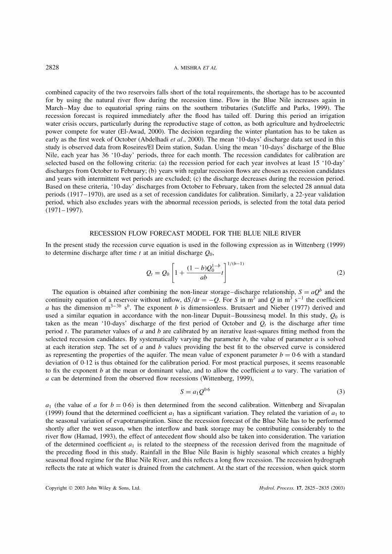
Figure 4. Theoretical recessions and observed flows for the two different years from the calibration period

accuracy. The developed model appears to provide a substantially better fit than the previous model, whichindicates that despite the simplification, the method seems promising in predicting recession flow of theBlue Nile River. For further analysis of the models’ prediction performance, Figures 4a,b and 5a,b presenta comparison of theoretical recessions of the two different models to the observed flows. The four differentyears shown in Figures 4a,b and 5a,b represent both calibration and validation periods. Results indicate thatthe method provides a substantially better fit to the observed data than the previous method. The ability topredict the amount of streamflow recession easily and more accurately should prove extremely valuable, sincethe decision on the total dry season plantation area depends merely on the expected recession flow of theBlue Nile River. The magnitude of the preceding flood attributing the rate at which water is drained fromthe catchment can be determined from the steepness of the recession hydrograph. The existence of quickstorm response components on the receding limb of the hydrograph has been widely studied (Brutsaert andNieber, 1977; Verma and Brutsaert, 1971; Chapman and Maxwell, 1996). Recently Szilagyi and Parlange



0

20

40

60

80

100

120

140

160

180

Oct

II

Oct

III

Nov

I

Nov

II

Nov

III

Dec

I

Dec

II

Dec

III

Jan

I

Jan

II

Jan

III

Feb

I

Feb

II

Feb

III

model

observed flow

previous model

0

20

40

60

80

100

120

140

160

Oct

II

Oct

III

Nov

I

Nov

II

Nov

III

Dec

I

Dec

II

Dec

III

Jan

I

Jan

II

Jan

III

Feb

I

Feb

II

Feb

III

model

observed flow

previous model

10 days flow

Year 1980/81(a)

(b)

10 days flow

Year 1991/92

Flo

w (

m3

× 10

6 d−1

)F

low

(m

3 ×

106 d

−1)

Figure 5. Theoretical recessions and observed flows for the two different years from the validation period

(1998) characterized and analysed the receding limb of a hydrograph according to the discharge rate from aflood event and discovered the importance of quick storm response as a guiding factor for recession tendency.In the Blue Nile, the August to October flow is the region where quick storm response components dominatethe streamflow generating mechanisms. The existence of storm response components on the receding limb ofthe hydrograph appears to be a reasonable assumption in this study, since it is also confirmed by the fact thatthe numerically obtained parameter value a1 varies with the recession behaviour derived from the magnitudeof the preceding flood.

CONCLUSION

Peaking in August, the Blue Nile flow starts to fall in September as rain water supply to the river beginsto decrease. From October, the irrigation of cotton and winter wheat, in addition to hydroelectric powergeneration, are dependent on stored water from dams. There are two reservoirs in the Sudanese territory of



the Blue Nile, Roseires and Sennar, with a combined storage capacity of 3 km3. The reservoirs are operated inseries. Operating rules have been developed to minimize sedimentation and to optimize hydropower productionin terms of water availability and irrigation demands (Hamad, 1993). The problem is complex becauseenergy demand increases during the hot season and doesn’t coincide with irrigation releases (Sutcliffe andPark, 1999). The upper reservoir, Roseires (capacity 275 MW), releases all water to the Sennar dam after itproduces hydropower. The Sennar dam was built to store and divert irrigation water for the Sudan–Gezirairrigation scheme (about 800 000 ha). From Sennar dam (capacity 15 MW) less than 15% of the waterpassing downstream is utilized for hydropower generation because the installed capacity is very small.The dry season recession flow of the Blue Nile, which forms a useful supplement to the stored water,can be better forecasted using the non-linear storage–discharge relationship. The parameter a of the non-linear storage–outflow relationship is related to the recession behaviour, which is expressed as the ASO1ratio and derived on the basis of the preceding flood. The obtained relation between parameter a and theASO1 ratio identifies the importance of quick storm response components in the aquifer–stream interaction.The study has shown that the proposed method is effective and relatively simple for improving predictionaccuracy. The study also illustrates that the observed streamflow data hold indispensable information aboutthe foregoing hydrological processes. Further investigation of aquifer parameters, in relation to flow recession,might characterize the model on a more physical and less empirical footing.

ACKNOWLEDGEMENTS

This work is part of a study supported by a Grant-in-Aid (No. 12574015) from the Japan Society for thePromotion of Science. The authors are very grateful to the staff of the Agricultural Research Corporation andMinistry of Irrigation & Water Resources, Sudan for their kind cooperation. The authors are grateful for theconstructive comments provided by two anonymous reviewers, which improved the paper.

REFERENCES

Abdelhadi AW, Hata T, Hamad OE. 2000. A recession-forecast model for the Blue Nile River. Nordic Hydrology 31: 41–56.Ando Y, Musiake K, Takahasi Y. 1983. Modelling of hydrologic processes in a small natural hillslope basin, based on the synthesis of

partial hydrological relationships. Journal of Hydrology 64: 311–337.Barnes BS. 1939. The structure of discharge–recession curves. Transactions of the American Geophysical Union 20: 721–725.Boussinesq J. 1877. Essai sur la theorie des eaux courantes. Memories presentes par divers savants a l’Academie des Sciences de l’Institut

National de France, Tome XXIII, No. 1.Brutsaert W, Nieber JL. 1977. Regionalized drought flow hydrographs from a mature glaciated plateau. Water Resources Research 13:

637–643.Chapman TG, Maxwell AI. 1996. Baseflow separation-comparison of numerical methods with tracer experiments. 23rd Hydrology and Water

Resources Symposium, Hobart, Australia; 539–545.Clausen B. 1992. Modelling streamflow recession in two Danish streams. Nordic Hydrology 23: 73–88.El-Awad S. 2000. Effects of irrigation interval and tillage systems on irrigated cotton and succeeding wheat crop under a heavy clay soil in

the Sudan. Soil and Tillage Research 55: 167–173.Fukushima Y. 1988. A model of river flow forecasting for a small forested mountain catchment. Hydrological Processes 2: 167–185.Griffiths GA, Clausen B. 1997. Streamflow recession in basins with multiple water storages. Journal of Hydrology 190: 60–74.Hall FR. 1968. Base flow recessions—a review. Water Resources Research 4: 973–983.Hamad OE. 1993. Optimal operation of a reservoir system during a dry season. PhD thesis, University of Newcastle upon Tyne, Department

of Civil Engineering; 1–227.Kimura T. 1956. Storage–discharge relationship in a river basin during floods and its application to the runoff estimation—I. Civil

Engineering 5: 1–6 (in Japanese).Moore RD. 1997. Storage–outflow modelling of streamflow recessions, with application to a shallow-soil forested catchment. Journal of

Hydrology 198: 260–270.Nathan RJ, McMahon TA. 1990. Evaluation of automated techniques for base flow and recession analyses. Water Resources Research 26:

1465–1473.Prasad R. 1967. A nonlinear hydrologic system response model. Journal of Hydraulic Division 4: 201–221.Radczuk L, Szarska O. 1989. Use of the flow recession curve for the estimation of conditions of river supply by underground water.

FRIENDS in Hydrology, IAHS Publication 187: 67–74.



Singh KP, Stall JB. 1971. Derivation of base flow recession curves and parameters. Water Resources Research 7: 292–303.Smakhtin VU. 2001. Low flow hydrology: a review. Journal of Hydrology 240: 147–186.Sutcliffe JV, Parks YP. 1999. The Hydrology of the Nile. IAHS Special Publication. 5: 1–179.Szilagyi J, Parlange MB. 1998. Baseflow separation based on analytical solution of the Boussinesq equation. Journal of Hydrology 204:

251–260.Szilagyi J, Parlange MB, Albertson JD. 1998. Recession flow analysis for aquifer parameter determination. Water Resources Research 34:

1851–1857.Tallaksen LM. 1995. A review of baseflow recession analysis. Journal of Hydrology 165: 349–370.Verma RD, Brutsaert W. 1971. Similitude criteria for flow from unconfined aquifers. Journal of Hydraulics Division, American Society of

Civil Engineers 97: 1493–1509.Werner PW, Sundquist KJ. 1951. On the ground water recession curve for large watersheds. IAHS Publication 33: 202–212.Wittenberg H. 1999. Baseflow recession and recharge as nonlinear storage processes. Hydrological Processes 13: 715–726.Wittenberg H, Sivapalan M. 1999. Watershed groundwater balance estimation using streamflow recession analysis and baseflow separation.

Journal of Hydrology 219: 20–33.Ye W, Bates BC, Viney NR, Sivapalan M, Jakeman AJ. 1997. Performance of conceptual rainfall–runoff models in low yielding ephemeral

catchments. Water Resources Research 33: 153–166.


Documents

Recession flow analysis of the Blue Nile River