Realized Detection and Capture Probabilities for Giant - · PDF fileOpen-File Report 2015–1200. ... Realized Detection and Capture Probabilities for Giant Gartersnakes (Thamnophis

U.S. Department of the InteriorU.S. Geological Survey

Open-File Report 2015–1200

Prepared in cooperation with the California Department of Water Resources

Realized Detection and Capture Probabilities for Giant Gartersnakes (Thamnophis gigas) Using Modified Floating Aquatic Funnel Traps

Cover: An adult giant gartersnake (Thamnophis gigas). Photograph by Matt Meshriy, U.S. Geological Survey, April 2011.Inset: Modified aquatic funnel trap used to capture giant gartersnakes. Photograph by Margaret Mantor, California Department of Fish and Wildlife, July 2013. Used with permission.


By Brian J. Halstead, Shannon M. Skalos, Michael L. Casazza, and Glenn D. Wylie

Prepared in cooperation with the California Department of Water Resources

Open-File Report 2015-1200

U.S. Department of the Interior U.S. Geological Survey

U.S. Department of the Interior SALLY JEWELL, Secretary

U.S. Geological Survey Suzette M. Kimball, Acting Director

U.S. Geological Survey, Reston, Virginia: 2015

For more information on the USGS—the Federal source for science about the Earth, its natural and living resources, natural hazards, and the environment—visit http://www.usgs.gov or call 1–888–ASK–USGS (1–888–275–8747)

For an overview of USGS information products, including maps, imagery, and publications, visit http://www.usgs.gov/pubprod

Any use of trade, firm, or product names is for descriptive purposes only and does not imply endorsement by the U.S. Government.

Although this information product, for the most part, is in the public domain, it also may contain copyrighted materials as noted in the text. Permission to reproduce copyrighted items must be secured from the copyright owner.

Suggested citation: Halstead, B.J., Skalos, S.M., Casazza, M.L., and Wylie, G.D., 2015, Realized detection and capture probabilities for the giant gartersnake (Thamnophis gigas) using modified floating aquatic funnel traps: U.S. Geological Survey Open-File Report 2015-1200, 36 p., http://dx.doi.org/10.3133/ofr20151200.

ISSN 2331-1258 (online)

http://www.usgs.gov/

http://www.usgs.gov/pubprod

iii

Contents Executive Summary .................................................................................................................................................... 1 Introduction ................................................................................................................................................................. 2

Goals and Objectives .............................................................................................................................................. 3 Biology of Giant Gartersnakes ................................................................................................................................. 5

Detection Probabilities ................................................................................................................................................. 6 Purpose ................................................................................................................................................................... 6 Methods ................................................................................................................................................................... 7

Field Methods ...................................................................................................................................................... 7 Analytical Methods ............................................................................................................................................... 7

Results .................................................................................................................................................................... 9 Detection Probabilities ......................................................................................................................................... 9 Effectiveness for Inference about the Probability of Occurrence ........................................................................ 12

Discussion ............................................................................................................................................................. 16 Capture Probabilities ................................................................................................................................................. 18

Purpose ................................................................................................................................................................. 18 Methods ................................................................................................................................................................. 18

Field Methods .................................................................................................................................................... 18 Analytical Methods ............................................................................................................................................. 21

Results .................................................................................................................................................................. 23 Capture Probabilities .......................................................................................................................................... 23 Abundance ......................................................................................................................................................... 24 Survival .............................................................................................................................................................. 25

Discussion ............................................................................................................................................................. 28 Summary ................................................................................................................................................................... 30 Acknowledgments ..................................................................................................................................................... 30 References Cited ...................................................................................................................................................... 31 Glossary .................................................................................................................................................................... 34

Figures Figure 1. Locations sampled to quantify detection and capture probabilities of giant gartersnakes (Thamnophis gigas) in the Sacramento Valley, California, 2013 ................................................................................ 4 Figure 2. Model-averaged effects of (A) water temperature, (B) number of traps, (C) Julian date, and (D) quadratic function of Julian date on daily detection probability of giant gartersnakes (Thamnophis gigas) in the Sacramento Valley, California, 2013 .............................................................................................................. 11 Figure 3. Distribution of number of successes for (A) 20, and (B) 40 trials when true probability of success = 0.60 versus 0.48 ...................................................................................................................................... 16 Figure 4. Locations sampled for giant gartersnakes (Thamnophis gigas) at Colusa National Wildlife Refuge, California, 2013 ........................................................................................................................................................ 19 Figure 5. Locations sampled for giant gartersnakes (Thamnophis gigas) at Gilsizer Slough, California, 2013 ....... 20 Figure 6. Daily individual capture probabilities (p) of giant gartersnakes (Thamnophis gigas) at an average transect and nine observed transects in the Sacramento Valley, California, 2013 ..................................... 23

iv

Tables Table 1. Means, standard deviations, and ranges of explanatory variables used in the detection component of the occupancy model from which detection probabilities for giant gartersnakes (Thamnophis gigas) were calculated .......................................................................................................................... 9 Table 2. Posterior probabilities of models for the detection component of occurrence of giant gartersnakes (Thamnophis gigas) in the Sacramento Valley, California, 2013 .............................................................................. 10 Table 3. Measures of performance of static occupancy models for estimating differences in probability of occurrence when true probability of occurrence = 0.60 versus 0.48 under different sampling scenarios for giant gartersnakes (Thamnophis gigas) in the Sacramento Valley, California .................................................................. 12 Table 4. Ability of occupancy models to detect a difference in probability of occurrence when true probability of occurrence = 0.60 versus 0.48 under different sampling scenarios for giant gartersnakes (Thamnophis gigas) in the Sacramento Valley, California ........................................................................................ 14 Table 5. Measures of performance of static occupancy models for finite population inference (number of occupied sampled sites) of giant gartersnakes (Thamnophis gigas) in the Sacramento Valley, California .............. 15 Table 6. Measures of performance of closed population models for estimating abundance (N) under different sampling scenarios for giant gartersnakes (Thamnophis gigas) in the Sacramento Valley, California ..................... 24 Table 7. Measures of performance of Cormack-Jolly-Seber models for estimating survival under different sampling scenarios for giant gartersnakes (Thamnophis gigas) in the Sacramento Valley, California ..................... 26 Table 8. Odds ratios for correctly identifying the population with greater survival rates under the specified sampling conditions when the true difference in survival rates between populations is 0.20 .................................... 28

Conversion Factors

International System of Units to Inch/Pound

Multiply By To obtain

Length

millimeter (mm) 0.0393701 inch

meter (m) 3.28084 foot

kilometer (km) 0.621371 mile

Mass

gram (g) 0.00220462 pound

1


By Brian J. Halstead, Shannon M. Skalos, Michael L. Casazza, and Glenn D. Wylie

Executive Summary Rigorous analysis and management of animal populations requires that observers account for

limitations inherent to the detection of those populations and the individuals within them. Researchers are usually unable to see every individual of a population or to even detect some entire populations. Ignoring this imperfect detectability can bias estimates of population characteristics, such as probability of occurrence, abundance, survival, recruitment, and population growth rate. Furthermore, the precision with which these population characteristics are estimated is dependent on detection probabilities (the probability that at least one individual of a species is detected during a survey, given that the species occurs where the survey is conducted) and capture probabilities (the probability that a given individual is observed or captured during a single survey); greater detection and capture probabilities result in less uncertainty about the values of population characteristics and a greater ability to evaluate the effects of variables or experimental treatments on the population characteristic(s) of interest.

Detection and capture probabilities for giant gartersnakes (Thamnophis gigas) are very low, and successfully evaluating the effects of variables or experimental treatments on giant gartersnake populations will require greater detection and capture probabilities than those that had been achieved with standard trap designs. Previous research identified important trap modifications that can increase the probability of snakes entering traps and help prevent the escape of captured snakes. The purpose of this study was to quantify detection and capture probabilities obtained using the most successful modification to commercially available traps to date (2015), and examine the ability of realized detection and capture probabilities to achieve benchmark levels of precision in occupancy and capture-mark-recapture studies.

Occupancy surveys for giant gartersnakes with modified traps resulted in average daily detection probabilities of 0.46 (95-percent credible interval = 0.22–0.76), which was much higher than previous estimates (0.13 [0.09–0.18]). Simulations demonstrated that sampling a site with 50 traps for 28 days or 100 traps for 14 days could reliably distinguish occupied from unoccupied sites. Furthermore, the simulations suggested that the best way to decrease uncertainty in estimates of giant gartersnake occupancy was to increase the number of sampled sites.

2

Capture-mark-recapture surveys of giant gartersnakes at nine locations resulted in mean daily capture probabilities of 0.03 (0.01–0.08). Simulations of populations differing in abundance by 20 individuals demonstrated that sampling for a longer period of time (90 d instead of 60 d) generally resulted in more precise estimates of the number of giant gartersnakes in the sampled area and a greater ability to determine which of the two sites had more snakes. This result must be tempered because of the assumption of population closure (no individuals are born, die, leave, or enter the population during the sampling period [in this case, 60 or 90 d of sampling within a year]). Daily capture probabilities were calculated using individual trap transects of 25 or 50 traps each; increasing the number of traps and the extent of the sampled area would likely increase precision by directly increasing capture probabilities and decreasing movement into and out of the sampled area.

Outcomes of population simulations differing by 0.20 in annual survival contrasted somewhat with outcomes of population simulations differing in the number of snakes. In this case, the most important variable affecting the precision of survival estimates was the duration of the study. Studies that lasted 5 years resulted in much more precise survival estimates than studies that lasted 3 years. Changing the duration of sampling within a year had relatively little effect on the precision of survival estimates. Similar to estimates of the number of snakes, estimates of survival would likely improve with increases in the number of traps and the extent of the sampled area relative to the individual trap transects used to estimate capture probabilities for the simulation study.

Overall, the detection and capture probabilities achieved with modified floating aquatic funnel traps were adequate to detect meaningful differences in the number of occupied sites, abundance, and survival of giant gartersnakes. For occupancy studies, increasing the number of sampled sites is the best means to increase precision in estimates of the probability of occurrence. For abundance and survival estimation, increasing the number of traps and extent of the sampled area will likely increase precision without violating model assumptions. In studies of survival, increasing the duration of the study (that is, number of years of sampling) will greatly improve precision of survival estimates. With 14 days of sampling with 100 traps per site for occupancy, 90 days of sampling per site for abundance, and 5 years of 60 days per year of sampling for survival, using modified floating aquatic funnel traps should result in the ability to detect small differences in the number of sites occupied, differences in abundance between populations that differ in the tens to hundreds of individuals, and differences of 0.2 or greater in survival probabilities of giant gartersnakes.

Introduction The California Department of Water Resources (DWR) manages the State’s water resources in

collaboration with other parties. In fulfilling this role, DWR supports efforts that promote water supply reliability. Water supply reliability can be a difficult goal to achieve, given the large population in California (particularly in arid regions of the State), the extent and importance of agriculture to the California economy, and the dry Mediterranean and desert climates of much of the State. The high demand of water for urban, residential, industrial, and agricultural uses can deplete water resources necessary for plants and wildlife, particularly aquatic and wetland-dependent species. Giant gartersnakes (Thamnophis gigas) comprise an obligate wetland species precinctive to marshes and marsh-like habitats in the Central Valley of California. Because of the loss of nearly all of its native tule (Schoenoplectus spp.) marsh habitat, giant gartersnakes are listed under the U.S. and California Endangered Species Acts

3

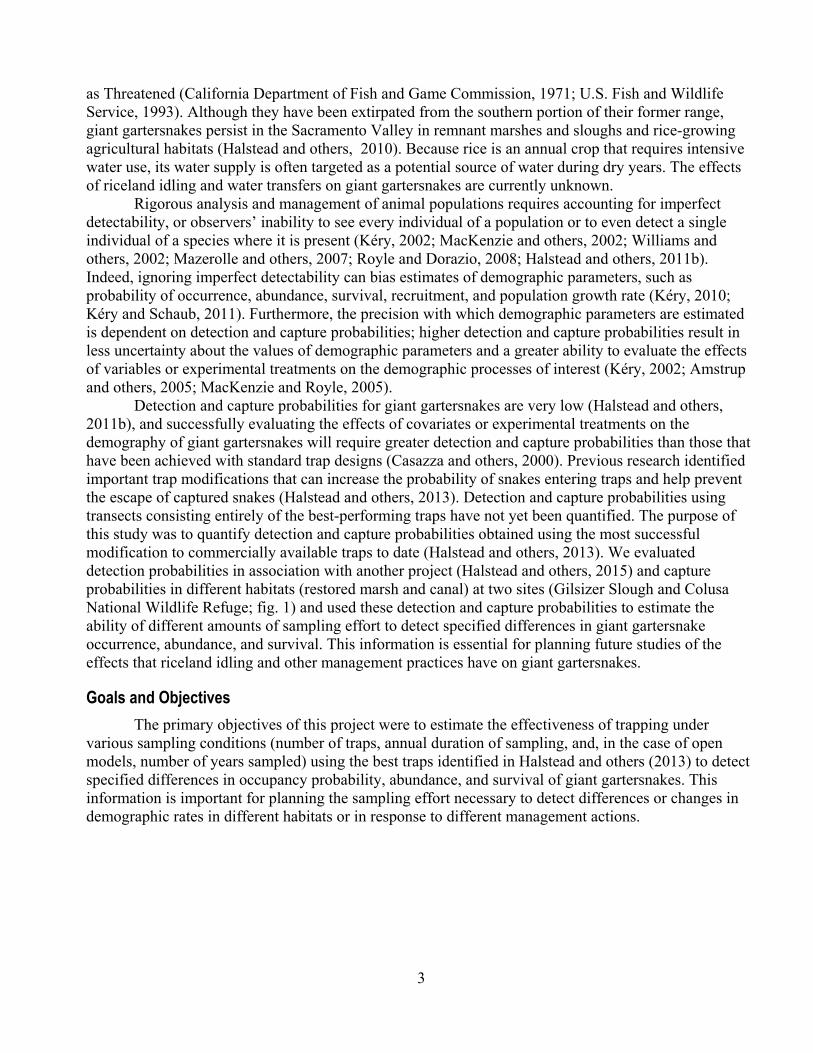
as Threatened (California Department of Fish and Game Commission, 1971; U.S. Fish and Wildlife Service, 1993). Although they have been extirpated from the southern portion of their former range, giant gartersnakes persist in the Sacramento Valley in remnant marshes and sloughs and rice-growing agricultural habitats (Halstead and others, 2010). Because rice is an annual crop that requires intensive water use, its water supply is often targeted as a potential source of water during dry years. The effects of riceland idling and water transfers on giant gartersnakes are currently unknown.

Rigorous analysis and management of animal populations requires accounting for imperfect detectability, or observers’ inability to see every individual of a population or to even detect a single individual of a species where it is present (Kéry, 2002; MacKenzie and others, 2002; Williams and others, 2002; Mazerolle and others, 2007; Royle and Dorazio, 2008; Halstead and others, 2011b). Indeed, ignoring imperfect detectability can bias estimates of demographic parameters, such as probability of occurrence, abundance, survival, recruitment, and population growth rate (Kéry, 2010; Kéry and Schaub, 2011). Furthermore, the precision with which demographic parameters are estimated is dependent on detection and capture probabilities; higher detection and capture probabilities result in less uncertainty about the values of demographic parameters and a greater ability to evaluate the effects of variables or experimental treatments on the demographic processes of interest (Kéry, 2002; Amstrup and others, 2005; MacKenzie and Royle, 2005).

Detection and capture probabilities for giant gartersnakes are very low (Halstead and others, 2011b), and successfully evaluating the effects of covariates or experimental treatments on the demography of giant gartersnakes will require greater detection and capture probabilities than those that have been achieved with standard trap designs (Casazza and others, 2000). Previous research identified important trap modifications that can increase the probability of snakes entering traps and help prevent the escape of captured snakes (Halstead and others, 2013). Detection and capture probabilities using transects consisting entirely of the best-performing traps have not yet been quantified. The purpose of this study was to quantify detection and capture probabilities obtained using the most successful modification to commercially available traps to date (Halstead and others, 2013). We evaluated detection probabilities in association with another project (Halstead and others, 2015) and capture probabilities in different habitats (restored marsh and canal) at two sites (Gilsizer Slough and Colusa National Wildlife Refuge; fig. 1) and used these detection and capture probabilities to estimate the ability of different amounts of sampling effort to detect specified differences in giant gartersnake occurrence, abundance, and survival. This information is essential for planning future studies of the effects that riceland idling and other management practices have on giant gartersnakes.

Goals and Objectives The primary objectives of this project were to estimate the effectiveness of trapping under

various sampling conditions (number of traps, annual duration of sampling, and, in the case of open models, number of years sampled) using the best traps identified in Halstead and others (2013) to detect specified differences in occupancy probability, abundance, and survival of giant gartersnakes. This information is important for planning the sampling effort necessary to detect differences or changes in demographic rates in different habitats or in response to different management actions.

4

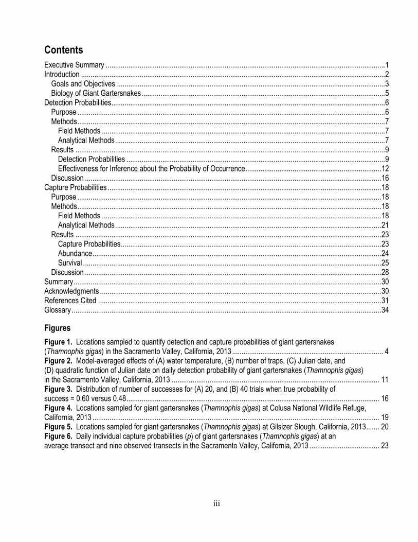
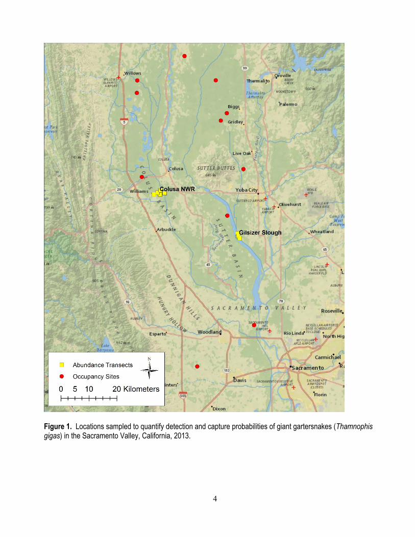
Figure 1. Locations sampled to quantify detection and capture probabilities of giant gartersnakes (Thamnophis gigas) in the Sacramento Valley, California, 2013.

5

Biology of Giant Gartersnakes Giant gartersnakes are precinctive to wetlands in California’s Central Valley. They were first

described in the southern San Joaquin Valley by Fitch (1940) as a subspecies of the aquatic gartersnake (at that time, Thamnophis ordinoides). Further taxonomic revisions resulted in the consideration of the giant gartersnake as a subspecies of the sierra gartersnake (Thamnophis couchii). Because giant gartersnakes are morphologically distinguishable from and do not occur at the same locations as their most closely related species, aquatic gartersnakes (Thamnophis atratus) and sierra gartersnakes, they were recognized as a full species in 1987 (Rossman and Stewart, 1987).

Giant gartersnakes are highly aquatic and historically occurred in marshes, sloughs, and other habitats with slow-moving, relatively warm water and emergent vegetation, especially tules (Schoenoplectus [Scirpus] acutus). Although conversion of wetlands to agriculture has nearly extirpated giant gartersnakes from the San Joaquin Valley, this species persists in remnant marshes and sloughs and rice agriculture in the Sacramento Valley (Halstead and others, 2010). Canals associated with rice agriculture can provide marsh-like habitat conditions throughout the active season of giant gartersnakes (late March–early October; Wylie and others, 2009), and rice fields are emergent wetlands for a part of the active season.

Giant gartersnakes feed primarily on small fish, frogs, and tadpoles (Rossman and others, 1996). Specific prey include tadpoles and small adults of American bullfrogs (Lithobates catesbeianus) and tadpoles and adults of sierran treefrogs (Pseudacris sierra). Fish prey include but are not limited to mosquitofish (Gambusia affinis) and small cyprinid (Cyprinidae spp.) and centrarchid (Centrarchidae spp.) fishes. Little is known about the diet of juvenile giant gartersnakes.

Giant gartersnakes are the longest species of gartersnake (Rossman and others, 1996). Like most natricine (Natricinae spp.) snakes, giant gartersnakes are sexually dimorphic in size, with females the larger sex (Wylie and others, 2010). Like most reptiles, small giant gartersnakes grow faster than large giant gartersnakes (Coates and others, 2009). Males and females exhibit differing seasonal growth patterns, with males forgoing foraging (and growth) for reproductive opportunities in the early spring (Coates and others, 2009). Similarly, male body condition is much lower than female body condition during the spring mating season, but males and females enter brumation in similar condition (Coates and others, 2009). Body condition might be related to the thermal ecology of giant gartersnakes. Female giant gartersnakes exhibit elevated body temperatures during June, July, and August (Wylie and others, 2009), which is the period during which they are gravid. In contrast, males exhibit elevated body temperature in the winter and early spring (Wylie and others, 2009), likely to prepare for the spring mating season. Elevated body temperature of males might be metabolically costly, causing decreased body condition for male snakes in spring.

Although some aspects of the demography of giant gartersnakes are difficult to determine, detailed study of populations in the Sacramento Valley has yielded some insight into their population ecology. Giant gartersnakes in the Sacramento Valley tend to produce smaller litters than those historically observed in the San Joaquin Valley. In the San Joaquin Valley, mean litter size was 23 (standard deviation=9.06; Hansen and Hansen, 1990). In the Sacramento Valley, mean litter size was 17 (95-percent confidence interval [CI] = 13–21; Halstead and others, 2011a). Mean parturition date was August 13, although parturition can occur from early July through early October (Halstead and others, 2011a). Neonates in the Sacramento Valley are born at a mean snout-vent length (SVL) of about 209 mm and a mean mass of about 4.9 g (Halstead and others, 2011a). Litter size varies interannually, is potentially linked to resource availability, and large females produce more, rather than larger, offspring (Halstead and others, 2011a).

6

Survival of adult female giant gartersnakes in the Sacramento Valley varies among sites and 14 years (1995‒2002 and 2004‒2009). At an average site in an average year, annual survival probability of adult females greater than 180 g was 0.61 (95-percent credible interval [CRI] = 0.41–0.79; Halstead and others, 2012). Individuals are at 2.6 times (1.1–11.1) greater daily risk of mortality in aquatic habitats than in terrestrial habitats (Halstead and others, 2012), likely because most terrestrial locations occur when snakes are in subterranean refuges such as under vegetation or in burrows. The effect of linear habitats (that is, canals or streams) on daily risk of mortality varied with context; in rice-growing agricultural systems, daily risk of mortality was less in canals than away from canals, but in systems with natural or restored marshes, risk of mortality was less in these two-dimensional habitats than in simple linear canals (Halstead and others, 2012). Overall survival was greatest in a site with a relatively large network of restored marshes (Halstead and others, 2012).

Abundance, density, and body condition of giant gartersnakes vary by site, presumably as a result of differences in habitat between sites. Abundances and densities were greatest in a natural wetland, less in a natural wetland modified for agricultural uses, less still in rice agriculture, and least in seasonal marshes managed for waterfowl (moist soil management in summer, flooded in winter; Wylie and others, 2010). Body condition of females followed a similar pattern (Wylie and others, 2010). Habitats that resemble natural marshes, therefore, are most likely to support dense populations of healthy giant gartersnakes.

Prior to settlement, the range of giant gartersnakes extended from Butte County in the north to Kern County in the south (Fitch, 1940; Hansen and Brode, 1980). The draining of wetlands and subsequent urban and agricultural development contributed to the loss of more than 90 percent of wetlands in the Central Valley (Frayer and others, 1989). The few remaining natural wetlands are fragmented and the natural cycle of seasonal valley flooding by High Sierra snowmelt has been limited as water presently is diverted by a network of dams and levees. As a result, giant gartersnake populations have become fragmented, with only small isolated populations remaining in the San Joaquin Valley. These factors precipitated the listing of giant gartersnakes by the State of California (California Department of Fish and Game Commission 1971), and later by the U.S. Fish and Wildlife Service as a threatened species with a recovery priority designation of 2C: full species, high degree of threat, and high recovery potential (U.S. Fish and Wildlife Service, 1993, 1999).

Detection Probabilities Purpose

Low detection probabilities result in greater uncertainty about whether giant gartersnakes are absent from a site, or are merely undetected during surveys. This uncertainty propagates to inferences about the probability of occurrence of giant gartersnakes and makes uncertain any evaluation of the effects of covariates on occupancy, colonization, or extirpation probabilities. Daily detection probabilities (p) for giant gartersnakes using floating aquatic funnel traps without further modifications (Casazza and others, 2000) are very low (Halstead and others, 2011b), and successfully evaluating the effects of covariates or experimental treatments on the probability of occurrence of giant gartersnakes would benefit from increased p. We therefore quantified detection probabilities using the best-performing modified floating aquatic funnel traps identified in Halstead and others (2013), and used these detection probabilities to estimate the ability of current field methods to detect differences in occupancy probabilities of giant gartersnakes.

7

Methods

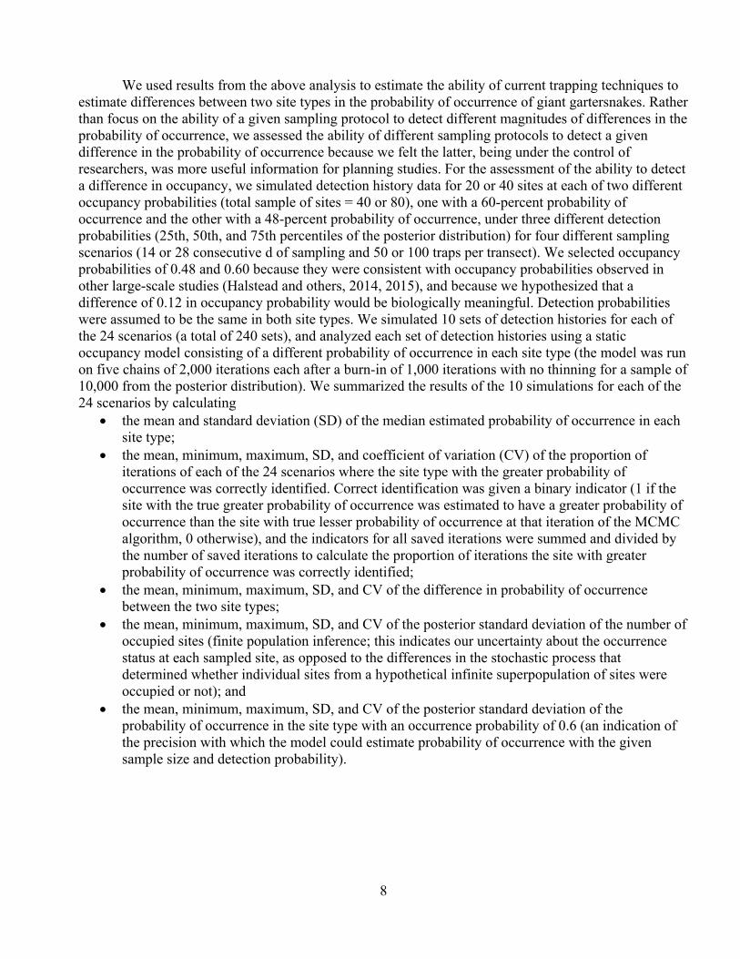
Field Methods We deployed two transects of 50 traps each at 11 sites in the Sacramento Valley between June 14

and September 13, 2013, to quantify detection probabilities (fig. 1). All traps were constructed of galvanized hardware cloth modified to have funnel extensions and one-way valves (Halstead and others, 2013). Within sites, we placed transects based on landowner permission and field observations of habitat so as to maximize the likelihood of detecting giant gartersnakes. We positioned transects along the banks of canals or at the edge of emergent vegetation in wetlands because giant gartersnakes forage along habitat edges and habitat edges also act as natural drift fences that direct snake movement to traps. The traps remained deployed and were checked daily until we captured a giant gartersnake and had another site identified at which to deploy traps, or we reached the target 21 day deployment duration, whichever came first.

Analytical Methods We calculated detection probabilities of giant gartersnakes using Bayesian analysis of static

occupancy models (Kéry, 2002, 2010; MacKenzie and others, 2002, 2006). For this analysis, we fit a full model containing effects of air and water temperatures, the difference between air and water temperatures, daily number of traps, date, and a quadratic function of date on daily detection probability. Although previous studies have found heterogeneity among sites in detection probability (Halstead and others, 2011b), we did not include site-level heterogeneity because of our small sample size. We fit a model with constant probability of occurrence because we were not interested in this parameter for this analysis. We standardized all continuous variables to a mean of 0 and variance of 1 to improve behavior of the Markov chain Monte Carlo (MCMC) algorithm. We calculated the posterior probability of each subset of the full model using indicator variables on model parameters (Kuo and Mallick, 1998; Royle and Dorazio, 2008). In this approach to model selection, a predictor is included in the model when the indicator variable for that predictor has a value of 1, and is excluded from the model when the indicator variable for that predictor has a value of 0. Each unique sequence of indicator variables specifies the full model (all 1s) or some subset of it. The proportion of iterations for which each unique sequence of indicator variables (specifying a specific model) occurs is that model’s posterior probability. We used uninformative priors for all parameters of the model: Beta(1,1) for probabilities, N(0,1.648) (mean, standard deviation) for regression coefficients (which is approximately uniform when transformed from the logit scale to the probability scale), U(0,10) for standard deviations, and Bin(1,0.5) for indicator variables.

We used standard MCMC algorithms to obtain posterior inference from the models. Each model was run on five chains of 10,000 iterations each after a burn-in period of 10,000 iterations; each chain was thinned by a factor of five, resulting in posterior inference based on 10,000 samples from the stationary posterior distribution. We assessed convergence with history plots and found no evidence for lack of convergence. We analyzed each model using JAGS 3.3.0 (Plummer, 2014a) via R 3.2.0 (R Core Team, 2014) with the R package rjags (Plummer, 2014b). Unless otherwise indicated, results are presented as the posterior median and 95-percent credible interval (CRI).

8

We used results from the above analysis to estimate the ability of current trapping techniques to estimate differences between two site types in the probability of occurrence of giant gartersnakes. Rather than focus on the ability of a given sampling protocol to detect different magnitudes of differences in the probability of occurrence, we assessed the ability of different sampling protocols to detect a given difference in the probability of occurrence because we felt the latter, being under the control of researchers, was more useful information for planning studies. For the assessment of the ability to detect a difference in occupancy, we simulated detection history data for 20 or 40 sites at each of two different occupancy probabilities (total sample of sites = 40 or 80), one with a 60-percent probability of occurrence and the other with a 48-percent probability of occurrence, under three different detection probabilities (25th, 50th, and 75th percentiles of the posterior distribution) for four different sampling scenarios (14 or 28 consecutive d of sampling and 50 or 100 traps per transect). We selected occupancy probabilities of 0.48 and 0.60 because they were consistent with occupancy probabilities observed in other large-scale studies (Halstead and others, 2014, 2015), and because we hypothesized that a difference of 0.12 in occupancy probability would be biologically meaningful. Detection probabilities were assumed to be the same in both site types. We simulated 10 sets of detection histories for each of the 24 scenarios (a total of 240 sets), and analyzed each set of detection histories using a static occupancy model consisting of a different probability of occurrence in each site type (the model was run on five chains of 2,000 iterations each after a burn-in of 1,000 iterations with no thinning for a sample of 10,000 from the posterior distribution). We summarized the results of the 10 simulations for each of the 24 scenarios by calculating

• the mean and standard deviation (SD) of the median estimated probability of occurrence in each site type;

• the mean, minimum, maximum, SD, and coefficient of variation (CV) of the proportion of iterations of each of the 24 scenarios where the site type with the greater probability of occurrence was correctly identified. Correct identification was given a binary indicator (1 if the site with the true greater probability of occurrence was estimated to have a greater probability of occurrence than the site with true lesser probability of occurrence at that iteration of the MCMC algorithm, 0 otherwise), and the indicators for all saved iterations were summed and divided by the number of saved iterations to calculate the proportion of iterations the site with greater probability of occurrence was correctly identified;

• the mean, minimum, maximum, SD, and CV of the difference in probability of occurrence between the two site types;

• the mean, minimum, maximum, SD, and CV of the posterior standard deviation of the number of occupied sites (finite population inference; this indicates our uncertainty about the occurrence status at each sampled site, as opposed to the differences in the stochastic process that determined whether individual sites from a hypothetical infinite superpopulation of sites were occupied or not); and

• the mean, minimum, maximum, SD, and CV of the posterior standard deviation of the probability of occurrence in the site type with an occurrence probability of 0.6 (an indication of the precision with which the model could estimate probability of occurrence with the given sample size and detection probability).

9

Results

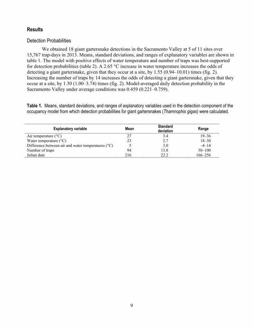
Detection Probabilities We obtained 18 giant gartersnake detections in the Sacramento Valley at 5 of 11 sites over

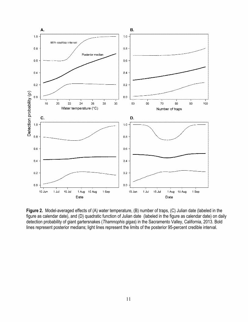
15,767 trap-days in 2013. Means, standard deviations, and ranges of explanatory variables are shown in table 1. The model with positive effects of water temperature and number of traps was best-supported for detection probabilities (table 2). A 2.65 °C increase in water temperature increases the odds of detecting a giant gartersnake, given that they occur at a site, by 1.55 (0.94–10.01) times (fig. 2). Increasing the number of traps by 14 increases the odds of detecting a giant gartersnake, given that they occur at a site, by 1.30 (1.00–3.74) times (fig. 2). Model-averaged daily detection probability in the Sacramento Valley under average conditions was 0.459 (0.221–0.759).

Table 1. Means, standard deviations, and ranges of explanatory variables used in the detection component of the occupancy model from which detection probabilities for giant gartersnakes (Thamnophis gigas) were calculated.

Explanatory variable Mean Standard deviation Range

Air temperature (°C) 27 3.4 19‒36 Water temperature (°C) 23 2.7 18‒30 Difference between air and water temperatures (°C) 5 3.0 -4‒14 Number of traps 94 13.8 50‒100 Julian date 216 22.2 166‒256

10

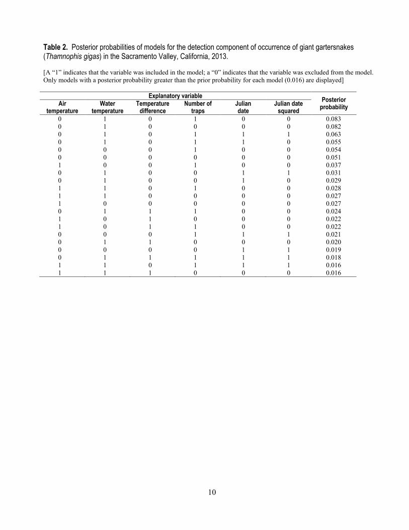
Table 2. Posterior probabilities of models for the detection component of occurrence of giant gartersnakes (Thamnophis gigas) in the Sacramento Valley, California, 2013. [A “1” indicates that the variable was included in the model; a “0” indicates that the variable was excluded from the model. Only models with a posterior probability greater than the prior probability for each model (0.016) are displayed]

Explanatory variable Posterior probability Air

temperature Water

temperature Temperature

difference Number of

traps Julian date

Julian date squared

0 1 0 1 0 0 0.083 0 1 0 0 0 0 0.082 0 1 0 1 1 1 0.063 0 1 0 1 1 0 0.055 0 0 0 1 0 0 0.054 0 0 0 0 0 0 0.051 1 0 0 1 0 0 0.037 0 1 0 0 1 1 0.031 0 1 0 0 1 0 0.029 1 1 0 1 0 0 0.028 1 1 0 0 0 0 0.027 1 0 0 0 0 0 0.027 0 1 1 1 0 0 0.024 1 0 1 0 0 0 0.022 1 0 1 1 0 0 0.022 0 0 0 1 1 1 0.021 0 1 1 0 0 0 0.020 0 0 0 0 1 1 0.019 0 1 1 1 1 1 0.018 1 1 0 1 1 1 0.016 1 1 1 0 0 0 0.016

11

Figure 2. Model-averaged effects of (A) water temperature, (B) number of traps, (C) Julian date (labeled in the figure as calendar date), and (D) quadratic function of Julian date (labeled in the figure as calendar date) on daily detection probability of giant gartersnakes (Thamnophis gigas) in the Sacramento Valley, California, 2013. Bold lines represent posterior medians; light lines represent the limits of the posterior 95-percent credible interval.

12

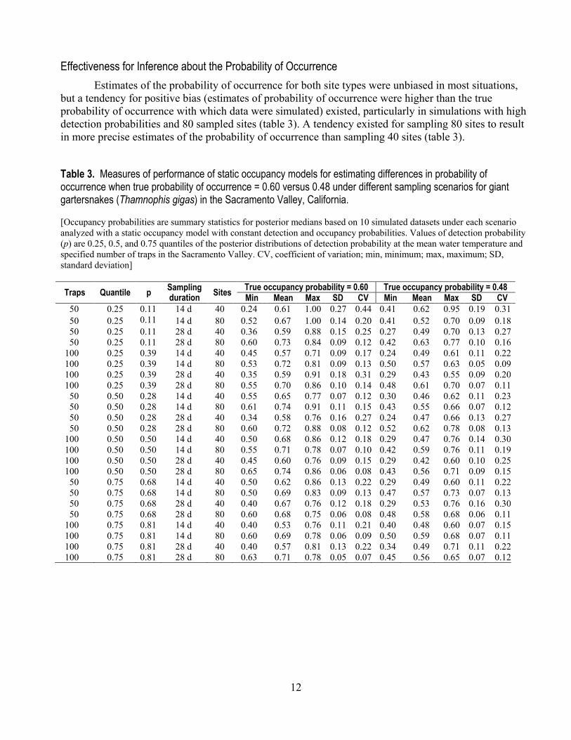
Effectiveness for Inference about the Probability of Occurrence Estimates of the probability of occurrence for both site types were unbiased in most situations,

but a tendency for positive bias (estimates of probability of occurrence were higher than the true probability of occurrence with which data were simulated) existed, particularly in simulations with high detection probabilities and 80 sampled sites (table 3). A tendency existed for sampling 80 sites to result in more precise estimates of the probability of occurrence than sampling 40 sites (table 3).

Table 3. Measures of performance of static occupancy models for estimating differences in probability of occurrence when true probability of occurrence = 0.60 versus 0.48 under different sampling scenarios for giant gartersnakes (Thamnophis gigas) in the Sacramento Valley, California. [Occupancy probabilities are summary statistics for posterior medians based on 10 simulated datasets under each scenario analyzed with a static occupancy model with constant detection and occupancy probabilities. Values of detection probability (p) are 0.25, 0.5, and 0.75 quantiles of the posterior distributions of detection probability at the mean water temperature and specified number of traps in the Sacramento Valley. CV, coefficient of variation; min, minimum; max, maximum; SD, standard deviation]

Traps Quantile p Sampling duration Sites True occupancy probability = 0.60 True occupancy probability = 0.48

Min Mean Max SD CV Min Mean Max SD CV 50 0.25 0.11 14 d 40 0.24 0.61 1.00 0.27 0.44 0.41 0.62 0.95 0.19 0.31 50 0.25 0.11 14 d 80 0.52 0.67 1.00 0.14 0.20 0.41 0.52 0.70 0.09 0.18 50 0.25 0.11 28 d 40 0.36 0.59 0.88 0.15 0.25 0.27 0.49 0.70 0.13 0.27 50 0.25 0.11 28 d 80 0.60 0.73 0.84 0.09 0.12 0.42 0.63 0.77 0.10 0.16

100 0.25 0.39 14 d 40 0.45 0.57 0.71 0.09 0.17 0.24 0.49 0.61 0.11 0.22 100 0.25 0.39 14 d 80 0.53 0.72 0.81 0.09 0.13 0.50 0.57 0.63 0.05 0.09 100 0.25 0.39 28 d 40 0.35 0.59 0.91 0.18 0.31 0.29 0.43 0.55 0.09 0.20 100 0.25 0.39 28 d 80 0.55 0.70 0.86 0.10 0.14 0.48 0.61 0.70 0.07 0.11 50 0.50 0.28 14 d 40 0.55 0.65 0.77 0.07 0.12 0.30 0.46 0.62 0.11 0.23 50 0.50 0.28 14 d 80 0.61 0.74 0.91 0.11 0.15 0.43 0.55 0.66 0.07 0.12 50 0.50 0.28 28 d 40 0.34 0.58 0.76 0.16 0.27 0.24 0.47 0.66 0.13 0.27 50 0.50 0.28 28 d 80 0.60 0.72 0.88 0.08 0.12 0.52 0.62 0.78 0.08 0.13

100 0.50 0.50 14 d 40 0.50 0.68 0.86 0.12 0.18 0.29 0.47 0.76 0.14 0.30 100 0.50 0.50 14 d 80 0.55 0.71 0.78 0.07 0.10 0.42 0.59 0.76 0.11 0.19 100 0.50 0.50 28 d 40 0.45 0.60 0.76 0.09 0.15 0.29 0.42 0.60 0.10 0.25 100 0.50 0.50 28 d 80 0.65 0.74 0.86 0.06 0.08 0.43 0.56 0.71 0.09 0.15 50 0.75 0.68 14 d 40 0.50 0.62 0.86 0.13 0.22 0.29 0.49 0.60 0.11 0.22 50 0.75 0.68 14 d 80 0.50 0.69 0.83 0.09 0.13 0.47 0.57 0.73 0.07 0.13 50 0.75 0.68 28 d 40 0.40 0.67 0.76 0.12 0.18 0.29 0.53 0.76 0.16 0.30 50 0.75 0.68 28 d 80 0.60 0.68 0.75 0.06 0.08 0.48 0.58 0.68 0.06 0.11

100 0.75 0.81 14 d 40 0.40 0.53 0.76 0.11 0.21 0.40 0.48 0.60 0.07 0.15 100 0.75 0.81 14 d 80 0.60 0.69 0.78 0.06 0.09 0.50 0.59 0.68 0.07 0.11 100 0.75 0.81 28 d 40 0.40 0.57 0.81 0.13 0.22 0.34 0.49 0.71 0.11 0.22 100 0.75 0.81 28 d 80 0.63 0.71 0.78 0.05 0.07 0.45 0.56 0.65 0.07 0.12

13

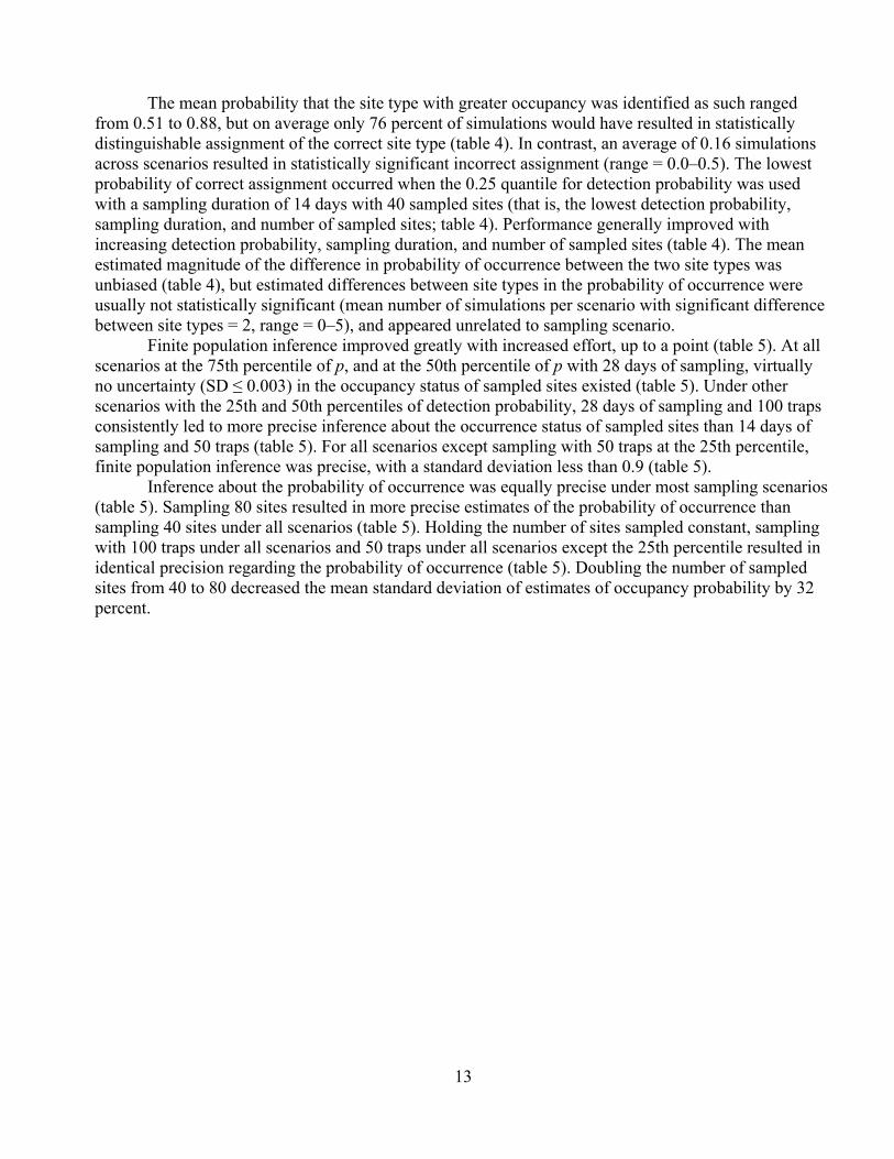
The mean probability that the site type with greater occupancy was identified as such ranged from 0.51 to 0.88, but on average only 76 percent of simulations would have resulted in statistically distinguishable assignment of the correct site type (table 4). In contrast, an average of 0.16 simulations across scenarios resulted in statistically significant incorrect assignment (range = 0.0‒0.5). The lowest probability of correct assignment occurred when the 0.25 quantile for detection probability was used with a sampling duration of 14 days with 40 sampled sites (that is, the lowest detection probability, sampling duration, and number of sampled sites; table 4). Performance generally improved with increasing detection probability, sampling duration, and number of sampled sites (table 4). The mean estimated magnitude of the difference in probability of occurrence between the two site types was unbiased (table 4), but estimated differences between site types in the probability of occurrence were usually not statistically significant (mean number of simulations per scenario with significant difference between site types = 2, range = 0‒5), and appeared unrelated to sampling scenario.

Finite population inference improved greatly with increased effort, up to a point (table 5). At all scenarios at the 75th percentile of p, and at the 50th percentile of p with 28 days of sampling, virtually no uncertainty (SD ≤ 0.003) in the occupancy status of sampled sites existed (table 5). Under other scenarios with the 25th and 50th percentiles of detection probability, 28 days of sampling and 100 traps consistently led to more precise inference about the occurrence status of sampled sites than 14 days of sampling and 50 traps (table 5). For all scenarios except sampling with 50 traps at the 25th percentile, finite population inference was precise, with a standard deviation less than 0.9 (table 5).

Inference about the probability of occurrence was equally precise under most sampling scenarios (table 5). Sampling 80 sites resulted in more precise estimates of the probability of occurrence than sampling 40 sites under all scenarios (table 5). Holding the number of sites sampled constant, sampling with 100 traps under all scenarios and 50 traps under all scenarios except the 25th percentile resulted in identical precision regarding the probability of occurrence (table 5). Doubling the number of sampled sites from 40 to 80 decreased the mean standard deviation of estimates of occupancy probability by 32 percent.

14

Table 4. Ability of occupancy models to detect a difference in probability of occurrence when true probability of occurrence = 0.60 versus 0.48 under different sampling scenarios for giant gartersnakes (Thamnophis gigas) in the Sacramento Valley, California. [Occupancy probabilities are summary statistics for posterior medians based on 10 simulated datasets under each scenario analyzed with a static occupancy model with constant detection and occupancy probabilities. Prop. sig. indicates the proportion of simulations for which the probability of correct assignment was better than expected by chance (0.51). Values of detection probability (p) are 0.25, 0.5, and 0.75 quantiles of the posterior distributions of detection probability at the mean water temperature and specified number of traps in the Sacramento Valley. CV, coefficient of variation; min, minimum; max, maximum; SD, standard deviation]

Sites p Sampling duration Sites

Proportion of iterations site type with greater occupancy correctly assigned

Estimated difference in probability of occurrence between site types (true value = 0.12)

Min. Mean Max. Prop. sig. Min. Mean Max. SD CV 50 0.11 14 d 40 0.02 0.51 0.94 0.5 -0.40 -0.01 0.36 0.28 30.08 50 0.11 14 d 80 0.24 0.77 1.00 0.8 -0.11 0.15 0.49 0.17 1.09 50 0.11 28 d 40 0.02 0.64 1.00 0.6 -0.32 0.10 0.60 0.24 2.39 50 0.11 28 d 80 0.17 0.71 1.00 0.7 -0.11 0.10 0.38 0.13 1.38

100 0.39 14 d 40 0.26 0.63 0.99 0.6 -0.10 0.08 0.40 0.16 2.03 100 0.39 14 d 80 0.17 0.82 >0.99 0.9 -0.10 0.16 0.30 0.13 0.85 100 0.39 28 d 40 0.37 0.76 >0.99 0.9 -0.05 0.16 0.45 0.16 1.02 100 0.39 28 d 80 0.32 0.69 >0.99 0.6 -0.05 0.09 0.28 0.12 1.40 50 0.28 14 d 40 0.37 0.82 0.99 0.8 -0.05 0.18 0.36 0.13 0.70 50 0.28 14 d 80 0.31 0.88 1.00 0.9 -0.05 0.19 0.35 0.12 0.63 50 0.28 28 d 40 0.25 0.65 >0.99 0.6 -0.10 0.11 0.46 0.20 1.74 50 0.28 28 d 80 0.22 0.74 1.00 0.8 -0.08 0.11 0.30 0.13 1.18

100 0.50 14 d 40 0.50 0.85 >0.99 0.9 0.00 0.21 0.41 0.14 0.66 100 0.50 14 d 80 0.40 0.79 >0.99 0.8 -0.02 0.12 0.33 0.11 0.89 100 0.50 28 d 40 0.26 0.80 0.99 0.9 -0.10 0.17 0.35 0.14 0.84 100 0.50 28 d 80 0.40 0.85 >0.99 0.8 -0.03 0.17 0.28 0.12 0.70 50 0.68 14 d 40 0.36 0.71 >0.99 0.7 -0.06 0.13 0.45 0.16 1.26 50 0.68 14 d 80 0.14 0.79 0.99 0.9 -0.12 0.11 0.25 0.11 0.97 50 0.68 28 d 40 0.16 0.68 >0.99 0.6 -0.15 0.14 0.46 0.22 1.64 50 0.68 28 d 80 0.49 0.78 0.98 0.8 0.00 0.10 0.22 0.08 0.77

100 0.81 14 d 40 0.25 0.60 0.85 0.6 -0.11 0.05 0.15 0.09 1.92 100 0.81 14 d 80 0.24 0.76 0.99 0.9 -0.08 0.10 0.25 0.10 0.99 100 0.81 28 d 40 0.03 0.68 0.95 0.7 -0.30 0.08 0.26 0.17 2.03 100 0.81 28 d 80 0.59 0.86 >0.99 1.0 0.02 0.15 0.30 0.09 0.61

15

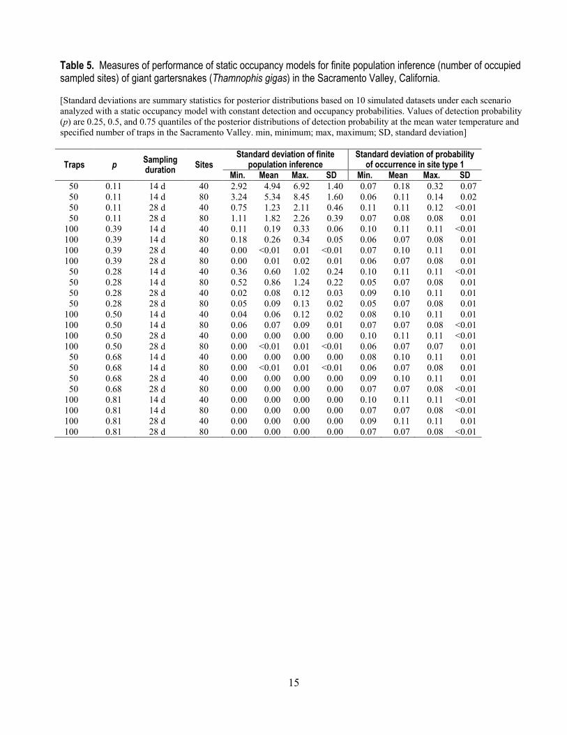
Table 5. Measures of performance of static occupancy models for finite population inference (number of occupied sampled sites) of giant gartersnakes (Thamnophis gigas) in the Sacramento Valley, California. [Standard deviations are summary statistics for posterior distributions based on 10 simulated datasets under each scenario analyzed with a static occupancy model with constant detection and occupancy probabilities. Values of detection probability (p) are 0.25, 0.5, and 0.75 quantiles of the posterior distributions of detection probability at the mean water temperature and specified number of traps in the Sacramento Valley. min, minimum; max, maximum; SD, standard deviation]

Traps p Sampling duration Sites

Standard deviation of finite population inference

Standard deviation of probability of occurrence in site type 1

Min. Mean Max. SD Min. Mean Max. SD 50 0.11 14 d 40 2.92 4.94 6.92 1.40 0.07 0.18 0.32 0.07 50 0.11 14 d 80 3.24 5.34 8.45 1.60 0.06 0.11 0.14 0.02 50 0.11 28 d 40 0.75 1.23 2.11 0.46 0.11 0.11 0.12 <0.01 50 0.11 28 d 80 1.11 1.82 2.26 0.39 0.07 0.08 0.08 0.01

100 0.39 14 d 40 0.11 0.19 0.33 0.06 0.10 0.11 0.11 <0.01 100 0.39 14 d 80 0.18 0.26 0.34 0.05 0.06 0.07 0.08 0.01 100 0.39 28 d 40 0.00 <0.01 0.01 <0.01 0.07 0.10 0.11 0.01 100 0.39 28 d 80 0.00 0.01 0.02 0.01 0.06 0.07 0.08 0.01 50 0.28 14 d 40 0.36 0.60 1.02 0.24 0.10 0.11 0.11 <0.01 50 0.28 14 d 80 0.52 0.86 1.24 0.22 0.05 0.07 0.08 0.01 50 0.28 28 d 40 0.02 0.08 0.12 0.03 0.09 0.10 0.11 0.01 50 0.28 28 d 80 0.05 0.09 0.13 0.02 0.05 0.07 0.08 0.01

100 0.50 14 d 40 0.04 0.06 0.12 0.02 0.08 0.10 0.11 0.01 100 0.50 14 d 80 0.06 0.07 0.09 0.01 0.07 0.07 0.08 <0.01 100 0.50 28 d 40 0.00 0.00 0.00 0.00 0.10 0.11 0.11 <0.01 100 0.50 28 d 80 0.00 <0.01 0.01 <0.01 0.06 0.07 0.07 0.01 50 0.68 14 d 40 0.00 0.00 0.00 0.00 0.08 0.10 0.11 0.01 50 0.68 14 d 80 0.00 <0.01 0.01 <0.01 0.06 0.07 0.08 0.01 50 0.68 28 d 40 0.00 0.00 0.00 0.00 0.09 0.10 0.11 0.01 50 0.68 28 d 80 0.00 0.00 0.00 0.00 0.07 0.07 0.08 <0.01

100 0.81 14 d 40 0.00 0.00 0.00 0.00 0.10 0.11 0.11 <0.01 100 0.81 14 d 80 0.00 0.00 0.00 0.00 0.07 0.07 0.08 <0.01 100 0.81 28 d 40 0.00 0.00 0.00 0.00 0.09 0.11 0.11 0.01 100 0.81 28 d 80 0.00 0.00 0.00 0.00 0.07 0.07 0.08 <0.01

16

Discussion Although inference about the difference in probability of occurrence between the two site types

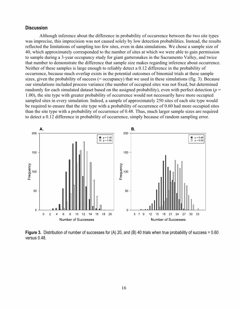
was imprecise, this imprecision was not caused solely by low detection probabilities. Instead, the results reflected the limitations of sampling too few sites, even in data simulations. We chose a sample size of 40, which approximately corresponded to the number of sites at which we were able to gain permission to sample during a 3-year occupancy study for giant gartersnakes in the Sacramento Valley, and twice that number to demonstrate the difference that sample size makes regarding inference about occurrence. Neither of these samples is large enough to reliably detect a 0.12 difference in the probability of occurrence, because much overlap exists in the potential outcomes of binomial trials at these sample sizes, given the probability of success (= occupancy) that we used in these simulations (fig. 3). Because our simulations included process variance (the number of occupied sites was not fixed, but determined randomly for each simulated dataset based on the assigned probability), even with perfect detection (p = 1.00), the site type with greater probability of occurrence would not necessarily have more occupied sampled sites in every simulation. Indeed, a sample of approximately 250 sites of each site type would be required to ensure that the site type with a probability of occurrence of 0.60 had more occupied sites than the site type with a probability of occurrence of 0.48. Thus, much larger sample sizes are required to detect a 0.12 difference in probability of occurrence, simply because of random sampling error.

Figure 3. Distribution of number of successes for (A) 20, and (B) 40 trials when true probability of success = 0.60 versus 0.48.

17

Because of this process error, conclusions drawn from the analysis of finite population inference are a more appropriate measure of trap performance than the analysis of inference about the probability of occurrence. Finite population inference refers to conclusions drawn about the specific sample, rather than to conclusions about the population from which the samples were drawn and to which inference is typically applied. In the context of this simulation study, it refers to the ability to determine how many sampled sites were occupied. Under all conditions at the 75th percentile of detection probability, and when sampling for 28 days at the median detection probability, regardless of sampling conditions, the 95-percent credible interval for the number of occupied sites was invariant. Indeed, finite population inference was precise for all sampling scenarios except sampling for 14 days at the 25th percentile of detection probability with 50 traps. Thus, our simulations clearly indicated that by using 100 modified traps for 2–4 weeks of sampling, one can distinguish occupied from unoccupied sites.

Because conclusions about occupancy are generally most useful when applied to the population of sites that could have been sampled, rather than just those sites that were actually sampled, it is instructive to consider inference to the larger population. In this case, nearly all scenarios (except for sampling with 50 traps for 14 days at the 25th percentile of detection probability) resulted in similar precision about the probability of occurrence, with a large sample of sites providing more precise estimates. Improvement in inference about the probability of occurrence of giant gartersnakes will therefore need to be achieved through an increase in the number of sampled sites, and not merely through increases in detection probabilities.

The primary limitation to these simulations is that they did not incorporate site-level heterogeneity in detection probability. Such heterogeneity is the norm, rather than the exception, for a number of reasons including site differences in abundance, thermal regimes, cover, individual behavior, habitat configuration, etc. Because we based our detection probabilities on only 11 sites, we were unable to account for heterogeneity among sites in detection probability. Nevertheless, our results suggest that using modified floating aquatic funnel traps (Casazza and others, 2000; Halstead and others, 2013) under the conditions examined will likely be sufficient for most applications related to inference about the probability of occurrence of giant gartersnakes, provided enough sites are sampled.

18

Capture Probabilities Purpose

Low capture probabilities result in increased uncertainty about the values of abundance, survival, and other demographic rates, and make uncertain any evaluation of the effects of variables or experimental treatments on population status and growth. Capture probabilities for giant gartersnakes are exceedingly low, and successfully evaluating the effects of environmental variables or experimental treatments on the demography of giant gartersnakes would benefit from increased capture probabilities. We therefore quantified capture probabilities using the best-performing traps identified in Halstead and others (2013), and used these capture probabilities to estimate the ability to detect differences in abundance and survival of giant gartersnakes.

Methods

Field Methods We sampled two sites, Colusa National Wildlife Refuge (NWR; fig. 4) and Gilsizer Slough (fig.

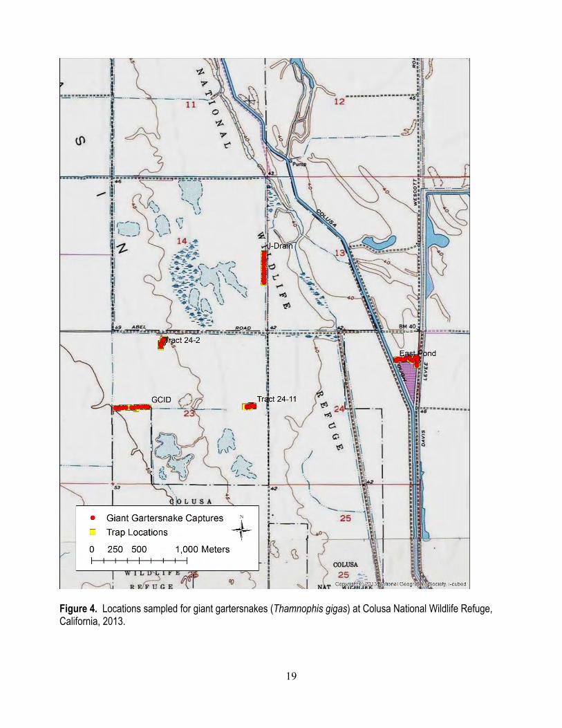
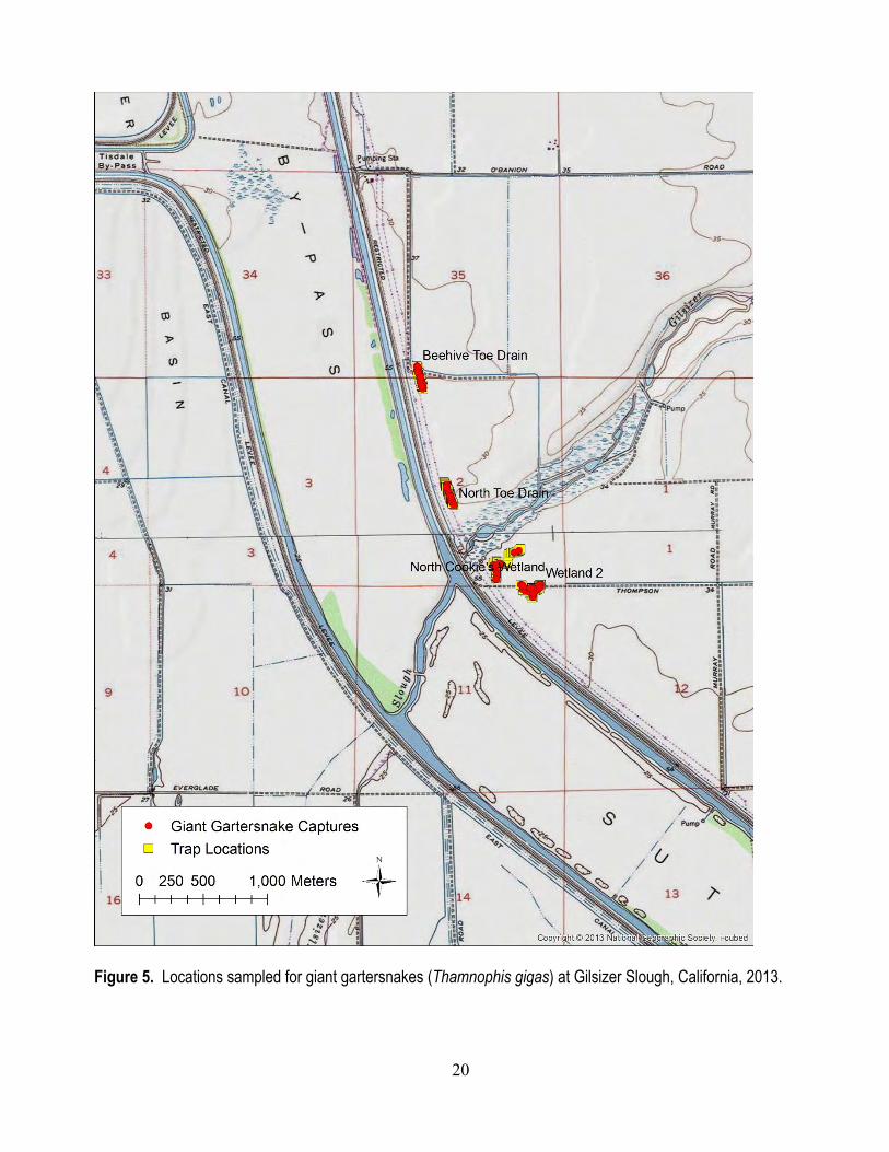
5) to quantify daily individual capture probabilities of giant gartersnakes. We deployed three transects of 50 traps each and two transects of 25 traps each at Colusa NWR, and four transects of 50 traps each at Gilsizer Slough. At each site, we placed two transects in canals (Colusa NWR: GCID Canal and J-Drain; Gilsizer Slough: Beehive Toe Drain and North Toe Drain) and two in created wetlands (Colusa NWR: Tract 24 and East Pond; Gilsizer Slough: North Cookies Wetland and Wetland 2) to sample habitats representative of most sampling conditions in the Sacramento Valley. At Colusa NWR, one of the wetland transects (Tract 24) had to be split among two units because of the small trappable area in the wetland units at this site. All traps were constructed of galvanized hardware cloth modified to have funnel extensions and one-way valves (Halstead and others, 2013). At Colusa NWR, we deployed traps on July 9, 2013, and checked them daily until they were removed on August 16, 2013. We deployed traps at Gilsizer Slough on May 24, 2013, and checked them daily until August 2, 2013, when all traps were removed. We marked each captured giant gartersnake with a unique brand (Winne and others, 2006) and passive integrated transponder (PIT) tag, and measured and determined the sex of each individual prior to releasing it at its location of capture.

19

Figure 4. Locations sampled for giant gartersnakes (Thamnophis gigas) at Colusa National Wildlife Refuge, California, 2013.

20

Figure 5. Locations sampled for giant gartersnakes (Thamnophis gigas) at Gilsizer Slough, California, 2013.

21

Analytical Methods We calculated capture probabilities of giant gartersnakes at each transect (we did not capture any

individual giant gartersnakes at more than one transect) using a hierarchical Bayesian analysis of closed population capture-mark-recapture models using data augmentation (Royle and Dorazio, 2008). Data augmentation is an approach to capture-mark-recapture analysis in which a large number of all zero capture histories, representing pseudo-individuals, is appended to the observed capture histories. From the combined sample of pseudo-individuals and observed individuals, the abundance estimation problem then becomes one of determining how many of the unobserved pseudo-individuals are members of the population that were not observed. The abundance estimation problem thus becomes analogous to the estimation of the probability of occurrence using occupancy models, with individuals analogous to sites. We conducted a preliminary analysis that allowed for hierarchical effects of the number of traps, sex, an ephemeral behavioral response, temporal heterogeneity, and individual heterogeneity. We did not use the results of these models because the credible intervals for all means and most individual sites overlapped zero. The exception to this pattern was individual heterogeneity, which was supported for some sites. Because individual heterogeneity models could not be fit for all sites, even using hierarchical models, we used a hierarchical model for which capture probability was constant over time and for all individuals within a site, but was allowed to vary among sites. We augmented the capture histories of trapped individuals at each site so that the total number of observed individuals plus unobserved pseudo-individuals was 200. We determined that the number of pseudo-individuals was adequate by the posterior densities falling far below the upper limit for abundance. We used uninformative priors for all parameters of the model: U(0,1) for probabilities, N(0,1.648) for the logit-scale intercept representing mean capture probability across sites, and U(0,5) for standard deviations.

We used standard MCMC algorithms to obtain posterior inference from the model. The model was run on five chains of 50,000 iterations each after a burn-in period of 2,000 iterations; each chain was thinned by a factor of 25, resulting in posterior inference based on 10,000 samples from the posterior distribution. We assessed convergence using the Gelman-Rubin statistic (Gelman and Rubin, 1992) and history plots and found no evidence for lack of convergence (𝑅� < 1.01 for all monitored parameters). We analyzed each model using JAGS 3.4.0 (Plummer, 2014a) via R 3.3.0 (R Core Team, 2014) with the R package runjags (M.J. Denwood, written commun.). Unless otherwise indicated, results are presented as the posterior median and 95-percent CRI.

We used results from the above analysis to evaluate the ability of trapping techniques to estimate differences among sites in abundance and survival. To do this, we sampled from the posterior distribution of the logit-scale intercept (mean capture probability across sites) and standard deviation from the abundance model and simulated the capture probability for each site from this distribution (that is, we used a posterior predictive distribution for capture probability at an unknown site). Rather than focus on the ability of a given sampling protocol to detect different magnitudes of differences in abundance, we assessed the ability of different sampling protocols to detect a given difference in abundance because we felt the latter, being under the control of researchers, was more useful information for planning studies. For the assessment of the ability to detect a difference in abundance, we simulated capture history data for two different populations, one with 100 individuals and one with 80 individuals under three different sampling scenarios (30, 60, and 90 consecutive days of sampling).

22

We selected abundances of 100 and 80 because they were consistent with abundances measured in previous studies (Wylie and others, 2010), and because we hypothesized that a difference of 20 individuals would be an important distinction among sites. We simulated 100 sets of capture histories under each scenario (a total of 300 simulated datasets for each population) and analyzed each set of capture histories using a separate simple constant capture probability closed model of abundance for each population (each capture history was augmented by 100 pseudo-individuals, then the model was run on five chains of 10,000 iterations each after a burn-in of 2,000 iterations and thinned by a factor of five for a sample of 10,000 from the posterior distribution). We summarized the results of the 100 iterations for each of the three scenarios by calculating the mean, median, minimum, maximum, and 95 percent CRI of the estimated capture probability and abundance for each population and difference in abundance and proportion difference in abundance between populations; the mean, median, minimum, and maximum, and 95-percent CRI of the proportion of iterations of each simulation where the population with greater abundance was correctly identified (based on whether abundance of the population with the greater number of individuals was estimated to be greater than the abundance of the other population at each iteration); and the proportion of these proportions that was greater than expected by chance (0.510, based on Bin(p = 0.5, N = 10,000)).

As for occupancy and abundance analyses, we assessed the ability of different sampling protocols to detect a given difference in survival because we felt that sampling protocols, being under the control of researchers, was more useful information for planning studies than hypothesized differences in survival. To assess the ability to detect a difference in survival, we simulated capture history data for two different populations, one with a constant annual survival probability of 0.70 and the other with a constant annual survival probability of 0.50 for three different sampling scenarios (30, 60, and 90 consecutive days of sampling within a year), with two different numbers of newly marked individuals each year (25 and 50), and for two different study durations (3 and 5 years). We selected annual survival probabilities of 0.70 and 0.50 because these values were consistent with annual survival probabilities of adult female giant gartersnakes (Halstead and others, 2012), and we hypothesized that a difference in annual survival probability of 0.20 would have biologically meaningful effects on giant gartersnake populations. We simulated 100 sets of capture histories under each scenario using the posterior predictive distribution for daily individual capture probability as above for abundance estimation (a total of 1,200 simulated datasets) and analyzed each set of capture histories using a separate simple constant survival and recapture probability Cormack-Jolly-Seber model for each population (the model was run on five chains of 10,000 iterations each after a burn-in of 2,000 iterations, thinned by a factor of 5 for a sample of 10,000 from the posterior distribution). We summarized the results of the 100 iterations for each of the 12 scenarios by calculating the mean, median, minimum, maximum, and 95-percent CRI of the estimated capture probability and annual survival probability for each population, and difference in annual probability of survival and proportion difference in annual probability of survival between populations; the mean, median, minimum, and maximum, and 95-percent CRI of the proportion of iterations of each simulation where the population with greater annual probability of survival was correctly identified (based on whether annual survival probability of the population with the greater survival rate was estimated to be greater than the annual survival probability of the other population at each iteration); and the proportion of these proportions that was greater than expected by chance (0.510, based on Bin(p = 0.5, N = 10,000)).

23

Results

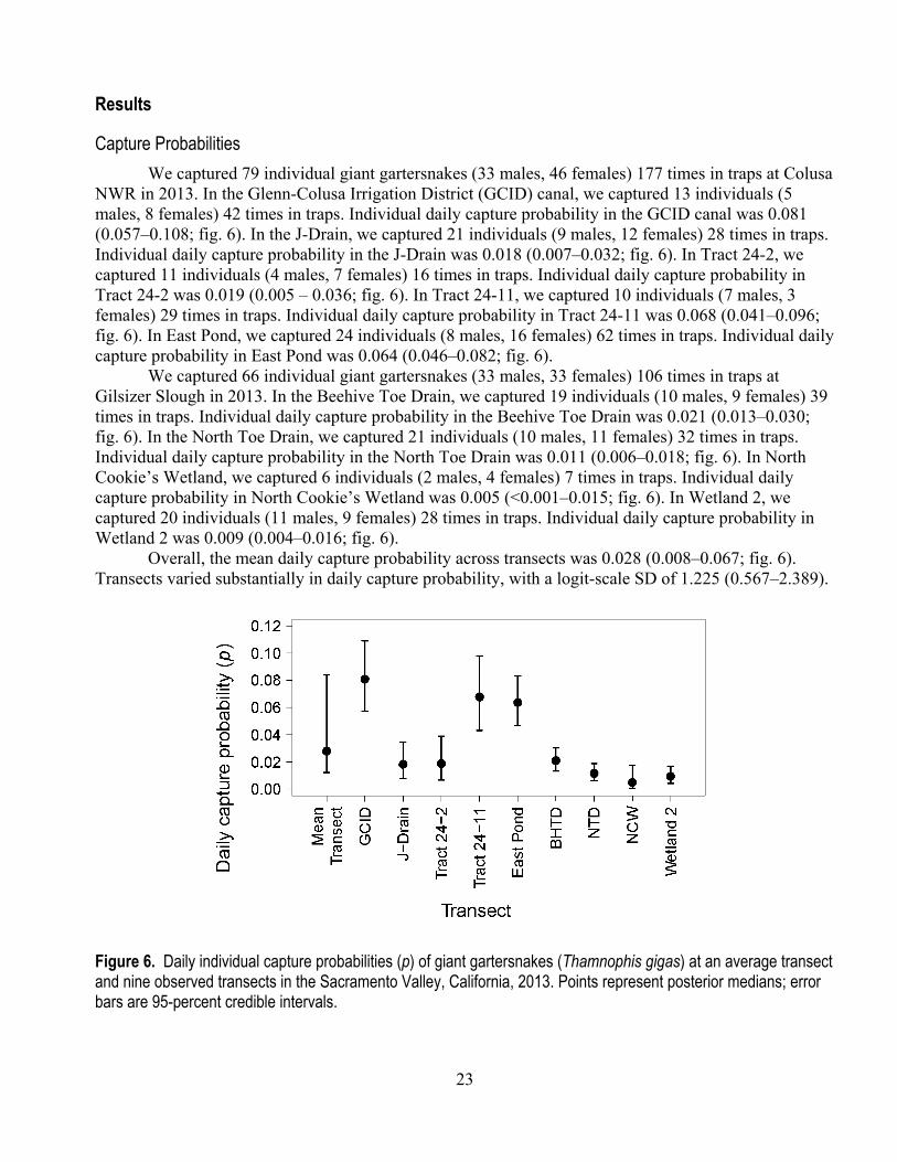
Capture Probabilities We captured 79 individual giant gartersnakes (33 males, 46 females) 177 times in traps at Colusa

NWR in 2013. In the Glenn-Colusa Irrigation District (GCID) canal, we captured 13 individuals (5 males, 8 females) 42 times in traps. Individual daily capture probability in the GCID canal was 0.081 (0.057–0.108; fig. 6). In the J-Drain, we captured 21 individuals (9 males, 12 females) 28 times in traps. Individual daily capture probability in the J-Drain was 0.018 (0.007–0.032; fig. 6). In Tract 24-2, we captured 11 individuals (4 males, 7 females) 16 times in traps. Individual daily capture probability in Tract 24-2 was 0.019 (0.005 – 0.036; fig. 6). In Tract 24-11, we captured 10 individuals (7 males, 3 females) 29 times in traps. Individual daily capture probability in Tract 24-11 was 0.068 (0.041–0.096; fig. 6). In East Pond, we captured 24 individuals (8 males, 16 females) 62 times in traps. Individual daily capture probability in East Pond was 0.064 (0.046–0.082; fig. 6).

We captured 66 individual giant gartersnakes (33 males, 33 females) 106 times in traps at Gilsizer Slough in 2013. In the Beehive Toe Drain, we captured 19 individuals (10 males, 9 females) 39 times in traps. Individual daily capture probability in the Beehive Toe Drain was 0.021 (0.013–0.030; fig. 6). In the North Toe Drain, we captured 21 individuals (10 males, 11 females) 32 times in traps. Individual daily capture probability in the North Toe Drain was 0.011 (0.006–0.018; fig. 6). In North Cookie’s Wetland, we captured 6 individuals (2 males, 4 females) 7 times in traps. Individual daily capture probability in North Cookie’s Wetland was 0.005 (<0.001–0.015; fig. 6). In Wetland 2, we captured 20 individuals (11 males, 9 females) 28 times in traps. Individual daily capture probability in Wetland 2 was 0.009 (0.004–0.016; fig. 6).

Overall, the mean daily capture probability across transects was 0.028 (0.008‒0.067; fig. 6). Transects varied substantially in daily capture probability, with a logit-scale SD of 1.225 (0.567‒2.389).

Figure 6. Daily individual capture probabilities (p) of giant gartersnakes (Thamnophis gigas) at an average transect and nine observed transects in the Sacramento Valley, California, 2013. Points represent posterior medians; error bars are 95-percent credible intervals.

24

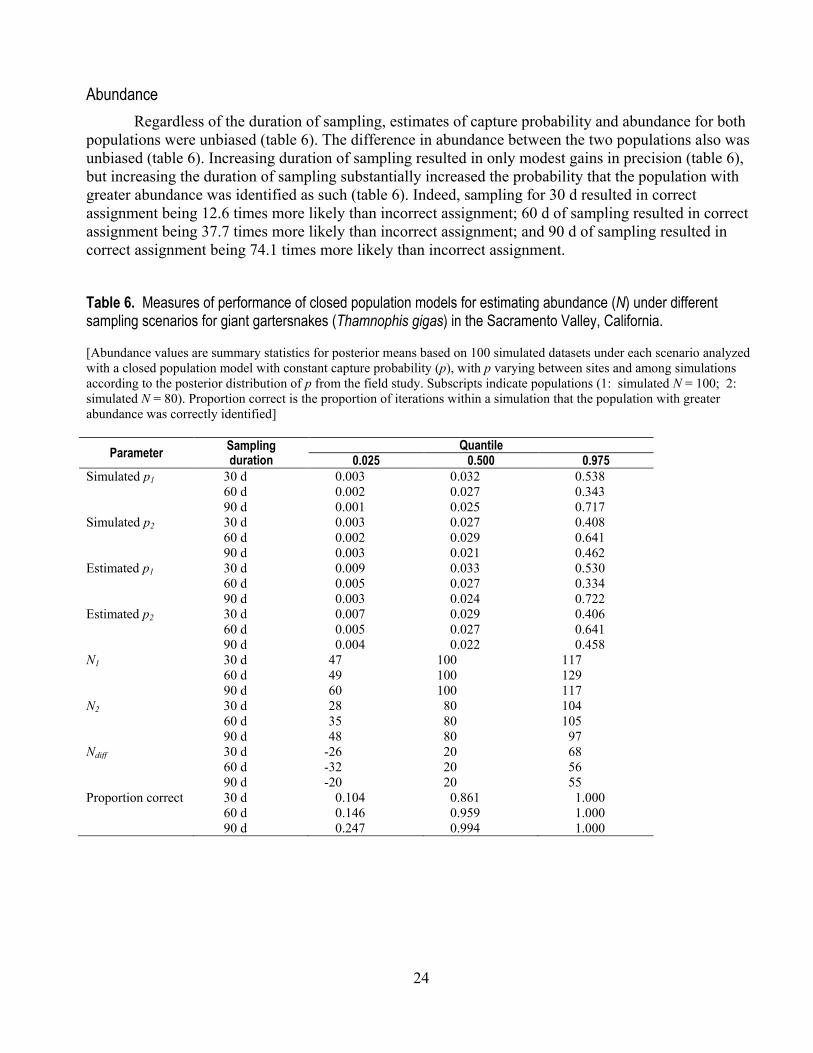
Abundance Regardless of the duration of sampling, estimates of capture probability and abundance for both

populations were unbiased (table 6). The difference in abundance between the two populations also was unbiased (table 6). Increasing duration of sampling resulted in only modest gains in precision (table 6), but increasing the duration of sampling substantially increased the probability that the population with greater abundance was identified as such (table 6). Indeed, sampling for 30 d resulted in correct assignment being 12.6 times more likely than incorrect assignment; 60 d of sampling resulted in correct assignment being 37.7 times more likely than incorrect assignment; and 90 d of sampling resulted in correct assignment being 74.1 times more likely than incorrect assignment.

Table 6. Measures of performance of closed population models for estimating abundance (N) under different sampling scenarios for giant gartersnakes (Thamnophis gigas) in the Sacramento Valley, California. [Abundance values are summary statistics for posterior means based on 100 simulated datasets under each scenario analyzed with a closed population model with constant capture probability (p), with p varying between sites and among simulations according to the posterior distribution of p from the field study. Subscripts indicate populations (1: simulated N = 100; 2: simulated N = 80). Proportion correct is the proportion of iterations within a simulation that the population with greater abundance was correctly identified]

Parameter Sampling duration

Quantile 0.025 0.500 0.975

Simulated p1 30 d 0.003 0.032 0.538 60 d 0.002 0.027 0.343 90 d 0.001 0.025 0.717 Simulated p2 30 d 0.003 0.027 0.408 60 d 0.002 0.029 0.641 90 d 0.003 0.021 0.462 Estimated p1 30 d 0.009 0.033 0.530 60 d 0.005 0.027 0.334 90 d 0.003 0.024 0.722 Estimated p2 30 d 0.007 0.029 0.406 60 d 0.005 0.027 0.641 90 d 0.004 0.022 0.458 N1 30 d 47 100 117 60 d 49 100 129 90 d 60 100 117 N2 30 d 28 80 104 60 d 35 80 105 90 d 48 80 97 Ndiff 30 d -26 20 68 60 d -32 20 56 90 d -20 20 55 Proportion correct 30 d 0.104 0.861 1.000 60 d 0.146 0.959 1.000 90 d 0.247 0.994 1.000

25

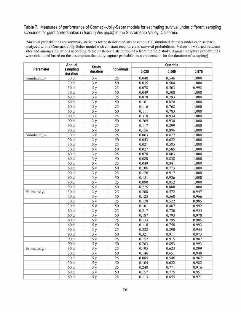
Survival Regardless of the duration of sampling, duration of study, or number of marked individuals

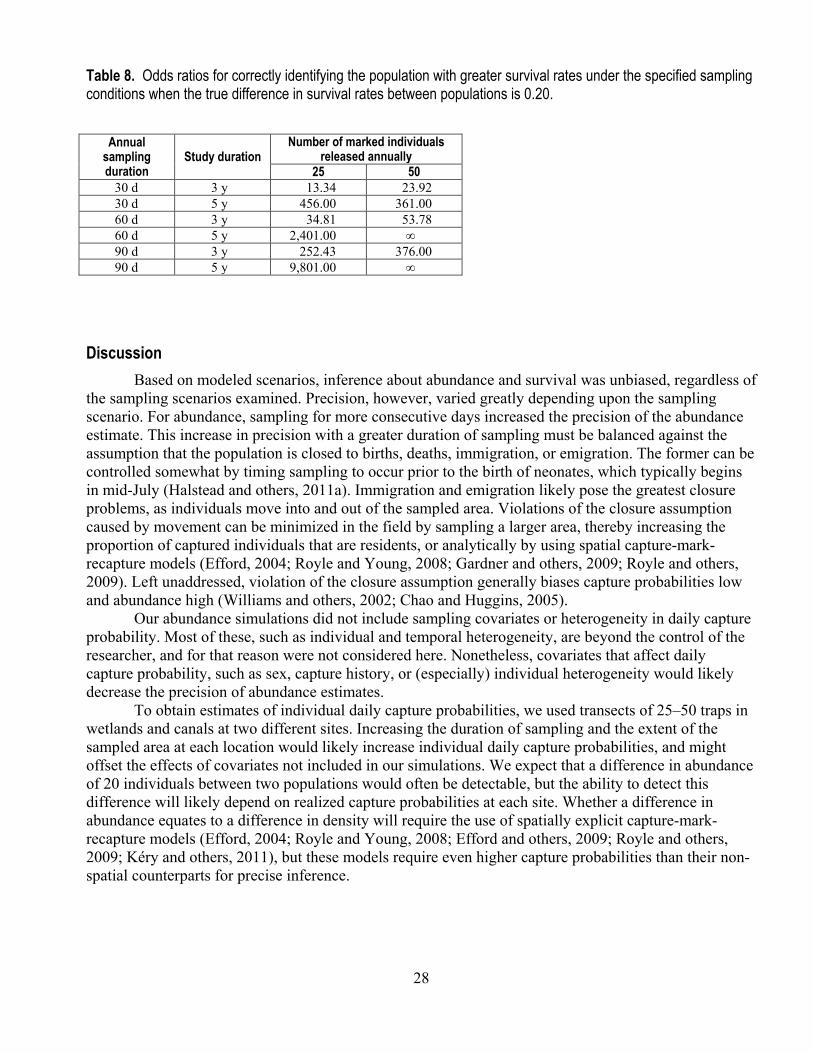
released each year, estimates of apparent survival for both populations were unbiased (table 7). The greatest gains in precision when estimating survival probability were in scenarios that increased the study duration rather than increasing the duration of sampling within a season or the number of marked individuals released each year (table 7). Under all scenarios with a sampling duration of 5 years, the odds of correctly assigning populations to higher or lower survival status were more than 360 times the odds of incorrectly assigning the populations (table 8). Odds of correct assignment were substantially reduced in studies of 3 years duration; this reduction was especially apparent when sampling duration was lower (table 8).

The mean estimated magnitude of the difference in survival probability between populations appeared to be unbiased (table 7). Study durations of 5 years resulted in more precise estimates of the difference in survival probability between the two populations (table 7). As was the case for identifying the population with higher abundance correctly, increasing the duration of sampling within a season also increased the precision of estimates of the magnitude of the difference in survival probability between the two populations, but this effect was smaller than the effect of increasing study duration (table 7).

26

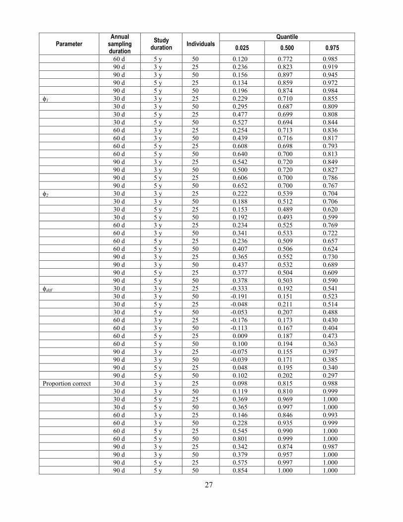
Table 7. Measures of performance of Cormack-Jolly-Seber models for estimating survival under different sampling scenarios for giant gartersnakes (Thamnophis gigas) in the Sacramento Valley, California. [Survival probabilities are summary statistics for posterior medians based on 100 simulated datasets under each scenario analyzed with a Cormack-Jolly-Seber model with constant recapture and survival probabilities. Values of p varied between sites and among simulations according to the posterior distribution of p from the field study. Annual recapture probabilities were calculated based on the assumption that daily capture probabilities were constant for the duration of sampling]

Parameter Annual

sampling duration

Study duration Individuals

Quantile 0.025 0.500 0.975

Simulated p1 30 d 3 y 25 0.040 0.546 1.000 30 d 3 y 50 0.035 0.504 1.000 30 d 5 y 25 0.078 0.503 0.998 30 d 5 y 50 0.049 0.508 1.000 60 d 3 y 25 0.078 0.793 1.000 60 d 3 y 50 0.161 0.820 1.000 60 d 5 y 25 0.116 0.768 1.000 60 d 5 y 50 0.111 0.783 1.000 90 d 3 y 25 0.318 0.934 1.000 90 d 3 y 50 0.209 0.930 1.000 90 d 5 y 25 0.117 0.899 1.000 90 d 5 y 50 0.156 0.896 1.000 Simulated p2 30 d 3 y 25 0.063 0.627 1.000 30 d 3 y 50 0.043 0.622 1.000 30 d 5 y 25 0.021 0.585 1.000 30 d 5 y 50 0.027 0.585 1.000 60 d 3 y 25 0.070 0.803 1.000 60 d 3 y 50 0.080 0.838 1.000 60 d 5 y 25 0.049 0.841 1.000 60 d 5 y 50 0.106 0.773 1.000 90 d 3 y 25 0.126 0.917 1.000 90 d 3 y 50 0.151 0.936 1.000 90 d 5 y 25 0.090 0.852 1.000 90 d 5 y 50 0.225 0.888 1.000 Estimated p1 30 d 3 y 25 0.200 0.572 0.947 30 d 3 y 50 0.125 0.560 0.966 30 d 5 y 25 0.120 0.522 0.985 30 d 5 y 50 0.101 0.487 0.992 60 d 3 y 25 0.217 0.720 0.955 60 d 3 y 50 0.187 0.793 0.970 60 d 5 y 25 0.133 0.795 0.985 60 d 5 y 50 0.118 0.758 0.993 90 d 3 y 25 0.322 0.890 0.945 90 d 3 y 50 0.321 0.911 0.973 90 d 5 y 25 0.152 0.915 0.987 90 d 5 y 50 0.203 0.893 0.993 Estimated p2 30 d 3 y 25 0.195 0.623 0.899 30 d 3 y 50 0.146 0.651 0.940 30 d 5 y 25 0.085 0.546 0.967 30 d 5 y 50 0.104 0.622 0.982 60 d 3 y 25 0.240 0.771 0.916 60 d 3 y 50 0.157 0.775 0.951 60 d 5 y 25 0.113 0.855 0.971

27

Parameter Annual

sampling duration

Study duration Individuals

Quantile 0.025 0.500 0.975

60 d 5 y 50 0.120 0.772 0.985 90 d 3 y 25 0.236 0.823 0.919 90 d 3 y 50 0.156 0.897 0.945 90 d 5 y 25 0.134 0.859 0.972 90 d 5 y 50 0.196 0.874 0.984 ϕ1 30 d 3 y 25 0.229 0.710 0.855 30 d 3 y 50 0.295 0.687 0.809 30 d 5 y 25 0.477 0.699 0.808 30 d 5 y 50 0.527 0.694 0.844 60 d 3 y 25 0.254 0.713 0.836 60 d 3 y 50 0.439 0.716 0.817 60 d 5 y 25 0.608 0.698 0.793 60 d 5 y 50 0.640 0.700 0.813 90 d 3 y 25 0.542 0.720 0.849 90 d 3 y 50 0.500 0.720 0.827 90 d 5 y 25 0.606 0.700 0.786 90 d 5 y 50 0.652 0.700 0.767 ϕ2 30 d 3 y 25 0.222 0.539 0.704 30 d 3 y 50 0.188 0.512 0.706 30 d 5 y 25 0.153 0.489 0.620 30 d 5 y 50 0.192 0.493 0.599 60 d 3 y 25 0.234 0.525 0.769 60 d 3 y 50 0.341 0.533 0.722 60 d 5 y 25 0.236 0.509 0.657 60 d 5 y 50 0.407 0.506 0.624 90 d 3 y 25 0.365 0.552 0.730 90 d 3 y 50 0.437 0.532 0.689 90 d 5 y 25 0.377 0.504 0.609 90 d 5 y 50 0.378 0.503 0.590 ϕdiff 30 d 3 y 25 -0.333 0.192 0.541 30 d 3 y 50 -0.191 0.151 0.523 30 d 5 y 25 -0.048 0.211 0.514 30 d 5 y 50 -0.053 0.207 0.488 60 d 3 y 25 -0.176 0.173 0.430 60 d 3 y 50 -0.113 0.167 0.404 60 d 5 y 25 0.009 0.187 0.473 60 d 5 y 50 0.100 0.194 0.363 90 d 3 y 25 -0.075 0.155 0.397 90 d 3 y 50 -0.039 0.171 0.385 90 d 5 y 25 0.048 0.195 0.340 90 d 5 y 50 0.102 0.202 0.297 Proportion correct 30 d 3 y 25 0.098 0.815 0.988 30 d 3 y 50 0.119 0.810 0.999 30 d 5 y 25 0.369 0.969 1.000 30 d 5 y 50 0.365 0.997 1.000 60 d 3 y 25 0.146 0.846 0.993 60 d 3 y 50 0.228 0.935 0.999 60 d 5 y 25 0.545 0.990 1.000 60 d 5 y 50 0.801 0.999 1.000 90 d 3 y 25 0.342 0.874 0.987 90 d 3 y 50 0.379 0.957 1.000 90 d 5 y 25 0.575 0.997 1.000 90 d 5 y 50 0.854 1.000 1.000

28

Table 8. Odds ratios for correctly identifying the population with greater survival rates under the specified sampling conditions when the true difference in survival rates between populations is 0.20.

Annual sampling duration

Study duration Number of marked individuals

released annually 25 50

30 d 3 y 13.34 23.92 30 d 5 y 456.00 361.00 60 d 3 y 34.81 53.78 60 d 5 y 2,401.00 ∞ 90 d 3 y 252.43 376.00 90 d 5 y 9,801.00 ∞

Discussion Based on modeled scenarios, inference about abundance and survival was unbiased, regardless of

the sampling scenarios examined. Precision, however, varied greatly depending upon the sampling scenario. For abundance, sampling for more consecutive days increased the precision of the abundance estimate. This increase in precision with a greater duration of sampling must be balanced against the assumption that the population is closed to births, deaths, immigration, or emigration. The former can be controlled somewhat by timing sampling to occur prior to the birth of neonates, which typically begins in mid-July (Halstead and others, 2011a). Immigration and emigration likely pose the greatest closure problems, as individuals move into and out of the sampled area. Violations of the closure assumption caused by movement can be minimized in the field by sampling a larger area, thereby increasing the proportion of captured individuals that are residents, or analytically by using spatial capture-mark-recapture models (Efford, 2004; Royle and Young, 2008; Gardner and others, 2009; Royle and others, 2009). Left unaddressed, violation of the closure assumption generally biases capture probabilities low and abundance high (Williams and others, 2002; Chao and Huggins, 2005).

Our abundance simulations did not include sampling covariates or heterogeneity in daily capture probability. Most of these, such as individual and temporal heterogeneity, are beyond the control of the researcher, and for that reason were not considered here. Nonetheless, covariates that affect daily capture probability, such as sex, capture history, or (especially) individual heterogeneity would likely decrease the precision of abundance estimates.

To obtain estimates of individual daily capture probabilities, we used transects of 25–50 traps in wetlands and canals at two different sites. Increasing the duration of sampling and the extent of the sampled area at each location would likely increase individual daily capture probabilities, and might offset the effects of covariates not included in our simulations. We expect that a difference in abundance of 20 individuals between two populations would often be detectable, but the ability to detect this difference will likely depend on realized capture probabilities at each site. Whether a difference in abundance equates to a difference in density will require the use of spatially explicit capture-mark-recapture models (Efford, 2004; Royle and Young, 2008; Efford and others, 2009; Royle and others, 2009; Kéry and others, 2011), but these models require even higher capture probabilities than their non-spatial counterparts for precise inference.

29

In contrast to estimating abundance, inference about survival was not substantially improved by increasing the duration of sampling within a season. Instead, increasing the duration of the study, in the present case from 3 to 5 years, greatly improved the precision of survival estimates and increased the ability to detect a difference in annual survival rates between populations. This finding is not unexpected, given that individuals recaptured over a longer time period provide more information about survival rates than individuals captured over shorter time periods. Increasing the duration of studies of survival is likely to greatly improve the precision of estimates and the reliability of inference about the populations.

As for our abundance simulations, we did not consider covariates on recapture probability or annual probability of survival. We also assumed that daily individual recapture probability was equal for all days both within and among years, and for all individuals. The presence of temporal or (especially) individual heterogeneity in recapture probability or survival probability would likely reduce the precision of estimates of survival probability. We also did not consider temporary emigration in our simulations. Temporary emigration likely occurs with giant gartersnakes, and if unaccounted for, would bias recapture probabilities low. Perhaps more important, however, temporary emigration would reduce the precision of survival estimates in studies of short duration, requiring even longer studies to generate reliable inference about survival.

Our simulations also assumed that annual survival was constant across years. If annual survival probability varies among years, then precision of survival estimates will be reduced relative to our findings. Further increasing the duration of the study is likely the most effective way to address temporal heterogeneity in survival and improve the reliability and precision of estimates of survival probability.

The finding that study duration is the most important factor tested for improving precision and inference about survival has important implications. For species like giant gartersnakes with low daily individual capture probabilities, many individuals that are alive can remain uncaptured across multiple years (similar to the temporary emigration problem above). It can therefore take many years before enough recaptures are obtained to provide precise, reliable estimates of survival probability. Based on our simulations, research that studies the application of treatments on survival of giant gartersnakes will benefit by increasing the duration of pre- and post-treatment monitoring. Observational studies of the effects of changing climatic conditions or land-use patterns will likely require even longer studies to accumulate evidence for the effects of these variables on survival. Longer monitoring than that used in our simulations will likely be required for precise inference about survival in the presence of temporary emigration or annual variation in survival.

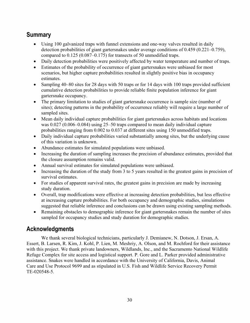
30

Summary • Using 100 galvanized traps with funnel extensions and one-way valves resulted in daily

detection probabilities of giant gartersnakes under average conditions of 0.459 (0.221–0.759), compared to 0.125 (0.087–0.175) for transects of 50 unmodified traps.

• Daily detection probabilities were positively affected by water temperature and number of traps. • Estimates of the probability of occurrence of giant gartersnakes were unbiased for most

scenarios, but higher capture probabilities resulted in slightly positive bias in occupancy estimates.

• Sampling 40–80 sites for 28 days with 50 traps or for 14 days with 100 traps provided sufficient cumulative detection probabilities to provide reliable finite population inference for giant gartersnake occupancy.

• The primary limitation to studies of giant gartersnake occurrence is sample size (number of sites); detecting patterns in the probability of occurrence reliably will require a large number of sampled sites.

• Mean daily individual capture probabilities for giant gartersnakes across habitats and locations was 0.027 (0.006–0.084) using 25‒50 traps compared to mean daily individual capture probabilities ranging from 0.002 to 0.037 at different sites using 150 unmodified traps.

• Daily individual capture probabilities varied substantially among sites, but the underlying cause of this variation is unknown.

• Abundance estimates for simulated populations were unbiased. • Increasing the duration of sampling increases the precision of abundance estimates, provided that

the closure assumption remains valid. • Annual survival estimates for simulated populations were unbiased. • Increasing the duration of the study from 3 to 5 years resulted in the greatest gains in precision of

survival estimates. • For studies of apparent survival rates, the greatest gains in precision are made by increasing

study duration. • Overall, trap modifications were effective at increasing detection probabilities, but less effective

at increasing capture probabilities. For both occupancy and demographic studies, simulations suggested that reliable inference and conclusions can be drawn using existing sampling methods.

• Remaining obstacles to demographic inference for giant gartersnakes remain the number of sites sampled for occupancy studies and study duration for demographic studies.

Acknowledgments We thank several biological technicians, particularly J. Demianew, N. Dotson, J. Ersan, A.

Essert, B. Larsen, R. Kim, J. Kohl, P. Lien, M. Meshriy, A. Olson, and M. Rochford for their assistance with this project. We thank private landowners, Wildlands, Inc., and the Sacramento National Wildlife Refuge Complex for site access and logistical support. P. Gore and L. Parker provided administrative assistance. Snakes were handled in accordance with the University of California, Davis, Animal Care and Use Protocol 9699 and as stipulated in U.S. Fish and Wildlife Service Recovery Permit TE-020548-5.

31

References Cited Amstrup, S.C., McDonald, T.L., and Manly, B.F.J., 2005, Handbook of capture-recapture analysis:

Princeton, New Jersey, Princeton University Press. California Department of Fish and Game Commission, 1971, Animals of California declared to be

endangered or threatened: California Department of Fish and Game Commission, California Code of Regulations, Title 14, Section 670.5.

Casazza, M.L., Wylie, G.D., and Gregory, C.J., 2000, A funnel trap modification for surface collection of aquatic amphibians and reptiles: Herpetological Review, v. 31, p. 91–92.

Chao, A., and Huggins, R.M., 2005, Modern closed-population capture-recapture models, in Amstrup, S.C., McDonald, T.L., and Manly, B.F.J., eds., Handbook of capture-recapture analysis: Princeton, New Jersey, Princeton University Press, p. 58–87.

Coates, P.S., Wylie, G.D., Halstead, B.J., and Casazza, M.L., 2009, Using time-dependent models to investigate body condition and growth rate of the giant gartersnake: Journal of Zoology, v. 279, p. 285–293.

Efford, M.G., 2004, Density estimation in live-trapping studies: Oikos v. 106, p. 598–610. Efford, M.G., Dawson, D.K., and Borchers, D.L., 2009, Population density estimated from locations of

individuals on a passive detector array: Ecology, v. 90, p. 2,676–2,682. Fitch, H.S., 1940, A biogeographical study of the ordinoides artenkreis of garter snakes (genus

Thamnophis): University of California Publications in Zoology, v. 44, p. 1–150. Frayer, W.E., Peters, D.D., and Pywell, H.R., 1989, Wetlands of the California Central Valley—Status

and trends, 1939–mid-1980s: U.S. Fish and Wildlife Service, Region 1, Portland, Oregon. Gardner, B., Royle, J.A., and Wegan, M.T., 2009, Hierarchical models for estimating density from DNA

mark-recapture studies: Ecology, v. 90, p. 1,106–1,115. Gelman, A., and Rubin, D.B., 1992, Inference from iterative simulation using multiple sequences:

Statistical Science, v. 7, p. 457–472. Halstead, B.J., Skalos, S.M., Casazza, M.L., and Wylie, G.D., 2015, A preliminary investigation of the

variables affecting the distribution of giant gartersnakes (Thamnophis gigas) in the Sacramento Valley, California: U.S. Geological Survey Open-File Report 2015-1178, 34 p.

Halstead, B.J., Wylie, G.D., and Casazza, M.L., 2010, Habitat suitability and conservation of the giant gartersnake (Thamnophis gigas) in the Sacramento Valley of California: Copeia, v. 2010, p. 591–599.

Halstead, B.J., Wylie, G.D., and Casazza, M.L., 2013, Efficacy of trap modifications for increasing capture rates of aquatic snakes in floating aquatic funnel traps: Herpetological Conservation and Biology, v. 8, p. 65–74.

Halstead, B.J., Wylie, G.D., Casazza, M.L., and Coates, P.S., 2011a, Temporal and maternal effects on reproductive ecology of the giant gartersnake (Thamnophis gigas): The Southwestern Naturalist, v. 56, p. 29–34.

Halstead, B.J., Wylie, G.D., and Casazza, M.L., 2014, Ghost of habitat past: historic habitat affects the contemporary distribution of giant garter snakes in a modified landscape: Animal Conservation, v. 17, p. 144‒153.

Halstead, B.J., Wylie, G.D., Coates, P.S., and Casazza, M.L., 2011b, Bayesian adaptive survey protocols for resource management: Journal of Wildlife Management, v. 75, p. 450–457.

Halstead, B.J., Wylie, G.D., Coates, P.S., Valcarcel, P., and Casazza, M.L., 2012, Bayesian shared frailty models for regional inference about wildlife survival: Animal Conservation, v. 15, p. 117–124.

32

Hansen, G.E., and Brode, J.M., 1980, Status of the giant garter snake Thamnophis couchii gigas (Fitch):

Sacramento, California Department of Fish and Game, Inland Fisheries Endangered Species Program Special Publication Report Number 80-5, 14 p.

Hansen, R.W., and Hansen, G.E., 1990, Thamnophis gigas (giant garter snake) reproduction: Herpetological Review, v. 21, p. 93–94.

Kéry, M., 2002, Inferring the absence of a species—A case study of snakes: Journal of Wildlife Management, v. 66, p. 330–338.

Kéry, M., 2010, Introduction to WinBUGS for ecologists—A Bayesian approach to regression, ANOVA, mixed models and related analyses: Burlington, Massachusetts, Academic Press.

Kéry, M., Gardner, B., Stoeckle, T., Weber, D., and Royle, J.A., 2011, Use of spatial capture-recapture modeling and DNA data to estimate densities of elusive animals: Conservation Biology, v. 25, p. 356–364.

Kéry, M., and Schaub, M., 2011, Bayesian population analysis using WinBUGS—A hierarchical perspective: Waltham, Massachusetts, Academic Press.

Kuo, L., and Mallick, B., 1998, Variable selection for regression models: Indian Journal of Statistics, v. 60, p. 65–81.

MacKenzie, D.I., Nichols, J.D., Lachman, G.B., Droege, S., Royle, J.A., and Langtimm, C.A., 2002, Estimating site occupancy rates when detection probabilities are less than one: Ecology, v. 83, p. 2,248–2,255.

MacKenzie, D.I., Nichols, J.D., Royle, J.A., Pollock, K.H., Bailey, L.L., and Hines, J.E., 2006, Occupancy estimation and modeling—Inferring patterns and dynamics of species occurrence: Amsterdam, The Netherlands, Academic Press.

MacKenzie, D.I., and Royle, J.A., 2005, Designing occupancy studies—General advice and allocating survey effort: Journal of Applied Ecology, v. 42, p. 1,105–1,114.

Mazerolle, M.J., Bailey, L.L., Kendall, W.L., Royle, J.A., Converse, S.J., and Nichols, J.D., 2007, Making great leaps forward—Accounting for detectability in herpetological field studies: Journal of Herpetology, v. 41, p. 672–689.

Plummer, M., 2014a, JAGS—A program for analysis of Bayesian graphical models using Gibbs sampling, Version 3.4.0, in Hornik, Kurt, Leish, Friedrich, and Zeileis, Achim, Proceedings of the 3rd International Workshop on Distributed Statistical Computing: Workshop on Distributed Statistical Computing 2003 Working Papers, 10 p.

Plummer, M., 2014b, rjags—Bayesian graphical models using MCMC: JAGS, R package version 3-14. R Core Team, 2014, R—A language and environment for statistical computing: Vienna, Austria, R

Foundation for Statistical Computing. Rossman, D.A., Ford, N.B., and Seigel, R.A., 1996, The garter snakes—Evolution and ecology:

Norman, Oklahoma, University of Oklahoma Press. Rossman, D.A., and Stewart, G.R., 1987, Taxonomic reevaluation of Thamnophis couchii (Serpentes:

colubridae): Occasional Papers of the Museum of Zoology, Louisiana State University, v. 63, p. 1–25. Royle, J.A., and Dorazio, R.M., 2008, Hierarchical modeling and inference in ecology—The analysis of

data from populations, metapopulations and communities: London, Academic Press. Royle, J.A., Karanth, K.U., Gopalaswamy, A.M., and Kumar, N.S., 2009, Bayesian inference in camera

trapping studies for a class of spatial capture–recapture models: Ecology, v. 90, p. 3,233–3,244. Royle, J.A., and Young, K.V., 2008, A hierarchical model for spatial capture-recapture data: Ecology, v.

89, p. 2,281–2,289.

33

U.S. Fish and Wildlife Service, 1993, Endangered and threatened wildlife and plants—Determination of

threatened status for the giant garter snake: Federal Register, v. 58, p. 54,053–54,066. U.S. Fish and Wildlife Service, 1999, Draft recovery plan for the giant garter snake (Thamnophis gigas):

U.S. Fish and Wildlife Service, 192 p. Williams, B.K., Nichols, J.D., and Conroy, M.J., 2002, Analysis and management of animal

populations: San Diego, California, Academic Press. Winne, C.T., Willson, J.D., Andrews, K.M., and Reed, R.N., 2006, Efficacy of marking snakes with

disposable medical cautery units: Herpetological Review, v. 37, p. 52–54. Wylie, G.D., Casazza, M.L., Gregory, C.J., and Halstead, B.J., 2010, Abundance and sexual size

dimorphism of the Giant Gartersnake (Thamnophis gigas) in the Sacramento Valley of California: Journal of Herpetology, v. 44, p. 94–103.

Wylie, G.D., Casazza, M.L., Halstead, B.J., and Gregory, C.J., 2009, Sex, season, and time of day interact to affect body temperatures of the Giant Gartersnake: Journal of Thermal Biology, v. 34, p. 183–189.

34

Glossary

Abundance: The number of individuals of a population in the sampled area. Algorithm: A set of rules for solving a problem in a finite number of steps. Allopatric: Occupying different geographical areas. Bayesian analysis: A method of statistical inference in which Bayes’ rule is used to update probability distributions as data are acquired. Bias: Systematic (as opposed to random) distortion of a statistic as the result of a sampling or analytical procedure. Brumation: A state of dormancy in reptiles and amphibians similar to hibernation, but involving different metabolic processes. Capture-mark-recapture: A method of estimating demographic parameters of populations for which individuals cannot be directly counted that involves capturing, marking, and recapturing individuals. Not all capture-mark-recapture methods require physical capture of individuals (for example, camera traps, hair snares for DNA, etc.). Capture history: A sequence of (usually) 0s and 1s indicating sampling occasions on which an individual was (1) or was not (0) observed. Capture probability: The per-survey probability that a specific individual is captured or observed. Centrarchidae: A family of freshwater ray-finned fishes in the order Perciformes that includes the sunfish (for example, largemouth bass, bluegill, pumpkinseed, and crappie). Closed model: A capture-mark-recapture model that assumes that the population does not change (that is, is closed to births, deaths, immigration, and emigration) for the duration of sampling. Coefficient: A parameter of a statistical (regression) model that indicates how the response variable changes with the predictor variable; analogous to the slope of a line. Cormack-Jolly-Seber model: An open population model that estimates apparent survival by conditioning on the first capture of individuals. Confidence interval: A statistical interval estimate of a parameter such that, if constructed across many replicated experiments, the proportion of such intervals that contain the true fixed value of the parameter equals the given confidence level. Convergence: The meeting and overlapping of independent Markov chains in a Markov-chain Monte Carlo simulation, used to assess whether the stationary posterior distribution has been reached. Covariate: A (predictor) variable thought to be correlated with another (response) variable used in a regression analysis. Credible interval: A specified domain of the posterior probability distribution used for interval estimation. Credible intervals can be interpreted as the probability, confidence, or belief that a parameter or value falls within the specified region. Cumulative detection probability: The probability of detecting an individual or species across multiple surveys. Calculated as 1 −∏ �1 − 𝑝𝑗�𝑛

𝑗=1 , where pj is the per-survey detection or capture probability and n is the total number of surveys. Cyprinidae: A large family of freshwater fishes containing the carps, minnows, and their relatives.

35

Data augmentation: The addition of data to assist in the solving of a problem. In capture-mark-recapture applications, it is the addition of individuals that were not observed to those that were observed to estimate how many of the unobserved individuals were part of the population. Demography: The scientific study of populations, especially with regard to their size, structure, distribution, and dynamics. Density: The number of individuals in a population per unit area or volume. Detection history: A sequence of (usually) 0s and 1s indicating sampling occasions on which at least one individual was (1) or was not (0) observed at a sampled site. Detection probability: In occupancy modeling, the per-survey probability that any individual of a species is observed. Dimorphic: Having two forms. Extirpate: To cause a species to go extinct within a portion of its range. Finite population inference: Inference made to a finite number of samples under consideration, rather than to the infinite number of possible samples often assumed in statistical theory. Forage: To search for food. Full model: The model containing the entire set of predictors (and their potential interactions) considered. Gravid: Pregnant. Heterogeneity: Differences among units within a group. Indicator variable: A variable taking a value of 1 if the corresponding condition is included in a model, or a value of 0 if the corresponding condition is not included in a model. Litter: The number of young brought forth by an iteroparous animal at one parturition. Markov-chain Monte Carlo (MCMC): A class of algorithms for sampling from a probability distribution based on constructing a Markov chain that has the desired distribution as its equilibrium distribution. Metabolic: Of, relating to, or affected by metabolism. Morphology: The form and structure of an organism. Natricinae: A subfamily of the family Colubridae of snakes, which includes European grass snakes and North American watersnakes and gartersnakes. Neonate: A newborn. Obligate: Restricted to a particular condition. Occupancy: The condition of a site, habitat, etc. being occupied by a species. Occurrence: The state of a site, habitat, etc. being occupied by a species. Parturition: The act or process of giving birth to offspring. Posterior distribution: The probability distribution of an unknown quantity conditional on the evidence obtained from an experiment or survey, possibly taking into account relevant information available prior to the experiment or survey. Posterior probability: The conditional probability assigned to a random event after relevant evidence or background as been taken into account. Precinctive: Restricted to a defined geographic area. Prior probability: The probability distribution that expresses one’s uncertainty about an unknown quantity before some evidence (experiment, survey, observation, etc.) is taken into account. Pseudo-individual: An unobserved individual that might or might not be part of a population and is given an all-zero capture history during data augmentation for analysis of capture-mark-recapture models.

36

Quadratic: Involving the square of a predictor variable in a regression model. Range: The geographic limits within which all individuals of a species are found, excluding those in captivity. Species: The basic category of biological classification, ranking below a genus and consisting of related individuals capable of interbreeding. Subspecies: A subdivision of a species, especially a geographical or ecological subdivision. Subterranean: Existing, situated, or operating below the surface of the earth; underground. Static occupancy model: A model that describes the proportion of sites or area occupied by a species at a specific point in time (that is, assuming that sites or sample units are not colonized or extirpated during the sampling period), explicitly accounting for imperfect detection of species. Survival: The rate or probability at which individuals alive at time t remain alive until time t + 1. Sympatric: Occupying the same geographical area. Taxonomy: The branch of biology dealing with the description, identification, naming, and classification of organisms. Temporary emigration: The temporary movement of individuals outside the sampled area. Transect: A line used in ecological surveys to measure and characterize plant or animal distributions or populations within a given area. Unbiased: Having an expected value equal to the parameter being estimated. Uninformative prior: A prior probability distribution that expresses vague or general information about a variable, typically with the goal of assigning equal probabilities to all possibilities.

Publishing support provided by the U.S. Geological SurveyScience Publishing Network, Tacoma Publishing Service Center

For more information concerning the research in this report, contact the Director, Western Ecological Research Center

U.S. Geological Survey 3020 State University Drive East Sacramento, California 95819 http://www.werc.usgs.gov/

http://www.werc.usgs.gov/

Halstead and others—D

etection and Capture Probabilities for Giant Gartersnakes U

sing Floating Aquatic Funnel Traps—

Open–File Report 2015–1200

ISSN 2331-1258 (online)http://dx.doi.org/10.3133/ofr20151200

Documents

Realized Detection and Capture Probabilities for Giant - · PDF fileOpen-File Report 2015–1200. ... Realized Detection and Capture Probabilities for Giant Gartersnakes (Thamnophis