Economic Research Southern Africa (ERSA) is a research programme funded by the National

Treasury of South Africa. The views expressed are those of the author(s) and do not necessarily represent those of the funder, ERSA or the author’s affiliated

institution(s). ERSA shall not be liable to any person for inaccurate information or opinions contained herein.

Realized correlations, betas and volatility

spillover in the commodity market: What

has changed?

Matteo Bonato

ERSA working paper 639

October 2016

Realized correlations, betas and volatility spillover in thecommodity market: What has changed?

Matteo Bonato∗

University of Johannesburg

Current Draft: September 2016

Abstract

This papers adopts the recently proposed realized Beta GARCH model of Hansen et al. (J.Appl. Econ. (2014)) to examine the changes in price and return dynamics that affected the com-modity market during the 2007-2008 boom and bust. We provide evidence that, starting from2006, realized correlations between agricultural commodities within the same group significantlyincreased. Moreover, the observed increase in correlations between agriculturals and oil wasgreater still. The dynamics of the volatility spillover across commodities are also investigated. It isfound that spillover effects became more evident prior to the commodity price crash. However, thisincrease in volatility transmission tended to anticipate the increase in correlations. To conclude,it is shown that the size of a short position in oil required to hedge a long agricultural commodityposition , given by the realized beta, therefore increased significantly.

Keywords: Commodities; Correlation; Beta; Volatility Spillover; Realized Measures

1 Introduction

In the recent years, the availability of different type of commodity futures indices has made investing inthe commodity market widely accessible to new players seeking a capital allocation which offered di-versification with respect to the equity, currency and fixed income markets and which is also positivelycorrelated with changes inflation (Schofield, 2007).

As a consequence, commodity futures have emerged, starting from early 2000, as popular assetclass as investors turned to commodities as a means to diversify their portfolios (Cheng and Xiong,2014). The large fluctuations in commodity prices observed amid the latest financial crisis and thecrash which occurred in late 2008 have contributed to attract a considerable level of academic atten-tion. A set of stylized empirical facts characterizing the commodity prices has emerged, see Chengand Xiong (2014) for a comprehensive review.

First, a proper commodity ‘super-cycle’ has been experienced in the last 10 years with the result-ing boom and bust of futures prices. This had as a consequence an extreme increase in commodityreturns volatility, which is more pronounced for index commodities than for off-index commodities.

Secondly, an increase in cross-commodity correlations has also been observed. As evidencessuggest before the early 2000s, commodity market were partially segmented from outside financial

∗Address: Department of Economics and Econometrics, University of Johannesburg. E-mail: mbonato@uj.ac.za. Partof this paper was written while I was visiting the Department of Economics at the University of Pretoria and the Departmentof Statistics at the University of Zimbabwe in Harare. Their hospitality is gratefully acknowledged. Part of this research wassupported by the Economic Research Southern Africa (ERSA). I would like to thank Peter Reinar Hansen and Asger Lundefor sharing their Matlab codes; Duc Khuong Nguyen and Luca Taschini for their useful suggestions. All remaining errorsare mine.

1

markets and from each others. Erb and Harvey (2006) showed that commodities had only low pos-itive return correlations with each other. Gorton and Rouwenhorst (2006) did not find evidences ofcorrelations between commodity returns and the S&P 500 returns, especially at short horizons (dailyand monthly). This segmentation does no longer hold. The correlations of different sectors of theGoldman Sach Commody Index (GSCI) with the GSCI Energy index rose from a pre-2004 rangebetween ± 20% to reach 70% in 2008. This phenomenon is observed also within the same sector.Furthermore, the correlation of commodity returns with returns on other asset classes has also in-creased, e.g. increasing correlations between GSCI Total Return Index and MSCI Emerging MarketIndex, DXY US Dollar Index 1, 10-year US Treasury yield and CRSP Value-weighted Index.

Last, along with increasing volatility and correlation, volatility spillover effects have been foundbetween commodities and between commodities and other assets.

In this paper we present a novel set of analyses whose goal is to provide further evidences of thechanges in price and return dynamics in the commodity market around the 2007-2008 boom&bust.We focus our attention on three main statistics which describe the linkage between commodities:correlations, volatility spillovers and optimal hedging ratios (or betas).

Asset correlation dynamics are crucial in portfolio management and risk hedging as investorsseek to diversify their allocations by targeting lowly correlated assets. Our results show that startingfrom 2005, correlations between commodities started to significantly increase, therefore wiping outthe diversification benefit for which commodities were chosen in first place. This feature, first noted inTang and Xiong (2012), is also confirmed in a recent paper by Dorman and Karali (2014). Examiningcommodity data from 1990 through 2011 they find that simple correlation coefficients between futuresprices and the probability of nonstationarity of the series have increased over time, therefore signalingthat the commodity market is shown to become more efficient after 2004.

Along with correlations, spillovers effect are also an important aspect to be considered when deal-ing with a portfolio of assets. Indeed, a surge in assets volatility, together with an increase in volatilitytransmission, affects optimal portfolio allocations and can result in greater costs for managing risks(e.g. higher hedging costs). It is therefore crucial to understand and possibly anticipate changes involatility relationships in order to develop appropriate risk management strategies. Volatility spillovershave been studied abundantly in the financial literature. See for example Baele (2005), Bekaertand Harvey (1997), Bekaert et al. (2002), Christiansen (2007), Ng (2000). For applications on high-frequency data see Bonato et al. (2013) and Fengler and Gisler (2014). While these works all focuson the equity, currencies or bond markets, only recently has the academic literature started to inves-tigate this topic in the commodity market, and especially between oil and agricultural commodities oroil and the stock market; see the seminal paper of Wu et al. (2010) and Chang et al. (2013), Arouriet al. (2011), Mensi et al. (2013) also amongst others.

We conclude the empirical analyses by showing how hedging strategies have also been affectedby the latest development of the commodity market dynamics. Particular attention will be given to theinteraction between oil and agricultural commodities.

Within our analyses we focus in particular on the interaction between oil and agricultural com-modities. In the academic literature, particular attention has been given the the interaction betweenenergy commodities (specifically oil) and agricultural commodities. The rise of energy prices alongwith the boom in agricultural commodity prices - which led to the so called ‘food crisis’ - raised thequestion of whether energy markets have any explanatory power on the observed upward movementin agricultural food prices. The political implications of such nexus would indeed very important.

Different hypothesis to link oil and agricultural prices have been suggested. First, the relationbetween oil and agricultural prices is motivated by oil being a production cost. Baffes (2007) analyzedhow crude oil prices spill on the price of 35 internationally traded primary commodities and found that

1Multiplied by -1

2

the pass-through of crude oil shocks to the overall non-energy commodity index, the fertilizer index,agriculture and metals are 0.16, 0.33, 0.17, respectively.

The positive comovement between oil and agricultural commodities can be also motivated usingthe substitutive effect between biofuels and fossil fuel. An increase in oil prices inspire people todevelop alternative sources of energy: the bioethanol and biodiesl extracted from corn and soybean,respectively, are considered the appropriate substitute of crude oil. Thus, increase in oil prices canresult in the increase of corn and soybean prices and finally lead to the surge in prices of the otheragricultural commodities as the planting acreage is limited in a certain period of time (Chang and Su,2010). In terms of volatility spillover, Wu et al. (2010) show that spillover intensities from crude oilprices onto corn prices (spot and futures) have increased significantly since the Energy Policy Act of2005. This act established the Renewable Fuel standard requiring that transportation fuels sold in theUnited States contain a minimum amount of renewable flues. Subsequent tax incentives, federal andstate mandates and the progressive elimination of Methyl Tertiary Butyl Ether as an additive in manystates have quickly increased the demand for biofuels, particularly corn-based ethanol.

A third hypothesis argues that global economic activity, rather than increases in oil prices, is themain driver of higher agricultural commodity prices, see Krugman (2008), Hamilton (2009), Kilian(2009). The development of emerging economies (China and India in particular) in the past decadehas stimulated unprecedented demands for a broad range of commodities in sectors like energy andmetal. This may have led to a joint price boom for commodities.

A last explanation presented by Tang and Xiong (2012), which is alternative to both the biofueland global economic activity hypothesis, links the increase correlation between oil and non-energycommodity prices to the financialization of the commodity market. The authors argue that, as a resultof the financialization process, the price of an individual commodity is no longer determined solelyby its demand and supply. Instead, prices are also determined by the aggregate risk appetite forfinancial assets and the investment behavior of diversified commodity index investors.

From the methodological side we rely in the realized beta GARCH model of Hansen et al. (2014).The realized beta GARCH is a multivariate volatility model which incorporates both generalized au-toregressive conditional heteroskedasticity (GARCH) and realized measures of variances and co-variances. Realized measures are important as they extract information about the current levels ofvolatilities and correlations from high-frequency data. This is particularly useful for modeling financialreturns during periods of rapid changes in the underlying covariance structure. The model has a hi-erarchical structure: the ‘market’ return is modeled with a univariate realized GARCH model (Hansenand Huang, 2012; Hansen et al., 2012)). In principle, other approaches based on multivariate GARCH(DCC, BEKK) could be employed in order to estimate dynamic correlations and assess the spillovereffects. We decided instead to adapt the realized beta GARCH to the commodity case. On the onehand, this enables us to consider the price and return information available at intra-day frequency.On the other hand the mode lends itself well to represent fit the commodity market composition. Inthe realized beta GARCH model the multivariate structure is constructed by modeling ‘individual’ re-turns conditional on the past and contemporary market variables (return and volatility). This makesit feasible to extract the ’betas’ but also account for contemporaneous volatility spillover between themarket and the single asset. In our setup, for each agricultural commodity class (Grains and Softs),we impose the most material single-name commodity to be the market variable. This enables us tomeasure the changes in correlations within a same class. Then, following the approach of Tang andXiong (2012), we make use of oil as the market variable thus allowing to assess how correlationsbetween Agriculturals and oil developed.

Our work contributes to the literature studying the interaction between oil and agricultural com-modities by presenting an innovative approach based on a recently introduced multivariate model forrealized measures. This model combines the information contained in the high frequency intra-dayprice observations with a conditional heteroskedasticity model. It also possess a hierarchical structure

3

in which each single commodity return is modeled as function of the ‘market’ return, in a CAPM-likefashion. This setup adapts itself very well to our purposes as we use one commodity (the mostrepresented in the commodity indices) as proxy for the market and extrapolate the model realizedcorrelation between this commodity and each single commodities along with the (contemporaneous)spillover effect.

Our results confirm that agricultural commodities belonging to the same sector (Softs or Grains)experience an increase in correlations staring from 2006. Correlations between oil and those com-modities has also significantly increased. Additionally, we find that, along with increased correlations,spillover effects of oil on agricultural commodities became more prominent, especially around theraise and fall of the commodity market. To conclude, we show how these changes affected the op-timal hedging ratios, defined in term of realized betas. The optimal hedging ratio is the amount ofdollars to be invested in a short position in an asset in order to hedge a 1$ long position in an otherasset. In our setting, the representative investor is assumed to hedge a long position in an agricul-tural future with a short position in oil. Our results show a marked increase in optimal hedging ratios.A consequence of this is that hedging costs have also increased. This is coherent with our previ-ous findings since an increase in correlations results in lower diversification benefits and increase inspillover effect induces higher volatility risk. This obviously drives the cost of protecting against riskhigher.

The paper is structured as follows: Section 2 introduces the econometric approach adopted,i.e. the realized Beta modes of Hansen et al. (2014) and its adaptation the the case of commodities;Section 3 presents the dataset used; empirical results are reported in Section 4: realized correlations,spillover effects and optimal hedging ratios; Section 5 concludes.

2 Econometric methodology

2.1 Realized Beta GARCH

The realized beta GARCH proposed by Hansen et al. (2014) is a multivariate volatility model whichincorporates both generalized autoregressive conditional heteroskedasticity (GARCH) and realizedmeasures of variances and covariances. Realized measures are important as they extract informationabout the current levels of volatilities and correlations from high-frequency data. This is particularlyuseful for modeling financial returns during periods of rapid changes in the underlying covariancestructure. The model has a hierarchical structure: the ‘market’ return is modeled with a univariaterealized GARCH model (Hansen and Huang, 2012; Hansen et al., 2012)). A multivariate structureis constructed by modeling ‘individual’ returns conditional on the past and contemporary market vari-ables (return and volatility). The resulting model has the structure of a dynamic capital asset pricingmodel (CAPM) that makes it feasible to extract the ’betas’ but also account for contemporaneousvolatility spillover between the market and the single asset.

Let r0,t and x0,t denote the market return and a corresponding realized measure of volatility,respectively. Similarly, the notation r1,t and x1,t denote the same variable associated with an individ-ual asset returns. Realized measures of volatility are constructing using the information available atintra-day frequency. This approach was pioneered by Andersen and Bollerslev (1998). The classicalestimator of the realized volatility reads

x0,t =

I∑i=1

r20,t−1+ih,h (1)

where r0,t−1+ih,h ≡ p0,t−1+ih−p0,t−1+(i−1)/h denotes the vector of returns for the i-th intraday periodon day t, for i = 1, . . . , I. I refers to the number of intraday intervals, each of length h ≡ 1/I. Under

4

the assumption that the process is continuous and no market microstructure noise is present, thisestimator provides an accurate measures of the process integrated variance.

Define the conditional variance h0,t = var(r0,t|Ft−1) and h1,t = var(r1,t|Ft−1). Define also theconditional correlation ρ1,t = corr(r0,t, r1,t|Ft−1); it follows directly that the realized version of the‘beta’

β1,t = cov(r1,t, r0,z|Ft−1)/var(r0,t|Ft−1) (2)

is given by

β1,t = ρ1,t

√h1,th0,t

. (3)

The model for the market return and realized measures of volatility takes the form of an exponen-tial GARCH. It is described by the following three equations

ro,t = µ0 +√h0,tz0,t (4)

log h0,t = a0 + b0 log h0,t−1 + c0 log x0,t−1 + τ0(z0,t−1) (5)

log x0,t = ξ0 + φ0 log h0,t + δ0(z0,t) + u0,t, (6)

where zo,ti.i.d.∼ N(0, 1) and uo,t

i.i.d.∼ N(0, σ2u,0). The functions τ(z) and δ(z) are called leveragefunctions because they model aspects related to the leverage effects, which refers to the dependencebetween returns and volatility. They are defined as τ(z) = t1z+t2(z

2−1) and δ(z) = δ1z+δ2(z2−1).

Equations (5) and (6) are referred to as the return equation and the GARCH equation, respectively.The third equation, ((6)), is called the measurement equation and completes the specification of thedensity f(r0,t, x0,t|Ft−1).

To conclude, a model for the time series associated with the individual asset needs to be formu-lated, conditional on the contemporaneous ‘market’ variables. This reads

r1,t = µ1 +√h1,tz1,t (7)

where the dependence on (r0,t, x0,t) operates through ρ1,t = cov(z0,1, z1,t|Ft−1), the conditionalcorrelation. The factor structure is then revealed:

z1,t = ρ1,tz0,t +√

1− ρ21,tω1,t (8)

where ω1,t = (z1,t − ρ1,tz0,t)/√

1− ρ31,t has mean zero, unit variance and it is uncorrelated withz0,t. This implies that the studentized returns for the individual asset is a linear combination of thestudentized market return and the idiosyncratic component ω1,t, where the relative weight, defined byρ1,t is time varying. The model concludes by specifying the dynamics for h1,t and ρ1,t. For h1,t theGARCH equation is used

log h1,t = a1 + b1 log h1,t−1 + c1 log x1,t−1 + d1 log h0,t + τ1(z1,t−1). (9)

The parameter d1 can be interpreted as contemporaneous spillover effect, measuring the extent towhich the market’s volatility affects the volatility of the individual asset while accounting for the asset-specific volatility dynamics. The model is formulated in a way that h0,t is Ft−1-measurable, so thepresence of h0,t on the right-hand side of the equation does not contradict the definition of h1,t.

For the dynamics of ρ1,t a Fisher transformation is adopted, ρ → F (ρ) = 12 log 1+ρ

1−ρ which is aone-to-one mapping from (-1, 1) into R. The GARCH equation for the transformed correlation is givenby

F (ρ1,t) = a10 + b10F (ρ1,t−1) + c10F (y1,t−1).

5

Finally, the following measurement equations specify the conditional densities for the two realizedmeasures

log x1,t = ξ1 + ψ1 log h1,t + δ1(z1,t) + u1,t (10)

F (y1,t) = ξ10 + ψ10F (ρ1,t) + ν1,t. (11)

The model is estimated via maximum likelihood. The marginal model for the market variablesclosely follow that of Hansen et al. (2012) and can be further decomposed into the conditional den-sities of r0,t and of x0,t|r0,t. The likelihood contribution for the conditional model for individual assetsalso permits a further decomposition into the conditional densities of r1|r0,x0 and (x1, y2|r1, r0, x0).

2.2 Market model for commodities

The realized beta GARCH model described above lends itself well not only to situations in which oneis interesting in a dynamic CAPM framework, but it provides a very flexible tool to asses the dynamicsof the correlations, spillovers effects and optimal hedge ratios between two individual assets belongingto the same class.

In this paper we focus in particular on the commodity market. Our goal is to investigate the behav-ior of correlations, changes in spillover effects and optimal hedge ratios within agricultural commodi-ties and between oil and agricultural commodities as effect of the recent boom & bust (also referredby some as ‘food crisis’, see Wang et al., 2014) the commodity market experienced in starting from2005.

We use two major commodities, corn and sugar, as representative of the market commodity forthe Grains and Softs sector, respectively. We chose corn and sugar as they are the commodities withthe largest weight per sector in the three major commodity indices in Table 1. In a next step, we useoil as proxy for the commodity market index in order to describe the commodity market as a whole.The choice of oil as commodity market index proxy follows Tang and Xiong (2012) and is motivatedby the fact that oil is the commodity receiving the largest weights in two important commodity indices:S&P Goldman Sachs and the Dow Jones UBS.

As a consequence of the financialization of the commodity market, Tang and Xiong (2012) showhow prices of non-energy commodity futures in the United States have become increasingly corre-lated with oil prices. Following the lines of Barberis et al. (2005), Bonato and Taschini (2015) confirmthat this increase in comovement across commodities and with oil cannot be explained as only drivenby fundamentals and provide new evidences supporting the friction or sentiment based view expla-nations.

3 Data

A total of 28 commodity futures are traded in the US market. Table 1 considers, out of these 28, 4Grain commodities (corn, soy beans, chicago wheat and soybean oil), 4 Soft commodities (coffee,cotton, cugar and cocoa) and oil. For each of this commodity we also report the weight associatedwith three major commodity indices: S&P GSCI, UBS-DJ CI and Thomson-Reuters CI.

Data are provided by disktrading.com and are at 1-minute frequency covering the trading hourof the CME and ICE. Globex trading information (i.e. outside the markets trading hours) is at ourdisposal for major commodities only and is therefore not used. Futures data are in continuous formatcontaining price data of the most actively traded contracts. Close to expiration of a contract, theposition is rolled over to the next available contract, provided that activity has increased. In orderto guarantee that our results are based on overlapping time periods, we only considered trades thatoccurred between 10.30 and 14.00. Our data set spans the period going from Jan 2, 2002 to March

6

24, 2011, for a total of 2,281 trading days. Daily prices of the commodities under analyses are plottedin Figure 1

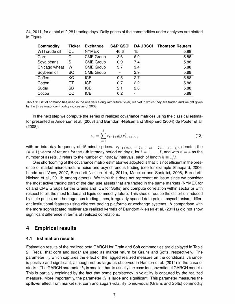
Commodity Ticker Exchange S&P GSCI DJ-UBSCI Thomson ReutersWTI crude oil CL NYMEX 40.6 15 5.88Corn C CME Group 3.6 6.9 5.88Soya beans S CME Group 0.9 7.4 5.88Chicago wheat W CME Group 3.7 3.4 5.88Soybean oil BO CME Group - 2.9 5.88Coffee KC ICE 0.5 2.7 5.88Cotton CT ICE 0.7 2.2 5.88Sugar SB ICE 2.1 2.8 5.88Cocoa CC ICE 0.2 - 5.88

Table 1: List of commodities used in the analysis along with future ticker, market in which they are traded and weight givenby the three major commodity indices as of 2008.

In the next step we compute the series of realized covariance matrices using the classical estima-tor presented in Andersen et al. (2003) and Barndorff-Nielsen and Shephard (2004) de Pooter et al.(2008):

Σt =

I∑i=1

rt−1+ih,hr′t−1+ih,h (12)

with an intra-day frequency of 15-minute prices. rt−1+ih,h ≡ pt−1+ih − pt−1+(i−1)/h denotes the(n × 1) vector of returns for the i-th intraday period on day t, for i = 1, . . . , I, and with n = 4 as thenumber of assets. I refers to the number of intraday intervals, each of length h ≡ 1/I.

One shortcoming of the covariance matrix estimator we adopted is that it is not efficient in the pres-ence of market microstructure noise and asynchronous trading (see for example Sheppard, 2006,Lunde and Voev, 2007, Barndorff-Nielsen et al., 2011a, Mancino and Sanfelici, 2008, Barndorff-Nielsen et al., 2011b among others). We think this does not represent an issue since we considerthe most active trading part of the day, use assets that are traded in the same markets (NYMEX foroil and CME Groups for the Grains and ICE for Softs) and compute correlation within sector or withrespect to oil, the most traded and liquid commodity future. This should reduce the distortion inducedby stale prices, non-homogenous trading times, irregularly spaced data points, asynchronism, differ-ent institutional features using different trading platforms or exchange systems. A comparison withthe more sophisticated multivariate realized kernels of Barndorff-Nielsen et al. (2011a) did not showsignificant difference in terms of realized correlations.

4 Empirical results

4.1 Estimation results

Estimation results of the realized beta GARCH for Grain and Soft commodities are displayed in Table2. Recall that corn and sugar are used as market return for Grains and Softs, respectively. Theparameter c1, which captures the effect of the lagged realized measure on the conditional variance,is positive and significant, although not as large as observed in Hansen et al. (2014) in the case ofstocks. The GARCH parameter b1 is smaller than is usually the case for conventional GARCH models.This is partially explained by the fact that some persistency in volatility is captured by the realizedmeasure. More importantly, the parameter d1 is large and significant. This parameter measures thespillover effect from market (i.e. corn and sugar) volatility to individual (Grains and Softs) commodity

7

oil Corn Soy Beans

Wheat Soybean oil Coffee

Cotton Sugar Cocoa

Figure 1: Commodity futures daily prices.

volatilities. The observed value of d1 is much larger than what was observed for stocks. This highlightsthe importance of the spillover components in the commodities under investigation. Note also thatthis result shows that market volatility tends to have a positive contemporaneous effect on individualcommodity volatility. Volatility is generally a very persistent process and unreported results indicatethat replacing the contemporaneous term log h0,t with its lagged counterpart logh0,t−1

in Eq. (9) doesnot materially change the result. The estimate for τ1 is generally not significant, whereas the estimateof τ2 is positive and significant. Hence there is no clear evidence of leverage effect. ξ, the parameterof the measurement equation, is always negative. This is to be expected since the realized measuresare computed over the open-to-close period, which only captures a fraction of the daily (close-to-close) volatility.

Very similar conclusions hold when oil is employed as market commodity. Results are reportedin Table 3. Note, however, how the coefficient c is now higher whereas the spillover parameter d

8

Commodity µ0 a1 b1 c1 d1 τ1 τ2 ξ δ1 δ2Soy beans -0.062 0.040 0.393 0.063 0.530 0.005 0.011 -0.292 0.002 0.872

(0.008) (0.012) (0.036) (0.009) (0.043) (0.005) (0.002) (0.018) (0.000) (0.014)Chicago Wheat -0.032 0.127 0.773 0.112 0.104 -0.002 0.014 -0.702 0.016 0.046

(0.010) (0.006) (0.013) (0.005) (0.016) (0.004) (0.001) (0.016) (0.004) (0.002)Soybean oil -0.060 0.070 0.377 0.057 0.540 0.001 0.002 -0.348 -0.007 0.027

(0.011) (0.012) (0.035) (0.009) (0.041) (0.002) (0.002) (0.018) (0.004) (0.002)Coffee -0.070 0.109 0.598 0.061 0.293 0.001 0.008 -0.600 -0.013 0.004

(0.017) (0.022) (0.106) (0.009) (0.100) (0.004) (0.002) (0.021) (0.006) (0.002)Cotton -0.033 0.080 0.641 0.068 0.245 0.014 0.003 -0.530 -0.004 0.001

(0.017) (0.012) (0.103) (0.008) (0.097) (0.004) (0.002) (0.019) (0.006) (0.003)Cocoa -0.032 -0.066 0.678 0.065 0.229 0.004 0.008 -0.119 -0.019 0.001

(0.014) (0.038) (0.112) (0.009) (0.112) (0.004) (0.002) (0.020) (0.006) (0.002)

Table 2: Realized Beta GARCH estimation results for Grains and Softs when corn and sugar are used as market commodity,respectively. Numbers in bold denote coefficient not significant at 5% level.

is lower than what is observed in Table 2. Therefore the spillover effect is much more pronouncedwithin commodity sector than it is between agricultural commodities and oil. Again, there is no clearevidence of leverage effect and, as before, the parameter ξ of the measurement equation is negativeand significant.

Commodity µ0 a b c d τ1 τ2 ξ δ1 δ2Corn -0.019 -0.003 0.648 0.156 0.166 0.005 0.005 0.016 -0.011 0.006

(0.011) (0.004) (0.072) (0.019) (0.088) (0.003) (0.001) (0.013) (0.003) (0.002)Soya beans -0.012 -0.041 0.561 0.144 0.258 -0.012 -0.001 0.088 -0.013 0.005

(0.009) (0.010) (0.070) (0.018) (0.084) (0.003) (0.001) 0.028) (0.003) (0.002)Chicago wheat 0.008 0.099 0.646 0.153 0.173 0.005 0.005 -0.277 -0.003 0.002

(0.007) (0.010) (0.043) (0.013) (0.054) (0.002) (0.001) (0.018) (0.002) (0.002)Soybean oil -0.040 -0.019 0.474 0.114 0.379 -0.001 0.004 0.015 -0.010 0.008

(0.018) (0.012) (0.118) (0.031) (0.145) (0.002) (0.002) (0.009) (0.004) (0.002)Coffee -0.104 0.057 0.642 0.160 0.170 0.009 0.000 -0.154 -0.013 0.002

(0.016) (0.008) (0.043) (0.012) (0.054) (0.002) (0.000) (0.018) (0.003) (0.001)Cotton -0.073 0.067 0.476 0.113 0.380 0.000 0.001 -0.153 -0.010 0.002

(0.017) (0.015) (0.114) (0.031) (0.143) (0.000) (0.001) (0.020) (0.003) (0.001)Sugar 0.028 0.133 0.695 0.153 0.122 0.000 0.004 -0.416 -0.001 -0.001

(0.027) (0.011) (0.030) (0.009) (0.038) (0.000) (0.001) (0.018) (0.001) (0.001)Cocoa -0.012 -0.108 0.318 0.071 0.578 0.019 0.004 0.119 -0.001 0.001

(0.014) (0.054) (0.484) (0.123) (0.597) (0.006) (0.002) (0.069) (0.001) (0.001)

Table 3: Realized Beta GARCH estimation results with oil used as market commodity, respectively. Numbers in bold denotecoefficient not significant at 5% level.

4.2 Realized correlations

We present now the realized beta GARCH model correlations. As done above, we consider twocases. First, in order to compute correlation within commodity sector, we employ corn and sugar asmarket commodity for Grains and Softs, respectively. Secondly, we analyze the interaction betweenoil and the agricultural commodities by using oil as market commodity.

Within-sector correlations are displayed in Figure 2. For Grains, correlations with corn are gen-erally high and show a inverse ‘U’ shape. Correlations increase from 2002 and reach the maximumin 2007. They then decrease to values lower than in 2002 but again pick up after 2010. For Softs,

9

correlation with sugar is generally very low and starts spiking starting from late 2007/early 2008. ForCoffee and Cotton this correlation reaches its maximum in late 2008 and then decrease. For Cocoathis pattern is somehow delayed as it is seen starting only from 2009.

Our results show that the so-called ‘food-crisis’ affected in a greater way Softs commodities, whichwere not significantly correlated before 2008. For Grains, which display large positive correlationacross the sample, the super-cycle of commodities is less visible but still present.

Soy Bean Chicago Wheat Soybean oil

Cor

n

Coffee Cotton Cocoa

Sug

ar

Figure 2: Model realized futures returns correlations for each agricultural sector. ‘Market’ commodities are corn and sugarfor Grains, Soft, respectively

.

This sections concludes with the analysis of correlations between oil and agricultural commodities.Results are shown in Figure 3. Clearly, the correlation between oil and agricultural commodities wasnegligible in the beginning of our sample. It then started to increase and jumped in early 2008 tofinally decrease after the bursting of the commodity bubble. Note, however, that differently from thecorrelation within Grains and Softs, correlations with oil remain at levels which are much higher than2002. There are therefore evidences of a regime shift in the levels of correlation between agriculturalcommodities and oil. These results corroborate the findings of Tang and Xiong (2012). They notedincreased correlations between oil and agricultural commodities amid the 2007-2008 boom and bustand motivated this finding as a result of the massive increase in index investing experienced in thecommodity markets starting from 2004.

4.3 Spillover effects

Along with correlations, a very important aspect requiring attention when holding a portfolio of com-modities is related to the risk embedded in the volatility transmission across its components. That is,the volatility risk spillover. Understanding and modeling spillover effects is crucial to provide accuratepredictions of assets volatilities. This has an impact in the construction of optimal portfolios but also

10

Corn Soy Beans

Chicago Wheat Soybean oil

Coffee Cotton

Sugar Cocoa

Figure 3: Model realized futures returns correlations between oil and Grains and Softs commodities.

11

in the development of appropriate risk management strategies. In this model, risk spillover is definedas the dependence of a given asset variance on the contemporaneous variance of the market (oron the commodity that acts as market). An increase in asset volatility, together with an increase involatility transmission can result in greater costs for managing risks (e.g. higher hedging costs). Itis therefore crucial for risk management purposes to understand and possibly anticipate changes involatility relationships. Volatility spillovers have been studied abundantly in the financial literature. Seefor example Baele (2005), Bekaert and Harvey (1997), Bekaert et al. (2002), Christiansen (2007), Ng(2000). For applications on high-frequency data see Bonato et al. (2013) and Fengler and Gisler(2014). While these works all focus on the equity, currencies or bond markets, only recently has theacademic literature started to investigate this topic in the commodity market, and especially betweenoil and agricultural commodities or oil and the stock market, see the seminal paper of Wu et al. (2010)and Chang et al. (2013), Arouri et al. (2011), Mensi et al. (2013) also amongst others.

As shown in Equation (9), the realized beta GARCH models lends itself well to the measurementof the volatility spillover between the market commodity and each single commodity. Differently fromthe literature on volatility spillover (see for example Chang et al., 2013; Arouri et al., 2011; Wu et al.,2010; Nazlioglu et al., 2013; Fengler and Gisler, 2014 or Bonato et al., 2013) which assumes a laggedvolatility transmission effect, the model we use assumes a contemporaneous effect. As already men-tioned in this paper, given the persistency typical of the volatility, using a lagged or contemporaneousvariable should not affect particularly the result.

In order to account for time variation in the volatility spillover effect, we followed Fengler andGisler (2014) and Diebold and Yilmaz (2009, 2012, 2014), and use a rolling window approach. Using500-day rolling windows, we recursively estimate the parameters of the realized beta GARCH modeland store the values of d1, the coefficient associated to the log h0,t term. Results are presented ingraphical form in Figure 4.

Although not as evident as for correlations, the spillover of oil volatility shocks onto the majoragricultural commodities is seen to get larger starting from around 2004. Spillovers then start todecrease roughly between 2006 and 2008. This results show that the transmission of volatility shocksfrom oil to agricultural commodities actually started before the increase in correlations. Also, the peakin volatility transmission is experienced earlier than the peaks in correlation values. While reckoningthat such result are specific of the model adopted in this paper, it is worthwhile noting that theyshows that changes in the dynamic of the volatility transmission, although not extremely distinct, haveanticipated the changes in dependency structure between commodities. This finding is very importantif one considers the loss in diversification of a portfolio of commodities associated with an increase inreturns correlations.

4.4 Hedging ratios

Correlations and volatility spillovers are key elements to build appropriate portfolio hedging strategies.We conclude this empirical section by showing how hedging strategies have also been affected bythe latest development of the commodity market dynamics. Again, the focus will be directed to theinteraction between oil and agricultural commodities.

Consider a two-asset portfolio composed of corn and oil futures. In order to minimize the risk of ahedged portfolio, a long position in one-dollar on corn must be hedged by a short position of βCO, tdollars in oil. This optimal hedge ratio is given in Kroner and Sultan (1993) and reads

βCO,t =hCO,thO,t

. (13)

Now, note how βCO,t coincides with the realized beta specification in Eq. (3), where corn is theindividual asset and oil is interpreted as the ‘market’. Hence, by employing the realized GARCH

12

Corn Soy Beans

Chicago Wheat Soybean oil

Coffee Cotton

Sugar Cocoa

Figure 4: Spillover effects between oil and Grains and Softs commodities.

13

Corn Soy Beans

Chicago Wheat Soybean oil

Coffee Cotton

Sugar Cocoa

Figure 5: Model realized betas between oil and Grains and Softs commodities.

14

model, we can easily obtain the optimal hedge ratio between oil (the market commodity) and all otherindividual commodities.

The concept of realized betas is not new. It was first introduced by Bollerslev and Zhang (2003).They carried out a large-scale estimation of the Fama-French three-factor model using 5-minute dataon 6,400 stocks over a period of 7 years. They show that using high-frequency data can improve thepricing accuracy of asset pricing models. In a related paper Andersen et al. (2006) investigate the timevariation in realized variances, covariances and betas using daily returns to construct quarterly real-ized measures. They found evidence of strong persistence in the variance and covariance process,but less persistency in the beta process. This indicates that realized volatility and realized covarianceare fractionally cointegrated. Other related studies include Barndorff-Nielsen and Shephard (2004),who derived asymptotic results for realized beta and Dovonon et al. (2013), who established a the-ory for bootstrapping inference. MSE-optima estimation of realized betas was analyzed in Bandi andRussel (2005). Patton and Verado (2012) studied the impact of news on betas. Corradi et al. (2011)use realized betas in order to extract the conditional ‘alphas’. Morana (2009) employ realized betasto explain variation in expected returns.

Model realized betas are plotted in Figure 5. For all agricultural commodities, the optimal hedgeratios show in increasing pattern. In particular, starting from around 2005, the beta between eachindividual commodity and oil has not only become larger but also much more volatile. This findingshave important implication in terms of portfolio hedging strategies: the low betas observed prior to2005 suggest that agricultural investment risk could be hedged by taking a short position in oil futures.After this date, more and more oil futures are needed in order to minimize the risk of holding a positionin agricultural commodities and thus resulting in higher hedging costs.

These results, together with the increased realized correlation between oil and other agriculturalcommodities again signal that the joint dynamics of agricultural and energy futures have changed inthe last 10 years. In particular, an increase in comovement can be observed.

5 Concluding remarks

Over the last decade, commodity futures have become a popular asset class for portfolio investors,as investors increasingly sought out commodities for portfolio diversification after the equity marketcrash in 2000. This process is sometimes referred to as the financialization of commodity markets.The increase in commodity investment (particularly in the form of investment in commodity indices)coincided with increasing correlations between the returns of different commodity classes.

In this paper we employed a dataset of intra-day commodity futures prices and a recently intro-duced econometric methodology with the goal of providing further evidences that the joint dynamicsof agricultural and energy commodities have profoundly changed.

From the methodological side, we rely on the recently introduced realized beta GARCH model ofHansen et al. (2014). The realized beta GARCH is a multivariate volatility model which incorporatesboth generalized autoregressive conditional heteroskedasticity (GARCH) and realized measures ofvariances and covariances. Realized measures are important as they extract information about thecurrent levels of volatilities and correlations from high-frequency data. The model provides a veryflexible tool to asses the dynamics of the correlations, spillovers effects and optimal hedge ratiosbetween to individual assets belonging to the same class. We use two major commodities, corn andsugar, as representative of the market commodity for the Grains and Softs sector, respectively, andoil as commodity market index.

Using high-frequency price data for oil and 8 major US-traded agricultural commodities (corn,soybeans, wheat and soybean oil for Grains; coffee, cotton, sugar and cocoa for Softs) and estimatingthe realized beta GARCH model of Hansen et al. (2014), we have first shown that starting from

15

2006 correlation within Grains and Softs commodities have increased. Correlations between oil andagricultural commodities have also significantly increased. Similarly, spillover effects between oil andagricultural commodities has risen in size. This same conclusion holds for the optimal hedging ratioof a portfolio consisting of a position in an agricultural commodities hedged with a short position onoil.

Our results are important for investor exposed to the commodity market as they show that whilediversification benefits in investing in this market have decreased, volatility transmission risk hasincreased. As a consequence, higher hedging costs need to be born.

References

Andersen, T. and Bollerslev, T. (1998). Answering the skeptics: Yes, standard volatility models doprovide accurate forecasts. International Economic Review, 39:885–905.

Andersen, T., Bollerslev, T., Diebold, F., and Labys, P. (2003). Modeling and forecasting realizedvolatility. Econometrica, 71(2):579–625.

Andersen, T., Bollerslev, T., Diebold, F., and Wu, G. (2006). Realized beta: persistence and pre-dictability. In Fomby, T. and Terrel, D., editors, Advances in Econometrics: Econometric analysis ofeconomic and financial time series., volume 20, pages 1–37. Elsevier Sciences: Amsterdam.

Arouri, M. E. H., Jouini, J., and Nguyen, D. (2011). Volatility spilloves between oil prices and stocksector returns: Implications for portfolio management. Journal of International Money and Finance,30:1387–1405.

Baele, L. (2005). Volatility spillover effects in european equity markets: Evidences from a regimeswitching model. Journal of Financial and Quantitative Analysis, 40:373–401.

Baffes, J. (2007). Oil spills on other commodities. Resource Policy, 32(126-134).

Bandi, F. and Russel, J. (2005). Realized covariation, realized beta and microstructure noise. unpub-lished paper.

Barberis, N., Shleifer, A., and Wurgler, J. (2005). Comovement. Journal of Financial Economics,75:283–317.

Barndorff-Nielsen, O., Hansen, P., Lunde, A., and Shephard, N. (2011a). Multivariate realised kernels:consistent positive semi-definite estimators of the covariation of equity prices with noise and non-synchronous trading. Journal of Econometrics, 162:149–169.

Barndorff-Nielsen, O., Hansen, P., Lunde, A., and Shephard, N. (2011b). Subsampling realized ker-nels. Journal of Econometrics, 160(1):204–219.

Barndorff-Nielsen, O. and Shephard, N. (2004). Econometric analysis of realized covariation: high-frequency based covariance, regressions, and correlation in financial economics. Econometrica,72(3):885–925.

Bekaert, G. and Harvey, C. (1997). Emergin equity market volatility. Journal of Financial Economics,43:27–77.

Bekaert, G., Harvey, C., and Lumsdaine, R. (2002). Dating the integration of world equity markets.Journal of Financial Economics, 65:203–247.

16

Bollerslev, T. and Zhang, B. (2003). Measuring and modeling systematic risk in factor pricing modelsusing high frequency data. Journal of Empirical Finance, 10(5):533–558.

Bonato, M., Caporin, M., and Ranaldo, A. (2013). Risk spillovers in international equity portfolios.Journal of Empirical Fianance, 24:121–137.

Bonato, M. and Taschini, L. (2015). Comovement and financialization in the commodity market.Working Paper.

Chang, C., McAleer, M., and Tansuchat, R. (2013). Conditional correlations and volatility spilloversbetween crude oil and stock index returns. North American Journal of Economics and Finance,25:116 – 138.

Chang, T. and Su, H. (2010). The substitutive effect of biofuels on fossil fuels in the lower and highercrude oil price periods. Energy Journal, 35:2807 – 2813.

Cheng, I.-H. and Xiong, W. (2014). Financialization of commodity markets. Annual Review of Finan-cial Economics, 6(1):419–441.

Christiansen, C. (2007). Volatility-spillover effects in european bond markets. European FinancialManagement, 13:923–948.

Corradi, V., Distaso, W., and Fernandes, M. (2011). Conditional alphas and realized betas. WorkingPaper.

de Pooter, M., Martens, M., and van Dijk, D. (2008). Predicting the daily covariance matrix for s&p100 stocks using intraday data - but which frequency to use? Econometric Reviews, 27(1-3).

Diebold, F. and Yilmaz, K. (2009). Measuring financial asset return and volatility spillovers, withapplication to global equity markets. The Economic Journal, 19:158–171.

Diebold, F. and Yilmaz, K. (2012). Better to give than to receive: Predictive directional measurementof volatility spillovers. International Journal of Forecasting, 28:57–66.

Diebold, F. and Yilmaz, K. (2014). On the network topology of variance decompositions: measuringthe connectedness of financial firms. Journal of Financial Econometrics (forthcoming).

Dorman, J. and Karali, B. (2014). The pattern of price linkages among commodities. Journal ofFinancial Markets, 34:1062–1076.

Dovonon, P., Goncalves, S., and Maddahi, N. (2013). Bootstrapping realized multivariate volatilitymeasures. Journal of Econometrics, 173:49–65.

Erb, C. and Harvey, C. (2006). The strategic and tactical values of commodity futures. FinancialAnalyst Journal, 62(2):69–97.

Fengler, M. and Gisler, K. (2014). A variance spillover analysis without covariances: what do wemiss? Journal of International Money and Finance (forthcoming).

Gorton, G. and Rouwenhorst, K. (2006). Facts and fantasies about commodity futures. FinancialAnalyst Journal, 62(2):47–68.

Hamilton, J. (2009). Causes and consequences of the oil shock of 2007-2008. Brookings Papers onEconomic Activity, 40(1):215–293.

17

Hansen, P. and Huang, Z. (2012). Exponential garch modeling with realized measures of volatility.Reseach Paper 2012-44, CREATES.

Hansen, P., Huang, Z., and Shek, H. (2012). Realized garch: a joint model of returns and realizedmeasures of volatility. Journal of Applied Econometrics, 27:877–906.

Hansen, P., Lunde, A., and Vove, V. (2014). Realized beta garch: a multivariate garch model withrealized measures of volatility. Journal of Applied Econometrics, 29:774–799.

Kilian, L. (2009). Not all oil price shocks are alike: Disentangling demand and supply shocks in thecrude oil market. American Economic Review, 99(3):1053–69.

Kroner, K. and Sultan, J. (1993). Time-varying distributions and dynamic hedging with foreign cur-rency futures. Journal of Financial and Quantitative Analysis, 28:535–551.

Krugman, P. (2008). More on oil and speculation. New York Times.

Lunde, A. and Voev, V. (2007). Integrated covariance estimation using high-frequency data in thepresence of noise. Journal of Finacial Econometrics, 5(1):68–104.

Mancino, M. and Sanfelici, S. (2008). Estimating covariance via fourier method in the presence ofasynchronous trading and microstructure noise. manuscript.

Mensi, W., Beljid, M., Boubaker, A., and Managi, S. (2013). Correlations and volatility spillovers acrosscommodities and stock markets: Linking energy, food and gold. Economic Modelling, 32:15–22.

Morana, C. (2009). Realized betas and the cross-section of expected returns. Applied FinancialEconomics, 19(1371 - 1381).

Nazlioglu, S., Erdem, C., and Soytas, U. (2013). Volatility spillovers between oil and agriculturalcommodity markets. Energy Economics, 36:658–665.

Ng, A. (2000). Volatility spillover effects from japan and the us to the pacific-basins. Journal ofInternational Money and Finance, 19:207–233.

Patton, A. and Verado, M. (2012). Does beta move with news? firm-specific information flows andlearning about profitability. Review of Financial Studies, 25:2789–2839.

Schofield, N. (2007). Commodity derivatives - Markets and Applications. Wiley Finance.

Sheppard, K. (2006). Realized covariance and scrambling. Manuscript.

Tang, K. and Xiong, W. (2012). Index investment and the financialization of commodities. FinancialAnalysts Journal, 68(6):54–74.

Wang, Y., Wu, C., and Yang, L. (2014). Oil price shocks and agricultural commodity prices. EnergyEconomics, 44:22 – 35.

Wu, F., Guan, Z., and Myers, R. (2010). Volatility spillover effects and cross hedgling in corn andcrude oil futures. Journal of Futures Markets, 31(11):1052 – 1075.

18