Embed Size (px)
Citation preview
Tilburg University
Estimating security betas using prior information based on firm fundamentals
Cosemans, Mathijs; Frehen, Rik; Schotman, Peter; Bauer, Rob
Published in:The Review of Financial Studies
Publication date:2016
Document VersionPeer reviewed version
Link to publication in Tilburg University Research Portal
Citation for published version (APA):Cosemans, M., Frehen, R., Schotman, P., & Bauer, R. (2016). Estimating security betas using prior informationbased on firm fundamentals. The Review of Financial Studies, 29(4), 1072-1112.http://rfs.oxfordjournals.org/content/early/2016/01/30/rfs.hhv131.full?sid=18d93800-48ec-442e-aeba-fdbd6116e421
General rightsCopyright and moral rights for the publications made accessible in the public portal are retained by the authors and/or other copyright ownersand it is a condition of accessing publications that users recognise and abide by the legal requirements associated with these rights.
• Users may download and print one copy of any publication from the public portal for the purpose of private study or research. • You may not further distribute the material or use it for any profit-making activity or commercial gain • You may freely distribute the URL identifying the publication in the public portal
Take down policyIf you believe that this document breaches copyright please contact us providing details, and we will remove access to the work immediatelyand investigate your claim.
Download date: 16. Jan. 2022
Estimating Security Betas Using PriorInformation Based on Firm Fundamentals
Mathijs CosemansRotterdam School of Management, Erasmus University
Rik FrehenTilburg University
Peter C. SchotmanMaastricht University
Rob BauerMaastricht University
We propose a hybrid approach for estimating beta that shrinks rolling window estimatestoward firm-specific priors motivated by economic theory. Our method yields superiorforecasts of beta that have important practical implications. First, unlike standard rollingwindow betas, hybrid betas carry a significant price of risk in the cross-section evenafter controlling for characteristics. Second, the hybrid approach offers statistically andeconomically significant out-of-sample benefits for investors who use factor models toconstruct optimal portfolios. We show that the hybrid estimator outperforms existingestimators because shrinkage toward a fundamentals-based prior is effective in reducingmeasurement noise in extreme beta estimates. (JEL G11, G12, G14, G17)
Received May 17, 2011; accepted October 7, 2015 by Editor Geert Bekaert.
A previous draft of this paper circulated under the title “Efficient Estimation of Firm-Specific Betas and itsBenefits for Asset Pricing Tests and Portfolio Choice.” For helpful comments and suggestions, we thank theeditor, Geert Bekaert, three anonymous referees, Andrew Ang (WFA discussant), Dion Bongaerts, Adrian Buss(EFAdiscussant), Tarun Chordia (AFAdiscussant), Joost Driessen, Will Goetzmann, Frank de Jong, Ralph Koijen,Luboš Pástor, Ludovic Phalippou, Alexander Philipov, Oliver Spalt, Grigory Vilkov, and seminar participantsat Harvard University, Stockholm School of Economics, University of Amsterdam, Tilburg University, YaleUniversity, Goethe University Frankfurt, Robeco Asset Management, the Annual Meeting of the AmericanFinanceAssociation, theAnnual Meeting of the Western FinanceAssociation, theAnnual Meeting of the EuropeanFinance Association, the Inquire Europe Spring Seminar, the UBS Quantitative Investment Conference, theCEPR European Summer Symposium in Financial Markets, the European Meeting of the Society for FinancialEconometrics, the North American Summer Meeting of the Econometric Society, the European Meeting of theEconometric Society, the Netspar international pension workshop, and the Empirical Asset Pricing Retreat.This work was supported by Inquire Europe. Part of this work was carried out on the Dutch national e-infrastructure with the support of SURF Foundation. Supplementary data can be found on The Review ofFinancial Studies web site. Send correspondence to Mathijs Cosemans, Rotterdam School of Management,Erasmus University, Burgemeester Oudlaan 50, 3062 PA Rotterdam, Netherlands; telephone: +31-10-4089095.E-mail: [email protected].
© The Author 2015. Published by Oxford University Press on behalf of The Society for Financial Studies.All rights reserved. For Permissions, please e-mail: [email protected]:10.1093/rfs/hhv131 Advance Access publication December 29, 2015
Estimating Security Betas Using Prior Information Based on Firm Fundamentals
Precise estimates of individual stock betas are crucial in many applicationsof modern finance theory. For instance, portfolio managers need to ensurethat their risk exposure stays within predetermined limits and managers needreliable estimates of their company’s beta to make capital budgeting decisions.However, as noted by Campbell, Lettau, Malkiel, and Xu (2001), an importantpractical problem is that “firm-specific betas are difficult to estimate and maywell be unstable over time.”1 Fama and French (2008) even conclude that“given the imprecision of beta estimates for individual stocks, little is lost inomitting them from the cross-section regressions.”
The typical approach to reduce measurement error in betas is to groupstocks into portfolios, as proposed by Black, Jensen, and Scholes (1972)and Fama and MacBeth (1973). If estimation errors are uncorrelated acrossstocks, overestimates and underestimates of individual betas will tend to cancelout when stocks are aggregated into portfolios. However, a recent strand ofliterature stresses the downsides of using portfolios in cross-sectional assetpricing tests. Lewellen, Nagel, and Shanken (2010) demonstrate that thestandard tests have low power to reject a model when characteristic-sortedportfolios are used as test assets because of the strong factor structure inherentin such portfolios. Ang, Liu, and Schwarz (2010) show that creating portfolioslowers the precision of risk premium estimates because in doing so valuableinformation in the cross-section of individual stock betas is destroyed.
We propose a novel approach for estimating individual security betas thatincorporates prior information based on firm fundamentals and economicstate variables. Our procedure for modeling beta dynamics is a hybrid of theparametric method of Shanken (1990) that relates betas to fundamentals anda rolling sample estimator that is purely data driven. In particular, we shrinkrolling beta estimates toward an economically informative prior that is uniqueto each firm. Our prior specification is motivated by the investment-based assetpricing literature that links a company’s beta to its fundamentals.2 Incorporatingprior cross-sectional information about betas can increase the accuracy of betaestimates because a firm’s beta likely resembles the betas of firms with similarcharacteristics. In addition, knowledge about fundamentals can help to improvelong-term beta forecasts as we expect a firm’s beta to regress over time towardits fundamentals-based prior.
To illustrate the basic idea, consider the following example. Assume that thesample estimate of beta for a utility company is 0.4, and further suppose thatit is common knowledge that in the entire universe of stocks, beta is normallydistributed around one with a standard deviation of 0.5. Vasicek (1973) argues
1 For evidence of time variation in beta see, among others, Bollerslev, Engle, and Wooldridge (1988), Jagannathanand Wang (1996), Ferson and Harvey (1999), Petkova and Zhang (2005), and Ang and Chen (2007).
2 See, for example, the theoretical work of Gomes, Kogan, and Zhang (2003), Carlson, Fisher, and Giammarino(2004), Zhang (2005), and Livdan, Sapriza, and Zhang (2009). Empirical evidence that beta is related to firmcharacteristics is provided by, among others, Ferson and Harvey (1998), Lewellen (1999), and Avramov andChordia (2006).
1073
The Review of Financial Studies / v 29 n 4 2016
that if this prior information is taken into account, the sample estimate of0.4 is no longer the best estimate of the true beta because it is more likelyto be underestimated than overestimated. Therefore, he advocates adjustingthe sample estimate toward the cross-sectional mean of one. Karolyi (1992)notes that this common prior ignores relevant firm-specific information that isavailable prior to sampling. For instance, it is well known that utilities tend tohave betas smaller than one. Given this prior knowledge, shrinkage toward themean is no longer optimal for the utility company because it likely overcorrectsthe sample estimate. Karolyi (1992) therefore proposes to form industryportfolios and to shrink a firm’s sample estimate toward its industry beta.
However, creating portfolios leads to a loss of information in firm-levelbetas because in practice industry classification is only one of the manypotential determinants of beta. For instance, if the utility company is a small,highly levered firm, theory predicts that its beta exceeds the industry average.Although this additional economic information could be incorporated bysorting on multiple characteristics, this would reduce the number of stocksin each portfolio and thereby increase estimation error. We address theseissues by specifying a regression-based prior that is firm specific and able toaccommodate a large number of characteristics and business-cycle variables.
Our main results are as follows. First, we show that our hybrid estimatorleads to significant gains in out-of-sample predictions of beta. Compared tothe existing shrinkage estimators of Vasicek (1973) and Karolyi (1992), meansquared errors (MSEs) are more than 15% smaller at the monthly horizon, 25%lower for a one-year forecast period, and up to 40% smaller at the five-yearhorizon. Our finding that the gains relative to existing methods increase withthe horizon highlights the benefits of incorporating fundamentals-based priorinformation in the estimation of long-term betas. The outperformance overstandard rolling window estimators is even larger. For instance, forecast errorsproduced by the popular five-year rolling estimator based on monthly returnsare twice as large as those generated by the hybrid model. Furthermore, weshow that assigning portfolio betas to individual stocks, as proposed by Famaand French (1992), also yields inaccurate forecasts of firm-level betas becauseit ignores the heterogeneity in betas across stocks within each portfolio.
Second, the improved beta forecasts of the hybrid approach offer significantbenefits for investors who use factor models to construct optimal portfolios.We illustrate these economic benefits by forming market-neutral portfolios. Wefind that the portfolio based on covariance forecasts from the hybrid model isthe only portfolio that meets the objective of being market neutral ex post.Other beta estimators yield portfolios with significant exposure to market riskbecause they underestimate the betas of stocks that are bought and overestimatethe betas of stocks that are sold short.
Third, we show that by improving the measurement of firm-level betas, thehybrid estimator changes the outcome of cross-sectional asset pricing tests.Specifically, we find that hybrid betas carry a significant price of risk in the
1074
Estimating Security Betas Using Prior Information Based on Firm Fundamentals
cross-section that is in line with theoretical predictions, even after controllingfor a large set of characteristics known to explain variation in returns. Incontrast, existing beta estimators used by researchers and practitioners yieldrisk premium estimates that are insignificantly different from zero. Our findingscontradict the view that beta is dead (see, e.g., Fama and French 2004) andprovide a rationale for the widespread usage of beta in practice.3
By comparing the hybrid model to various simplified alternatives, we identifythree key aspects of the approach that drive its superior forecasting ability. First,we show that the hybrid estimator yields better forecasts than rolling windowestimators because shrinkage corrects extreme rolling sample estimates of betathat are driven by measurement noise. Shrinkage is effective in the hybridapproach because the prior is unique to each firm and incorporates a broad set offirm characteristics and macroeconomic fundamentals. Conventional Vasicekshrinkage dampens only part of the noise in rolling betas because it employs acommon prior that does not make use of cross-sectional information embeddedin firm characteristics. The industry-level prior in the Karolyi approach yieldslittle improvement because of the large intra-industry dispersion in betas.
Second, we show that the hybrid model beats other specifications with firmfundamentals because we estimate the prior using a flexible Bayesian methodthat yields a better bias-variance trade-off than standard frequentist methods.Our Bayesian panel approach increases precision by pooling the loadings onthe conditioning variables and mitigates bias by letting other coefficients varyacross firms to capture variation in betas unrelated to the characteristics includedin the model. The traditional method for estimating conditional betas, thatis, running a separate OLS regression for each firm, also allows for firm-level parameter heterogeneity but leads to large measurement errors because itdoes not exploit cross-sectional information to increase precision. At the otherextreme, estimating the prior using a pooled OLS regression leads to precise, butbiased, beta estimates because it does not allow for unobserved cross-sectionalheterogeneity in betas.
Third, the hybrid procedure benefits from combining data sampled atdifferent frequencies, similar to the GARCH-MIDAS approach proposedby Engle, Ghysels, and Sohn (2013) for modeling long- and short-termcomponents of stock market volatility.4 In particular, we use daily returnsto estimate rolling sample betas and monthly data to measure the economicfundamentals in the prior. By using daily data, we obtain more precise rolling
3 Graham and Harvey (2001) report that more than 70% of CFOs use the CAPM to calculate their cost of equity.In addition, Berk and van Binsbergen (2016) find that the CAPM is the dominant model used by mutual fundinvestors to make their capital allocation decisions.
4 An appealing feature of both our hybrid model and the GARCH-MIDAS model of Engle, Ghysels, and Sohn(2013) is the direct link between economic fundamentals and measures of financial risk. An important differencebetween the models is that our approach combines high-frequency time-series data used to estimate rolling betaswith prior cross-sectional information provided by low-frequency firm fundamentals. In contrast, in the GARCH-MIDAS model, both the high- and low-frequency components of market volatility are driven by time-seriesdata.
1075
The Review of Financial Studies / v 29 n 4 2016
beta estimates than those obtained with the commonly used Fama and MacBeth(1973) procedure that involves monthly returns. We also shorten the five-yearestimation window of Fama and MacBeth (1973) to a semiannual window toimprove the timeliness of rolling betas. As a result, the rolling sample estimatepicks up short-term changes in beta during turbulent periods, while the priorcaptures long-term movements in beta driven by fundamentals.
1. Methodology
In this section, we develop the framework used to estimate time-varyingsecurity betas. Because our goal is to compare different beta estimators ratherthan different asset pricing models, we focus on a one-factor model. In Section1.1 we discuss the estimation of rolling sample betas. Section 1.2 describes thespecification and estimation of our fundamentals-based prior, and in Section1.3 we update this prior belief with sample information to obtain hybrid betaestimates. Finally, in Section 1.4 we introduce the existing estimators that weuse as benchmark for our hybrid method.
1.1 Rolling sample estimates of betaWe obtain monthly sample estimates of beta from rolling regressions withdaily return data. Sampling at a daily frequency provides a reasonable trade-off between efficiency and robustness to microstructure noise. We use asemiannual estimation window to obtain timely estimates that pick up short-term fluctuations in betas, and we later combine them with prior betas thatcapture long-term information. We estimate rolling sample betas by runningthe following time-series regression
rit,s =αit +βit rMt,s +εit,s , (1)
where rit,s and rMt,s are daily excess returns on stock i and the market. Thesubscript s =(1,2,...,τ ) is used to index the daily returns before the end ofmonth t and τ is the length of the estimation window, that is, τ =125 tradingdays. The subscript t is to emphasize that we estimate integrated alphas andbetas for each month using a rolling window of daily returns. The intercept αitis the risk-adjusted return. The regression slope βit is our object of interest. Theerror term εit,s is a zero-mean, normally distributed idiosyncratic return shockwith variance σ 2
it .
1.2 Incorporating firm characteristics as prior informationFollowing Vasicek (1973), we specify uninformative priors on the pricing errorαit and idiosyncratic variance σ 2
it and assume that the prior distribution for βitis normal:
βit ∼N(βit ,σ
2βit
). (2)
1076
Estimating Security Betas Using Prior Information Based on Firm Fundamentals
Vasicek (1973) suggests that when no other information is known about astock except that it comes from a broad universe of stocks, a good choiceof the prior density for beta is the cross-sectional distribution of beta in thisuniverse. The prior mean and variance of βit would thus be set equal to theunconditional mean and variance in the cross-section. By assigning the sameprior to all stocks, each firm is essentially treated as a random draw from thecross-section. In contrast, we construct a prior for beta that is unique to eachfirm and economically informative by incorporating observable firm-specificinformation. Subsequently, we shrink the sample least-squares estimate of acompany’s beta from Equation (1) toward its fundamentals-based prior beta.
We specify a monthly panel model to elicit a prior for the beta of firm i inmonth t ,5
Rit =α∗i +β∗
it |t−1RMt +ηit , (3)
where Rit and RMt denote monthly excess returns on the stock and the market,respectively, and α∗
i is the risk-adjusted stock return. The idiosyncratic returnηit is normally distributed with mean zero and variance σ 2
ηiand is assumed to
be independent across stocks. Following Shanken (1990), we parameterize theprior beta as a linear function of conditioning variables
β∗it |t−1 =δ0i +δ1iXt−1 +δ′
2Zit−1 +δ′3Zit−1Xt−1, (4)
where Xt−1 is a business-cycle variable and Zit−1 is a vector with lagged firmcharacteristics. We allow the relation between beta and firm characteristics tovary over the business cycle by including the interaction terms Zit−1Xt−1 inEquation (4) and capture any cyclical pattern in beta unrelated to characteristicsby also including Xt−1 separately. Substitution of (4) into (3) yields
Rit =α∗i +(δ0i +δ1iXt−1 +δ′
2Zit−1 +δ′3Zit−1Xt−1)RMt +ηit . (5)
1.2.1 Choosing conditioning variables. Our choice of firm-specific instru-ments is based on the investment-based asset pricing literature. Gomes, Kogan,and Zhang (2003) derive an explicit relation between market beta and firm sizeand book-to-market in a general equilibrium setting. They demonstrate that sizecaptures the component of a firm’s systematic risk related to its growth options,whereas the book-to-market ratio is a measure of the risk of the firm’s assetsin place. Carlson, Fisher, and Giammarino (2004) argue that value firms areriskier than growth firms because they are more affected by negative aggregateshocks due to higher operating leverage. Zhang (2005) proposes a model inwhich costly reversibility of capital makes it harder for value firms to reducethe scale of their operations in recessions. Consequently, value firms havecountercyclical betas, while those of growth stocks are procyclical. In the
5 We estimate the panel regression using monthly data because some of the conditioning variables in our priorspecification are not available at a daily frequency.
1077
The Review of Financial Studies / v 29 n 4 2016
model of Livdan, Sapriza, and Zhang (2009), the inflexibility to adjust capitalinvestment to aggregate shocks stems from financial constraints. Specifically,firms with high leverage are more likely to be subject to collateral constraintsthat limit their ability to smooth dividends by exploiting new investmentopportunities. As a result, dividends are more correlated with the businesscycle, thereby increasing the risk of these firms.
Motivated by these studies, our set of instruments Zit−1 in Equation(4) includes measures of firm size, book-to-market, operating leverage, andfinancial leverage. We further include momentum, motivated by the empiricalfinding of Grundy and Martin (2001) that momentum is related to betadynamics. Since previous work has documented strong variation in betas acrossindustries (Fama and French 1997), we also add a firm’s industry classificationto our prior model. Existing literature indicates that the relation between firmcharacteristics and beta varies over the business cycle (e.g., Petkova and Zhang2005). To capture these time-series dynamics, we follow Jagannathan and Wang(1996) and choose the default spread as indicator of the state of the economyXt−1 in Equation (4).6
1.2.2 Prior estimation. The parametric specification of beta in Equation(4) is theoretically appealing because it directly links variation in beta tofirm-specific and macroeconomic fundamentals. However, in practice twoimportant problems arise when implementing this approach. First, the investor’sinformation set is unobservable, and this is problematic because Ghysels (1998)points out that misspecification of beta risk can result in large pricing errors.Second, including more instruments to mitigate this problem makes estimatingthe model parameters with precision difficult, particularly for individual stocks.
We address both issues by estimating the prior model using Bayesianmethods. The key advantage of the Bayesian approach is that it allows usto pool some parameters to increase estimation precision, while letting othercoefficients vary across firms to capture unobserved heterogeneity in betas. Inparticular, the firm-specific parameter δ0i in the prior specification mitigatesomitted variable bias by picking up the effect on beta of missing conditioningvariables that are constant over time but vary across firms.7 In addition,by pooling the δ2 and δ3 loadings on the firm-level conditioning variables,we exploit cross-sectional information to obtain more precise estimates. Thepooling of these parameters can be justified by the theoretical work discussedin the previous section that predicts the relation between firm characteristicsand beta to be the same across stocks.
The Bayesian approach also uses cross-sectional information to increase theprecision of the estimates of δ0i and δ1i . In particular, we specify hierarchical
6 For the sake of parsimony, we do not include interactions between the default spread and industry dummies.
7 We also let δ1i in (4) be firm specific to allow for heterogeneous exposure to the macroeconomic instrument.
1078
Estimating Security Betas Using Prior Information Based on Firm Fundamentals
priors that impose a common structure on these parameters, while still allowingfor cross-sectional heterogeneity. Intuitively, the OLS estimates of the firm-level parameters are shrunk toward their cross-sectional mean, similar to arandom coefficients model. Korteweg and Sorensen (2010) employ a compa-rable common prior specification for firm-specific parameters. We estimate theparameters of the panel model using Markov chain Monte Carlo methods. Adiscussion of the prior specification is provided in Appendix A and a detaileddescription of the estimation procedure is available in the Online Appendix.
1.3 Computing hybrid betasThe posterior moments of β∗
it |t−1 obtained from the panel regression constitutethe prior mean and variance for βit in the rolling window regressions. Thus,we set βit and σ 2
βitin Equation (2) equal to the posterior mean and variance of
β∗it |t−1. Vasicek (1973) derives a formal procedure that combines the sample
estimate of beta from (1) with this prior belief to obtain a shrinkage estimateof beta, which is approximately normally distributed with mean and variancegiven by
βit =βit /σ
2βit
+bit /s2bit
1/σ 2βit
+1/s2bit
(6)
σ 2βit
=1
1/σ 2βit
+1/s2bit
, (7)
where bit denotes the sample estimate of βit and s2bit
the OLS sampling variance
of bit .8
The posterior mean βit , which we refer to as the hybrid beta, can be expressedas a weighted average of the prior mean and sample estimate of beta
βit =φit βit +(1−φit )bit , (8)
with the shrinkage weight φit given by
φit =s2bit
σ 2βit
+s2bit
. (9)
Equation (9) implies that the degree of shrinkage toward the prior is proportionalto the relative precision of the sample estimate and the prior. If the sample
8 Foster and Nelson (1996) develop continuous record asymptotics for rolling betas and demonstrate that the OLSsampling variance overstates the precision of rolling beta estimates because it ignores time variation in betaswithin the estimation window. We find that computing the asymptotic variance of rolling betas according to theprocedure in Foster and Nelson (1996) has little impact on our results because the rolling betas we employ inthe hybrid approach are based on a short, semiannual window. From an economic point of view, it is unlikelythat a firm’s beta moves dramatically in such a short period of time. Because the calculation of the Foster andNelson (1996) variance is quite involved, we use the standard OLS sampling variance to construct the shrinkageweights in the hybrid approach.
1079
The Review of Financial Studies / v 29 n 4 2016
estimate is very imprecise (i.e., s2bit
is large relative to σ 2βit
), most weight isgiven to the prior beta.
1.4 Overview of alternative approaches to estimating betasIn the empirical part of the paper, we compare the performance of our hybridestimator to that of six alternative beta estimators that are commonly usedby researchers and practitioners. In this section, we briefly describe theseexisting approaches to estimating time-varying security betas, which includea conditional beta model, two rolling window estimators, two shrinkageestimators, and the approach of Fama and French (1992), which assignsportfolio betas to individual stocks.
1.4.1 Conditional beta model. The parametric method of Shanken (1990)models conditional betas as a linear function of a set of instruments.Following Avramov and Chordia (2006), we obtain conditional betas byestimating Equation (5) using a separate time-series regression for each firm.Consequently, all parameters in this specification are treated as firm specific,including the loadings on the conditioning variables.
1.4.2 Rolling window estimators. The simplest approach to modeling time-varying betas is estimating rolling window regressions.Abenefit of this methodis its robustness to misspecification, since there is no need to specify a set ofconditioning variables. An important drawback, however, is that these data-driven filters ignore all time variation in betas within each window. Althoughshortening the window length results in timelier betas, estimation precision goesdown. Because of this balance between timeliness and efficiency, we considertwo sets of rolling betas estimated using different window lengths and datafrequencies. The first set of betas is obtained by estimating rolling regressionsusing a five-year window of monthly returns, as proposed by Black, Jensen, andScholes (1972) and Fama and MacBeth (1973). The other rolling estimator thatwe consider uses a one-year window of daily returns. Daily, rather than monthly,data are used because in theory the accuracy of beta estimates increases withthe sampling frequency (see Andersen et al. 2006).
1.4.3 Shrinkage estimators. We consider two existing approaches thatemploy shrinkage to improve the accuracy of rolling beta estimates. In theclassic Vasicek (1973) procedure, the value-weighted mean and cross-sectionalvariance of rolling betas are used as prior information. Rolling betas areestimated using a one-year window of daily returns and shrunk toward thecommon prior depending on the relative precision of the estimates, as inEquation (8). In the approach of Karolyi (1992), stocks are grouped intoportfolios based on characteristics and a firm’s one-year rolling beta estimateis shrunk toward its one-year rolling portfolio beta. In our implementation of
1080
Estimating Security Betas Using Prior Information Based on Firm Fundamentals
this approach, prior information is obtained by creating 48 industry portfoliosaccording to the classification of Fama and French (1997).9
1.4.4 The Fama-French (1992) approach. The estimation method of Famaand French (1992) consists of several steps. First, each year at the end of June,stocks are sorted into size deciles based on NYSE breakpoints. Subsequently,each size decile is subdivided into ten portfolios based on the one-year rollingbeta estimates of the individual stocks, again using NYSE breakpoints. Equal-weighted daily returns are calculated for each of the resulting 100 size-betasorted portfolios over the next year. Portfolio betas for month t are then obtainedfrom rolling regressions of daily post-ranking portfolio returns on the dailymarket return over the one-year window ending in month t . Finally, theseportfolio betas are assigned to the individual stocks in each of the 100 size-betaportfolios. In their paper, Fama and French (1992) estimate the pre-rankingand post-ranking betas using monthly returns. We estimate these betas usingdaily returns because our empirical analysis indicates that daily betas are moreaccurate predictors of future betas than betas computed from monthly returns.
2. Data
The firm data come from CRSP and Compustat and consist of the daily andmonthly return, the book and market value of equity, the book value of totalassets, the net sales, and the operating income for all firms listed on the NYSE,AMEX, and NASDAQ. We use the value-weighted portfolio of all stocks as aproxy for the market portfolio. The sample covers the period from August 1964to December 2011. We include a stock in the analysis for month t if it satisfiesthe following criteria:
First, its return in the current month t and in the previous 36 months hasto be available. Second, data should be available in month t-1 to compute thefirm characteristics size, book-to-market, leverage, and momentum. FollowingFama and French (1992), we measure firm size by the market value of equity,book-to-market as the ratio of the book and market value of equity, and financialleverage as the ratio of the book value of assets over the market value of equity.Following Gulen, Xing, and Zhang (2009), operating leverage is computed asthe three-year moving average of the ratio of the percentage change in operatingincome before depreciation to the percentage change in sales. Momentum ismeasured as the cumulative return over the 12 months prior to the current month.We create 48 industry dummies based on the SIC codes of the firms in CRSPusing the industry classification of Fama and French (1997). We calculate book-to-market and leverage using accounting data from Compustat as of December
9 We also consider a refinement of this approach in which we use the Hamada (1972) adjustment to account fordifferences in financial leverage across firms in a given industry. Moreover, in another implementation of theKarolyi (1992) procedure, we form the prior by grouping stocks into 25 size-BE/ME portfolios. Results for thesealternative implementations are very similar to those reported in the paper and available upon request.
1081
The Review of Financial Studies / v 29 n 4 2016
of the previous year and exclude firms with negative book-to-market equity.Imposing these restrictions leaves a total of 10,889 stocks.
We trim outliers in all firm characteristics to the 0.5th and 99.5th percentilevalues of their cross-sectional distribution. Furthermore, we use the logarithmictransformation of the size, book-to-market, and financial leverage variablesbecause their distributions are skewed. We standardize all characteristicsby subtracting the cross-sectional mean and dividing by the cross-sectionalstandard deviation in each month to remove any time trend in their averagevalue. We measure the default spread as the yield differential between Moody’sBaa- and Aaa-rated corporate bonds.
3. Estimation Results
This section presents estimation results for the hybrid beta model. In Section3.1 we verify whether the fundamentals in the prior model explain variation infirm-level betas. In Section 3.2 we relate the variation in shrinkage weights tofirm characteristics and market conditions. Finally, in Section 3.3, we discussthe time-series and cross-sectional properties of hybrid betas.
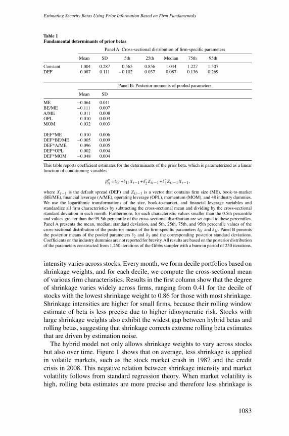
3.1 Fundamental determinants of betasTable 1 summarizes the relation between prior betas and firm fundamentals.10
Consistent with theoretical predictions, we find that all characteristics in theprior model are important determinants of beta. The negative coefficient on sizeindicates that small firms have higher betas than large firms, and the negativeloading on book-to-market implies that value firms are unconditionally lessrisky than growth firms. As predicted by Carlson, Fisher, and Giammarino(2004), we find that higher operating leverage leads to higher betas. Theloadings on the interaction terms between the default spread and the firmcharacteristics show how betas vary over the business cycle. The positivecoefficient on the interaction of the default spread and financial leverage isconsistent with the model of Livdan, Sapriza, and Zhang (2009), in which thedividends of firms with higher leverage are more strongly correlated with thebusiness cycle. Finally, we observe a large cross-sectional spread in the firm-specific parameter δ0i in the prior specification in Equation (4), which highlightsthe importance of also allowing for variation in betas unrelated to fundamentals.
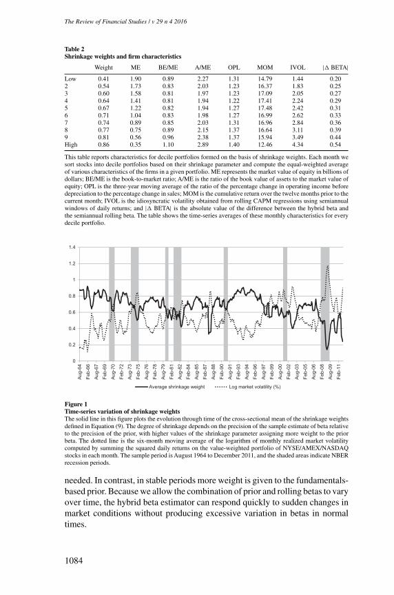
3.2 Variation in shrinkage weightsBy construction, the shrinkage parameter in (9) lies between zero and one,with higher values assigning more weight to the prior beta. In Table 2 werelate shrinkage weights to firm characteristics to examine how the shrinkage
10 For brevity, the coefficients on the 48 industry dummies are not reported. We find that most of the industrydummies contain significant prior information about the cross-sectional variation in betas.
1082
Estimating Security Betas Using Prior Information Based on Firm Fundamentals
Table 1Fundamental determinants of prior betas
Panel A: Cross-sectional distribution of firm-specific parameters
Mean SD 5th 25th Median 75th 95th
Constant 1.004 0.287 0.565 0.856 1.044 1.227 1.507DEF 0.087 0.111 – 0.102 0.037 0.087 0.136 0.269
Panel B: Posterior moments of pooled parameters
Mean SD
ME −0.064 0.011BE/ME −0.111 0.007A/ME 0.011 0.008OPL 0.010 0.003MOM 0.032 0.003
DEF*ME 0.010 0.006DEF*BE/ME −0.005 0.009DEF*A/ME 0.096 0.005DEF*OPL 0.002 0.004DEF*MOM −0.048 0.004
This table reports coefficient estimates for the determinants of the prior beta, which is parameterized as a linearfunction of conditioning variables
β∗it =δ0i +δ1iXt−1 +δ′2Zit−1 +δ′3Zit−1Xt−1,
where Xt−1 is the default spread (DEF) and Zit−1 is a vector that contains firm size (ME), book-to-market(BE/ME), financial leverage (A/ME), operating leverage (OPL), momentum (MOM), and 48 industry dummies.We use the logarithmic transformations of the size, book-to-market, and financial leverage variables andstandardize all firm characteristics by subtracting the cross-sectional mean and dividing by the cross-sectionalstandard deviation in each month. Furthermore, for each characteristic values smaller than the 0.5th percentileand values greater than the 99.5th percentile of the cross-sectional distribution are set equal to these percentiles.Panel A presents the mean, median, standard deviation, and 5th, 25th, 75th, and 95th percentile values of thecross-sectional distribution of the posterior means of the firm-specific parameters δ0i and δ1i . Panel B presentsthe posterior means of the pooled parameters δ2 and δ3 and the corresponding posterior standard deviations.Coefficients on the industry dummies are not reported for brevity.All results are based on the posterior distributionof the parameters constructed from 1,250 iterations of the Gibbs sampler with a burn-in period of 250 iterations.
intensity varies across stocks. Every month, we form decile portfolios based onshrinkage weights, and for each decile, we compute the cross-sectional meanof various firm characteristics. Results in the first column show that the degreeof shrinkage varies widely across firms, ranging from 0.41 for the decile ofstocks with the lowest shrinkage weight to 0.86 for those with most shrinkage.Shrinkage intensities are higher for small firms, because their rolling windowestimate of beta is less precise due to higher idiosyncratic risk. Stocks withlarge shrinkage weights also exhibit the widest gap between hybrid betas androlling betas, suggesting that shrinkage corrects extreme rolling beta estimatesthat are driven by estimation noise.
The hybrid model not only allows shrinkage weights to vary across stocksbut also over time. Figure 1 shows that on average, less shrinkage is appliedin volatile markets, such as the stock market crash in 1987 and the creditcrisis in 2008. This negative relation between shrinkage intensity and marketvolatility follows from standard regression theory. When market volatility ishigh, rolling beta estimates are more precise and therefore less shrinkage is
1083
The Review of Financial Studies / v 29 n 4 2016
Table 2Shrinkage weights and firm characteristics
Weight ME BE/ME A/ME OPL MOM IVOL | BETA|Low 0.41 1.90 0.89 2.27 1.31 14.79 1.44 0.202 0.54 1.73 0.83 2.03 1.23 16.37 1.83 0.253 0.60 1.58 0.81 1.97 1.23 17.09 2.05 0.274 0.64 1.41 0.81 1.94 1.22 17.41 2.24 0.295 0.67 1.22 0.82 1.94 1.27 17.48 2.42 0.316 0.71 1.04 0.83 1.98 1.27 16.99 2.62 0.337 0.74 0.89 0.85 2.03 1.31 16.96 2.84 0.368 0.77 0.75 0.89 2.15 1.37 16.64 3.11 0.399 0.81 0.56 0.96 2.38 1.37 15.94 3.49 0.44High 0.86 0.35 1.10 2.89 1.40 12.46 4.34 0.54
This table reports characteristics for decile portfolios formed on the basis of shrinkage weights. Each month wesort stocks into decile portfolios based on their shrinkage parameter and compute the equal-weighted averageof various characteristics of the firms in a given portfolio. ME represents the market value of equity in billions ofdollars; BE/ME is the book-to-market ratio; A/ME is the ratio of the book value of assets to the market value ofequity; OPL is the three-year moving average of the ratio of the percentage change in operating income beforedepreciation to the percentage change in sales; MOM is the cumulative return over the twelve months prior to thecurrent month; IVOL is the idiosyncratic volatility obtained from rolling CAPM regressions using semiannualwindows of daily returns; and | BETA| is the absolute value of the difference between the hybrid beta andthe semiannual rolling beta. The table shows the time-series averages of these monthly characteristics for everydecile portfolio.
0
0.2
0.4
0.6
0.8
1
1.2
1.4
Aug
-64
Feb-
66
Aug
-67
Feb-
69
Aug
-70
Feb-
72
Aug
-73
Feb-
75
Aug
-76
Feb-
78
Aug
-79
Feb-
81
Aug
-82
Feb-
84
Aug
-85
Feb-
87
Aug
-88
Feb-
90
Aug
-91
Feb-
93
Aug
-94
Feb-
96
Aug
-97
Feb-
99
Aug
-00
Feb-
02
Aug
-03
Feb-
05
Aug
-06
Feb-
08
Aug
-09
Feb-
11
Average shrinkage weight Log market volatility (%)
Figure 1Time-series variation of shrinkage weightsThe solid line in this figure plots the evolution through time of the cross-sectional mean of the shrinkage weightsdefined in Equation (9). The degree of shrinkage depends on the precision of the sample estimate of beta relativeto the precision of the prior, with higher values of the shrinkage parameter assigning more weight to the priorbeta. The dotted line is the six-month moving average of the logarithm of monthly realized market volatilitycomputed by summing the squared daily returns on the value-weighted portfolio of NYSE/AMEX/NASDAQstocks in each month. The sample period is August 1964 to December 2011, and the shaded areas indicate NBERrecession periods.
needed. In contrast, in stable periods more weight is given to the fundamentals-based prior. Because we allow the combination of prior and rolling betas to varyover time, the hybrid beta estimator can respond quickly to sudden changes inmarket conditions without producing excessive variation in betas in normaltimes.
1084
Estimating Security Betas Using Prior Information Based on Firm Fundamentals
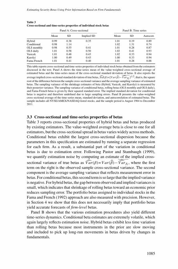
Table 3Cross-sectional and time-series properties of individual stock betas
Panel A: Cross-sectional Panel B: Time series
Mean SD Implied SD Mean SD Autocorr.
Hybrid 0.99 0.38 0.35 1.01 0.19 0.89Conditional 0.98 1.14 - 1.02 1.31 0.74OLS monthly 0.98 0.55 0.41 1.01 0.28 0.87OLS daily 1.01 0.58 0.50 1.02 0.41 0.93Vasicek 1.01 0.48 0.43 1.02 0.33 0.94Karolyi 1.00 0.49 0.43 1.00 0.33 0.94Fama-French 1.01 0.41 0.40 1.01 0.28 0.88
This table reports cross-sectional and time-series properties of individual stock betas obtained from the estimatorsdiscussed in the text. Panel A shows the time-series mean of the value-weighted cross-sectional average ofestimated betas and the time-series mean of the cross-sectional standard deviation of betas. It also reports the
average implied cross-sectional standard deviation of true betas, Std(β)= [V ar(β)−V arβi ]1/2, that is, the squareroot of the difference between the sample cross-sectional variance and the average sampling variance of estimatedbetas. The sampling variance of the shrinkage estimates of beta (Hybrid, Vasicek, and Karolyi) is measured bytheir posterior variance. The sampling variance of conditional betas, rolling betas (OLS monthly and OLS daily),and Fama-French betas is given by their squared standard error. The implied standard deviation for conditionalbetas is negative and therefore undefined due to large sampling errors. Panel B presents the value-weightedcross-sectional average of the time-series mean, standard deviation, and autocorrelation of estimated betas. Thesample includes all NYSE/AMEX/NASDAQ-listed stocks, and the sample period is August 1964 to December2011.
3.3 Cross-sectional and time-series properties of betasTable 3 reports cross-sectional properties of hybrid betas and betas producedby existing estimators. The value-weighted average beta is close to one for allestimators, but the cross-sectional spread in betas varies widely across methods.Conditional betas exhibit the largest cross-sectional dispersion because theparameters in this specification are estimated by running a separate regressionfor each firm. As a result, a substantial part of the variation in conditionalbetas is due to estimation error. Following Pastor and Stambaugh (1999),we quantify estimation noise by computing an estimate of the implied cross-
sectional variance of true betas as V ar(β)=V ar(β)−V arβi , where the firstterm on the right is the observed sample cross-sectional variance. The secondcomponent is the average sampling variance that reflects measurement error inbetas. For conditional betas, this second term is so large that the implied varianceis negative. For hybrid betas, the gap between observed and implied variances issmall, which indicates that shrinkage of rolling betas toward an economic priorreduces sampling error. The portfolio betas assigned to individual stocks in theFama and French (1992) approach are also measured with precision. However,in Section 4 we show that this does not necessarily imply that portfolio betasyield accurate forecasts of firm-level betas.
Panel B shows that the various estimation procedures also yield differenttime-series dynamics. Conditional beta estimates are extremely volatile, whichagain largely reflects estimation noise. Hybrid betas exhibit less time variationthan rolling betas because most instruments in the prior are slow movingand included to pick up long-run movements in betas driven by changes infundamentals.
1085
The Review of Financial Studies / v 29 n 4 2016
4. Out-of-Sample Beta Forecasts
In this section we run a horse race between the hybrid estimator and existingbeta estimators. Section 4.1 provides direct evidence on the merits of thehybrid approach by comparing its out-of-sample forecasting ability to that ofcompeting estimation techniques. In Section 4.2 we perform a cross-sectionalanalysis of forecast errors to gain more intuition about the results acrossdifferent types of stocks. Finally, Section 4.3 examines the performance ofvarious stripped-down versions of the hybrid model to identify the key driversof its forecasting power.
4.1 Predicting individual stock betasWe generate out-of-sample beta forecasts at the end of every month t using thefollowing procedure. First, we estimate each beta model using only data up tomonth t and take stock i’s beta as forecast for its beta at time t +k, which welabel βFit+k|t . We consider monthly, yearly, and five-year forecast horizons, forwhich k is equal to 1, 12, and 60, respectively. Subsequently, we compare thisforecast to the realized beta over the forecast interval that is computed usingreturn data from the start of month t +1 to the end of month t +k and denoted byβRit+k . We proceed by reestimating each model using data up to month t +1 toproduce a forecast for beta at time t +1+k. By repeating this procedure everymonth, we obtain a time series of out-of-sample beta forecasts.
We estimate the realized beta of stock i over the forecast interval k as
βRit+k≡CovRiM,t+k
V arRM,t+k=
∑k/
h=1 ri,t+hrM,t+h∑k/
h=1 r2M,t+h
, (10)
where CovRiM,t+k is the realized covariance between stock i and the market andV arRM,t+k is the realized market variance. These moments are computed usingthe continuously compounded returns ri,t+h and rM,t+h that are defined asthe difference in log prices sampled at interval , that is, pi,t+h−pi,t+(h−1)
andpM,t+h−pM,t+(h−1), respectively. We consider one-month, one-year, andfive-year window lengths k corresponding to the different forecast horizons thatwe examine. Andersen et al. (2006) demonstrate that a realized beta measureconstructed from high-frequency returns is a consistent estimator of the trueintegrated beta. In practice, however, market microstructure frictions, such asthe bid-ask bounce and nonsynchronous trading effects, put an upper limit onthe data frequency that can be used to estimate realized betas.
Because microstructure noise has a minor impact on liquid stocks, weuse intraday data to compute realized betas for the subset of stocks in oursample that are included in the S&P 100 index. Following Andersen et al.(2000), we estimate realized betas using 15-minute returns. We calculate high-frequency returns using transaction prices from the TAQ database. In particular,we construct equally spaced 15-minute returns by computing the logarithmicdifference in prices at or immediately before each 15-minute mark. We use the
1086
Estimating Security Betas Using Prior Information Based on Firm Fundamentals
liquid SPY exchange traded fund (ETF) that tracks the S&P 500 as a proxyfor the market index. Our sample of intraday returns extends from January2, 1996 to December 31, 2011. The out-of-sample period therefore starts inJanuary 1996, and the first beta forecasts for the S&P 100 stocks are obtainedby estimating the beta models that we consider using data up to December 1995.
We also study the forecasting ability of the beta estimators for the fullcross-section of NYSE/AMEX/NASDAQ-listed stocks and a longer out-of-sample period that starts in August 1984 and ends in December 2011.11
For this broad universe of stocks, we focus on one- and five-year forecasthorizons and compute realized betas using daily returns to mitigate biases dueto microstructure issues.12 However, by using lower frequency (daily) data, therealized beta estimates are less accurate. Andersen, Bollerslev, and Meddahi(2005) analyze this complication in the context of volatility forecasting anddemonstrate that because of noise in the realized volatility used as proxy for thetrue latent volatility, the true predictive accuracy of forecasts is underestimated.Measurement error in realized betas is particularly a concern for small stocksbecause their returns are more sensitive to microstructure noise. We thereforeevaluate the forecast accuracy of beta estimators by computing value-weightedmean squared errors in each out-of-sample period
MSEt,t+k =Nt∑i=1
wit (βRit+k−βFit+k|t )2, (11)
where Nt is the number of stocks in the sample at time t and wit is the weightof each stock.13
We use two procedures to evaluate the statistical significance of differencesin MSEs generated by the hybrid estimator (MSE0) and a competing approach(MSEj ). The first method is the Diebold and Mariano (1995) test of equalpredictive ability, which is a t-test that takes the form
DMj,k =dj,k√σ 2d /P
, (12)
where dj,k = 1P
∑T−kt=Q dj,t+k with dj,t+k =MSEjt,t+k−MSE0
t,t+k , Q is the lengthof the in-sample estimation window, and P is the number of out-of-sampleobservations. σ 2
d is a consistent estimate of the long-run variance of the loss
11 This start date implies that the first forecasts are formed using the first 20 years of data to estimate the models.The choice of an initial 20-year estimation period is common in the literature (see, e.g., Goyal and Welch 2008).
12 We omit the monthly horizon because realized betas computed from one month of daily returns are very noisy.
13 We confirm empirically that the standard errors of realized beta estimates of small stocks are much larger thanthose of big stocks. Because value weighting mitigates the impact of noise in realized betas of small stocks,it allows for a more reliable evaluation of forecasting performance than equal weighting. Indeed, for all betaestimators we find that value-weighted MSEs are smaller than equal-weighted MSEs. However, the ranking ofbeta estimators is the same whether the ranking is done using equal-weighted or value-weighted MSEs.
1087
The Review of Financial Studies / v 29 n 4 2016
differences dj,t+k . Because we make a new prediction every month, forecasterrors for the one- and five-year horizons are based on overlapping out-of-sample periods. We use two different HAC estimators of σ 2
d to account for theautocorrelation in forecast errors caused by the overlapping data. First, we usethe Newey and West (1987) estimator with bandwidth set equal to 1.5 times theforecast horizon k. We let the maximal lag length exceed the forecast horizonbecause the Bartlett kernel underweights higher-order autocorrelations. Wealso report results based on the HAC estimator of West (1997), which capturesthe autocorrelation structure by fitting an MA model to the residual series ofthe forecasting regression. Consequently, higher-order autocorrelations are notdownweighted and the number of lags is set equal to k−1.14
The second approach that we use to evaluate significance is the test of equalfinite-sample predictive accuracy proposed by Giacomini and White (2006;denoted GW).15 This procedure allows us to test for conditional predictiveability and accounts for the effect of parameter estimation uncertainty onrelative forecast accuracy.16 The null hypothesis of the GW test is
H0 :E[MSEjt,t+k−MSE0t,t+k|It−1]=0, (13)
where It−1 is the information set at time t−1. The main idea of testing forconditional predictive ability is to test whether currently available informationcan be used to predict which forecasting method leads to smaller forecastingerrors in the out-of-sample period. In our implementation of the test, we selecta q-dimensional vector of elements from the information set that includes aconstant and the loss differential in the last period. The GW test statistic isa Wald-type statistic, which follows a χ2
q distribution under the null of equalpredictive ability. We compute the test statistic using a Newey-West estimateof the variance with bandwidth equal to 1.5 times the forecast horizon.
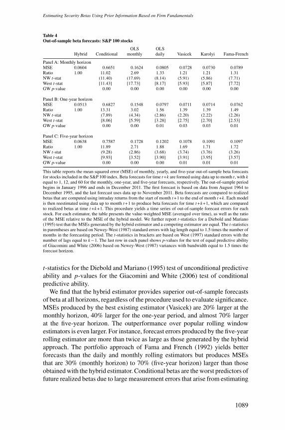
4.1.1 S&P 100 stocks. Table 4 reports results for the S&P 100 stocks forwhich we compute realized betas using intraday returns. For each estimator,we present the value-weighted MSE, averaged over time, as well as the ratioof the MSE relative to the MSE of the hybrid model. In addition, we report
14 For additional robustness, we also compute variances using a rectangular kernel with bandwidth k−1 and thesmall-sample adjustment of Harvey, Leybourne, and Newbold (1997). Moreover, we compute p-values for theDiebold and Mariano (1995) test statistic based on a non-parametric bootstrap along the lines of White (2000).Both methods lead to results similar to those based on the Newey and West (1987) and West (1997) HACestimators.
15 In theory, the asymptotics of Giacomini and White (2006) no longer apply when a recursive scheme is used toestimate the model parameters. However, Clark and McCracken (2013) present Monte Carlo evidence showingthat, in practice, the test works about as well for the recursive scheme as for the rolling scheme.
16 The object of evaluation in the procedure of Giacomini and White (2006) is the forecasting method, whichnot only encompasses the forecasting model but also includes the estimation procedure and the data used forestimation. As a result, this test is well suited for MSE comparisons in our setting, which involves modelsestimated using various methods (Bayesian and frequentist) and different window lengths and data frequencies(daily and monthly).
1088
Estimating Security Betas Using Prior Information Based on Firm Fundamentals
Table 4Out-of-sample beta forecasts: S&P 100 stocks
OLS OLSHybrid Conditional monthly daily Vasicek Karolyi Fama-French
Panel A: Monthly horizonMSE 0.0604 0.6651 0.1624 0.0805 0.0728 0.0730 0.0789Ratio 1.00 11.02 2.69 1.33 1.21 1.21 1.31NW t-stat (11.40) (17.69) (8.14) (5.91) (5.86) (7.71)West t-stat [11.43] [17.73] [8.17] [5.93] [5.87] [7.72]GW p-value 0.00 0.00 0.00 0.00 0.00 0.00
Panel B: One-year horizonMSE 0.0513 0.6827 0.1548 0.0797 0.0711 0.0714 0.0762Ratio 1.00 13.31 3.02 1.56 1.39 1.39 1.49NW t-stat (7.89) (4.34) (2.86) (2.20) (2.22) (2.26)West t-stat [8.06] [5.59] [3.28] [2.75] [2.70] [2.53]GW p-value 0.00 0.00 0.01 0.03 0.03 0.01
Panel C: Five-year horizonMSE 0.0638 0.7587 0.1728 0.1202 0.1078 0.1091 0.1097Ratio 1.00 11.89 2.71 1.88 1.69 1.71 1.72NW t-stat (9.28) (2.86) (3.68) (3.74) (3.76) (3.26)West t-stat [9.93] [3.52] [3.90] [3.91] [3.95] [3.57]GW p-value 0.00 0.00 0.00 0.01 0.01 0.01
This table reports the mean squared error (MSE) of monthly, yearly, and five-year out-of-sample beta forecastsfor stocks included in the S&P 100 index. Beta forecasts for time t +k are formed using data up to month t , with kequal to 1, 12, and 60 for the monthly, one-year, and five-year forecasts, respectively. The out-of-sample periodbegins in January 1996 and ends in December 2011. The first forecast is based on data from August 1964 toDecember 1995, and the last forecast uses data up to November 2011. Beta forecasts are compared to realizedbetas that are computed using intraday returns from the start of month t +1 to the end of month t +k. Each modelis then reestimated using data up to month t +1 to produce beta forecasts for time t +k+1, which are comparedto realized betas at time t +k+1. This procedure yields a time series of out-of-sample forecast errors for eachstock. For each estimator, the table presents the value-weighted MSE (averaged over time), as well as the ratioof the MSE relative to the MSE of the hybrid model. We further report t-statistics for a Diebold and Mariano(1995) test that the MSEs generated by the hybrid estimator and a competing estimator are equal. The t-statisticsin parentheses are based on Newey-West (1987) standard errors with lag length equal to 1.5 times the number ofmonths in the forecasting period. The t-statistics in brackets are based on West (1997) standard errors with thenumber of lags equal to k−1. The last row in each panel shows p-values for the test of equal predictive abilityof Giacomini and White (2006) based on Newey-West (1987) variances with bandwidth equal to 1.5 times theforecast horizon.
t-statistics for the Diebold and Mariano (1995) test of unconditional predictiveability and p-values for the Giacomini and White (2006) test of conditionalpredictive ability.
We find that the hybrid estimator provides superior out-of-sample forecastsof beta at all horizons, regardless of the procedure used to evaluate significance.MSEs produced by the best existing estimator (Vasicek) are 20% larger at themonthly horizon, 40% larger for the one-year period, and almost 70% largerat the five-year horizon. The outperformance over popular rolling windowestimators is even larger. For instance, forecast errors produced by the five-yearrolling estimator are more than twice as large as those generated by the hybridapproach. The portfolio approach of Fama and French (1992) yields betterforecasts than the daily and monthly rolling estimators but produces MSEsthat are 30% (monthly horizon) to 70% (five-year horizon) larger than thoseobtained with the hybrid estimator. Conditional betas are the worst predictors offuture realized betas due to large measurement errors that arise from estimating
1089
The Review of Financial Studies / v 29 n 4 2016
Table 5Out-of-sample beta forecasts: All stocks
OLS OLSHybrid Conditional monthly daily Vasicek Karolyi Fama-French
Panel A: One-year horizonMSE 0.0970 4.4591 0.1968 0.1153 0.1077 0.1073 0.1136Ratio 1.00 45.97 2.03 1.19 1.11 1.11 1.17NW t-stat (4.13) (5.46) (3.53) (2.08) (2.10) (2.46)West t-stat [4.51] [6.58] [3.21] [2.01] [1.98] [2.75]GW p-value 0.00 0.00 0.00 0.03 0.03 0.01
Panel B: Five-year horizonMSE 0.0946 3.9621 0.1948 0.1431 0.1248 0.1257 0.1259Ratio 1.00 41.89 2.06 1.51 1.32 1.33 1.33NW t-stat (6.09) (2.84) (6.73) (4.47) (4.48) (3.40)West t-stat [5.25] [3.91] [4.53] [2.58] [2.93] [3.10]GW p-value 0.00 0.01 0.00 0.00 0.00 0.00
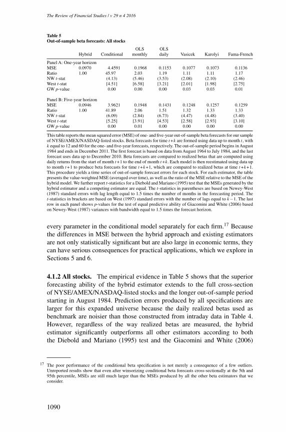
This table reports the mean squared error (MSE) of one- and five-year out-of-sample beta forecasts for our sampleof NYSE/AMEX/NASDAQ-listed stocks. Beta forecasts for time t +k are formed using data up to month t , withk equal to 12 and 60 for the one- and five-year forecasts, respectively. The out-of-sample period begins in August1984 and ends in December 2011. The first forecast is based on data from August 1964 to July 1984, and the lastforecast uses data up to December 2010. Beta forecasts are compared to realized betas that are computed usingdaily returns from the start of month t +1 to the end of month t +k. Each model is then reestimated using data upto month t +1 to produce beta forecasts for time t +k+1, which are compared to realized betas at time t +k+1.This procedure yields a time series of out-of-sample forecast errors for each stock. For each estimator, the tablepresents the value-weighted MSE (averaged over time), as well as the ratio of the MSE relative to the MSE of thehybrid model. We further report t-statistics for a Diebold and Mariano (1995) test that the MSEs generated by thehybrid estimator and a competing estimator are equal. The t-statistics in parentheses are based on Newey-West(1987) standard errors with lag length equal to 1.5 times the number of months in the forecasting period. Thet-statistics in brackets are based on West (1997) standard errors with the number of lags equal to k−1. The lastrow in each panel shows p-values for the test of equal predictive ability of Giacomini and White (2006) basedon Newey-West (1987) variances with bandwidth equal to 1.5 times the forecast horizon.
every parameter in the conditional model separately for each firm.17 Becausethe differences in MSE between the hybrid approach and existing estimatorsare not only statistically significant but are also large in economic terms, theycan have serious consequences for practical applications, which we explore inSections 5 and 6.
4.1.2 All stocks. The empirical evidence in Table 5 shows that the superiorforecasting ability of the hybrid estimator extends to the full cross-sectionof NYSE/AMEX/NASDAQ-listed stocks and the longer out-of-sample periodstarting in August 1984. Prediction errors produced by all specifications arelarger for this expanded universe because the daily realized betas used asbenchmark are noisier than those constructed from intraday data in Table 4.However, regardless of the way realized betas are measured, the hybridestimator significantly outperforms all other estimators according to boththe Diebold and Mariano (1995) test and the Giacomini and White (2006)
17 The poor performance of the conditional beta specification is not merely a consequence of a few outliers.Unreported results show that even after winsorizing conditional beta forecasts cross-sectionally at the 5th and95th percentile, MSEs are still much larger than the MSEs produced by all the other beta estimators that weconsider.
1090
Estimating Security Betas Using Prior Information Based on Firm Fundamentals
procedure. The other approaches that involve some form of shrinkage (Vasicekand Karolyi) and the portfolio procedure of Fama and French (1992) yieldbetter predictions of beta than simple rolling estimators, but they do not matchthe forecasting performance of the hybrid model.
4.2 Cross-sectional analysis of forecast errorsThe forecasting results in the previous section raise the question of why thehybrid approach works better than existing beta estimators. To answer thisquestion, we first need to identify the type of stocks for which the hybridestimator works particularly well. The descriptive results in Table 2 suggest thatshrinkage is most beneficial for stocks with extreme sample estimates of betastemming from large measurement errors. We test this conjecture as follows.At the end of each month, stocks are sorted into decile portfolios based ontheir predicted beta. Ex ante portfolio betas are measured as the value-weightedaverage of these beta forecasts. Ex post portfolio betas are estimated by runninga regression of daily portfolio returns on a constant and the market return overthe next year. Forecast errors are defined as the difference between ex post andex ante portfolio betas.
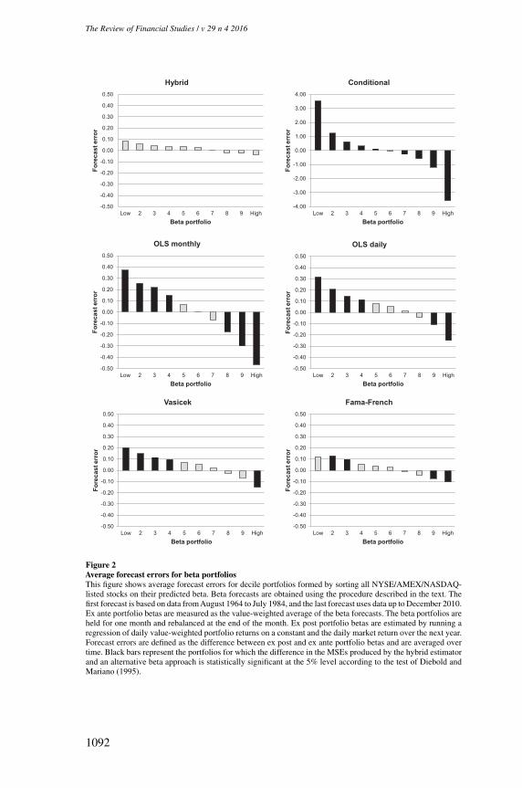
Figure 2 plots the average forecast error for each beta decile.18 The black barsrepresent the deciles for which the hybrid estimator produces significantly lowerMSEs than a competing approach according to the Diebold and Mariano (1995)test. A clear pattern emerges: all existing estimators significantly underestimatelow betas and overestimate high betas. Average forecast errors for the dailyrolling window estimator range from 0.32 for the low-beta decile to -0.25 forthe decile of high-beta stocks. The five-year rolling estimator based on monthlyreturns performs even worse as it underestimates the beta of stocks in the bottomdecile by 0.37 and overestimates the beta of the top portfolio by 0.47. TheVasicek and Karolyi estimators dampen only part of the noise in rolling betaestimates. Forecast errors for the low-beta deciles remain significantly positive,while the high-beta portfolios still exhibit substantial negative forecast errors.The estimation approach of Fama and French (1992) does better than theseconventional shrinkage estimators. An important downside of this procedureis that it ignores the cross-sectional heterogeneity in betas within each of thesize-beta portfolios stocks are sorted into. Consequently, even if the betas of thesize-beta sorted portfolios themselves are unbiased, assigning these portfoliobetas to individual stocks induces a bias in firm-level betas that leads to higherMSEs in the firm-level forecasts in Tables 4 and 5. However, this problem isless severe in the portfolio-level test in Figure 2 because upward and downwardbiases in firm-level betas tend to cancel out at the portfolio level. Nevertheless,the Fama and French (1992) method still yields sizeable forecast errors for high-and low-beta deciles. In contrast, prediction errors produced by the hybrid
18 We omit the Karolyi approach to save space. The results are very similar to those for the Vasicek estimator.
1091
The Review of Financial Studies / v 29 n 4 2016
-0.50
-0.40
-0.30
-0.20
-0.10
0.00
0.10
0.20
0.30
0.40
0.50
Low 2 3 4 5 6 7 8 9 High
Fore
cast
err
or
Beta portfolio
Hybrid
-4.00
-3.00
-2.00
-1.00
0.00
1.00
2.00
3.00
4.00
Low 2 3 4 5 6 7 8 9 High
Fore
cast
err
or
Beta portfolio
Conditional
-0.50
-0.40
-0.30
-0.20
-0.10
0.00
0.10
0.20
0.30
0.40
0.50
Low 2 3 4 5 6 7 8 9 High
Fore
cast
err
or
Beta portfolio
OLS monthly
-0.50
-0.40
-0.30
-0.20
-0.10
0.00
0.10
0.20
0.30
0.40
0.50
Low 2 3 4 5 6 7 8 9 High
Fore
cast
err
or
Beta portfolio
OLS daily
-0.50
-0.40
-0.30
-0.20
-0.10
0.00
0.10
0.20
0.30
0.40
0.50
Low 2 3 4 5 6 7 8 9 High
Fore
cast
err
or
Beta portfolio
Vasicek
-0.50
-0.40
-0.30
-0.20
-0.10
0.00
0.10
0.20
0.30
0.40
0.50
Low 2 3 4 5 6 7 8 9 High
Fore
cast
err
or
Beta portfolio
Fama-French
Figure 2Average forecast errors for beta portfoliosThis figure shows average forecast errors for decile portfolios formed by sorting all NYSE/AMEX/NASDAQ-listed stocks on their predicted beta. Beta forecasts are obtained using the procedure described in the text. Thefirst forecast is based on data from August 1964 to July 1984, and the last forecast uses data up to December 2010.Ex ante portfolio betas are measured as the value-weighted average of the beta forecasts. The beta portfolios areheld for one month and rebalanced at the end of the month. Ex post portfolio betas are estimated by running aregression of daily value-weighted portfolio returns on a constant and the daily market return over the next year.Forecast errors are defined as the difference between ex post and ex ante portfolio betas and are averaged overtime. Black bars represent the portfolios for which the difference in the MSEs produced by the hybrid estimatorand an alternative beta approach is statistically significant at the 5% level according to the test of Diebold andMariano (1995).
1092
Estimating Security Betas Using Prior Information Based on Firm Fundamentals
estimator are smaller and do not exhibit such a pronounced pattern acrossdeciles. The Diebold and Mariano (1995) test confirms that existing methodsgenerate significantly larger MSEs for the extreme beta portfolios than thehybrid model.
Why does the hybrid estimator perform better for stocks with extreme betaestimates than other methods? We answer this question by relating the cross-sectional spread in betas to measurement error. More specifically, we regressthe squared deviation of beta forecasts from their cross-sectional mean on a setof firm characteristics and on a firm’s idiosyncratic volatility. Our motivationfor doing so is that from a theoretical point of view, we do not expect a relationbetween idiosyncratic risk and the spread in betas after controlling for firmcharacteristics that are known to drive variation in betas. Empirically, however,a positive relation may exist because higher idiosyncratic risk increases thestandard error of beta estimates (all else equal), leading to more extremesample estimates of beta. However, with shrinkage, higher idiosyncratic riskand therefore noisier sample betas imply that less weight is given to the sampleestimate of beta and more weight is assigned to the prior. Thus, if shrinkagereduces measurement error in betas, we expect the positive relation betweenidiosyncratic risk and dispersion in betas to be weaker for shrinkage estimatesof beta than for sample estimates of beta. The more precise the prior is, the moreeffective the shrinkage, and the weaker the relation between idiosyncratic riskand cross-sectional variation in betas will be.
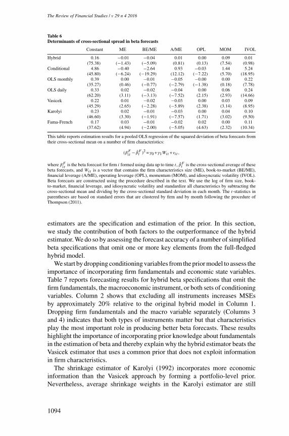
The results reported in Table 6 confirm that existing estimators generatemore extreme betas for stocks with higher idiosyncratic volatility, evenafter controlling for various firm characteristics. The standardized coefficienton idiosyncratic risk is largest for standard rolling window betas and forconditional betas estimated using time-series regressions. The Vasicek andKarolyi shrinkage methods and the Fama-French approach do a better job butstill produce extreme beta estimates driven by sampling error. In contrast, forthe hybrid estimator, we do not find a significant relation between idiosyncraticrisk and cross-sectional spread in betas, which indicates that the cross-sectionaldispersion in hybrid betas is largely unrelated to measurement noise.
In sum, we find that the hybrid model produces more accurate beta forecaststhan alternative approaches because shrinkage toward a fundamentals-basedprior corrects the tendency of rolling sample estimators to overpredict at highbeta estimates and underpredict at low estimates. Existing shrinkage estimatorsand methods that group stocks into portfolios offer only limited improvementover rolling estimators and yield significantly larger prediction errors than thehybrid method.
4.3 Decomposition of hybrid beta forecasting performanceThe analysis in the preceding section leaves us with one final question: whyis shrinkage in the hybrid model more effective than in traditional methods?The main features of the hybrid model that set it apart from other shrinkage
1093
The Review of Financial Studies / v 29 n 4 2016
Table 6Determinants of cross-sectional spread in beta forecasts
Constant ME BE/ME A/ME OPL MOM IVOL
Hybrid 0.16 −0.01 −0.04 0.01 0.00 0.09 0.01(75.38) (−1.43) (−5.09) (0.81) (0.13) (7.54) (0.98)
Conditional 4.86 −0.40 −2.64 0.93 −0.03 1.44 5.24(45.80) (−6.24) (−19.29) (12.12) (−7.22) (5.70) (18.95)
OLS monthly 0.39 0.00 −0.01 −0.05 −0.00 0.00 0.22(35.27) (0.46) (−0.77) (−2.79) (−1.38) (0.18) (7.78)
OLS daily 0.33 0.02 −0.02 −0.04 0.00 0.06 0.24(62.20) (3.11) (−3.13) (−7.52) (2.15) (2.93) (14.66)
Vasicek 0.22 0.01 −0.02 −0.03 0.00 0.03 0.09(45.29) (2.65) (−2.28) (−5.89) (2.38) (3.14) (8.95)
Karolyi 0.23 0.02 −0.01 −0.03 0.00 0.04 0.10(46.60) (3.30) (−1.91) (−7.57) (1.71) (3.02) (9.50)
Fama-French 0.17 0.03 −0.01 −0.02 0.02 0.00 0.11(37.62) (4.94) (−2.00) (−5.05) (4.63) (2.32) (10.34)
This table reports estimation results for a pooled OLS regression of the squared deviation of beta forecasts fromtheir cross-sectional mean on a number of firm characteristics:
(βFit −βFt )2 =γ0 +γ1Wit +νit ,
where βFit
is the beta forecast for firm i formed using data up to time t , βFt is the cross-sectional average of thesebeta forecasts, and Wit is a vector that contains the firm characteristics size (ME), book-to-market (BE/ME),financial leverage (A/ME), operating leverage (OPL), momentum (MOM), and idiosyncratic volatility (IVOL).Beta forecasts are constructed using the procedure described in the text. We use the log of firm size, book-to-market, financial leverage, and idiosyncratic volatility and standardize all characteristics by subtracting thecross-sectional mean and dividing by the cross-sectional standard deviation in each month. The t-statistics inparentheses are based on standard errors that are clustered by firm and by month following the procedure ofThompson (2011).
estimators are the specification and estimation of the prior. In this section,we study the contribution of both factors to the outperformance of the hybridestimator. We do so by assessing the forecast accuracy of a number of simplifiedbeta specifications that omit one or more key elements from the full-fledgedhybrid model.
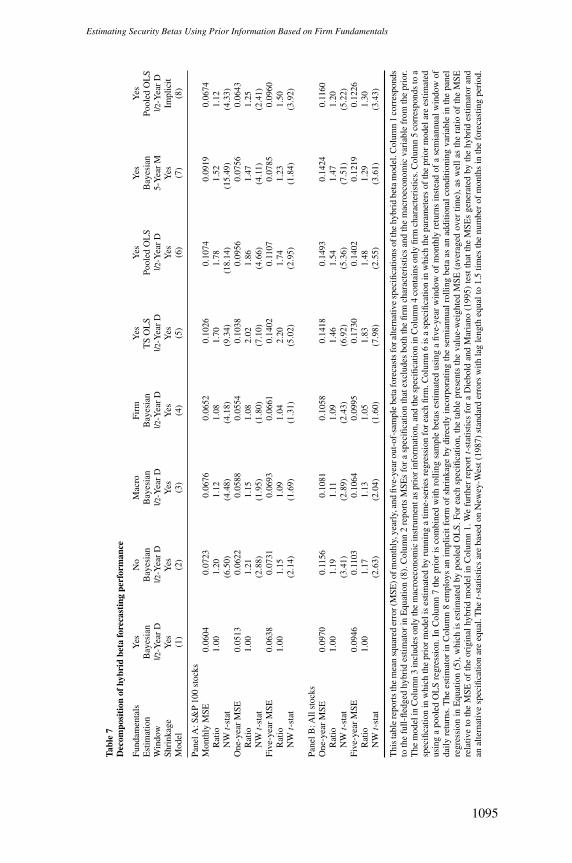
We start by dropping conditioning variables from the prior model to assess theimportance of incorporating firm fundamentals and economic state variables.Table 7 reports forecasting results for hybrid beta specifications that omit thefirm fundamentals, the macroeconomic instrument, or both sets of conditioningvariables. Column 2 shows that excluding all instruments increases MSEsby approximately 20% relative to the original hybrid model in Column 1.Dropping firm fundamentals and the macro variable separately (Columns 3and 4) indicates that both types of instruments matter but that characteristicsplay the most important role in producing better beta forecasts. These resultshighlight the importance of incorporating prior knowledge about fundamentalsin the estimation of beta and thereby explain why the hybrid estimator beats theVasicek estimator that uses a common prior that does not exploit informationin firm characteristics.
The shrinkage estimator of Karolyi (1992) incorporates more economicinformation than the Vasicek approach by forming a portfolio-level prior.Nevertheless, average shrinkage weights in the Karolyi estimator are still
1094
Estimating Security Betas Using Prior Information Based on Firm Fundamentals
Tabl
e7
Dec
ompo
siti
onof
hybr
idbe
tafo
reca
stin
gpe
rfor
man
ce
Fund
amen
tals
Yes
No
Mac
roFi
rmY
esY
esY
esY
esE
stim
atio
nB
ayes
ian
Bay
esia
nB
ayes
ian
Bay
esia
nT
SO
LS
Pool
edO
LS
Bay
esia
nPo
oled
OL
SW
indo
w1 /2
-Yea
rD
1 /2-Y
ear
D1 /2
-Yea
rD
1 /2-Y
ear
D1 /2
-Yea
rD
1 /2-Y
ear
D5-
Yea
rM
1 /2-Y
ear
DSh
rink
age
Yes
Yes
Yes
Yes
Yes
Yes
Yes
Impl
icit
Mod
el(1
)(2
)(3
)(4
)(5
)(6
)(7
)(8
)
Pane
lA:S
&P
100
stoc
ksM
onth
lyM
SE0.
0604
0.07
230.
0676
0.06
520.
1026
0.10
740.
0919
0.06
74R
atio
1.00
1.20
1.12
1.08
1.70
1.78
1.52
1.12
NW
t-st
at(6.5
0)(4.4
8)(4.1
8)(9.3
4)(1
8.14
)(1
5.49
)(4.3
3)O
ne-y
ear
MSE
0.05
130.
0622
0.05
880.
0554
0.10
380.
0956
0.07
560.
0643
Rat
io1.
001.
211.
151.
082.
021.
861.
471.
25N
Wt-
stat
(2.8
8)(1.9
5)(1.8
0)(7.1
0)(4.6
6)(4.1
1)(2.4
1)Fi
ve-y
ear
MSE
0.06
380.
0731
0.06
930.
0661
0.14
020.
1107
0.07
850.
0960
Rat
io1.
001.
151.
091.
042.
201.
741.
231.
50N
Wt-
stat
(2.1
4)(1.6
9)(1.3
1)(5.0
2)(2.9
5)(1.8
4)(3.9
2)
Pane
lB:A
llst
ocks
One
-yea
rM
SE0.
0970
0.11
560.
1081
0.10
580.
1418
0.14
930.
1424
0.11
60R
atio
1.00
1.19
1.11
1.09
1.46
1.54
1.47
1.20
NW
t-st
at(3.4
1)(2.8
9)(2.4
3)(6.9
2)(5.3
6)(7.5
1)(5.2
2)Fi
ve-y
ear
MSE
0.09
460.
1103
0.10
640.
0995
0.17
300.
1402
0.12
190.
1226
Rat
io1.
001.
171.
131.
051.
831.
481.
291.
30N
Wt-
stat
(2.6
3)(2.0
4)(1.6
0)(7.9
8)(2.5
5)(3.6
1)(3.4
3)
Thi
sta
ble
repo
rts
the
mea
nsq
uare
der
ror(
MSE
)ofm
onth
ly,y
earl
y,an
dfiv
e-ye
arou
t-of
-sam
ple
beta
fore
cast
sfo
ralte
rnat
ive
spec
ifica
tions
ofth
ehy
brid
beta
mod
el.C
olum
n1
corr
espo
nds
toth
efu
ll-fle
dged
hybr
ides
timat
orin
Equ
atio
n(8
).C
olum
n2
repo
rts
MSE
sfo
ra
spec
ifica
tion
that
excl
udes
both
the
firm
char
acte
rist
ics
and
the
mac
roec
onom
icva
riab
lefr
omth
epr
ior.
The
mod
elin
Col
umn
3in
clud
eson
lyth
em
acro
econ
omic
inst
rum
enta
spr
iori
nfor
mat
ion,
and
the
spec
ifica
tion
inC
olum
n4
cont
ains
only
firm
char
acte
rist
ics.
Col
umn
5co
rres
pond
sto
asp
ecifi
catio
nin
whi
chth
epr
ior
mod
elis
estim
ated
byru
nnin
ga
time-
seri
esre
gres
sion
for
each
firm
.Col
umn
6is
asp
ecifi
catio
nin
whi
chth
epa
ram
eter
sof
the
prio
rm
odel
are
estim
ated
usin
ga
pool
edO
LS
regr
essi
on.I
nC
olum
n7
the
prio
ris
com
bine
dw
ithro
lling
sam
ple
beta
ses
timat
edus
ing
afiv
e-ye
arw
indo
wof
mon
thly
retu
rns
inst
ead
ofa
sem
iann
ualw
indo
wof
daily
retu
rns.
The
estim
ator
inC
olum
n8
empl
oys
anim
plic
itfo
rmof
shri
nkag
eby
dire
ctly
inco
rpor
atin
gth
ese
mia
nnua
lrol
ling
beta
asan
addi
tiona
lcon
ditio
ning
vari
able
inth
epa
nel
regr
essi
onin
Equ
atio
n(5
),w
hich
ises
timat
edby
pool
edO
LS.
For
each
spec
ifica
tion,
the
tabl
epr
esen
tsth
eva
lue-
wei
ghte
dM
SE(a
vera
ged
over
time)
,as
wel
las
the
ratio
ofth
eM
SEre
lativ
eto
the
MSE
ofth
eor
igin
alhy
brid
mod
elin
Col
umn
1.W
efu
rthe
rre
port
t-st
atis
tics
for
aD
iebo
ldan
dM
aria
no(1
995)
test
that
the
MSE
sge
nera
ted
byth
ehy
brid
estim
ator
and
anal
tern
ativ
esp
ecifi
catio
nar
eeq
ual.
The
t-st
atis
tics
are
base
don
New
ey-W
est(
1987
)st
anda
rder
rors
with
lag
leng
theq
ualt
o1.
5tim
esth
enu
mbe
rof
mon
ths
inth
efo
reca
stin
gpe
riod
.
1095
The Review of Financial Studies / v 29 n 4 2016
lower than in the hybrid approach (0.20 versus 0.65, respectively) becausegrouping stocks into portfolios leads to a loss of information in firm-levelbetas.19 Specifically, in the Karolyi approach, the prior variance is computedas the cross-sectional variance of beta within each of the 48 industries definedby Fama and French (1997). If industry classification were the only relevantdeterminant of beta, cross-sectional variation in betas within each industryportfolio would be small and the prior would receive a large weight. In practice,however, industry classification is only one of many potential drivers of betaand intra-industry dispersion in betas is large. Consequently, prior precision islow and relatively little shrinkage is applied.
Next, we shed more light on the importance of the procedure used to estimatethe prior model. Prior betas in the Vasicek and Karolyi methods are estimatedusing an OLS regression for each stock or portfolio, whereas prior betas in thehybrid model are obtained from a Bayesian panel regression. We demonstratethe benefits of the Bayesian procedure by studying the forecasting performanceof hybrid beta specifications in which the fundamentals-based prior is estimatedusing either time-series or pooled OLS regressions. Column 5 in Table 7 showsthat estimating the prior using time-series regressions (i.e., using conditionalbetas as prior) yields significantly larger forecast errors than those generatedby the original hybrid model in Column 1 at both long and short horizons.Column 6 shows that estimating the prior using a pooled OLS regression alsoyields forecast errors that are more than 50% larger than those for the modelestimated using Bayesian methods.
The main difference between the pooled model in Column 6 and the hybridmodel in Column 1 is the δ0i coefficient on the unscaled market factor in theprior specification in Equation (5), which is assumed to be constant acrossfirms in the pooled OLS estimation. In contrast, in the Bayesian approach thisparameter is treated as firm specific and captures cross-sectional heterogeneityin betas unrelated to the fundamentals included in the prior model. The largecross-sectional spread in δ0i in Table 1 highlights the importance of allowingfor this flexibility in the prior to reduce misspecification bias.
In addition to shrinking rolling betas toward an economic prior, our hybridapproach differs from the widely used procedure of Fama and MacBeth (1973)by estimating the rolling sample betas using a semiannual window of dailyreturns instead of a five-year window of monthly returns. We quantify theimpact of data frequency and window length on the forecasting performanceof the hybrid estimator by combining fundamentals-based prior betas with
19 Apart from a difference in prior precision, the only other possible reason for the lower shrinkage weights inthe Vasicek and Karolyi methods is the precision of the rolling beta. The rolling beta in the hybrid model isestimated over a shorter (semiannual) window than the one-year beta used in the Vasicek and Karolyi estimators.Estimating Vasicek and Karolyi betas using a semiannual window leads to slightly higher shrinkage weights(0.24 for Vasicek and 0.27 for Karolyi), but this increase in shrinkage intensities does not translate into betterbeta forecasts.
1096
Estimating Security Betas Using Prior Information Based on Firm Fundamentals
five-year rolling betas estimated using monthly returns. The results in Column7 of Table 7 show that the use of five-year monthly rolling betas leads toa sharp increase in forecast errors. MSEs for the one-month and one-yearforecasts are about 50% higher than those for the original hybrid model withdaily rolling sample betas, and five-year MSEs increase by 25%. These findingsare consistent with the work of Andersen et al. (2006), who show that the use ofhigher-frequency returns increases the precision of beta estimates. Moreover,because of the shorter estimation window, the rolling betas in the hybrid modelare timelier and thus better suited to pick up short-term fluctuations in betas.20
Finally, we consider a specification that employs an implicit form ofshrinkage as an alternative to the formal shrinkage framework in Equation(8). This simplified model directly incorporates the semiannual rolling beta asan additional conditioning variable in the panel regression in Equation (5) andis estimated by pooled OLS. Results in the last column of Table 7 show thatthis model underperforms the full-fledged hybrid approach at all horizons. Thereasons for this underperformance are twofold. First, the model does not allowfor firm-specific shrinkage because the loading on the rolling beta is pooledacross stocks. Second, including rolling betas in the pooled regression does notadequately capture the effect of omitted conditioning variables, because it isunlikely that the unobserved heterogeneity in betas is an exact linear function ofrolling betas. Ghysels (1998) and Harvey (2001) demonstrate that conditionalbetas can be biased when the set of conditioning variables is incomplete orwhen the functional form of conditional expectations is misspecified.
In sum, based on the results in Table 7, we identify three reasons for theoutperformance of the hybrid beta estimator over existing estimators. First, byassigning a unique prior to each firm that incorporates a broad set of economicconditioning information, the hybrid model is more effective in reducingestimation noise in betas than conventional shrinkage estimators. Second, theBayesian approach used to estimate the fundamentals-based prior yields a betterbias-variance trade-off than frequentist estimation methods, because it allowsfor firm-level heterogeneity in some parameters of the prior model to reducebias, while pooling other parameters to increase precision. Third, by using asemiannual estimation window of daily returns instead of a five-year windowof monthly returns, the rolling betas in the hybrid model strike a better balancebetween timeliness and efficiency than those obtained from the classic rollingsample estimator of Fama and MacBeth (1973).
20 We disentangle the effects of the different data frequency and window length by considering a hybrid model thatuses five-year rolling betas estimated with daily returns. Unreported results show that estimating rolling samplebetas using a five-year window of monthly returns instead of a five-year window of daily returns increases MSEsby roughly 30% at all forecast horizons. Furthermore, we find that choosing a five-year window of daily returnsinstead of a semiannual window increases one-month MSEs by 30%, one-year MSEs by 20%, and five-yearMSEs by 5%.
1097
The Review of Financial Studies / v 29 n 4 2016
5. Market-Neutral Minimum Variance Portfolios
We now explore how the differences in forecast accuracy of the various betaestimators affect the performance of optimal portfolios. Accurate beta forecastsare important for portfolio management because it is common to impose a factorstructure on the covariance matrix of stock returns. A factor structure helps toobtain more precise estimates of the covariance matrix when the asset universeis large as it reduces the number of parameters that need to be estimated.
Besides the use of factor models, many other approaches have been proposedto improve the out-of-sample performance of optimized portfolios, such asusing shrinkage estimators of the covariance matrix (Ledoit and Wolf 2003)and imposing weight constraints (Jagannathan and Ma 2003). While weacknowledge that some of these techniques may lead to better results, ourgoal here is to run a horse race between beta estimators rather than to comparevarious optimization procedures.21 The use of a factor model allows for a cleancomparison of the relative performance of alternative beta estimators becauseportfolio weights directly depend on predicted betas.
Following Ghysels and Jacquier (2007), our objective is to constructa market-neutral portfolio with minimum return variance. This situationresembles that of a hedge fund manager who follows a typical market-neutralstrategy and therefore wants to neutralize the market risk of her portfolio.Because expected returns do not enter the optimization when constructingminimum variance portfolios, differences in portfolio weights only reflect theeffect of differences in covariance forecasts.
The setup of the portfolio optimization is as follows. First, we obtain out-of-sample beta forecasts using the procedure explained in Section 4. FollowingChan, Karceski, and Lakonishok (1999), we exclude micro-caps and focus onstocks with market capitalization above the 20th percentile of NYSE marketcap. We use the beta forecasts of these stocks to predict the covariance matriximplied by the single-factor model
St+1|t = s2Mt+1|tBt+1|tB ′
t+1|t +Dt+1|t , (14)
where Bt+1|t is the Nt×1 vector of beta forecasts and s2Mt+1|t is the forecast of
the variance of the excess market return.Dt+1|t is a diagonal matrix that containsforecasts of the residual variances d2
it+1|t . As in Ghysels and Jacquier (2007),we calculate the residuals consistent with the various beta estimates as Rit−βitRMt . We compute the market variance and idiosyncratic variances based onthe same window and data frequency that we use to estimate sample betas.
21 Jagannathan and Ma (2003) show that imposing restrictions on weights can help to lower portfolio variance bymitigating the consequences of forecast errors in covariances. We have a different objective. Instead of correctingthe outputs of the optimization by imposing constraints on portfolio weights, we want to measure the effect ofimproving the inputs by reducing estimation errors in the second moments of returns. Chan, Karceski, andLakonishok (1999) point out that imposing weight constraints makes it hard to assess the economic impact offorecast errors in second moments because the weights for a constrained portfolio are complicated functions ofthe forecasts.
1098
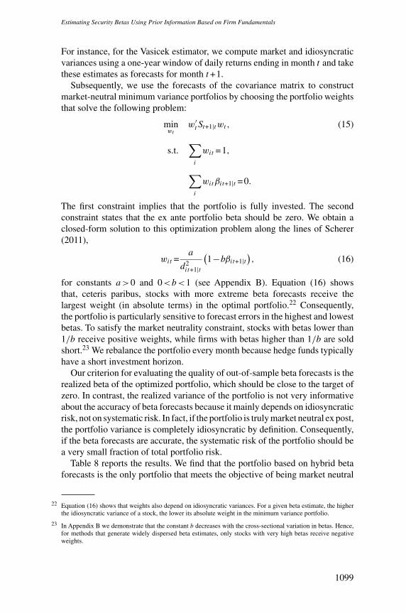
Estimating Security Betas Using Prior Information Based on Firm Fundamentals
For instance, for the Vasicek estimator, we compute market and idiosyncraticvariances using a one-year window of daily returns ending in month t and takethese estimates as forecasts for month t +1.
Subsequently, we use the forecasts of the covariance matrix to constructmarket-neutral minimum variance portfolios by choosing the portfolio weightsthat solve the following problem:
minwt
w′t St+1|twt , (15)
s.t.∑i
wit =1,
∑i
witβit+1|t =0.
The first constraint implies that the portfolio is fully invested. The secondconstraint states that the ex ante portfolio beta should be zero. We obtain aclosed-form solution to this optimization problem along the lines of Scherer(2011),
wit =a
d2it+1|t
(1−bβit+1|t
), (16)
for constants a>0 and 0<b<1 (see Appendix B). Equation (16) showsthat, ceteris paribus, stocks with more extreme beta forecasts receive thelargest weight (in absolute terms) in the optimal portfolio.22 Consequently,the portfolio is particularly sensitive to forecast errors in the highest and lowestbetas. To satisfy the market neutrality constraint, stocks with betas lower than1/b receive positive weights, while firms with betas higher than 1/b are soldshort.23 We rebalance the portfolio every month because hedge funds typicallyhave a short investment horizon.
Our criterion for evaluating the quality of out-of-sample beta forecasts is therealized beta of the optimized portfolio, which should be close to the target ofzero. In contrast, the realized variance of the portfolio is not very informativeabout the accuracy of beta forecasts because it mainly depends on idiosyncraticrisk, not on systematic risk. In fact, if the portfolio is truly market neutral ex post,the portfolio variance is completely idiosyncratic by definition. Consequently,if the beta forecasts are accurate, the systematic risk of the portfolio should bea very small fraction of total portfolio risk.
Table 8 reports the results. We find that the portfolio based on hybrid betaforecasts is the only portfolio that meets the objective of being market neutral
22 Equation (16) shows that weights also depend on idiosyncratic variances. For a given beta estimate, the higherthe idiosyncratic variance of a stock, the lower its absolute weight in the minimum variance portfolio.
23 In Appendix B we demonstrate that the constant b decreases with the cross-sectional variation in betas. Hence,for methods that generate widely dispersed beta estimates, only stocks with very high betas receive negativeweights.
1099
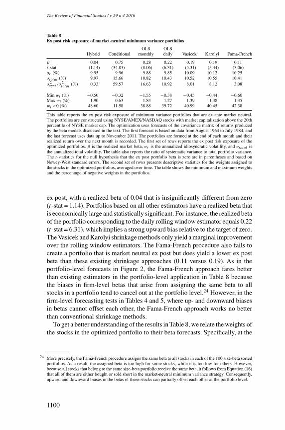
The Review of Financial Studies / v 29 n 4 2016
Table 8Ex post risk exposure of market-neutral minimum variance portfolios
OLS OLSHybrid Conditional monthly daily Vasicek Karolyi Fama-French
β 0.04 0.75 0.28 0.22 0.19 0.19 0.11t-stat (1.14) (34.83) (8.06) (6.31) (5.31) (5.34) (3.06)σε (%) 9.95 9.96 9.88 9.85 10.09 10.12 10.25σtotal (%) 9.97 15.66 10.82 10.43 10.52 10.55 10.41σ2syst /σ
2total
(%) 0.33 59.57 16.63 10.92 8.01 8.12 3.08
Min wi (%) −0.50 −0.32 −1.55 −0.38 −0.45 −0.44 −0.60Max wi (%) 1.90 0.63 1.84 1.27 1.39 1.38 1.35wi <0 (%) 48.60 11.58 38.88 39.72 40.99 40.45 42.38
This table reports the ex post risk exposure of minimum variance portfolios that are ex ante market neutral.The portfolios are constructed using NYSE/AMEX/NASDAQ stocks with market capitalization above the 20thpercentile of NYSE market cap. The optimization uses forecasts of the covariance matrix of returns producedby the beta models discussed in the text. The first forecast is based on data from August 1964 to July 1984, andthe last forecast uses data up to November 2011. The portfolios are formed at the end of each month and theirrealized return over the next month is recorded. The first set of rows reports the ex post risk exposure of theoptimized portfolios. β is the realized market beta, σε is the annualized idiosyncratic volatility, and σtotal isthe annualized total volatility. The table also reports the ratio of systematic variance to total portfolio variance.The t-statistics for the null hypothesis that the ex post portfolio beta is zero are in parentheses and based onNewey-West standard errors. The second set of rows presents descriptive statistics for the weights assigned tothe stocks in the optimized portfolios, averaged over time. The table shows the minimum and maximum weightsand the percentage of negative weights in the portfolios.
ex post, with a realized beta of 0.04 that is insignificantly different from zero(t-stat = 1.14). Portfolios based on all other estimators have a realized beta thatis economically large and statistically significant. For instance, the realized betaof the portfolio corresponding to the daily rolling window estimator equals 0.22(t-stat = 6.31), which implies a strong upward bias relative to the target of zero.The Vasicek and Karolyi shrinkage methods only yield a marginal improvementover the rolling window estimators. The Fama-French procedure also fails tocreate a portfolio that is market neutral ex post but does yield a lower ex postbeta than these existing shrinkage approaches (0.11 versus 0.19). As in theportfolio-level forecasts in Figure 2, the Fama-French approach fares betterthan existing estimators in the portfolio-level application in Table 8 becausethe biases in firm-level betas that arise from assigning the same beta to allstocks in a portfolio tend to cancel out at the portfolio level.24 However, in thefirm-level forecasting tests in Tables 4 and 5, where up- and downward biasesin betas cannot offset each other, the Fama-French approach works no betterthan conventional shrinkage methods.
To get a better understanding of the results in Table 8, we relate the weights ofthe stocks in the optimized portfolio to their beta forecasts. Specifically, at the
24 More precisely, the Fama-French procedure assigns the same beta to all stocks in each of the 100 size-beta sortedportfolios. As a result, the assigned beta is too high for some stocks, while it is too low for others. However,because all stocks that belong to the same size-beta portfolio receive the same beta, it follows from Equation (16)that all of them are either bought or sold short in the market-neutral minimum variance strategy. Consequently,upward and downward biases in the betas of these stocks can partially offset each other at the portfolio level.
1100
Estimating Security Betas Using Prior Information Based on Firm Fundamentals
end of each month, we form ten portfolios by sorting stocks on their predictedbetas. We then calculate the sum of the minimum variance portfolio weights ofthe stocks in each beta decile. Figure 3 plots the summed minimum varianceweights (black diamonds) and the average forecast error (gray bars) for eachdecile.25 The figure shows that the hybrid method outperforms other estimatorsin the portfolio optimization because it sharply reduces forecast errors forthose stocks that receive most weight, that is, the firms with the highest andlowest ex ante estimates of beta. Consistent with Equation (16), we observethat the minimum variance strategy assigns large positive weights to low-betastocks and takes negative positions in high-beta stocks. Existing beta estimatorsunderestimate the low betas and overestimate the high betas. Consequently,the stocks that are bought have a larger ex post beta than predicted, while thestocks that are sold short have a smaller realized beta than expected. Botheffects contribute to the positive market risk exposure of the overall portfoliosin Table 8.
Table 8 further reports the fraction of total portfolio variance that issystematic. As expected, the realized portfolio variance is mostly idiosyncratic.For the portfolios formed using rolling betas, systematic risk makes up about10.9% (daily OLS) to 16.6% (monthly OLS) of total risk. For the Vasicekand Karolyi estimators, the ratio of systematic to total portfolio variance isapproximately 8%, and for the Fama-French approach, it equals 3.1%. The ratiois lowest (0.3%) for the portfolio created using the hybrid estimator, consistentwith the better predictive ability of the hybrid model.
The second set of rows inTable 8 presents descriptive statistics for the weightsassigned to the stocks in the optimized portfolios. We find that none of the betamodels yield extreme positions. For instance, the lowest weight assigned toa stock in the portfolio based on Vasicek betas is -0.45% and the maximumweight is 1.39%. Hence, the significant market risk exposure of the portfoliosformed using existing beta estimators is not driven by extreme positions in afew individual stocks.
In summary, the results from the portfolio optimization highlight the practicalconsequences of inaccurate beta estimation. A hedge fund manager whoconstructs a portfolio that is ex ante market neutral according to existing betaestimators, may find out ex post that this portfolio has a significant exposure tomarket risk. We show that traditional estimators fail to produce a market-neutralportfolio due to systematic errors in beta forecasts. Because our hybrid estimatorsharply reduces estimation errors in extreme betas, the portfolio constructedbased on covariance forecasts from the hybrid model is the only portfolio thatis market neutral ex post.
25 The plot for the Karolyi approach resembles the plot for the Vasicek estimator and is omitted for brevity.
1101
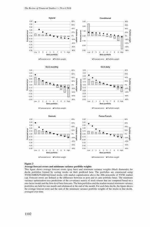
The Review of Financial Studies / v 29 n 4 2016
-80%
-60%
-40%
-20%
0%
20%
40%
60%
80%
-3.00
-2.00
-1.00
0.00
1.00
2.00
3.00
Low 2 3 4 5 6 7 8 9 High
Portfolio weightFo
reca
st e
rror
Beta portfolio
Conditional
Forecast error Portfolio weight
-80%
-60%
-40%
-20%
0%
20%
40%
60%
80%
-0.50
-0.40
-0.30
-0.20
-0.10
0.00
0.10
0.20
0.30
0.40
0.50
Low 2 3 4 5 6 7 8 9 High
Portfolio weightFo
reca
st e
rror
Beta portfolio
OLS daily
Forecast error Portfolio weight
-80%
-60%
-40%
-20%
0%
20%
40%
60%
80%
-0.50
-0.40
-0.30
-0.20
-0.10
0.00
0.10
0.20
0.30
0.40
0.50
Low 2 3 4 5 6 7 8 9 High
Portfolio weightFo
reca
st e
rror
Beta portfolio
Hybrid
Forecast error Portfolio weight
-80%
-60%
-40%
-20%
0%
20%
40%
60%
80%
-0.50
-0.40
-0.30
-0.20
-0.10
0.00
0.10
0.20
0.30
0.40
0.50
Low 2 3 4 5 6 7 8 9 High
Portfolio weightFo
reca
st e
rror
Beta portfolio
OLS monthly
Forecast error Portfolio weight
-80%
-60%
-40%
-20%
0%
20%
40%
60%
80%
-0.50
-0.40
-0.30
-0.20
-0.10
0.00
0.10
0.20
0.30
0.40
0.50
Low 2 3 4 5 6 7 8 9 High
Portfolio weightFo
reca
st e
rror
Beta portfolio
Vasicek
Forecast error Portfolio weight
-80%
-60%
-40%
-20%
0%
20%
40%
60%
80%
-0.50
-0.40
-0.30
-0.20
-0.10
0.00
0.10
0.20
0.30
0.40
0.50
Low 2 3 4 5 6 7 8 9 High
Portfolio weightFo
reca
st e
rror
Beta portfolio
Fama-French
Forecast error Portfolio weight
Figure 3Average forecast errors and minimum variance portfolio weightsThis figure shows average forecast errors (gray bars) and minimum variance weights (black diamonds) fordecile portfolios formed by sorting stocks on their predicted beta. The portfolios are constructed usingNYSE/AMEX/NASDAQ-listed stocks with market capitalization above the 20th percentile of NYSE marketcap. Forecast errors are defined as the difference between ex post and ex ante portfolio betas. The minimumvariance optimization uses predictions of the covariance matrix of stock returns that are computed based on aone-factor model and the firm-level beta forecasts. The beta portfolios and the market-neutral minimum varianceportfolios are held for one month and rebalanced at the end of the month. For each beta decile, the figure showsthe average forecast error and the sum of the minimum variance portfolio weights of the stocks in that decile,averaged over time.
1102
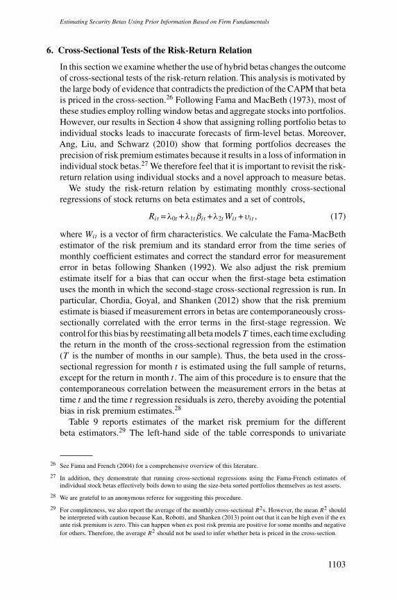
Estimating Security Betas Using Prior Information Based on Firm Fundamentals
6. Cross-Sectional Tests of the Risk-Return Relation
In this section we examine whether the use of hybrid betas changes the outcomeof cross-sectional tests of the risk-return relation. This analysis is motivated bythe large body of evidence that contradicts the prediction of the CAPM that betais priced in the cross-section.26 Following Fama and MacBeth (1973), most ofthese studies employ rolling window betas and aggregate stocks into portfolios.However, our results in Section 4 show that assigning rolling portfolio betas toindividual stocks leads to inaccurate forecasts of firm-level betas. Moreover,Ang, Liu, and Schwarz (2010) show that forming portfolios decreases theprecision of risk premium estimates because it results in a loss of information inindividual stock betas.27 We therefore feel that it is important to revisit the risk-return relation using individual stocks and a novel approach to measure betas.
We study the risk-return relation by estimating monthly cross-sectionalregressions of stock returns on beta estimates and a set of controls,
Rit =λ0t +λ1tβit +λ2tWit +υit , (17)
where Wit is a vector of firm characteristics. We calculate the Fama-MacBethestimator of the risk premium and its standard error from the time series ofmonthly coefficient estimates and correct the standard error for measurementerror in betas following Shanken (1992). We also adjust the risk premiumestimate itself for a bias that can occur when the first-stage beta estimationuses the month in which the second-stage cross-sectional regression is run. Inparticular, Chordia, Goyal, and Shanken (2012) show that the risk premiumestimate is biased if measurement errors in betas are contemporaneously cross-sectionally correlated with the error terms in the first-stage regression. Wecontrol for this bias by reestimating all beta modelsT times, each time excludingthe return in the month of the cross-sectional regression from the estimation(T is the number of months in our sample). Thus, the beta used in the cross-sectional regression for month t is estimated using the full sample of returns,except for the return in month t . The aim of this procedure is to ensure that thecontemporaneous correlation between the measurement errors in the betas attime t and the time t regression residuals is zero, thereby avoiding the potentialbias in risk premium estimates.28
Table 9 reports estimates of the market risk premium for the differentbeta estimators.29 The left-hand side of the table corresponds to univariate
26 See Fama and French (2004) for a comprehensive overview of this literature.
27 In addition, they demonstrate that running cross-sectional regressions using the Fama-French estimates ofindividual stock betas effectively boils down to using the size-beta sorted portfolios themselves as test assets.
28 We are grateful to an anonymous referee for suggesting this procedure.
29 For completeness, we also report the average of the monthly cross-sectional R2s. However, the mean R2 shouldbe interpreted with caution because Kan, Robotti, and Shanken (2013) point out that it can be high even if the exante risk premium is zero. This can happen when ex post risk premia are positive for some months and negativefor others. Therefore, the average R2 should not be used to infer whether beta is priced in the cross-section.
1103
The Review of Financial Studies / v 29 n 4 2016
Table 9Cross-sectional asset pricing tests
No controls With controls
λ0 λ1 Adj. R2 (%) λ0 λ1 Adj. R2 (%)
Hybrid - Bayesian 0.28 0.47 3.61 0.26 0.49 6.76(1.70) (2.08) (1.55) (2.23)
Hybrid - Pooled OLS 0.45 0.28 1.93 0.56 0.23 5.57(2.33) (1.09) (2.90) (0.82)
Hybrid - TS OLS 0.59 0.16 2.99 0.67 0.15 6.16(3.99) (1.01) (4.48) (0.97)
Conditional 0.57 0.15 1.58 0.65 0.13 5.05(4.94) (1.32) (4.88) (1.13)
OLS monthly 0.61 0.11 2.65 0.70 0.08 5.63(4.74) (0.79) (5.00) (0.59)
OLS daily 0.73 0.00 2.98 0.79 0.01 6.04(4.70) (0.04) (5.18) (0.10)
OLS daily - Dimson 0.64 0.10 3.03 0.73 0.06 6.20(4.46) (0.70) (4.83) (0.47)
Vasicek 0.72 0.01 3.00 0.77 0.03 6.45(4.78) (0.11) (5.26) (0.14)
Karolyi 0.72 0.01 3.04 0.76 0.03 6.48(4.76) (0.08) (5.24) (0.13)
Fama-French 0.73 0.00 2.75 0.78 0.03 6.16(4.70) (0.02) (5.32) (0.15)
This table reports Fama-MacBeth estimates for the cross-section of stocks listed on the NYSE, AMEX, andNASDAQ. In the first step, betas are estimated using the procedures described in the text. In the second stage,monthly cross-sectional regressions are run of excess stock returns on the beta estimates and a set of controlvariables to obtain an estimate of the market risk premium λ1:
Rit =λ0t +λ1t βit +λ2tWit +υit ,
whereWit is a vector of control variables that includes the firm characteristics size, book-to-market, momentum,financial leverage, operating leverage, and idiosyncratic volatility. The left-hand side of the table shows estimationresults for cross-sectional regressions without control variables, and the right-hand panel corresponds to cross-sectional regressions with controls. Coefficient estimates are corrected for a contemporaneous EIV bias followingthe procedure described in the text. Shanken-adjusted t-statistics are in parentheses. The reported adjusted R2 isthe average of the monthly cross-sectional adjusted R2s. The sample period is August 1964 to December 2011.
regressions of stock returns on betas. For hybrid betas, we find a positive riskpremium estimate of 0.47% that is statistically significant (t-stat = 2.08) andclose in magnitude to the average excess market return over the sample period(0.42%). In contrast, betas obtained from all other estimators do not carrya significant price of risk. For instance, the risk premium on rolling samplebetas varies from 0.00% per month for one-year daily OLS betas to 0.11% forfive-year monthly OLS betas.
The right-hand panel in Table 9 presents results for Fama-MacBethregressions that include firm characteristics as control variables, motivated bythe conclusion of Fama and French (1992) that beta is no longer priced aftercontrolling for characteristics. We add firm size, book-to-market, momentum,
1104
Estimating Security Betas Using Prior Information Based on Firm Fundamentals
financial leverage, operating leverage, and idiosyncratic volatility to theregressions. Controlling for these characteristics has little impact on theestimates of the market risk premium. In particular, hybrid betas continue tocarry a positive price of risk that is significant at the 5% level. Consistent withprior literature, the risk premium on rolling betas remains insignificant. Aspointed out by Buss and Vilkov (2012), it is hard to detect a significant risk-return relation with rolling betas due to the upward bias in high beta estimatesand downward bias in low betas (see Figure 2). Because of the systematicunderestimation of low betas, returns on low-beta stocks are too high relativeto the predictions of the CAPM, while the returns on high-beta stocks aretoo low due to the overestimation of high betas. As a result, the risk-returnrelation estimated with rolling betas is too flat. In line with Fama and French(1992), we find that assigning portfolio betas to individual stocks also yieldsan insignificant risk premium estimate.
Table 9 further shows that existing shrinkage methods yield littleimprovement over rolling estimators in the cross-sectional tests, even thoughthey improve forecast accuracy. This discrepancy in performance reflectsthe different nature of the forecasting exercise and the asset pricing test.Specifically, the predictability tests in Section 4 are time series tests in which itis crucial that beta estimates are not too extreme. By squaring forecast errors,the MSE criterion penalizes forecasts that are far off target.As a result, methodsthat shrink extreme beta estimates toward a central value (as in Vasicek 1973),and thereby limit the cross-sectional dispersion in betas, tend to do better insuch tests than standard rolling sample estimators. In contrast, in the assetpricing tests cross-sectional variation in betas is needed to capture the observedspread in returns. Hence, assigning a common prior to all firms does not helpin explaining cross-sectional variation in returns.
At first sight, it may seem surprising that the betas estimated using monthlyreturns (conditional betas and five-year rolling betas) yield larger risk premiumestimates than betas computed from daily returns (one-year rolling betas andVasicek and Karolyi betas), even though daily betas tend to be more precise.However, our finding that betas estimated from lower-frequency data carrya higher price of risk than betas estimated from higher-frequency returnsis consistent with prior evidence reported by Handa, Kothari, and Wasley(1989). As pointed out by Kothari, Shanken, and Sloan (1995), one potentialexplanation for the lower risk premium obtained with higher-frequency betasis nonsynchronous trading, which can lead to biased beta estimates. To accountfor this bias, we have estimated Dimson (1979)-corrected daily OLS betas,obtained by adding four lags of the market return to the regression. We findthat this adjustment leads to higher MSEs in the forecasting tests becausethe decrease in the efficiency of beta estimates resulting from the additionallags is larger than the reduction in bias. However, the correction could beimportant for the cross-sectional tests because the bias in daily betas likelyvaries across stocks (a uniform bias does not distort the risk premium estimate).
1105
The Review of Financial Studies / v 29 n 4 2016
Table 9 confirms that correcting daily betas for nonsynchronous trading effectsincreases the risk premium on daily OLS betas, which becomes similar inmagnitude to the premium obtained with monthly OLS betas. Nevertheless,even after the adjustment for nonsynchronous trading, the risk premium onrolling betas remains insignificant.
The beta models that we compare not only differ in terms of data frequencybut also in terms of estimation method. We study the effect of the estimationapproach by comparing the risk premium estimate obtained with full-fledgedhybrid betas to the premium obtained with hybrid specifications in which theprior model is estimated using either time-series or pooled OLS regressionsinstead of Bayesian methods. The results in Table 9 confirm that the estimationmethod plays a crucial role in the asset pricing tests. The model estimatedusing pooled OLS yields an insignificant risk premium of 0.23% per month.Estimating prior betas using a separate time-series regression for each firm alsoyields a risk premium that is too small (0.15%) and statistically insignificant.
These findings highlight a fundamental trade-off in cross-sectional assetpricing tests. On the one hand, we must reduce measurement noise in betasto limit errors-in-variables problems. On the other hand, we need sufficientcross-sectional spread in betas to explain variation in returns. Conventionalbeta estimators fall short on at least one of these dimensions. Conditional betasestimated using time-series regressions exhibit large cross-sectional dispersionbut suffer from large measurement errors. Grouping stocks into portfolios orrunning pooled regressions mitigates noise but leads to a loss of cross-sectionalinformation. Our findings suggest that the hybrid model strikes a better balancebetween reducing noise and preserving information than existing methods.By pooling some coefficients in the prior and leaving other parameters firmspecific, the Bayesian approach not only increases precision but also allowsfor unobserved heterogeneity in betas. As a result, with hybrid betas we find apositive risk-return relation even after controlling for characteristics.
Our goal is not to resurrect the CAPM. Most characteristics in the Fama-MacBeth regressions are significant, in line with the conclusion of Lewellenand Nagel (2006) that a conditional CAPM cannot fully explain anomalieslike the value premium. However, our finding that the market risk premium ispositive and significant for hybrid betas contradicts the common belief in theliterature that beta is dead and provides a strong rationale for the widespreadusage of beta in practice.
7. Conclusion
Firm-specific betas are key inputs for financial decision making but are oftenstrongly time varying and hard to estimate with precision. In this article, wepropose a new approach for estimating individual security betas that improvesprecision by incorporating prior information based on firm fundamentals.Our method is a hybrid of a data-driven rolling sample estimator and the
1106
Estimating Security Betas Using Prior Information Based on Firm Fundamentals
parametric method for modeling beta dynamics proposed by Shanken (1990).The rolling window approach is robust to misspecification of beta dynamics,while the parametric specification is theoretically appealing because it linksbeta to economic state variables and firm fundamentals. Our hybrid procedureexploits the strengths of both methods by combining them in a formal shrinkageframework.
We provide direct evidence on the merits of the hybrid model by predictingbetas out-of-sample. Our results show that the gains of the hybrid estimatorrelative to existing methods are economically large and statistically significant.For instance, MSEs produced by conventional shrinkage estimators are 20%larger at the monthly horizon and more than 50% higher for a five-year periodthan MSEs generated by the hybrid model. The strong outperformance at longhorizons supports our conjecture that incorporating prior knowledge aboutfundamentals can improve beta forecasts because in the long run beta tendstoward a level determined by the fundamentals of the firm.
We quantify the economic benefits of the hybrid beta estimator by examiningits performance in two applications. First, we consider a portfolio manager whoaims to run a market-neutral minimum variance strategy and uses a factor modelto forecast return covariances. We find that the minimum variance portfoliobased on hybrid betas is the only portfolio that is market neutral ex post.Portfolios based on covariance forecasts derived from other estimators havea significantly positive exposure to market risk due to systematic errors inbeta forecasts. Second, we study the impact of hybrid betas on the outcome ofcross-sectional tests of the risk-return relation. We find that hybrid betas yielda market risk premium estimate that is significantly positive and in line withtheoretical predictions, even after controlling for characteristics. In contrast,existing rolling betas, conditional betas, and shrinkage estimates of beta arenot priced in the cross-section.
We identify three key aspects of the hybrid approach that drive its consistentoutperformance. First, shrinkage is more powerful in the hybrid model becausethe prior is unique to each firm and incorporates multiple firm characteristics andeconomic conditioning variables. Other shrinkage methods are less effective incorrecting noisy sample estimates of beta because they employ a common orportfolio-level prior that contains too little economic information. Second, theBayesian approach we use to estimate the fundamentals-based prior increasesprecision by pooling the loadings on the conditioning variables, while alsoallowing for heterogeneity in betas unrelated to fundamentals to mitigatemisspecification bias.Alternative models with firm-level conditioning variablesestimated using standard frequentist methods produce beta forecasts that areeither noisy or biased. Third, the use of mixed frequency data enables us toestimate rolling betas more precisely using daily returns, while at the sametime exploiting prior information embedded in monthly fundamentals.
Our results demonstrate that the method used for measuring beta hasimportant implications, both for academic tests and for practical applications.
1107
The Review of Financial Studies / v 29 n 4 2016
Given these consequences, it is striking that the five-year rolling windowestimator that is widely used in the literature and in practice turns out to be one ofthe worst predictors of beta. We hope that these findings encourage researchersand practitioners to question the routine use of rolling beta estimators andto consider using a better approach for applications that rely on accuratebeta estimates. The hybrid estimator that we propose is useful in many suchapplications. In the paper we demonstrate its benefits for asset pricing tests andportfolio construction, but the approach should also be well suited for cost-of-capital calculations and for computing abnormal returns in event studies.
The hybrid model can be extended in various directions. For instance,the MIDAS approach of Ghysels, Santa-Clara, and Valkanov (2005) can beimplemented to attach optimal weights to the daily returns in the window usedfor estimating rolling sample betas. In addition, methods other than the Bayesianweighting scheme of Vasicek (1973), such as weighting schemes driven by pastforecasting performance, can be used to combine rolling betas and prior betas.30
Furthermore, while we focus on the estimation of market betas because of thewidespread usage of the CAPM, our work can be readily extended to estimatefirm-level betas in multifactor models.
Appendix
A. Prior Distributions for Parameters in the Panel Model
In this Appendix we provide details about the prior distributions that we assume for the parametersin the panel model in Equation (5), which we repeat here for convenience:
Rit =α∗i +(δ0i +δ1iXt−1 +δ′2Zit−1 +δ′3Zit−1Xt−1)RMt +ηit . (A.1)
We stack the firm-specific parameters α∗i , δ0i , and δ1i in the vector θi and the pooled parameters
δ2 and δ3 in the vector ξ . We specify a common prior for the parameters in θi :
θi ∼N (θ ,�θ
). (A.2)
Imposing very sharp priors on the θi parameters by setting the diagonal elements in �θ equal tosmall values is equivalent to pooling the parameters in θi across stocks. Alternatively, specifyingflat priors by setting the diagonal elements in�θ equal to very large values corresponds to runninga separate time-series regression for each firm. Instead, we treat the vector of prior means θ andthe precision matrix �−1
θ as unknown parameters and assume the following uninformative priordensities for these hyperparameters
θ∼N (κ,�κ ), (A.3)
�−1θ ∼W
([ψθSθ ]−1 ,ψθ
), (A.4)
where ψθ and [ψθSθ ]−1 are the degrees of freedom parameter and the scale matrix in the Wishartdistribution W , respectively. We specify an uninformative prior for θ by setting κ equal to the
30 See Timmermann (2006) for a comprehensive survey and discussion of forecast combination schemes andAndreou, Ghysels, and Kourtellos (2013) for a recent application of these methods. Preliminary analyses showthat combination schemes in which weights are inversely proportional to past MSEs do not outperform theweighting scheme of Vasicek (1973). However, more advanced methods to estimate the combination weightsmay do better.
1108

Estimating Security Betas Using Prior Information Based on Firm Fundamentals
zero vector and�κ to 100I , with I denoting the identity matrix. For this flat prior, the conditionalposterior mean of θ reduces to the sample average of all of the θi . We setψθ equal to the dimensionof �θ , because this value gives the lowest possible weight to the prior information (Gelmanet al. 2004). The matrix Sθ is the prior mean of �−1
θ and is set equal to the identity matrix. Thisuninformative prior implies that the conditional posterior mean of the covariance matrix �θ isapproximately equal to the sample variability of the θi around their common mean θ .
For the pooled parameters in ξ , we specify an uninformative prior
ξ∼N (ξ ,�ξ
), (A.5)
with the vector of prior means ξ set equal to zero and the prior covariance matrix �ξ to 100I . Wecomplete the specification of the model by adding a diffuse prior for the idiosyncratic volatilityσηi :
σηi ∝1
σηi. (A.6)
B. Market-Neutral Minimum Variance Portfolios
In this Appendix we solve the optimization problem in Section 5, which can be characterized as
minw
w′Sw, (B.1)
s.t. w′ι=1,
w′β =0,
where w is the N -vector of portfolio weights, S the covariance matrix of stock returns, and β theN -vector of beta forecasts. The constraints can be written in matrix notation as
C′w=c, (B.2)
with C =(ι β) and c=(1 0)′. The general solution to this problem is:
w=S−1C(C′S−1C
)−1c. (B.3)
Assuming a single-factor structure for S and using the matrix inversion lemma, we obtain
S−1 =D−1 − s2
1+s2SββD−1ββ ′D−1, (B.4)
where we define Sgh =g′D−1h for g,h= ι,β. D is a diagonal matrix with idiosyncratic variancesd2i on the main diagonal and s2 is the factor variance. This implies that
S−1C =D−1C
(I− s2
1+s2Sββe2
(β ′D−1C
)), (B.5)
where e2 is a (2×1) vector that selects the second column (i.e., β) from C. The matrix post-multiplication D−1C is of order (2×2). Hence, expression (B.5) shows that the portfolio weightsare in a two-dimensional space spanned by the vectorsD−1C that have elements 1
d2i
and βi
d2i
. That
means the weights can be represented as
wi =a
d2i
(1−bβi ), (B.6)
1109
The Review of Financial Studies / v 29 n 4 2016
with
a=Sββ
SιιSββ−S2ιβ
, (B.7)
b=Sιβ
Sββ. (B.8)
Both the numerator and denominator in (B.7) are positive, and therefore a>0. Under theassumptions that the average beta is one and that βi and 1
d2i
are cross-sectionally independent, for
large N the constant b converges in probability to
E[
1d2
]E [β]
E[
1d2
]E
[β2
] =1
1+ω2β
, (B.9)
where ω2β represents the cross-sectional variance of betas. We therefore find that 0<b<1.
References
Andersen, T., T. Bollerslev, and N. Meddahi. 2005. Correcting the errors: Volatility forecast evaluation usinghigh-frequency data and realized volatilities. Econometrica 73:279–96.
Andersen, T., T. Bollerslev, F. Diebold, and J. Wu. 2000. A framework for exploring the macroeconomicdeterminants of systematic risk. American Economic Review 95:398–404.
———. 2006. Realized beta: Persistence and predictability. In Advances in econometrics: Econometric analysisof economic and financial time series. Eds. T. Fomby and D. Terrell. Amsterdam: Elsevier.
Andreou, E., E. Ghysels, and A. Kourtellos. 2013. Should macroeconomic forecasters use daily financial dataand how? Journal of Business and Economic Statistics 31:240–51.
Ang, A., and J. Chen. 2007. CAPM over the long run: 1926-2001. Journal of Empirical Finance 14:1–40.
Ang, A., J. Liu, and K. Schwarz. 2010. Using stocks or portfolios in tests of factor models. Working Paper,Columbia University.
Avramov, D., and T. Chordia. 2006. Asset pricing models and financial market anomalies. Review of FinancialStudies 19:1001–40.
Berk, J., and J. van Binsbergen. 2016. Assessing asset pricing models using revealed preference. Journal ofFinancial Economics 119:1–23.
Black, F., M. Jensen, and M. Scholes. 1972. The capital asset pricing model: Some empirical tests. In Studies inthe theory of capital markets. Ed. M. Jensen. New York: Praeger.
Bollerslev, T., R. Engle, and J. Wooldridge. 1988. A capital asset pricing model with time-varying covariances.Journal of Political Economy 96:116–31.
Buss, A., and G. Vilkov. 2012. Measuring equity risk with option-implied correlations. Review of FinancialStudies 25:3113–40.
Campbell, J., M. Lettau, B. Malkiel, and Y. Xu. 2001. Have individual stocks become more volatile?An empiricalexploration of idiosyncratic risk. Journal of Finance 56:1–43.
Carlson, M., A. Fisher, and R. Giammarino. 2004. Corporate investment and asset price dynamics: Implicationsfor the cross-section of returns. Journal of Finance 59:2577–603.
Chan, L., J. Karceski, and J. Lakonishok. 1999. On portfolio optimization: Forecasting covariances and choosingthe risk model. Review of Financial Studies 12:937–74.
1110
Estimating Security Betas Using Prior Information Based on Firm Fundamentals
Chordia, T., A. Goyal, and J. Shanken. 2012. Cross-sectional asset pricing with individual stocks: Betas versuscharacteristics. Working Paper, Emory University.
Clark, T., and M. McCracken. 2013. Advances in forecast evaluation. In Handbook of economic forecasting.Eds. G. Elliott and A. Timmermann. Amsterdam: Elsevier.
Diebold, F., and R. Mariano. 1995. Comparing predictive accuracy. Journal of Business and Economic Statistics13:253–63.
Dimson, E. 1979. Risk measurement when shares are subject to infrequent trading. Journal of FinancialEconomics 7:197–226.
Engle, R., E. Ghysels, and B. Sohn. 2013. Stock market volatility and macroeconomic fundamentals. Review ofEconomics and Statistics 95:776–97.
Fama, E., and K. French. 1992. The cross-section of expected stock returns. Journal of Finance 47:427–65.
———. 1997. Industry costs of equity. Journal of Financial Economics 43:153–93.
———. 2004. The capital asset pricing model: Theory and evidence. Journal of Economic Perspectives 18:25–46.
———. 2008. Dissecting anomalies. Journal of Finance 63:1653–78.
Fama, E., and J. MacBeth. 1973. Risk, return and equilibrium: Empirical tests. Journal of Political Economy71:607–36.
Ferson, W., and C. Harvey. 1998. Fundamental determinants of national equity market returns: A perspective onconditional asset pricing. Journal of Banking and Finance 21:1625–65.
———. 1999. Conditioning variables and the cross section of stock returns. Journal of Finance 54:1325–60.
Foster, D., and D. Nelson. 1996. Continuous record asymptotics for rolling sample variance estimators.Econometrica 64:139–74.
Gelman, A., J. Carlin, H. Stern, and D. Rubin. 2004. Bayesian data analysis, 2nd ed. Boca Raton, FL: Chapmanand Hall/CRC.
Ghysels, E., and E. Jacquier. 2007. Market beta dynamics and portfolio efficiency. Working Paper, University ofNorth Carolina and HEC Montreal.
Ghysels, E., P. Santa-Clara, and R. Valkanov. 2005. There is a risk-return trade-off after all. Journal of FinancialEconomics 76:509–48.
Ghysels, E. 1998. On stable factor structures in the pricing of risk: Do time-varying betas help or hurt? Journalof Finance 53:549–73.
Giacomini, R., and H. White. 2006. Tests of conditional predictive ability. Econometrica 74:1545–78.
Gomes, J., L. Kogan, and L. Zhang. 2003. Equilibrium cross-section of returns. Journal of Political Economy111:693–732.
Goyal, A., and I. Welch. 2008. A comprehensive look at the empirical performance of equity premium prediction.Review of Financial Studies 21:1455–508.
Graham, J., and C. Harvey. 2001. Theory and practice of corporate finance: Evidence from the field. Journal ofFinancial Economics 60:187–243.
Grundy, B., and J. Martin. 2001. Understanding the nature of the risks and the source of the rewards to momentuminvesting. Review of Financial Studies 14:29–78.
Gulen, H., Y. Xing, and L. Zhang. 2009. Value versus growth: Time-varying expected stock returns. WorkingPaper, University of Michigan.
Hamada, R. 1972. The effect of the firm’s capital structure on the systematic risk of common stocks. Journal ofFinance 27:435–52.
Handa, P., S. P. Kothari, and C. Wasley. 1989. The relation between the return interval and betas: Implicationsfor the size effect. Journal of Financial Economics 23:79–100.
1111
The Review of Financial Studies / v 29 n 4 2016
Harvey, C. 2001. The specification of conditional expectations. Journal of Empirical Finance 8:573–637.
Harvey, D., S. Leybourne, and P. Newbold. 1997. Testing the equality of prediction mean squared errors.International Journal of Forecasting 13:281–91.
Jagannathan, R., and T. Ma. 2003. Risk reduction in large portfolios: Why imposing the wrong constraints helps.Journal of Finance 58:1651–83.
Jagannathan, R., and Z. Wang. 1996. The conditional CAPM and cross-section of expected returns. Journal ofFinance 51:3–53.
Kan, R., C. Robotti, and J. Shanken. 2013. Pricing model performance and the two-pass cross-sectional regressionmethodology. Journal of Finance 68:2617–49.
Karolyi, A. 1992. Predicting risk: Some new generalizations. Management Science 38:57–74.
Korteweg, A., and M. Sorensen. 2010. Risk and return characteristics of venture capital-backed entrepreneurialcompanies. Review of Financial Studies 23:3738–72.
Kothari, S. P., J. Shanken, and R. Sloan. 1995.Another look at the cross-section of expected stock returns. Journalof Finance 50:185–224.
Ledoit, O., and M. Wolf. 2003. Improved estimation of the covariance matrix of stock returns with an applicationto portfolio selection. Journal of Empirical Finance 10:603–21.
Lewellen, J. 1999. The time-series relations among expected return, risk, and book-to-market. Journal ofFinancial Economics 54:5–43.
Lewellen, J., and S. Nagel. 2006. The conditional CAPM does not explain asset-pricing anomalies. Journal ofFinancial Economics 82:289–314.
Lewellen, J., S. Nagel, and J. Shanken. 2010. A skeptical appraisal of asset pricing tests. Journal of FinancialEconomics 96:175–94.
Livdan, D., H. Sapriza, and L. Zhang. 2009. Financially constrained stock returns. Journal of Finance 64:1827–62.
Newey, W., and K. West. 1987.Asimple, positive semi-definite, heteroskedasticity and autocorrelation consistentcovariance matrix. Econometrica 55:703–8.
Pastor, L., and R. Stambaugh. 1999. Costs of equity capital and model mispricing. Journal of Finance 54:67–121.
Petkova, R., and L. Zhang. 2005. Is value riskier than growth? Journal of Financial Economics 78:187–202.
Scherer, B. 2011. A note on the returns from minimum variance investing. Journal of Empirical Finance 18:652–60.
Shanken, J. 1990. Intertemporal asset pricing: An empirical investigation. Journal of Econometrics 45:99–120.
———. 1992. On the estimation of beta-pricing models. Review of Financial Studies 5:1–34.
Thompson, S. 2011. Simple formulas for standard errors that cluster by both firm and time. Journal of FinancialEconomics 99:1–10.
Timmermann,A. 2006. Forecast combinations. In Handbook of economic forecasting. Eds. G. Elliott, C. Granger,and A. Timmermann. Amsterdam: Elsevier.
Vasicek, O. 1973. A note on using cross-sectional information in Bayesian estimation of security betas. Journalof Finance 28:1233–9.
West, K. 1997. Another heteroskedasticity- and autocorrelation-consistent covariance matrix estimator. Journalof Econometrics 76:171–91.
White, H. 2000. A reality check for data snooping. Econometrica 68:1097–126.
Zhang, L. 2005. The value premium. Journal of Finance 60:67–103.
1112