Embed Size (px)
Citation preview
RATIO-DEPENDENT PREDATOR-PREY MODEL : EFFECTOF ENVIRONMENTAL FLUCTUATION AND STABILITY
M. Bandyopadhyay1 and J. Chattopadhyay2,0
1Department of Mathematics, Scottish Church College, Kolkata - 700006, INDIA
E-mail : malay [email protected] Embryology Research Unit, Indian Statistical Institute, Kolkata - 700108, INDIA
E-mail : [email protected]
Abstract
The present paper deals with a problem of a ratio-dependent predator-prey model.
The deterministic and stochastic behaviour of the model system around biologically
feasible equilibria are studied. Conditions for which the deterministic model enter
into Hopf-bifurcation are worked out. Stochastic stability of the system around posi-
tive interior equilibrium is studied. To substantiate our analytical findings numerical
simulations are carried out for hypothetical set of parameter values.
Key Words : Predator-Prey System, Ratio Dependent, Hopf-bifurcation, White Noise,
Stochastic Stability.
1. Introduction
The dynamical relationship between prey and their predators has long been and willcontinue to be one of the dominant themes in ecology due to its universal existence andimportance [16, 18]. The dynamical problems involved with mathematical modelling ofpredator-prey systems may appear to be simple at first sight, however, the detailed analysisof these model systems often leads to very complicated as well as challenging problems. Themost important part of modelling population ecosystem is to make sure that the concernedmathematical model can exhibit the well known system behaviours for the system underconsideration. Dynamical modelling of ecological systems is frequently an evolving process.A systematic mathematical approach can lead to a better understanding of the plausiblemodels and the exposed discrepancies in turn lead to the necessary modifications [43].
After the pioneering work of Alfred Lotka and Vito Volterra in the middle of 1920 forpredator-prey interactions, prey-dependent predator-prey models were studied extensively[26, 31, 50, 49]. In population dynamics, a functional response of the predator to preydensity refers to the change in the density of prey per unit time per predator as a function ofthe prey density. Quite a good number of works have already been performed in ecologicalsystems [7, 10, 14, 21, 23, 33, 62] where the model systems are based on prey-dependentmodel systems. The classical prey-predator models with prey-dependent functional responsetake the form (or some equivalent form)
dN
dt= rN
(
1 −N
K
)
− p(N)P,dP
dt= cp(N)P − eP (1.1)
where p(N) is the so called prey-dependent functional response (N(t) and P (t) denotes preyand predator population density at any instant of time ‘t’ respectively and other parametershave usual meaning). In most of the cases prey-dependent functional response p(N) isgiven by p(N) = aN/(b + N) or p(N) = aN 2/(b + N 2) or p(N) = aN 2/(b + N + αN 2) orp(N) = aN θ/(b + N θ) or some equivalent form. These type of classical predator-prey modelsystems exhibit not only the well known “paradox of enrichment” formulated by Hairstone
0Corresponding Author
1
et. al. [34] and Rosenzweig [56] but also so-called “biological control paradox”, which wasintroduced by Luck [47]. The “paradox of enrichment” states that enriching a predator-prey system (by increasing the carrying capacity) will cause an increment in equilibriumdensity of predator but not in that of prey population which in turn destabilize the interiorequilibrium. As a result it increases the chance of stochastic extinction of the predatorpopulation. However in nature it is observed that enriching the system increases the prey-density which is not a responsible factor to destabilize a stable equilibrium and fails toincrease the amplitude of oscillations in systems that already cycles [1].
The so called “biological control paradox” states that we cannot have a low and sta-ble prey equilibrium density, which is in contradiction with many examples of successfulbiological controls where the prey population is maintained at low densities compared toits environmental carrying capacity [4, 6]. Further example is, Cactoblastis-Opuntia inAustralia, where the crucial factor seems to be pseudo-interference (see, May [49]), wherebiological control has worked and resulted to low and stable pest densities. So this paradoxis a pure artifact, created by simplifying assumptions on functional response. For the rest,the paradox of enrichment exists, but only in systems where one predator-prey pair existsin isolation and the predictions radically change when they are embedded in a simple foodchain model [52]. Most of the natural systems are indeed more complex where predators be-ing exposed to various degrees of facultative secondary carnivory and interacting with manyother subsystems in various ways. This indicates the fact that the paradox of biologicalcontrol is not intrinsic for most of the predator-prey systems.
There are some good data on simple as well as fairly isolated predator-prey systems,like Mary Power’s Catfish-alga system in Panamian streams [54] where one can find out aninteresting phenomenon that some increment in the resource for prey population at equi-librium increases the predator density in place of prey abundance. In some predator-preysystems where Holling disc is a reasonable assumption for predator (for example, the weasel-vole system found in boreal Europe, where voles have on hiding place and weasels haveno alternative resources) we observe large amplitude oscillations of population distributionlike carnivore-herbivore systems [52, 53]. According to the “paradox of enrichment” thesetype of large amplitude oscillations are expected in relatively productive areas and in themost reproductive parts of tundra, while voles inhabiting less productive tundra areas arerelatively stable [55]. High amplitude oscillations were basic characteristics in high alpinebarrens where predator’s density is low, but at present time with rodent time trajectoriesindicates the fingerprints of predators [60]. The change in dynamic position of herbivoresalong productivity gradients thus indicates necessity of reasonable alteration or correctionsof simple as well as traditional food chain models [52]. Recently, predator-prey models withprey-dependent response function have been facing a great challenge from biological andphysiological researchers [3, 4, 5, 32]. At present time it is clear that predator abundancealso have ability to influence the functional response. Arditi and Ginzburg [5] have suggestedthat, in situations characterized by strong space and time heterogeneities, the functional re-sponse can be approximated by a function of the prey-to-predator ratio. Several biologistsare able to establish the fact that functional responses over typical ecological timescalesought to depend on the densities of both prey and predators, especially when predators haveto search for food and therefore have to share or compete for food. Actually prey-dependentand ratio-dependent models are extremes or limiting cases; prey-dependent models are basedon the daily energy balance of predators on the other hand ratio-dependent models presup-posing that prey are easy to find and that predator dynamics are, in essence, governed bydirect density dependence, with prey densities determining the sizes of defended territories.Within natural environment both aspects have ability to influence predator-prey dynamics,and the issue which of the two extremes is closer to reality in which system is wide open.Moreover, pursuit of prey-dependent approach has proved more fertile since its ‘paradoxes’seem to be quite realistic where the premises for their existence is found, but here opinions
2
may differ and there is no strong evidence to close one door or another.Arditi and Ginzburg [5] first proposed the following Michaelis-Menten-Holling type, ratio-
dependent predator-prey system
dN
dt= rN
(
1 −N
K
)
−αNP
k1P + N,
dP
dt=
cαNP
k1P + N− eP (1.2)
The dynamics of this type of ratio-dependent predator-prey models has been studied bymany researchers (see for example Kuang and Beretta [44]; Jost et. al., [39]; Hsu et. al.,[38]).
Major parts of the work in this direction are based on deterministic models of differen-tial and difference equations. The deterministic approach has, however, some limitationsin biology, it is always difficult to predict especially the future of the system accurately.Deterministic models in ecology do not usually incorporate environmental fluctuation basedupon the idea that in case of large populations, stochastic deviations (or effect of randomenvironmental fluctuation) are small enough to be ignored. Stochastic model provides a morerealistic picture of a natural system than its deterministic counterpart. A central obstaclein the stochastic modelling of an ecosystem is the lack of mathematical machinery availableto analyze non-linear multi-dimensional stochastic models [28, 40, 41]. A quantum leap inthe mathematical sophistication of ecological modelling occurred when May [49] introducedstochastic differential equations to investigate limits to niche overlap in randomly fluctuatingenvironment. Well-known deterministic population models (such as Lotka-Volterra model,Gause type prey-predator model etc.) are the starting points of stochastic multi-speciesmodels which include demographic or environmental stochasticity. The resulting stochasticmodels involve non-linear stochastic differential equations whose solutions pose great diffi-culties. Different techniques of linearization of non-linear stochastic differential equationsgiving rise to a set of deterministic moment equations have been receiving a great deal ofattention in different fields of science and technology [8, 11, 12, 28, 40, 41, 57].
The main object of this paper is to consider a ratio-dependent predator-prey model andits stability behaviours around different equilibrium points with special emphasis on thecontroversial equilibrium point (0, 0) for the ratio-dependent model. Our next objectiveis to develop a stochastic dynamic model for ratio-dependent predator-prey model and toexamine the stability of the model system under random environmental fluctuation. We makea comparative analysis of stability of the model system within deterministic and stochasticenvironment.
2. Deterministic Model
The classical model for predator-prey systems can be written in its classical form by asystem of first order nonlinear ordinary differential equations as
dN
dt= Nf(N) − g(N,P )P,
dP
dt= h(N,P )P − γP (2.1)
with prey abundance N(t) and predator abundance P (t) at any instant of time ‘t’. f(N)is the per capita rate of increase of the prey in absence of predation and ‘γ’ is the food-independent mortality rate of predator, assumed to be constant. Amount of prey biomassconsumed by per predator per unit of time is described by the function g(N,P ), whileh(N,P ) describes per capita production rate of predator. There are a considerable amountof evidence that predator production rate can be modelled as simply proportional to foodintake (up to a very good approximation)
h(N,P ) = eg(N,P ) (2.2)
3
where the constant ‘e’ is interpreted as conversion efficiency and satisfy the condition 0 <e < 1. Specific examples are given by Slobodkin [58] for hydras, by Beddington et. al. [13]for numerous arthropods, and by Coe et. al. [24] for large African herbivores in support ofprevious assumption. The trophic function g(N,P ) is the sole link between prey-predatordynamics [5]. In this paper we will consider the usual logistic form of growth function forprey in absence of predator as
f(N) = r
(
1 −N
K
)
where ‘r’ is the intrinsic growth rate of prey and ‘K’ is the environmental carrying capacity.For the traditional prey-dependent predator-prey models (e.g. (1.1)), the functional responseg(N,P ) depends upon the density of prey population ‘N ’ only as we have remarked inintroduction of this literature. According to Berryman [18], credible and consistent predator-prey model must be able to satisfy the minimum biological property that ‘when resources arelow relative to population density, the predator per-capita growth rate should decline withits density’. However, the prey-dependent predator-prey models are unable to satisfy thiscriteria due to the fact that the predator per-capita growth rate becomes a function of preypopulation ‘N ’ only, which is independent of the density of predators ‘P ’. To overcome thissituation, Arditi and Ginzburg [5] have suggested that for situations characterized by strongspace and time heterogeneities, the functional response can be approximated by a function ofthe prey-(N)-to-predator-(P ) ratio (N/P ) and this leads us to the ratio-dependent functionalresponse g(N,P ) as follows
g := g
(
N
P
)
=α(N/P )
1 + αβ(N/P )=
αN
P + αβN
where ‘α’ represents total attack-rate for predator and ‘β’ is the handling time and thefunctional response is known as Michaelis-Menten-Holling type functional response [39, 43].Under these assumptions the dynamics of ratio-dependent predator-prey system is governedby the following system of first order nonlinear ordinary differential equations
dN
dt= rN
(
1 −N
K
)
−αNP
P + αβN,
dP
dt=
eαNP
P + αβN− γP (2.3)
Initial condition for system of equation (2.2) is given by, N(t = 0) = N0 ≥ 0 and P (t =0) = P0 ≥ 0. It is typical for predator-prey systems positive N−axis, positive P− axisand the interior of the first quadrant are all invariant under system (2.3) and the solutionswith positive initial condition are continues to be positive for all time ‘t’. As observed byFreedman and Mathsen [27], Jost et. al. [39], Kuang and Beretta [44] and Kuang [43],system (2.3) is not well-defined at the origin (0, 0) and hence the model is unable to capturethe idea that the growth rate of both the populations are zero in absence of prey as wellas predator population. To overcome this situation, Xiao and Ruan [63] have modified themodel system (2.3) by redefining it as follows
dN
dt= rN
(
1 −N
K
)
−αNP
P + αβN,
dP
dt=
eαNP
P + αβN− γP when (N,P ) 6= (0, 0) (2.4a)
dN
dt= 0 =
dP
dtwhen (N,P ) = (0, 0) (2.4b)
For sake of simplicity it is convenient to scale the variables as x = N/K, y = P/Kαβ andconsider the dimensionless time τ = tr. The dimensionless equations are
dx
dτ= x(1 − x) −
axy
x + y≡ F1(x, y),
dy
dτ=
bxy
x + y− cy ≡ F2(x, y) (2.5a)
4
F1(0, 0) = F2(0, 0) = 0 (2.5b)
where a = α/r, b = e/βr and c = γ/r. For convenience, in the following, time τ is replacedby t as the dimensionless time. Initial condition for system of equation (2.5) is given by,x(0) = x0 ≥ 0 and y(0) = y0 ≥ 0 which are also biologically meaningful.
2.1 Boundedness
Due to the boundedness of the functional responses, we see that
lim(x,y)→(0,0)
F1(x, y) = lim(x,y)→(0,0)
F2(x, y) = 0
Using equation (2.5b) we can conclude that the functions F1(x, y) and F2(x, y) are continuousfunctions on R
2+ = [(x, y) : x ≥ 0, y ≥ 0]. Straightforward computation shows that they are
Lipschizian on R2+. Hence solution of (2.5) with nonnegative initial condition exists and is
unique. It is also easy to see that these solutions exist for all t > 0 and stay nonnegative. Infact, if x(0) = x0 > 0, then x(t) > 0 for all t > 0. Same argument is true for y-component.Hence, the interior of R
2+ is invariant under model system (2.5). Our next task is to consider
the boundedness for the solutions of the model system (2.5).Lemma 1 : All the solutions of the system (2.5) with the positive initial condition (x0, y0)are uniformly bounded within a region Ω, where,
Ω = (x, y) : 0 ≤ x ≤ 1, 0 ≤ x +a
by ≤
L
c
with L = c + 1/4.Proof : From first equation of (2.5) we get,
dx
dt= x(1 − x) −
axy
x + y≤ x(1 − x)
So, x(t) ≤ 1, as t → +∞.Let us define the function
W (t) = x(t) +a
by(t)
Calculating the time derivative of W (t) along the trajectories of the equations (2.5), we get
d
dtW (t) =
dx
dt+
a
b
dy
dt= x(1 − x) −
ac
by
Clearly, the maximum value of x(1 − x) is 1/4, whenever 0 ≤ x ≤ 1. Then,
d
dtW (t) + cW (t) = x(1 − x) + cx ≤ c +
1
4= L (say)
Thus as t → +∞, 0 ≤ W (t) ≤ L/c [19]. Hence, the system (2.5) is dissipative with theasymptotic bound L/c. This ensures the existence of compact neighborhood Ω which is aproper subset of R2
+ such that for sufficiently large initial conditions (x0, y0) the trajectoriesof the system of equations (2.5) will be always within the set Ω.
Hence we have shown that the model system (2.5) is dissipative.
2.2 Equilibria
For population models in deterministic environments, with the environmental parametersare all well-defined constants, it is a natural curiosity to find out the community equilibriawhere all the species populations have time independent values, that is where all net growthrates are zero. Classical two species predator-prey models always possesses at least three
5
equilibrium points (i) Trivial Equilibrium, (ii) Axial Equilibrium and (iii) Positive InteriorEquilibrium [Kot, 2001]. Earlier works on ratio-dependent predator-prey models (e.g. [27,39, 43, 44]) mentioned that the model system (2.3) cannot be linearized at (0, 0) and con-sistent dynamical analysis for the model system in the vicinity of origin reveals the rich andcomplicated dynamics. Based upon the redefined ratio-dependent predator-prey model (2.4)and its non-dimensionalized version (2.5) we are able to mention that the system of equa-tions (2.5) has two equilibria, one is E0(0, 0) and the other is E1(1, 0) on the x-axis for allpossible as well as admissible values of the parameters involved with the model system (2.5).The third and most interesting equilibrium point (from biological point of view) is E∗(x
∗, y∗)where x∗ and y∗ are non-zero positive solutions of the equations F1(x, y) = 0 = F2(x, y) andis given by
x∗ = 1 − [a(b − c)/b], and y∗ = [(b − c)x∗/c] (2.6)
Simple mathematical argument shows that x∗ is positive for all a < b/(b − c) and positivityof y∗ demands an extra condition b > c.
2.3 Behaviour Around E0(0, 0)
The study of stability plays a significant role to understand the structure and functionsof ecological systems. A variety of ecologically interesting interpretations are involved withthe term “stability”. The most common meaning corresponds to neighborhood stability whichmeans stability in the vicinity of an equilibrium point associated with the deterministic modelsystem. An equilibrium point is called a stable equilibrium point if, when the populationsare perturbed they will return to the equilibrium point with the advancement of time. Thereturn may be achieved either as damped oscillations or monotonically. It is a commonpractice to find out the linearized system of equations around the equilibrium point andthe sign of eigenvalues associated with the corresponding Jacobian matrix determine thestability around the equilibrium point. Before going to study the stability of controversialequilibrium point E0(0, 0) we like to remark that mathematical investigation for the natureof solution for the model system in the vicinity of origin reveals some interesting dynamicalbehaviours depending upon the parametric restrictions. This type of dynamical behaviourhave never been observed in clasical prey-dependent predator-prey models. Based upon theoutcomes of stability analysis around E0(0, 0) one can obtain a clear idea on the possibilityof extinction of either population at low population density of both prey and predators.In case of ratio-dependent predator-prey model it is not possible to linearize the modelsystem around E0(0, 0). To study the behaviour of the model system around E0 we followthe technique developed by Arino et. al. [7]. For rigorous calculation and mathematicaljustification of the said technique, interested readers may consult the work of Arino et. al.[7] and the references therein. For this purpose the model system (2.5) can be written as
dX
dt= H(X(t)) + Q(X(t)) (2.7)
where, H(.) is C1 except at the origin, is continuous and homogeneous function of degreeone, i.e. H(sX) = sH(X) for all scalar s ≥ 0, X(t) = (x1, x2) ∈ R
2+ and Q is a C1 function
and satisfy the condition Q(X) = (X) in the vicinity of origin. The functions H(.) andQ(.) are defined by
H(X) ≡ (H1(X), H2(X)), Q(X) ≡ (Q1(X), Q2(X)) (2.8)
H1(X) = x1 −ax1x2
x1 + x2
, H2(X) =bx1x2
x1 + x2
− cx2 (2.9)
Q1(X) = −x21, Q2(X) = 0 (2.10)
6
Let us assume that X(t) is a solution of (2.7), is bounded such that lim inf t→∞ ‖X(t)‖ = 0.At this situation it is possible to find a sequence X(tn + .) → 0 uniformly as tn → ∞. Define
yn(s) =X(tn + s)
‖X(tn + s)‖(2.11)
Clearly, Yn is a sequence with ‖yn‖ = 1. Applying the Ascoli-Arzela theorem [20], it ispossible to find a subsequence corresponding to yn which converges towards some functiony(t) and the limiting function satisfy the equation
dy
dt= H(y(t)) − (y(t), H(y(t)))y(t) (2.12)
In equation (2.12), (., .) stands for standard inner-product in R2. The steady-states
of (2.12) are vectors V satisfying H(V ) = (V,H(V ))V which are solutions of the nonlineareigenvalue problem, H(V ) = µV with µ = (V,H(V )). These stationary solutions correspondto the fixed directions along which the trajectories of (2.12) may converge asymptotically.Using (2.9), the nonlinear eigenvalue problem becomes
[(1 − µ)v1 + (1 − a)v2]v1, [(b − c)v1 − (c + µ)v2]v2 = 0 (2.13)
Now we are in a position to discuss in detail the possibility to reach the origin following fixeddirections.Case - 1 v1 = 0 and v2 6= 0In this case, there is a possibility to reach origin along y−axis, with µ = −c.Case - 2 v1 6= 0 and v2 = 0In this case, it is possible to reach origin along x−axis, with µ = 1.Case - 3 v1 6= 0 and v2 6= 0In this case, the possibility to reach origin along some fixed direction from the interior offirst quadrant depends upon the existence of real root of the quadratic equation
µ2 + µ(c − 1) + ab − b − bc = 0 (2.14)
The existence of real root of the quadratic equation (2.14) demands
c < b <1
a − 1
[
(c − 1)2
4+ ac
]
(2.15)
Again the upper bound for the parameter b will be biologically feasible if and only if a > 1or equivalently α > r. This result has a biological significance that if the prey-catching capac-ity is higher than the intrinsic growth rate of predator then both the population approachesto total extinction.
Under these three conditions, discussed above, it is possible to reach the trivial equilib-rium point E0(0, 0) and hence E0 is an attractor for the model system (2.5).
2.4 Behaviour Around E1 and E∗
The Jacobian matrix J(x, y) for the system (2.5) at any point of the first quadrant (x, y),except origin, is given by
J(x, y) =
[
−x + axy
(x+y)2− a(x)2
(x+y)2
b(y)2
(x+y)2− bxy
(x+y)2
]
(2.16)
The Jacobian matrix evaluated at the boundary equilibrium point E1(1, 0) takes the form
J1 = [J(x, y)]E1=
[
−1 −a0 b − c
]
(2.17)
7
and therefore, if the positive interior equilibrium point exists (i.e. b > c), E1(1, 0) is alwaysstable along x−direction and unstable along y−direction consequently E1(1, 0) is a saddlepoint.
At the interior equilibrium point E∗(x∗, y∗) Jacobian matrix J∗ is given by
J∗ = [J(x, y)]E∗
=
[
−x∗ + ax∗y∗
(x∗+y∗)2− a(x∗)2
(x∗+y∗)2
b(y∗)2
(x∗+y∗)2− bx∗y∗
(x∗+y∗)2
]
(2.18)
The characteristic equation for the Jacobian matrix J∗ is given by
λ2 + A1λ + A2 = 0, where A1 = −Tr(J∗) and A2 = det(J∗) (2.19)
As det(J∗) = ab(x∗)2y∗/(x∗+y∗)2 > 0 the stability of the equilibrium point E∗ solely dependsupon the sign of Tr(J∗) and hence E∗ is stable if Tr(J∗) < 0 and unstable if Tr(J∗) > 0.It is easy to verify that both the situations are possible for the model system under someappropriate parameter values. In terms of the parameters the stability condition of positiveinterior equilibrium point E∗ is a < b[c + b/(b − c)]/(b + c). We have noted earlier thata < b/(b − c) and b > c are the necessary conditions for the positivity of E∗. Hence thestability of equilibrium point E∗ demands the following condition
a < a ≡ min
[
b
b − c,
b
b + c
(
c +b
b − c
)]
with b > c (2.20)
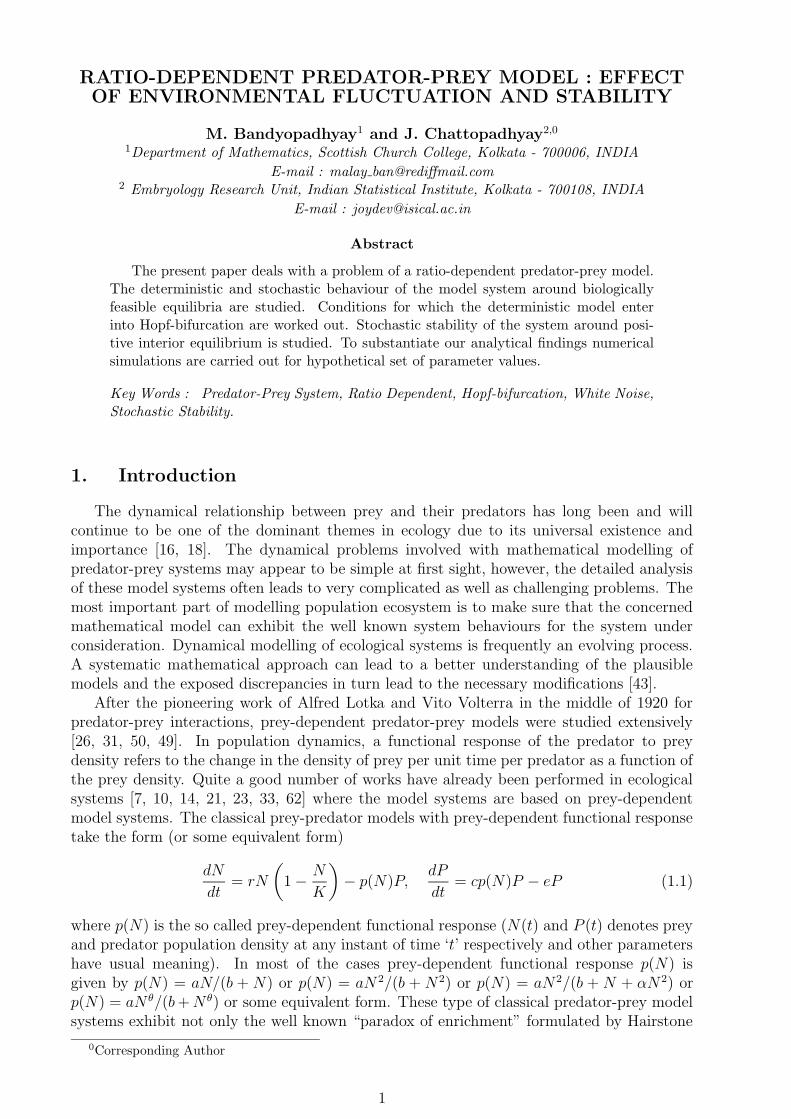
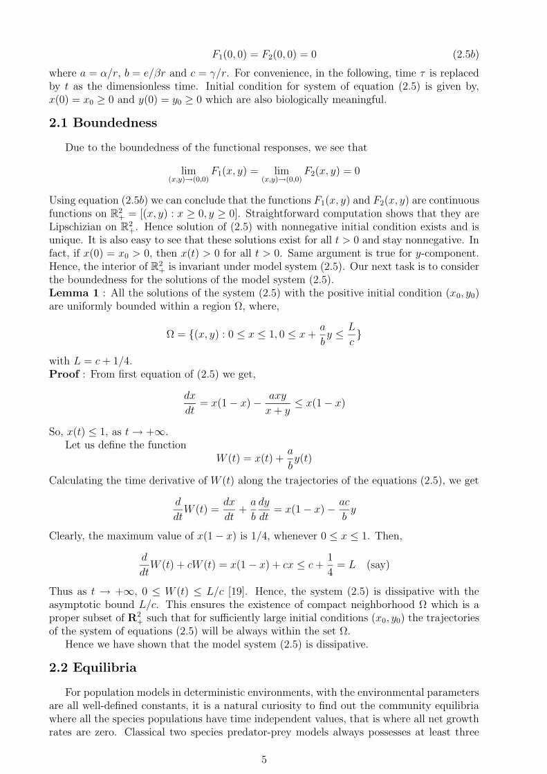
If we increase the value of ‘a’ further such that a > b[c + b/(b − c)]/(b + c) with therestriction b > c then E∗ becomes locally unstable. Hence by the Poincare criteria [11] thereexists at least one limit cycle around E∗ within the positive (x, y)-plane. We now deducethe condition for the existence of a Hopf-bifurcating small amplitude periodic solution.
0 100 200 300 400 500 600 700 800 9000
0.05
0.1
0.15
0.2
0.25
0.3
0.35
0.4
0.45
0.5
Time
Popu
lation
Dist
ribut
ion
Prey Predator
Figure 1: The Hopf-bifurcating periodic solution of the model system (2.5) for parametricvalues a = 2.0, b = 0.7808 and c = 0.5.
Lemma : If a = a∗ = b[c + b/(b − c)]/(b + c) with b > c, then the system (2.5) exhibitHopf-bifurcation near E∗.Proof : At the parametric value a = a∗ = b[c+b/(b−c)]/(b+c), Tr(J∗) = 0 and det(J∗) > 0.When a takes the value a = a∗, the roots of the characteristic equation (2.19) are purely
8
imaginary. Also we can verify the result dda
[Tr(J∗)]a=a∗ 6= 0. Hence both the conditions forHopf-bifurcation [9, 36, 48] are satisfied.
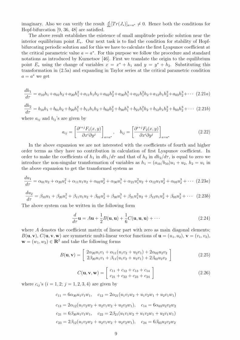
The above result establishes the existence of small amplitude periodic solution near theinterior equilibrium point E∗. Our next task is to find the condition for stability of Hopf-bifurcating periodic solution and for this we have to calculate the first Lyapunov coefficient atthe critical parametric value a = a∗. For this purpose we follow the procedure and standardnotations as introduced by Kuznetsov [46]. First we translate the origin to the equilibriumpoint E∗ using the change of variables x = x∗ + h1 and y = y∗ + h2. Substituting thistransformation in (2.5a) and expanding in Taylor series at the critical parametric conditiona = a∗ we get
dh1
dτ= a10h1+a01h2+a20h
21+a11h1h2+a02h
22+a30h
31+a21h
21h2+a12h1h
22+a03h
32+· · · (2.21a)
dh2
dτ= b10h1 +b01h2 +b20h
21 +b11h1h2 +b02h
22 +b30h
31 +b21h
21h2 +b12h1h
22 +b03h
32 + · · · (2.21b)
where aij and bij’s are given by
aij =
[
∂i+jF1(x, y)
∂xi∂yj
]
a=a∗
, bij =
[
∂i+jF2(x, y)
∂xi∂yj
]
a=a∗
(2.22)
In the above expansion we are not interested with the coefficients of fourth and higherorder terms as they have no contribution in calculation of first Lyapunov coefficient. Inorder to make the coefficients of h1 in dh1/dτ and that of h2 in dh2/dτ , is equal to zero weintroduce the non-singular transformation of variables as h1 = (a10/b10)u1 + u2, h2 = u1 inthe above expansion to get the transformed system as
du1
dτ= α01u2 + α20u
21 + α11u1u2 + α02u
22 + α30u
31 + α21u
21u2 + α12u1u
22 + α03u
32 + · · · (2.23a)
du2
dτ= β10u1 + β20u
21 + β11u1u2 + β02u
22 + β30u
31 + β21u
21u2 + β12u1u
22 + β03u
32 + · · · (2.23b)
The above system can be written in the following form
d
dτu = Au +
1
2B(u,u) +
1
6C(u,u,u) + · · · (2.24)
where A denotes the coefficient matrix of linear part with zero as main diagonal elements;B(u,v), C(u,v,w) are symmetric multi-linear vector functions of u = (u1, u2), v = (v1, v2),w = (w1, w2) ∈ R2 and take the following forms
B(u,v) =
[
2α20u1v1 + α11(u1v2 + u2v1) + 2α02u2v2
2β20u1v1 + β11(u1v2 + u2v1) + 2β02u2v2
]
(2.25)
C(u,v,w) =
[
c11 + c12 + c13 + c14
c21 + c22 + c23 + c24
]
(2.26)
where cij’s (i = 1, 2; j = 1, 2, 3, 4) are given by
c11 = 6α30u1v1w1, c12 = 2α21(u1v1w2 + u1v2w1 + u2v1w1)
c13 = 2α12(u1v2w2 + u2v1w2 + u2v2w1), c14 = 6α03u2v2w2
c21 = 6β30u1v1w1, c22 = 2β21(u1v1w2 + u1v2w1 + u2v1w1)
c23 = 2β12(u1v2w2 + u2v1w2 + u2v2w1), c24 = 6β03u2v2w2
9
Let λ1,2 = ±iω be the eigenvalues of the matrix A and p, q are proper eigenvectors satisfyingthe relations
Aq = iωq, ATp = −iωp, and 〈p,q〉 = 1 (2.27)
where 〈., .〉 means the standard scalar product in C2 : 〈p,q〉 = p1q1 + p2q2. The first
Lyapunov coefficient determining the stability of Hopf-bifurcating periodic solution is givenby [46]
l1 =1
2ω2Re (ig20g11 + ωg21) (2.28)
The quantities g20, g11 and g21 are given by
g20 = 〈p, B(q,q)〉, g11 = 〈p, B(q,q)〉, g21 = 〈p, C(q,q,q)〉 (2.29)
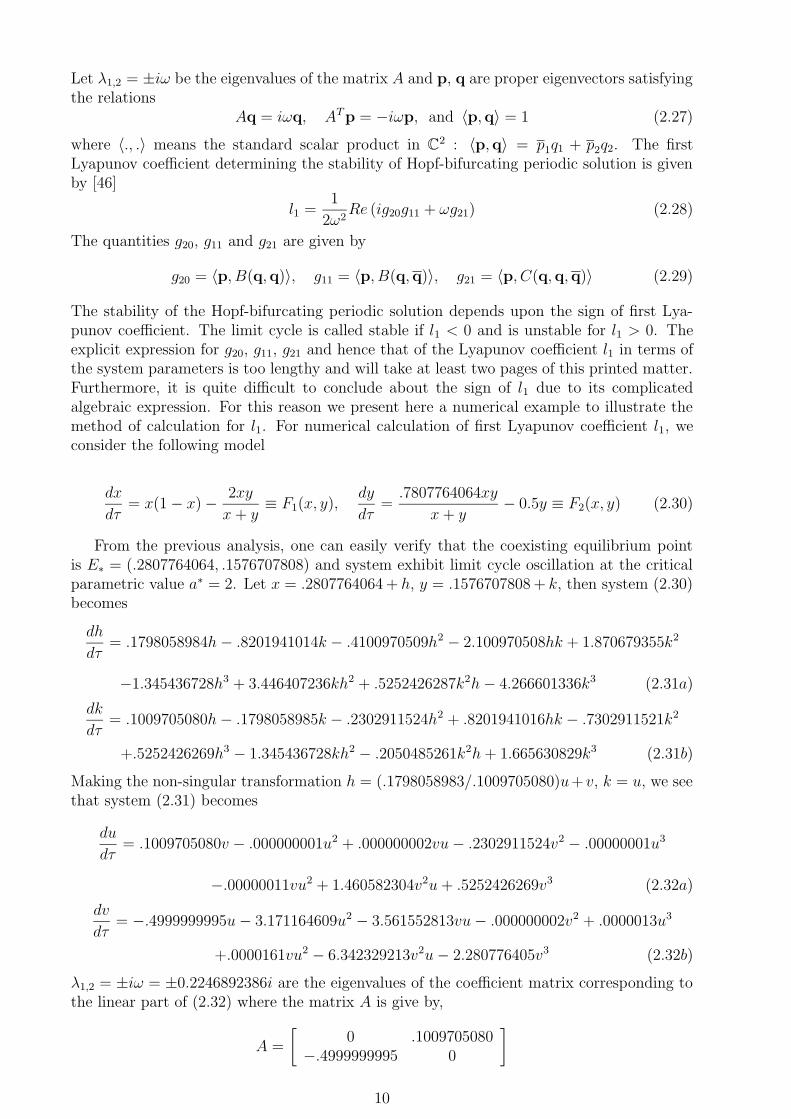
The stability of the Hopf-bifurcating periodic solution depends upon the sign of first Lya-punov coefficient. The limit cycle is called stable if l1 < 0 and is unstable for l1 > 0. Theexplicit expression for g20, g11, g21 and hence that of the Lyapunov coefficient l1 in terms ofthe system parameters is too lengthy and will take at least two pages of this printed matter.Furthermore, it is quite difficult to conclude about the sign of l1 due to its complicatedalgebraic expression. For this reason we present here a numerical example to illustrate themethod of calculation for l1. For numerical calculation of first Lyapunov coefficient l1, weconsider the following model
dx
dτ= x(1 − x) −
2xy
x + y≡ F1(x, y),
dy
dτ=
.7807764064xy
x + y− 0.5y ≡ F2(x, y) (2.30)
From the previous analysis, one can easily verify that the coexisting equilibrium pointis E∗ = (.2807764064, .1576707808) and system exhibit limit cycle oscillation at the criticalparametric value a∗ = 2. Let x = .2807764064 + h, y = .1576707808 + k, then system (2.30)becomes
dh
dτ= .1798058984h − .8201941014k − .4100970509h2 − 2.100970508hk + 1.870679355k2
−1.345436728h3 + 3.446407236kh2 + .5252426287k2h − 4.266601336k3 (2.31a)
dk
dτ= .1009705080h − .1798058985k − .2302911524h2 + .8201941016hk − .7302911521k2
+.5252426269h3 − 1.345436728kh2 − .2050485261k2h + 1.665630829k3 (2.31b)
Making the non-singular transformation h = (.1798058983/.1009705080)u+ v, k = u, we seethat system (2.31) becomes
du
dτ= .1009705080v − .000000001u2 + .000000002vu − .2302911524v2 − .00000001u3
−.00000011vu2 + 1.460582304v2u + .5252426269v3 (2.32a)
dv
dτ= −.4999999995u − 3.171164609u2 − 3.561552813vu − .000000002v2 + .0000013u3
+.0000161vu2 − 6.342329213v2u − 2.280776405v3 (2.32b)
λ1,2 = ±iω = ±0.2246892386i are the eigenvalues of the coefficient matrix corresponding tothe linear part of (2.32) where the matrix A is give by,
A =
[
0 .1009705080−.4999999995 0
]
10
The eigenvectors as defined in (2.27) are given by p = (.1754320563, .07883539039i) andq = (.07883539039, .1754320563i). Now one can calculate the quantities g20, g11, g21 easilyby using any mathematical software (e.g. MAPLE) as
g20 = −.005279657042 + .003107509389i, g11 = .005279657042 + .003107509388i
g21 = −.004581433107 + .005411288533i
Hence the first Lyapunov coefficient l1 is given by
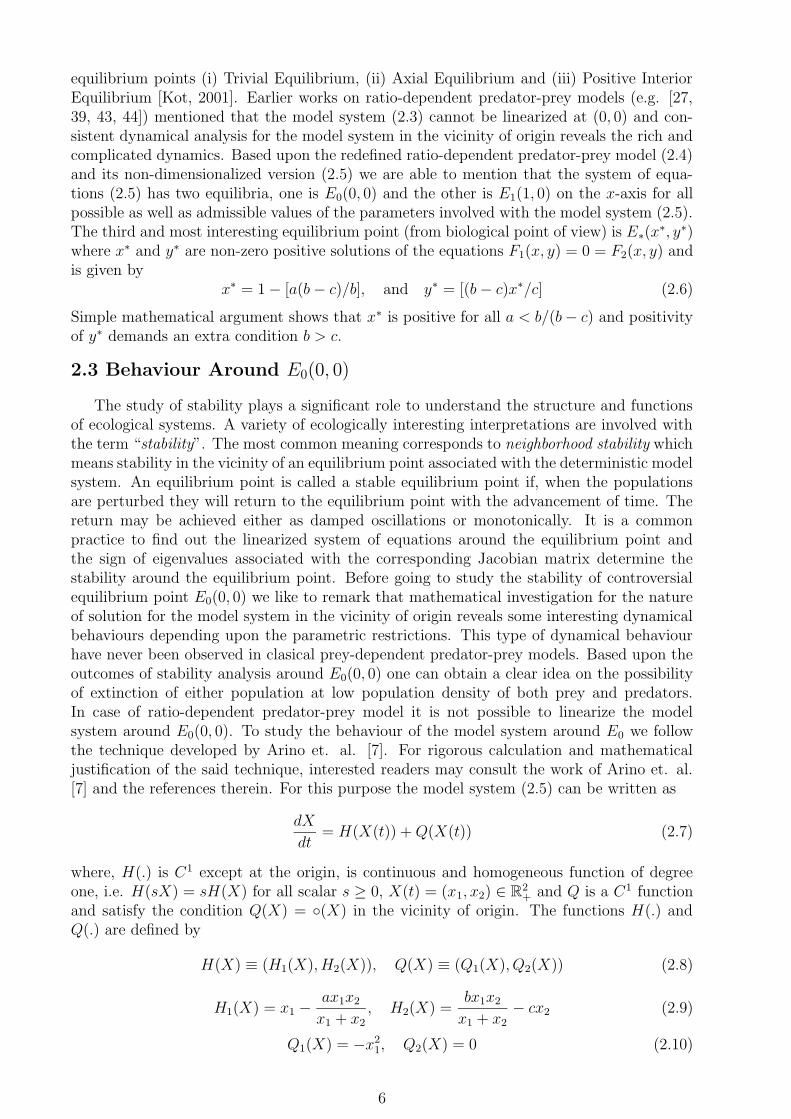
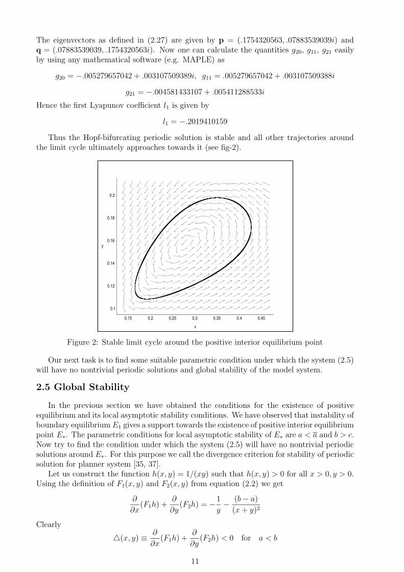
l1 = −.2019410159
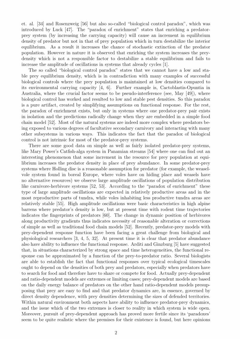
Thus the Hopf-bifurcating periodic solution is stable and all other trajectories aroundthe limit cycle ultimately approaches towards it (see fig-2).
0.1
0.12
0.14
0.16
0.18
0.2
y
0.15 0.2 0.25 0.3 0.35 0.4 0.45
x
Figure 2: Stable limit cycle around the positive interior equilibrium point
Our next task is to find some suitable parametric condition under which the system (2.5)will have no nontrivial periodic solutions and global stability of the model system.
2.5 Global Stability
In the previous section we have obtained the conditions for the existence of positiveequilibrium and its local asymptotic stability conditions. We have observed that instability ofboundary equilibrium E1 gives a support towards the existence of positive interior equilibriumpoint E∗. The parametric conditions for local asymptotic stability of E∗ are a < a and b > c.Now try to find the condition under which the system (2.5) will have no nontrivial periodicsolutions around E∗. For this purpose we call the divergence criterion for stability of periodicsolution for planner system [35, 37].
Let us construct the function h(x, y) = 1/(xy) such that h(x, y) > 0 for all x > 0, y > 0.Using the definition of F1(x, y) and F2(x, y) from equation (2.2) we get
∂
∂x(F1h) +
∂
∂y(F2h) = −
1
y−
(b − a)
(x + y)2
Clearly
4(x, y) ≡∂
∂x(F1h) +
∂
∂y(F2h) < 0 for a < b
11
According to Bendixon-Dulac criterion, there will be no limit cycle in the positive quadrantof xy−plane. Now we can state the following result
Lemma : Existence of interior equilibrium point E∗ along with its local stability and therestriction a < b eliminates the chance of existence of non-trivial periodic solution aroundE∗.
Now we are in a position to prove the global stability of the model system (2.5).
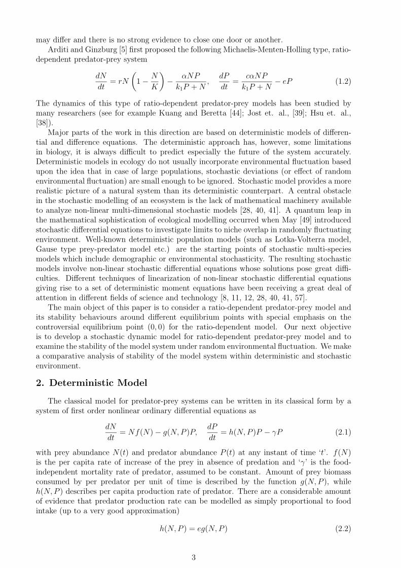
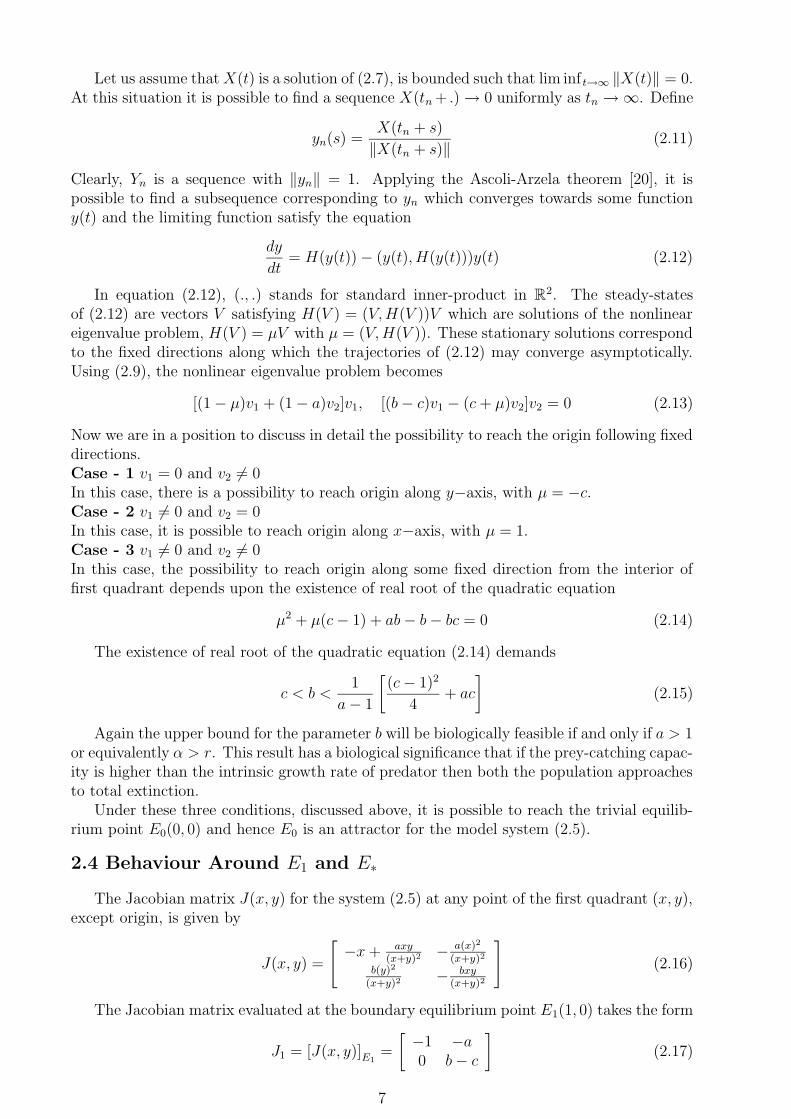
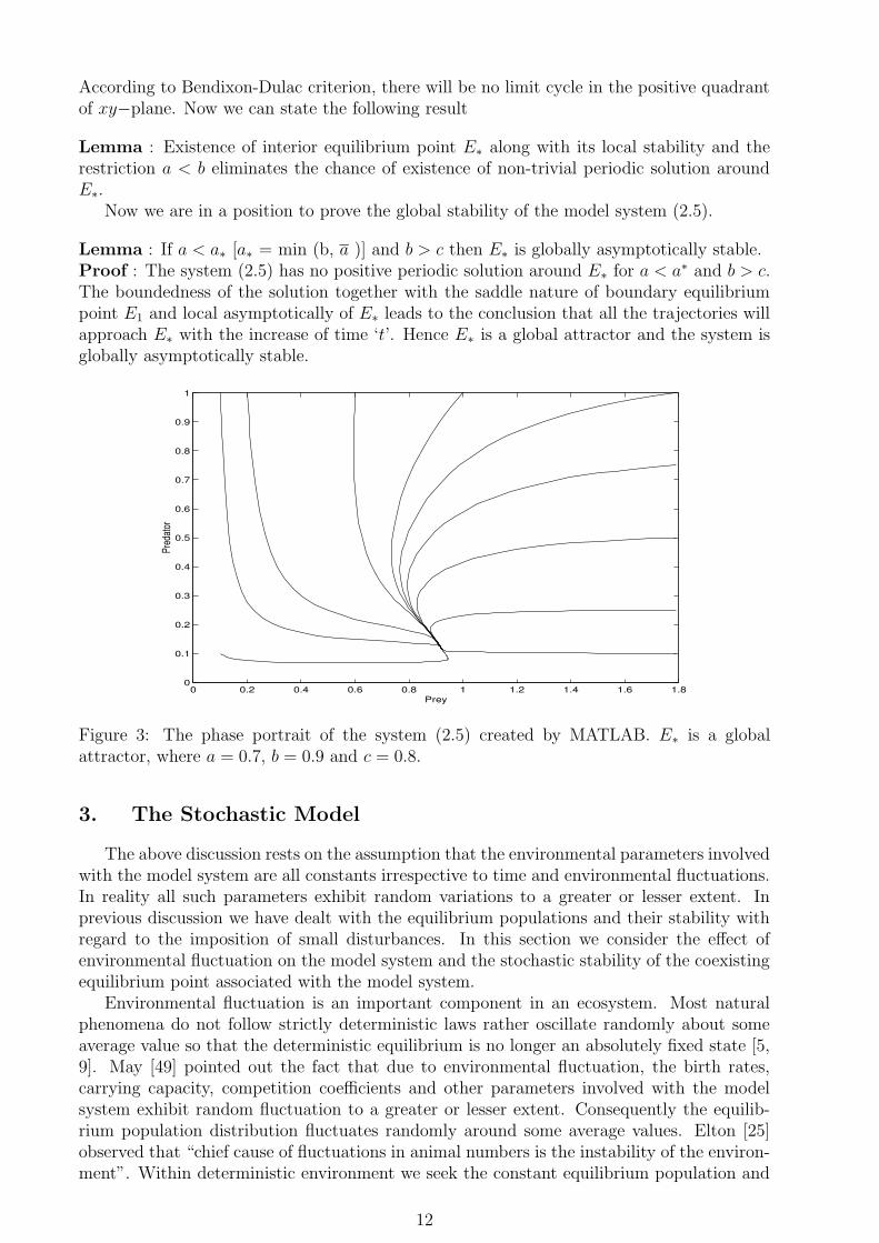
Lemma : If a < a∗ [a∗ = min (b, a )] and b > c then E∗ is globally asymptotically stable.Proof : The system (2.5) has no positive periodic solution around E∗ for a < a∗ and b > c.The boundedness of the solution together with the saddle nature of boundary equilibriumpoint E1 and local asymptotically of E∗ leads to the conclusion that all the trajectories willapproach E∗ with the increase of time ‘t’. Hence E∗ is a global attractor and the system isglobally asymptotically stable.
0 0.2 0.4 0.6 0.8 1 1.2 1.4 1.6 1.80
0.1
0.2
0.3
0.4
0.5
0.6
0.7
0.8
0.9
1
Prey
Pred
ator
Figure 3: The phase portrait of the system (2.5) created by MATLAB. E∗ is a globalattractor, where a = 0.7, b = 0.9 and c = 0.8.
3. The Stochastic Model
The above discussion rests on the assumption that the environmental parameters involvedwith the model system are all constants irrespective to time and environmental fluctuations.In reality all such parameters exhibit random variations to a greater or lesser extent. Inprevious discussion we have dealt with the equilibrium populations and their stability withregard to the imposition of small disturbances. In this section we consider the effect ofenvironmental fluctuation on the model system and the stochastic stability of the coexistingequilibrium point associated with the model system.
Environmental fluctuation is an important component in an ecosystem. Most naturalphenomena do not follow strictly deterministic laws rather oscillate randomly about someaverage value so that the deterministic equilibrium is no longer an absolutely fixed state [5,9]. May [49] pointed out the fact that due to environmental fluctuation, the birth rates,carrying capacity, competition coefficients and other parameters involved with the modelsystem exhibit random fluctuation to a greater or lesser extent. Consequently the equilib-rium population distribution fluctuates randomly around some average values. Elton [25]observed that “chief cause of fluctuations in animal numbers is the instability of the environ-ment”. Within deterministic environment we seek the constant equilibrium population and
12
then investigate their stability which follows from the dynamics of the interactions betweenand within the species. For the systems which are driven by the environmental stochasticity,it is impossible to find a time-independent equilibrium point as a solution of the governingstochastic differential equations. In this situation it is reasonable to find a probabilistic“smoke cloud”, described by the equilibrium probability distribution. For the model sys-tems described by system of stochastic differential equations, there is a continuous spectrumof disturbances generated by the environmental stochasticity, and the system is in tensionbetween two countervailing tendencies. On the one hand, the random environmental fluctua-tions are responsible to spread the cloud, to make the probability distribution move diffusive,while on the other hand, the dynamics of stabilizing population interactions tend to restorethe populations to their mean-value in order to compact the cloud [49]. The model systemswith this type of compact cloud of population distribution is called a stochastically stablesystem. To study the effect of random environmental fluctuation we have to construct thestochastic counter part of the deterministic model system by incorporating environmentalfluctuation.
There are two ways to develop the stochastic model corresponding to an existing de-terministic one to study the effect of fluctuating environment. Firstly, one can replace theenvironmental parameters involved with the deterministic model system by some randomparameters (e.g. the growth rate parameter ‘r’ can be replaced by r0 + εγ(t), where r0 is theaverage growth rate, γ(t) is the noise function and ε is the intensity of fluctuation), secondly,one can add the randomly fluctuating driving force directly to the deterministic growthequations of prey and predator populations without altering any particular parameter [8, 11,59]
Model (2.2) was just a first attempt towards the modelling of predator-prey interac-tion with ratio-dependent functional response. In the present study we introduce stochasticperturbation terms into the growth equations of both prey and predator population to in-corporate the effect of randomly fluctuating environment. We assume that stochastic per-turbations of the state variables around their steady-state values E∗ are of Gaussian whitenoise type which are proportional to the distances of x, y from their steady-state values x∗,y∗ respectively [15]. Gaussian white noise is extremely useful to model rapidly fluctuatingphenomena [11, 59]. So the deterministic model system (2.2) results in following stochasticmodel system
dx = F1(x, y)dt + σ1(x − x∗)dξ1t , dy = F2(x, y)dt + σ2(y − y∗)dξ2
t (3.1)
where σ1, σ2 are real constants and known as intensity of environmental fluctuation, ξ it =
ξi(t), i = 1, 2 are standard Wiener processes independent from each other [30]. In rest of thework we consider (3.1) as an Ito stochastic differential system of the type
dXt = f(t,Xt)dt + g(t,Xt)dξt, Xt0 = X0 (3.2)
where the solution (Xt, t > 0) is a Ito process, ‘f ’ is slowly varying continuous componentor drift coefficient and ‘g’ is the rapidly varying continuous random component or diffusioncoefficient and ξt is a two-dimensional stochastic process having scalar Wiener process com-ponents with increments ∆ξj
t = ξj(t+∆t)−ξj(t) are independent Gaussian random variablesN(0, ∆t). In case of system (3.1),
Xt = (x, y)T , ξt = (ξ1t , ξ
2t )
T , f =
[
F1(x, y)F2(x, y)
]
, g =
[
σ1(x − x∗) 00 σ2(y − y∗)
]
(3.3)
Since the diffusion matrix ‘g’ depends upon the solution Xt, system (3.1) is said to havemultiplicative noise.
3.1 Stochastic Stability of Interior Equilibrium
13
The stochastic differential system (3.1) can be centered at its positive equilibrium pointE∗(x
∗, y∗) by introducing the variables u1 = x − x∗ and u2 = y − y∗. It looks a veryhard problem to derive asymptotic stability in mean square sense by Lyapunov functionsmethod working on the complete nonlinear equations (3.1). For simplicity of mathematicalcalculations we deal with the stochastic differential equations obtained by linearizing thevector function ‘f ’ in (3.3) about the positive equilibrium point E∗. The linearized versionof (3.2) around E∗ is given by
dU(t) = F (U(t))dt + g(U(t))dξ(t) (3.4)
where U(t) = col(u1(t), u2(t)) and
F (U(t)) =
[
−a11u1 − a12u2
a21u1 − a22u2
]
, g(U(t)) =
[
σ1u1 00 σ2u2
]
(3.5)
with
a11 = x∗ −ax∗y∗
(x∗ + y∗)2, a12 =
a(x∗)2
(x∗ + y∗)2, a21 =
b(y∗)2
(x∗ + y∗)2, a22 =
bx∗y∗
(x∗ + y∗)2(3.6)
Note that, in (3.4) the positive equilibrium E∗ corresponds to the trivial solution (u1, u2) =(0, 0). Let Ω be the set defined by Ω = [(t ≥ t0) × R
2, t0 ∈ R+]. Let V ∈ C2(Ω) be a twice
differentiable function of time t. We define the following theorem due to Afanas’ev et. al.[2],
Theorem : Suppose there exists a function V (U, t) ∈ C2(Ω) satisfying the inequalities
K1|U |α ≤ V (U, t) ≤ K2|U |α (3.7)
LV (U, t) ≤ −K3|U |α, Ki > 0, i = 1, 2, 3, α > 0 (3.8)
Then the trivial solution of (3.4) is exponentially α-stable for all time t ≥ 0.
With reference to (3.8) the expression for LV (U, t) is defined by
LV (U, t) =∂V (U, t)
∂t+ F T (U)
∂V (U, t)
∂U+
1
2Tr
[
gT (U)∂2V (U, t)
∂U2g(U)
]
(3.9)
where∂V (U, t)
∂U= col
(
∂V
∂u1
,∂V
∂u2
)
,∂2V (U, t)
∂U2=
[
(
∂2V
∂ui∂uj
)
i,j=1,2
]
(3.10)
Let us consider the Lyapunov function
V (U(t), t) =1
2
[
u21 + ω1u
22
]
(3.11)
where ω1 is a positive real constant to be chosen later. It can be easily checked that (3.7)holds for the Lyapunov function defined in (3.11) with α = 2. Now,
LV (U, t) = (−a11u1 − a12u2)u1 + (a21u1 − a22u2)ω1u2 +1
2Tr
[
gT (U)∂2V (U, t)
∂U2g(U)
]
(3.12)
From (3.5), (3.10) and (3.11) we get,
∂2V
∂u2=
[
1 00 ω1
]
, gT (U)∂2V (U, t)
∂U2g(U) =
[
σ21u
21 0
0 ω1σ22u
22
]
(3.13)
14
Hence from (3.12) we get,
LV (U, t) = −
(
2a11 −σ2
1
2
)
u21 + 2(a21ω1 − a12)u1u2 −
(
2a22 −ω1σ
22
2
)
u22
If we choose ω1 = (a12/a21) > 0, then from above result we get,
LV (U, t) = −
(
2a11 −σ2
1
2
)
u21 −
(
2a22 −a12σ
22
2a21
)
u22 = −UT QU (3.14)
where, Q = diag[(2a11 − σ21/2), (2a22 − a12σ
22/2a21)] and the diagonal matrix Q will be a real
symmetric positive definite matrix and hence its eigenvalues λ1 and λ2 will be positive realquantities if and only if the following conditions hold
σ21 < 4a11 with a11 > 0 and σ2
2 <4a22a21
a12
(3.15)
If λm stands for minimum of two positive eigenvalues λ1 and λ2 for the diagonal matrix Qthen from (3.14) we get the following result
LV (U, t) ≤ −λm|U |2 (3.16)
This leads us to the following result
Theorem : Assume that for some positive real value of ω1 = a12/a21 and the inequalities in(3.15) hold then the zero solution of system (3.4) is asymptotically mean square stable.
Recall that a < a and b > c are the conditions for deterministic stability of the interiorequilibrium point E∗. Conditions for deterministic stability of interior equilibrium pointalong with the inequalities (3.15) are the necessary conditions for stochastic stability ofthe model system under environmental fluctuation. Inequalities (3.15) defines the upperthreshold values for the intensities of the environmental fluctuations ‘σ1’ and ‘σ2’ determinedby the system parameters (i.e. a, b and c) as
σ21 < σ2
1 = 4
[
b2 − a(b − c)2
b2
]
and σ22 < σ2
2 =4(b − c)3
ac(3.17)
Thus the internal parameters of the model system and the intensities of environmentalfluctuation have ability to maintain the stability of the stochastic model system and exhibit abalanced dynamics at any future time within a bounded domain of (a, b, c, σ1, σ2)−parametricspace. The boundaries of the bounded set in (a, b, c, σ1, σ2)−parametric space is defined bythe following inequalities (which are some implicit functional relations)
a < a, b > c, σ21 < σ2
1, σ22 < σ2
2 (3.18)
where the expressions for a, σ21 and σ2
2 are given in (2.20) and (3.17) respectively. Theinequalities in (3.17) can be put into an alternative form as
a <
[
b
b − c
]2 [
1 −σ2
1
4
]
and a <4(b − c)3
cσ22
(3.19)
For a given set of values for b, c, σ1 and σ2 with b > c we can find an estimate for theparameter ‘a’ which will ensure the deterministic stability as well as stochastic stability ofinterior equilibrium point E∗ for the model system (2.5). Defining the upper threshold limit‘a’ for ‘a’ as
A = min
[
b
b − c,
b
b + c
(
c +b
b − c
)
,
[
b
b − c
]2 [
1 −σ2
1
4
]
,4(b − c)3
cσ22
]
(3.20)
15
we can conclude that a < A and b > c are the necessary and sufficient conditions for thestochastic stability of interior equilibrium point E∗ for the model system under consideration.
3.2 Numerical Simulation
In order to give some support to the stability results of the stochastic model systemobtained in the previous section, we numerically simulate the solution of the stochastic dif-ferential equation (SDE) (3.1). For this purpose we have to keep in mind that approximatedsample paths or trajectories of Ito processes obtained from direct simulation must be closeto those of the original Ito process and these will lead us to the concept of strong solutionfor a system of stochastic differential equation [21]. To find the approximate strong solutionof Ito system of SDE’s (3.1) with given initial condition we use the Euler-Maruyama (EM)and Milstein method.
Consider the discretization of the time interval [t0, tf ] with
t0 = 0 < t1 < t2 < · · · < tn < · · · < tN < tN+1 = tf
and the simplest stochastic numerical scheme for the system under consideration is the EM- method
uk,n+1 = uk,n + f(tn, uk,n)4tn + g(tn, uk,n)4ξkn
with uk,0 = uk0, k = 1, 2 and un = [u1,n, u2,n] is the numerical solution at time ‘tn’. In abovenumerical scheme, the increments are given by
4tn = tn+1 − tn
4ξkn = ξk
n+1 − ξkn = ξk(tn+1) − ξk(tn)
where n = 0, 1, 2, ..., NThe noise increments 4ξk
n are N(0,4tn)-distributed independent random variables whichcan be generated numerically by pseudo-random number generators.
An efficient way to evaluate the increments of the Wiener process 4ξkn is to consider
4ξkn =
√
Ink4tn
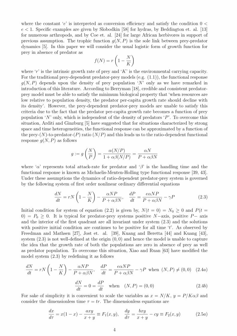
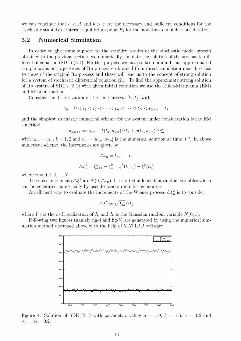
where Ink is the n-th realization of Ik and Ik is the Gaussian random variable N(0, 1).Following two figures (namely fig-4 and fig-5) are generated by using the numerical sim-
ulation method discussed above with the help of MATLAB software.
100 200 300 400 500 600 700 800 9000
0.1
0.2
0.3
0.4
0.5
0.6
0.7
0.8Prey Predator
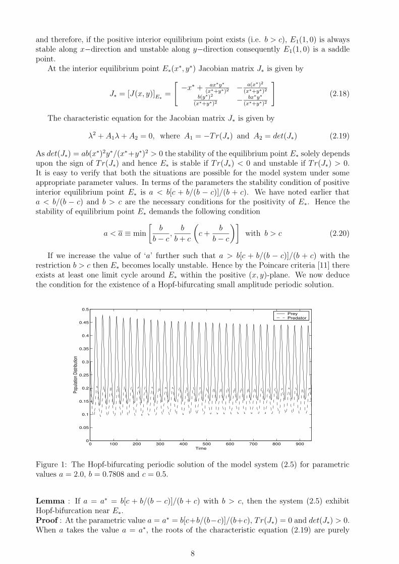
Figure 4: Solution of SDE (3.1) with parametric values a = 1.9, b = 1.5, c = 1.2 andσ1 = σ2 = 0.2.
16
0.59 0.6 0.61 0.62 0.63 0.64 0.650.14
0.145
0.15
0.155
0.16
0.165
0.17
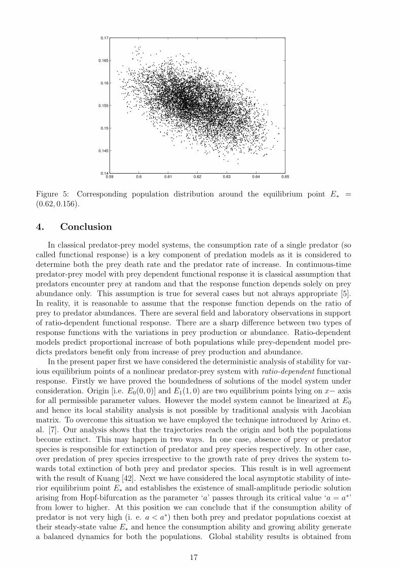
Figure 5: Corresponding population distribution around the equilibrium point E∗ =(0.62, 0.156).
4. Conclusion
In classical predator-prey model systems, the consumption rate of a single predator (socalled functional response) is a key component of predation models as it is considered todetermine both the prey death rate and the predator rate of increase. In continuous-timepredator-prey model with prey dependent functional response it is classical assumption thatpredators encounter prey at random and that the response function depends solely on preyabundance only. This assumption is true for several cases but not always appropriate [5].In reality, it is reasonable to assume that the response function depends on the ratio ofprey to predator abundances. There are several field and laboratory observations in supportof ratio-dependent functional response. There are a sharp difference between two types ofresponse functions with the variations in prey production or abundance. Ratio-dependentmodels predict proportional increase of both populations while prey-dependent model pre-dicts predators benefit only from increase of prey production and abundance.
In the present paper first we have considered the deterministic analysis of stability for var-ious equilibrium points of a nonlinear predator-prey system with ratio-dependent functionalresponse. Firstly we have proved the boundedness of solutions of the model system underconsideration. Origin [i.e. E0(0, 0)] and E1(1, 0) are two equilibrium points lying on x− axisfor all permissible parameter values. However the model system cannot be linearized at E0
and hence its local stability analysis is not possible by traditional analysis with Jacobianmatrix. To overcome this situation we have employed the technique introduced by Arino et.al. [7]. Our analysis shows that the trajectories reach the origin and both the populationsbecome extinct. This may happen in two ways. In one case, absence of prey or predatorspecies is responsible for extinction of predator and prey species respectively. In other case,over predation of prey species irrespective to the growth rate of prey drives the system to-wards total extinction of both prey and predator species. This result is in well agreementwith the result of Kuang [42]. Next we have considered the local asymptotic stability of inte-rior equilibrium point E∗ and establishes the existence of small-amplitude periodic solutionarising from Hopf-bifurcation as the parameter ‘a’ passes through its critical value ‘a = a∗’from lower to higher. At this position we can conclude that if the consumption ability ofpredator is not very high (i. e. a < a∗) then both prey and predator populations coexist attheir steady-state value E∗ and hence the consumption ability and growing ability generatea balanced dynamics for both the populations. Global stability results is obtained from
17
the condition for non-existence of trivial periodic solution around E∗ with the parametricrestrictions obtained in the last part of section 2.
On the other hand for the stochastic version of the model system we have obtained thecondition for asymptotic stability of equilibrium point E∗ in mean square sense by using asuitable Lyapunov function (3.11). These conditions depend upon σ1, σ2 and the parametersinvolved with the model system. For the deterministic environment, the stability of equilib-rium point demands that all eigenvalues of the Jacobian matrix will lie in the left-hand halfof the complex plane. For the corresponding model within stochastic environment, this con-dition is necessary, but insufficient, due to the existence of a relatively compact equilibriumprobability cloud for the populations around deterministic equilibrium point. The stochasticstability requires that the stability provided by the interactions (which is measured by thereal parts of eigenvalues of Jacobian matrix) be sufficient to counteract the driving arisingout from random environmental fluctuations [49]. Regarding stability and instability of thestochastic model system, it intuitively seems appropriate to refer the systems characterizedby large fluctuations in the population numbers as “unstable” and to those with relativelysmall fluctuations as “stable”. For stochastic model system (3.1) asymptotic stability of E∗
in mean square sense depends upon the restriction (3.15). Recall that the feasible values ofthe intensities of environmental fluctuations depend on the system parameters and which inturn decreases with the increase of the parameter ‘a’. For a given set of values of a, b andc one can easily calculate the upper bounds σ2
1 and σ22 from the relation (3.17). Within the
natural environment it is not possible to control the surroundings in such a way that theintensities of environmental fluctuations can not exceed the upper bounds settled for themby the system parameters. The restrictions (3.15) or equivalently (3.17) are the boundariesdetermined by the mathematical methods to obtain a stable population distribution aroundthe equilibrium point within a fluctuating environment. Hence we conclude that to preservethe system stochastically stable the above restriction should be maintained.
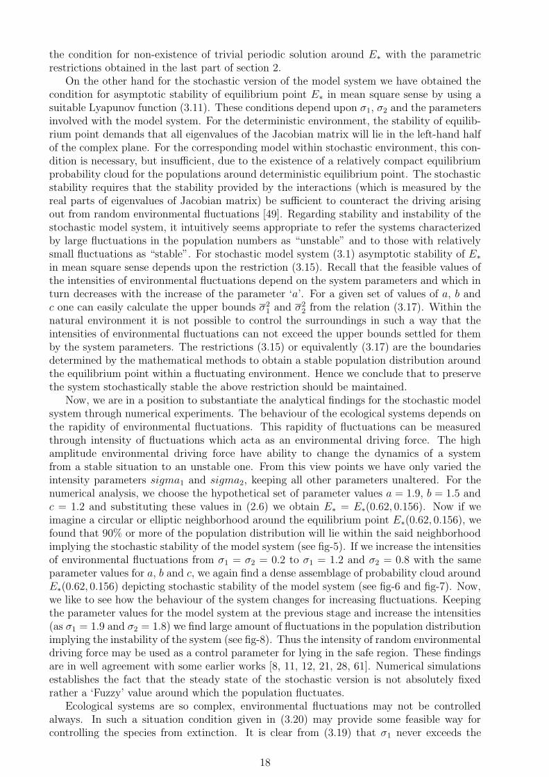
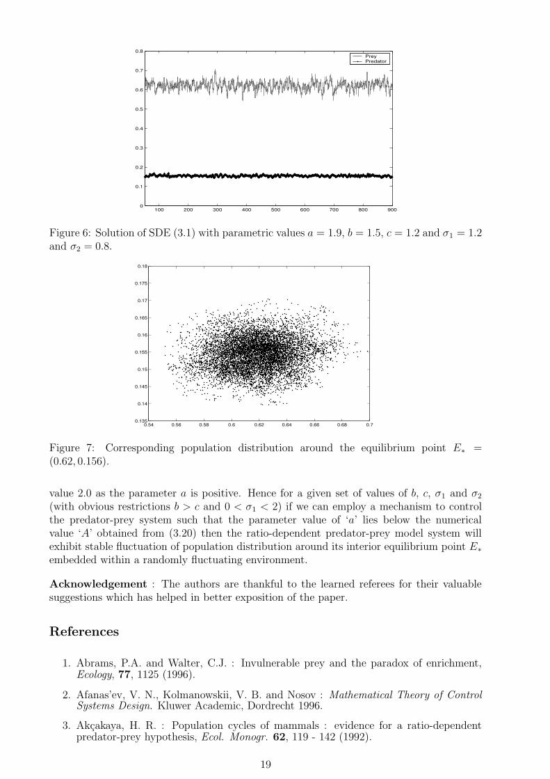
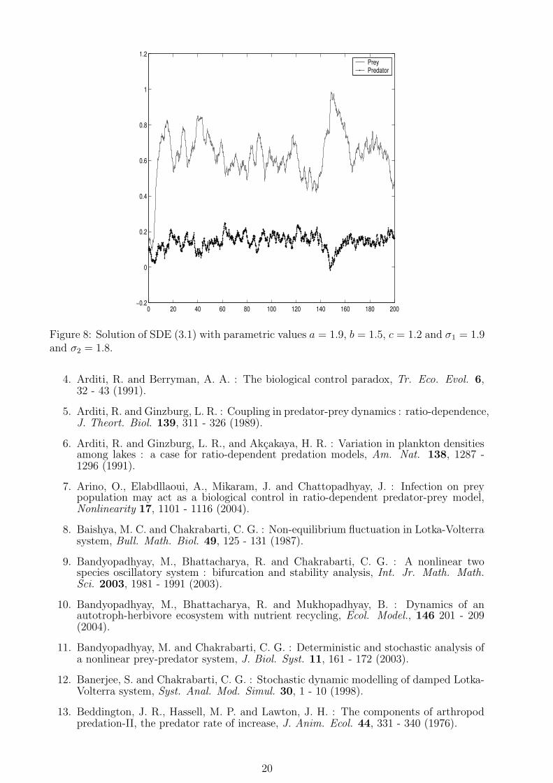
Now, we are in a position to substantiate the analytical findings for the stochastic modelsystem through numerical experiments. The behaviour of the ecological systems depends onthe rapidity of environmental fluctuations. This rapidity of fluctuations can be measuredthrough intensity of fluctuations which acta as an environmental driving force. The highamplitude environmental driving force have ability to change the dynamics of a systemfrom a stable situation to an unstable one. From this view points we have only varied theintensity parameters sigma1 and sigma2, keeping all other parameters unaltered. For thenumerical analysis, we choose the hypothetical set of parameter values a = 1.9, b = 1.5 andc = 1.2 and substituting these values in (2.6) we obtain E∗ = E∗(0.62, 0.156). Now if weimagine a circular or elliptic neighborhood around the equilibrium point E∗(0.62, 0.156), wefound that 90% or more of the population distribution will lie within the said neighborhoodimplying the stochastic stability of the model system (see fig-5). If we increase the intensitiesof environmental fluctuations from σ1 = σ2 = 0.2 to σ1 = 1.2 and σ2 = 0.8 with the sameparameter values for a, b and c, we again find a dense assemblage of probability cloud aroundE∗(0.62, 0.156) depicting stochastic stability of the model system (see fig-6 and fig-7). Now,we like to see how the behaviour of the system changes for increasing fluctuations. Keepingthe parameter values for the model system at the previous stage and increase the intensities(as σ1 = 1.9 and σ2 = 1.8) we find large amount of fluctuations in the population distributionimplying the instability of the system (see fig-8). Thus the intensity of random environmentaldriving force may be used as a control parameter for lying in the safe region. These findingsare in well agreement with some earlier works [8, 11, 12, 21, 28, 61]. Numerical simulationsestablishes the fact that the steady state of the stochastic version is not absolutely fixedrather a ‘Fuzzy’ value around which the population fluctuates.
Ecological systems are so complex, environmental fluctuations may not be controlledalways. In such a situation condition given in (3.20) may provide some feasible way forcontrolling the species from extinction. It is clear from (3.19) that σ1 never exceeds the
18
100 200 300 400 500 600 700 800 9000
0.1
0.2
0.3
0.4
0.5
0.6
0.7
0.8Prey Predator
Figure 6: Solution of SDE (3.1) with parametric values a = 1.9, b = 1.5, c = 1.2 and σ1 = 1.2and σ2 = 0.8.
0.54 0.56 0.58 0.6 0.62 0.64 0.66 0.68 0.70.135
0.14
0.145
0.15
0.155
0.16
0.165
0.17
0.175
0.18
Figure 7: Corresponding population distribution around the equilibrium point E∗ =(0.62, 0.156).
value 2.0 as the parameter a is positive. Hence for a given set of values of b, c, σ1 and σ2
(with obvious restrictions b > c and 0 < σ1 < 2) if we can employ a mechanism to controlthe predator-prey system such that the parameter value of ‘a’ lies below the numericalvalue ‘A’ obtained from (3.20) then the ratio-dependent predator-prey model system willexhibit stable fluctuation of population distribution around its interior equilibrium point E∗
embedded within a randomly fluctuating environment.
Acknowledgement : The authors are thankful to the learned referees for their valuablesuggestions which has helped in better exposition of the paper.
References
1. Abrams, P.A. and Walter, C.J. : Invulnerable prey and the paradox of enrichment,Ecology, 77, 1125 (1996).
2. Afanas’ev, V. N., Kolmanowskii, V. B. and Nosov : Mathematical Theory of ControlSystems Design. Kluwer Academic, Dordrecht 1996.
3. Akcakaya, H. R. : Population cycles of mammals : evidence for a ratio-dependentpredator-prey hypothesis, Ecol. Monogr. 62, 119 - 142 (1992).
19
0 20 40 60 80 100 120 140 160 180 200−0.2
0
0.2
0.4
0.6
0.8
1
1.2Prey Predator
Figure 8: Solution of SDE (3.1) with parametric values a = 1.9, b = 1.5, c = 1.2 and σ1 = 1.9and σ2 = 1.8.
4. Arditi, R. and Berryman, A. A. : The biological control paradox, Tr. Eco. Evol. 6,32 - 43 (1991).
5. Arditi, R. and Ginzburg, L. R. : Coupling in predator-prey dynamics : ratio-dependence,J. Theort. Biol. 139, 311 - 326 (1989).
6. Arditi, R. and Ginzburg, L. R., and Akcakaya, H. R. : Variation in plankton densitiesamong lakes : a case for ratio-dependent predation models, Am. Nat. 138, 1287 -1296 (1991).
7. Arino, O., Elabdllaoui, A., Mikaram, J. and Chattopadhyay, J. : Infection on preypopulation may act as a biological control in ratio-dependent predator-prey model,Nonlinearity 17, 1101 - 1116 (2004).
8. Baishya, M. C. and Chakrabarti, C. G. : Non-equilibrium fluctuation in Lotka-Volterrasystem, Bull. Math. Biol. 49, 125 - 131 (1987).
9. Bandyopadhyay, M., Bhattacharya, R. and Chakrabarti, C. G. : A nonlinear twospecies oscillatory system : bifurcation and stability analysis, Int. Jr. Math. Math.Sci. 2003, 1981 - 1991 (2003).
10. Bandyopadhyay, M., Bhattacharya, R. and Mukhopadhyay, B. : Dynamics of anautotroph-herbivore ecosystem with nutrient recycling, Ecol. Model., 146 201 - 209(2004).
11. Bandyopadhyay, M. and Chakrabarti, C. G. : Deterministic and stochastic analysis ofa nonlinear prey-predator system, J. Biol. Syst. 11, 161 - 172 (2003).
12. Banerjee, S. and Chakrabarti, C. G. : Stochastic dynamic modelling of damped Lotka-Volterra system, Syst. Anal. Mod. Simul. 30, 1 - 10 (1998).
13. Beddington, J. R., Hassell, M. P. and Lawton, J. H. : The components of arthropodpredation-II, the predator rate of increase, J. Anim. Ecol. 44, 331 - 340 (1976).
20
14. Beltrami, E. and Carroll, T.O. : Modelling the role of viral disease in recurrent phy-toplankton blooms, J. Math. Biol. 32, 857 - 863 (1995).
15. Beretta, E., Kolmanowskii, V. B. and Shaikhet, L. : Stability of epidemic model withtime delays influenced by stochastic perturbations, Math. Comr. Simul. 45, 269(1998).
16. Beretta, E. and Kuang, Y. : Global analysis in some delayed ratio-dependent predator-prey systems, Nonlin. Anal. 32, 381 - 408 (1998).
17. Berezovskaya, F., Karev, G. and Arditi, R. : Parametric analysis of the ratio-dependentpredator-prey model, J. Math. Biol. 43, 221 - 246 (2001).
18. Berryman, A. A. : The origin and evolution of predator-prey theory, Ecology 73, 1530- 1535 (1992).
19. Birkhoff, G. and Rota, G. C. : Ordinary Differential Equations, Massachusetts, Boston1982.
20. Brezis, H. : Analyse Fonctionnelle, Theorie et Applications, Masson, Paris 1983.
21. Carletti, M. : On the stability properties of a stochastic model for phage-bacteriainteraction in open marine environment, Math. Biosci. 175, 117 - 131 (2002).
22. Chattopadhyay, J. and Arino, O. : A predator-prey model with disease in prey, Non-linear Analysis 36, 747 - 766 (1999).
23. Chattopadhyay, J. and Bairagi, N. : Pelican is at risk in Salton sea - an eco-epidemiologicalmodel study, Ecol. Model. 136, 103 - 112 (2001).
24. Coe, M. J., Cumming, D. H. and Phillipson, J. : Biomass and production of largeAfrican herbivores in relation to rainfall and primary production, Oecologia 22, 341 -354 (1976).
25. Elton, C. S. : The Pattern of Animal Communities, Mathuen & Co., London 1966.
26. Freedman, H. I. : Deterministic Mathematical Models in Population Ecology, MarcelDekker, New York 1980.
27. Freedman, H. I. and Mathsen, A. M. : Persistence in predator-prey systems withratio-dependent predator influence, Bull. Math. Biol. 55, 817 - 827 (1993).
28. Gard, T. C. : Introduction to Stochastic Differential Equations, Marcel Dekker, NewYork 1987.
29. Gardiner, C. W. : Handbook of Stochastic Methods Springer-Verlag, New York 1983.
30. Gikhman, I. I. and Skorokhod, A. V. : The Theory of Stochastic Process - I, Springer,Berlin 1979.
31. Gurney, W. S. C., Nisbet, R. M. : Ecological Dynamics, Oxford University Press, USA1998.
32. Gutierrez, A. P. : The physiological basis of ratio-dependent predator-prey theory: ametabolic pool model of Nicholson’s blowflie as an example, Ecology 73, 1552 - 1563(1992).
33. Hadeler, K.P. and Freedman, H.I. : Predator-prey population with parasite infection,J. Math. Biol. 27, 609-631 (1989).
34. Hairston, N.G., Smith, F.E., Slobodkin, L.B. : Community structure, population con-trol and competition, Am. Nat. 94, 421 (1960).
35. Hale, J. K. : Ordinary Differential Equations, Krieger Publishing Co., Malabar 1980.
36. Hassard, B. D., Kazarinoff, N. D. and Wan, Y. H. : Theory and Application of Hopf-bifurcation, Cambridge University Press, Cambridge 1981.
21
37. Hsu, S. B. : On the global stability of a predator-prey system, Math. Biosci. 39, 1 -10 (1978).
38. Hsu, S. B., Hwang, T. W. and Kuang, Y. : Global analysis of the Michaelis-Mententype ratio-dependent predator-prey system, J. Math. Biol. 42, 489 - 506 (2001).
39. Jost, C., Arino, O. and Arditi, R. : About deterministic extinction in ratio-dependentpredator-prey model, Bull. Math. Biol. 61, 19 - 32 (1999).
40. Jumarie, G. : A practical variational approach to stochastic optimal control via statemoment equations, Jr. of Frank. Inst. Eng. Appl. Math. 332, 761 - 772 (1995).
41. Jumarie, G. : Stochastics of order in biological systems : applications to populationdynamics, thermodynamics, non-equilibrium phase and complexity, J. Biol. Syst. 11,113 - 138 (2003).
42. Kuang, Y. : Rich dynamics of Gause-type ratio-dependent predator prey system, FieldsInstitute Communications 21, 325 - 337 (1999).
43. Kuang, Y. : Basic properties of mathematical population models, J. Biomathematics.17, 129 - 142 (2002).
44. Kuang, Y. and Beretta, E. : Global qualitative analysis of a ratio-dependent predator-prey system, J. Math. Biol. 36, 389 - 406 (1998).
45. Kot, M. : Elements of Mathematical Biology, Cambridge University Press, Cambridge2001.
46. Kuznetsov, Y. A. : Elements of Applied Bifurcation Theory, Springer, Berlin 1997.
47. Luck, R.F. : Trends. Ecol. Evol. 5, 196-199 (1990).
48. Marsden, J. and McCracken, M. : The Hopf Bifurcation and its Applications, Springer-Verlag, New York 1976.
49. May, R.M. : Stability and Complexity in Model Ecosystems, Princeton University Press,New Jercy (2001).
50. Murray, J.D. : Mathematical Biology, Springer-Verlag, New York 1993.
51. Nisbet, R. M. and Gurney, W. S. C. : Modelling Fluctuating Populations, Wiley Inter-science, New York 1982.
52. Oksanen, T., Oksanen, L., Jedrzejewska, B., Korpimaki, E. and Norrdahl, K. : Pre-dation and the dynamics of the bank vole, Clethrionomys glareolus. In, “Bank VoleBiology : Recent Advances in the Population Biology of a Model Species” [Hansson,L. and Bujalska, G., (Eds.)], Polish Jr. Ecol. 48, 197 - 217 (2000).
53. Oksanen, T., Oksanen, L., Schneiden, M., and Aunapuu, M. : Regulation cycles andstability in northern carnivore-hebivore systems : back to first principles, Oikos. 94,101 - 117 (2001).
54. Oksanen, T., Power, M. E. and Oksanen, L. : Habitat selection and consumer resources,Am. Nat. 146, 565 - 583 (1995).
55. Oksanen, T., Schneiden, M., Rammul, U, Hamback, P. A. and Aunapuu, M. : Popu-lation fluctuations of voles in North Fennoscandian tundra : contrasting dynamics inadjacent areas with different habitat composition, Oikos. 86, 463 - 478 (1999).
56. Rosenzweig, M.L. : Paradox of enrichment : destabilization of exploitation systems inecological time, Science. 171, 385-387 (1969).
57. Samanta, G. P. : Influence of environmental noises on the Gomatam model of inter-acting species, Ecol. Model. 91, 283 - 291 (1996).
22
58. Slobodkin, L. B. : The role of minimalism in art and science, Am. Nat. 127, 252 -265 (1986).
59. Tapaswi, P. K. and Mukhopadhyay, A. : Effects of environmental flucuation on plank-ton allelopathy, J. Math. Biol. 39, 39 - 58 (1999).
60. Turchin, P., Oksanen, L., Ekeholm, P., Oksanen, T., and Henttonen, H. : Are lemmingsprey or predators? Nature 405, 562 - 564 (2000).
61. Turelli, M. : Stochastic community theory : a partially guided tour, In “MathematicalEcology”, (T.G. Hallam and S. Levin, Ed.). Springer-Verlag, Berlin 1986.
62. Venturino, E. : Epidemics in predator-prey models : disease in the prey, In “Math-ematical Population Dynamics : Aanalysis of Heterogeneity”, (O. Arino, D. Axelrod,M. Kimmel and M. Langlais, Ed.) 1, 381-399 (1995).
63. Xiao, D. and Ruan, S. : Global dynamics of a ratio-dependent predator-prey systems,J. Math. Biol. 43, 221 - 290 (2001).
23