Embed Size (px)
Citation preview
RAO’s SCORE TEST IN SPATIAL ECONOMETRICS
Luc Anselin
Regional Economics Applications Laboratory (REAL)and
Department of Agricultural and Consumer EconomicsUniversity of Illinois, Urbana-Champaign
Urbana, IL [email protected]
Forthcoming, Journal of Statistical Planning and Inference
Revised, June 1998
ABSTRACT: Rao’s score test provides an extremely useful framework for developing diagnostics againsthypotheses that reflect cross-sectional or spatial correlation in regression models, a major focus of atten-tion in spatial econometrics. In this paper, a review and assessment is presented of the application ofRao’s score test against three broad classes of spatial alternatives: spatial autoregressive and moving aver-age processes, spatial error components and direct representation models. A brief review is presented ofthe various forms and distinctive characteristics of RS tests against spatial processes. New tests are devel-oped against the alternatives of spatial error components and direct representation models. It is shownthat these alternatives do not conform to standard regularity conditions for maximum likelihood estima-tion. In the case of spatial error components, the RS test does have the standard asymptotic properties,whereas Wald and Likelihood Ratio tests do not. Direct representation models yield a situation where thenuisance parameter is only identified under the alternative, such that a Davies-type approximation to thesignificance level of the RS test is necessary. The performance of both new RS tests is illustrated in a smallnumber of Monte Carlo simulation experiments.
ACKNOWLEDGMENT: Encouragement and helpful comments from Anil Bera, Harry Kelejian andanonymous referees are gratefully acknowledged.
RAO’s SCORE TEST IN SPATIAL ECONOMETRICS
Luc Anselin
1. Introduction
Spatial econometrics is a subfield of econometrics that deals with the complications
caused by spatial interaction (spatial autocorrelation) and spatial structure (spatial heterogeneity) in
regression models for cross-sectional and panel data [Paelinck and Klaassen (1979), Anselin
(1988a)]. While prominent in the statistical literature, the problem of cross-sectional or spatial
dependence has received much less attention in mainstream econometrics. Nevertheless, such
models have seen a recent resurgence in empirical economic research, not only in regional and
urban economics, where the importance of location is central, but also in local public finance,
environmental and resource economics, international trade and industrial organization, among
others [a recent review is given in Anselin and Bera (1998)].
As in mainstream econometrics, the primary focus of attention in spatial econometrics
was originally on estimation. This built on classic references in the statistical literature, such as
the papers by Whittle (1954), Besag (1974), Ord (1975) and Mardia and Marshall (1984), in which
estimators are derived for various spatial autoregressive processes. The maximum likelihood
(ML) approach towards estimation has been dominant in this literature for the past 10–20 years
[for overviews, see Ripley (1981), Cliff and Ord (1981), Upton and Fingleton (1985), Anselin
(1988a), Haining (1990), Cressie (1993) and Anselin and Bera (1998)]. More recently, alternative
estimators have been suggested as well, based on instrumental variables and general methods of
moments [e.g., Anselin (1990), Kelejian and Prucha (1998a, b), Conley (1996)].
When estimation is the main focus of interest, specification tests for the presence of spa-
tial autocorrelation are constructed as significance tests on the spatial autoregressive coefficient,
using the classic Wald (W) or Likelihood Ratio (LR) principles. A major drawback of this
approach is that ML estimation of spatial regression models requires the optimization of a non-
linear log-likelihood function that involves a Jacobian term of dimension equal to the size of the
data set, which is a non-trivial computational problem [for recent reviews of the issues involved,
see Anselin and Hudak (1992), Pace and Barry (1997) and Pace (1997)].
A more explicit attention to specification testing in spatial econometrics is fairly recent,
although its statistical origins actually predate the treatment of estimation. Historically, the first
— 2 —
test for spatial autocorrelation in a regression model was suggested by Moran (1950a, 1950b).
However, in contrast to approaches towards estimation of spatial processes, his test was not
developed in an ML framework, nor with a specific spatial process as the alternative hypothesis.
Instead, it is a simple test for correlation between nearest neighbors in space, generalizing an idea
developed in Moran (1948). In spite of this, Moran’s I test is still by far the best known and most
used specification test for spatial autocorrelation in regression models, and it achieves several
optimal properties [see Cliff and Ord (1972), King (1980]. Its major advantage over the Wald and
LR tests against specific forms of spatial autocorrelation is its computational simplicity, since
only the residuals from an ordinary least squares (OLS) regression are required and no nonlinear
optimization needs to be carried out. Of course, the construction of a test statistic from the
results of estimation under the null hypothesis is one of the main practical features of Rao’s
(1947) score test (RS) as well, and it turns out that Moran’s I is equivalent to an RS test.
In this paper, a review and assessment is presented of the application of Rao’s score test
in spatial econometrics. Specifically, the RS test approach will be considered in the context of
three broad classes of “spatial” alternative hypotheses to the classic regression model: spatial
autoregressive (AR) and moving average (MA) processes; spatial error components; and direct
representation models.
The first type of alternative is the most familiar, popularized by the work of Cliff and Ord
(1981). It has received the almost exclusive attention of the literature to date, arguably due to its
similarity to dependent processes in time series. The most important result in this respect was
given in a paper by Burridge (1980) where for normal error terms, the equivalence was estab-
lished of Moran’s I to the RS test against a spatial AR or MA process. Burridge used Silvey’s
(1959) form of the test, based on the Lagrange multiplier of a constrained optimization problem,
but the equivalence meant that the RS test shared the optimal properties of Moran’s I, and vice
versa.1 An explicit score form of Burridge’s test was given in Anselin (1988b) and extended to
multiple forms of spatial dependence and spatial heterogeneity. More recently, Rao’s score test
has been generalized to a broad range of models and shown to form a solid basis for specification
testing in spatial econometrics [see Anselin and Rey (1991), Anselin and Florax (1995), Anselin et
al. (1996), Anselin and Bera (1998)]. In Section 2 of the paper, a brief review is presented of the
various forms and distinctive characteristics of RS tests against spatial AR or MA processes. The
1 In Anselin and Kelejian (1997), when a set of assumptions is satisfied pertaining to the heterogeneity of theprocess and the range of spatial interaction (structure of the spatial weights matrix), the asymptoticequivalence of Moran’s I test to the RS test is also established in a general context, without requiringnormality of the regression error terms.
— 3 —
results are mostly familiar, although they are presented here as special cases of a RS test against a
general spatial ARMA (p, q) process.
In contrast to the review in Section 2, the materials in Sections 3 and 4 are new and deal
with alternatives whose non-standard characteristics have not received attention in the literature
to date. One is a spatial error component process, in which the regression error term is decom-
posed into a local and a spatial spillover effect. This specification was suggested by Kelejian and
Robinson (1995) as an alternative to the Cliff-Ord model. In a maximum likelihood framework, a
natural specification test for this form of “spatial autocorrelation” would consist of an asymptotic
significance test on the spatial spillover error component parameter.2 Upon closer examination
however, it turns out that such a Wald test does not satisfy the usual assumption that, under the
null hypothesis, the true parameter value for the spillover variance component should be an inte-
rior point of the parameter space. Instead, under the null, the parameter is on the boundary of
the parameter space, as is the case in most standard (i.e., non-spatial) error component models
[e.g., Godfrey (1988, pp. 6–8)]. Therefore, in a maximum likelihood context, a W or LR test based
on the unrestricted model (i.e., without explicitly accounting for the non-negativity constraint on
the variance component) will follow a mixture of chi-squared distributions and not conform to
the standard result. In contrast, the RS test is not affected by the fact that the parameter lies on
the boundary when the null hypothesis is true, and hence remains a practical specification test.
Such an RS test is derived in Section 3 and its performance illustrated in a small number of Monte
Carlo simulation experiments.
Another alternative hypothesis of spatial autocorrelation in regression error terms is the
so-called direct representation form. In this specification, the error covariance between two
observations is a (“direct”) function of the distance that separates them. This form is commonly
used in the physical sciences, such as soil science and geology [see, e.g., Mardia and Marshall
(1984), Mardia (1990), Cressie (1993)], but has also been implemented by Dubin (1988, 1992) and
others in applied econometric work dealing with models of urban real estate markets. Specifi-
cally, Dubin (1988) suggests a LR test for spatial autocorrelation based on a model with a nega-
tive exponential distance decay function for the error covariance. This specification conforms to
another familiar non-standard case of ML estimation, where the nuisance parameter is only iden-
tified under the alternative hypothesis. Hence, classical results on the W, LR and RS test are not
applicable. So far, this feature has been ignored in the spatial econometric literature. In Section
2 Note that the estimator and specification tests suggested for this model by Kelejian and Robinson (1993, 1995)are not based on ML, but on a generalized method of moments approach (GMM), which does not requirenormality nor other restrictive assumptions needed for ML estimation.
— 4 —
4, the approximation procedure due to Davies (1977, 1987) is extended to an RS test against this
alternative and its performance illustrated in a small number of Monte Carlo simulations.
Some concluding remarks are formulated in Section 5.
2. Rao Score Tests against Spatial AR and MA Processes
2.1. The Null and Alternative Hypotheses
The point of departure is the classical linear regression model,
(2.1)
where is a n by 1 vector of observations on the dependent variable, X a n by k fixed matrix of
observations on the explanatory variables, β a k by 1 vector of regression coefficients, and ε a n by
1 vector of disturbance terms, with and , and I is a n by n identity matrix.
Typically, the alternative considered for this model embodies spatial dependence in the
form of a (first order) spatial autoregressive or spatial moving average process, similar to the
main focus of attention in the time series literature. A generalization of this to higher order pro-
cesses is the spatial autoregressive-moving average model of order p, q, outlined in Huang
(1984),3 with
(2.2)
as the mixed regressive (X), spatial autoregressive process (AR) in the dependent variable y (or,
spatial lag dependence), and
(2.3)
as the spatial moving average process (MA) in the error terms (or, spatial error dependence). The
parameters , define the AR process and , define the MA process.
The matrices are n by n observable spatial weights matrices with positive elements, which rep-
resent the “degree of potential interaction” between neighboring locations, in the sense that zero
elements in the weights matrix exclude direct interaction. The full array of interaction is
obtained as the product of the weights matrix with the spatial coefficient. Typically, the spatial
weights matrices are scaled such that the sum of the row elements in each matrix is equal to one.
After such row standardization, the weights matrix becomes asymmetric, with elements less
than or equal to one. Also, by convention, the diagonal elements of the matrix are set to zero.
3 Huang’s original model did not contain the regressive part , which has been inserted here to stay withinthe context of the linear regression model.
y Xβ ε+=
y
E ε[ ] 0= E εε′[ ] σ 2I=
Xβ
y ρ1W1y ρ2W2 y … ρpWp y Xβ ε+ + + + +=
ε λ1W1ξ λ 2W2ξ … λ qWqξ ξ+ + + +=
ξ
ρh h 1 … p, ,= λg g 1 … q, ,=
Wh
— 5 —
The elements of the weights matrix are usually derived from information on the spatial
arrangement of the observations, such as contiguity, but more general approaches such as
weights based on “economic” distance are possible as well [see Cliff and Ord (1981), Anselin
(1980, 1988a), Case et al. (1993), and Anselin and Bera (1998), for discussions of the properties
and importance of the spatial weights matrix]. When a higher order process is specified, as in
(2.2)–(2.3), the matrices typically (but not necessarily) correspond to different orders of conti-
guity, where care has to be taken to avoid circularity and redundancy in the definition of conti-
guity [see Anselin and Smirnov (1996), for an extensive discussion]. More precisely, in order to
facilitate the interpretation and identifiability of the spatial parameters in (2.2)–(2.3), it is typi-
cally assumed that the various weights do not have elements in common, or, for each row of
the weights matrix, and for any two orders of contiguity h, l, that
. (2.4)
When duplicate non-zero elements are present in weights matrices associated with different
orders in a higher order process, the interpretation of the coefficients or as measuring the
“pure” contribution of the h-th (g-th) order is not straightforward. Blommestein (1985) shows
how ignoring these redundancies affects ML estimation. The parallel to time series analysis is
obvious: observations that are “shifted” in time by different units cannot coincide. While in a
strict sense, a proper 2SLS estimator may yield a consistent estimator, such an estimator must
incorporate the constraints on the parameters that are implied by the redundancy in the weights.
For example, consider a second order process,
, (2.5)
with and , where is a weights matrix with the common
elements between and . Taking into account the overlap between the weights, the model
can also be expressed as:
, (2.6)
which illustrates the potential problem of identification.
It is the inclusion of the spatial weights that render the spatial models to depart from the
standard linear model, thereby limiting the applicability of standard estimation procedures
based on ordinary least squares (OLS). Specifically, OLS in the presence of spatially lagged
dependent variables (Wy) is a biased and inconsistent estimator, whereas the presence of spa-
tially dependent error terms ( ) renders it inefficient and yields a biased estimator for the error
Wh
wi*
wi*h( ) wi*
l( )′ 0=
ρh λg
y ρ1W1y ρ2W2 y Xβ ε+ + +=
W1 W11 W0+= W2 W22 W0+= W0
W1 W2
y ρ1W11y ρ2W22 y ρ1 ρ2+( )W0 y Xβ ε+ + + +=
Wξ
— 6 —
variance covariance matrix [an extensive treatment is given in Anselin (1988a)]. In addition to
these inferential differences between the two specifications, there are important distinctions
between the interpretation of “substantive” spatial dependence (lag) and spatial dependence as a
“nuisance” (error) [see Anselin (1988a), and also Manski (1993)].
While the general SARMA (p, q) model as such has not seen much application, several
special cases have been considered extensively in the literature, such as,
(a) mixed regressive, (first order) spatial autoregressive model [Ord (1975)]:
(2.7)
(b) biparametric spatial autoregressive model [Brandsma and Ketellapper (1979)]:
(2.8)
(c) higher order spatial autoregressive model [Blommestein (1983, 1985)]:
(2.9)
(d) (first order) spatial moving average error process [Haining (1988)]:
(2.10)
In addition, a (first order) spatial autoregressive error process is commonly considered as well
[Ord (1975)], or,
. (2.11)
Both (2.10) and (2.11) result in a nonspherical error covariance matrix, although with very differ-
ent degrees of non-diagonality.4 For the spatial MA process, the error variance is:
, (2.12)
with as the variance for the error term . This yields non-zero elements for the first order
( ) and second order ( ) neighbors only. In contrast, for the spatial AR process, the
error variance is:
, (2.13)
which, for a row-standardized weights matrix and for , has declining values for the off-
4 Note that a spatial AR error process is sometimes considered in combination with a spatial AR process in thedependent variable [e.g., Case (1991)]. As shown in Anselin (1988a) Anselin and Bera (1998), and Kelejianand Prucha (1998b), unless care is taken in the specification of the spatial weights and the exogenousvariables (X), some parameters in this model may be unidentified.
y ρWy Xβ ε+ +=
y ρ1W1y ρ2W2 y Xβ ε+ + +=
y ρ1W1y ρ2W2 y … ρpWp y Xβ ε+ + + + +=
ε λWξ ξ+=
ε φWε ξ+=
E εε′[ ] σ 2 I λW+( ) I λW+( )′[ ] σ 2 I λ W W ′+( ) λ2WW′+ +[ ]= =
σ2 ξ
W W ′, WW ′
E εε′[ ] σ 2 I φW–( )′ I φW–( )[ ] 1–=
φ 1<
— 7 —
diagonal elements with increasing orders of contiguity and thus contains many more non-zero
elements than (2.10).5
Rao Score tests against the various alternative hypotheses can be computed from the
results of OLS estimation of the model under the null, i.e., the classic regression specification
(2.1).
2.2. Score Test against a SARMA(p, q) Process
An RS test with a SARMA(p, q) process as the alternative hypothesis is based on the k + 1
+ p + q by 1 parameter vector arranged as . The null hypoth-
esis is formulated as : and . This allows tests against the various spe-
cific alternatives, such as first order AR or MA processes, to be found as special cases. For ease of
notation, set
(2.14)
(2.15)
and thus and are Jacobian terms in a transformation corresponding to the AR and MA
process respectively. For these Jacobian terms to exist, the matrices A and B must be nonsingu-
lar, which yields constraints on the admissible parameter space. Assuming normality, the log-
likelihood can be expressed as:6
. (2.16)
5 Under these conditions, , where each power of the weights matrixcorresponds to a higher order of contiguity. For an illustration and more extensive discussion, see Haining(1988), Anselin and Bera (1998).
6 The derivation which follows is a generalization of Anselin (1988a, Ch. 6), but using an MA process for theerror terms. In a strict sense, this model does not satisfy the standard regularity conditions underlyingmaximum likelihood estimation [e.g., as spelled out in Rao (1973, Chapter 5)], nor those for ML estimation fordependent and heterogeneous processes considered in the time series literature [e.g., White (1984), Pötscherand Prucha (1997)]. The main problem is that the required central limit theorem(s) must take into accounttriangular arrays, due to the fact that the structure of the weights matrix W depends on the sample size n [fora recent treatment incorporating a central limit theorem for triangular arrays, see Kelejian and Prucha (1998a,b)]. The “standard” regularity conditions therefore do not apply directly to spatial stochastic process modelsof the general SARMA type (and associated special cases). To date, a comprehensive, formal treatment of thisissue remains to be completed. However, “intuitively” most weights matrices used in practice (e.g., thosebased on contiguity) satisfy “sufficient conditions” that imply constraints on the extent of the spatialdependence (covariance) and the degree of heterogeneity (higher order moments), which is the “spirit” inwhich the formal properties are obtained in the time series literature. In addition, considerable simulationexperiments also suggest that the maximization of the log-likelihood (2.16) indeed yields estimators whoseproperties match those suggested by the maximum likelihood results. Hence, taking into account the caveatsexpressed above, one may reasonably proceed as if estimation and specification testing follow the asymptoticproperties established for ML estimation and testing in other types of dependent stochastic processes,although in a strict sense this has not been formally established.
I φW–( ) 1– I φW φ2W2 φ3W3 …+ + + +=
θ θ β′ σ2 ρ1 … ρp λ1 … λq, , , , , , ,[ ]′=
H0 ρh 0 h∀,= λg 0 g∀,=
A I ρ1W1 ρ2W2 …– ρpWp–––=
B I λ1W1 λ2W2 … λqWq+ + + +=
A B
L n2--- 2π( )ln–
n2--- σ2( )ln– Bln– Aln
1
2σ2--------- Ay Xβ–( )′ BB ′( ) 1– Ay Xβ–( )–+=
— 8 —
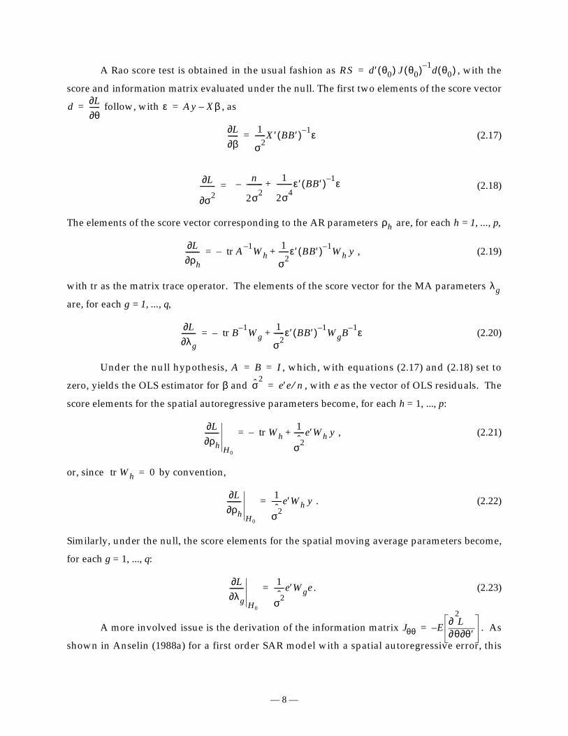
A Rao score test is obtained in the usual fashion as , with the
score and information matrix evaluated under the null. The first two elements of the score vector
follow, with , as
(2.17)
(2.18)
The elements of the score vector corresponding to the AR parameters are, for each h = 1, ..., p,
, (2.19)
with tr as the matrix trace operator. The elements of the score vector for the MA parameters
are, for each g = 1, ..., q,
(2.20)
Under the null hypothesis, , which, with equations (2.17) and (2.18) set to
zero, yields the OLS estimator for β and , with e as the vector of OLS residuals. The
score elements for the spatial autoregressive parameters become, for each h = 1, ..., p:
, (2.21)
or, since by convention,
. (2.22)
Similarly, under the null, the score elements for the spatial moving average parameters become,
for each g = 1, ..., q:
. (2.23)
A more involved issue is the derivation of the information matrix . As
shown in Anselin (1988a) for a first order SAR model with a spatial autoregressive error, this
RS d ′ θ0( ) J θ0( ) 1– d θ0( )=
d L∂θ∂
------= ε Ay Xβ–=
L∂β∂
------1
σ2------X ′ BB ′( ) 1– ε=
L∂
σ2∂---------
n
2σ2---------–
1
2σ4---------ε′ BB ′( ) 1– ε+=
ρh
L∂ρh∂
-------- tr A 1– Wh–1
σ2------ε′ BB′( ) 1– Wh y+=
λg
L∂λg∂
-------- tr B 1– Wg–1
σ2------ε′ BB ′( ) 1– WgB 1– ε+=
A B I= =
σ2
e ′ e n⁄=
L∂ρh∂
--------
H0
tr Wh–1
σ2ˆ------e ′Wh y+=
tr Wh 0=
L∂ρh∂
--------
H0
1
σ2ˆ------e ′Wh y=
L∂λg∂
--------
H0
1
σ2ˆ------e ′Wge=
Jθθ E θ θ′∂
2
∂∂ L
–=
— 9 —
information matrix is not block diagonal between the parameters of the model ( ) and those
of the error covariance ( ). This result also holds for the more general model considered
here. For ease of notation, consider the information matrix partitioned into four blocks: , for
the diagonal block of k +1 by k + 1 elements corresponding to β and ; for the diagonal
block of p + q by p + q elements corresponding to the parameters and ; and (and its
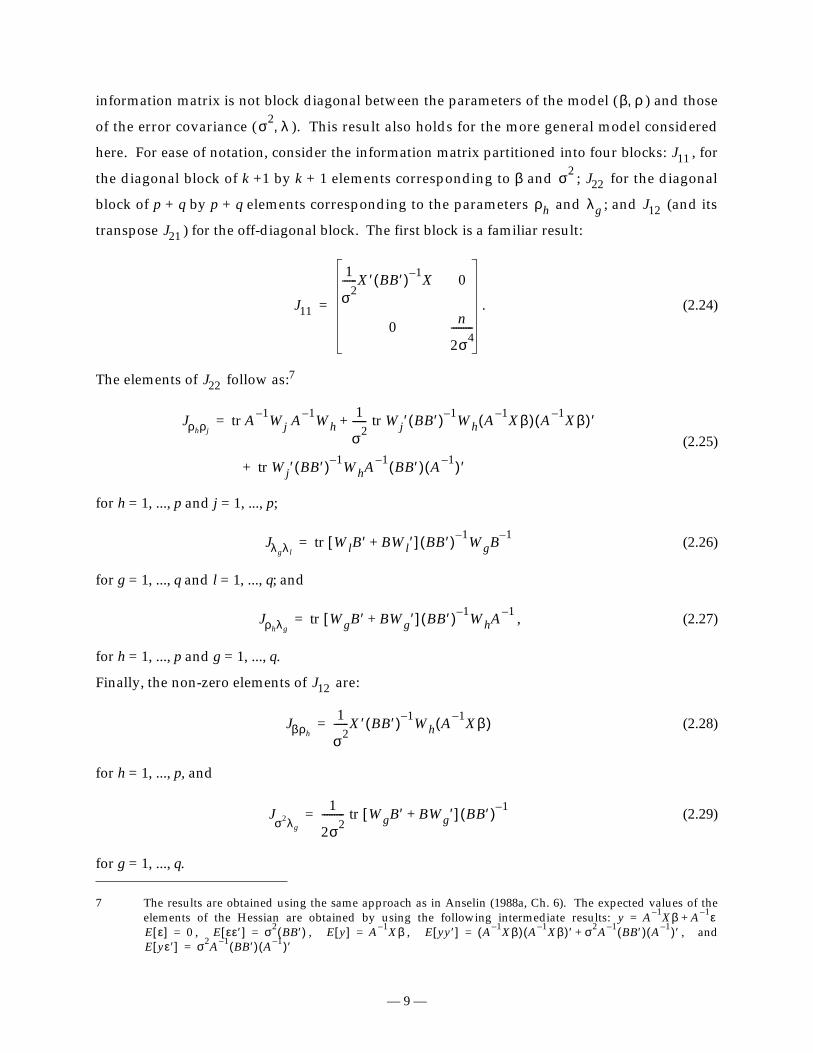
transpose ) for the off-diagonal block. The first block is a familiar result:
. (2.24)
The elements of follow as:7
(2.25)
for h = 1, ..., p and j = 1, ..., p;
(2.26)
for g = 1, ..., q and l = 1, ..., q; and
, (2.27)
for h = 1, ..., p and g = 1, ..., q.
Finally, the non-zero elements of are:
(2.28)
for h = 1, ..., p, and
(2.29)
for g = 1, ..., q.
7 The results are obtained using the same approach as in Anselin (1988a, Ch. 6). The expected values of theelements of the Hessian are obtained by using the following intermediate results:
, , , , and
β ρ,
σ2 λ,
J11
σ2 J22
ρh λg J12
J21
J11
1
σ2------X ′ BB ′( ) 1– X 0
0n
2σ4---------
=
J22
y A 1– Xβ A 1– ε+=E ε[ ] 0= E εε′[ ] σ 2 BB′( )= E y[ ] A 1– Xβ= E yy ′[ ] A 1– Xβ( ) A 1– Xβ( )′ σ2A 1– BB′( ) A 1–( )′+=E yε′[ ] σ 2A 1– BB ′( ) A 1–( )′=
Jρhρjtr A 1– Wj A 1– Wh
1
σ2------ tr Wj ′ BB ′( ) 1– Wh A 1– Xβ( ) A 1– Xβ( )′+=
tr Wj ′ BB ′( ) 1– WhA 1– BB′( ) A 1–( )′+
Jλgλ ltr WlB ′ BWl ′+[ ] BB ′( ) 1– WgB 1–
=
Jρhλgtr WgB ′ BWg ′+[ ] BB ′( ) 1– WhA 1–
=
J12
Jβρh
1
σ2------X ′ BB ′( ) 1– Wh A 1– Xβ( )=
Jσ2λg
1
2σ2--------- tr WgB ′ BWg ′+[ ] BB′( ) 1–
=
— 10 —
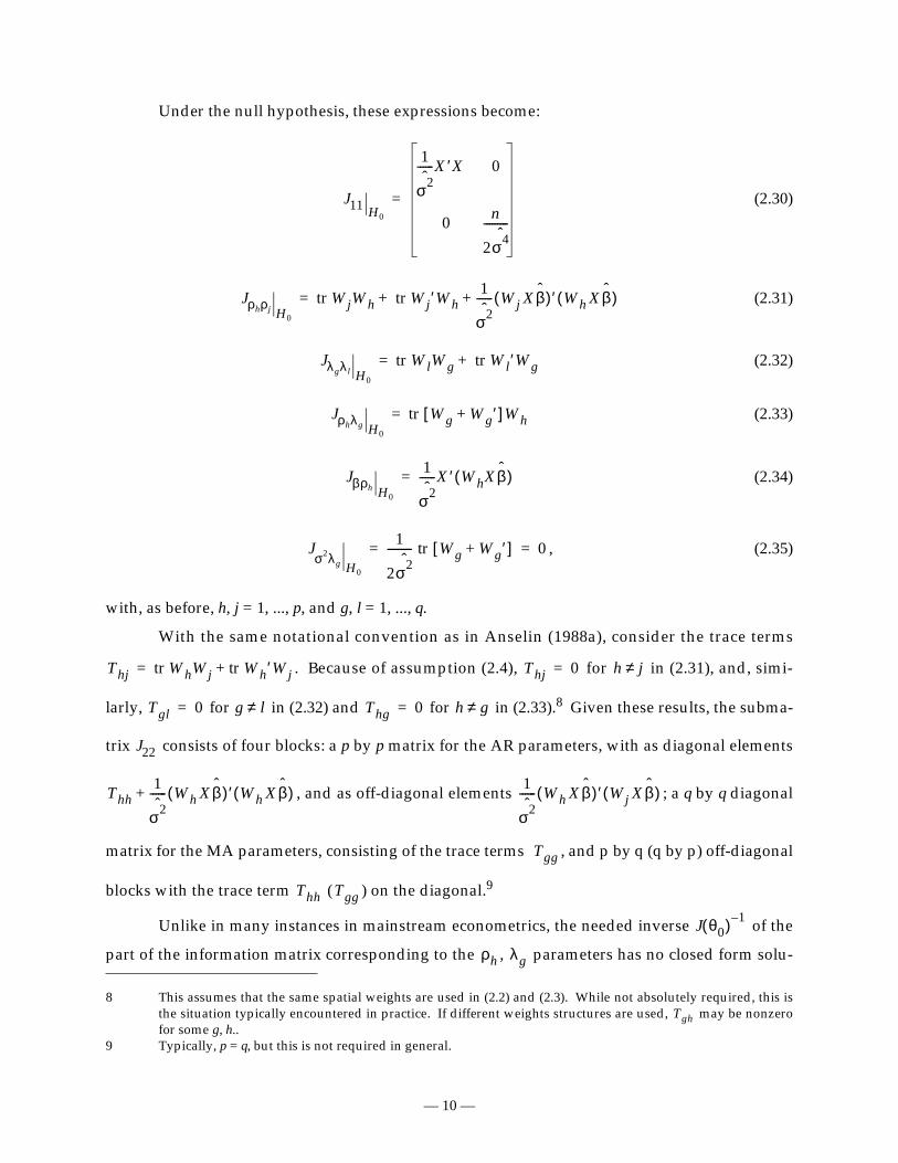
Under the null hypothesis, these expressions become:
(2.30)
(2.31)
(2.32)
(2.33)
(2.34)
, (2.35)
with, as before, h, j = 1, ..., p, and g, l = 1, ..., q.
With the same notational convention as in Anselin (1988a), consider the trace terms
. Because of assumption (2.4), for in (2.31), and, simi-
larly, for in (2.32) and for in (2.33).8 Given these results, the subma-
trix consists of four blocks: a p by p matrix for the AR parameters, with as diagonal elements
, and as off-diagonal elements ; a q by q diagonal
matrix for the MA parameters, consisting of the trace terms , and p by q (q by p) off-diagonal
blocks with the trace term ( ) on the diagonal.9
Unlike in many instances in mainstream econometrics, the needed inverse of the
part of the information matrix corresponding to the , parameters has no closed form solu-
8 This assumes that the same spatial weights are used in (2.2) and (2.3). While not absolutely required, this isthe situation typically encountered in practice. If different weights structures are used, may be nonzerofor some g, h..
9 Typically, p = q, but this is not required in general.
J11 H0
1
σ2ˆ------X ′X 0
0n
2σ4ˆ---------
=
Jρhρj H0
tr WjWh tr Wj ′Wh1
σ2ˆ------ Wj Xβˆ( )′ Wh Xβˆ( )+ +=
Jλgλ l H0
tr WlWg tr Wl ′Wg+=
Jρhλg H0
tr Wg Wg ′+[ ] Wh=
Jβρh H0
1
σ2ˆ------X ′ WhXβˆ( )=
Jσ2λg H0
1
2σ2ˆ--------- tr Wg Wg ′+[ ] 0= =
Thj tr WhWj tr Wh ′Wj+= Thj 0= h j≠
Tgl 0= g l≠ Thg 0= h g≠
Tgh
J22
Thh1
σ2ˆ------ Wh Xβˆ( )′ Wh Xβˆ( )+
1
σ2ˆ------ Wh Xβˆ( )′ Wj Xβˆ( )
Tgg
Thh Tgg
J θ0( ) 1–
ρh λg
— 11 —
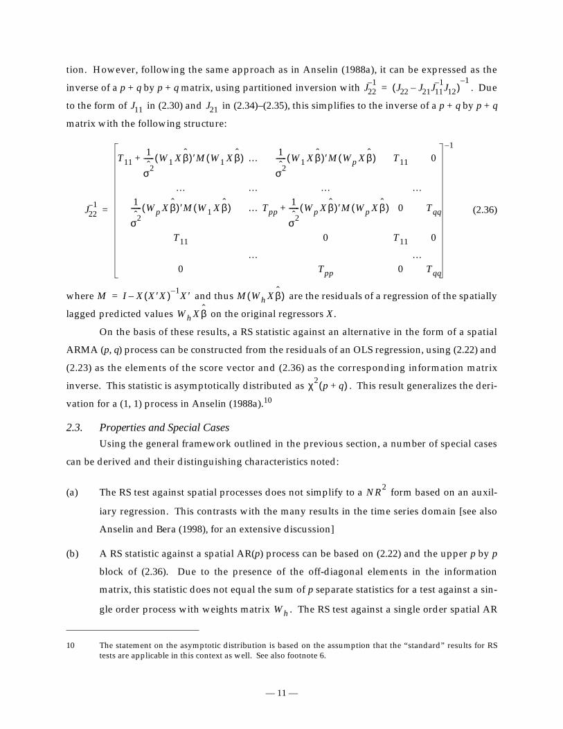
tion. However, following the same approach as in Anselin (1988a), it can be expressed as the
inverse of a p + q by p + q matrix, using partitioned inversion with . Due
to the form of in (2.30) and in (2.34)–(2.35), this simplifies to the inverse of a p + q by p + q
matrix with the following structure:
(2.36)
where and thus are the residuals of a regression of the spatially
lagged predicted values on the original regressors X.
On the basis of these results, a RS statistic against an alternative in the form of a spatial
ARMA (p, q) process can be constructed from the residuals of an OLS regression, using (2.22) and
(2.23) as the elements of the score vector and (2.36) as the corresponding information matrix
inverse. This statistic is asymptotically distributed as . This result generalizes the deri-
vation for a (1, 1) process in Anselin (1988a).10
2.3. Properties and Special Cases
Using the general framework outlined in the previous section, a number of special cases
can be derived and their distinguishing characteristics noted:
(a) The RS test against spatial processes does not simplify to a form based on an auxil-
iary regression. This contrasts with the many results in the time series domain [see also
Anselin and Bera (1998), for an extensive discussion]
(b) A RS statistic against a spatial AR(p) process can be based on (2.22) and the upper p by p
block of (2.36). Due to the presence of the off-diagonal elements in the information
matrix, this statistic does not equal the sum of p separate statistics for a test against a sin-
gle order process with weights matrix . The RS test against a single order spatial AR
10 The statement on the asymptotic distribution is based on the assumption that the “standard” results for RStests are applicable in this context as well. See also footnote 6.
J221– J22 J21J11
1– J12–( )1–
=
J11 J21
J221–
T111
σ2ˆ------ W1 Xβˆ( )′M W1 Xβˆ( )+ … 1
σ2ˆ------ W1 Xβˆ( )′M Wp Xβˆ( ) T11 0
… … … …1
σ2ˆ------ Wp Xβˆ( )′M W1 Xβˆ( ) … Tpp
1
σ2ˆ------ Wp Xβˆ( )′M Wp Xβˆ( )+ 0 Tqq
T11 0 T11 0
… …0 Tpp 0 Tqq
1–
=
M I X X ′X( ) 1– X ′–= M Wh Xβˆ( )
Wh Xβˆ
χ2 p q+( )
NR2
Wh
— 12 —
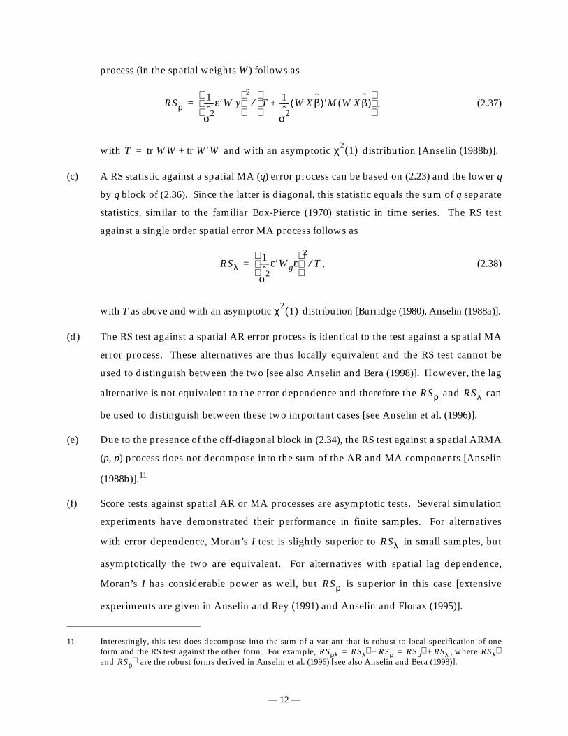
process (in the spatial weights W) follows as
, (2.37)
with and with an asymptotic distribution [Anselin (1988b)].
(c) A RS statistic against a spatial MA (q) error process can be based on (2.23) and the lower q
by q block of (2.36). Since the latter is diagonal, this statistic equals the sum of q separate
statistics, similar to the familiar Box-Pierce (1970) statistic in time series. The RS test
against a single order spatial error MA process follows as
, (2.38)
with T as above and with an asymptotic distribution [Burridge (1980), Anselin (1988a)].
(d) The RS test against a spatial AR error process is identical to the test against a spatial MA
error process. These alternatives are thus locally equivalent and the RS test cannot be
used to distinguish between the two [see also Anselin and Bera (1998)]. However, the lag
alternative is not equivalent to the error dependence and therefore the and can
be used to distinguish between these two important cases [see Anselin et al. (1996)].
(e) Due to the presence of the off-diagonal block in (2.34), the RS test against a spatial ARMA
(p, p) process does not decompose into the sum of the AR and MA components [Anselin
(1988b)].11
(f) Score tests against spatial AR or MA processes are asymptotic tests. Several simulation
experiments have demonstrated their performance in finite samples. For alternatives
with error dependence, Moran’s I test is slightly superior to in small samples, but
asymptotically the two are equivalent. For alternatives with spatial lag dependence,
Moran’s I has considerable power as well, but is superior in this case [extensive
experiments are given in Anselin and Rey (1991) and Anselin and Florax (1995)].
11 Interestingly, this test does decompose into the sum of a variant that is robust to local specification of oneform and the RS test against the other form. For example, , where and are the robust forms derived in Anselin et al. (1996) [see also Anselin and Bera (1998)].
RSρ1
σ2ˆ------ε′W y
2
T 1
σ2ˆ------ W Xβˆ( )′M W Xβˆ( )+
⁄=
T tr WW tr W′W+= χ21( )
RSλ1
σ2ˆ------ε′Wgε
2
T⁄=
χ21( )
RSρ RSλ
RSρλ RSλ∗ RSρ+ RSρ∗ RSλ+= = RSλ∗RSρ∗
RSλ
RSρ
— 13 —
3. A Rao Score Test against Spatial Error Components
3.1. General Principles
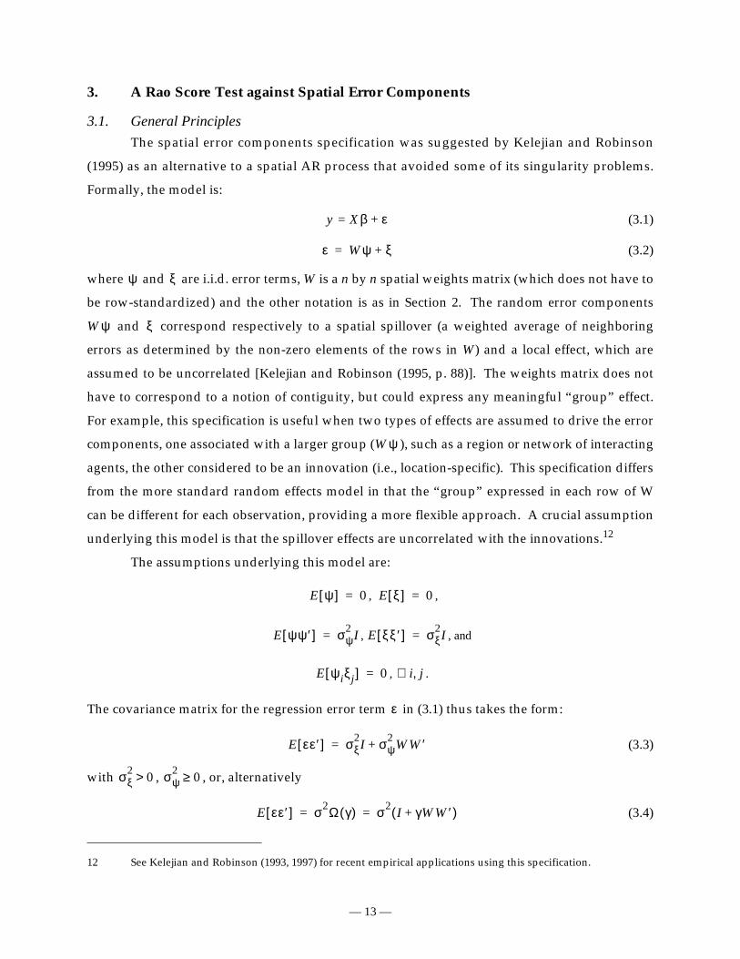
The spatial error components specification was suggested by Kelejian and Robinson
(1995) as an alternative to a spatial AR process that avoided some of its singularity problems.
Formally, the model is:
(3.1)
(3.2)
where and are i.i.d. error terms, W is a n by n spatial weights matrix (which does not have to
be row-standardized) and the other notation is as in Section 2. The random error components
W and correspond respectively to a spatial spillover (a weighted average of neighboring
errors as determined by the non-zero elements of the rows in W) and a local effect, which are
assumed to be uncorrelated [Kelejian and Robinson (1995, p. 88)]. The weights matrix does not
have to correspond to a notion of contiguity, but could express any meaningful “group” effect.
For example, this specification is useful when two types of effects are assumed to drive the error
components, one associated with a larger group (W ), such as a region or network of interacting
agents, the other considered to be an innovation (i.e., location-specific). This specification differs
from the more standard random effects model in that the “group” expressed in each row of W
can be different for each observation, providing a more flexible approach. A crucial assumption
underlying this model is that the spillover effects are uncorrelated with the innovations.12
The assumptions underlying this model are:
, ,
, , and
, .
The covariance matrix for the regression error term in (3.1) thus takes the form:
(3.3)
with , , or, alternatively
(3.4)
12 See Kelejian and Robinson (1993, 1997) for recent empirical applications using this specification.
y Xβ= ε+
ε Wψ ξ+=
ψ ξ
ψ ξ
ψ
E ψ[ ] 0= E ξ[ ] 0=
E ψψ′[ ] σ ψ2 I= E ξξ′[ ] σ ξ
2I=
E ψiξ j[ ] 0= i j,∀
ε
E εε′[ ] σ ξ2I σψ
2 WW′+=
σξ2
0> σψ2
0≥
E εε′[ ] σ 2Ω γ( ) σ2 I γWW ′+( )= =
— 14 —
where is the parameter vector, with and , the ratio of
the spatial spillover variance relative to the local variance.13 Since is symmetric and non-
negative definite and I is positive definite, the matrix is always positive definite. Kelejian and
Robinson derive an estimator for the model (3.1)–(3.3) based on the General Method of Moments
(GMM), in which a consistent estimator for the variance components is obtained from an auxil-
iary regression using OLS.14 A specification test for spatial autocorrelation is formulated as an
asymptotic significance test on the parameter in (3.3) [Kelejian and Robinson (1993, p. 304)].
Estimation of the parameters in this model can also be based on maximum likelihood,
with the additional assumption of normal distributions for and . The model is a special case
of a non-spherical error variance covariance matrix, but unlike the standard case [e.g., Magnus
(1978, pp. 283–284), Serfling (1980, pp. 143–149), Godfrey (1988, pp. 6–8)], special care must be
taken to establish sufficient conditions that impose distance decay and bounds on the heteroge-
neity.15
In the standard maximum likelihood context, one of the basic regularity conditions
requires that the true parameter values for are interior points of a finite dimensional, closed
and bounded parameter space . For a null hypothesis of the form in model (3.4), the
true parameter value is on the boundary of the parameter space and hence does not satisfy this
condition. As a consequence, and assuming that the same conditions are required in the spatial
model, hypothesis tests for based on a standard implementation of LR or W tests will not have
the expected asymptotic distribution under the null hypothesis. This same problem is
encountered in a number of econometric specifications involving error components and has
received considerable attention in the literature [classic references are Chernoff (1954), Moran
(1971) and Chant (1974); see also Godfrey (1988, pp. 92–98) and Bera et al. (1996) for recent
reviews]. A major result is that in contrast to the LR and W tests, the score test is unaffected by
this condition.
3.2. Score Test
The model with error covariance matrix (3.4) is a special case of a non-spherical error in a
linear regression. Its log-likelihood, score and information matrix can be derived in a straightfor-
ward manner using the general principles outlined in Magnus (1978) and Breusch (1980), among
13 Note the similarity between (3.3) and the error covariance for the model with a spatial MA error process,(2.10), for which . Both specifications result in a small number ofnonzero elements in the covariance matrix (corresponding to the first and/or second order neighbors).
14 No non-negativity constraint is imposed in this auxiliary regression.15 See also the discussion in footnote 6. Note that Kelejian and Robinson (1993) establish consistency of the
GMM estimator for explicitly without resorting to normality.
θ σ2 γ,[ ]′= σ2 σξ2
0>= γ σψ2 σξ
2⁄ 0≥=
WW ′
E εε′[ ] σ 2 I λ W W′+( ) λ2WW′+ +[ ]=
Ω
σψ2
ψ ξ
β
θ
Θ H0: γ 0=
γ
χ21( )
— 15 —
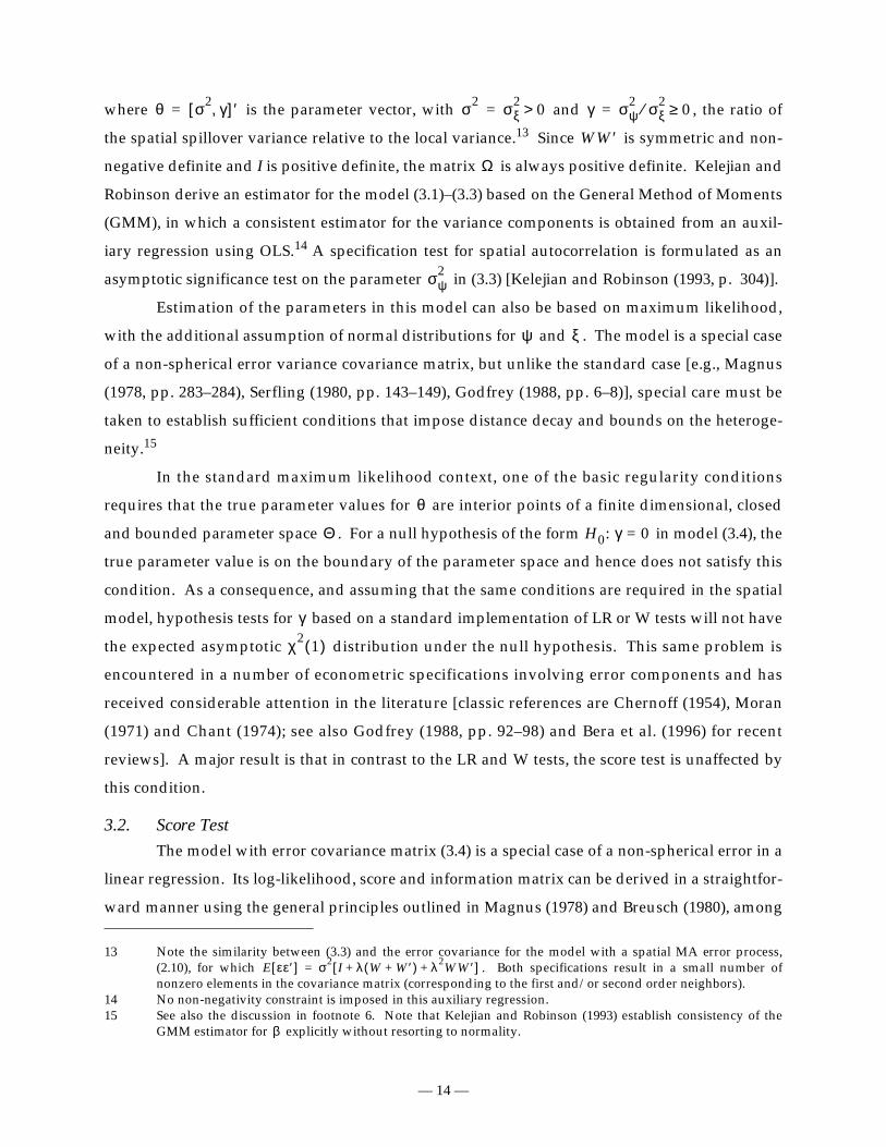
others. In contrast to the spatial ARMA model considered in the previous section, for this case
the information matrix is block diagonal between the elements corresponding to and those for
the error parameter vector . Therefore, to obtain the information matrix for the RS
statistic, only the submatrix corresponding to needs to be considered. The following expres-
sions follow for the log-likelihood , the score vector and the relevant part of the infor-
mation matrix, , using , and tr as the matrix trace operator,
(3.5)
(3.6)
and
(3.7)
A Rao score test for the null hypothesis against the alternative is
obtained as , with the score and information matrix evaluated under
the null, or, with , where I is a n by n identity matrix. The corresponding expressions
are:
(3.8)
(3.9)
β
θ σ2 γ,[ ]′=
θ
L d L∂θ∂
------=
Jθθ E θ θ′∂
2
∂∂ L
–= ε y Xβ–=
L n2--- 2π( )ln–
n2--- σ2( )ln–
12--- Ωln–
1
2σ2---------ε′Ω 1– ε–=
d
n
2σ2---------–
1
2σ4---------ε′Ω 1– ε+
12---tr Ω 1– WW ′–
1
2σ2---------ε′Ω 1– WW ′Ω 1– ε+
=
Jθθ
n
2σ4---------
1
2σ2---------tr Ω 1– WW ′
1
2σ2---------tr Ω 1– WW ′ 1
2---tr Ω 1– WW ′Ω 1– WW ′
=
H0: γ 0= H1: γ 0>
RSγ d ′ θ0( )J θ0( ) 1– d θ0( )=
Ω 1– I=
d θ0( ) 12---tr WW ′–
1
2σ2
---------e ′WW ′ e+=
J θ0( )
n
2σ4
---------1
2σ2
---------tr WW ′
1
2σ2
---------tr WW′ 12---tr WW′WW ′
=
— 16 —
where e is a vector of OLS residuals and . To simplify notation, set and
. Using partitioned inversion, the inverse of the 2, 2 element of (3.5) then fol-
lows as:
(3.10)
Combining all terms, the test statistic is obtained as
.16 (3.11)
As in the cases considered in Section 2, this test requires only the results from OLS estimation,
and, under , .17 In practice, the test can also be implemented by comparing the
positive square root of , or to the one-sided significance levels of a standard nor-
mal variate.
3.3. Small Sample Performance
While an extensive investigation is beyond the scope of the current paper, some limited
insight into the performance of the test is obtained from a small set of Monte Carlo simulation
experiments.18 The data are generated over a regular square lattice, using a standard normal dis-
tribution for the error term ε and a fixed n by 2 matrix X, with the first column consisting of ones
and the second column generated as a uniformly distributed random variate between 0 and 10.19
Under the alternative hypothesis, the proper covariance structure is generated for the error term
by applying a Choleski decomposition to the matrix using a first order rook con-
tiguity for W and . Five sample sizes are
considered, n = 25 (5 x 5), 49 (7 x 7), 81 (9 x 9), 121 (11 x 11) and 400 (20 x 20).
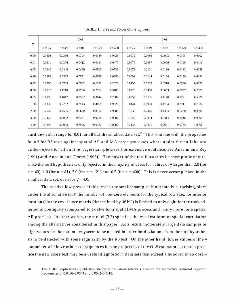
The results are reported in Table 1, with the empirical Type I errors based on the one-
sided test. All results are for 10,000 replications, using nominal significance levels of 0.05 and
0.01. The size of the test is acceptable (given in the first row of the table), yielding a slight under-
rejection relative to the nominal level for 0.05, but rejection levels remain within the two stan-
16 An interesting interpretation of this statistics, suggested by Anil Bera, is to consider it as a moment test,
where the interest focuses on the moment condition . Under the null hypothesis, with
, this condition is statisfied.17 Again, this assumes that the standard asymptotic results for RS tests are applicable. See also footnote 6.18 A more comprehensive analysis and comparison to other tests is treated in Anselin and Moreno (2000).19 Under the null hypothesis, this yields an average of around 0.94 for the OLS regressions.
σ2
e ′ e n⁄= tr WW′ T1=
tr WW ′WW ′ T2=
J γγ θ0( ) 2 T2
T1( )2
n-------------–
1–
=
RSγe ′WW′ e
σ2
-------------------- T1–2
2 T2
T1( )2
n-------------–
⁄=
E ε′Wεε′ε
------------- T1=
E ε′ε[ ] σ 2I=
H0 RSγD
χ21( )→
RSγ zγ RSγ=
R2
Ω I γWW ′+=
γ 0.00 0.01 0.05 0.10 0.25 0.50 0.75 1.0 2.0 3.0 4.0, , , , , , , , , ,=
zγ
— 17 —
dard deviation range for 0.01 for all but the smallest data set.20 This is in line with the properties
found for RS tests against spatial AR and MA error processes where under the null the test
under-rejects for all but the largest sample sizes [for extensive evidence, see Anselin and Rey
(1991) and Anselin and Florax (1995)]. The power of the test illustrates its asymptotic nature,
since the null hypothesis is only rejected in the majority of cases for values of γ larger than 2.0 (for
n = 49), 1.0 (for n = 81), 2.0 (for n = 121) and 0.5 (for n = 400). This is never accomplished in the
smallest data set, even for γ = 4.0.
The relative low power of this test in the smaller samples is not totally surprising, since
under the alternative (3.4) the number of non-zero elements for the typical row (i.e., for interior
locations) in the covariance matrix (determined by ) is limited to only eight for the rook cri-
terion of contiguity (compared to twelve for a spatial MA process and many more for a spatial
AR process). In other words, the model (3.3) specifies the weakest form of spatial correlation
among the alternatives considered in this paper. As a result, moderately large data samples or
high values for the parameter γ seem to be needed in order for deviations from the null hypothe-
sis to be detected with some regularity by the RS test. On the other hand, lower values of the γ
parameter will have minor consequences for the properties of the OLS estimator, so that in prac-
tice the new score test may be a useful diagnostic in data sets that exceed a hundred or so obser-
TABLE 1: Size and Power of the Test
0.05 0.01
n = 25 n = 49 n = 81 n = 121 n = 400 n = 25 n = 49 n = 81 n = 121 n = 400
0.00 0.0303 0.0356 0.0394 0.0389 0.0433 0.0072 0.0086 0.0093 0.0105 0.0102
0.01 0.0311 0.0376 0.0412 0.0414 0.0477 0.0074 0.0087 0.0099 0.0110 0.0118
0.05 0.0349 0.0440 0.0469 0.0505 0.0739 0.0076 0.0101 0.0130 0.0122 0.0185
0.10 0.0393 0.0523 0.0551 0.0670 0.0982 0.0098 0.0144 0.0166 0.0189 0.0280
0.25 0.0500 0.0769 0.0992 0.1190 0.2372 0.0135 0.0203 0.0310 0.0386 0.0892
0.50 0.0813 0.1218 0.1760 0.2282 0.5188 0.0220 0.0400 0.0653 0.0937 0.2820
0.75 0.1096 0.1817 0.2557 0.3644 0.7587 0.0352 0.0715 0.1120 0.1771 0.5321
1.00 0.1339 0.2292 0.3543 0.4869 0.9026 0.0444 0.0959 0.1764 0.2711 0.7532
2.00 0.2529 0.4535 0.6620 0.8107 0.9985 0.1036 0.2465 0.4364 0.6220 0.9911
3.00 0.3425 0.6052 0.8241 0.9288 1.0000 0.1625 0.3914 0.6414 0.8216 0.9999
4.00 0.4190 0.7043 0.8996 0.9737 1.0000 0.2135 0.4891 0.7631 0.9135 1.0000
20 The 10,000 replications yield two standard deviation intervals around the respective nominal rejectionfrequencies of 0.0466–0.0544 and 0.0082–0.0118.
zγ
γ
WW ′
— 18 —
vations. However, before endorsing this test statistic without reservations, a number of issues
need to be further investigated, such as the extent to which its properties are maintained when
the error term is non-normal, and the comparison of its power to that of alternatives such as LR
and W tests that take into account the censored nature of the distribution of the estimators, as
well as procedures based on GMM estimation.
4. A Rao Score Test against Direct Representation of Spatial Covariance
4.1. General Principles
Under the direct representation form of spatial autocorrelation, the elements of the error
covariance matrix are specified as an inverse function of distance. Formally,
, (4.1)
where and are regression disturbance terms, is the error variance, is the distance
separating observations (locations) i and j, and f is a distance decay function such that
and , with as a p by 1 vector of parameters on an open subset of . This
form is closely related to the variogram model used in geostatistics, although with stricter
assumptions regarding stationarity and isotropy.21 Using (4.1) for individual elements, the full
error covariance matrix follows as
(4.2)
where, because of the scaling factor , the matrix must be a positive definite spatial
correlation matrix, with and , .22
Estimation of regression models that incorporate an error covariance of this form has
been explored in the statistical literature by Mardia and Marshall (1984), Warnes and Ripley
(1987), Mardia and Watkins (1989), and Mardia (1990), among others. In spatial econometrics,
models of this type have been used primarily in the analysis of urban housing markets, e.g., in
Dubin (1988, 1992) and Olmo (1995). While this specification has a certain intuition, in the sense
21 The specification of spatial covariance functions is not arbitrary, and a number of conditions must be satisfiedin order for the model to be “valid” [details are given in Cressie (1993, pp. 61–63, 67–68 and 84–86)]. For astationary process, the covariance function must be positive definite and it is required that as ,which is ensured by the conditions spelled out here. Furthermore, most models only consider positive spatialautocorrelation in this context. An exception is the so-called wave variogram, which allows both positive andnegative correlation due to the periodicity of the process. This model has not seen application outside thephysical sciences and is not considered here.
22 is ensured by selecting a functional form for f such that for . Also, in contrast towhat holds for the spatial process models discussed in Section 2, the error terms are not heteroskedastic inthis specification, unless this heteroskedasticity is introduced explicitly. In order to focus the discussion onthe aspects of spatial autocorrelation, this is excluded here.
Cov εiεj[ ] σ 2f dij ϕ,( )=
εi εj σ2 dijf∂d∂
------- 0<
f dij ϕ,( ) 1≤ ϕ Φ∈ Φ Rp
f 0→ dij ∞→
E εε′[ ] σ 2Ω dij ϕ,( )=
σ2 Ω dij ϕ,( )
ωii 1= ωij 1≤ i j,∀
ωi i 1= f dij ϕ,( ) 1= dij 0=εi
— 19 —
that it incorporates an explicit notion of spatial clustering as a function of the distance separating
two observations (i.e., positive spatial correlation), it is also fraught with a number of estimation
and identification problems. Mardia and Marshall (1984, pp. 138–139) spell out the assumptions
under which maximum likelihood yields a consistent and asymptotically normal estimator. For
the purposes of the discussion here, it suffices to note that the error covariance matrix should be
twice differentiable and continuous in the parameters . In addition, the elements of the covari-
ance matrix, and their first and second partial derivatives should be absolutely summable.23 The
importance of these conditions is that they impose constraints on the parameter space as well
as on the type of distance decay functions f.
Several specifications suggested in the literature do not meet these estimability and iden-
tifiability conditions. For example, as illustrated in Mardia (1990, p. 212), the popular geostatisti-
cal spherical model with range parameter is not twice differentiable. In spatial econometrics,
Dubin (1988, 1992) proposed the use of a negative exponential correlogram. In her specification,
the error covariance matrix is of the form [Dubin (1988, p. 467)]:
(4.3)
with
, (4.4)
where is the distance between observations i and j, and is a parameter. In Dubin (1992, eq.
2)24 a slight variant is introduced that contains an additional parameter , such that
. (4.5)
Clearly, in (4.3) and in (4.5) are not separately identifiable. Dubin (1992, p. 445) suggests
the use of LR to test for spatial autocorrelation, either as a test on the significance of the parame-
ter in (4.4) [Dubin (1988, p. 473] or on the joint significance of and in (4.5) [Dubin (1992,
p. 445]. However, upon closer examination, it turns out that this approach is problematic. Apart
from the identification problem in (4.5), a null hypothesis of the form : does not corre-
spond to an interior point of the parameter space and hence does not satisfy the regularity condi-
tions for ML, similar to the situation encountered in Section 3. At first sight, this could be fixed
by means of a straightforward reparametrization to , but under the null of
23 These conditions are similar in spirit to the conditions formulated in Magnus (1978) and Mandy and Martins-Filho (1994) for general non-spherical error models. However, in the spatial case, the standard regularlityconditions do not apply directly and further conditions are needed as well (see also footnote 6).
24 The specification (4.5) was originally suggested in Dubin (1988, fn. 8) but not implemented in that paper.
ϕ
Φ
E εε′[ ] σ 2K=
Kij exp dij– b2⁄( )=
dij b2
b1
Kij b1 exp dij– b2⁄( )=
σ2 b1
b2 b1 b2
H0 b2 0=
Kij exp b3dij
–( )=
— 20 —
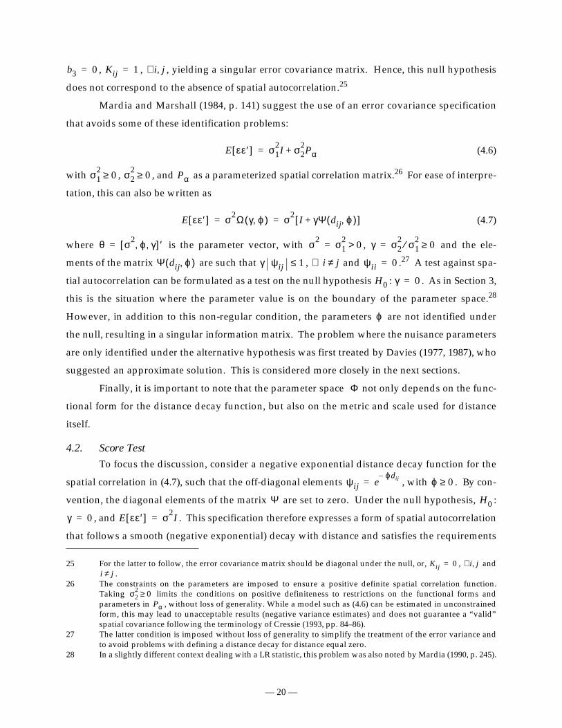
, , , yielding a singular error covariance matrix. Hence, this null hypothesis
does not correspond to the absence of spatial autocorrelation.25
Mardia and Marshall (1984, p. 141) suggest the use of an error covariance specification
that avoids some of these identification problems:
(4.6)
with , , and as a parameterized spatial correlation matrix.26 For ease of interpre-
tation, this can also be written as
(4.7)
where is the parameter vector, with , and the ele-
ments of the matrix are such that , and .27 A test against spa-
tial autocorrelation can be formulated as a test on the null hypothesis : . As in Section 3,
this is the situation where the parameter value is on the boundary of the parameter space.28
However, in addition to this non-regular condition, the parameters are not identified under
the null, resulting in a singular information matrix. The problem where the nuisance parameters
are only identified under the alternative hypothesis was first treated by Davies (1977, 1987), who
suggested an approximate solution. This is considered more closely in the next sections.
Finally, it is important to note that the parameter space not only depends on the func-
tional form for the distance decay function, but also on the metric and scale used for distance
itself.
4.2. Score Test
To focus the discussion, consider a negative exponential distance decay function for the
spatial correlation in (4.7), such that the off-diagonal elements , with . By con-
vention, the diagonal elements of the matrix are set to zero. Under the null hypothesis, :
, and . This specification therefore expresses a form of spatial autocorrelation
that follows a smooth (negative exponential) decay with distance and satisfies the requirements
25 For the latter to follow, the error covariance matrix should be diagonal under the null, or, , and.
26 The constraints on the parameters are imposed to ensure a positive definite spatial correlation function.Taking limits the conditions on positive definiteness to restrictions on the functional forms andparameters in , without loss of generality. While a model such as (4.6) can be estimated in unconstrainedform, this may lead to unacceptable results (negative variance estimates) and does not guarantee a “valid”spatial covariance following the terminology of Cressie (1993, pp. 84–86).
27 The latter condition is imposed without loss of generality to simplify the treatment of the error variance andto avoid problems with defining a distance decay for distance equal zero.
28 In a slightly different context dealing with a LR statistic, this problem was also noted by Mardia (1990, p. 245).
b3 0= Kij 1= i j,∀
Kij 0= i j,∀i j≠
E εε′[ ] σ 12I σ2
2Pα+=
σ12
0≥ σ22
0≥ Pα
σ22
0≥Pα
E εε′[ ] σ 2Ω γ ϕ,( ) σ2 I γΨ dij ϕ,( )+[ ]= =
θ σ2 ϕ γ, ,[ ]′= σ2 σ12
0>= γ σ22 σ1
2⁄ 0≥=
Ψ dij ϕ,( ) γ ψij 1≤ i j≠∀ ψ ii 0=
H0 γ 0=
ϕ
Φ
ψij eϕdij–
= ϕ 0≥
Ψ H0
γ 0= E εε′[ ] σ 2I=
— 21 —
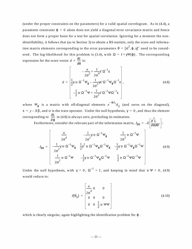
(under the proper constraints on the parameters) for a valid spatial correlogram. As in (4.4), a
parameter constraint alone does not yield a diagonal error covariance matrix and hence
does not form a proper basis for a test for spatial correlation. Ignoring for a moment the non-
identifiability, it follows that (as in Section 3) to obtain a RS statistic, only the score and informa-
tion matrix elements corresponding to the error parameters need to be consid-
ered. The log-likelihood for this problem is (3.4), with . The corresponding
expression for the score vector is:
, (4.8)
where is a matrix with off-diagonal elements (and zeros on the diagonal),
, and tr is the trace operator. Under the null hypothesis, , and thus the element
corresponding to in (4.8) is always zero, precluding its estimation.
Furthermore, consider the relevant part of the information matrix, :
(4.9)
Under the null hypothesis, with , , and keeping in mind that , (4.9)
would reduce to:
(4.10)
which is clearly singular, again highlighting the identification problem for .
ϕ 0=
θ σ2 ϕ γ, ,[ ]′=
Ω I γΨ ϕ( )+=
d L∂θ∂
------=
d
n
2σ2---------–
1
2σ4---------ε′Ω 1– ε+
12---γ tr Ω 1– Ψϕ
1
2σ2---------γε′Ω 1– ΨϕΩ 1– ε–
12---– tr Ω 1– Ψ 1
2σ2---------ε′Ω 1– ΨΩ 1– ε+
=
Ψϕ eϕdij–
dij
ε y Xβ–= γ 0=L∂ϕ∂
-------
Jθθ E θ θ′∂
2
∂∂ L
–=
Jθθ
n
2σ4--------- 1
2σ2---------– γ tr Ω 1– Ψϕ
1
2σ2--------- tr Ω 1– Ψ
1
2σ2---------– γ tr Ω 1– Ψϕ
12---γ2
tr Ω 1– ΨϕΩ 1– Ψϕ12---– γ tr Ω 1– ΨϕΩ 1– Ψ
1
2σ2--------- tr Ω 1– Ψ 1
2---– γ tr Ω 1– ΨϕΩ 1– Ψ 1
2--- tr Ω 1– ΨΩ 1– Ψ
=
γ 0= Ω 1– I= tr Ψ 0=
J θ0( )
n
2σ4--------- 0 0
0 0 0
0 012--- tr ΨΨ
=
ϕ
— 22 —
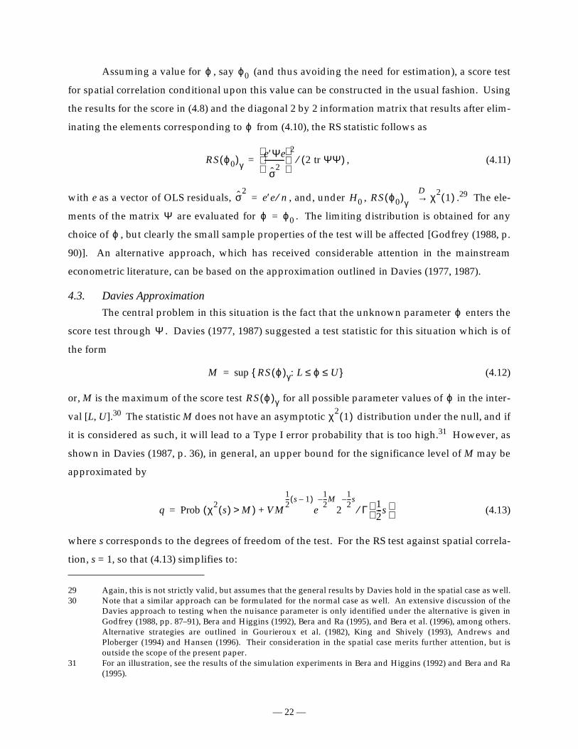
Assuming a value for , say (and thus avoiding the need for estimation), a score test
for spatial correlation conditional upon this value can be constructed in the usual fashion. Using
the results for the score in (4.8) and the diagonal 2 by 2 information matrix that results after elim-
inating the elements corresponding to from (4.10), the RS statistic follows as
, (4.11)
with e as a vector of OLS residuals, , and, under , .29 The ele-
ments of the matrix are evaluated for . The limiting distribution is obtained for any
choice of , but clearly the small sample properties of the test will be affected [Godfrey (1988, p.
90)]. An alternative approach, which has received considerable attention in the mainstream
econometric literature, can be based on the approximation outlined in Davies (1977, 1987).
4.3. Davies Approximation
The central problem in this situation is the fact that the unknown parameter enters the
score test through . Davies (1977, 1987) suggested a test statistic for this situation which is of
the form
(4.12)
or, M is the maximum of the score test for all possible parameter values of in the inter-
val [L, U].30 The statistic M does not have an asymptotic distribution under the null, and if
it is considered as such, it will lead to a Type I error probability that is too high.31 However, as
shown in Davies (1987, p. 36), in general, an upper bound for the significance level of M may be
approximated by
(4.13)
where s corresponds to the degrees of freedom of the test. For the RS test against spatial correla-
tion, s = 1, so that (4.13) simplifies to:
29 Again, this is not strictly valid, but assumes that the general results by Davies hold in the spatial case as well.30 Note that a similar approach can be formulated for the normal case as well. An extensive discussion of the
Davies approach to testing when the nuisance parameter is only identified under the alternative is given inGodfrey (1988, pp. 87–91), Bera and Higgins (1992), Bera and Ra (1995), and Bera et al. (1996), among others.Alternative strategies are outlined in Gourieroux et al. (1982), King and Shively (1993), Andrews andPloberger (1994) and Hansen (1996). Their consideration in the spatial case merits further attention, but isoutside the scope of the present paper.
31 For an illustration, see the results of the simulation experiments in Bera and Higgins (1992) and Bera and Ra(1995).
ϕ ϕ0
ϕ
RS ϕ0( )γe ′Ψe
σ2
----------- 2
2 tr ΨΨ( )⁄=
σ2
e ′ e n⁄= H0 RS ϕ0( )γD
χ21( )→
Ψ ϕ ϕ0=
ϕ
ϕ
Ψ
M sup RS ϕ( )γ: L ϕ U≤ ≤ =
RS ϕ( )γ ϕ
χ21( )
q Prob χ2 s( ) M>( ) VM
12--- s 1–( )
e
12---M–
2
12---s–
Γ 12---s
⁄+=
— 23 —
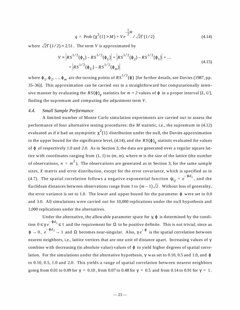
(4.14)
where . The term V is approximated by
(4.15)
where are the turning points of [for further details, see Davies (1987, pp.
35–36)]. This approximation can be carried out in a straightforward but computationally inten-
sive manner by evaluating the statistics for m + 2 values of in a proper interval [L, U],
finding the supremum and computing the adjustment term V.
4.4. Small Sample Performance
A limited number of Monte Carlo simulation experiments are carried out to assess the
performance of four alternative testing procedures: the M statistic, i.e., the supremum in (4.12)
evaluated as if it had an asymptotic distribution under the null, the Davies approximation
to the upper bound for the significance level, (4.14), and the statistic evaluated for values
of of respectively 1.0 and 2.0. As in Section 3, the data are generated over a regular square lat-
tice with coordinates ranging from (1, 1) to (m, m), where m is the size of the lattice (the number
of observations, ). The observations are generated as in Section 3, for the same sample
sizes, X matrix and error distribution, except for the error covariance, which is specified as in
(4.7). The spatial correlation follows a negative exponential function , and the
Euclidean distances between observations range from 1 to . Without loss of generality,
the error variance is set to 1.0. The lower and upper bound for the parameter were set to 0.0
and 3.0. All simulations were carried out for 10,000 replications under the null hypothesis and
1,000 replications under the alternatives.
Under the alternative, the allowable parameter space for is determined by the condi-
tion and the requirement for to be positive definite. This is not trivial, since as
, and becomes near-singular. Also, is the spatial correlation between
nearest neighbors, i.e., lattice vertices that are one unit of distance apart. Increasing values of
combine with decreasing (in absolute value) values of to yield higher degrees of spatial corre-
lation. For the simulations under the alternative hypothesis, was set to 0.10, 0.5 and 1.0, and
to 0.10, 0.5, 1.0 and 2.0. This yields a range of spatial correlation between nearest neighbors
going from 0.01 to 0.09 for , from 0.07 to 0.48 for and from 0.14 to 0.91 for .
q Prob χ21( ) M>( ) Ve
12---M–
2Γ 1 2⁄( )⁄+=
2Γ 1 2⁄( ) 2.51≈
V RS1 2⁄ ϕ1( ) RS1 2⁄ ϕL( )– RS1 2⁄ ϕ2( ) RS1 2⁄ ϕ1( )– …+ +≈
RS1 2⁄ ϕU( ) RS1 2⁄ ϕm( )–+
ϕ1 ϕ2 … ϕm, , , RS1 2⁄ ϕ( )
RS ϕ( )γ ϕ
χ21( )
RS ϕ( )γ
ϕ
n m2=
ψij eϕdij–
=
m 1–( ) 2
ϕ
γ ϕ,
0 γ eϕdij–
1≤≤ Ω
ϕ 0→ eϕdij–
1→ Ω γ e ϕ–
γ
ϕ
γ ϕ
γ 0.10= γ 0.5= γ 1=
— 24 —
The power of the statistics can thus be evaluated in function of an intuitive and quantifiable
notion of first order spatial autocorrelation.
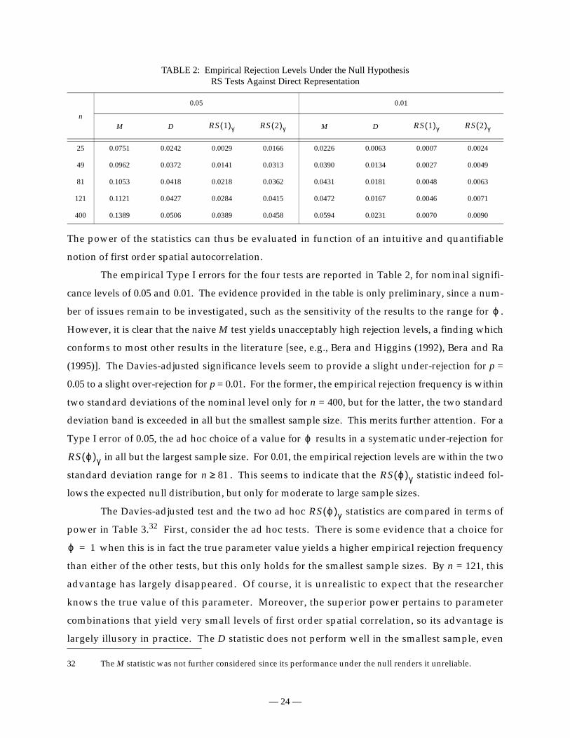
The empirical Type I errors for the four tests are reported in Table 2, for nominal signifi-
cance levels of 0.05 and 0.01. The evidence provided in the table is only preliminary, since a num-
ber of issues remain to be investigated, such as the sensitivity of the results to the range for .
However, it is clear that the naive M test yields unacceptably high rejection levels, a finding which
conforms to most other results in the literature [see, e.g., Bera and Higgins (1992), Bera and Ra
(1995)]. The Davies-adjusted significance levels seem to provide a slight under-rejection for p =
0.05 to a slight over-rejection for p = 0.01. For the former, the empirical rejection frequency is within
two standard deviations of the nominal level only for n = 400, but for the latter, the two standard
deviation band is exceeded in all but the smallest sample size. This merits further attention. For a
Type I error of 0.05, the ad hoc choice of a value for results in a systematic under-rejection for
in all but the largest sample size. For 0.01, the empirical rejection levels are within the two
standard deviation range for . This seems to indicate that the statistic indeed fol-
lows the expected null distribution, but only for moderate to large sample sizes.
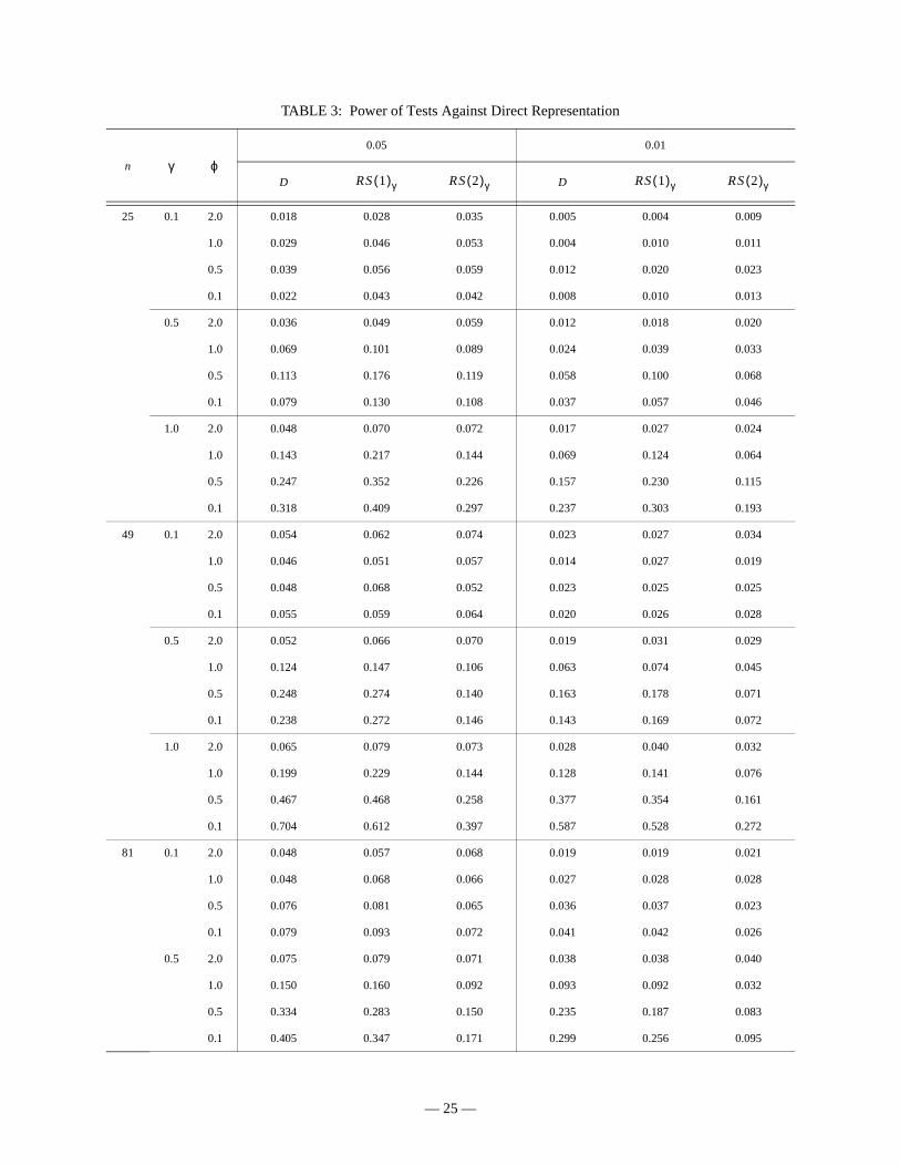
The Davies-adjusted test and the two ad hoc statistics are compared in terms of
power in Table 3.32 First, consider the ad hoc tests. There is some evidence that a choice for
when this is in fact the true parameter value yields a higher empirical rejection frequency
than either of the other tests, but this only holds for the smallest sample sizes. By n = 121, this
advantage has largely disappeared. Of course, it is unrealistic to expect that the researcher
knows the true value of this parameter. Moreover, the superior power pertains to parameter
combinations that yield very small levels of first order spatial correlation, so its advantage is
largely illusory in practice. The D statistic does not perform well in the smallest sample, even
TABLE 2: Empirical Rejection Levels Under the Null HypothesisRS Tests Against Direct Representation
n
0.05 0.01
M D M D
25 0.0751 0.0242 0.0029 0.0166 0.0226 0.0063 0.0007 0.0024
49 0.0962 0.0372 0.0141 0.0313 0.0390 0.0134 0.0027 0.0049
81 0.1053 0.0418 0.0218 0.0362 0.0431 0.0181 0.0048 0.0063
121 0.1121 0.0427 0.0284 0.0415 0.0472 0.0167 0.0046 0.0071
400 0.1389 0.0506 0.0389 0.0458 0.0594 0.0231 0.0070 0.0090
32 The M statistic was not further considered since its performance under the null renders it unreliable.
RS 1( )γ RS 2( )γ RS 1( )γ RS 2( )γ
ϕ
ϕ
RS ϕ( )γ
n 81≥ RS ϕ( )γ
RS ϕ( )γ
ϕ 1=
— 25 —
TABLE 3: Power of Tests Against Direct Representation
n
0.05 0.01
D D
25 0.1 2.0 0.018 0.028 0.035 0.005 0.004 0.009
1.0 0.029 0.046 0.053 0.004 0.010 0.011
0.5 0.039 0.056 0.059 0.012 0.020 0.023
0.1 0.022 0.043 0.042 0.008 0.010 0.013
0.5 2.0 0.036 0.049 0.059 0.012 0.018 0.020
1.0 0.069 0.101 0.089 0.024 0.039 0.033
0.5 0.113 0.176 0.119 0.058 0.100 0.068
0.1 0.079 0.130 0.108 0.037 0.057 0.046
1.0 2.0 0.048 0.070 0.072 0.017 0.027 0.024
1.0 0.143 0.217 0.144 0.069 0.124 0.064
0.5 0.247 0.352 0.226 0.157 0.230 0.115
0.1 0.318 0.409 0.297 0.237 0.303 0.193
49 0.1 2.0 0.054 0.062 0.074 0.023 0.027 0.034
1.0 0.046 0.051 0.057 0.014 0.027 0.019
0.5 0.048 0.068 0.052 0.023 0.025 0.025
0.1 0.055 0.059 0.064 0.020 0.026 0.028
0.5 2.0 0.052 0.066 0.070 0.019 0.031 0.029
1.0 0.124 0.147 0.106 0.063 0.074 0.045
0.5 0.248 0.274 0.140 0.163 0.178 0.071
0.1 0.238 0.272 0.146 0.143 0.169 0.072
1.0 2.0 0.065 0.079 0.073 0.028 0.040 0.032
1.0 0.199 0.229 0.144 0.128 0.141 0.076
0.5 0.467 0.468 0.258 0.377 0.354 0.161
0.1 0.704 0.612 0.397 0.587 0.528 0.272
81 0.1 2.0 0.048 0.057 0.068 0.019 0.019 0.021
1.0 0.048 0.068 0.066 0.027 0.028 0.028
0.5 0.076 0.081 0.065 0.036 0.037 0.023
0.1 0.079 0.093 0.072 0.041 0.042 0.026
0.5 2.0 0.075 0.079 0.071 0.038 0.038 0.040
1.0 0.150 0.160 0.092 0.093 0.092 0.032
0.5 0.334 0.283 0.150 0.235 0.187 0.083
0.1 0.405 0.347 0.171 0.299 0.256 0.095
γ ϕRS 1( )γ RS 2( )γ RS 1( )γ RS 2( )γ
— 26 —
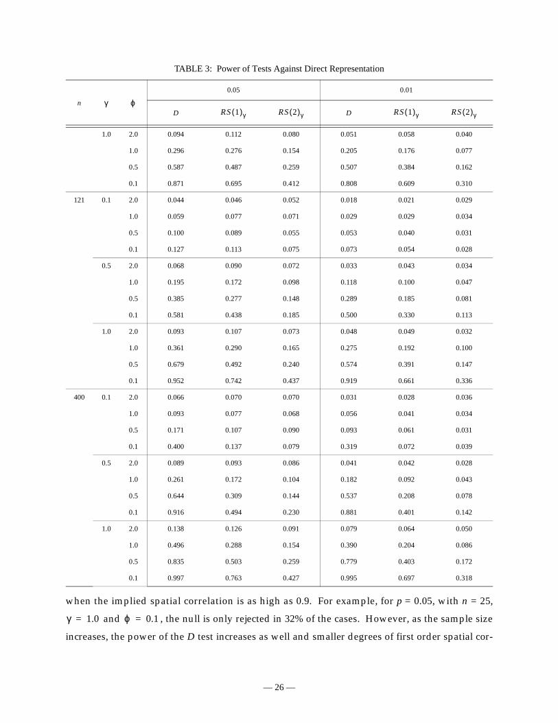
when the implied spatial correlation is as high as 0.9. For example, for p = 0.05, with n = 25,
and , the null is only rejected in 32% of the cases. However, as the sample size
increases, the power of the D test increases as well and smaller degrees of first order spatial cor-
1.0 2.0 0.094 0.112 0.080 0.051 0.058 0.040
1.0 0.296 0.276 0.154 0.205 0.176 0.077
0.5 0.587 0.487 0.259 0.507 0.384 0.162
0.1 0.871 0.695 0.412 0.808 0.609 0.310
121 0.1 2.0 0.044 0.046 0.052 0.018 0.021 0.029
1.0 0.059 0.077 0.071 0.029 0.029 0.034
0.5 0.100 0.089 0.055 0.053 0.040 0.031
0.1 0.127 0.113 0.075 0.073 0.054 0.028
0.5 2.0 0.068 0.090 0.072 0.033 0.043 0.034
1.0 0.195 0.172 0.098 0.118 0.100 0.047
0.5 0.385 0.277 0.148 0.289 0.185 0.081
0.1 0.581 0.438 0.185 0.500 0.330 0.113
1.0 2.0 0.093 0.107 0.073 0.048 0.049 0.032
1.0 0.361 0.290 0.165 0.275 0.192 0.100
0.5 0.679 0.492 0.240 0.574 0.391 0.147
0.1 0.952 0.742 0.437 0.919 0.661 0.336
400 0.1 2.0 0.066 0.070 0.070 0.031 0.028 0.036
1.0 0.093 0.077 0.068 0.056 0.041 0.034
0.5 0.171 0.107 0.090 0.093 0.061 0.031
0.1 0.400 0.137 0.079 0.319 0.072 0.039
0.5 2.0 0.089 0.093 0.086 0.041 0.042 0.028
1.0 0.261 0.172 0.104 0.182 0.092 0.043
0.5 0.644 0.309 0.144 0.537 0.208 0.078
0.1 0.916 0.494 0.230 0.881 0.401 0.142
1.0 2.0 0.138 0.126 0.091 0.079 0.064 0.050
1.0 0.496 0.288 0.154 0.390 0.204 0.086
0.5 0.835 0.503 0.259 0.779 0.403 0.172
0.1 0.997 0.763 0.427 0.995 0.697 0.318
TABLE 3: Power of Tests Against Direct Representation
n
0.05 0.01
D Dγ ϕ
RS 1( )γ RS 2( )γ RS 1( )γ RS 2( )γ
γ 1.0= ϕ 0.1=
— 27 —
relation are rejected in a majority of the cases. For n = 49 and n = 81, more than 50% rejection is
achieved for and (correlation > 0.6), with n = 121 for and (corre-
lation 0.48), and with n = 400, 40% rejection is already obtained for and , with an
implied first order spatial correlation of 0.10. For the highest degree of spatial correlation (0.9),
the D test yields rejection levels of 87% for n = 81, 95% for n = 121 and 99.7% for n = 400. This
seems to indicate that when the problem is severe, the D statistic properly detects it in even
medium-size samples. Further evidence is needed to assess its performance in non-standard sit-
uations, such as non-normal error distributions.
5. Concluding Remarks
The score test principle advanced in Rao’s (1947) classic paper has been shown to be par-
ticularly relevant in applications dealing with alternatives to the classic regression specification
that incorporate models of spatial dependence. For the three broad alternatives considered in
this paper, the RS test offers some significant advantages over other approaches.
When the alternative is in the form of a spatial autoregressive or moving average process,
the RS statistic is superior to the other classic testing principles in two important respects. The
first is computational, since the statistics can be constructed from the results of ordinary least
squares regression. The RS tests share this property with Moran’s I test and it turns out that both
are asymptotically equivalent. More importantly, the RS statistics (and particularly the form
robust to local misspecification) allow for the discrimination between alternatives in the form of
spatial lag dependence (Wy) and spatial error dependence (Wε). This is crucial both from an
inferential and from a substantive point of view, given the important differences between these
models.
The RS statistic also offers some important possibilities to tackle alternatives for spatial
dependence in the form of spatial error components and direct representation. The new statistics
derived in this paper avoid the problems associated with the failure to meet some regularity con-
ditions for maximum likelihood estimation. For spatial error components, the parameter value
under the null hypothesis is not an interior point of the parameter space. While Wald and Likeli-
hood Ratio statistics need to be adjusted to take into account the resulting censored nature of
their distribution, this is not the case for the RS statistic. For direct representation models, the sit-
uation is slightly more complex in that not only the parameter under the null is not an interior
point, but in addition the nuisance parameter is not identified under the null. This requires a
Davies-type adjustment to the RS statistic.
γ 1.0= ϕ 0.5< γ 0.5= ϕ 0.1=
γ 0.1= ϕ 0.1=
— 28 —
Both new tests that are outlined in this paper perform reasonably well in a limited series
of Monte Carlo simulation experiments. While they seem to be unreliable in small samples, for
data sets of more than a hundred observations they start to approach their asymptotic properties.
Given the increasingly common situation in practice where “spatial” data sets are large (with up
to thousands of observations), this is encouraging evidence for the practitioner. However, more
in depth study of the properties of these statistics in required, both in other contexts (non-normal
error distribution, presence of other forms of misspecification) as well as compared to some of
the recently suggested procedures that do not rely on the maximum likelihood paradigm.
In this paper, the discussion of Rao’s score principle has been limited to the classical lin-
ear regression model. Clearly, many other issues remain to be examined, such as extensions of
these approaches to the space-time domain and to models that incorporate limited dependent
variables. It is hoped that the review presented here will stimulate statisticians and econometri-
cians to tackle these interesting and challenging problems.
References
Anselin, L. (1980). Estimation methods for spatial autoregressive structures. Regional Science Dis-sertation and Monograph Series 8. Field of Regional Science, Cornell University, Ithaca, N.Y.
Anselin, L. (1988a). Spatial Econometrics: Methods and Models. Kluwer Academic, Dordrecht.Anselin, L. (1988b). Lagrange multiplier test diagnostics for spatial dependence and spatial het-
erogeneity. Geographical Analysis 20, 1–17.Anselin, L. (1990). Some robust approaches to testing and estimation in spatial econometrics.
Regional Science and Urban Economics 20, 141–163.Anselin, L. and A. Bera (1998). Spatial dependence in linear regression models with an introduc-
tion to spatial econometrics. In: A. Ullah and D. E. A. Giles, Eds., Handbook of Applied Eco-nomic Statistics. Marcel Dekker, New York, 237–289.
Anselin, L. and R. Florax (1995). Small sample properties of tests for spatial dependence inregression models: some further results. In: L. Anselin and R. Florax, Eds., New Directions inSpatial Econometrics. Springer-Verlag, Berlin, 21–74.
Anselin, L. and S. Hudak (1992). Spatial econometrics in practice, a review of software options.Regional Science and Urban Economics 22, 509–536.
Anselin, L. and H. H. Kelejian (1997). Testing for spatial error autocorrelation in the presence ofendogenous regressors. International Regional Science Review 20, 153–182.
Anselin, L. and R. Moreno (2000). Properties of tests for spatial error components. REAL Discus-sion Paper 00-T-12, University of Illinois, Urbana-Champaign.
Anselin, L. and S. Rey (1991). Properties of tests for spatial dependence in linear regression mod-els. Geographical Analysis 23, 112–131.
Anselin, L. and O. Smirnov (1996). Efficient algorithms for constructing proper higher order spa-tial lag operators. Journal of Regional Science 36, 67–89.
Anselin, L., A. Bera, R. Florax and M. Yoon (1996). Simple diagnostic tests for spatial depen-dence. Regional Science and Urban Economics 26, 77–104.
Andrews, D. W. K. and W. Ploberger (1994). Optimal tests when a nuisance parameter is presentonly under the alternative. Econometrica 62, 1383–1414.
Bera, A. and M. L. Higgins (1992). A test for conditional heteroskedasticity in time series models.
— 29 —
Journal of Time Series Analysis 13, 501–519.Bera, A. and S. Ra (1995). A test for the presence of conditional heteroskedasticity within ARCH-
M framework. Econometrics Reviews 14, 473–485.Bera, A., S. Ra and N. Sarkar (1996). Hypothesis testing for some nonregular cases in economet-
rics. In: S. Chakravarty, D. Coondoo and R. Mukherjee, Eds., Econometrics: Theory and Prac-tice. Allied Publishers, New Delhi, forthcoming.
Besag, J. (1974). Spatial interaction and the statistical analysis of lattice systems. Journal of theRoyal Statistical Society B 36, 192–225.
Blommestein, H. (1983). Specification and estimation of spatial econometric models: a discussionof alternative strategies for spatial economic modelling. Regional Science and Urban Economics13, 250–271.
Blommestein, H. (1985). Elimination of circular routes in spatial dynamic regression equations.Regional Science and Urban Economics 15, 121–130.
Box, G. E. P. and D. A. Pierce (1970). Distribution of residual autocorrelations in autoregressive-integrated moving average time series models. Journal of the American Statistical Association65, 1509–1526.
Brandsma, A.S. and R.H. Ketellapper (1979). A biparametric approach to spatial autocorrelation.Environment and Planning A 11, 51–58.
Breusch, T. (1980). Useful invariance results for generalized regression models. Journal of Econo-metrics 13, 327–340.
Burridge, P. (1980). On the Cliff-Ord test for spatial autocorrelation. Journal of the Royal StatisticalSociety B 42, 107–108.
Case, A. (1991). Spatial patterns in household demand. Econometrica 59, 953–965.Case, A., H.S. Rosen and J.R. Hines (1993). Budget spillovers and fiscal policy interdependence:
evidence from the States. Journal of Public Economics 52, 285–307.Chant, D. (1974). On asymptotic tests of composite hypotheses in non-standard conditions.
Biometrika 61, 291–299.Chernoff, H. (1954). On the distribution of the likelihood ratio. Annals of Mathematical Statistics
25, 573–578.Cliff, A. and J. K. Ord (1972). Testing for spatial autocorrelation among regression residuals.
Geographical Analysis 4, 267–284.Cliff, A. and J. K. Ord (1981). Spatial Processes: Models and Applications. Pion, London.Conley, T. G. (1996). Econometric modelling of cross-sectional dependence. Ph.D. Dissertation.
Department of Economics, University of Chicago, Chicago, IL.Cressie, N. (1993). Statistics for Spatial Data. Wiley, New York.Davies, R. B. (1977). Hypothesis testing when a nuisance parameter is present only under the
alternative. Biometrika 64, 247–254.Davies, R. B. (1987). Hypothesis testing when a nuisance parameter is present only under the
alternative. Biometrika 74, 33–43.Dubin, R. (1988). Estimation of regression coefficients in the presence of spatially autocorrelated
error terms. Review of Economics and Statistics 70, 466–474.Dubin, R. (1992). Spatial autocorrelation and neighborhood quality. Regional Science and Urban
Economics 22, 433–452.Godfrey, L. G. (1988). Misspecification tests in econometrics. Cambridge University Press, Cam-
bridge.Gouriéroux, C., A. Holly and A. Monfort (1982). Likelihood ratio test, Wald test, and Kuhn-
Tucker test in linear models with inequality constraints on the regression parameters. Econo-metrica 50, 63–80.
Haining, R. (1988). Estimating spatial means with an application to remotely sensed data. Com-munications in Statistics: Theory and Methods 17, 573–597.
— 30 —
Haining, R. (1990). Spatial Data Analysis in the Social and Environmental Sciences. Cambridge Uni-versity Press, Cambridge.
Hansen, B. E. (1996). Inference when a nuisance parameter is not identified under the nullhypothesis. Econometrica 64, 413–430.
Huang, J. S. (1984). The autoregressive moving average model for spatial analysis. AustralianJournal of Statistics 26, 169–178.
Kelejian, H. and I. Prucha (1998a). A generalized moments estimator for the autoregressiveparameter in a spatial model. International Economic Review (forthcoming).
Kelejian, H. and I. Prucha (1998b). A generalized spatial two stage least squares procedure forestimating a spatial autoregressive model with autoregressive disturbances. Journal of RealEstate Finance and Economics (forthcoming).
Kelejian, H. H. and D. P. Robinson (1993). A suggested method of estimation for spatial interde-pendent models with autocorrelated errors, and an application to a county expendituremodel. Papers in Regional Science 72, 297–312.
Kelejian, H. H. and D. P. Robinson (1995). Spatial correlation: a suggested alternative to theautoregressive model. In: L. Anselin and R. Florax, Eds., New Directions in Spatial Economet-rics. Springer-Verlag, Berlin, 75–95.
Kelejian, H. H. and D. P. Robinson (1997). Infrastructure productivity estimation and its under-lying econometric specifications: a sensitivity analysis. Papers in Regional Science 76, 115–131.
King, M. (1981). A small sample property of the Cliff-Ord test for spatial correlation. Journal ofthe Royal Statistical Society B 43, 263–264.
King, M. and T. S. Shively (1993). Locally optimal testing when a nuisance parameter is presentonly under the alternative. The Review of Economics and Statistics 75, 1–7.
Magnus, J. (1978). Maximum likelihood estimation of the GLS model with unknown parametersinthe disturbance covariance matrix. Journal of Econometrics 7, 281–312. (Corrigenda, Journal ofEconometrics 10, 261).
Mandy, D. M. and C. Martins-Filho (1994). A unified approach to asymptotic equivalence of Ait-ken and feasible Aitken instrumental variables estimators. International Economic Review 35,957–979.
Manski, C. F. (1993). Identification of endogenous social effects: the reflection problem. Review ofEconomic Studies 60, 531–542.
Mardia, K. V. (1990). Maximum likelihood estimation for spatial models. In: D. A. Griffith, Ed.,Spatial Statistics: Past, Present and Future. Institute of Mathematical Geography, Ann Arbor,MI, 203–251.
Mardia, K.V. and R.J. Marshall (1984). Maximum likelihood estimation of models for residualcovariance in spatial regression. Biometrika 71, 135–146.
Mardia, K.V. and A.J. Watkins (1989). On multimodality of the likelihood for the spatial linearmodel. Biometrika 76, 289–295.
Moran, P. A. P. (1948). The interpretation of statistical maps. Biometrika 35, 255–260.Moran, P. A. P. (1950a). Notes on continuous stochastic phenomena. Biometrika 37, 17–23.Moran, P. A. P. (1950b). A test for the serial dependence of residuals. Biometrika 37, 178–181.Moran, P. A. P. (1971). Maximum likelihood estimation in non-standard conditions. Proceedings
of the Cambridge Philosophical Society 70, 441–450.Olmo, J. C. (1995). Spatial estimation of housing prices and locational rents. Urban Studies 32,
1331–1344.Ord, J.K. (1975). Estimation methods for models of spatial interaction. Journal of the American Sta-
tistical Association 70, 120–126.Pace, R. K. (1997). Performing large spatial regressions and autoregressions. Economics Letters 54,
283–291.Pace, R. K. and R. Barry (1997). Sparse spatial autoregressions. Statistics and Probability Letters 33,
— 31 —
291–297.Paelinck, J. and L. Klaassen (1979). Spatial Econometrics. Saxon House, Farnborough.Pötscher, B.M. and I. R. Prucha (1997). Dynamic Nonlinear Econometric Models. Springer, Berlin.Rao, C. R. (1947). Large sample tests of statistical hypotheses concerning several parameters
with applications to problems of estimation. Proceedings of Cambridge Philosophical Society 44,50–57.
Rao, C. R. (1973). Linear Statistical Inference and its Applications (2nd Ed.). Wiley, New York.Ripley, B. D. (1981). Spatial Statistics. Wiley, New York.Serfling, R. J. (1980). Approximation Theorems of Mathematical Statistics. Wiley, New York.Silvey, S. D. (1959). The Lagrange multiplier test. Annals of Mathematical Statistics 30, 387–407.Upton, G. J. and B. Fingleton (1985). Spatial Data Analysis by Example. Volume 1: Point Pattern and
Quantitative Data. Wiley, New York.Warnes, J.J. and B.D. Ripley (1987). Problems with likelihood estimation of covariance functions
of spatial Gaussian processes. Biometrika 74, 640–642.White, H. (1984). Asymptotic Theory for Econometricians. Academic Press, Orlando.Whittle, P. (1954). On stationary processes in the plane. Biometrika 41, 434–449.