1

Mostly Pointless Spatial Econometrics?1

Steve Gibbons (SERC and LSE)2

Henry Overman (SERC and LSE)3

Abstract: We argue that identification problems bedevil applied spatial economic research. Spatial

econometrics usually solves these problems by deriving estimators assuming that functional forms

are known and by using model comparison techniques to let the data choose between competing

specifications. We argue that in many situations of interest this, at best, achieves only very weak

identification. Worse, in many cases, such an approach will be uninformative about the causal

economic processes at work, rendering much applied spatial econometric research ‘pointless’,

unless the main aim is description of the data. We advocate an alternative approach based on the

‘experimental paradigm’ which puts issues of identification and causality at centre stage.

1 The title is a reference to Angrist and Pischke’s (2009) “Mostly Harmless Econometrics” which outlines the

experimental paradigm and argues that fancier econometric techniques are unnecessary and potentially

dangerous.

2 Steve Gibbons, Spatial Economics Research Centre and Department of Geography and Environment, London

School of Economics, Houghton Street, London, WC2A 2AE, UK. Email: s.gibbons@lse.ac.uk .

3 Henry G. Overman, Spatial Economics Research Centre and Department of Geography and Environment,

London School of Economics, Houghton Street, London, WC2A 2AE, UK. Email: h.g.overman@lse.ac.uk .

2

1. INTRODUCTION

The last two decades have seen economists become increasingly interested in geographical issues

(Martin, 1999, Behrens and Robert-Nicoud, 2009). This has been variously attributed to theoretical

developments (the New Economic Geography), a growing interest in cities (the expansion of urban

economics) or simply the greater availability of geo-referenced data (Overman, 2010). Regardless of

the reason, the upshot has been greater interaction between economic geographers, regional

scientists and economists in an attempt to understand spatial aspects of the economy. More

recently, a similar process has seen mainstream econometric theorists becoming increasingly

interested in spatial processes, traditionally the preserve of a specialised group of spatial

econometricians.4 One might think that the next step would be convergence between the tools

developed by spatial econometricians and the methods used by applied economists to assess the

extent to which models of spatial economics explain real world data. We argue that this is unlikely to

happen because, while there may have been convergence between mainstream and spatial

econometric theory, most applied economic research is taking a different path.

In many (micro) economic fields – particularly in development, education, environment, labor,

health, and public finance – empirical work is increasingly concerned with answering questions

about causal relationships (Angrist & Pischke, 2010). If we increase an individual’s years of

education, what happens to their wages? If we decrease class sizes, what happens to student

grades? These questions are fundamentally of the type “if we change x, what do we expect to

happen to y”. Just as with economics more generally, answering such questions is fundamental to

increasing our understanding of spatial economics. When more skilled people live in an area, what

do we expect to happen to individual wages? If a jurisdiction increases taxes, what do we expect to

happen to taxes in neighbouring jurisdictions?

In an experimental setting, agents (individuals, firms, governments) would be randomly assigned

different amounts of x and the outcomes y observed. Measuring whether different levels of x are

associated with different outcomes would then give us the causal effect of x on y. The fundamental

challenge to answering these types of questions for (most) economic data is that we do not

randomly assign x and observe outcomes y. Instead, we jointly observe x and y so we lack the

counterfactual as to what would have happened if we were to change x. Fortunately, applied

economics has come a long way in its efforts to find credible and creative ways to answer such

questions by constructing counterfactuals from observational data.

A good starting point for thinking about whether a particular question about causality can be

answered and how to answer it, is to consider what an ideal experiment might look like. The

experiment may not be feasible, but with the design in mind it is easier to think of ways to find

sources of variation in the data that mimic or approximate the conditions of the ideal experiment.

The ‘experimental paradigm’ (Angrist and Pischke, 2009, 2010) does this by using simple linear

4 See Anselin (2010) who argues that the last 30 years have seen spatial econometrics move from the margins

to the mainstream of econometrics and social science methodology. Many of the specialised econometricians

who helped developed the field are recognised by Fellowship of the Spatial Econometric Association. See the

list at http://spatialeconometr.altervista.org/?Fellows_of_the_association.

3

estimation methods, taking care to pinpoint and isolate sources of variation in x that can plausibly be

considered exogenous to y. The aim of these methods is to mimic, as far as possible, the conditions

of an experiment in which agents are randomly assigned different amounts of x and outcomes y

observed. The central idea is to find otherwise comparable agents (e.g. twins, siblings, neighbours,

school-mates, cities, regions) who for some reason have been exposed to different amounts of x.

This approach is still 'econometric' in that it draws on economic theory to guide the questions being

asked and the thinking about what causal processes are at work. However, the fundamental

attraction is that the assumptions required for identification of causal effects are usually clearly

specified and understandable without reference to specific (and untested) economic theories. Put

another way, the aim is to obtain plausible estimates of causal effects without relying on specific ad-

hoc functional forms and exclusion restrictions imposed arbitrarily by the econometrician, or derived

from untested theories about which there is no consensus.5 This approach is particularly attractive

in areas, like much of spatial economics, where we are far from having a structural model that

closely captures the complexities that drive the processes for which we observe data.6

Unfortunately, although these issues may be well understood by more experienced practitioners,

they are not widely discussed in many of the ‘standard’ spatial econometrics references. 7 For this

reason there is a danger that people entering the world of applied economic research using spatial

econometrics will ignore these insights into framing research questions and arriving at credible

research designs.

Why is it the case that the spatial econometrics literature usually ignores these issues? An important

part of the answer, we suspect, is because the underlying theory has developed from time-series

foundations, in such a way that questions about causality have never been centre stage. The

standard approach to spatial econometrics has been to write down one of a number of spatial model

specifications (e.g. the spatial autoregressive model), to assume that the equation accurately

describes the data generating processes (usually without any strong behavioural foundations), and

then to estimate the parameters by non-linear methods such as (quasi) maximum likelihood (ML).

Because estimation is not always simple, much effort has gone in to developing techniques that

allow estimation of parameters from a range of models for large data sets. Questions of

identification (i.e. does an estimated correlation imply that x causes y?) have been addressed by

5 The assumption of linearity and the reliance on simple linear methods may appear like quite a strong

functional form assumption. However, as Angrist and Pischke 2009 (p.69) argue, the assumption of a linear

structural relationship - the Conditional Expectation Function (CEF) - is “not really necessary for a causal

interpretation of regression”. If the CEF is causal then, because the linear regression provides the best linear

approximation to the CEF, the regression coefficients are informative about causality.

6 Sutton (2002) makes a similar argument about the use of structural modelling in situations where models are

‘far from reality’. Later in the paper we will briefly discuss the use of spatial econometrics in facilitating the

estimation of structural econometric models. This is not to say that we claim theoretical structure has no place

in empirical spatial economics. There are situations, particularly when general equilibrium considerations are

important, when there can be a greater role for assuming a theoretical model that is solidly grounded in

micro-economic behavioural foundations. See Combes, Duranton and Gobillon (2011) for further discussion.

7 For example, there is little, if any discussion of these issues in the two recent text books by Arbia (2006) and

LeSage and Pace (2009).

4

asking which of these assumed spatial processes best fit the data. While in principle this sounds

straightforward, in practice, as we discuss further below, it is hard to distinguish between alternative

specifications that have very different implications for which causal relationships are at work.

In this article we explain why the standard spatial econometric toolbox is unlikely to offer a solution

to the problem of the identification of causal effects in many spatial economic settings. Of course,

much standard (i.e. non-spatial) empirical economic analysis falls someway short of the lofty ideals

of identifying causal effects from random variation in the variable of interest (x). Finding sources of

truly exogenous or random variation in x is difficult, but good applied work aimed at causal analysis

must surely make some credible attempt to do so. This is not to say that non-causal associations are

never without merit, because description and correlation can provide essential insights into the

problem at hand. However, identification of causal effects remains the gold standard to which many

economists claim to aspire. We will argue that this should also be the case in applied spatial

economic research.

The rest of this paper is structured as follows. Section 2 provides a basic overview of standard spatial

econometric models, while section 3 discusses problems of identification. Section 4 returns to the

relationship between the spatial econometrics and experimental paradigms. Section 5 concludes.

2. SPATIAL ECONOMETRIC MODELS AND THEIR MOTIVATION

This section provides an introduction to spatial econometric models, of the type popularised by the

seminal work of Anselin (1988). It is not comprehensive but provides enough background so that

someone unfamiliar with spatial econometrics should be able to follow the arguments made later.

We generally use the model terminology of LeSage and Pace (2009) and refer the reader there for

details.

To develop ideas, start with a basic linear regression:

'i i iy u= +x β (1)

where i indexes units of observation, iy is the outcome of interest, ix is a vector of explanatory

variables, iu is an error term and β is a vector of parameters.8 In the most basic regression

specification it is assumed that outcomes for different units are independent of each other. This is a

strong assumption and there may be many reasons why outcomes are not independent, particularly

when observations are for geographically referenced events, agents or places. In short, in a spatial

setting, this model is often not very interesting. There are many contexts in which estimating and

interpreting the parameters that characterise this dependence, which may imply interaction

between agents or other spatial units, is of academic and policy interest.

Estimating the complete between-observation variance-covariance structure is infeasible. However,

if the data are spatial, i.e. can be mapped to locations, relative positions (and possibly direction) may

restrict the connections between observations. For example, outcomes at a given location may

8 For ease of exposition we subsume the constant in

'ix β .

5

depend on outcomes in ‘nearby’ locations but not those further away. A simple way to capture these

restrictions on the spatial connections between observations is to define a vector iw where the jth

element takes a value that is bigger, the more closely connected j is with i (e.g. 1/ distanceij ). If we

have n observations, then multiplying 'iw by the nx1 vector of outcomes y gives us a value '

iw y

that spatial econometricians refer to as a spatial lag. For each observation, 'iw y is a linear

combination of all jy with which the ith observation is connected. If, as is usually the case, we

normalise iw so that the elements sum to 1, then 'iw y is a weighted average of the 'neighbours' of

i.

What now if we want to understand whether changes in the outcome iy are related to changes in

outcomes at the locations to which i is connected? A simple solution, proposed by Ord (1975) is to

assume that effect of the spatial lag of iy on iy is linear, with a parameter ρ that is constant across

observations. This gives the spatial autoregressive model (SAR):

' 'i i i iy uρ= + +w y x β (SAR)

LeSage and Pace (2009) suggest a “time dependence motivation” for the SAR model. Assume fixed

across time exogenous variables ix determine outcome iy . Now assume that when determining

their own outcome, agents take in to account both their own characteristics and recent outcomes

for other ‘nearby’ agents. We might think of iy as the price of a house, ix as the fixed

characteristics (number of rooms) and assume that when agreeing a sale price, people consider both

the characteristics of the house and the current selling price of nearby houses. In this case β

captures the causal effect of house characteristics and ρ represents the causal effect of neighbouring

prices (conditional on observed housing characteristics).

We could drop the assumption that iy is affected by the spatial lag of iy and instead assume that

iy is affected by spatial lags of the explanatory variables. If X denotes the matrix of explanatory

variables and γ a vector of parameters, this gives the spatial (lag of) X model (SLX):

' 'i i i iy u= + +x β w Xγ (SLX)

LeSage and Pace (2009) provide an ‘externality motivation’ for this model. Assume that the

exogenous characteristics of nearby observations directly affect iy . Continuing with the housing

example, this assumes the characteristics of nearby houses, e.g. their size, directly determine prices

(rather than working through observed sales prices). Of course, an externality motivation could also

justify the SAR model if the externality works through the spatial lag of iy

Next, drop the assumption that the dependent variable is affected by spatial lags of the explanatory

variables and instead assume spatial autocorrelation in the error process. The SAR process can be

6

used to place structure on this process.9 If u denotes the vector of residuals, this gives the spatial

error model (SE):

' ';i i i i i iy u u vρ= + = +x β w u (SE)

Finally, combining the SAR and SLX models gives us the Spatial Durbin Model (SD):

' ' 'i i i i iy uρ= + + +w y x β w Xγ (SD)

which assumes dependence between iy and the spatial lags of both the outcome and explanatory

variables, but drops the assumption of spatial autocorrelation in the error process.

The SD model can be motivated by a combination of the arguments above (causal effects from

neighbouring outcomes and neighbouring characteristics). Alternatively, it can be motivated by

simply re-arranging the SE model in a spatial Cochrane-Orcutt style transformation:

'i i iu y= − x β (2)

' ' 'i i i i iy vρ ρ− = − +x β w y w Xβ (3)

' ' 'i i i i iy vρ ρ= + − +w y x β w Xβ (4)

An extension to this idea provides another motivation for including spatial lags of y and X, as a

solution to the omitted variables problem. Assume iy depends on an exogenous variable ( ix ) and

unobservable factors ( iz ). That is, the true model is:

i i iy x zβ= + (5)

Further, assume that the unobservable iz is both spatially correlated and partly determined by ix ,

such that:

'i i i iz w x vρ γ= + +z (6)

substituting i i iz y x β= − into (6) and rearranging gives

' '( )i i i i iy x vρ γ β ρ= + + − +w y w xβ (7)

From (4) and (7) note that the presence of a spatially correlated error term, whether correlated with

ix or not, leads to the SD model involving a spatial lag in y and X. It is important to emphasise,

however, that in this motivation for the SD model, ρ cannot be interpreted as revealing anything

about the causal effect of spatial lags of y or X on outcomes. The spatial lags of y and X are simply

being used to control for spatial correlation in the error term. This hints at the problems of

identification in spatial models that we discuss further below.

9 More general specifications are available, but the SE model defined in the text is sufficient for our purposes.

7

These five processes are not exhaustive of all possible models, and we consider a particularly

important generalisation further below, but for the moment they are sufficient for our purposes. In

the text, we use the acronyms (SAR, etc) to refer to the specifications above.

Estimation using OLS gives inconsistent parameter estimates if the models include a spatially lagged

dependent variable and ρ is non-zero (e.g. the SAR and SD models). This inconsistency arises

because of a mechanical link between iu and 'iw y for most specifications of iw . Standard errors

are also inconsistently estimated for these models, as well as for models including a spatial lag in the

error term (e.g. the SE model). OLS provides consistent estimates of the parameters if the spatial

correlation occurs only through the error term (SE model) or exogenous characteristics (SLX model).

In both cases standard errors are inconsistent, and OLS estimation of the SE model is inefficient. In

contrast, Lee (2004) shows that (quasi) ML estimation provides consistent estimators for all these

models conditional on the assumption that the spatial econometric model estimated is the true data

generating process. Alongside theoretical developments, advances in computational power and

methods have made ML estimation feasible for large datasets.10 As a result, ML estimation is

preferred in the spatial econometrics literature. Inspection of the SAR and SLX models reveals they

are nested within the SD model. We have also shown that the SE model can be rearranged to give

the SD model. The fact that the SD model nests many of the other models provides an argument for

estimating the SD model and then testing this against the nested models through the use of

likelihood tests. This is the approach advocated by LeSage and Pace (2009). Model comparison

techniques can be used to compare models based on different weight matrices and explanatory

variables.

We have shown that contrasting motivations lead to different spatial econometric models. This

suggests we might learn about the underlying processes at work if we use ML estimation and model

comparison to find the correct specification for given data. Unfortunately, as we show in the next

section, these different specifications will generally be impossible to distinguish without assuming

prior knowledge about the true data generating process that we often do not possess in practice. In

short, contrasting motivations lead to spatial econometrics models that cannot usually be easily

distinguished in applied research.

It is useful to see how these models are related to each other. Consider the reduced form (which

expresses iy in terms of exogenous factors) of the SAR model. If the model is correct, the only

exogenous factors affecting iy are ix and iu , so the only factors affecting 'iw y (the spatial lag of

iy ) are 'iw X and '

iw u (the spatial lags of X and u , respectively). The spatial lag of iy ( 'iw y ) also

depends on the second order spatial lag of iy ( 'iw Wy ), that is, on outcomes for the “neighbours of

my neighbours”. By repeated substitution (first for 'iw y , then for '

iw Wy etc), the reduced form is:

' ' 2 ' 3 ' 2[ ]i i i i i iy vρ ρ ρ= + + + + +x β w Xβ w WXβ w W Xβ … (8)

10 According to LeSage and Pace (2009, p.45) “these improvements allow models involving samples containing

more than 60,000 US Census tract observations to be estimated in only a few seconds on desktop and laptop

computers”

8

where 'i i iv uρ= +w v , W is the matrix of stacked weight vectors ( '

iw ) and 2 =W WW .

Notice that, in the reduced form, the only thing that distinguishes this from the SLX model is the

absence of terms in ' 1n niρ −

w W Xγ for n>1. As we explain in the next section, in practice these two

models will often be hard to tell apart even if, technically, both are identified. This similarity is

problematic, because the models have different implications for the economic processes at work.

It is also informative to derive the reduced form for the general SD model. Substituting for y we get:

' ' '

2 ' ' ' ' '

2 ' ' ' '

' 1 ' ' ' 2 ' 2

( )

( )

[ ]

( ) ( ) ( ) [ ]

i i i i i

i i i i i i

i i i i i

n ni i i i i i

y u

v

v

v

ρ ρ

ρ ρ ρ

ρ ρ ρ

ρ ρ ρ ρ ρ ρ−

= + + + + + +

= + + + + +

= + + + + +

=

= + + + + + + + + +

w Wy Xβ WXγ u x β w Xγ

w Wy w Xβ w WXγ x β w Xγ

w Wy x β w X β γ w WXγ

w W y x β w X β γ w WX β γ w W X β γ

…

…

(9)

where iv denotes the spatial lag terms in iu . Under standard regularity conditions on ρ and iw , ' 1

lim 0n n

n iρ −→∞ =w W y so the spatially lagged term in y can be ignored. Notice that, in the reduced

form, the only thing that distinguishes this from the SLX model is the cross coefficient restrictions on

the terms in ' 1ni

−w W X for n>1.

In short, spatial interaction in iy , spatial externalities in ix , or spatially omitted variables lead to

different spatial econometric specifications. However, the reduced form for all these models is:

' ' ' ' 21 2 3 [ ]i i i i i iy v= + + + + +x β w Xπ w WXπ w W Xπ … (10)

and the only differences arise from how many spatial lags of ix are included, constraints on the way

the underlying parameters determine the composite parameters Π , and whether the error term is

spatially correlated. Distinguishing which of these models generates the data that the researcher has

at hand is going to be difficult. This is the case, because the specification of W is (in most situations)

arbitrary, and because the spatial lags of ix are just neighbour averages that are almost always very

highly mutually correlated. We now consider these difficulties in detail.

3. THE REFLECTION PROBLEM AND CRITIQUE OF SPATIAL

ECONOMETRIC MODELS

Readers familiar with the ‘neighbourhood effects’ literature, will see immediate parallels between

the spatial econometrics models (SAR, etc) and ‘linear-in-means’ neighbourhood effects models that

appear in many branches of applied economics.11 The parallels between these fields have already

been highlighted by Lee (2004, 2007) and others. The generic neighbourhood effects model

described by Manski (1993, 2000) and used by countless applied economics papers on

neighbourhood effects since, takes the form:

11 The points we make here apply equally to the peer effects literature.

9

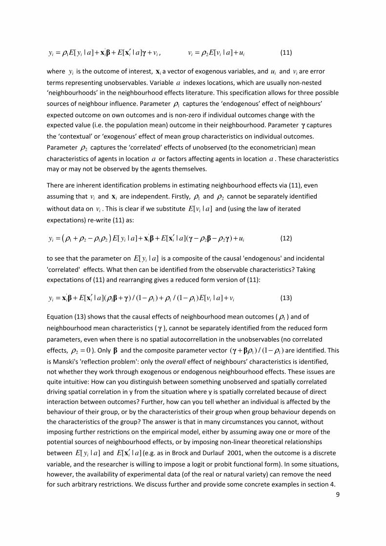
'1 [ | ] [ | ]i i i i iy E y a E a vρ ′= + + +x β x γ , 2 [ | ]i i iv E v a uρ= + (11)

where iy is the outcome of interest, ix a vector of exogenous variables, and iu and iv are error

terms representing unobservables. Variable a indexes locations, which are usually non-nested

‘neighbourhoods’ in the neighbourhood effects literature. This specification allows for three possible

sources of neighbour influence. Parameter 1ρ captures the ‘endogenous’ effect of neighbours’

expected outcome on own outcomes and is non-zero if individual outcomes change with the

expected value (i.e. the population mean) outcome in their neighbourhood. Parameter γ captures

the ‘contextual’ or ‘exogenous’ effect of mean group characteristics on individual outcomes.

Parameter 2ρ captures the ‘correlated’ effects of unobserved (to the econometrician) mean

characteristics of agents in location a or factors affecting agents in location a . These characteristics

may or may not be observed by the agents themselves.

There are inherent identification problems in estimating neighbourhood effects via (11), even

assuming that iv and ix are independent. Firstly, 1ρ and 2ρ cannot be separately identified

without data on iv . This is clear if we substitute [ | ]iE v a and (using the law of iterated

expectations) re-write (11) as:

( ) '1 2 1 2 2 2[ | ] [ | ]( )i i i i iy E y a E a uρ ρ ρ ρ ρ ρ′= + − + + − − +x β x γ β γ (12)

to see that the parameter on [ | ]iE y a is a composite of the causal 'endogenous' and incidental

'correlated' effects. What then can be identified from the observable characteristics? Taking

expectations of (11) and rearranging gives a reduced form version of (11):

'1 1 1 1[ | ]( ) / (1 ) / (1 ) [ | ]i i i i iy E a E v a vρ ρ ρ ρ′= + + − + − +x β x β γ (13)

Equation (13) shows that the causal effects of neighbourhood mean outcomes ( 1ρ ) and of

neighbourhood mean characteristics ( γ ), cannot be separately identified from the reduced form

parameters, even when there is no spatial autocorrellation in the unobservables (no correlated

effects, 2 0ρ = ). Only β and the composite parameter vector 1 1( ) / (1 )ρ ρ+ −γ β are identified. This

is Manski's 'reflection problem': only the overall effect of neighbours’ characteristics is identified,

not whether they work through exogenous or endogenous neighbourhood effects. These issues are

quite intuitive: How can you distinguish between something unobserved and spatially correlated

driving spatial correlation in y from the situation where y is spatially correlated because of direct

interaction between outcomes? Further, how can you tell whether an individual is affected by the

behaviour of their group, or by the characteristics of their group when group behaviour depends on

the characteristics of the group? The answer is that in many circumstances you cannot, without

imposing further restrictions on the empirical model, either by assuming away one or more of the

potential sources of neighbourhood effects, or by imposing non-linear theoretical relationships

between [ | ]iE y a and [ | ]iE a′x (e.g. as in Brock and Durlauf 2001, when the outcome is a discrete

variable, and the researcher is willing to impose a logit or probit functional form). In some situations,

however, the availability of experimental data (of the real or natural variety) can remove the need

for such arbitrary restrictions. We discuss further and provide some concrete examples in section 4.

10

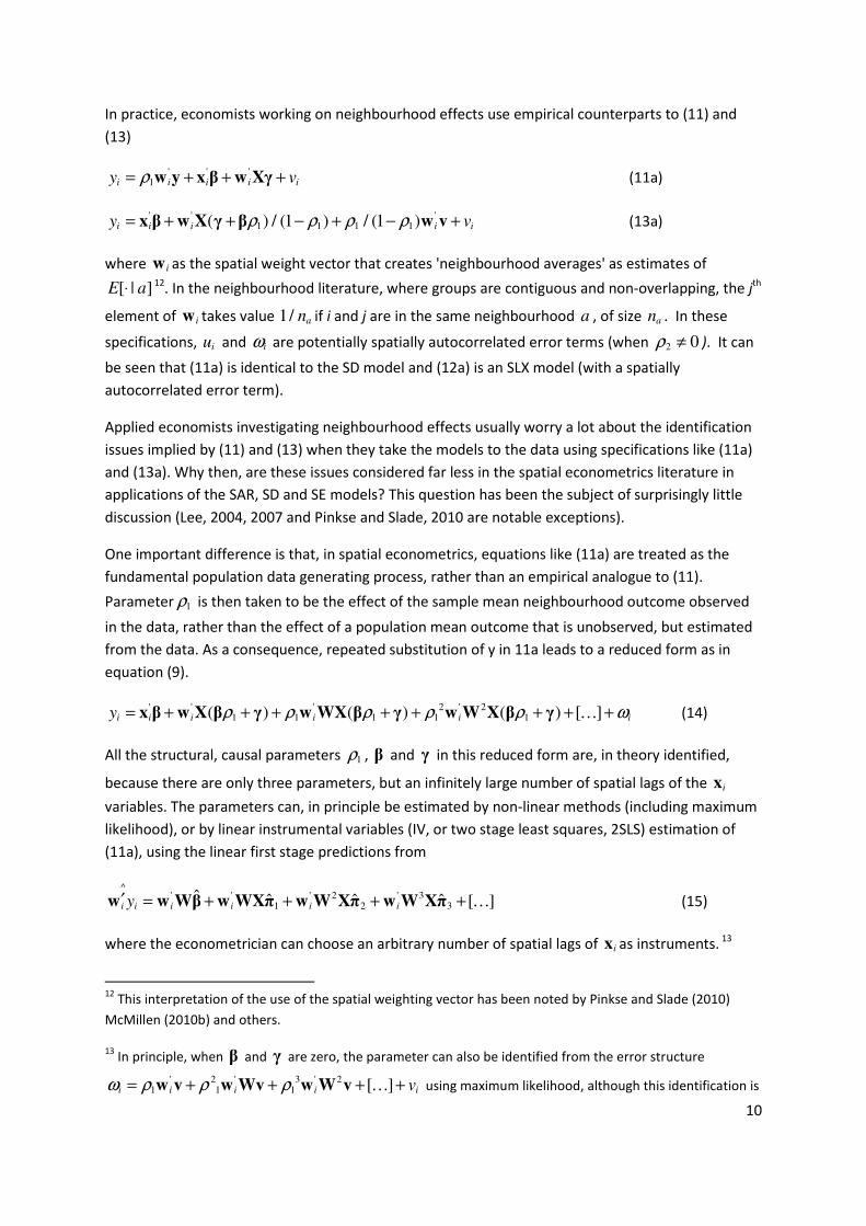
In practice, economists working on neighbourhood effects use empirical counterparts to (11) and

(13)

' ' '1i i i i iy vρ= + + +w y x β w Xγ (11a)

' ' '1 1 1 1( ) / (1 ) / (1 )i i i i iy vρ ρ ρ ρ= + + − + − +x β w X γ β w v (13a)

where iw as the spatial weight vector that creates 'neighbourhood averages' as estimates of

[ | ]E a⋅ 12. In the neighbourhood literature, where groups are contiguous and non-overlapping, the jth

element of iw takes value 1/ an if i and j are in the same neighbourhood a , of size an . In these

specifications, iu and iω are potentially spatially autocorrelated error terms (when 2 0ρ ≠ ). It can

be seen that (11a) is identical to the SD model and (12a) is an SLX model (with a spatially

autocorrelated error term).

Applied economists investigating neighbourhood effects usually worry a lot about the identification

issues implied by (11) and (13) when they take the models to the data using specifications like (11a)

and (13a). Why then, are these issues considered far less in the spatial econometrics literature in

applications of the SAR, SD and SE models? This question has been the subject of surprisingly little

discussion (Lee, 2004, 2007 and Pinkse and Slade, 2010 are notable exceptions).

One important difference is that, in spatial econometrics, equations like (11a) are treated as the

fundamental population data generating process, rather than an empirical analogue to (11).

Parameter 1ρ is then taken to be the effect of the sample mean neighbourhood outcome observed

in the data, rather than the effect of a population mean outcome that is unobserved, but estimated

from the data. As a consequence, repeated substitution of y in 11a leads to a reduced form as in

equation (9).

' ' ' 2 ' 21 1 1 1 1( ) ( ) ( ) [ ]i i i i i iy ρ ρ ρ ρ ρ ω= + + + + + + + +x β w X β γ w WX β γ w W X β γ … (14)

All the structural, causal parameters 1ρ , β and γ in this reduced form are, in theory identified,

because there are only three parameters, but an infinitely large number of spatial lags of the ix

variables. The parameters can, in principle be estimated by non-linear methods (including maximum

likelihood), or by linear instrumental variables (IV, or two stage least squares, 2SLS) estimation of

(11a), using the linear first stage predictions from

^' ' ' 2 ' 3

1 2 3ˆ ˆ ˆ ˆ [ ]i i i i i iy′ = + + + +w w Wβ w WXπ w W Xπ w W Xπ … (15)

where the econometrician can choose an arbitrary number of spatial lags of ix as instruments. 13

12 This interpretation of the use of the spatial weighting vector has been noted by Pinkse and Slade (2010)

McMillen (2010b) and others.

13 In principle, when β and γ are zero, the parameter can also be identified from the error structure

' 2 ' 3 ' 21 1 1 [ ]i i i i ivω ρ ρ ρ= + + + +w v w Wv w W v … using maximum likelihood, although this identification is

11

So why do spatial econometricians argue that (11a) is identified, by virtue of (14), when other

economists working on neighbourhood effects would argue that (11a) isn't identified, by virtue of

(13a)? The crucial difference is that spatial econometrics methods assume that W is known with

certainty and represents a system of real-world linkages between agents or places. Neighbourhood

effects researchers would argue that the true W is almost never known or observed, and is, at best,

a means of estimating [ | ]E a⋅ . In other words, the assumption of knowledge about W is critical. 14

This is easily seen in that if W takes the typical block-diagonal structure used in neighbourhood

effects studies (or W is otherwise idempotent) then (14) collapses to (13a) and the parameters are

no longer separately identified.

Even if W is not idempotent, there are serious problems in relying on (14) and (15) for

identification of the parameters in (11a). Firstly if the exact structure of W is not known – i.e it is

not known exactly which neighbours matter – then identification breaks down because 'iw W ,

' 2iw W etc. may better capture the connections between observation i and its neighbours than does

iw (e.g. ix has an effect up to 5km, but iw incorrectly restricts effects to within 2km) . If the higher

order lags 'iw WX , ' 2

iw W X affect y directly, then they cannot provide additional information to

identify 1ρ . It is easiest to think about this in the context of the linear (2SLS) IV estimator implicit in

(14) and (15) ( e.g. Kelejian and Prucha 1998): If the exclusion restrictions on 'iw WX , ' 2

iw W X etc.

in (11a) are not appropriate, then these spatial lag variables are unsuitable as instruments, nor as

sources of identification more generally.

Secondly, even if the structure of W is assumed to be known (and W is not idempotent) there are

serious practical estimation problems in that the spatial lag variables 'iw X '

iw WX , ' 2iw W X etc.

are likely to be very highly correlated. This collinearity implies that the reduced form coefficients in

(14), and hence the structural parameters, are likely to be imprecisely estimated. In the IV context,

there is a ‘weak instruments’/ ‘weak identification’ problem, in which there is little independent

variation and hence little additional information in the higher order spatial lags of ix , conditional on 'iw X . Since Bound, Jaeger and Baker (1995) and Staiger and Stock (1997), applied researchers have

worried about the strength of the instruments in IV regressions, because weak instruments can lead

second stage coefficient estimates to be biased and imprecisely estimated (Stock, Wright and Yogo

2002). As before, the variables 'iw X '

iw WX , ' 2iw W X are therefore potentially of little practical

use as sources of identification. This issue has certainly been recognised in the spatial econometrics

literature but the profound consequences do not appear to have had much influence on the applied

literature.

clearly purely parametric in the sense that it relies on the empirical model being an exact representation of

the data generating process.

14 Interestingly, the idea of putting more structure on neighbourhood effects (e.g. by assuming a hierarchical

network) has recently been suggested as a way of solving the identification problem. See Lee at al (2010).

12

In theory, the degree of collinearity between spatial lags depends on sample size, sampling frame

and how W changes as observations are added.15 In practice, in large samples (and using standard

iw ), 'iw X , '

iw WX , etc are likely to be highly correlated for the simple reason that they are a

weighted average (and consistent estimates of the mean) of ix in some neighbourhood of i. As a

result in many applications the parameters on 'iw X , '

iw WX , etc are likely to be imprecisely

measured and/or biased.

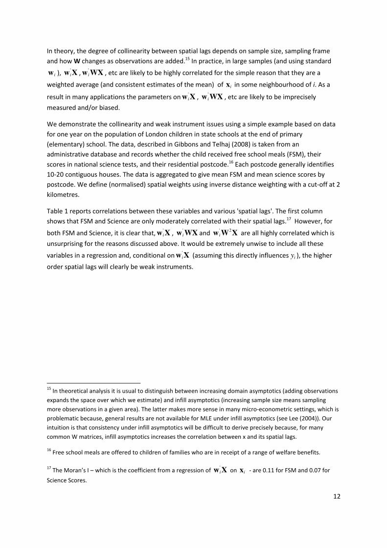
We demonstrate the collinearity and weak instrument issues using a simple example based on data

for one year on the population of London children in state schools at the end of primary

(elementary) school. The data, described in Gibbons and Telhaj (2008) is taken from an

administrative database and records whether the child received free school meals (FSM), their

scores in national science tests, and their residential postcode.16 Each postcode generally identifies

10-20 contiguous houses. The data is aggregated to give mean FSM and mean science scores by

postcode. We define (normalised) spatial weights using inverse distance weighting with a cut-off at 2

kilometres.

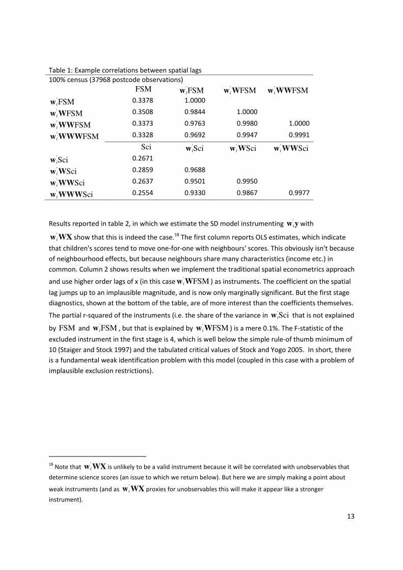
Table 1 reports correlations between these variables and various 'spatial lags'. The first column

shows that FSM and Science are only moderately correlated with their spatial lags.17 However, for

both FSM and Science, it is clear that, 'iw X , '

iw WX and ' 2iw W X are all highly correlated which is

unsurprising for the reasons discussed above. It would be extremely unwise to include all these

variables in a regression and, conditional on 'iw X (assuming this directly influences iy ), the higher

order spatial lags will clearly be weak instruments.

15 In theoretical analysis it is usual to distinguish between increasing domain asymptotics (adding observations

expands the space over which we estimate) and infill asymptotics (increasing sample size means sampling

more observations in a given area). The latter makes more sense in many micro-econometric settings, which is

problematic because, general results are not available for MLE under infill asymptotics (see Lee (2004)). Our

intuition is that consistency under infill asymptotics will be difficult to derive precisely because, for many

common W matrices, infill asymptotics increases the correlation between x and its spatial lags.

16 Free school meals are offered to children of families who are in receipt of a range of welfare benefits.

17 The Moran’s I – which is the coefficient from a regression of 'iw X on ix - are 0.11 for FSM and 0.07 for

Science Scores.

13

Table 1: Example correlations between spatial lags 100% census (37968 postcode observations) FSM '

FSMiw 'FSMiw W '

FSMiw WW 'FSMiw 0.3378 1.0000

'FSMiw W 0.3508 0.9844 1.0000

'FSMiw WW 0.3373 0.9763 0.9980 1.0000

'FSMiw WWW 0.3328 0.9692 0.9947 0.9991

Sci 'Sciiw '

Sciiw W 'Sciiw WW

'Sciiw 0.2671

'Sciiw W 0.2859 0.9688

'Sciiw WW 0.2637 0.9501 0.9950

'Sciiw WWW 0.2554 0.9330 0.9867 0.9977

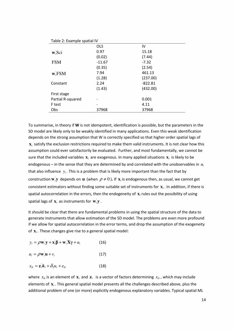
Results reported in table 2, in which we estimate the SD model instrumenting 'iw y with

'iw WX show that this is indeed the case.18 The first column reports OLS estimates, which indicate

that children's scores tend to move one-for-one with neighbours' scores. This obviously isn't because

of neighbourhood effects, but because neighbours share many characteristics (income etc.) in

common. Column 2 shows results when we implement the traditional spatial econometrics approach

and use higher order lags of x (in this case 'FSMiw W ) as instruments. The coefficient on the spatial

lag jumps up to an implausible magnitude, and is now only marginally significant. But the first stage

diagnostics, shown at the bottom of the table, are of more interest than the coefficients themselves.

The partial r-squared of the instruments (i.e. the share of the variance in 'Sciiw that is not explained

by FSM and 'FSMiw , but that is explained by '

FSMiw W ) is a mere 0.1%. The F-statistic of the

excluded instrument in the first stage is 4, which is well below the simple rule-of thumb minimum of

10 (Staiger and Stock 1997) and the tabulated critical values of Stock and Yogo 2005. In short, there

is a fundamental weak identification problem with this model (coupled in this case with a problem of

implausible exclusion restrictions).

18 Note that

'iw WX is unlikely to be a valid instrument because it will be correlated with unobservables that

determine science scores (an issue to which we return below). But here we are simply making a point about

weak instruments (and as 'iw WX proxies for unobservables this will make it appear like a stronger

instrument).

14

Table 2: Example spatial IV OLS IV

'Sciiw 0.97

(0.02) 15.18 (7.44)

FSM -11.67 (0.35)

-7.32 (2.54)

'FSMiw 7.94

(1.28) 461.13 (237.00)

Constant 2.24 (1.43)

-822.81 (432.00)

First stage Partial R-squared - 0.001 F test - 4.11 Obs 37968 37968

To summarise, in theory if W is not idempotent, identification is possible, but the parameters in the

SD model are likely only to be weakly identified in many applications. Even this weak identification

depends on the strong assumption that W is correctly specified so that higher order spatial lags of

ix satisfy the exclusion restrictions required to make them valid instruments. It is not clear how this

assumption could ever satisfactorily be evaluated. Further, and most fundamentally, we cannot be

sure that the included variables ix are exogenous. In many applied situations ix is likely to be

endogenous – in the sense that they are determined by and correlated with the unobservables in iu

that also influence iy . This is a problem that is likely more important than the fact that by

construction 'iw y depends on u (when 0ρ ≠ ). If ix is endogenous then, as usual, we cannot get

consistent estimators without finding some suitable set of instruments for ix . In addition, if there is

spatial autocorrelation in the errors, then the endogeneity of ix rules out the possibility of using

spatial lags of ix as instruments for 'iw y .

It should be clear that there are fundamental problems in using the spatial structure of the data to

generate instruments that allow estimation of the SD model. The problems are even more profound

if we allow for spatial autocorrelation in the error terms, and drop the assumption of the exogeneity

of ix . These changes give rise to a general spatial model:

' ' 'i i i i iy uρ= + + +w y x β w Xγ (16)

'i i iu vρ= +w u (17)

'1 2ik i i ikx u eδ= + +z δ (18)

where ikx is an element of ix and iz is a vector of factors determining ikx , which may include

elements of ix . This general spatial model presents all the challenges described above, plus the

additional problem of one (or more) explicitly endogenous explanatory variables. Typical spatial ML

15

methods simply assume away (18) and treat ix as exogenous. True, the parameters of this model

could all, in principle, be estimated by ML techniques or spatial IV techniques, imposing all the

restrictions that are implied by the specification of W and the way the model is written down.

Fingleton and Gallo (2010) discuss various approaches along these lines. Nevertheless, this

mechanical approach to estimation will not appeal to the increasing number of applied economics

researchers who view minimal assumptions on functional forms and explicit sources of exogenous

variation as necessary conditions to infer anything about causality.

What if we are not interested in estimating the spatial interaction between neighbouring units, but

intend to apply spatial econometrics techniques to try to solve problems of omitted variables? If

there are standard omitted variables problems (an unobserved variable correlated with one or more

the explanatory variables) then we know estimates of β are biased. In addition, spatial

autocorrelation in the explanatory and omitted variables is likely to exacerbate this bias.

Increasingly, the presence of spatially correlated omitted variables is used in spatial econometrics to

justify estimation of the SD model, in order to ‘solve’ these kinds of omitted variable problem

(LeSage and Pace, 2009). The reasoning follows the derivation in section 2, equations (5)-(7).

However, there are surely some doubts about this method as a solution to omitted variables

problems. If it was a general solution, it would also work for non-spatial panel data. For example, the

equivalent of equations (5)-(7) with panel data is:

it it ity x zβ= + (19)

1it it it itz z x vρ γ−= + + (20)

'1 1 ( )it it it it ity y x x vρ ρβ γ β− −= − + + + (21)

This equation can be estimated consistently by ML or non-linear least squares, or estimates of the

various parameters retrieved from the OLS coefficients. Although endogeneity problems of this type

might be mitigated by this strategy, it is certainly not a complete fix. To see this, modify the set up in

equations (5)-(7) slightly to cope with more general endogeneity in that ix is partly determined by

the omitted variable ( if ). In this case we have:

i i iy x zβ= + (22)

'i i i iz f vρ γ= + +w z

i i ix f u= +

' '( ) ( )i i i i i iy w x w v uρ γ β ρβ γ= + + − + −y x

The error term now has a component iu that is negatively correlated with ix , so the coefficients

cannot be estimated consistently by OLS, NLS or ML. In this more general setting, the SD model does

not provide a solution that gives consistent estimates for the parameter of interest (β). See, for

example, Todd and Wolpin (2003) for a related discussion in the context of ‘value-added’ models in

the educational literature. In short, the SD model should not be seen as a general solution to the

16

omitted variable problem in spatial research, and it is surely not good practice to proceed as if it is

one. A better solution is to treat this as a standard endogeneity problem that makes ix correlated

with the error, and to bring to bear tools for dealing with such problems. In the applied

microeconometric literature this would usually mean adopting one of two approaches based on

either instrumental variables or some kind of differencing (e.g. the use of fixed effects or

discontinuities).

We say more about these issues in the next section, where we argue that a better approach to

estimating parameters that represent spatial interactions (such as the SAR, SD or SLX models) or to

deal with omitted variables in spatial contexts, is to more precisely delineate the research question,

and focus on the key parameter of interest, whether this parameter is relevant for policy or because

of its theoretical importance. The design-based, experimental paradigm insists that a satisfactory

strategy must use theoretical arguments or informal reasoning to make a case for a source of

exogenous variation that can plausibly be used to identify this parameter of interest. In addition, this

mode of research would expect rigorous empirical testing to demonstrate the validity of these

assumptions, as far as possible. We now consider these issues in more detail.

4. THE EXPERIMENTAL PARADIGM AND SPATIAL ECONOMETRICS

The discussion so far has been critical of the spatial econometrics approach, particularly regarding

the crucial issue of identification of causal parameters. Others have made similar arguments

although perhaps not as forcefully (see for example McMillen 2010a and 2010b). Of course, any

alternative approach also has to solve the identification problems that plague spatial economic

analysis. Our argument is that these problems are so fundamental that they must sit at centre stage

of good applied work, not be shunted to the sidelines through the use of ML that assumes

knowledge of the appropriate functional forms and spatial weights. In this section we argue that

spatial research would be best served by turning away from the application of generic spatial models

and from the obsession with trying to distinguish between observationally equivalent models using

contestable parameter restrictions that emerge only from the fairly arbitrary way the assumed

model is specified. Instead, we advocate using strategies that have been carefully designed to

answer well-defined research questions. In short, whilst not ignoring lessons from spatial

econometrics, we think more applied spatial economic research should focus on the use of

identification strategies that are at the core of the design-based experimental paradigm. In the

following discussion, we consider first the seemingly insurmountable problems of estimating the

strength of spatial interactions in outcomes (SAR/SD or endogenous neighbourhood effects models).

We then consider the - still formidable - problems of dealing with omitted variables in less

demanding spatial models.

We start with the situation where we are interested in estimating parameters in a SAR or SD

specification to test for the presence of direct spatial interaction between outcomes iy . It is hard to

imagine situations in which this is the true data generating process because simultaneous decisions

based on y must rely on expectations (as in the neighbourhoods effect literature), but let us suppose

that estimation of ρ is the goal. As argued above, there is a central conceptual problem about

identification of the linear dependence iy on 'iw y in an SAR-style specification, which follows from

the 'reflection' problem. Specifically, if the model properly specifies how y is determined, how can

17

we induce exogenous change in 'iw y that is not caused by changes in elements of either '

iw X or

'iw u ? Maximum Likelihood solutions seem unconvincing, fundamentally because of the unverifiable

restrictions on the spatial weights iw and because the method generally assumes away the

existence of effects working simultaneously through both observed outcomes 'iw y and

unobservables 'iw u . In some settings, the spatial econometrics literature may offer interesting

insights in to the potential for using specific restrictions on iw to achieve identification, where these

restrictions arise from the institutional context, for example from the directed structure of

friendship networks, or the spatial scope of area targeted policies (e.g. see Calvo´ -Armengol,

Patacchini and Zenou 2009). For most applied problems, however, uncertainty about functional

forms and lack of information on the true spatial weights mean alternative strategies are more

appropriate.

A common strategy in applied work that aims to estimate causal effects is to use panel data, where

the spatial units are observed in multiple periods, and to difference the data over time to provide

fixed effects or 'difference-in-difference' estimates. The idea is to remove unobservables that are

fixed over time, and that the researcher considers to be potential sources of endogeneity. While this

is a very useful strategy in many contexts (some of which we mention below), it does not, on its

own, offer a way forward to identifying the causal effects of 'iw y on iy in SAR/SD type models

because it simply transposes the 'reflection' issues onto the differenced specification. The question

now becomes how to distinguish changes in 'i∆w y that are not caused by elements of '

i∆w X

and/or 'i∆w u . Similarly, even randomisation offers limited scope for distinguishing group effects

arising from the spatial interaction in outcomes 'iw y from those arising from group characteristics

'iw X because if a group has randomly higher '

iw y , it will have randomly higher 'iw X too.

Given these limitations, is there any hope for the SAR specification, and estimation of 'endogenous'

neighbourhood effects? Some settings do appear to offer explicit sources of randomisation in 'iw y

due to institutional rules and processes. Sacerdote (2001) for example, uses the random allocation

of college dorm-mates to dorms to break the correlation between individual student unobservables

and dorm-mates' group characteristics, to get estimates of peer-group effects on students' college

achievement. De Giorgio et al (2010) use a similar strategy in the context of random class

assignments. Although both these papers make claims that are probably too strong in terms of their

ability to solve the reflection problem (because randomisation is also changing 'iw X and '

iw u as

discussed above), randomisation does at least reduce the problems induced by self-selection into

groups and consequent correlation between individual and group characteristics. Field experiments

designed specifically for purpose are also clearly very useful. However, big ones like the Moving to

Opportunity Programme (Kling, Ludwig and Katz 2005, Kling, Liebman and Katz 2007) are rare, costly

and often suffer from unavoidable design flaws, and small ones tend to suffer from concerns about

external validity. It would also be very difficult to design experiments to answer many spatial

questions and we do not see this as a way forward for many problems of interest.

One alternative possibility is to re-consider instrumental variables (IV/2SLS) estimation, either in a

cross-sectional analysis, or on time differenced specifications. As shown above, if the SAR model is

18

correctly specified then 'iw X provides instruments for '

iw y and this provides the basis for the

traditional 'spatial IV' method. Researchers working in most areas of micro-econometric practice

would expect very careful arguments to justify the exclusion of 'iw X from the estimating

equation.19 In practice, many papers that focus on spatial econometrics do not do this. To take just

one example, in the tax competition literature characteristics of neighbouring areas 'iw X are often

used to instrument for neighbours' tax rates 'iw y in a regression of own tax rate iy on neighbours

tax rates. A run through some of the references provided by Revelli (2005) in a recent review suggest

that these exclusion restrictions receive little, if any consideration. Besley and Case (1995) appear to

be one of the first to adopt this strategy by using demographics of neighbours to instrument for

neighbours tax rate. They do provide a brief discussion of whether or not this restriction is valid but

mostly rely on overidentification restrictions imposed by their theoretical model to justify this

assumption. Brett and Pinske (2000) use a similar approach and justify their exclusions by noting:

“While there could be reasons why municipal business tax rates depend on wealth directly, such

reasons are less obvious than dependence through their effect on capital base.” (Brett and Pinske,

2000, p.701). Buettner (2001) claims to pay careful attention to whether the instruments are

endogenous (by examining spatial autocorrelation in the residuals) but has no discussion of how this

relates to the validity of the exclusion restrictions. Hayashi and Boadway (2001) do not instrument at

all, instead using restrictions from a theoretical model to achieve identification. Turning to more

recent papers we find little evidence that much has changed. Leprince, Madies and Paty (2007) has

no discussion of the exclusion restrictions. Charlot and Paty (2007) use ML. Edmark and Agren (2008)

do discuss the strength of their instruments, but not the exclusion restrictions. Feld and Reulier

(2009) use IV but do not discuss either problem. None of these papers discuss the problem specific

to the spatial setting, that spatially lagged exogenous variables may better capture the connections

between observation i and its neighbours than the incorrectly specified first order spatial lag of iy .

This list of papers is not exhaustive and inclusion in it is not intended as a specific criticism of the

particular paper (after all, these papers have all been published in respectable journals after peer

review).20 But we do think that the list serves to illustrate the problems that arise when the spatial

IV/2SLS approach, of Anselin (1988), Kelejian and Prucha (1998) and others, is used in practice. The

same issues arise with spatial GMM approaches, which are simply efficient versions of instrumental

variables estimators.

So what ways forward are there for these kinds of IV strategies? Potentially, institutional

arrangements can provide exogenous variation in one (or more) elements of 'iw X that has no direct

19 Of course, if

'iw X can be excluded then this solves the identification problem for ML as well. Even in this

case, we still think that the case for switching to ML is weak because it relies on precise knowledge of iw .

20 Indeed, one of the authors has at least one older paper that similarly adopted the Kelejian and Prucha

(1998) IV approach.

19

influence on iy .21 For instance, a researcher might argue that there are no direct impacts on

outcomes in a district from a policy intervention in neighbouring districts (an element of 'iw X ), but

the policy does have effects via its influence on neighbouring outcomes. As just discussed, this is the

strategy adopted by some papers in the tax competition literature (e.g. Besley and Case 1995 and

Brett and Pinske, 2000), although whether or not a researcher can convince others that there are no

direct effects from neighbours’ policies depends very much on the policy in question.22 Sometimes,

however, changing institutional arrangements can offer more convincing ‘natural experiments’. A

particularly nice example is provided by Lyytikäinen (2011) who argues that changes in the statutory

lower limit to property tax rates induce exogenous variation in tax rates, which can be used to study

tax competition among local governments in Finland. Specifically, policy changes to minimum tax

thresholds interacted with previous tax rates, can be used to generate instruments for the changes

in tax rates in neighbouring districts. In this case, the exclusion restrictions in the IV are more

plausible: a district tax authority is not likely to care about how the general changes in tax threshold

policy affected neighbours, except in so far as it changed these neighbours' tax rates. Particularly

interesting, for our purposes, is that Lyytikäinen compares his estimates to those based on spatial

lags and traditional spatial IV applied to the same data (using lags of all the determinants of tax

rates, not just the policy-induced changes) . While he finds no evidence of interdependence in

property tax rates from policy-based IV research design (which contradicts much of the literature),

his spatial IV estimates are large and significant. He concludes, with a degree of understatement,

‘that the standard spatial econometrics methods […] overestimate the degree of interdependence in

tax rates’.

Another interesting possibility for SAR-type models emerges when 'iw y is supposed to represent

expectations about iy in a neighbourhood or other spatial group, since the expectation could be

changed by additional information about 'iw y , without changing iy itself. As an example, suppose

the local registry of house prices becomes publically available, providing individuals with new

information that allows owners to react to the sale prices of houses around them. Or police forces

introduce crime mapping, which allows burglars to more closely monitor the activities of their fellow

criminals. Sometimes, however, it may still be difficult to justify that other neighbourhood

characteristics captured in 'iw X do not simultaneously become observable (e.g. the characteristics of

local houses are recorded in the local registry) and drive any observed changes in y.

Unfortunately, examples such as these where there are plausible instruments for 'iw y in SAR-type

models are few and far between, and looking for ways to estimate the causal effect of 'iw y on iy

appears to leave a fairly limited range of questions that can be successfully answered. We remain

more hopeful for the role of differencing, instrumental variables and ‘natural experiments’ in

21 In other words, in components of

'iw X where the corresponding element of 0=γ . An alternative

formulation would use Z to denote these observable characteristics that have no direct effect on y other than

through their effect on X.

22 That is, of course, assuming that they make any attempt to justify the exclusion restrictions at all!

20

isolating exogenous variation in one or more the observable factors that drives the outcome of

interest, i.e. elements of 'iw X . Given the difficulty in justifying the exclusion restrictions on '

iw X ,

coupled with the conceptual problems in thinking about what the SAR model implies about

underlying causal relationships, we argue that many situations may call for abandoning the SAR

model altogether. In these situations, we advocate the path taken by most recent neighbourhood

effects literature and argue for estimation of reduced form SLX models in ix and spatial lags of ix ,

rather than any attempt at direct estimation of the SAR or SD model. Given the identification

problems we believe that in many situations this 'reduced form' approach is simply far more

credible. The composite reduced form parameter that describes the influence of neighbours

characteristics or outcomes is itself a useful and policy-relevant parameter. With this in hand

judgements can be made based on theory and institutional context about the likely channels

through which the effects operate, without imposing the untestable assumptions on model

structure at the outset that are implicit in spatial econometric approaches to estimating

specifications involving 'iw y . Setting to one side the challenge of estimating ρ directly also leaves

the researcher free to focus on the remaining threats to consistent estimation of the composite

parameters in the reduced form, which are still formidable.

The key challenge that remains is the one discussed above. That is, the fact that ix and 'iw X are

unlikely to be exogenous, and will be correlated with the unobserved determinants of iy via causal

linkages or because of the sorting of agents across geographical space. This issue is generally ignored

in ML-based spatial econometrics in which the main focus of attention is consistent estimation of

models under very strong (but poorly justified) assumptions. Estimation of the reduced form SLX

models would instead force researchers to focus on finding sources of exogenous variation in ix and 'iw X with which to identify their corresponding parameters: which is in itself a challenge.

How then should researchers working on spatial empirical analysis proceed? There are many

potential examples of 'natural experiments' in the spatial context which offer channels for

identification of interesting spatial parameters, even when estimation of SAR-type spatial

dependence is infeasible. For example, changes over time in the connections between places or

agents provide scope for finding evidence of causal spatial interactions. A good example of this type

of analysis is provided by Redding and Sturm (2009), who use the reunification of East and West

Germany to study the impact of market access on outcomes. The idea here is that the East and West

German border was completely closed before reunification, preventing market interactions and

restricting the economic connections between places, but re-unification opened up new possibilities.

Re-unification thus created a change in the ' iw ' matrix that can be used to explore the role of

spatial interactions between neighbours. Similar ideas have been used in the literature on schools

and house prices, using school attendance zone boundary changes (Bogart and Cromwell 2001,

Salvanes and Machin 2010). Changes to the ' iw ' matrix are also at the heart of research that uses

exogenous changes in a transport network to investigate the effects of employment or population

accessibility on firms or households (e.g. Holl 2004, Gibbons et al 2010, Ahlfeldt 2011).

In short, the standard toolkit of IV and differencing based strategies employed by researchers in

many other fields of applied economics can be used effectively, if applied carefully and with

21

attention to the identification of specific causal parameters rather than an arbitrarily specified

system of equations. If we want to use an IV strategy to get consistent estimates of the parameters

of interest in these reduced form SLX models, we need instruments that satisfy the usual relevance

and exclusion restrictions. In the highly unlikely situation that we know the structure of the spatial

dependency, spatial econometricians might argue for the same strategy discussed above for 'iw y .

That is, to use higher order spatial lags of ix as instruments. However, using lags as instruments

often is not a good idea in the time-series context when causality runs in only one direction. For

example, using historical city populations as instruments for current city populations to studying

agglomeration economies can only work if the researcher is sure that whatever unobservable factors

made a city big in the past are not what makes it big in the present. In the spatial case, bi-directional

causality makes this kind of strategy even less compelling. Further, as discussed above, we expect

weak instrument problems even in situations where the exclusion restrictions are valid. Finally, in

most applications the true spatial weights are unknown raising considerable uncertainty about the

exclusion restrictions.23 For all these reasons, we believe that standard IV strategies which require

the researcher to pay careful attention to the omitted variables and to clearly justify the validity of

instruments represent a more appropriate way to address the problem of spatially correlated

omitted variables24.

There are many examples of these kinds of instrumenting strategies applied to spatial problems, by

researchers working outside the traditional spatial econometric mould. For example, Michaels

(2008) uses the grid-like planning of the US highway network to predict whether towns experienced

exogenous improvements in market access as the network developed. He notes that the US highway

system was planned on a regular East-West, North-South grid connecting major cities, implying that

towns located due East, West, North or South of a major city incidentally experienced large changes

in transport accessibility by virtue of their position relative to major cities. Luechinger (2009) uses

the sites of installation of SO2 scrubbers and prevailing wind directions to predict pollution levels, in

order to estimate the effects of pollution on individual wellbeing. The idea here is that people living

downwind of emissions sources experience big improvements in pollution levels relative to those

living upwind, when emissions reduction technologies are installed, but that these directions are

otherwise unrelated to wellbeing. Gibbons, Machin and Silva (2008) use distances to school

admissions district boundaries to predict levels of choice and competition in school markets, on the

basis that students do not attend schools on the opposite side of district boundaries, so the number

of schools from which students can choose (within a given distance) is truncated. Earlier examples of

the creative use of instrumental variables in spatial analysis are found in Cutler and Glaeser (1997)

and Hoxby (2000), who use the number of rivers cutting across cities as instruments. In both cases,

rivers are assumed to bisect communities leading to greater racial segregation within cities (Cutler

23 Note, however, that while the spatial structure of the data doesn’t help, neither does it especially hinder the

search for a suitable instrument. If we have an instrument that is independent of iu , then it is also

independent of 'iw u , (unless the weights are endogenous) so the fact that ix and iu are both spatially

correlated is irrelevant (aside from the implications for standard errors).

24 Control function approaches may also be equally valid, but require instruments too, and generally require

more assumptions than IV.

22

and Glaeser 1997) or more school districts and more choice and competition in school markets

(Hoxby 2000). These strategies may not be without their problems, but at least provide some hope

of uncovering causal relationships in the spatial context, which off-the-shelf spatial econometrics

techniques do not.

A good alternative to IV is spatial differencing to remove relevant omitted variables, either through

difference-in-difference, fixed effects or regression discontinuity designs. In this case, the fact that

the unobserved component is spatially correlated helps because it suggests that spatial differencing

(of observations with their “neighbours”) is likely to be effective. Holmes (1998) provides an early

example. Gibbons, Machin and Silva (2009) provide more recent discussion. Other differencing

strategies drawing on a “case-control” framework may also be appropriate, for example the 'million

dollar plant' analysis of Greenstone et al (2008) which compares the effect of large plant relocations

on the destination counties, using their second ranked preferences – revealed in a real estate journal

feature – as a counterfactual. Both Busso, Gregory and Kline (2010) and Kolko and Neumark (2010)

evaluate the effects of spatial policies by comparing policy-treated areas with control areas that

were treated in later periods, as a means to generating plausible counterfactuals. Of course, spatial

differencing can also be combined with instrumenting as discussed in, for example, Duranton,

Gobillon and Overman (2011) and Gibbons, McNally and Viarengo (2011). Lee and Lemiuex (2010)

provide further examples of regression discontinuity designs, many of them relevant to urban,

geographical and environmental research.

To summarise, different economic motivations lead to spatial econometric specifications that will be

very hard to distinguish in practice. Add to the mix the fact that in (nearly) all applications we face

uncertainty about the endogeneity of ix , the appropriate functional form and spatial weights and it

becomes clear why many applied researchers find ML or IV estimation of some assumed spatial

econometric specification uninformative. Instead, we support a focus on attempting to solve

identification problems using empirical strategies that have been carefully designed for the specific

application. Further, if empirical strategies cannot be devised that satisfactorily identify the causal

impact of the spatial lag in the endogenous variable (i.e. most applied situations) then we advocate a

reduced form approach paying particular attention to the problems raised by endogeneity of the ix .

Opponents of our position might argue that places are unique because of their unique spatial

position, and so not amenable to these kinds of research designs. They may argue that it is infeasible

to find a comparator location for any location, given differences in spatial location. This position is

surely too pessimistic, since it rules out any form of causal empirical analysis on spatial data, given

that no counterfactual can ever be constructed. On the contrary, in all these examples discussed

above, the purpose in thinking through experimental settings to find 'comparator' or control groups

is not necessarily to find control places that are identical in every way to the 'treatment' places. Nor

is the aim necessarily to find sources of variation that are completely random (i.e. instruments that

are uncorrelated with every other characteristic), although this might be the ideal. The point is that

the 'control' and 'treatment' places should be comparable along the dimensions that influence the

outcome being studied. Similarly, instruments should be uncorrelated with the factors that influence

the outcome. Even when we are concerned that there are unobserved aspects of spatial location

that do influence outcomes and make places unique, there are still potentially causally informative

23

comparisons that can be made between neighbouring places, which, whilst not identical are

potentially very similar along salient dimensions.

So far we have said little about the role of theory. Many spatial econometricians are defensive about

the role theory plays in the construction of their empirical models and see comments about the lack

of theory as a misguided criticism of their work (e.g. see Corrado and Fingleton in this journal

volume). But the role played by theory is not our main criticism, rather it is the failure to adopt a

careful research design that solves the problems specific to the research question being addressed,

and the lack of attention to finding credible sources of random or exogenous variation in the

explanatory variables of interest. This is not to say we do not think that theory is very important.

Theorising, of a formalistic or more heuristic type, is of course essential in organising thoughts about

how to design a research strategy and theory and assumptions at some level are necessary for any

empirics. Theory is also useful once you have these causal parameter estimates to hand, when it

comes to making predictions about general equilibrium effects, as long as it is made clear that these

predictions are valid only for that theoretical view of the world.

Consistent with our overall approach, we argue that testing theories means correctly estimating the

coefficients on specific causal variables (as suggested by the theory). This provides another point of

contrast to most applied spatial econometrics where the role of theory is to derive a generic

functional form with ML applied to give the parameters that ensure the best “fit” to readily available

data. For example, to test the predictions of NEG models, our approach insists on a research

strategy to identify whether market potential has a causal impact on wages while recognising that

no model is going to completely explain the spatial distribution of wages. This contrasts strongly

with the applied spatial econometrics approach which uses the extent to which different spatial

econometric models ‘fit’ the data as a way to test competing theories. This has the unfortunate side

effect of encouraging the inclusion of endogenous variables in empirical specifications as, for

obvious reasons, these tend to increase the fit of the spatial model with the data.

In many spatial economic problems, theory may thus play an important role in identifying variables

for which we would like to know the causal effects. But empirical implementation requires careful

research design if the results are to have any general scientific credibility or to be considered

trustworthy for policy making. It is surely wrong to use specialised theory alone to impose specific

restriction on the research design (e.g. by assuming away potentially confounding sources of

variation) unless you have reasonable confidence that the theory is correct and that it is

demonstrably so to a general audience. Unfortunately, this is the role played by theory in much

applied spatial econometric research. Theory is used to justify the inclusion of a spatial lag,

assumptions are made about the form of the spatial weight matrix (possibly derived from theory),

ML is used to achieve ‘identification’ and then model ‘fit’ is used as a basis for testing theory which

justified the inclusion of the spatial lag. It should be clear by now that, for most spatial problems, we

simply do not find this a convincing approach. Without wishing to weigh further into the vigorous

debate on structural versus experimental approaches to empirical work (e.g. Journal of Economic

Perspectives, Vol 24 (2) 2010) we simply make the point that whatever method is adopted

(structural, experimental, qualitative or any other) any empirical research that aims to find out if x

causes y needs to find a source of exogenous variation in x!

24

5. CONCLUSIONS

We have argued that identification problems bedevil most applied spatial econometric research.

Most spatial econometric theorists are surely aware of these problems but the literature ends up

(inadvertently) downplaying their importance because of the focus on deriving estimators assuming

that functional forms are known and by using model comparison techniques to choose between

competing specifications. While this raises interesting theoretical and computation issues that have

been the subject of a growing and increasingly thoughtful formal econometric literature, it does not

provide a toolbox that gives satisfactory solutions to these problems for applied researchers

interested in causality and the economic processes at work. It is in this sense that we call into

question the worth of the burgeoning body of applied economic research that proceeds with

mechanical application of spatial econometric techniques to causal questions of ‘spillovers’ and

other forms of spatial interaction, or that estimates spatial lag models as a quick fix for endogeneity

issues, or that blindly applies spatial econometric models by default without any serious

consideration of whether this is necessary given the research question in hand. While the question

we pose in the title to our paper is deliberately provocative and tongue-in-cheek, we maintain that

this mode of spatial econometric work, whilst maybe not ‘pointless’, is of quite limited value when it

comes to providing credible estimates of causal processes that can guide understanding of our

world, and guide policy makers on how to change it. We urge those considering embarking down

this route to think again.

Paradoxically, we think that using the standard spatial econometric specifications (adapted, as we

have done throughout the text, to reinforce the focus on the causal factors that drive outcome iy )

helps clarify identification problems for those researchers who are interested in causality. In

particular, we think that closer attention to model specification will be helpful in understanding the

exclusion and relevance assumptions that underlie IV approaches. Spatial econometrics also

provides important insights on the correct interpretation of model parameters that we may identify

from the IV or some other suitable estimation strategy. In short, there are lessons to be learnt from

the spatial econometrics literature but for most applied economic researchers the appropriate

strategy should be based on the experimental paradigm which puts issues of identification and

causality at centre stage.

25

REFERENCES

Ahlfeldt, G. (2011) If We Build, Will They Pay? Predicting Property Price Effects of Transport

Innovations, London School of Economics, Spatial Economics Research Centre Discussion Paper 0075

Angrist, J. and J.S. Pischke. 2009. Mostly Harmless Econometrics. Princeton, NJ: Princeton University

Press.

Angrist, J. and J.-S. Pischke. 2010. “The Credibility Revolution in Empirical Economics: How Better Research Design Is Taking the Con out of Econometrics,” Journal of Economic Perspectives, 24, 3-30. Anselin, L. 1988. Spatial econometrics: methods and models. London: Kluwer.

Anselin, L. 2010. “Thirty years of spatial econometric,” Papers in Regional Science, 89. Arbia, G. 2006. “Spatial Econometrics: Statistical Foundations and Applications to Regional Convergence” (Advances in Spatial Science), Springer. Behrens, K. and F. Robert Nicoud. 2009. “Krugman’s Papers in Regional Science: The 100 dollar bill on the sidewalk is gone and the 2008 Nobel Prize well-deserved.” Papers in Regional Science 88 467-489. Besley, T. and A. Case. 1995. Does Electoral Accountability Affect Economic Policy Choices? Evidence from Gubernatorial Term Limits The Quarterly Journal of Economics 110(3): 769-798 Bogart, W. T. and B. A. Cromwell (2000), “How Much is a Neighborhood School Worth?,” Journal of

Urban Economics, 47 (2) 280-305

Bound,J, D.A. Jaeger and R.M. Baker (1995) “Problems With Instrumental Variables Estimation When

the Correlation Between the Instruments and the Endogenous Explanatory Variable Is Weak”,

Journal of the American Statistical Association, 90 (430) 443-450

Brett, C. and J. Pinske (2000), “The Determinants of Municipal Tax Rates in British Columbia,” Canadian Journal of Economics 33, 695–794. Brock, W. A. and S. N. Durlauf. 2001. “Interactions-based models,” in: J.J. Heckman & E.E. Leamer

(ed.), Handbook of Econometrics, edition 1, volume 5, chapter 54, pages 3297-3380 Elsevier.

Busso, M., J. Gregory and P. M. Kline (2010) "Assessing the Incidence and Efficiency of a Prominent

Place," National Bureau of Economic Research Working Paper 16096

Calvo´ -Armengol, Antoni, E. Patacchini and Y. Zenou (2009) Peer Effects and Social Networks in

Education, Review of Economic Studies, 76(4) 1239–1267

Charlot, S. and Paty, S. (2007) Market access effect and local tax setting: evidence from French panel data, Journal of Economic Geography, 7(3), pp. 1–17.

26

Combes, P.P, G Duranton and L Gobillon. 2011. The identification of agglomeration economies. Journal of Economic Geography 11(2): 253-266 Cutler, D. M. and E.L. Glaeser (1997) “Are Ghettos Good or Bad?” The Quarterly Journal of

Economics, 112(3), 827-72

Dall’erba, S. and J. Le Gallo. 2008. “Regional convergence and the impact of European structural

funds over 1989–1999: A spatial econometric analysis,” Papers in Regional Science, 87(2), 119-244.

Duranton, G., L. Gobillon and H. G. Overman. 2011. “Assessing the effects of local taxation using

microgeographic data” Economic Journal, Forthcoming.

Edmark, Karin & Ågren, Hanna, 2008. "Identifying strategic interactions in Swedish local income tax policies," Journal of Urban Economics, Elsevier, vol. 63(3), pages 849-857, Feld and Reulier. 2009. Strategic Tax Competition in Switzerland: Evidence from a Panel of the Swiss Cantons German Economic Review 10 (1), 91–114, February 2009 Fingleton, B. 2008. “Testing the NEG Model: Further Evidence from Panel Data,” Spatial Economics

Research Centre Discussion Paper no. 0005. Fingleton, B. and Le Gallo, J. (2010) “Endogeneity in a Spatial Context: Properties of Estimators” in Antonio Páez, Ron N. Buliung, Julie Le Gallo and Sandy Dall’erba ed.s Progress in Spatial Analysis: Methods and ApplicationsAdvances in Spatial Science, 2010, Part 1, 59-73 Springer Heidelberg Dordrecht London New York Fingleton and Corrado (201x) JRS TO PROVIDE REFERENCE TO PUBLISHED VERSION Gibbons, S. Lyytikainen, T., R. Sanchis-Guarner, H.G.Overman, J. Laird. Evaluating the Productivity Impacts of Road Transport Schemes, Report for Department of Transport, August 2010 Gibbons, S., S. Machin and O. Silva (2008) "Choice Competition and Pupil Achievement", Journal of

the European Economic Association, 6(4) 912-947

Gibbons, S., S. Machin and O. Silva (2009) "Valuing School Quality Using Boundary Discontinuities",

London School of Economics Spatial Economics Research Centre SERCDP0018

Gibbons, S., S . McNally and M. Viarengo (2011) “Does Additional Spending Help Urban Schools? An

Evaluation Using Boundary Discontinuities, London School of Economics, Spatial Economics Research

Centre Discussion Paper no. 0090.

Gibbons, S. and S. Telhaj (2008) "Peers and Achievement in England's Secondary Schools", London

School of Economics Spatial Economics Research Centre SERCDP0001

De Giorgio, G., M Pellizzari and S. Redaelli (2010) "Identification of Social Interactions through

Partially Overlapping Peer Groups," American Economic Journal: Applied Economics 2 (2) 241–75

Glaeser, E. L. & B. I. Sacerdote & J. A. Scheinkman, 2003. "The Social Multiplier," Journal of the

European Economic Association, 1(2-3) 345-353.

27

Greenstone, M, R. Hornbeck, and E. Moretti (2010) " Identifying Agglomeration Spillovers: Evidence

from Million Dollar Plants", Journal of Political Economy, 18(3) 536-598

Hayashi, M. and R. Boadway 2001. “An Empirical Analysis of Intergovernmental Tax Interaction: The Case of Business Income Taxes in Canada”, Canadian Journal of Economics 34, 481–503. Holl, A. (2004) Manufacturing location and impacts of road transport infrastructure: empirical evidence from Spain, Regional Science and Urban Economics, 34 (3) 341-363 Holmes, T. 1998. “The Effect of State Policies on the Location of Manufacturing: Evidence from State

Borders,” Journal of Political Economy, 106, 667-705.

Hoxby, C. (2000). “Does Competition Among Public Schools Benefi Students and Taxpayers?”

American Economic Review, 90(5), 1209-38.

Kelejian, H. H. and I.R. Prucha (1998) A Generalized Spatial Two-Stage Least Squares Procedure for

Estimating a Spatial Autoregressive Model with Autoregressive Disturbances, Journal of Real Estate

Finance and Economics, 17 (1) 99-121

Kling, J. R., Ludwig, J., & Katz, L. F. (2005). Neighborhood Effects on Crime for Female and Male

Youth: Evidence from a Randomized Housing Voucher Experiment. Quarterly Journal of Economics,

120(1), 87-130

Kling, J.R., Jeffrey B. Liebman and Lawrence F. Katz (2007) Experimental Analysis Of Neighborhood

Effects, Econometrica, 75 (1) 83–119

Kolko, J. and D. Neumark (2010) "Do enterprise zones create jobs? Evidence from California’s

enterprise zone program," Journal of Urban Economics 68 (1) 1-19

Lee,L. (2004). “Asymptotic Distributions of Quasi-Maximum Likelihood Estimators for Spatial

Econometric Models,” Econometrica, 72, 1899-1926.

Lee, L. F. (2007). “Identification and estimation of econometric models with group interactions,

contextual factors and fixed effects. Journal of Econometrics 140 (2) 333–74.

Lee, L.F, X. Liu, and X. Lin (2010). “Specification and Estimation of Social Interaction Models with

Network Structures.” The Econometrics Journal 13(2) 145-176

Lee, D. S., and T. Lemieux. 2010. "Regression Discontinuity Designs in Economics." Journal of

Economic Literature, 48(2) 281–355.

Leprince, M. & T. Madiès & S. Paty, 2007. "Business Tax Interactions Among Local Governments: An

Empirical Analysis Of The French Case," Journal of Regional Science, Wiley Blackwell, vol. 47(3),

pages 603-621.

LeSage, J. and R. K. Pace. 2009. Introduction to Spatial Econometrics. New York: CRC Press.

Luechinger, S. (2009) "Valuing Air Quality Using the Life Satisfaction Approach," The Economic

Journal, 119 (536) 482-515

28

Lyytikäinen, T. 2011. Tax Competition Among Local Governments: Evidence from a Property Tax Reform in Finland SERCDP0082. Machin, S. and K. Salvanes (2010) Valuing School Quality Via School Choice Reform, London School

of Economics, Centre for Economics of Education Discussion Paper CEEDP113

Manski, C. 1993. “Identification of Endogenous Social Effects: The Reflection Problem,” The Review

of Economic Studies, 60(3), 531-542.

Manski, C. 2000. “Economic Analysis of Social Interactions,” The Journal of Economic Perspectives, 14

(3), 115-136

Martin, R. 1999. “Critical survey. The new 'geographical turn' in economics: some critical reflections”

Cambridge Journal of Economics, 23, 65-91.

McMillen, D.P. (2010a) "Issues in Spatial Data Analysis," Journal of Regional Science, 50(1), 119-141

McMillen, D.P (2010b) “Perspectives on Spatial Econometrics”, unpublished manuscript, University

of Illinois

Michaels, G. (2008) "The Effect of Trade on the Demand for Skill: Evidence from the Interstate

Highway System," Review of Economics and Statistics, 90 (4) 683-701.

Ord, J.K. 1975. “Estimation Methods for Models of Spatial Interaction,” Journal of the American

Statistical Association, 70, 120-126.

Overman, H. G. 2010 “"Gis A Job": What Use Geographical Information Systems In Spatial

Economics?," Journal of Regional Science, vol. 50(1), pages 165-180.

Pinske, J. And M. E. Slade. 2010. “The Future of Spatial Econometrics,” Journal of Regional Science,

50(1), 103-117.

Redding, S.J. and D. Sturm. (2008) " The Costs of Remoteness: Evidence from German Division and

Reunification," American Economic Review, 98 (5) 1766–97

Revelli, F. (2005), ‘On Spatial Public Finance Empirics’, International Tax and Public Finance 12, 475–

492.

Sacerdote, B. (2001), "Peer Effects with Random Assignment: Results for Dartmouth Roommates,"

Quarterly Journal of Economics, 116 (2) 681-704

Staiger and Stock. 1997. "Instrumental Variables Regression with Weak Instruments," Econometrica,

65(3), 557-586.

Stock, J. H, Wright, J. H, Y., Motohiro (2002) A Survey of Weak Instruments and Weak Identification

in Generalized Method of Moments, American Statistical Association Journal of Business & Economic

Statistics, 20 (4) 518-529

Sutton, J. 2002 Marshall’s Tendencies: What can Economists Know? MIT Press,

29

Todd, P. and K. Wolpin. 2003. “On the Specification and Estimation of the Production Function for

Cognitive Achievement,” Economic Journal, 113, F3-F33.