Embed Size (px)
Citation preview

Rangaraj M. Rangayyan
Department of Electrical and Computer Engineering University of Calgary
Calgary, Alberta, Canada
Digital Image Processing and Pattern Recognition Techniques
for the Analysis of Fundus Images of the Retina
Faraz Oloumi, Rangaraj M. Rangayyan, Foad Oloumi, Peyman Eshghzadeh-Zanjani, and Fábio J. Ayres
Department of Electrical and Computer Engineering, University of Calgary
Calgary, Alberta, Canada
Detection of Blood Vessels in Fundus Images of the Retina

The Retina
In embryonic stages of development, the retina and the optic nerve head (ONH) develop as part of the outgrowth of the developing brain.
Hence, the retina and the ONH are parts of the central nervous system (CNS).
The retina is the only part of the CNS that can be imaged directly and noninvasively.
3

Imaging of the Fundus of the Retina
4

Fundus Images of the Retina
The main features of retinal images are the blood vessels.
The blood vessels may be used to detect other anatomical features.
Statistics of the blood vessels could indicate the presence of diseases.
5

Fundus Images of the Retina
ONH is the point of divergence of blood vessels.
The ONH may reflect posterior changes in the retina.
Most vessels converge to the macular region, which is usually void of color. 6

Several diseases and disorders may be detected by analyzing the retina and its features:
Diabetic retinopathy, Retinopathy of Prematurity (ROP) Macular degeneration Retinal detachment Hypertension Arteriosclerosis
Diseases Affecting the Retina
7

Abnormal Features in Retinal Images
Drusen and white lesions in the macula.
Changes in the shape, width, and tortuosity of the blood vessels.
Changes in the divergence angle of the vessels at the ONH.
Microaneurysms and exudates.
8

Abnormal Features in Retinal Images
9
Exudates and hemorrhages STARE im0049
Tortuous vessels STARE im0198

Analysis of the Retinal Vascular Architecture
Qualitative and quantitative analysis of the architecture of the vasculature could assist in:
Detection of other features and landmarking: ONH and macula.
Monitoring the stages of disease processes.
Evaluating the effects of treatment.
10

Detection of Vessels: Gabor Wavelets
Gabor wavelets are sinusoidally modulated Gaussian functions:
provide optimal localization in both the frequency and space domains.
11

Design of Gabor Filters as Line Detectors
( ) ( )fxyxyxyxyx
πσσσπσ
2cos21exp
21,g 2
2
2
2
+−=
Design parameters Gabor parameters
• line thickness τ • elongation l • orientation θ
′′
−=
=
==
yx
yx
l
f
xy
x
θcosθsinθsinθcos
;
2ln22;1
σσ
τστ
12

l > l0 τ = τ0 θ = θ0
l = l0 τ > τ0 θ = θ0
l = l0 τ = τ0 θ > θ0
Gabor Filters: Impulse Response and Frequency Response
l = l0 τ = τ0 θ = θ0 13

Selection of Color Image Components or Channels
Gabor filters are sensitive to high-contrast features.
Each color channel was analyzed in terms of blood vessel : background contrast.
Luminance component Y of the YIQ model combines the three color channels (RGB): lower noise and higher contrast.
14
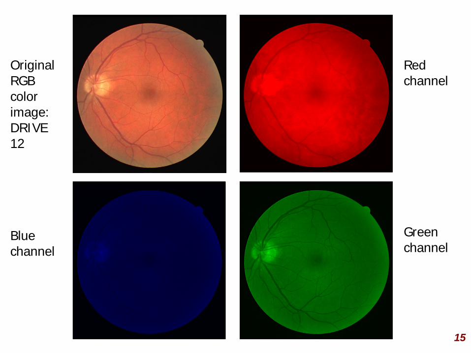
Original RGB color image: DRIVE 12
Blue channel
Red channel
Green channel
15
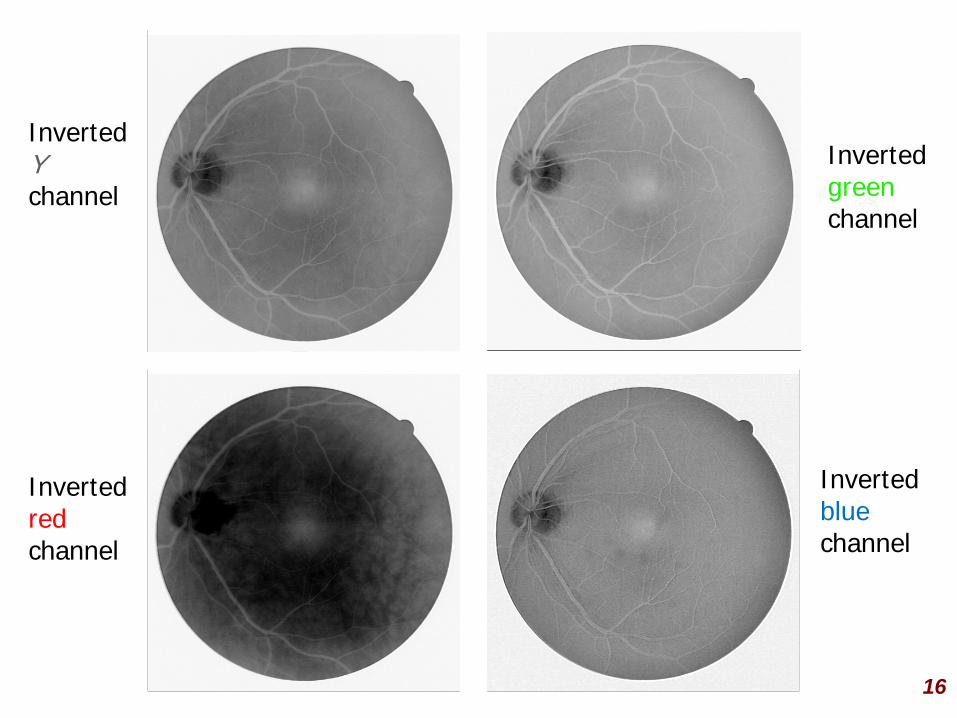
Inverted Y channel
Inverted green channel
Inverted red channel
Inverted blue channel
16
Selection of Color Image Components or Channels
The red & blue channels are noisy and are not suitable for the detection of blood vessels on their own.
The inverted green channel has the highest contrast among the RGB channels.
The blue and red channels contain useful information: higher contrast of vessels in the inverted Y channel.
17
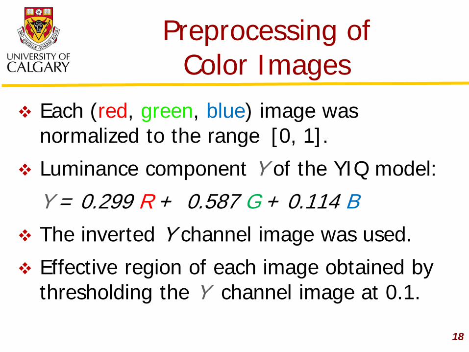
Preprocessing of Color Images
Each (red, green, blue) image was normalized to the range [0, 1].
Luminance component Y of the YIQ model:
Y = 0.299 R + 0.587 G + 0.114 B
The inverted Y channel image was used.
Effective region of each image obtained by thresholding the Y channel image at 0.1.
18

Preprocessing of Color Images
Morphological erosion applied with a disc-shaped structuring element of diameter 10 pixels to remove edge artifacts.
Pixels at the outer edge of the effective region identified using a four-pixel neighborhood.
Each pixel replaced by the mean over a 21 X 21 neighborhood within the effective
region.
19

Preprocessed Images
Y component extended Inverted Y component beyond the effective area 20

Gabor Filtering
Gabor filters were applied to the inverted and preprocessed Y channel.
A bank of 180 Gabor wavelets was used over the range of [-90o , 90o].
Parameters τ and l were varied over a large range to facilitate multiscale analysis and detection of curvilinear structures.
21

Results of Gabor Filtering
22
Log magnitude spectrum Inverted Y channel Magnitude response of a single Gabor wavelet: τ = 8, l = 2.9, θ = 45ο

τ = 2 l = 2.9 θ = 45ο
τ = 8 l = 6 θ = 45ο
τ = 2 l = 6 θ = 45ο
τ = 8 l = 2.9 θ = −45ο
23

Results of Gabor Filtering
Original Image Gabor Magnitude Gabor Angle (584 ×565) (max over 180 angles)
24

Original DRIVE 01
Blue: false positive Red: false negative
Result of detect- ion
Manual labeling
25

Results: ROC Az for 20
Images using the Y Channel
ROC : Receiver Operating Characteristics Az : Area under the ROC curve
26

Results: ROC Curve for the DRIVE Test Set
τ = 8, l = 2.9, Az = 0.94 27
Multifeature Analysis
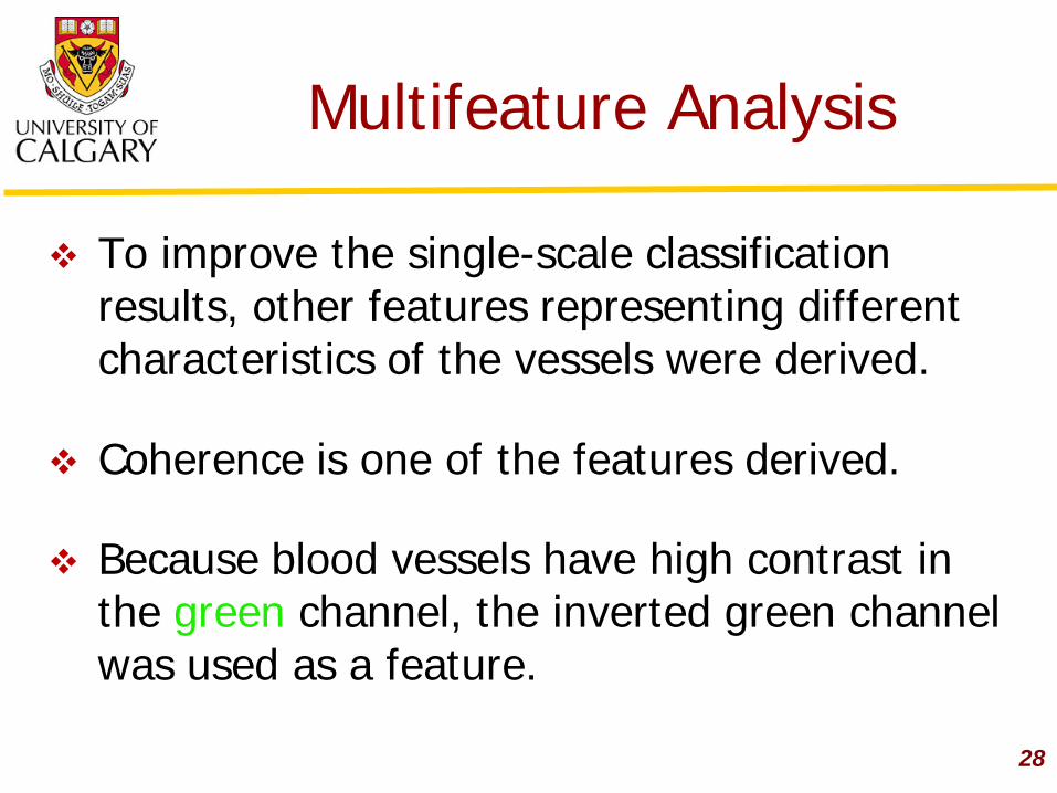
To improve the single-scale classification results, other features representing different characteristics of the vessels were derived.
Coherence is one of the features derived.
Because blood vessels have high contrast in the green channel, the inverted green channel was used as a feature.
28

Coherence
mnG
mnθ
pqψ
Coherence is a measure of the strength of orientation or anisotropy.
∑∑
∑∑
= =
= =
−= P
m
P
nmn
P
m
P
npqmnmn
pqpq
G
GG
1 1
1 1)cos( ψθ
γ
2)2cos(
)2sin(arctan
21
1 1
2
1 1
2
π
θ
θψ +=
∑∑
∑∑
= =
= =P
m
P
nmnmn
P
m
P
nmnmn
pq
G
G
: gradient magnitude, : gradient orientation, : local orientation.
29

30
Original Image
Gabor magnitude
Coherence Inverted green channel

Multifeature Analysis and Classification
Training and testing of the three features (Gabor magnitude, coherence, green channel) was done using various classifiers:
• Single-layer Perceptron (SLP): single-layer feed-forward (SLFF) artificial neural network (ANN). • Multilayered Perceptron (MLP). • Radial Basis Functions (RBF).
31

Results of Multifeature Analysis
Classification Method Az
Coherence only 0.8215 SLP (Gabor Magnitude and Coherence) with 10 nodes using 50% of the training data 0.9508 MLP (Gabor Magnitude and Coherence) with 2 layers (3 nodes and 1 node) using 50% of the training data 0.9507 MLP (Gabor Magnitude and Green) with 2 layers (3 nodes and 1 node) using 50% of the training data 0.9456 RBF (Gabor Magnitude and Coherence) with sigma=1.2 using 0.125% of the training data 0.9516
32
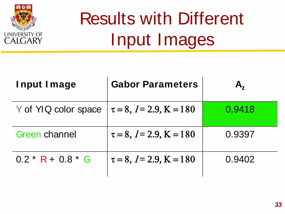
Results with Different Input Images
Input Image Gabor Parameters Az
Y of YIQ color space τ = 8, l = 2.9, Κ = 180 0.9418
Green channel τ = 8, l = 2.9, Κ = 180 0.9397
0.2 * R + 0.8 * G τ = 8, l = 2.9, Κ = 180 0.9402
33

Multiscale Gabor Filtering
Vessels in the retina vary in thickness: 50 to 200 μm.
The parameters of the Gabor filter ( τ , l ) may be varied to detect vessels at different scales of thickness and elongation.
Various combinations of scales were used for multiscale analysis.
34

Multiscale Analysis
1. Maximum Gabor response over all scales
2. Classifiers: I. Generic Multilayer Perceptron: 2 or 3 layers Using the discriminant function (tan-sig) Using 10% of training data
II. Radial Basis Functions: 8 or 15 nodes Sigma fixed at 1.2 Used 0.125% of training data
35

Results of Multiscale Analysis
Classifier # Layers # Nodes per layer
Scales Az
MLP 2 20, 1 τ = 8, 12 0.9522
MLP 2 20, 1 τ = 1, 4, 8 0.9554
MLP 2 20, 1 τ = 4, 8, 12 0.9592
MLP 3 20, 20, 1 τ = 0.5, 4, 8, 12 0.9587
MLP 3 30, 30, 1 τ = 4, 8, 12 0.9596
Classifier # Nodes Scales Az
RBF 8 τ = 4, 8, 12 0.9572
RBF 15 τ = 4, 8, 12 0.9565
RBF 8 τ = 0.5, 4, 8, 12 0.9565
RBF 8 τ = 1, 4, 8, 12 0.9547 36

Comparative Analysis with Other Works
37
Az values with 20 test images from DRIVE
Comparative Analysis
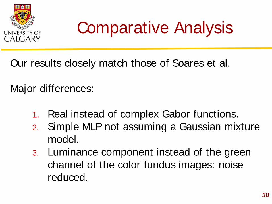
Our results closely match those of Soares et al. Major differences:
1. Real instead of complex Gabor functions. 2. Simple MLP not assuming a Gaussian mixture
model. 3. Luminance component instead of the green
channel of the color fundus images: noise reduced.
38

Remarks
Multiscale Gabor wavelets provide high efficiency in the detection of retinal blood vessels.
The proposed methods could assist in the diagnosis of various pathologies and localization of features.
Methods need to be developed to address the large number of false-positive pixels around the ONH.
Methods need be developed for optimal use of the information in the various color components.
39

Detection of the Optic Nerve Head in
Fundus Images of the Retina Xiaolu Iris Zhu, Rangaraj M. Rangayyan,
Fábio J. Ayres, and Anna L. Ells
Department of Electrical and Computer Engineering, Schulich School of Engineering, University of Calgary Division of Ophthalmology, Alberta Children's Hospital
Calgary, Alberta, Canada

The Optic Nerve Head
Need for the detection of the ONH:
Important anatomical feature (landmark).
Computer-assisted diagnosis.
A step in the early detection of retinal pathology.
41
DRIVE image 01 (584×565 pixels)

Objectives
Locate the approximate boundary of the ONH based on its circularity.
Locate the center of the ONH as the point of
convergence of the main blood vessels.
42

Detection of the ONH using the Hough Transform
Detect edges
Sobel operators or Canny method
Detect circles
Hough transform for the detection of circles
Select circle
Use intensity criterion to select the best-fitting circle for the ONH
43

Detection of Edges
Sobel Operators:
Combined gradient magnitude:
|G(x,y)| = [ Gx2 (x,y) + Gy
2 (x,y) ] 1/2
Canny Method Apply a threshold to obtain an edge map.
−−−
101202101
−−−
121000121
44

Detection of Circles: The Hough Transform
The points lying on the circle
( x – a )2 + ( y – b )2 = c2
are represented by a single point in the 3D parameter space (a, b, c)
Hough space: accumulator A (a, b, c)
45

Procedure to Detect Circles
1. Obtain a binary edge map of the preprocessed Y channel image.
2. Set ranges for a and b.
3. Solve for the value of c that satisfies ( x – a )2 + ( y – b )2 = c2 .
4. Update the accumulator corresponding to (a, b, c).
5. Update values for a and b within the range of interest and go back to Step 3.
46

Set Up of the Hough Space
Average diameter of the ONH: 1.5 mm.
Radius of a circular approximation to the ONH: 600 to 1000 μm.
Spatial resolution of the DRIVE images: 20 μm per pixel.
Range for the radius c : 31 to 50 pixels.
Size of the Hough space: 584×565×20. 47

Detection of Circles
48
Original image
Edge map
Hough space c = 20
Hough space c = 50

Detection of Circles
49
Original image
Edge map
Hough space c = 20
Hough space c = 50

Detection of Circles
DRIVE image 01 584×565 pixels
Edge map using Sobel
operators
Hough space
c=37 pixels
50

Hough-space Planes
c=31 pixels c=37 pixels c=47 pixels
51

Detection of the ONH
Check each of the top 30 potential circles indicated by the local maxima (peaks) in the Hough transform to verify if it could represent the ONH using a fraction of the reference intensity:
90% of the maximum intensity of the Y channel for the given image (DRIVE and STARE databases).
52

Results
DRIVE image 01
Edge map using Sobel operators
Successfully detected
ONH
53

Measure of Performance: Overlap
54

Distance: between the detected center and the center marked by an ophthalmologist.
Overlap: ratio of the intersection of the detected circular region and the ONH delineated by the ophthalmologist to their union.
Results: 40 DRIVE Images
Method Distance mm (pixels) Overlap
mean std mean std
First peak in the Hough space
1.05 (52.5) 1.87 (93.5) 0.58 0.36
Peak selected using intensity condition
0.36 (18) 1.00 (50) 0.73 0.25
55

Results: 81 STARE Images
Method Distance (pixels) Overlap
Mean std mean std
First peak in the Hough space
150.5 140.5 0.21 0.27
Peak selected using intensity condition
132.5 159 0.32 0.30
56

ONH Missed: STARE im0036
57

Detection of the ONH as the Convergence of Blood Vessels
1. Extract the orientation field using Gabor filters.
2. Filter and down-sample the orientation field.
3. Analyze the orientation field using phase portraits.
4. Post-process the phase portrait maps.
5. Detect sites of convergence of blood vessels.
6. Select the point of convergence to represent the center of the ONH.
58

Extract the Orientation Field
Compute the texture orientation (angle) for each pixel with l = 2.9, τ = 8 pixels.
59
Gabor filtering (line detection)

60
Extracting the Orientation Field
( )yx,I( )yx,g2
( )yxK ,g
Original image
( )yx,g1
Gabor filter bank (K = 180)
( )
( )K
kyx
yxk kk
ππθ max
max
2,
|},{|maxarg
+−=
= I
Orientation field
Image resolution: 20 µm/pixel Filtering
( )yx,1I
( )yx,2I
( )yxK ,I

Filtering and Down-sampling the Orientation Field
( )yx,θ
Orientation field
( )[ ]yx,2sin θ
( )[ ]yx,2cos θ
Gaussian filtering
Gaussian filtering
( )( )
yxcyxs
,,arctan
21
( )yxs ,
( )yxc ,
( )yxf ,θ
Filtered orientation field
4↓Downsample ( )yxd ,θ
Downsampled orientation field
Image resolution: 20 µm/pixel
Filtering
Downsampling
Image resolution: 80 µm/pixel

Phase Portraits
=
=
ed
cbba
bA ,
62
( ) bA , +
=
=
yx
vv
yxy
xv
node saddle spiral
,

Phase portrait type
Eigenvalues of matrix A Streamlines Orientation
field
Node Real, same sign
Saddle Real, opposite sign
Spiral Complex conjugate
63

Model Error
( ) ( )∑∑∆=x y
yx,, 22 bAε
( ) ( ) ( )[ ]bA,,,sin, yxyxyx φθ −=∆
( )bA,, yxφ( )yx,θOrientation field Model-generated field
Local error measure
Sum of the squared error measure

Phase Portrait Analysis (step 1 of 3)
1. Fit phase portrait model to the analysis window
65
−−
=
−
=
9.78.4
7.12.03.01.1
b
A
Window size: 40 × 40 pixels

Phase Portrait Analysis (step 2 of 3)
2. Find optimal phase portrait type and location of fixed point
bA 1−−=
=
yx
X
66
Type: node Fixed point: x=3, y=5
−−
=
−
=
9.78.4
7.12.03.01.1
b
A

Phase Portrait Analysis (step 3 of 3)
3. Cast a vote in the corresponding phase portrait map
67
Log (1+Node) [0, 1.526]
Orientation field
Log (1+Saddle) [0, 1.576]

Detection of the Center of the ONH
Check each peak in the node map to verify if it could represent the center of the ONH using a fraction of the reference intensity.
Fraction = 68% for the DRIVE images. Fraction = 50% for the STARE images.
68
69
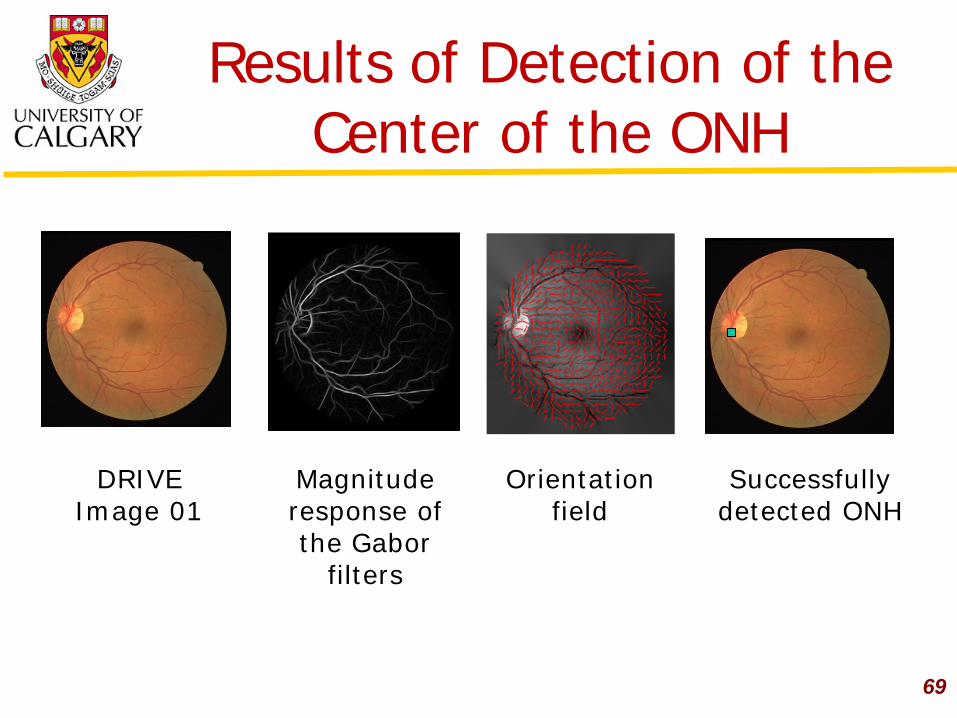
Results of Detection of the Center of the ONH
DRIVE Image 01
Magnitude response of the Gabor
filters
Orientation field
Successfully detected ONH

Successful Detection with Difficult Images
70 DRIVE 34 STARE im0021

71
STARE image im0139 (700×605 pixels),
distance = 321 pixels
Image im0010, distance = 2.2 pixels
Results of Detection of the Center of the ONH

Statistics for the 40 images in the DRIVE database.
72
Method Distance mm (pixels)
mean std First peak in node map 1.61 (80.7) 2.40 (120)
Peak selected using intensity condition
0.46 (23.2) 0.21 (10.4)
Results of Detection of the Center of the ONH
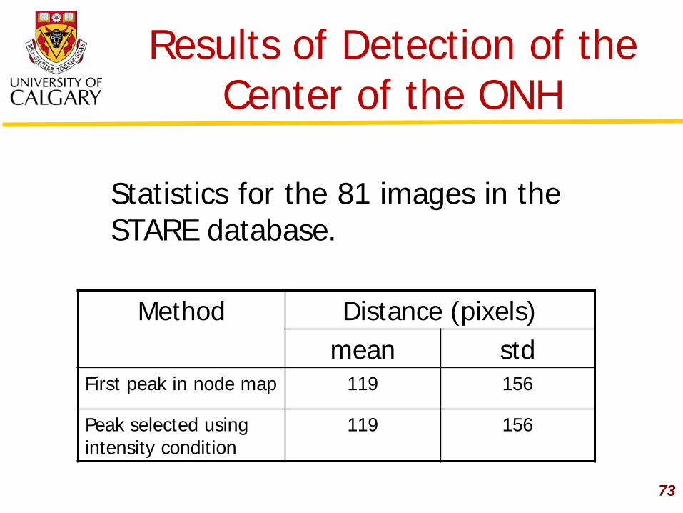
73
Statistics for the 81 images in the STARE database.
Method Distance (pixels) mean std
First peak in node map 119 156
Peak selected using intensity condition
119 156
Results of Detection of the Center of the ONH
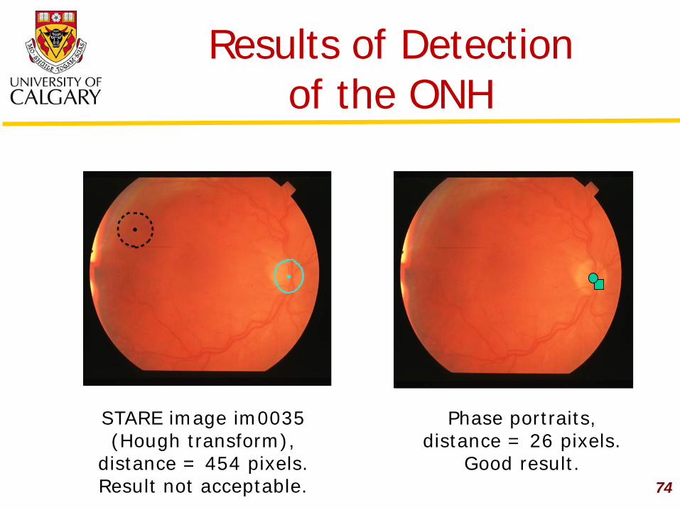
STARE image im0035 (Hough transform),
distance = 454 pixels. Result not acceptable.
Phase portraits, distance = 26 pixels.
Good result. 74
Results of Detection of the ONH

Free-response Receiver Operating Characteristics: 40 images of DRIVE
75

Free-response Receiver Operating Characteristics: 81 images of STARE
76
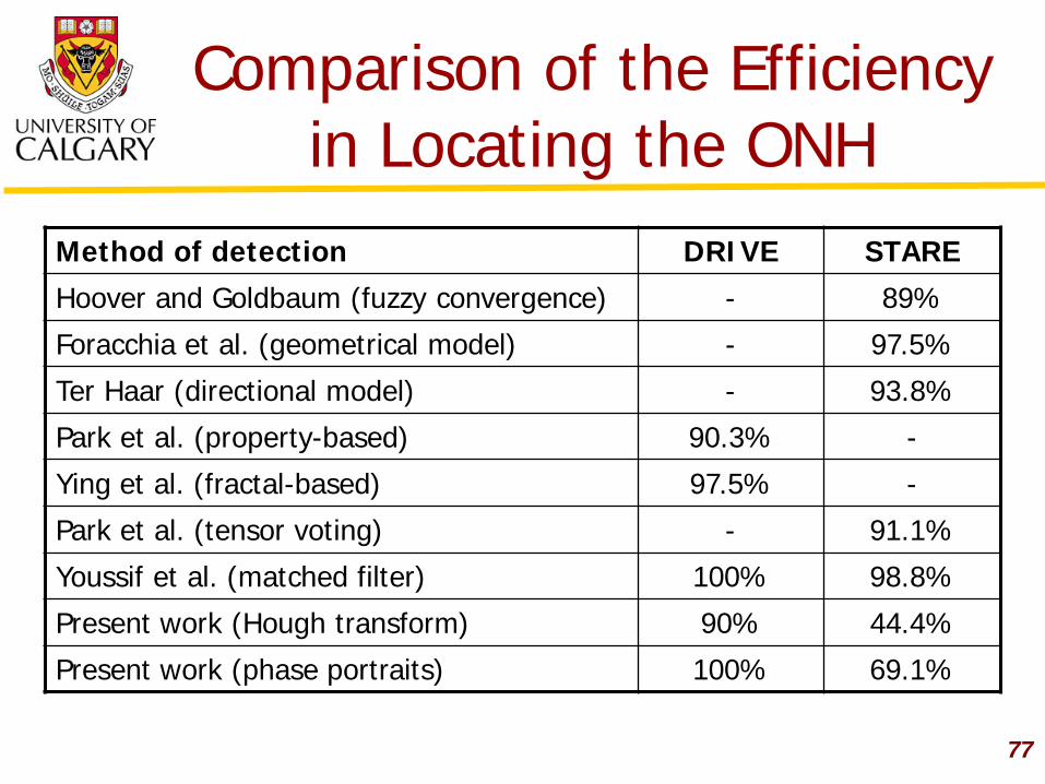
Comparison of the Efficiency in Locating the ONH
Method of detection DRIVE STARE
Hoover and Goldbaum (fuzzy convergence) - 89%
Foracchia et al. (geometrical model) - 97.5%
Ter Haar (directional model) - 93.8%
Park et al. (property-based) 90.3% -
Ying et al. (fractal-based) 97.5% -
Park et al. (tensor voting) - 91.1%
Youssif et al. (matched filter) 100% 98.8%
Present work (Hough transform) 90% 44.4%
Present work (phase portraits) 100% 69.1%
77
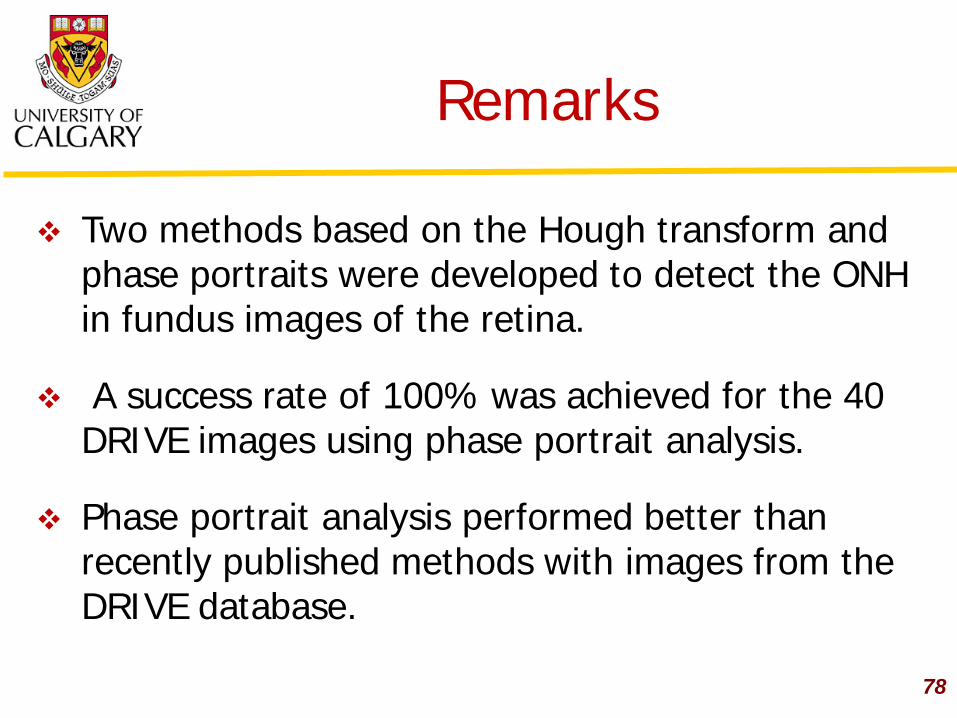
78
Two methods based on the Hough transform and phase portraits were developed to detect the ONH in fundus images of the retina.
A success rate of 100% was achieved for the 40 DRIVE images using phase portrait analysis.
Phase portrait analysis performed better than recently published methods with images from the DRIVE database.
Remarks

Modeling and Parametric Representation of the
Retinal Temporal Arcade
Faraz Oloumi, Rangaraj M. Rangayyan, Anna L. Ells
Department of Electrical and Computer Engineering Schulich School of Engineering, University of Calgary Division of Ophthalmology, Alberta Children's Hospital
Calgary, Alberta, Canada

Retinal Temporal Arcade in Fundus Images
80 ONH = Optic Nerve Head
Fovea
Superior Temporal Arcade
ONH
Inferior Temporal Arcade
Major Temporal Arcade

The vessels in the retina are modified in terms of their width, shape, and tortuosity.
ROP is the leading cause of preventable childhood blindness.
Plus disease is used as an indicator of the severity of ROP.
Retinopathy of Prematurity (ROP)
81

Plus disease has been difficult to define in a quantitative manner.
Diagnosis is made by visual, qualitative comparison.
Abnormal dilation, tortuosity, and a decrease in the angle of insertion of the major temporal arcade (MTA) are symptoms of plus disease.
Plus Disease
82

Gold-standard Images
Two gold-standard images used as references for the diagnosis of dilation and tortuosity due to
plus disease. 83

In a study to measure the level of agreement between experts there was:
27% disagreement (18 of 67) on the presence of plus disease.
37% and 31% disagreement on the presence of tortuosity and dilation due to plus disease.
Computer algorithms needed for automated detection and analysis of retinal vessels.
Limitations of Visual Comparative Analysis
84
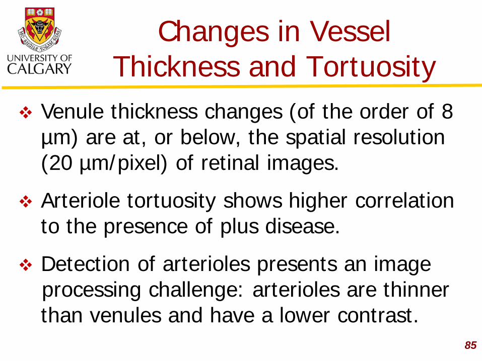
Venule thickness changes (of the order of 8 µm) are at, or below, the spatial resolution (20 µm/pixel) of retinal images.
Arteriole tortuosity shows higher correlation to the presence of plus disease.
Detection of arterioles presents an image processing challenge: arterioles are thinner than venules and have a lower contrast.
Changes in Vessel Thickness and Tortuosity
85

There are inherent limitations in using vessel thickness and tortuosity as indicators.
The angle of insertion of the MTA is an indicator of posterior structural integrity.
A decrease in this angle can be a sequela of ROP.
The temporal arcade angle (TAA) is defined by Wilson et al. as:
TAA = superior arcade angle (SAA) + inferior arcade angle (IAA).
Angle of Insertion of the MTA
86

Angle of Insertion of the MTA
Fovea (F) and ONH (O) are manually marked. The image is rotated so
that the line OF (retinal raphe) is horizontal.
The normal (AB) to OF is drawn at F up to the MTA.
TAA = IAA + SAA SAA= tan-1(FB/OF) IAA= tan-1(FA/OF) .
87
F
B
A
O IAA
SAA

There is a high degree of symmetry between the angle of insertion of the two eyes of an individual.
Asymmetry above 14º to 20º is suspicious.
A significant level of vessel angle acuteness is associated between stages 0 and 1, stages 1 and 2, and stages 1 and 3 of ROP in the IAA of the left eye.
Changes in the Angle of Insertion
88

The MTA has not been modeled for quantitative
analysis of its openness.
The parabolic profile of the MTA could allow for effective modeling using the generalized Hough transform (GHT).
Changes in the TAA are expected to be reflected as changes in the openness parameter of a parabolic model.
Detection of the MTA
89

Two steps in modeling the MTA:
1. Derivation of a vessel map: magnitude output of the Gabor filter bank.
2. Detection of parabolas: the generalized Hough transform.
Parametric Modeling of the MTA
90

Derivation of the Vessel Map
The magnitude output of the Gabor filters can be used for this purpose.
A large value for thickness (τ = 16) is used to emphasize the MTA with l = 2.
The Gabor magnitude image is binarized using a fixed threshold.
The binary image is skeletonized. The skeleton image is cleaned using the
morphological area open procedure. 91

Original
Skeleton
Vessel Map
Cleaned Skeleton
92

The GHT for Parabolic Modeling
The GHT is a flexible method for parameterizing curves such as parabolas.
The general formula defining a parabola:
where is the vertex, and is the openness parameter.
)(4)( 2oo xxayy −=−
),( oo yxa
93

A Parabolic Model
The value of defines the the openness or aperture of the parabola and the direction it opens to; for a positive value the parabola opens to the right and vice versa. In this 584 × 565 image,
a = +59.
a
a
94

The GHT for Parabolic Modeling
The parameters define the Hough space, represented by an accumulator A.
For every non-zero pixel in the image domain, there exists a parabola in the Hough space for each value of .
A single point in the Hough space defines a parabola in the image domain.
),,( ayx oo
a
95

Detection of the Parabolas
For every non-zero pixel in the image the parameter a is computed for each in the Hough space and the accumulator is incremented. The point with the highest value represents the best fitting parabola.
),( oo yx
96 Hough space
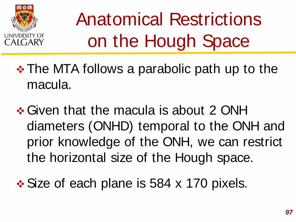
Anatomical Restrictions on the Hough Space
The MTA follows a parabolic path up to the macula.
Given that the macula is about 2 ONH diameters (ONHD) temporal to the ONH and prior knowledge of the ONH, we can restrict the horizontal size of the Hough space.
Size of each plane is 584 x 170 pixels.
97

Anatomical Restrictions on the Hough Space
The location of the vertex of the desired parabola in the Hough space is restricted to be within 0.25 * ONHD of the ONH.
The value of has a physiological limit: set to be within the range [35, 120] for DRIVE images.
The number of planes in the 3D Hough space is 86.
a
98

*Hough space updated with Gabor Mag. with vertex and horizontal size restrictions.*
Hough space updated with unity.
Hough space updated with unity with vertex and horizontal size restrictions.
Hough space updated with Gabor Mag. with horizontal size restriction.
99

Parabolic Fits to the MTA
Global max. in the Hough space: Gabor-magnitude-updated: a = -65. Gabor-magnitude-updated with vertex restriction: a = -75. Unity-updated with vertex restriction: a = -66.
100

Correction of the Retinal Raphe Angle
The line going through the fovea and the center of the ONH is the retinal raphe.
Any rotation that might exist between the retinal raphe and the horizontal axis of the image should be corrected.
101

The rotation angle was found automatically by using the manual markings of the ONH and the fovea.
The original image was rotated by the determined angle by using bilinear interpolation and cropping the image to its original size.
102
Correction of the Retinal Raphe Angle

MDCP Measure
The MDCP measures the closeness of two given contours based on the mean of the distance to the
closest point (DCP) from one of the contours (the model) to the other (the reference).
Given a model, M = {m1,m2, ..., mN}, and a reference R = {r1, r2, ..., rK}, the DCP for a single point on M is defined as:
where is a norm operator. 103
( ) KjrmRm jii ,...,2,1, min),(DCP =−=

MDCP Measure
The MDCP is computed as
The top 10 Hough-space candidates were selected for MDCP analysis.
104
∑=
=N
ii Rm
NRM
1),(DCP1),(MDCP

Choosing Between the Top Hough-space Candidates
By taking the parabolic fits to be the model (M) and the automatically obtained skeleton to be the reference (R), the MDCP was calculated for each of the top 10 candidates.
The parabola with the lowest MDCP value was selected as the best fit to the MTA.
105

Dual-parabolic Modeling
The ITA and the STA are often asymmetric; a single parabolic model may match either one of the arcades, but not both.
Modeling each part of the arcade separately may be a more suitable option.
To represent the ITA, any information above the detected center of the ONH was eliminated in the Gabor magnitude response image.
106

Dual-parabolic Modeling
The STA was represented by excluding the information in the Gabor magnitude response image below the detected center of the ONH.
The upper part of the parabolic fit to the STA was taken as the STA model.
The lower part of the parabolic fit to the ITA was taken as the ITA model.
107

Dual-parabolic Modeling
108 Parabolic fit using Gabor- Dual-parabolic fit using magnitude-updated GHT Gabor-magnitude-updated GHT

Performance Measures
The MTAs for all 40 DRIVE images were drawn by an expert ophthalmologist.
Two types of performance measure: 1. The accuracy of the parabolic model fitted to the
vessel skeleton (Auto) as compared to the parabolic model fitted to the hand-drawn contour (Hand).
2. The accuracy of the parabolic model fitted to the vessel skeleton as compared to the hand-drawn contour.
109

The fits to the hand-drawn traces were obtained using all versions of the Hough space.
A distance error measure was obtained in terms of the Euclidean distance between the two detected vertices as:
The correlation coefficient between the two sets of
values was also computed: where is the
covariance.
Comparing the Parabolic Models
22 )()(AutoHandAutoHand oooo yyxx −+−
),(),(),(
HandHandAutoAuto
AutoHand
aaCaaCaaC
a
C110

The automatic fit (solid green) Both fits are accurate. is matching the arteriole. Cyan: fit to hand-drawn MTA.
111
Results of Parabolic Modeling

Accuracy of the Parabolic Model
To assess the accuracy of the obtained parabolic fits compared to the hand-drawn MTA, the MDCP was used as a distance error measure.
Parabolic fits were obtained using the four versions of GHT as described before with the added options of MDCP-based selection and correction of the raphe angle.
112

113
MDCP= 17.63 pixels
With raphe angle correction MDCP = 12.63 pixels
With vertex restriction MDCP = 25.04 pixels
With MDCP-based selection MDCP = 12.33 pixels.

Results: Dual-parabolic Modeling
Single model: MDCP = 11.5 Dual model: MDCP = 3.11 114
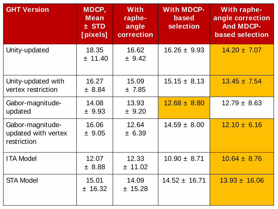
GHT Version MDCP, Mean ± STD
[pixels]
With raphe-angle
correction
With MDCP-based
selection
With raphe-angle correction
And MDCP-based selection
Unity-updated 18.35 ± 11.40
16.62 ± 9.42
16.26 ± 9.93 14.20 ± 7.07
Unity-updated with vertex restriction
16.27 ± 8.84
15.09 ± 7.85
15.15 ± 8.13 13.45 ± 7.54
Gabor-magnitude-updated
14.08 ± 9.93
13.93 ± 9.20
12.68 ± 8.80 12.79 ± 8.63
Gabor-magnitude-updated with vertex restriction
16.06 ± 9.05
12.64 ± 6.39
14.59 ± 8.00 12.10 ± 6.16
ITA Model 12.07 ± 8.88
12.33 ± 11.02
10.90 ± 8.71 10.64 ± 8.76
STA Model 15.01 ± 16.32
14.09 ± 15.28
14.52 ± 16.71 13.93 ± 16.06

Parabolic modeling could assist in quantitative analysis of changes in retinal vasculature.
Two factors causing inaccuracy in the models:
1. Distinct presence of arterioles and other vessels: a procedure to detect and eliminate arterioles may be used.
2. High slope of arcades at the ONH: An exponential model fitted to each arcade separately may lead to better models.
Remarks
116

Graphical User Interface
117

Method of Wong et al.
Mark the center of the ONH.
Center image on the ONH.
Crop image to circle of diameter 240 pixels.
Manually mark the largest venule branches.
Vertex of the angle is the center of the ONH.
Two points marked at the intersection of a circle of radius 60 pixels with the venule branch to define the arcade angle.
118

119
Results: Application to PDR
Normal: aMTA = -153 aSTA = -138, aITA = -420 TAA = 157.8 o
PDA: aMTA = 55 aSTA = 36, aITA = 48 TAA = 110.4 o
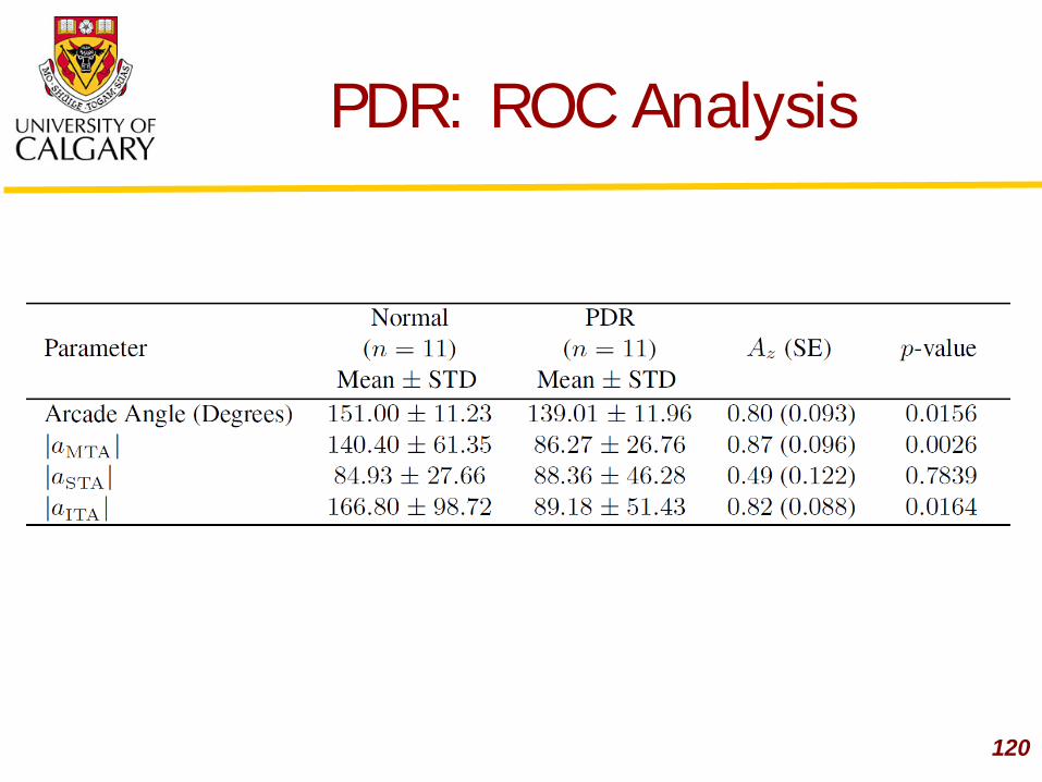
PDR: ROC Analysis
All Values are in degrees
120

121
Results: Application to RoP
RoP 0
RoP 2
RoP 1
RoP 3

122
Results: Application to RoP

RoP: ROC Analysis
All Values are in degrees
123
Remarks
The method of Wilson et al. is inapplicable to most cases of PDR used in this work.
The radius of the circle in the method of Wong et al. affects the arcade angle.
No other study has quantitatively measured the narrowing of the MTA due to PDR.
The parameters of the parabolic model could assist in diagnosis and follow up.
124

125
Thank You!
Natural Sciences and Engineering Research Council of Canada.
My students, coworkers, and collaborators.


![IEEE TRANSACTIONS ON PATTERN ANALYSIS AND …ds/Papers/BoCS08.pdfpattern used to probe the input image. ... was proposed by Gordon and Rangayyan [20] ... topological properties of](https://img.pdfslide.us/doc/110x75/5aa8cfe07f8b9a8b188c0588/ieee-transactions-on-pattern-analysis-and-dspapers-used-to-probe-the-input.jpg)


![IJECT V . 7, I 1, J - M 2016 Proposed Algorithm for ... · [1] “Lesson 17: Heart Sound”, Biopac Student Lab 3.7.6. [2] Lehner RJ, Rangayyan RM.,“A three-channel microcomputer](https://img.pdfslide.us/doc/110x75/5e30b9f46b4afa240e4cbe39/iject-v-7-i-1-j-m-2016-proposed-algorithm-for-1-aoelesson-17-heart.jpg)