Biomedical SignalsSignals and Images in Medicine

Lecture 4

Dr Nabeel Anwar

Before we start…

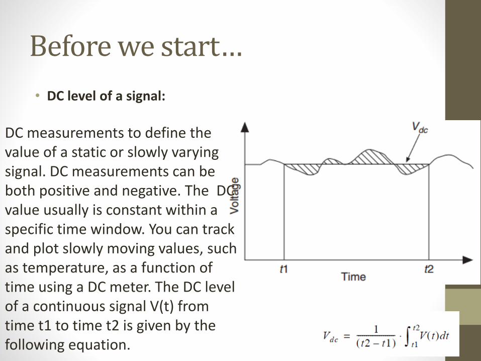
• DC level of a signal:

DC measurements to define the value of a static or slowly varying signal. DC measurements can be both positive and negative. The DC value usually is constant within a specific time window. You can track and plot slowly moving values, such as temperature, as a function of time using a DC meter. The DC level of a continuous signal V(t) from time t1 to time t2 is given by the following equation.

Before we start…

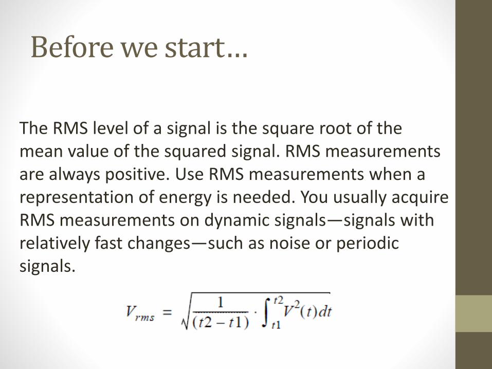
The RMS level of a signal is the square root of the mean value of the squared signal. RMS measurements are always positive. Use RMS measurements when a representation of energy is needed. You usually acquire RMS measurements on dynamic signals—signals with relatively fast changes—such as noise or periodic signals.

Problem

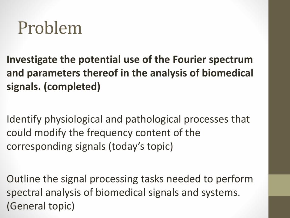
Investigate the potential use of the Fourier spectrum and parameters thereof in the analysis of biomedical signals. (completed)

Identify physiological and pathological processes that could modify the frequency content of the corresponding signals (today’s topic)

Outline the signal processing tasks needed to perform spectral analysis of biomedical signals and systems. (General topic)

5

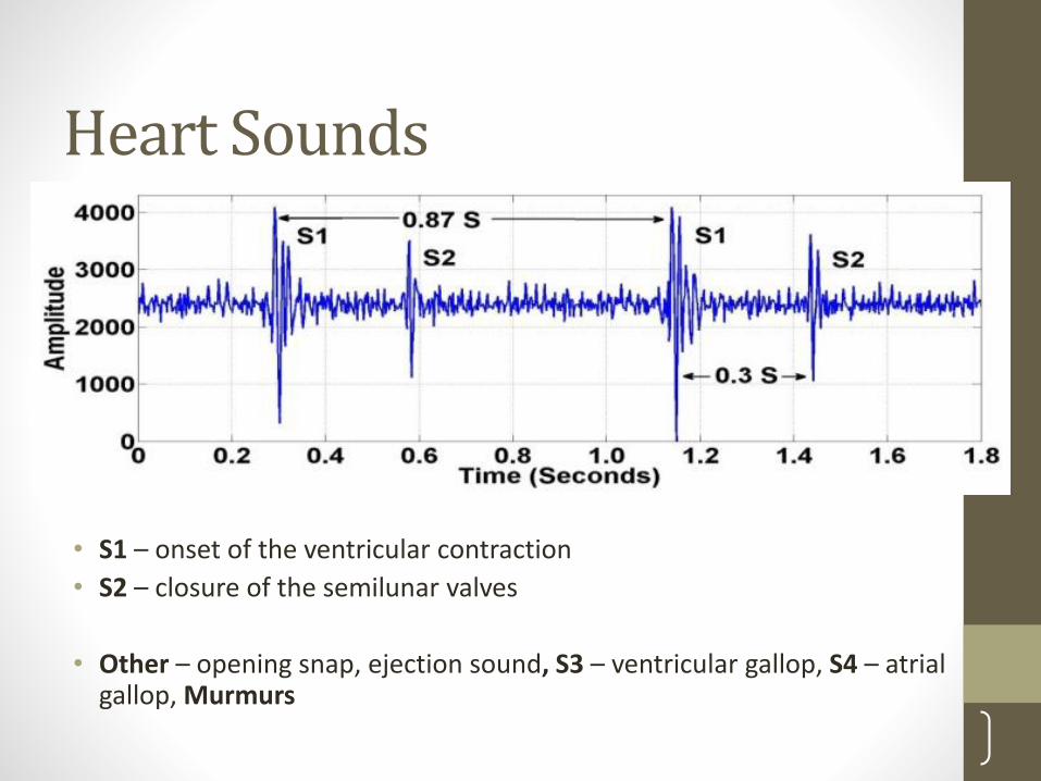
Heart Sounds

• S1 – onset of the ventricular contraction

• S2 – closure of the semilunar valves

• Other – opening snap, ejection sound, S3 – ventricular gallop, S4 – atrial gallop, Murmurs

6

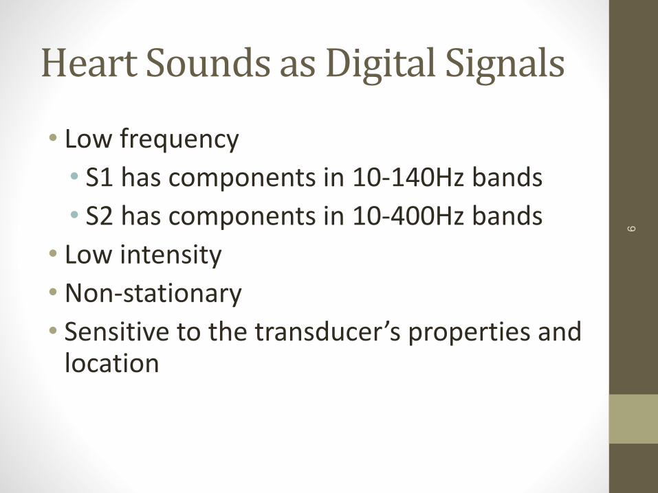
Heart Sounds as Digital Signals

• Low frequency

• S1 has components in 10-140Hz bands

• S2 has components in 10-400Hz bands

• Low intensity

• Non-stationary

• Sensitive to the transducer’s properties and location

Rangaraj Book Self Reading Chapter 6

Case Study: The effect of myocardial elasticity on heart sound spectra

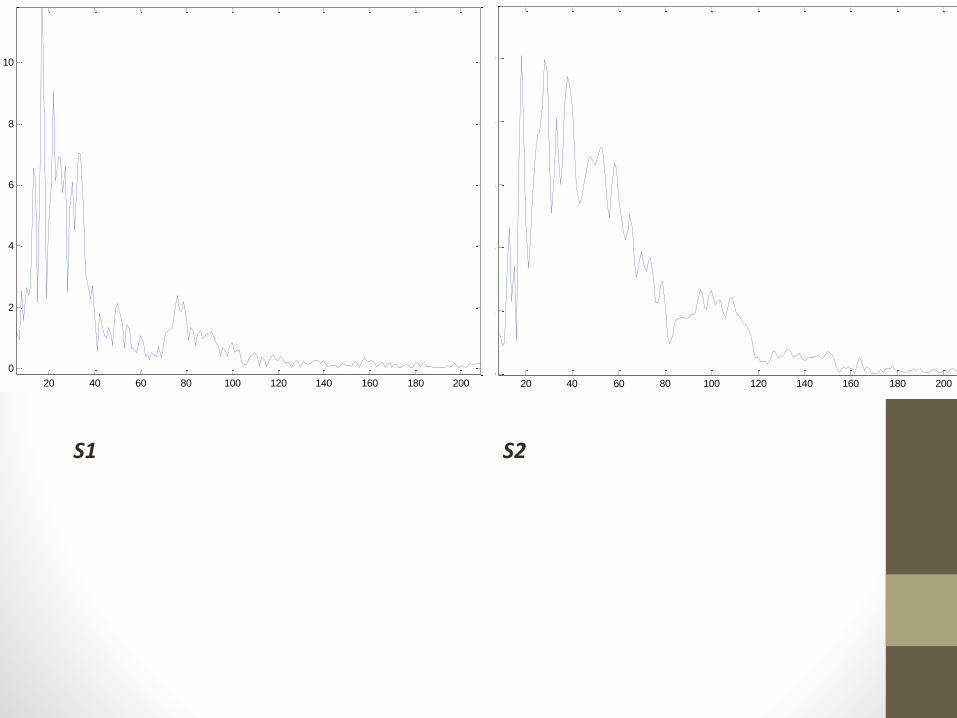
The first and second heart sounds — S1 and S2 —are typically composed of low-frequency components, due to the fluid-filled and elastic nature of the cardiohemic system.

20 40 60 80 100 120 140 160 180 2000

2

4

6

8

10

20 40 60 80 100 120 140 160 180 200

0

2

4

6

8

10

S1 S2

Problem statement

Constrained flow of blood through an orifice (septal defect) or across a stenosed valve acting leads to turbulence: wide-band noise.

So we need to consider the distribution of the signal’s energy or power over a wide band of frequencies: leads to the notion of the power spectral density function.

PSD is a measure of how power in a signal changes as a function of frequency.

Case study: Frequency analysis to diagnose valvular defects

1. Cardiovascular valvular defects and diseases cause

high-frequency, noise-like sounds known as murmurs.

Murmur of mitral stenosis: limited to less than 400 Hz.

Aortic insufficiency combined with mitral stenosis: more high-frequency energy in the range 300 − 1, 000 Hz.

2. Trans-aortic-valvular systolic pressure gradient measured

with catheterization and cardiac fluoroscopy: 10 − 140 mm of Hg.

Spectral power ratios computed with the bands

25 − 75 Hz : constant area (CA) related to normal sounds,

75 − 150 Hz : predictive area (P A) related to murmurs.

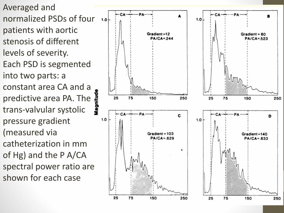
Averaged and normalized PSDs of four patients with aortic stenosis of different levels of severity.Each PSD is segmented into two parts: a constant area CA and a predictive area PA. The trans-valvular systolicpressure gradient (measured via catheterization in mm of Hg) and the P A/CA spectral power ratio are shown for each case

• The last slide gives an idea about spectral distribution over the range of frequencies, we name it Power spectral density (PSD).

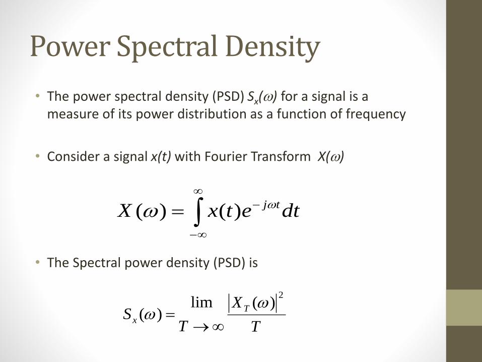
Power Spectral Density

• The power spectral density (PSD) Sx(w) for a signal is a measure of its power distribution as a function of frequency

• Consider a signal x(t) with Fourier Transform X(w)

• The Spectral power density (PSD) is

T

X

TS

T

x

2)(lim

)(w

w

dtetxX tjww )()(

PSD in Phonocardiogram (PCG)Interesting examples of a signal with multiple frequency-domain features.

• Beat-to-beat periodicity or rhythm.

• Heart sounds within a cardiac cycle exhibit resonance.

• Multi-compartmental nature of the cardiac system:

• multiple resonance frequencies: composite spectrum of several dominant or resonance frequencies.

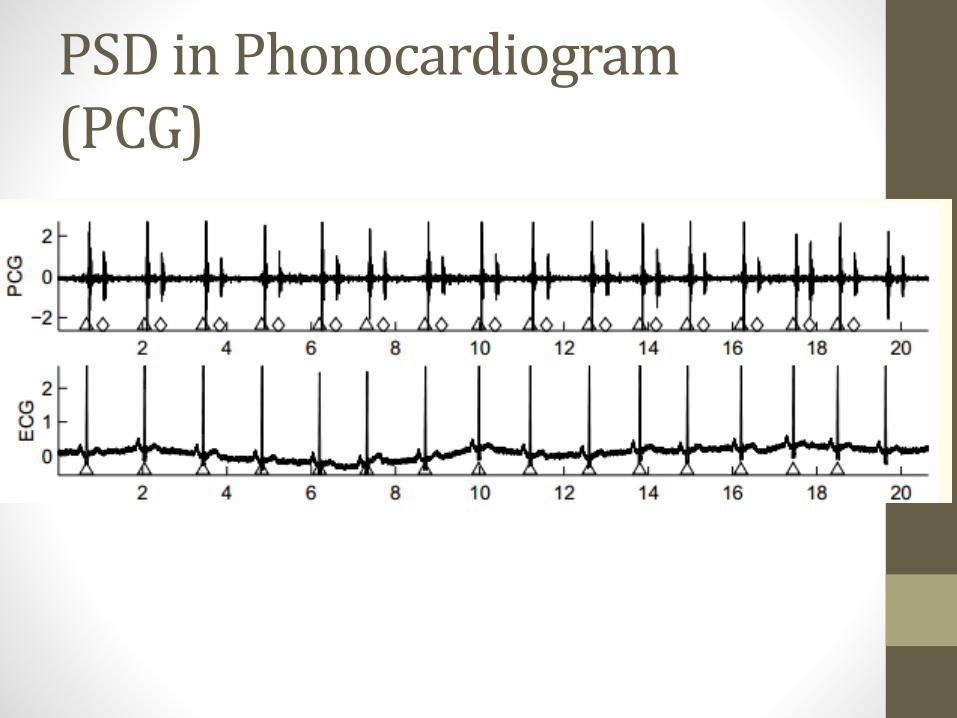
PSD in Phonocardiogram (PCG)

PSD in Phonocardiogram (PCG)With phonocardiogram we can detect S1 and S2 (first and second heart sound).

Heart sound spectra

S1: peaks at lower frequencies than those of S2;

S2: “gentle peaking” between 60 Hz and 220 Hz.

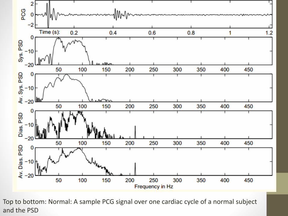
Top to bottom: Normal: A sample PCG signal over one cardiac cycle of a normal subject and the PSD

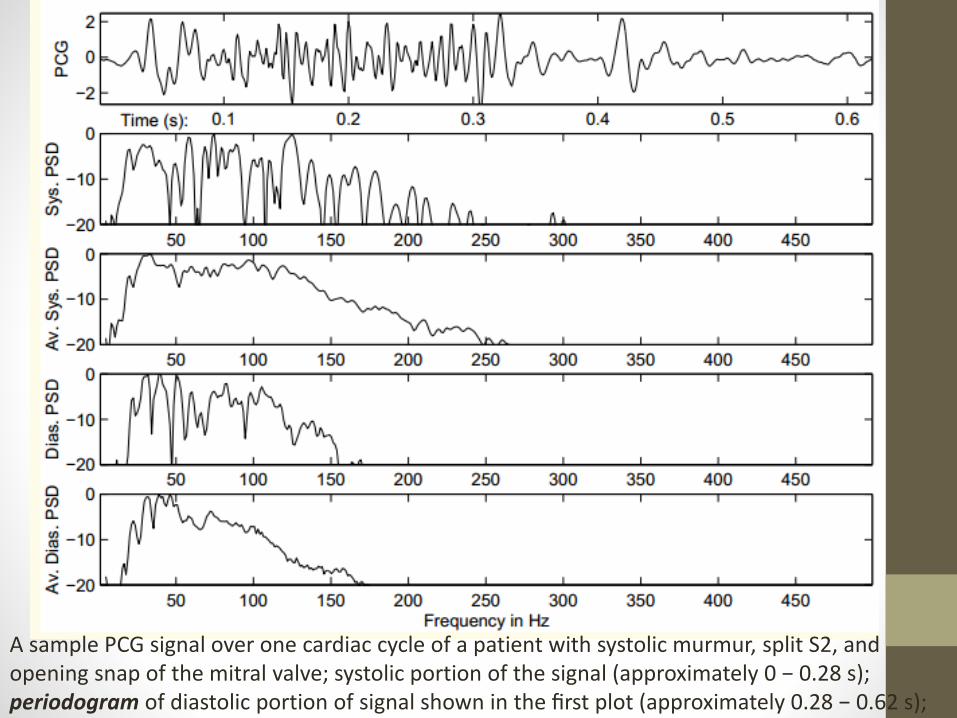
A sample PCG signal over one cardiac cycle of a patient with systolic murmur, split S2, and opening snap of the mitral valve; systolic portion of the signal (approximately 0 − 0.28 s); periodogram of diastolic portion of signal shown in the first plot (approximately 0.28 − 0.62 s);

Periodogram

A periodogram is a method of calculating the power spectral density (PSD) of a signal. A simple periodogram involves dividing the data into windows and computing the PSD of each window, then taking the mean of these individual PSDs.

Periodogram is the spectrum of a set of time signal usually obtained by fast Fourier transform (FFT). It usually shows frequency as x-axis, and magnitude of spectrum as y-axis.

Periodogram Approach

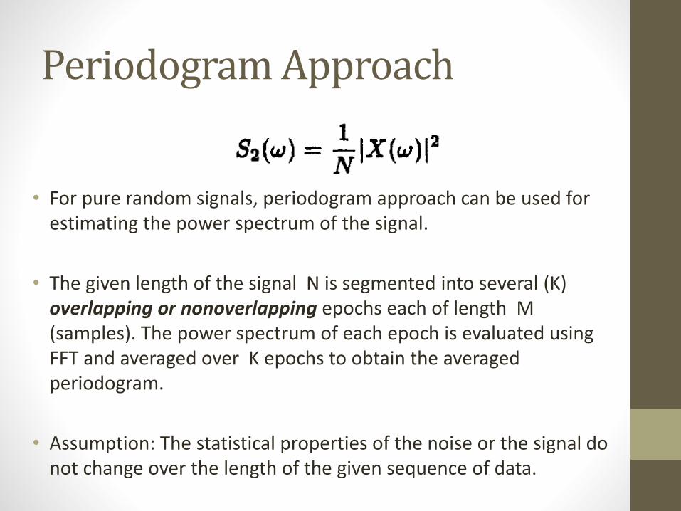
• For pure random signals, periodogram approach can be used for estimating the power spectrum of the signal.

• The given length of the signal N is segmented into several (K) overlapping or nonoverlapping epochs each of length M(samples). The power spectrum of each epoch is evaluated using FFT and averaged over K epochs to obtain the averaged periodogram.

• Assumption: The statistical properties of the noise or the signal do not change over the length of the given sequence of data.

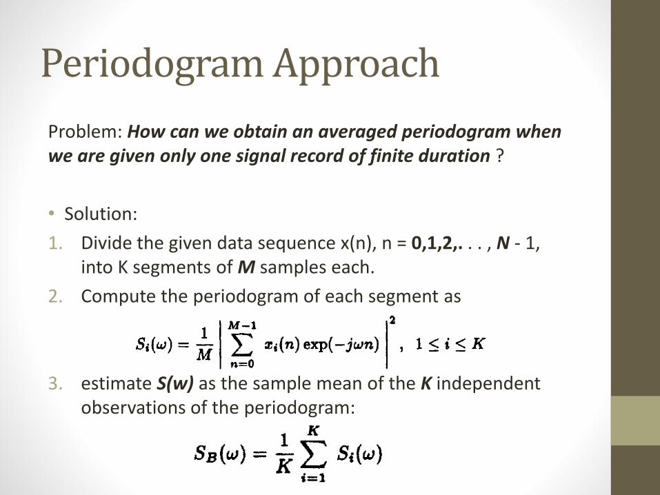
Problem: How can we obtain an averaged periodogram when we are given only one signal record of finite duration ?

• Solution:

1. Divide the given data sequence x(n), n = 0,1,2,. . . , N - 1, into K segments of M samples each.

2. Compute the periodogram of each segment as

3. estimate S(w) as the sample mean of the K independent observations of the periodogram:

Periodogram Approach

What is the benefit by having K epochs?

Variance Reduction: The variance (or uncertainty) in the individual estimates is inversely proportional to K. Therefore, it is desirable to increase the number of segments K in order to decrease the uncertainty in the estimates. Averaging all K makes the signal more reliable.

However; increasing K will also decrease the resolution in the power spectra (you already know why).

Ans: In non-overlapping case: If we increase the K, the number of samples M per segment will be reduced, small signal length means the main lobe of FFT widened, and frequency resolution lost.

Periodogram Approach

Periodogram Approach

We will consider two methods for periodogram

1. Bartlett periodogram; It is generated by dividing the data sequence of N points into K usually non-overlapping segments of M sample points each, N = KM.

• We have K number of epoches so We compute K number estimates of power spectra at each frequency and average the K values.

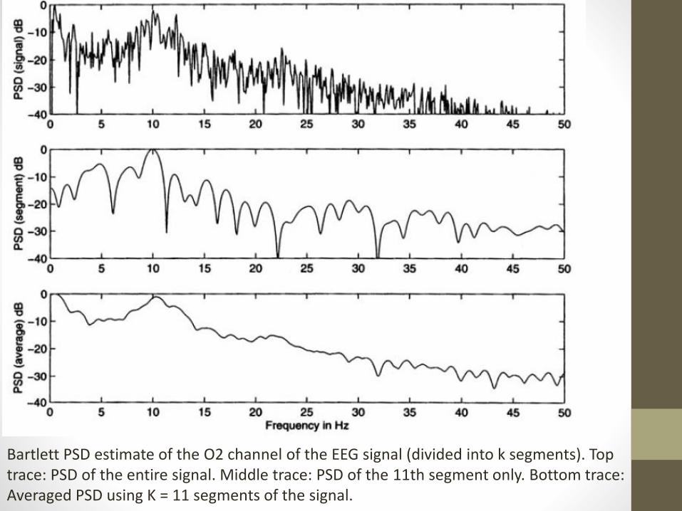
Bartlett PSD estimate of the O2 channel of the EEG signal (divided into k segments). Top trace: PSD of the entire signal. Middle trace: PSD of the 11th segment only. Bottom trace: Averaged PSD using K = 11 segments of the signal.

Periodogram Approach

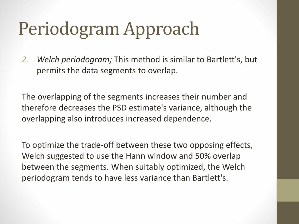
2. Welch periodogram; This method is similar to Bartlett's, but permits the data segments to overlap.

The overlapping of the segments increases their number and therefore decreases the PSD estimate's variance, although the overlapping also introduces increased dependence.

To optimize the trade-off between these two opposing effects, Welch suggested to use the Hann window and 50% overlap between the segments. When suitably optimized, the Welch periodogram tends to have less variance than Bartlett's.

• Both Bartlette and Welche are used for variance reduction in PSD.

Spectrogram

The main difference between spectrogram and periodogram is whether time locality is emphasized.

Periodogram is PSD and an average of K epochs, plotted on magnitude of spectrum - frequency graph.

A spectrogram is a multiple short periods of spectrum combined together. It is three dimensional by nature, that is time, frequency and magnitude of spectrum three dimensions.

Example: sleep spindles

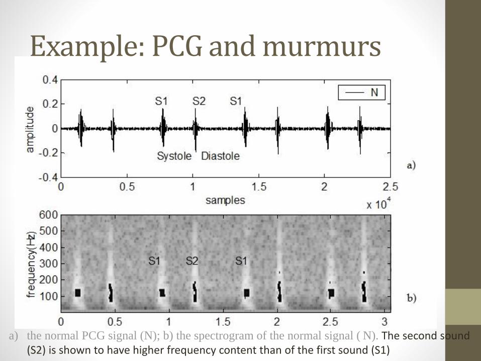
a) the normal PCG signal (N); b) the spectrogram of the normal signal ( N). The second sound (S2) is shown to have higher frequency content than of the first sound (S1)

Example: PCG and murmurs

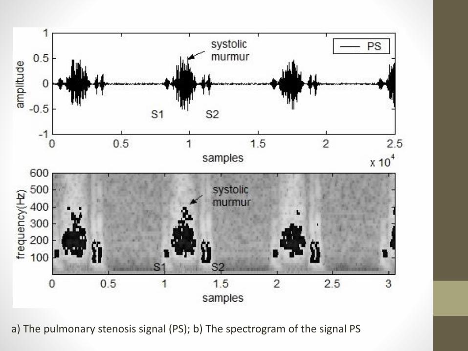
a) The pulmonary stenosis signal (PS); b) The spectrogram of the signal PS

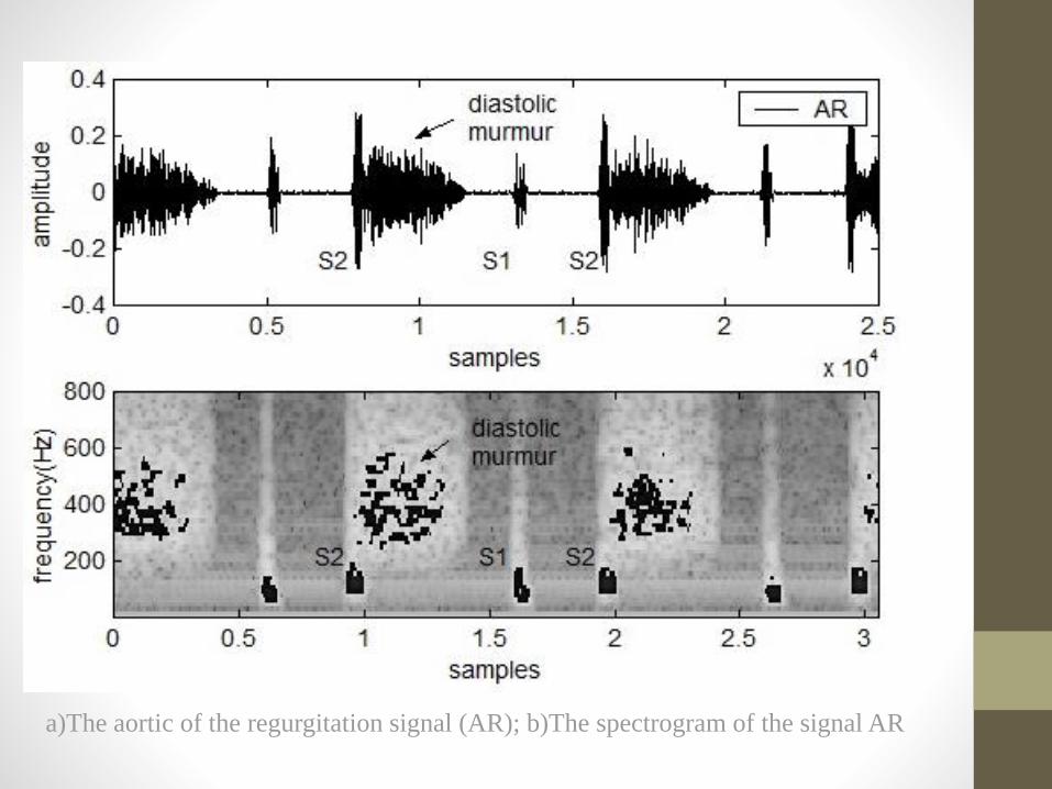
a)The aortic of the regurgitation signal (AR); b)The spectrogram of the signal AR

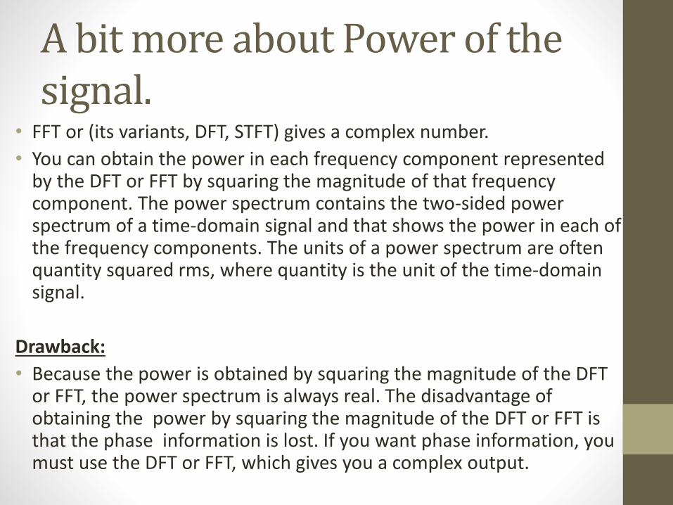
A bit more about Power of the signal.

• FFT or (its variants, DFT, STFT) gives a complex number.

• You can obtain the power in each frequency component represented by the DFT or FFT by squaring the magnitude of that frequency component. The power spectrum contains the two-sided power spectrum of a time-domain signal and that shows the power in each of the frequency components. The units of a power spectrum are often quantity squared rms, where quantity is the unit of the time-domain signal.

Drawback:

• Because the power is obtained by squaring the magnitude of the DFT or FFT, the power spectrum is always real. The disadvantage of obtaining the power by squaring the magnitude of the DFT or FFT is that the phase information is lost. If you want phase information, you must use the DFT or FFT, which gives you a complex output.

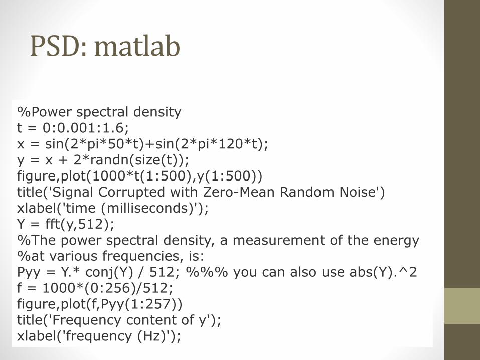
PSD: matlab

%Power spectral densityt = 0:0.001:1.6;x = sin(2*pi*50*t)+sin(2*pi*120*t);y = x + 2*randn(size(t));figure,plot(1000*t(1:500),y(1:500))title('Signal Corrupted with Zero-Mean Random Noise')xlabel('time (milliseconds)');Y = fft(y,512);%The power spectral density, a measurement of the energy%at various frequencies, is:Pyy = Y.* conj(Y) / 512; %%% you can also use abs(Y).^2f = 1000*(0:256)/512;figure,plot(f,Pyy(1:257))title('Frequency content of y');xlabel('frequency (Hz)');

Smoothing Function

• Spectral Leakage: This is an important problem in PSD. Digitizing a time signal results in a finite record of the signal, even fulfilling the criteria of Shannon Sampling Theorem and sampling conditions. The finite sampling record might cause energy leakage, called spectral leakage. In spectral leakage, the energy at one frequency appears to leak out into all other frequencies

Smoothing Function

Consider the last slide

1. When you use the FFT to measure the frequency component of a signal, you are basing the analysis on a finite set of data. The actual FFT transform assumes that it is a infinite data set with multiple period of a periodic signal.

2. However, many times, the measured signal isn’t an integer number of periods. Therefore, the finiteness of the measured signal may result in a truncated waveform with different characteristics from the original continuous-time signal.

Smoothing Function

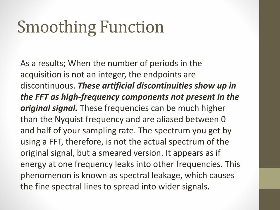
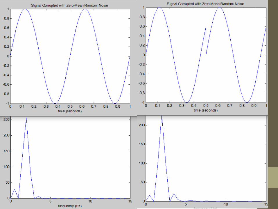
As a results; When the number of periods in the acquisition is not an integer, the endpoints are discontinuous. These artificial discontinuities show up in the FFT as high-frequency components not present in the original signal. These frequencies can be much higher than the Nyquist frequency and are aliased between 0 and half of your sampling rate. The spectrum you get by using a FFT, therefore, is not the actual spectrum of the original signal, but a smeared version. It appears as if energy at one frequency leaks into other frequencies. This phenomenon is known as spectral leakage, which causes the fine spectral lines to spread into wider signals.

Smoothing Function

Smoothing Function

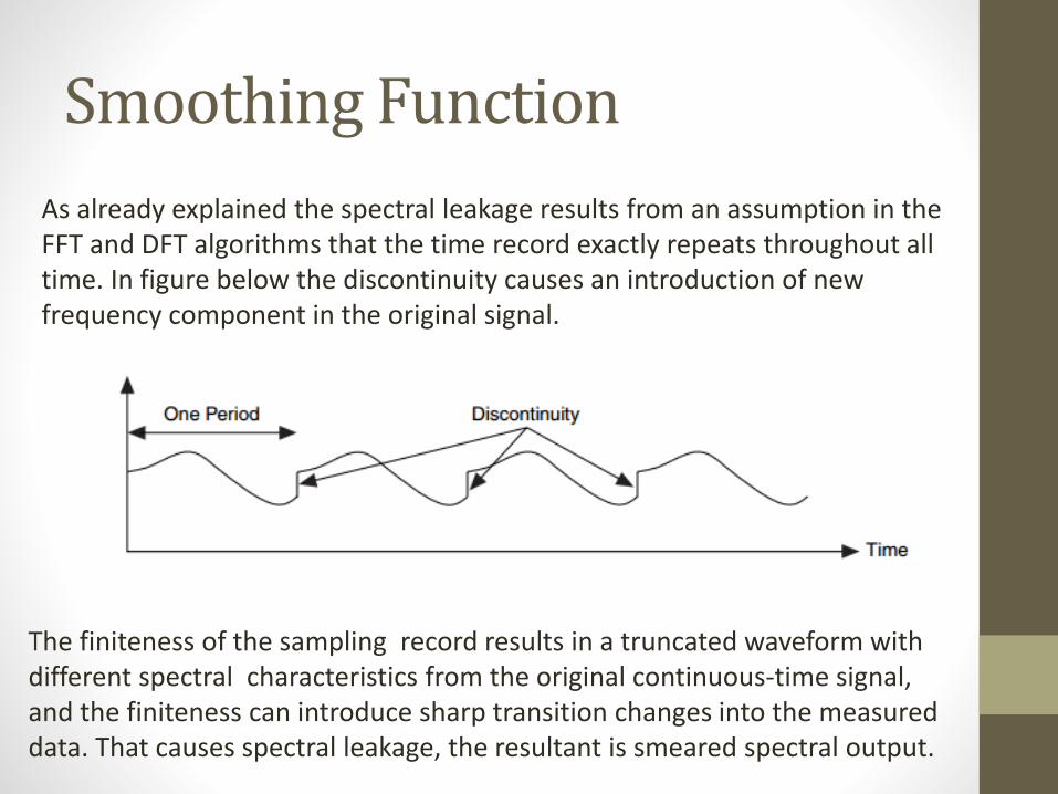
As already explained the spectral leakage results from an assumption in the FFT and DFT algorithms that the time record exactly repeats throughout all time. In figure below the discontinuity causes an introduction of new frequency component in the original signal.

The finiteness of the sampling record results in a truncated waveform with different spectral characteristics from the original continuous-time signal, and the finiteness can introduce sharp transition changes into the measured data. That causes spectral leakage, the resultant is smeared spectral output.

Smoothing Function: Discontinue Signal

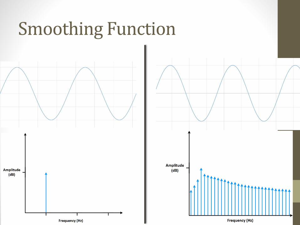
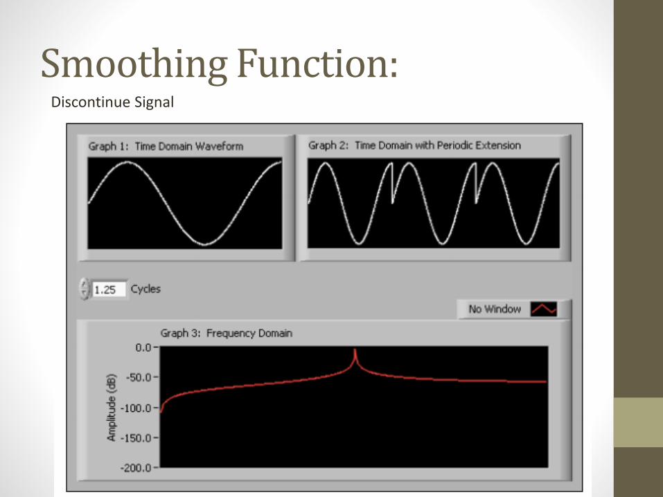
Graph 1 consists of 1.25 cycles of the sine wave. In Graph 2, the waveform repeats periodically to fulfill the assumption of periodicity for the Fourier transform. Graph 3 shows the spectral representation of the waveform. The energy is spread, or smeared, over a wide range of frequencies. The energy has leaked out of one of the FFT lines and smeared itself into all the other lines, causing spectral leakage.

Smoothing Function:

Smoothing Function

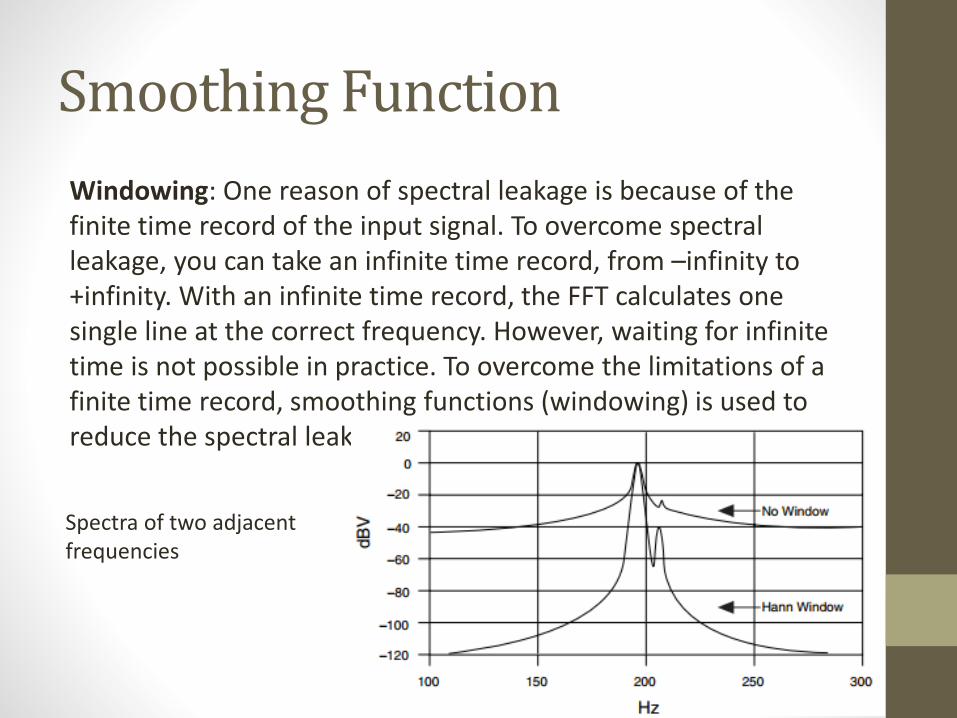
Windowing: One reason of spectral leakage is because of the finite time record of the input signal. To overcome spectral leakage, you can take an infinite time record, from –infinity to +infinity. With an infinite time record, the FFT calculates one single line at the correct frequency. However, waiting for infinite time is not possible in practice. To overcome the limitations of a finite time record, smoothing functions (windowing) is used to reduce the spectral leakage.

Spectra of two adjacent frequencies

Windowing Signal

Use smoothing windows to improve the spectral characteristics of a sampled signal. When performing Fourier or spectral analysis on finite-length data, you can use smoothing windows to minimize the discontinuities of truncated waveforms, thus reducing spectral leakage.

The amount of spectral leakage depends on the amplitude of the discontinuity. As the discontinuity becomes larger, spectral leakage increases, and vice versa. Smoothing windows reduce the amplitude of the discontinuities at the boundaries of each period and act like predefined, narrowband, lowpass filters.

Effect of Windowing

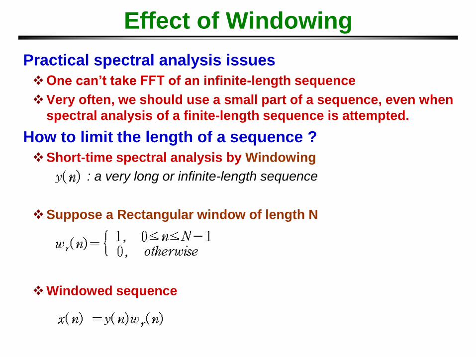
Practical spectral analysis issues

One can’t take FFT of an infinite-length sequence

Very often, we should use a small part of a sequence, even when

spectral analysis of a finite-length sequence is attempted.

How to limit the length of a sequence ?

Short-time spectral analysis by Windowing

Suppose a Rectangular window of length N

Windowed sequence

: a very long or infinite-length sequence

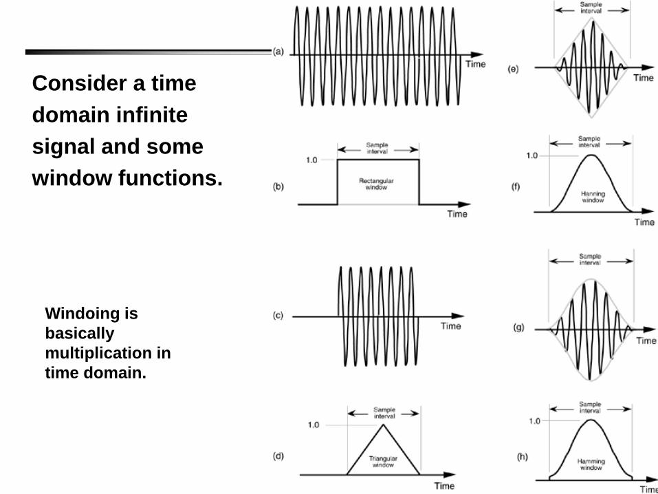
Consider a time

domain infinite

signal and some

window functions.

Windoing is

basically

multiplication in

time domain.

Important Parameters

Some of the more important properties of each window

function,

• Window shape

• Total energy

• Function

• Main lobe height

• Fraction of total energy E contained the ratio in (E0/E),

• Suppression of highest side lobe,

• Maximum scalloping.

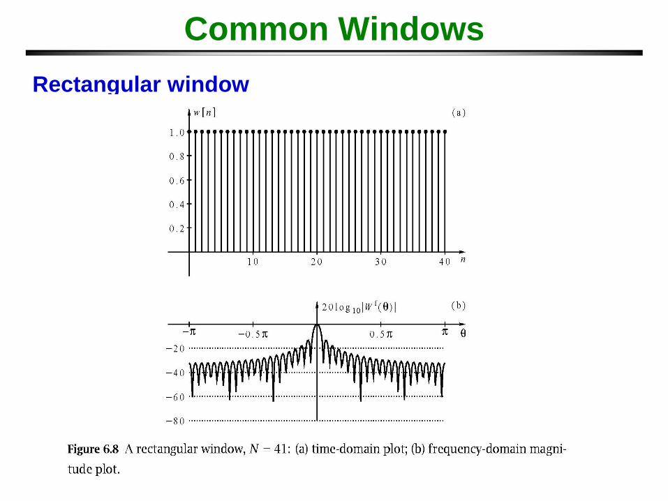
Common Windows

Rectangular window

Window function has it’s own spectra

Depending upon the level of energy, the spectra consists of a

main lobe and side lobes.

Main Lobe: To characterize the shape of the main lobe, the

width of the main lobe at –3 dB and –6 dB below the main lobe

peak describe the width of the main lobe. The unit of measure

for the main lobe width is FFT bins or frequency lines.

What happens actually???

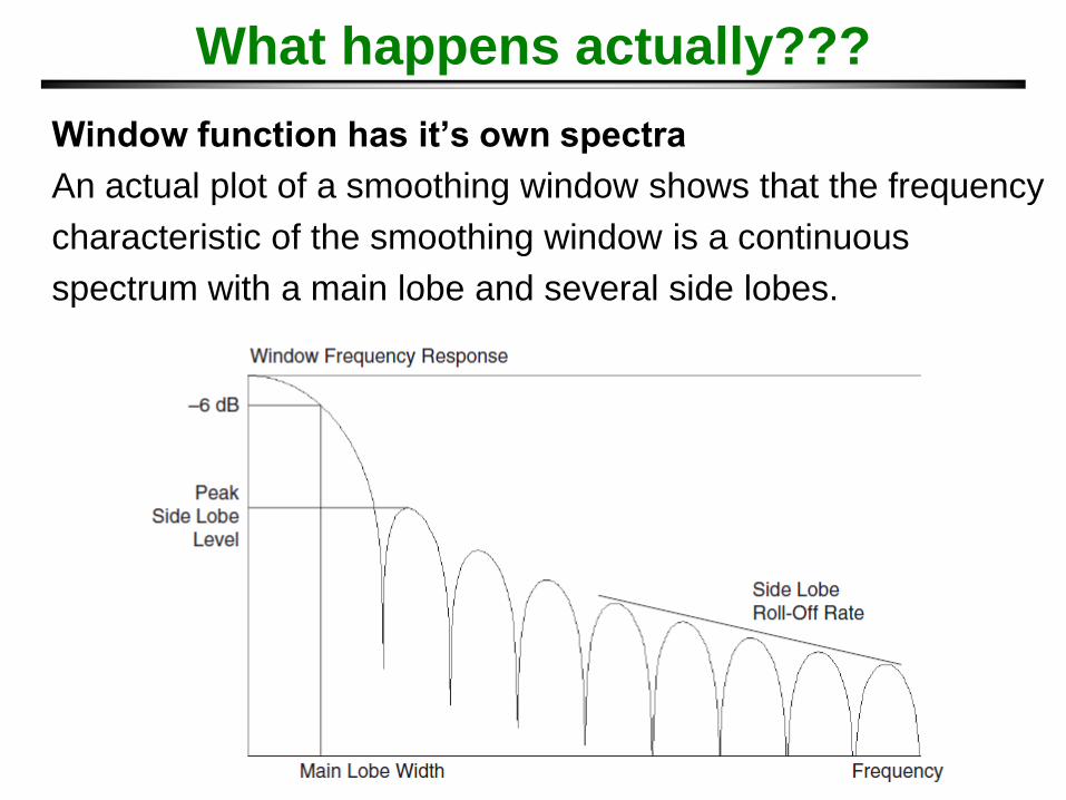
Window function has it’s own spectra

An actual plot of a smoothing window shows that the frequency

characteristic of the smoothing window is a continuous

spectrum with a main lobe and several side lobes.

What happens actually???

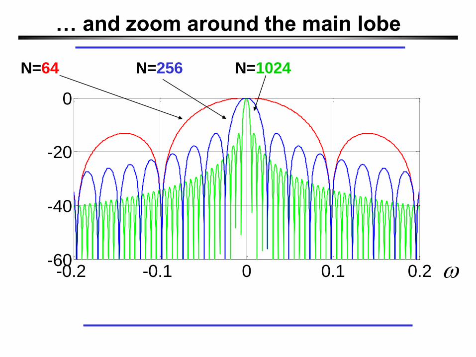
… and zoom around the main lobe

-0.2 -0.1 0 0.1 0.2-60

-40

-20

0

N=64 N=256 N=1024

w

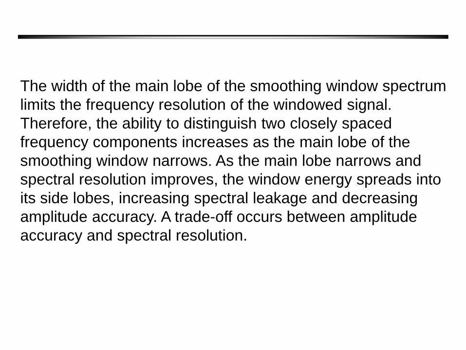
The width of the main lobe of the smoothing window spectrum

limits the frequency resolution of the windowed signal.

Therefore, the ability to distinguish two closely spaced

frequency components increases as the main lobe of the

smoothing window narrows. As the main lobe narrows and

spectral resolution improves, the window energy spreads into

its side lobes, increasing spectral leakage and decreasing

amplitude accuracy. A trade-off occurs between amplitude

accuracy and spectral resolution.

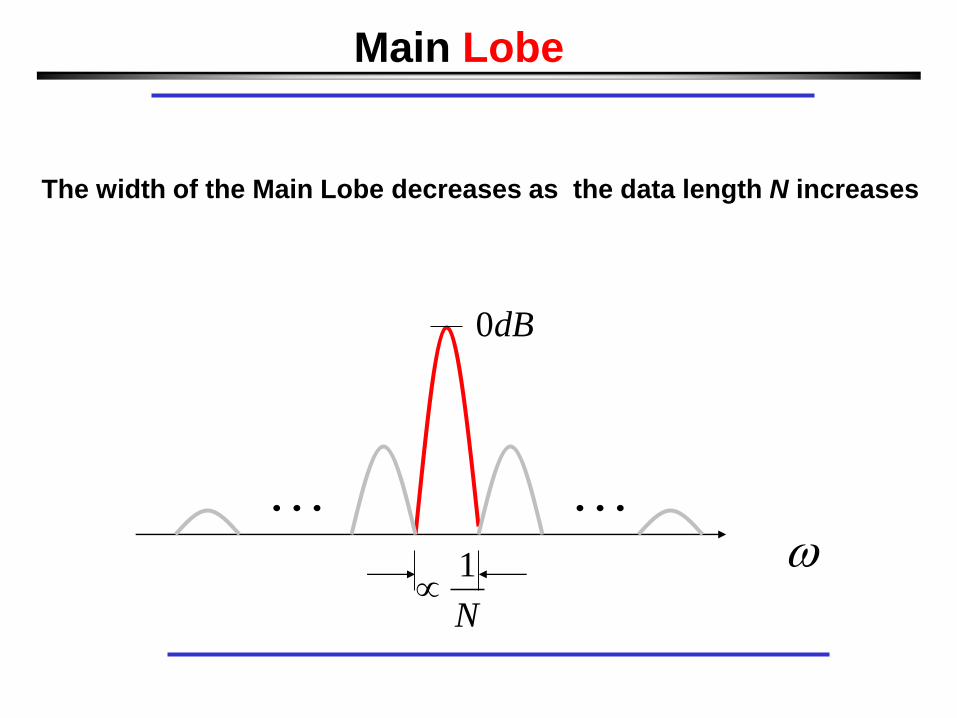
Main Lobe

The width of the Main Lobe decreases as the data length N increases

dB0

N

1

w

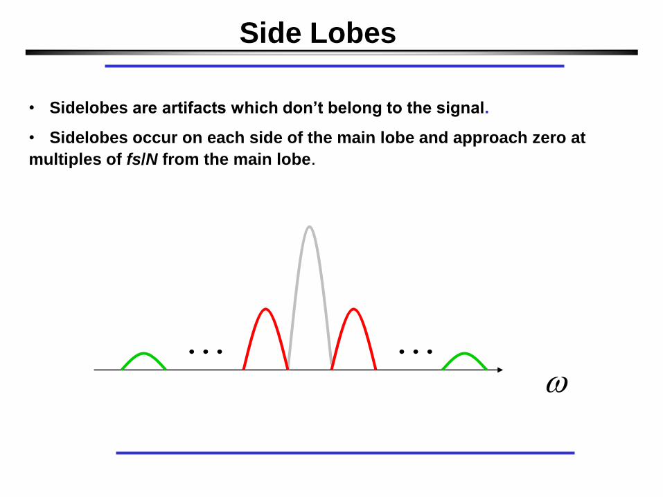
Side Lobes

• Sidelobes are artifacts which don’t belong to the signal.

• Sidelobes occur on each side of the main lobe and approach zero at

multiples of fs/N from the main lobe.

w

Types of Windows

Two types of windows

– Fixed: defined only by the duration of the window, N

– Parametric: have parameters that control the tradeoff

between main lobe width and side lobe amplitude

Common Windows: Fixed

Rectangular Window

The rectangular window has a value of one over its length. The

following equation defines the rectangular window.

w(n) = 1.0 for n = 0, 1, 2, …, N – 1

where N is the length of the window and w is the window

value.

Applying a rectangular window is equivalent to not using any

window because the rectangular function just truncates the

signal to within a finite time interval. The rectangular window

has the highest amount of spectral leakage.

Common Windows : Fixed

Rectangular Window

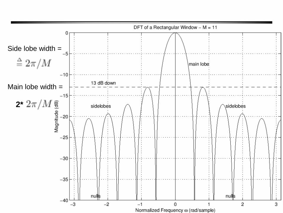
Side lobe width =

Main lobe width =

2*

Common Windows : Fixed

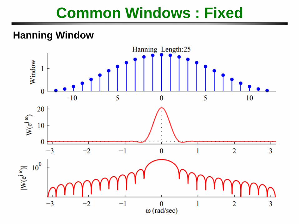
Hanning Window

The Hanning window has a shape similar to that of half a cycle

of a cosine wave. The following equation defines the Hanning

window.

where N is the length of the window and w is the window

value.

Common Windows : Fixed

Hanning Window

Common Windows : Fixed

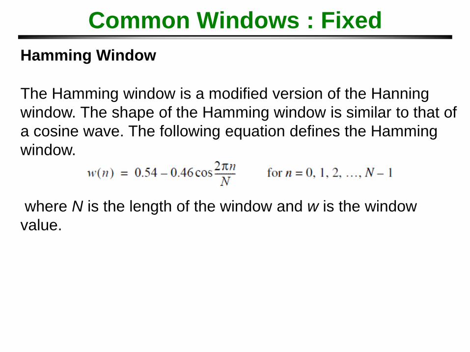
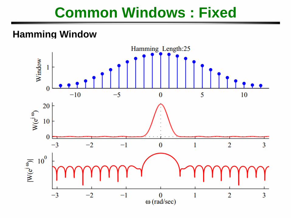
Hamming Window

The Hamming window is a modified version of the Hanning

window. The shape of the Hamming window is similar to that of

a cosine wave. The following equation defines the Hamming

window.

where N is the length of the window and w is the window

value.

Common Windows : Fixed

Hamming Window

Common Windows : Fixed

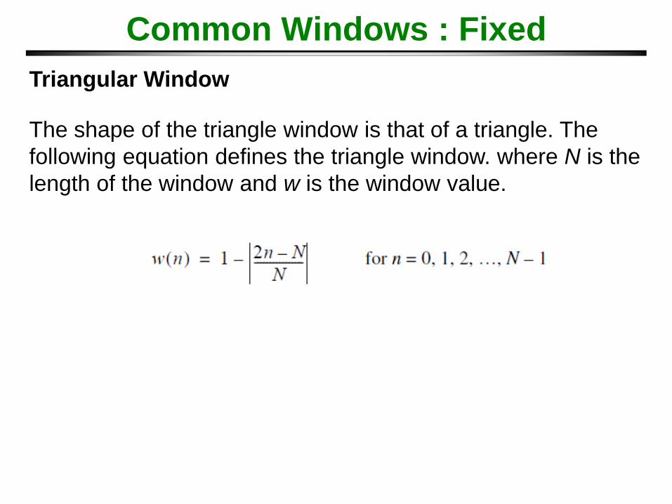
Triangular Window

The shape of the triangle window is that of a triangle. The

following equation defines the triangle window. where N is the

length of the window and w is the window value.

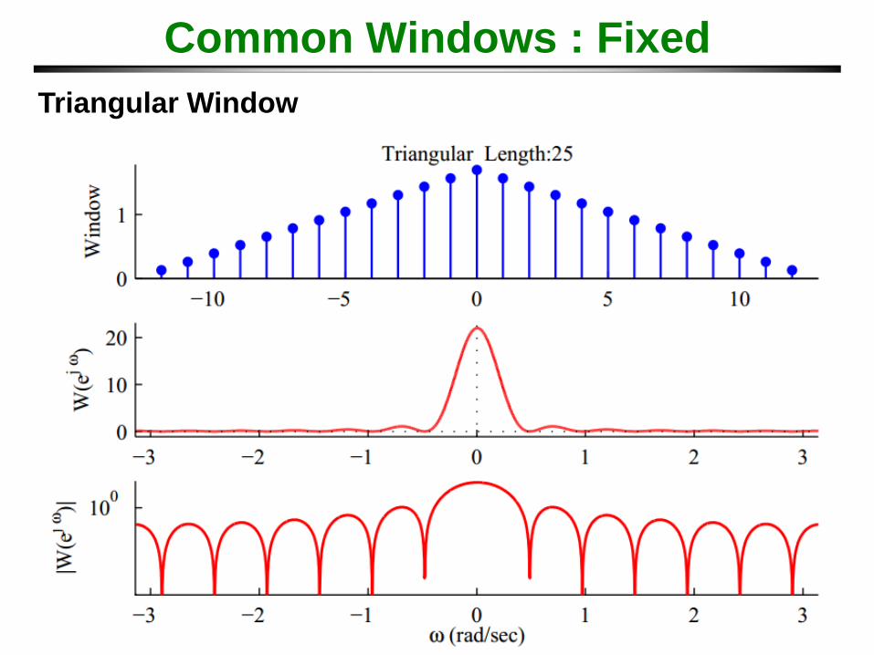
Common Windows : Fixed

Triangular Window

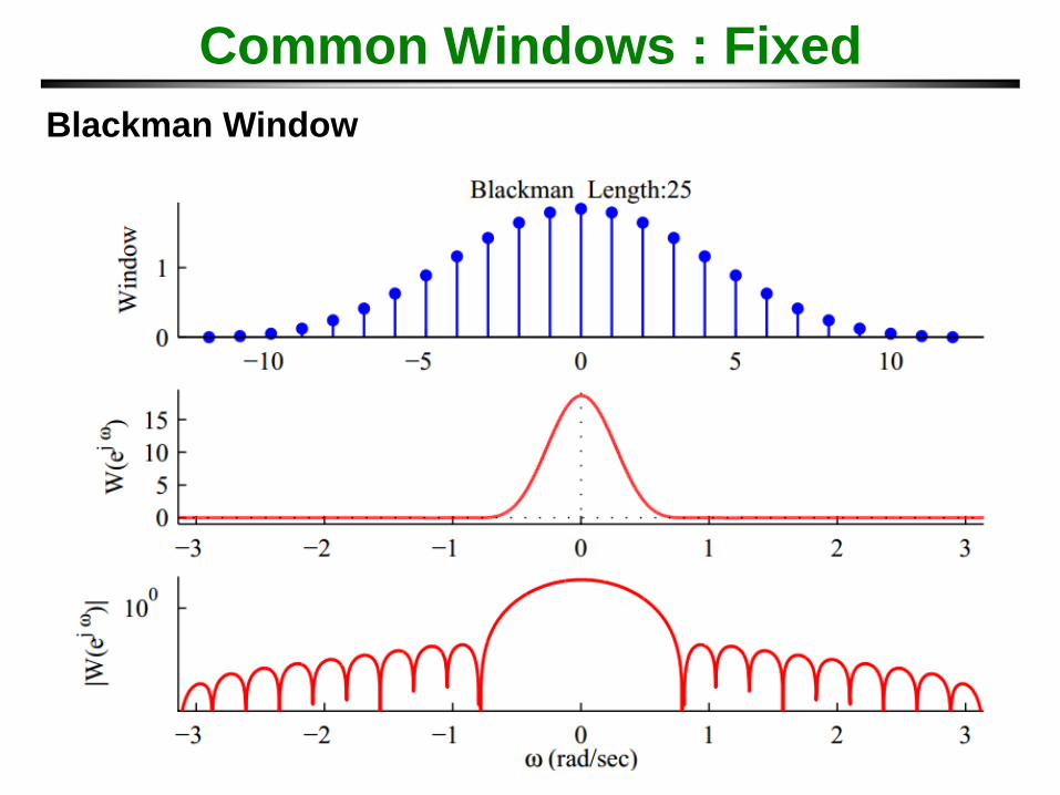
Common Windows : Fixed

Blackman Window

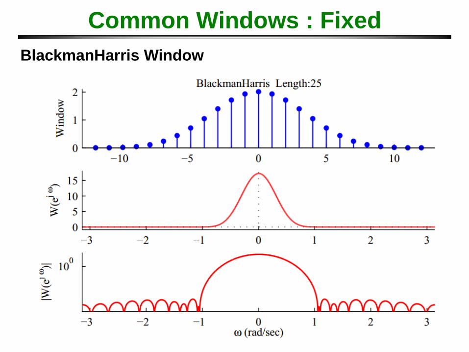
Common Windows : Fixed

BlackmanHarris Window

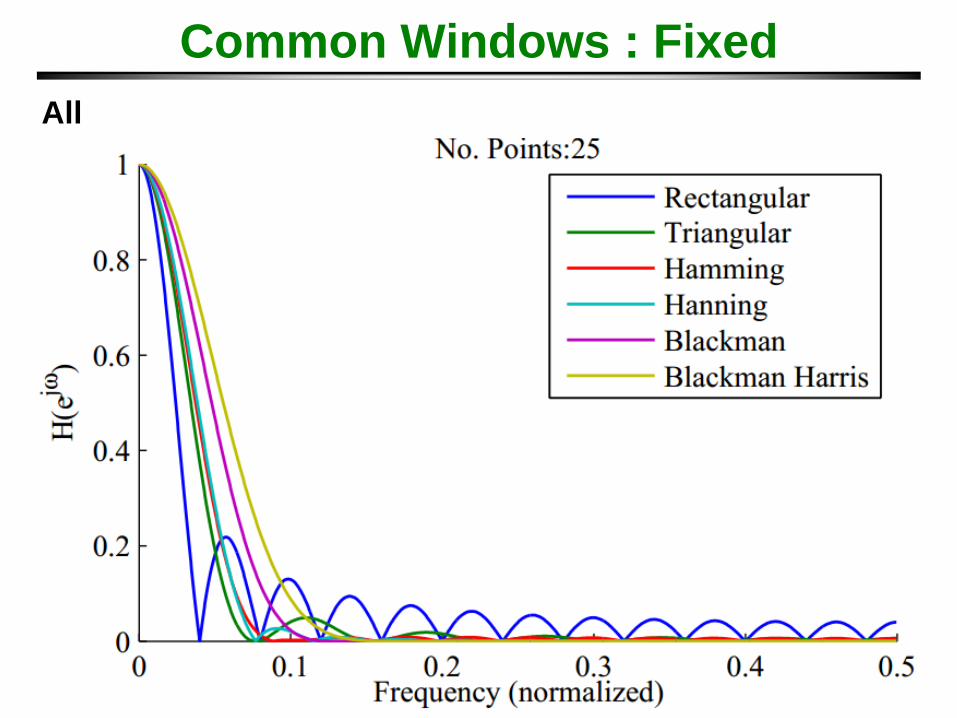
Common Windows : Fixed

All

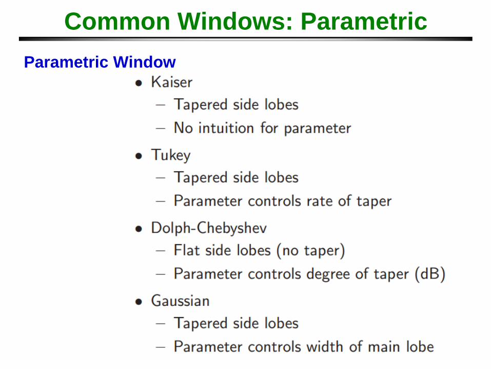
Common Windows: Parametric

Parametric Window

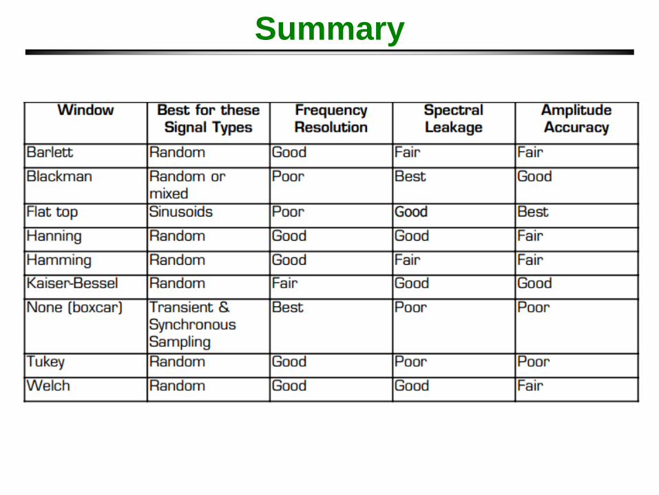
Summary

FFT windows reduce the effects of leakage but can not

eliminate leakage entirely. In effect, they only change the

shape of the leakage.

In addition, each type of window affects the spectrum in a

slightly different way. Each window has its own advantage and

disadvantage relative to the others. Some are more effective

for specific types of signal types such as random or

sinusoidal. Some improve the frequency resolution, that is,

they make it easier to detect the exact frequency of a peak in

the spectrum. Some improve the amplitude accuracy, that is,

they most accurately indicate the level of the peak. The best

type of window should be chosen for each specific application.

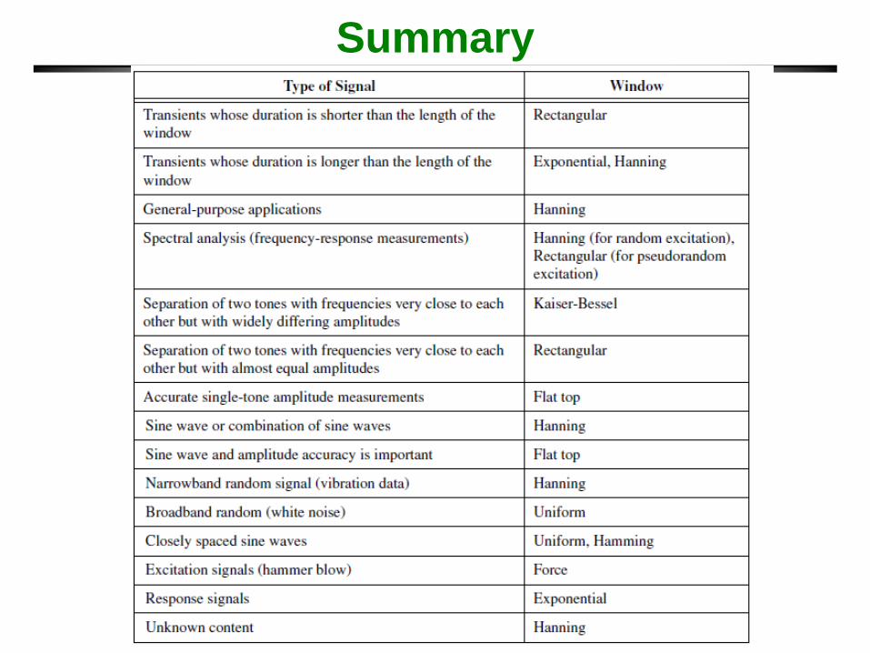
Summary

Choice of the window controls the tradeoff between

resolution and Side lobe leakage

• Rectangular window has maximum resolution and sidelobe

leakage

• Some windows have parameters that permit you to control

the tradeoff between resolution and leakage

• Best window depends on actual spectrum, usually the user

picks

• Ultimately, the window shape is much less important than

the duration of the window

• There is a much larger gain in accuracy by increasing N than

in picking the best window shape.

Smoothing windows

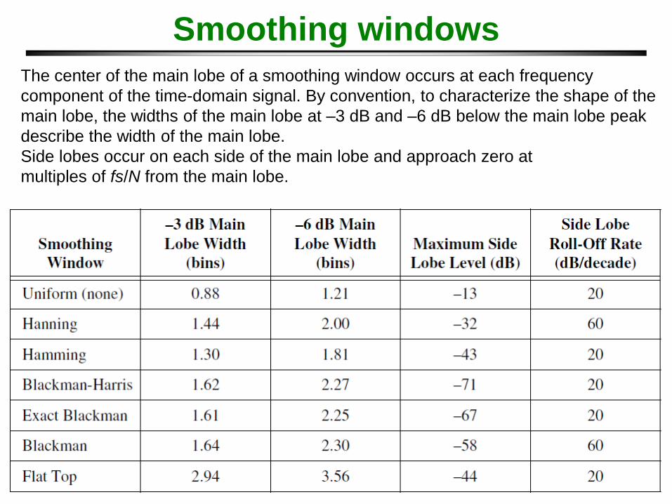
The center of the main lobe of a smoothing window occurs at each frequency

component of the time-domain signal. By convention, to characterize the shape of the

main lobe, the widths of the main lobe at –3 dB and –6 dB below the main lobe peak

describe the width of the main lobe.

Side lobes occur on each side of the main lobe and approach zero at

multiples of fs/N from the main lobe.

Summary

Summary

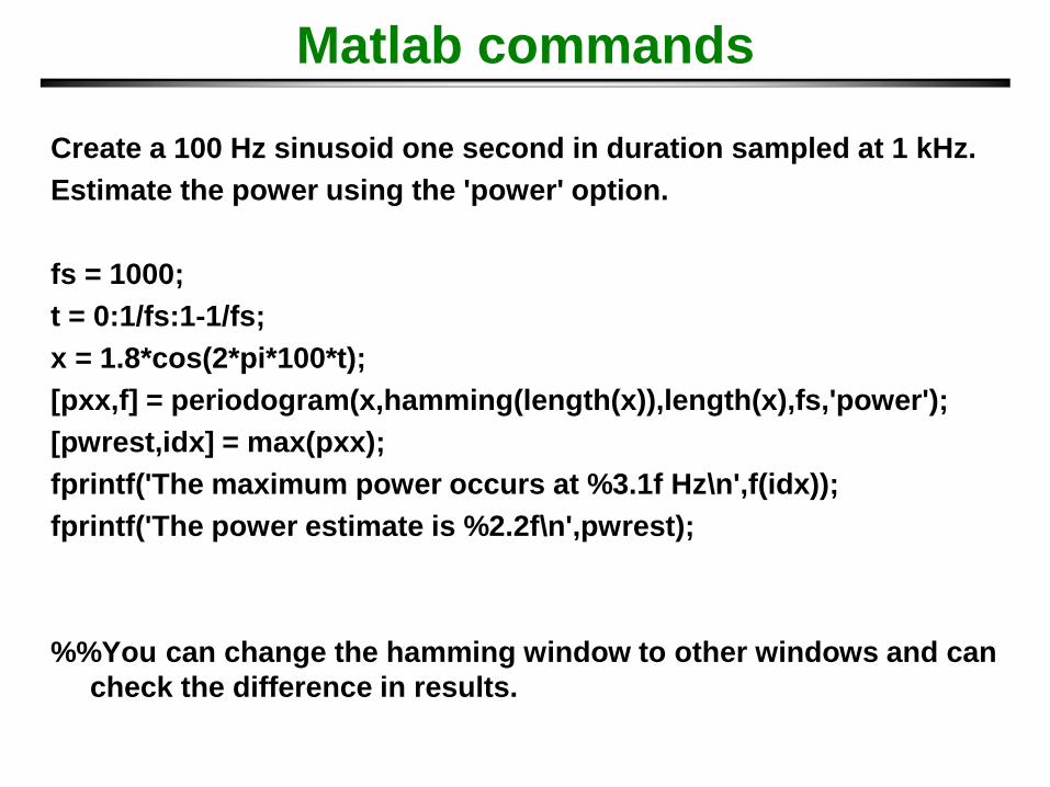
Matlab commands

Create a 100 Hz sinusoid one second in duration sampled at 1 kHz.

Estimate the power using the 'power' option.

fs = 1000;

t = 0:1/fs:1-1/fs;

x = 1.8*cos(2*pi*100*t);

[pxx,f] = periodogram(x,hamming(length(x)),length(x),fs,'power');

[pwrest,idx] = max(pxx);

fprintf('The maximum power occurs at %3.1f Hz\n',f(idx));

fprintf('The power estimate is %2.2f\n',pwrest);

%%You can change the hamming window to other windows and can

check the difference in results.

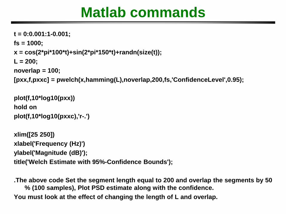
Matlab commands

t = 0:0.001:1-0.001;

fs = 1000;

x = cos(2*pi*100*t)+sin(2*pi*150*t)+randn(size(t));

L = 200;

noverlap = 100;

[pxx,f,pxxc] = pwelch(x,hamming(L),noverlap,200,fs,'ConfidenceLevel',0.95);

plot(f,10*log10(pxx))

hold on

plot(f,10*log10(pxxc),'r-.')

xlim([25 250])

xlabel('Frequency (Hz)')

ylabel('Magnitude (dB)');

title('Welch Estimate with 95%-Confidence Bounds');

.The above code Set the segment length equal to 200 and overlap the segments by 50

% (100 samples), Plot PSD estimate along with the confidence.

You must look at the effect of changing the length of L and overlap.

Digital Filtering

The filtering process alters the frequency

content of a signal.

Filter design is the process of creating the filter

coefficients to meet specific filtering requirements.

Filter implementation involves choosing and applying

a particular filter structure to those coefficients.

Only after both design and implementation have been

performed can data be filtered.

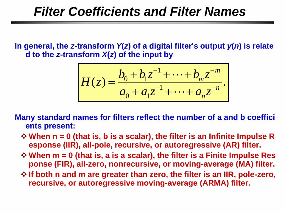
Filter Coefficients and Filter Names

In general, the z-transform Y(z) of a digital filter's output y(n) is related to the z-transform X(z) of the input by

Many standard names for filters reflect the number of a and b coefficients present:

When n = 0 (that is, b is a scalar), the filter is an Infinite Impulse Response (IIR), all-pole, recursive, or autoregressive (AR) filter.

When m = 0 (that is, a is a scalar), the filter is a Finite Impulse Response (FIR), all-zero, nonrecursive, or moving-average (MA) filter.

If both n and m are greater than zero, the filter is an IIR, pole-zero, recursive, or autoregressive moving-average (ARMA) filter.

.)(1

10

1

10

n

n

m

m

zazaa

zbzbbzH

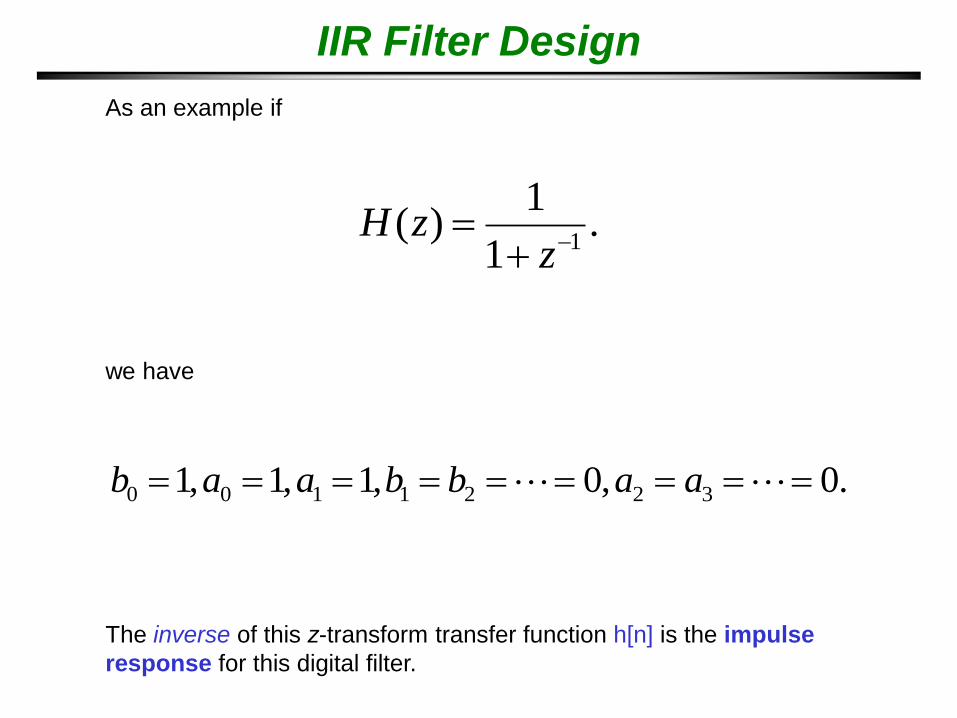
IIR Filter Design

As an example if

.1

1)(

1

zzH

.0,0,1,1,1 3221100 aabbaab

we have

The inverse of this z-transform transfer function h[n] is the impulse

response for this digital filter.

Digital Filtering

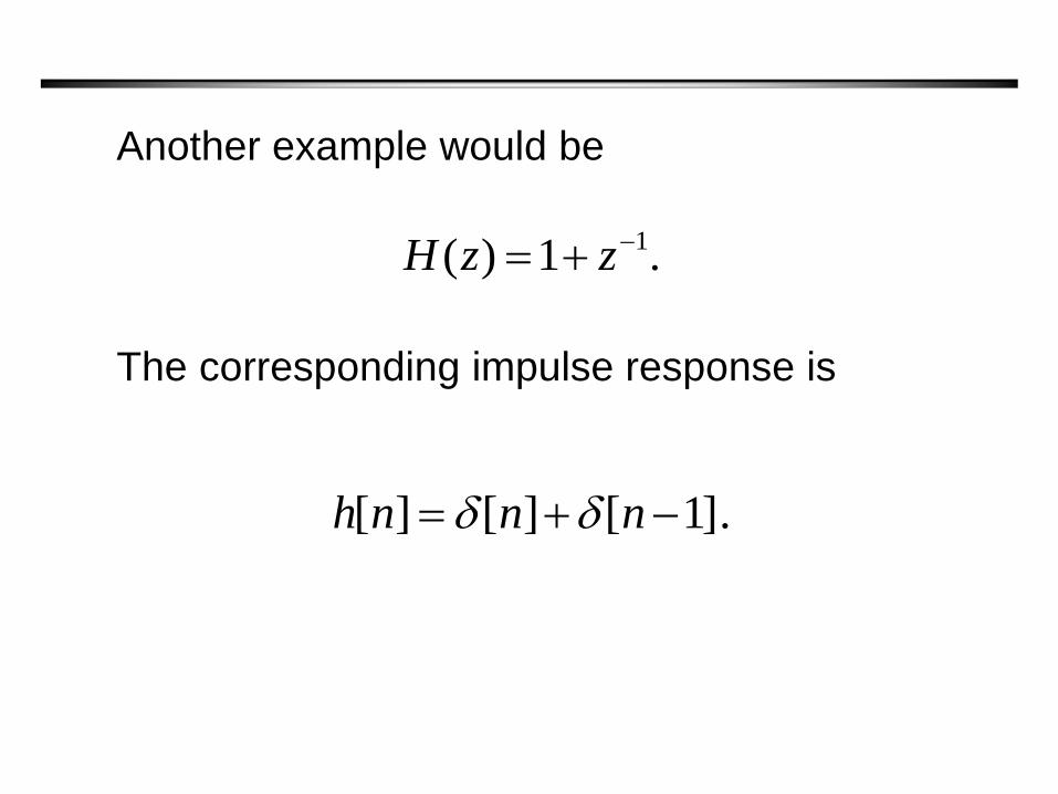
Another example would be

.1)( 1 zzH

The corresponding impulse response is

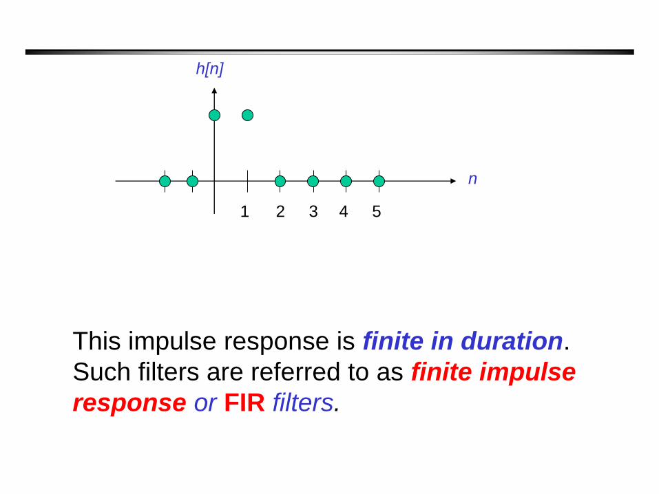
].1[][][ nnnh

1 2 3 4

n

h[n]

5

This impulse response is finite in duration.

Such filters are referred to as finite impulse

response or FIR filters.

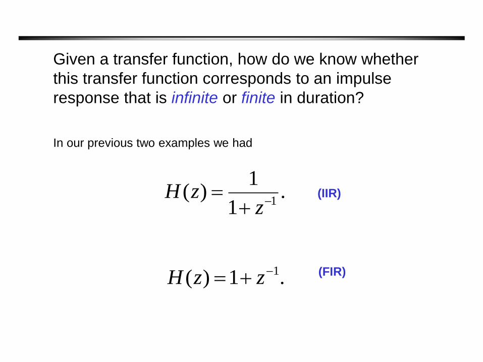
Given a transfer function, how do we know whether

this transfer function corresponds to an impulse

response that is infinite or finite in duration?

.1

1)(

1

zzH

.1)( 1 zzH

(IIR)

(FIR)

In our previous two examples we had

In general, any filter whose transfer function has a

denominator (that does not factor-out) will have an

impulse response that is infinite in duration

corresponding to an IIR filter.

Any filter whose transfer function does not have a

denominator will have an impulse response that is

finite in duration corresponding to an FIR filter.

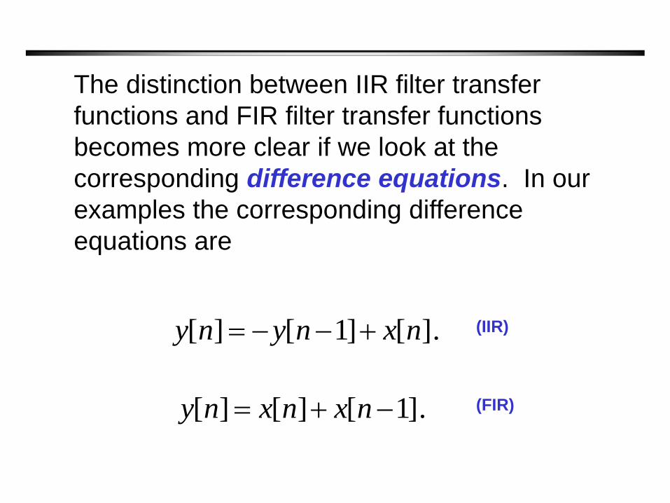
The distinction between IIR filter transfer

functions and FIR filter transfer functions

becomes more clear if we look at the

corresponding difference equations. In our

examples the corresponding difference

equations are

].1[][][ nxnxny

].[]1[][ nxnyny (IIR)

(FIR)

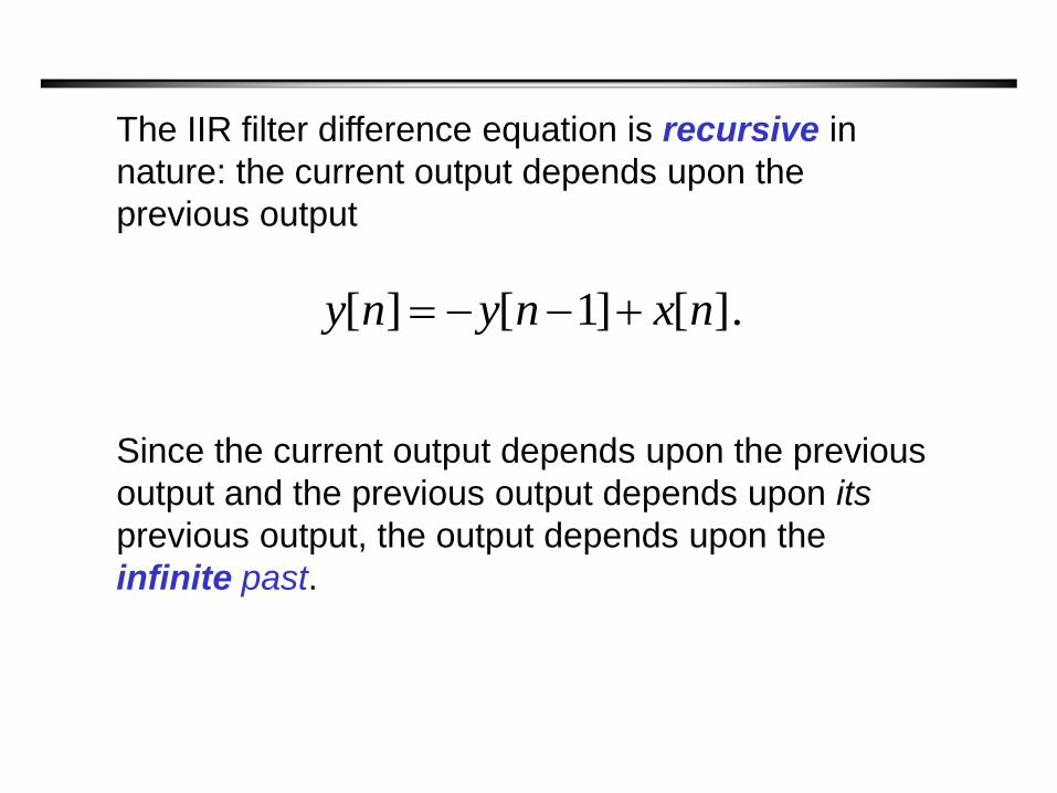
The IIR filter difference equation is recursive in

nature: the current output depends upon the

previous output

].[]1[][ nxnyny

Since the current output depends upon the previous

output and the previous output depends upon its

previous output, the output depends upon the

infinite past.

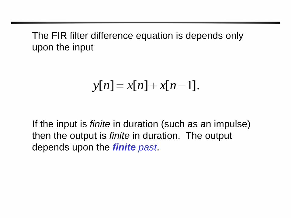
The FIR filter difference equation is depends only

upon the input

].1[][][ nxnxny

If the input is finite in duration (such as an impulse)

then the output is finite in duration. The output

depends upon the finite past.

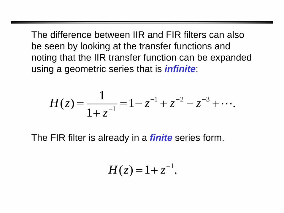
The difference between IIR and FIR filters can also

be seen by looking at the transfer functions and

noting that the IIR transfer function can be expanded

using a geometric series that is infinite:

.11

1)( 321

1

zzz

zzH

The FIR filter is already in a finite series form.

.1)( 1 zzH

Digital Filtering

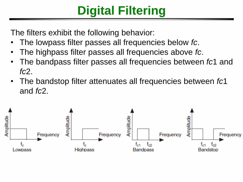
The filters exhibit the following behavior:

• The lowpass filter passes all frequencies below fc.

• The highpass filter passes all frequencies above fc.

• The bandpass filter passes all frequencies between fc1 and

fc2.

• The bandstop filter attenuates all frequencies between fc1

and fc2.

Digital Filtering

Ideally, Transition from pass band to stop band or

vice versa should take place in no-time.

A filter has a unit gain (0 dB) in the passband and a

gain of

zero (–∞ dB) in the stopband. However, real filters

cannot fulfill all the criteria of an ideal filter. In

practice, a finite transition band always exists

between the passband and the stopband. In the

transition band, the gain of the filter changes

gradually from one (0 dB) in the passband to

zero (–∞ dB) in the stopband.

Digital Filtering

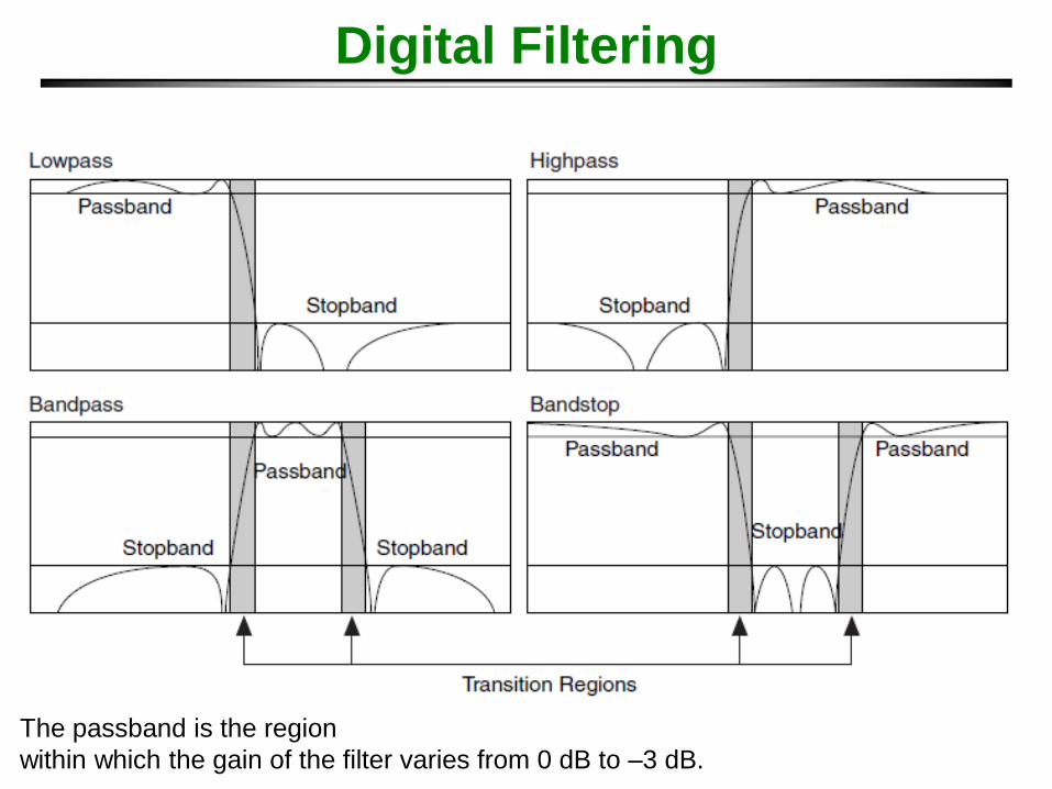
The passband is the region

within which the gain of the filter varies from 0 dB to –3 dB.

Digital Filtering: IIR

Digital Filtering: IIR

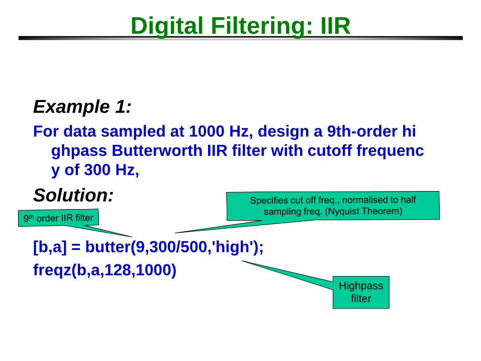
Example 1:

For data sampled at 1000 Hz, design a 9th-order hi

ghpass Butterworth IIR filter with cutoff frequenc

y of 300 Hz,

Solution:

[b,a] = butter(9,300/500,'high');

freqz(b,a,128,1000) Highpass

filter

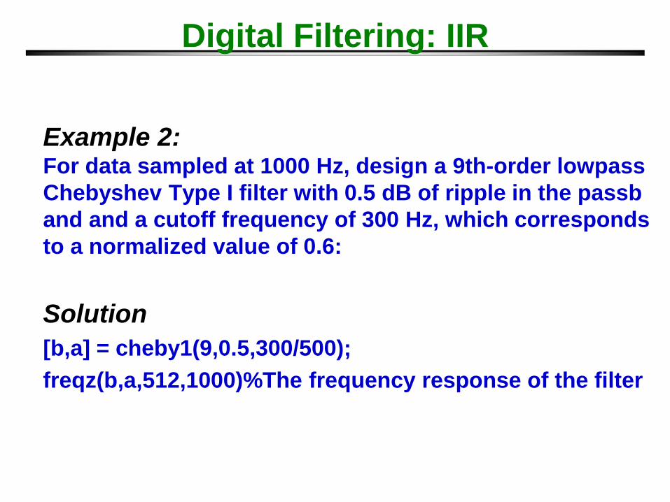
Example 2:For data sampled at 1000 Hz, design a 9th-order lowpass

Chebyshev Type I filter with 0.5 dB of ripple in the passb

and and a cutoff frequency of 300 Hz, which corresponds

to a normalized value of 0.6:

Solution

[b,a] = cheby1(9,0.5,300/500);

freqz(b,a,512,1000)%The frequency response of the filter

Digital Filtering: IIR