Embed Size (px)
Citation preview
Felix J. Herrmann*[email protected]
Joint work with Yogi Erlangga, and Tim Lin
*Seismic Laboratory for Imaging & ModelingDepartment of Earth & Ocean SciencesThe University of British Columbia
slim.eos.ubc.ca
Delphi, June 4th, 2009
Randomized wavefield inversion
Seismic Laboratory for Imaging and Modeling
Motivation Seismic data processing, modeling & inversion:
– firmly rooted in Nyquist’s sampling paradigm for (modeled) wavefields – too pessimistic for signals with structure– existence of sparsifying transforms (e.g. curvelets)
Major impediment: “curse of dimensionality”– acquisition >> processing & inversion >> modeling costs are proportional to the size of
data and image space
Solution strategy:– leverage new paradigm of compressive sensing (CS)
• identify simultaneous acquisition as CS• reduce acquisition, simulation, and inversion costs by randomization and
deliberate subsampling– recovery from sample rates ≈ computational cost proportional to transform-domain
sparsity of data or model
Seismic Laboratory for Imaging and Modeling
Today’s agenda Brief introduction to compressive sensing
– sparsifying transforms– randomized = incoherent downsampling– nonlinear recovery by sparsity promotion
Sparsity-promoting recovery from randomized simultaneous measurements
– missing separated shots versus missing simultaneous shots– recovery from simultaneous data with and without primary prediction (CSed EPSI)
Joint sparsity-promoting recovery from randomized image volumes– leverage focusing– reduction of model-space wavefields

Seismic Laboratory for Imaging and Modeling
Problem statementConsider the following (severely) underdetermined system of linear equations
Is it possible to recover x0 accurately from y?
unknown
data(measurements/observations/simulations)
x0
Ay=
Seismic Laboratory for Imaging and Modeling
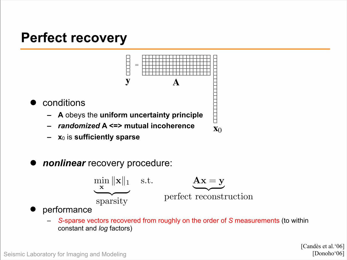
Perfect recovery
conditions– A obeys the uniform uncertainty principle– randomized A <=> mutual incoherence– x0 is sufficiently sparse
nonlinear recovery procedure:
performance– S-sparse vectors recovered from roughly on the order of S measurements (to within
constant and log factors)
minx
!x!1
! "# $
sparsity
s.t. Ax = y! "# $
perfect reconstruction
x0
Ay=
[Candès et al.‘06][Donoho‘06]
Seismic Laboratory for Imaging and Modeling
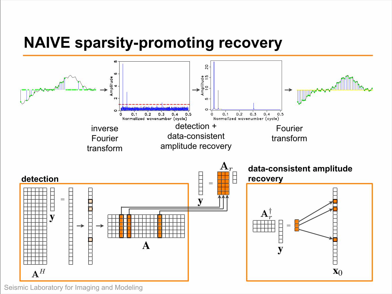
NAIVE sparsity-promoting recovery
inverseFourier
transform
detection +data-consistent
amplitude recovery
Fouriertransform
y
AH
=
A
y=detection
Ar data-consistent amplitude recovery
y
A†r
=
x0
Seismic Laboratory for Imaging and Modeling
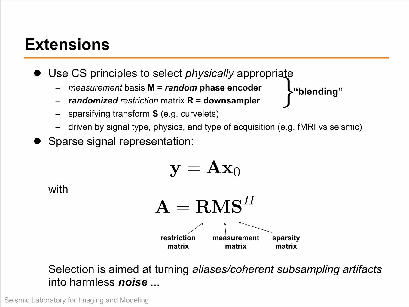
Extensions Use CS principles to select physically appropriate
– measurement basis M = random phase encoder– randomized restriction matrix R = downsampler– sparsifying transform S (e.g. curvelets)– driven by signal type, physics, and type of acquisition (e.g. fMRI vs seismic)
Sparse signal representation:
with
Selection is aimed at turning aliases/coherent subsampling artifacts into harmless noise ...
y = Ax0
A = RMSH
restrictionmatrix
measurementmatrix
sparsitymatrix
}“blending”
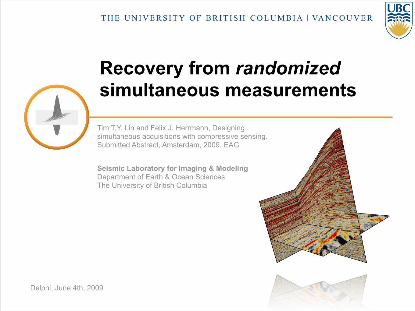
Tim T.Y. Lin and Felix J. Herrmann, Designing simultaneous acquisitions with compressive sensing. Submitted Abstract, Amsterdam, 2009, EAG
Seismic Laboratory for Imaging & ModelingDepartment of Earth & Ocean SciencesThe University of British Columbia
Delphi, June 4th, 2009
Recovery from randomized simultaneous measurements
Seismic Laboratory for Imaging and Modeling
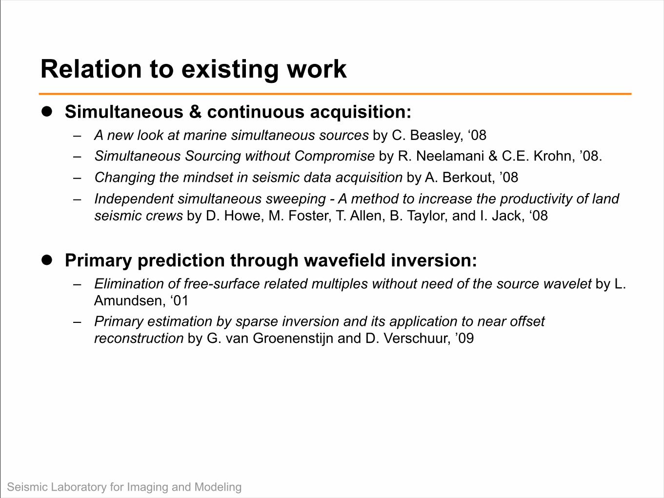
Relation to existing work Simultaneous & continuous acquisition:
– A new look at marine simultaneous sources by C. Beasley, ‘08– Simultaneous Sourcing without Compromise by R. Neelamani & C.E. Krohn, ’08.– Changing the mindset in seismic data acquisition by A. Berkout, ’08– Independent simultaneous sweeping - A method to increase the productivity of land
seismic crews by D. Howe, M. Foster, T. Allen, B. Taylor, and I. Jack, ‘08
Primary prediction through wavefield inversion:– Elimination of free-surface related multiples without need of the source wavelet by L.
Amundsen, ‘01– Primary estimation by sparse inversion and its application to near offset
reconstruction by G. van Groenenstijn and D. Verschuur, ’09

Seismic Laboratory for Imaging and Modeling
Two questions Question I: What is better? Having missing single-source or
missing randomized simultaneous experiments?
Comparison between different undersampling strategies for source experiments:
– Deterministic missing shot positions– Randomized jittered shot positions– Randomized simultaneous shots
Question II: What is better? First recover and then process or process directly in the compressed domain?
Example: randomized primary prediction with EPSI

Seismic Laboratory for Imaging and Modeling
Model

Seismic Laboratory for Imaging and Modeling
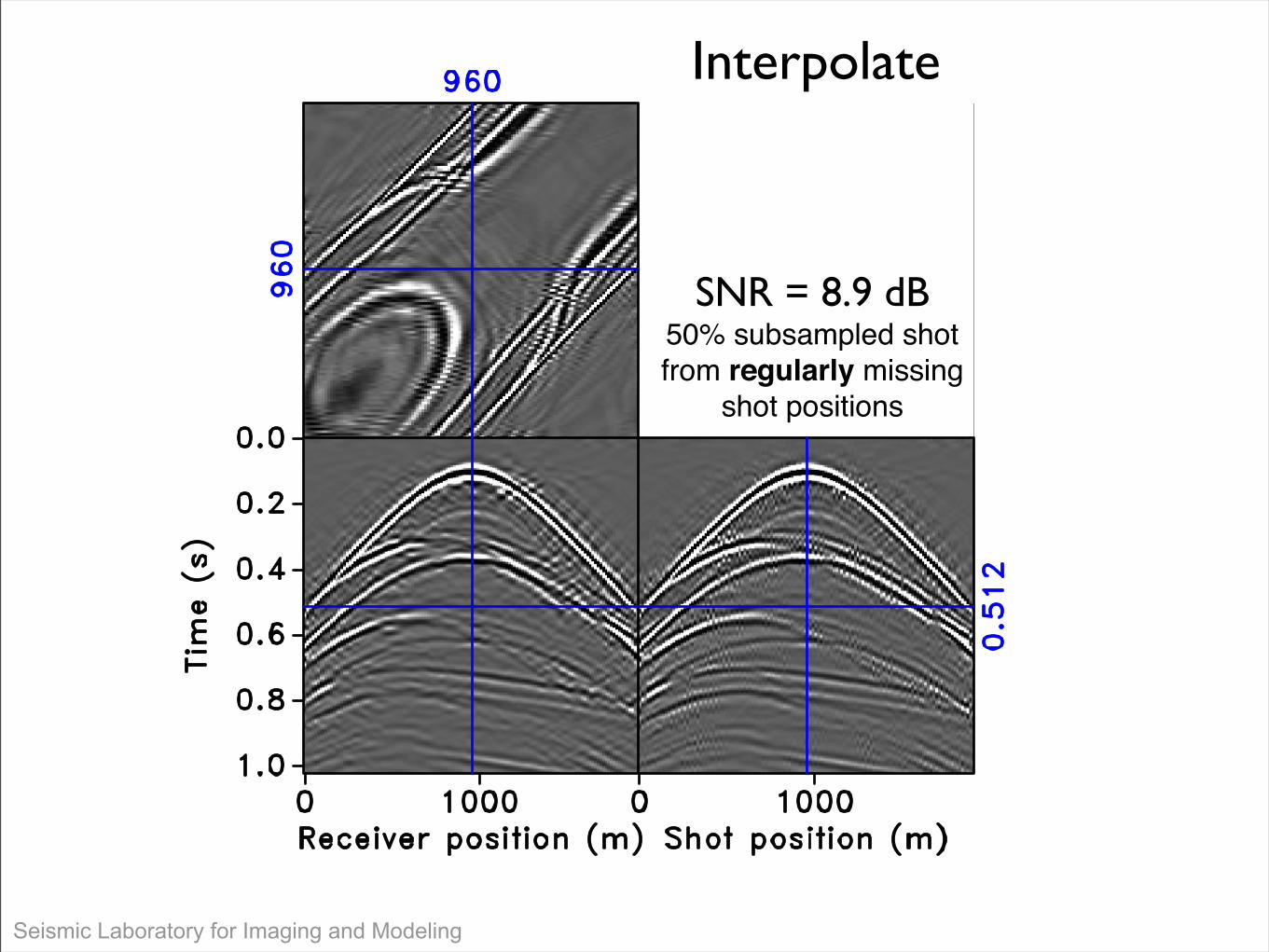
Interpolate
50% subsampled shotfrom regularly missing
shot positions
Seismic Laboratory for Imaging and Modeling
Interpolate
SNR = 8.9 dB50% subsampled shotfrom regularly missing
shot positions

Seismic Laboratory for Imaging and Modeling
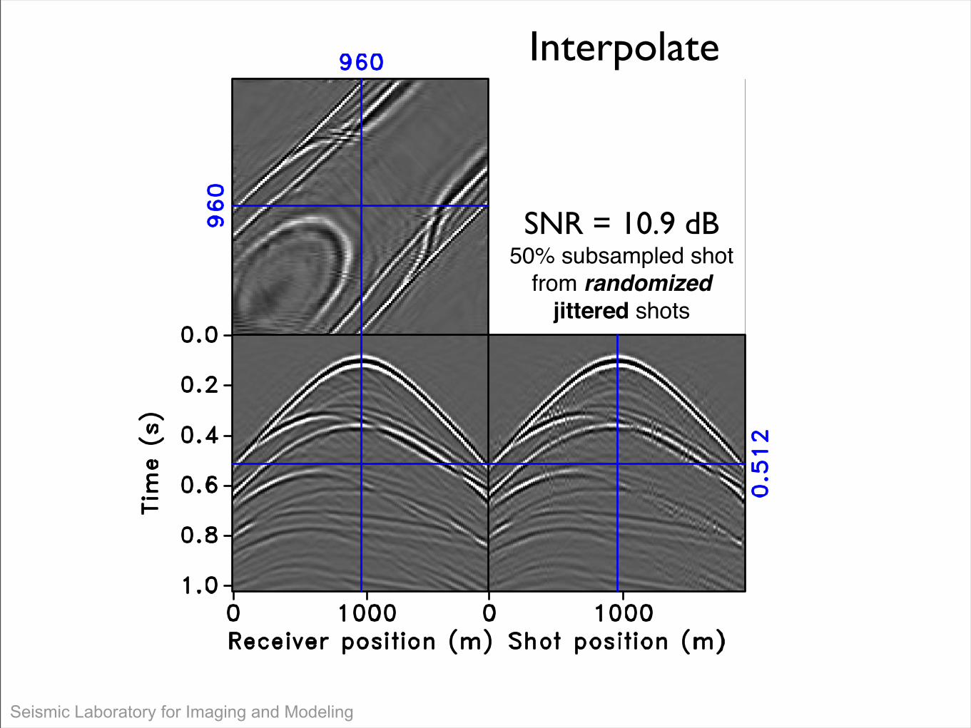
Interpolate
50% subsampled shot
from randomized jittered shots
Seismic Laboratory for Imaging and Modeling
Interpolate
SNR = 10.9 dB50% subsampled shot
from randomized jittered shots
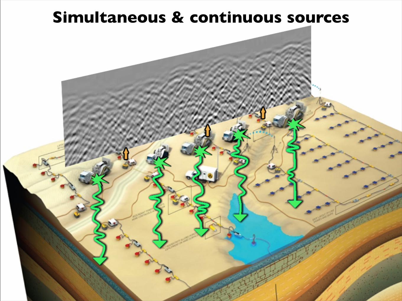
Simultaneous & continuous sources
Seismic Laboratory for Imaging and Modeling
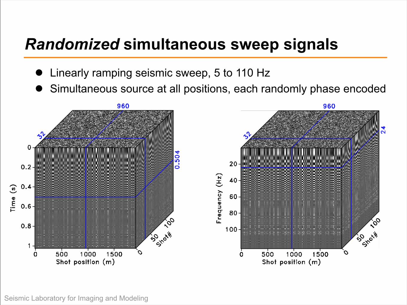
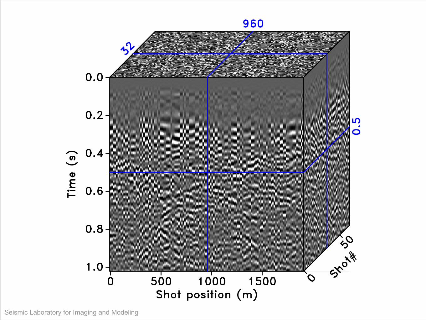
Linearly ramping seismic sweep, 5 to 110 Hz Simultaneous source at all positions, each randomly phase encoded
Randomized simultaneous sweep signals
Seismic Laboratory for Imaging and Modeling
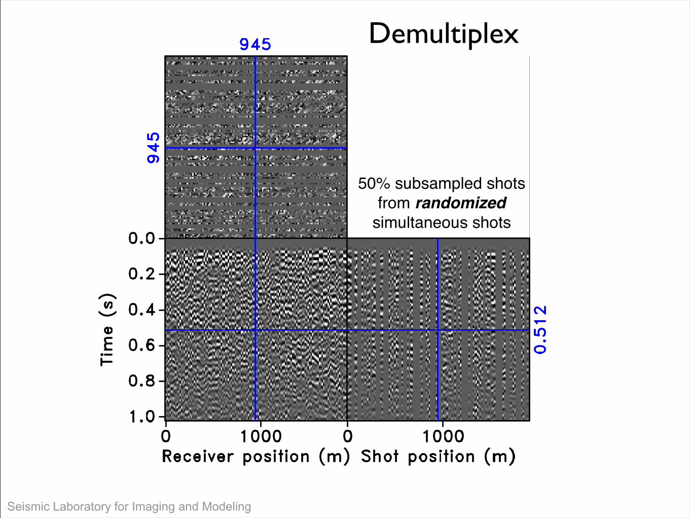
Demultiplex
50% subsampled shots
from randomizedsimultaneous shots

Seismic Laboratory for Imaging and Modeling
Demultiplex
SNR = 16.1 dB50% subsampled shot
from randomizedsimultaneous shots
Seismic Laboratory for Imaging and Modeling
Seismic Laboratory for Imaging and Modeling
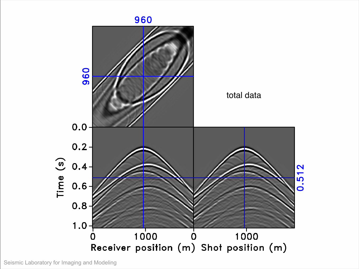
total data

Seismic Laboratory for Imaging and Modeling
Primary-prediction from
randomizedcompressive data
Seismic Laboratory for Imaging and Modeling
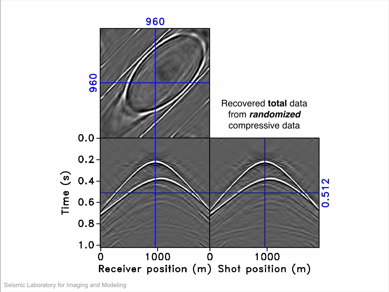
Recovered total data
from randomizedcompressive data
Seismic Laboratory for Imaging and Modeling
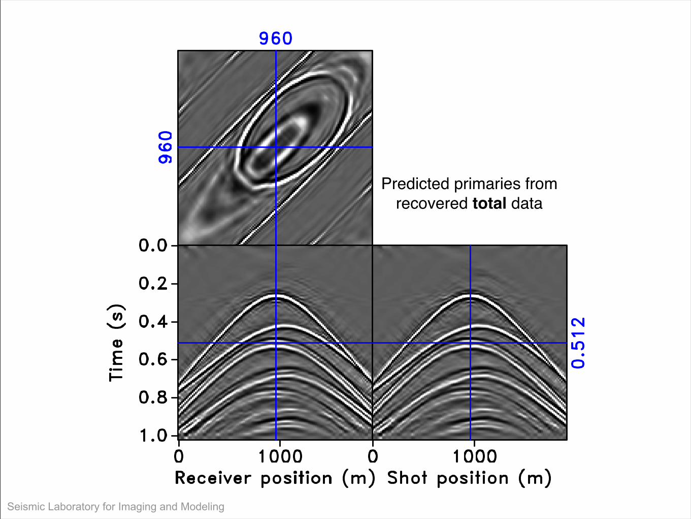
Predicted primaries from
recovered total data

Seismic Laboratory for Imaging and Modeling
Observations Incoherent randomized sampling crucial for creating favorable
recovery conditions for sparsity-promoting recovery from “incomplete” data
– depends on the choice of downsampled randomization RM– simultaneous acquisition is better for reconstruction
Recovery greatly improves when estimating primaries– deconvolved primaries are sparser than multiples– multiples are mapped to primaries– example of randomized wavefield inversion with reduced sizes
Push recovery down into processing flow, i.e., compressive processing & imaging
Extend these ideas to imaging = model-space compressive sampling
Felix J. Herrmann, Compressive imaging by wavefield inversion with group sparsity. Submitted abstract, SEG, 2009, Houston. Technical Report TR-2009-01
Seismic Laboratory for Imaging & ModelingDepartment of Earth & Ocean SciencesThe University of British Columbia
Delphi, June 4th, 2009
Recovery from randomized image volumes
Seismic Laboratory for Imaging and Modeling
Strategy Leverage CS towards solutions of wave simulation & imaging
problems
Subsample solution deliberately, followed by CS recovery
Speedup if recovery costs < gain in reduced system size– computation– storage
Examples:– compressed imaging by CS sampling in the model space
Seismic Laboratory for Imaging and Modeling
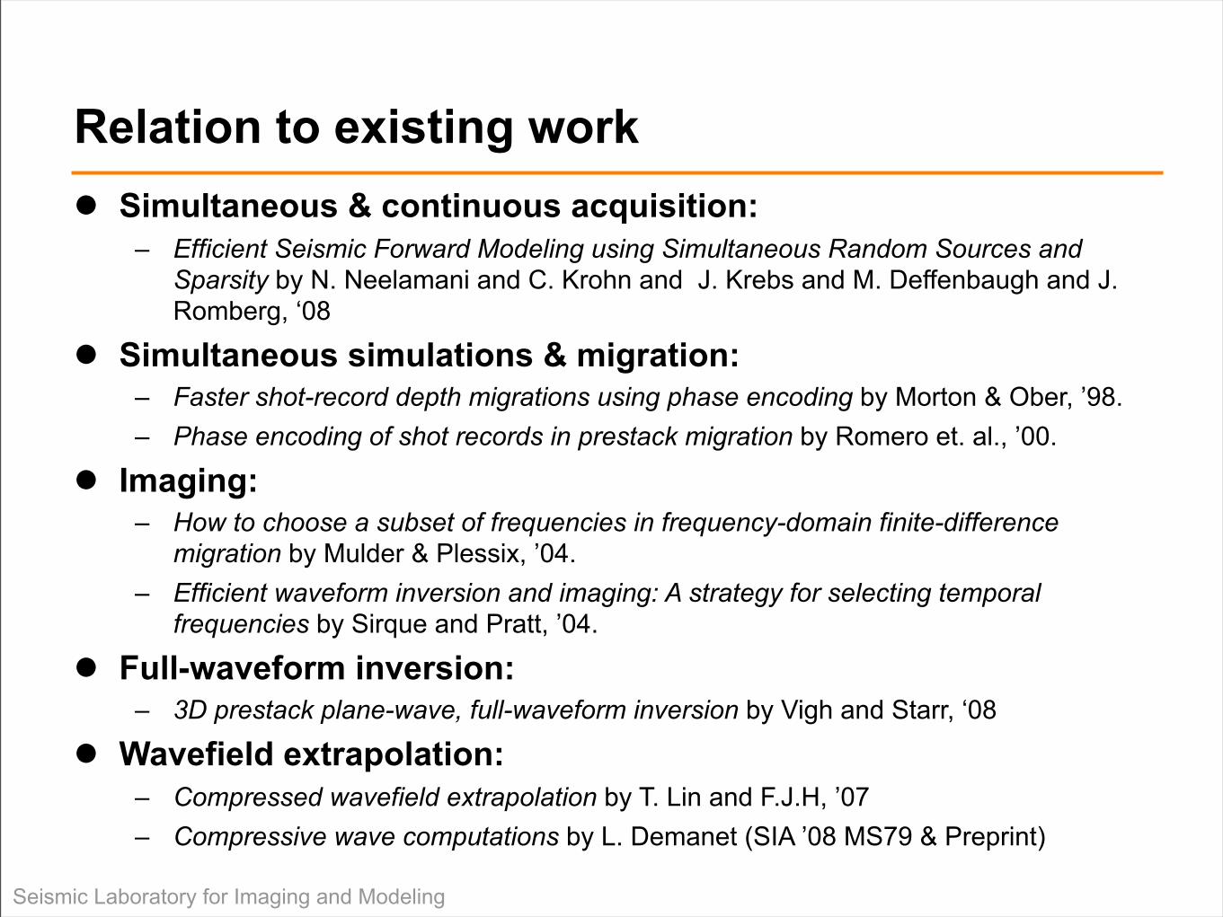
Relation to existing work Simultaneous & continuous acquisition:
– Efficient Seismic Forward Modeling using Simultaneous Random Sources and Sparsity by N. Neelamani and C. Krohn and J. Krebs and M. Deffenbaugh and J. Romberg, ‘08
Simultaneous simulations & migration:– Faster shot-record depth migrations using phase encoding by Morton & Ober, ’98.– Phase encoding of shot records in prestack migration by Romero et. al., ’00.
Imaging:– How to choose a subset of frequencies in frequency-domain finite-difference
migration by Mulder & Plessix, ’04.– Efficient waveform inversion and imaging: A strategy for selecting temporal
frequencies by Sirque and Pratt, ’04.
Full-waveform inversion:– 3D prestack plane-wave, full-waveform inversion by Vigh and Starr, ‘08
Wavefield extrapolation:– Compressed wavefield extrapolation by T. Lin and F.J.H, ’07– Compressive wave computations by L. Demanet (SIA ’08 MS79 & Preprint)
Seismic Laboratory for Imaging and Modeling
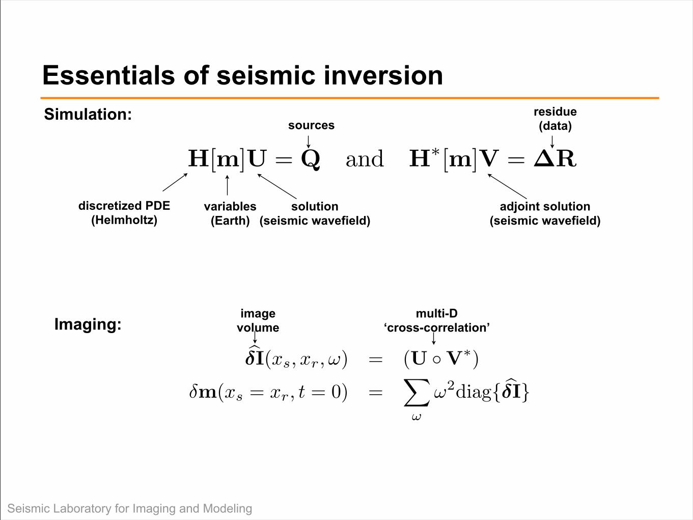
Essentials of seismic inversion
discretized PDE(Helmholtz)
variables(Earth)
solution(seismic wavefield)
sources
adjoint solution(seismic wavefield)
residue (data)
Simulation:
imagevolume
multi-D ‘cross-correlation’Imaging:
H[m]U = Q and H![m]V = !R
!!I(xs, xr,!) = (U ! V!)
"m(xs = xr, t = 0) ="
!
!2diag{ !!I}
Seismic Laboratory for Imaging and Modeling
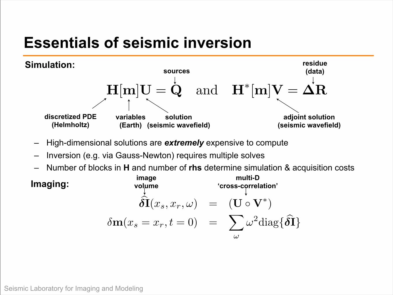
Essentials of seismic inversion
– High-dimensional solutions are extremely expensive to compute– Inversion (e.g. via Gauss-Newton) requires multiple solves– Number of blocks in H and number of rhs determine simulation & acquisition costs
discretized PDE(Helmholtz)
variables(Earth)
solution(seismic wavefield)
sources
adjoint solution(seismic wavefield)
residue (data)
Simulation:
imagevolume
multi-D ‘cross-correlation’Imaging:
H[m]U = Q and H![m]V = !R
!!I(xs, xr,!) = (U ! V!)
"m(xs = xr, t = 0) ="
!
!2diag{ !!I}
Seismic Laboratory for Imaging and Modeling
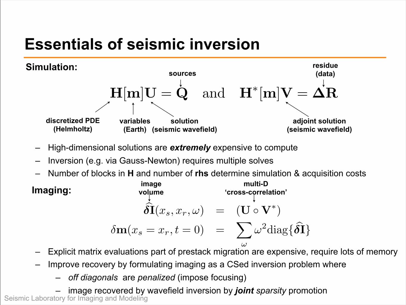
Essentials of seismic inversion
– High-dimensional solutions are extremely expensive to compute– Inversion (e.g. via Gauss-Newton) requires multiple solves– Number of blocks in H and number of rhs determine simulation & acquisition costs
discretized PDE(Helmholtz)
variables(Earth)
solution(seismic wavefield)
sources
adjoint solution(seismic wavefield)
residue (data)
Simulation:
imagevolume
multi-D ‘cross-correlation’Imaging:
– Explicit matrix evaluations part of prestack migration are expensive, require lots of memory– Improve recovery by formulating imaging as a CSed inversion problem where
– off diagonals are penalized (impose focusing)– image recovered by wavefield inversion by joint sparsity promotion
H[m]U = Q and H![m]V = !R
!!I(xs, xr,!) = (U ! V!)
"m(xs = xr, t = 0) ="
!
!2diag{ !!I}
Seismic Laboratory for Imaging and Modeling
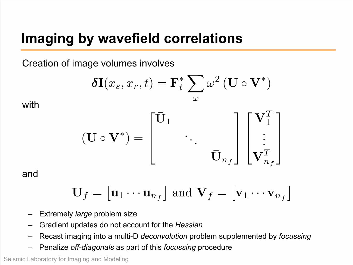
Imaging by wavefield correlationsCreation of image volumes involves
with
and
– Extremely large problem size– Gradient updates do not account for the Hessian– Recast imaging into a multi-D deconvolution problem supplemented by focussing– Penalize off-diagonals as part of this focussing procedure
!I(xs, xr, t) = F!t
!
!
!2 (U ! V!)
(U ! V!) =
!
"#U1
. . .Unf
$
%&
!
"#VT
1...
VTnf
$
%&
Uf =!u1 · · · unf
"and Vf =
!v1 · · · vnf
"
Seismic Laboratory for Imaging and Modeling
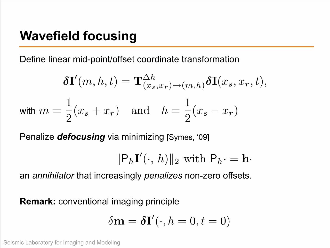
Wavefield focusingDefine linear mid-point/offset coordinate transformation
with
Penalize defocusing via minimizing [Symes, ‘09]
an annihilator that increasingly penalizes non-zero offsets.
Remark: conventional imaging principle
!I!(m,h, t) = T!h(xs,xr) "#(m,h)!I(xs, xr, t),
m =12(xs + xr) and h =
12(xs ! xr)
!PhI!(·, h)!2 with Ph· = h·
!m = !I!(·, h = 0, t = 0)
Seismic Laboratory for Imaging and Modeling
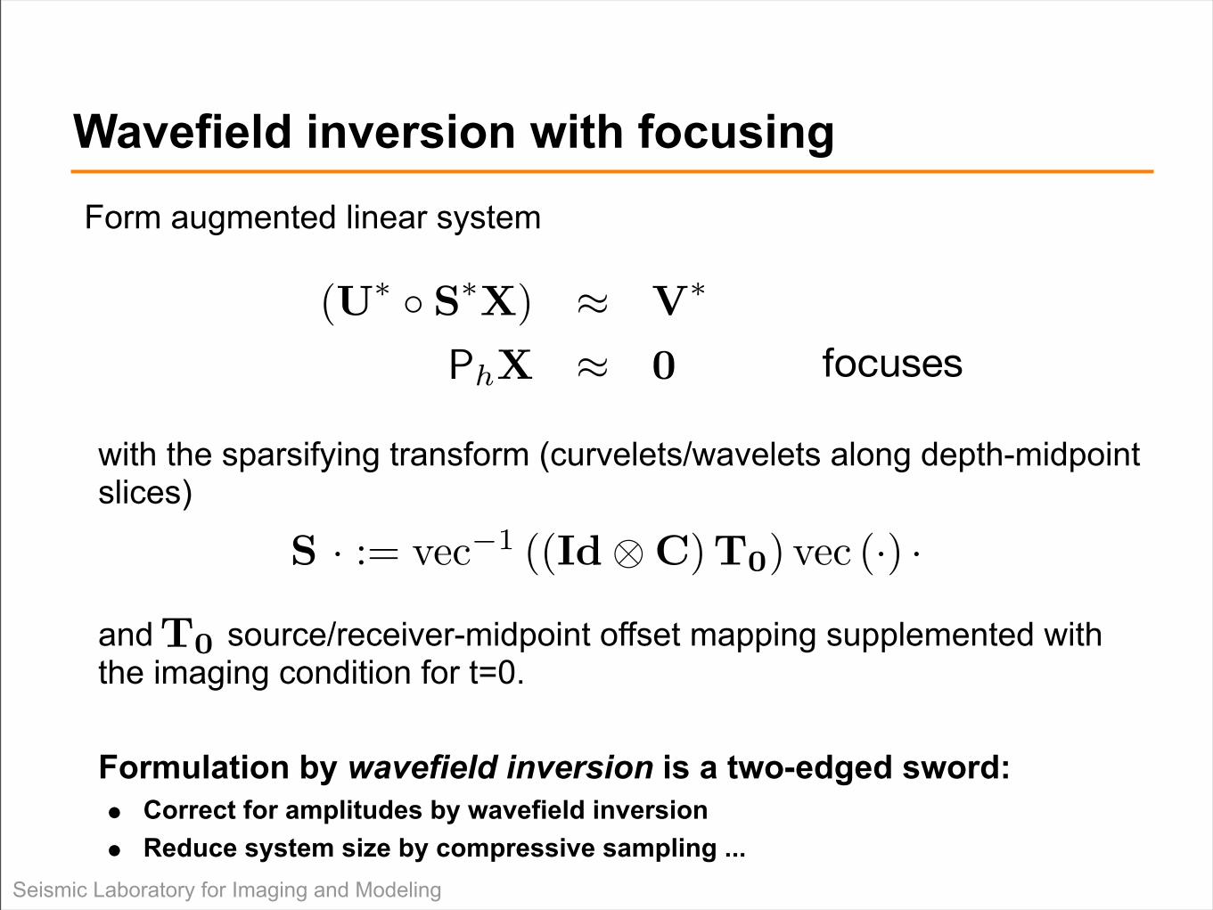
Wavefield inversion with focusing Form augmented linear system
with the sparsifying transform (curvelets/wavelets along depth-midpoint slices)
and source/receiver-midpoint offset mapping supplemented with the imaging condition for t=0.
Formulation by wavefield inversion is a two-edged sword:• Correct for amplitudes by wavefield inversion• Reduce system size by compressive sampling ...
focuses
T0
S · := vec!1 ((Id!C)T0) vec (·) ·
(U! ! S!X) " V!
PhX " 0
Seismic Laboratory for Imaging and Modeling
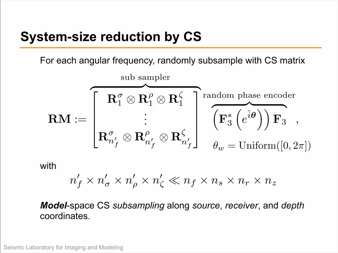
System-size reduction by CSFor each angular frequency, randomly subsample with CS matrix
with
Model-space CS subsampling along source, receiver, and depth coordinates.
RM :=
sub sampler! "# $%
&&'
R!1 !R"
1 !R#1
...R!
n!f!R"
n!f!R#
n!f
(
))*
random phase encoder! "# $+F!
3
+ei!
,,F3 ,
n!f ! n!
! ! n!" ! n!
# " nf ! ns ! nr ! nz
!w = Uniform([0, 2"])
Seismic Laboratory for Imaging and Modeling
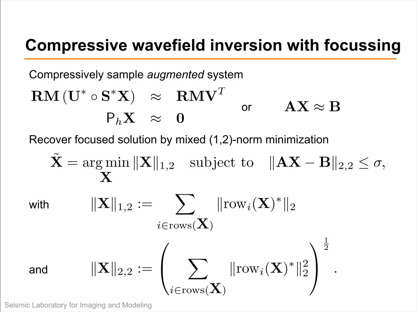
Compressive wavefield inversion with focussingCompressively sample augmented system
or
Recover focused solution by mixed (1,2)-norm minimization
with
and
AX ! BRM (U! ! S!X) " RMVT
PhX " 0
X = arg minX
!X!1,2 subject to !AX"B!2,2 # !,
!X!1,2 :=!
i!rows(X)
!rowi(X)"!2
!X!2,2 :=
!
"#
i!rows(X)
!rowi(X)"!22
$
%
12
.
Seismic Laboratory for Imaging and Modeling
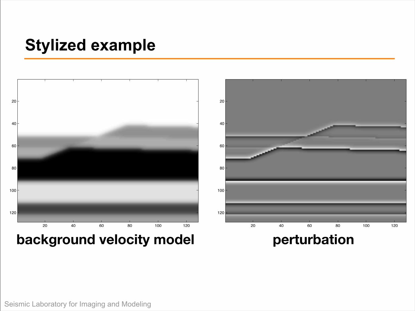
Stylized example
background velocity model perturbation20 40 60 80 100 120
20
40
60
80
100
120
20 40 60 80 100 120
20
40
60
80
100
120
Seismic Laboratory for Imaging and Modeling
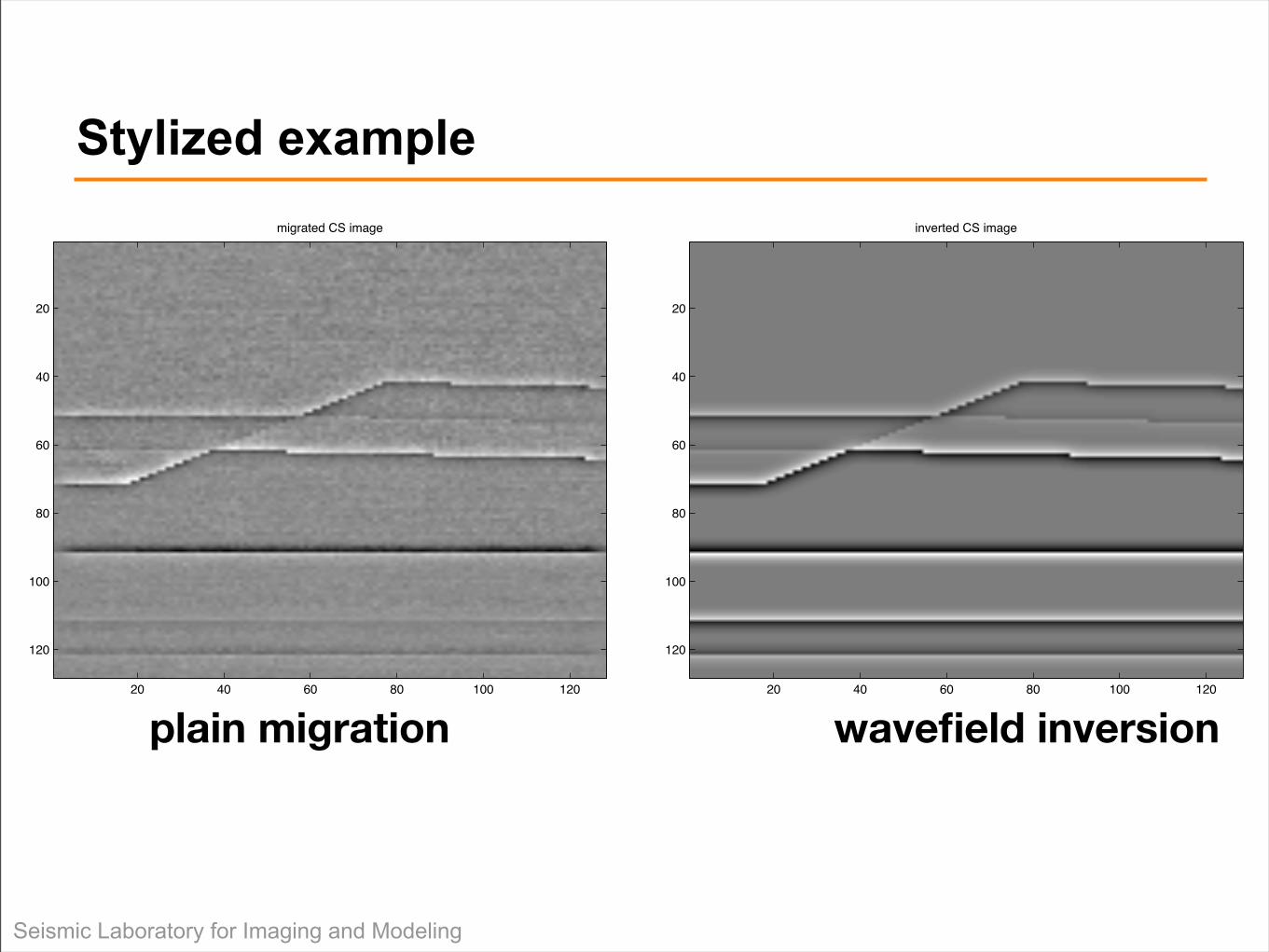
Stylized examplemigrated CS image
20 40 60 80 100 120
20
40
60
80
100
120
inverted CS image
20 40 60 80 100 120
20
40
60
80
100
120
plain migration wavefield inversion
Seismic Laboratory for Imaging and Modeling
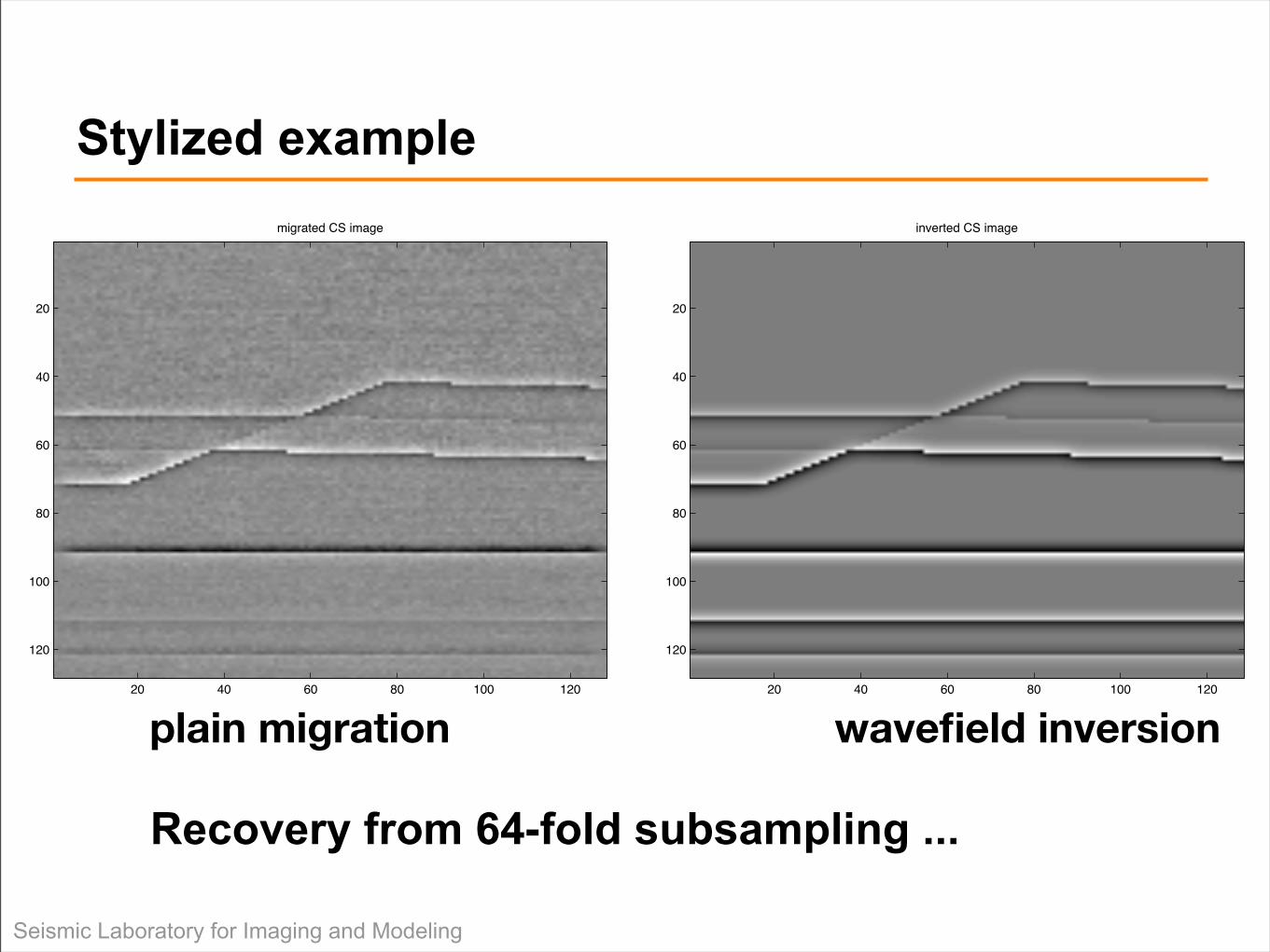
Stylized example
Recovery from 64-fold subsampling ...
migrated CS image
20 40 60 80 100 120
20
40
60
80
100
120
inverted CS image
20 40 60 80 100 120
20
40
60
80
100
120
plain migration wavefield inversion
Seismic Laboratory for Imaging and Modeling
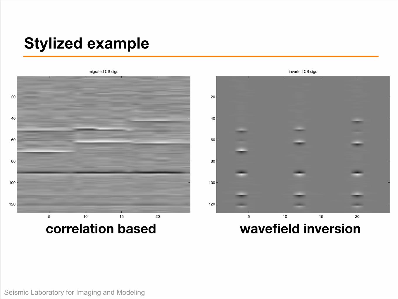
Stylized examplemigrated CS cigs
5 10 15 20
20
40
60
80
100
120
inverted CS cigs
5 10 15 20
20
40
60
80
100
120
correlation based wavefield inversion

Seismic Laboratory for Imaging and Modeling
Stylized examplemigrated CS cigs
5 10 15 20
20
40
60
80
100
120
inverted CS cigs
5 10 15 20
20
40
60
80
100
120
correlation based wavefield inversion
Common-image gathers are focussed.
Seismic Laboratory for Imaging and Modeling
Observations CS provides a new linear sampling paradigm based on randomization
– reduces data volumes and hence acquisition, processing & inversion costs– linearity allows for compressive processing & inversion
CS leads to – “acquisition” of smaller data volumes that carry the same information or– to improved inferences from data using the same resources– concrete implementations
CS combined with physics improved recovery by using– compressively-sampled multiples– focusing in the image space
Bottom line: acquisition & processing & inversion costs are no longer determined by the size of the discretization but by transform-domain sparsity of the solution ...
Seismic Laboratory for Imaging and Modeling
Acknowledgments E. van den Berg and M. P. Friedlander for SPGL1 (www.cs.ubc.ca/
labs/scl/spgl1) & Sparco (www.cs.ubc.ca/labs/scl/sparco) Sergey Fomel and Yang Liu for Madagascar (rsf.sf.net) E. Candes and the Curvelab team
slim.eos.ubc.ca
and... Thank you!
This work was carried out as part of the Collaborative Research & Development (CRD) grant DNOISE (334810-05) funded by the Natural Science and Engineering Research Council (NSERC) and matching contributions from BG, BP, Chevron, ExxonMobil and Shell. FJH would also like to thank the Technische University for their hospitality.