Radon Transform Methods and Their Applicationsin Mapping Mantle Reflectivity Structure

Yu Jeffrey Gu Æ Mauricio Sacchi

Received: 26 October 2008 / Accepted: 1 June 2009� Springer Science+Business Media B.V. 2009

Abstract This paper reviews the fundamentals of Radon-based methods using examples

from global seismic applications. By exploiting the move-out or curvature of signal of

interest, Least-squares and High-resolution Radon transform methods can effectively

eliminate random or correlated noise, enhance signal clarity, and simultaneously constrain

travel time and ray angles. The inverse formulation of the Radon transform has the added

benefits of phase isolation and spatial interpolation during data reconstruction. This study

presents a ‘cookbook’ for Radon-based methods in analyzing shear wave bottom-side

reflections from mantle interfaces, also know as SS precursors. We demonstrate that

accurate and flexible joint Radon- and frequency-domain approaches are particularly

effective in resolving the presence and depth of known and postulated mantle reflectors.

Keywords Radon transform � SS precursor � Seismic discontinuities �Plumes � Hotspot � Mantle structure � Phase transition � Lower mantle reflectors �Subduction zone

1 Introduction

Attenuation of unwanted events such as surface waves and multiples (Yilmaz 1987) poses a

key problem in exploration seismic data processing. Effective solutions to this problem often

exploit the move-out or curvature differences between offending events and the event of

interest. One such solution is the Radon transform, an integral transform (Radon 1917) that

was later adapted not only for the removal of multiple reflections (Thorson and Claerbout

1985; Hampson 1986; Beylkin 1987; Sacchi and Ulrych 1995), but also for wide-ranging

applications in astrophysics (Bracewell 1956), computer tomography (Cormack 1963) and

more recently, regional and global seismology (Gorman and Clowes 1999; Wilson and

Guitton 2007; Ma et al. 2007; An et al. 2007; Gu et al. 2009). Radon transforms in their

discrete form are known for different variations (linear, parabolic, hyperbolic, generalized)

Y. J. Gu (&) � M. SacchiDepartment of Physics, University of Alberta, Edmonton T6G2G7, Canadae-mail: jgu@phys.ualberta.ca

123

Surv GeophysDOI 10.1007/s10712-009-9076-0

and names (slant stack, beam-forming, fan filtration, s-p transform). The method of choice

in a specific application depends on the nature of the source excitation, the inherent prop-

erties of the target signal and, in some cases, computational cost (e.g., Kappus et al. 1990).

For example, parabolic and hyperbolic transforms are the preferred Radon methods if the

data after move-out correction are best characterized by a superposition of parabolas and

hyperbolas, respectively. Inverse formulations have also been developed to enhance the

flexibility and resolution of Radon solutions. In the cases of parabolic (Sacchi and Ulrych

1995) and hyperbolic (Thorson and Claerbout 1985) Radon transforms, the operator capable

of inverting the Radon transform is designed in ways that, when properly executed, the data

in the Radon domain exhibit minimum entropy or maximum sparseness (synonymously used

in this study to describe a distribution of isolated signals in the Radon domain).

The success of Radon-based methods in exploration seismology can potentially be

replicated in global seismic surveys of the crust and mantle reflectivity structure. Apart

from the obvious scale difference between exploration (\20 km) and global (typically

[100 km) problems, key objectives such as signal isolation and enhancement, noise

reduction, and data reconstruction are nearly independent of the applications. Furthermore,

in properly designed global problems, the nominal resolution estimated from the ratio

between wavelength (tens to hundreds of kilometers) and target dimension (often, conti-

nent-scale) could rival the average resolution of exploration imaging. For instance, recent

high-resolution images of the Japan slab (a strong dipping reflector) based on array

analyses of earthquake data (Kawakatsu and Watada 2007; Tonegawa et al. 2008) draw

many parallels to earlier sections of back-scattered head waves (Clayton and McMechan

1981) and present-day reflection profiles of salt domes in oil/gas surveys. Similar success

has been documented at other geographical locations and depths using array methods (see

Rost and Thomas 2002; also see papers in this Special Issue). Coordinated efforts and

substantial resources similar to those put forth by the ongoing USArray project have now

enabled the ‘global community’ to take full advantage of various array methods that

predicate on superior data density and distribution.

In this article we discuss the problem of designing a Radon operator, one of the many

original contributions of exploration seismology, to isolate and filter plane waves reflected

from mantle rocks. The solution entails a transformation that, in the absence of filtering in

the transform domain, is capable of recovering the original data. Our selected case studies

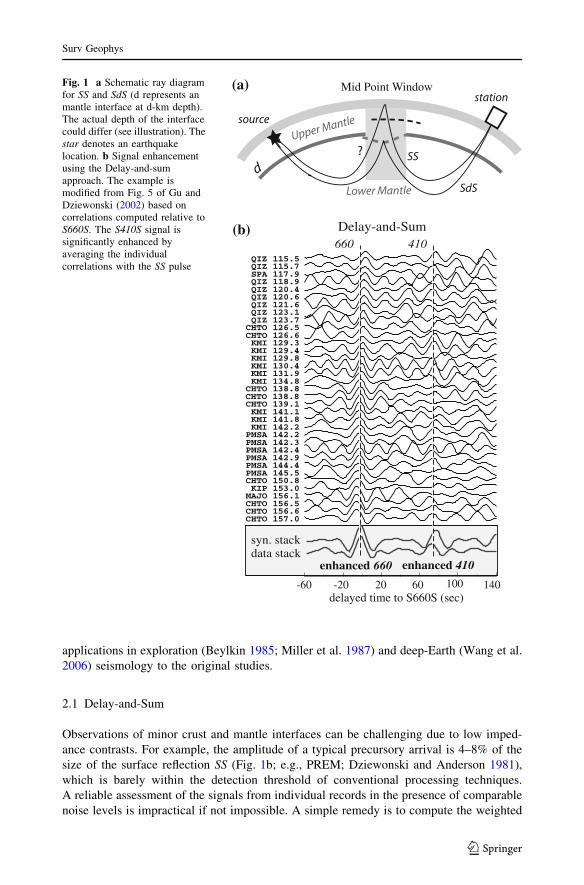
of low-amplitude, underside reflections (or, SS precursors; Fig. 1a) aim to accentuate the

great potential of Radon-based techniques in resolving the large-scale seismic structure,

dynamics and, possibly, mineralogy within the Earth’s mantle.

2 Theory

The section reviews the fundamentals of Radon Transform (RT) methods. While advanced

RT methods have distinct advantages over classical RT approaches, they are based upon

the same elementary operations such as Delay-and-Sum and Slowness Slant Stacking. For

completeness and continuity we summarize the basic formulations and global seismic

applications of each approach. We mainly emphasize the role of Radon transform as a

signal identification and enhancement tool, a view often shared in exploration seismic

applications. It should be recognized, however, that Radon transforms can be generalized

to solve the linear Born scattering problem with asymptotic Green functions. We defer the

discussion of Generalized Radon Transform (GRT) method and its contributions to

Surv Geophys

123

applications in exploration (Beylkin 1985; Miller et al. 1987) and deep-Earth (Wang et al.

2006) seismology to the original studies.

2.1 Delay-and-Sum

Observations of minor crust and mantle interfaces can be challenging due to low imped-

ance contrasts. For example, the amplitude of a typical precursory arrival is 4–8% of the

size of the surface reflection SS (Fig. 1b; e.g., PREM; Dziewonski and Anderson 1981),

which is barely within the detection threshold of conventional processing techniques.

A reliable assessment of the signals from individual records in the presence of comparable

noise levels is impractical if not impossible. A simple remedy is to compute the weighted

?

source

station

dSdS

Upper Mantle

(a)

CHTO 157.0 CHTO 156.6 CHTO 156.5 MAJO 156.1 KIP 153.0 CHTO 150.8 PMSA 145.5 PMSA 144.4 PMSA 142.9 PMSA 142.4 PMSA 142.3 PMSA 142.2 KMI 142.2 KMI 141.8 KMI 141.1 CHTO 139.1 CHTO 138.8 CHTO 138.8 KMI 134.8 KMI 131.9 KMI 130.4 KMI 129.8 KMI 129.4 KMI 129.3 CHTO 126.6 CHTO 126.5 QIZ 123.7 QIZ 123.1 QIZ 121.6 QIZ 120.6 QIZ 120.4 QIZ 118.9 SPA 117.9 QIZ 115.7 QIZ 115.5

Delay-and-Sum

syn. stackdata stack

410660

delayed time to S660S (sec)-60 -20 20 60 100 140

enhanced 410enhanced 660

(b)

Lower Mantle

SS

Mid Point WindowFig. 1 a Schematic ray diagramfor SS and SdS (d represents anmantle interface at d-km depth).The actual depth of the interfacecould differ (see illustration). Thestar denotes an earthquakelocation. b Signal enhancementusing the Delay-and-sumapproach. The example ismodified from Fig. 5 of Gu andDziewonski (2002) based oncorrelations computed relative toS660S. The S410S signal issignificantly enhanced byaveraging the individualcorrelations with the SS pulse

Surv Geophys

123

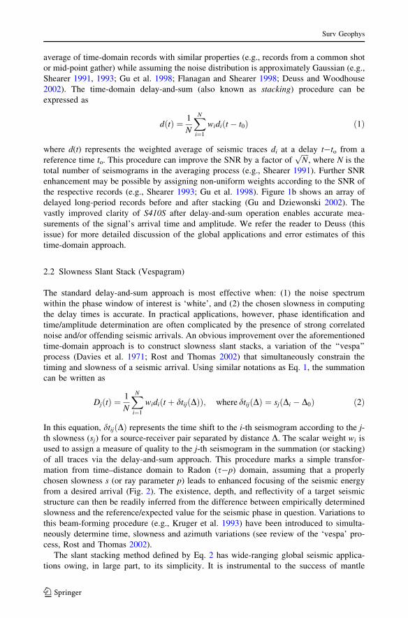
average of time-domain records with similar properties (e.g., records from a common shot

or mid-point gather) while assuming the noise distribution is approximately Gaussian (e.g.,

Shearer 1991, 1993; Gu et al. 1998; Flanagan and Shearer 1998; Deuss and Woodhouse

2002). The time-domain delay-and-sum (also known as stacking) procedure can be

expressed as

dðtÞ ¼ 1

N

XN

i¼1

widiðt � t0Þ ð1Þ

where d(t) represents the weighted average of seismic traces di at a delay t-to from a

reference time to. This procedure can improve the SNR by a factor offfiffiffiffiNp

, where N is the

total number of seismograms in the averaging process (e.g., Shearer 1991). Further SNR

enhancement may be possible by assigning non-uniform weights according to the SNR of

the respective records (e.g., Shearer 1993; Gu et al. 1998). Figure 1b shows an array of

delayed long-period records before and after stacking (Gu and Dziewonski 2002). The

vastly improved clarity of S410S after delay-and-sum operation enables accurate mea-

surements of the signal’s arrival time and amplitude. We refer the reader to Deuss (this

issue) for more detailed discussion of the global applications and error estimates of this

time-domain approach.

2.2 Slowness Slant Stack (Vespagram)

The standard delay-and-sum approach is most effective when: (1) the noise spectrum

within the phase window of interest is ‘white’, and (2) the chosen slowness in computing

the delay times is accurate. In practical applications, however, phase identification and

time/amplitude determination are often complicated by the presence of strong correlated

noise and/or offending seismic arrivals. An obvious improvement over the aforementioned

time-domain approach is to construct slowness slant stacks, a variation of the ‘‘vespa’’

process (Davies et al. 1971; Rost and Thomas 2002) that simultaneously constrain the

timing and slowness of a seismic arrival. Using similar notations as Eq. 1, the summation

can be written as

DjðtÞ ¼1

N

XN

i¼1

widiðt þ dtijðDÞÞ; where dtijðDÞ ¼ sjðDi � D0Þ ð2Þ

In this equation, dtijðDÞ represents the time shift to the i-th seismogram according to the j-th slowness (sj) for a source-receiver pair separated by distance D. The scalar weight wi is

used to assign a measure of quality to the j-th seismogram in the summation (or stacking)

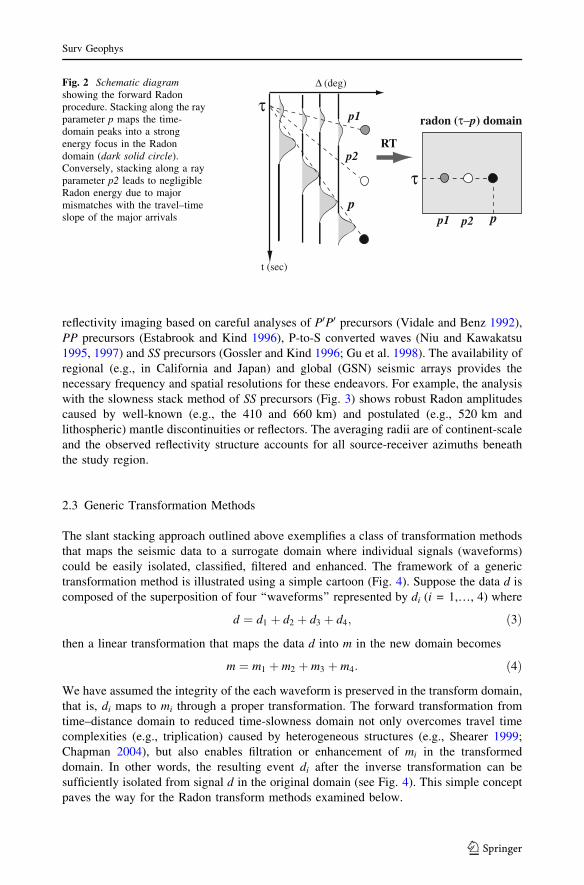
of all traces via the delay-and-sum approach. This procedure marks a simple transfor-

mation from time–distance domain to Radon (s-p) domain, assuming that a properly

chosen slowness s (or ray parameter p) leads to enhanced focusing of the seismic energy

from a desired arrival (Fig. 2). The existence, depth, and reflectivity of a target seismic

structure can then be readily inferred from the difference between empirically determined

slowness and the reference/expected value for the seismic phase in question. Variations to

this beam-forming procedure (e.g., Kruger et al. 1993) have been introduced to simulta-

neously determine time, slowness and azimuth variations (see review of the ‘vespa’ pro-

cess, Rost and Thomas 2002).

The slant stacking method defined by Eq. 2 has wide-ranging global seismic applica-

tions owing, in large part, to its simplicity. It is instrumental to the success of mantle

Surv Geophys

123

reflectivity imaging based on careful analyses of P0P0 precursors (Vidale and Benz 1992),

PP precursors (Estabrook and Kind 1996), P-to-S converted waves (Niu and Kawakatsu

1995, 1997) and SS precursors (Gossler and Kind 1996; Gu et al. 1998). The availability of

regional (e.g., in California and Japan) and global (GSN) seismic arrays provides the

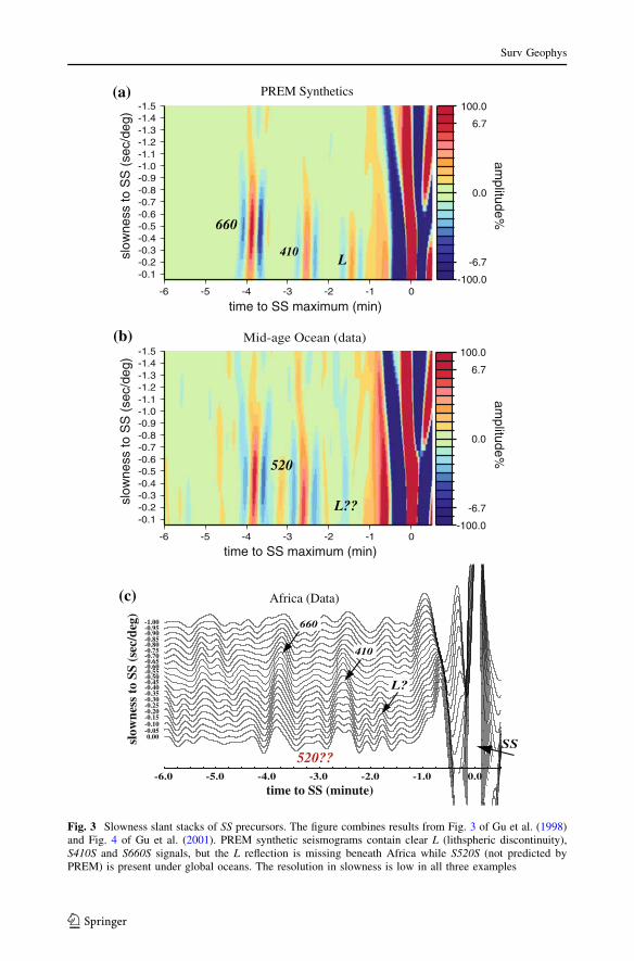
necessary frequency and spatial resolutions for these endeavors. For example, the analysis

with the slowness stack method of SS precursors (Fig. 3) shows robust Radon amplitudes

caused by well-known (e.g., the 410 and 660 km) and postulated (e.g., 520 km and

lithospheric) mantle discontinuities or reflectors. The averaging radii are of continent-scale

and the observed reflectivity structure accounts for all source-receiver azimuths beneath

the study region.

2.3 Generic Transformation Methods

The slant stacking approach outlined above exemplifies a class of transformation methods

that maps the seismic data to a surrogate domain where individual signals (waveforms)

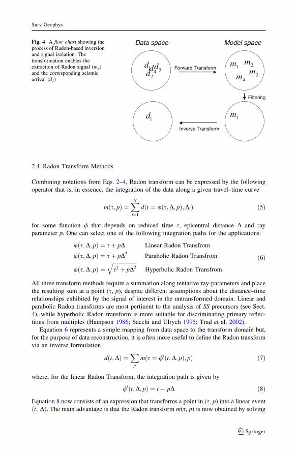
could be easily isolated, classified, filtered and enhanced. The framework of a generic

transformation method is illustrated using a simple cartoon (Fig. 4). Suppose the data d is

composed of the superposition of four ‘‘waveforms’’ represented by di (i = 1,…, 4) where

d ¼ d1 þ d2 þ d3 þ d4; ð3Þ

then a linear transformation that maps the data d into m in the new domain becomes

m ¼ m1 þ m2 þ m3 þ m4: ð4Þ

We have assumed the integrity of the each waveform is preserved in the transform domain,

that is, di maps to mi through a proper transformation. The forward transformation from

time–distance domain to reduced time-slowness domain not only overcomes travel time

complexities (e.g., triplication) caused by heterogeneous structures (e.g., Shearer 1999;

Chapman 2004), but also enables filtration or enhancement of mi in the transformed

domain. In other words, the resulting event di after the inverse transformation can be

sufficiently isolated from signal d in the original domain (see Fig. 4). This simple concept

paves the way for the Radon transform methods examined below.

RT

radon (τ−p) domain

p1 p2 p

τ

τ

t (sec)

∆ (deg)

p

p1

p2

Fig. 2 Schematic diagramshowing the forward Radonprocedure. Stacking along the rayparameter p maps the time-domain peaks into a strongenergy focus in the Radondomain (dark solid circle).Conversely, stacking along a rayparameter p2 leads to negligibleRadon energy due to majormismatches with the travel–timeslope of the major arrivals

Surv Geophys

123

-6.0 -5.0 -4.0 -3.0 -2.0 -1.0 0.0

time to SS (minute)

0.00 -0.05 -0.10 -0.15 -0.20 -0.25 -0.30 -0.35 -0.40 -0.45 -0.50 -0.55 -0.60 -0.65 -0.70 -0.75 -0.80 -0.85 -0.90 -0.95 -1.00

slow

ness

to

SS (

sec/

deg)

L?

660

410

SS

(c) Africa (Data)

520??

-1.5 -1.4 -1.3 -1.2 -1.1 -1.0 -0.9 -0.8 -0.7 -0.6 -0.5 -0.4 -0.3 -0.2 -0.1

slo

wne

ss to

SS

(se

c/de

g)

-6 -5 -4 -3 -2 -1 0

Mid-age Ocean (data) -1.5 -1.4 -1.3 -1.2 -1.1 -1.0 -0.9 -0.8 -0.7 -0.6 -0.5 -0.4 -0.3 -0.2 -0.1

slo

wne

ss to

SS

(se

c/de

g)

-6 -5 -4 -3 -2 -1 0

time to SS maximum (min)

PREM Synthetics

time to SS maximum (min)

-100.0

-6.7

0.0

6.7

100.0

-100.0

-6.7

0.0

6.7

100.0

amplitude%

am

plitude%

(a)

(b)

660

410L

520

L??

Fig. 3 Slowness slant stacks of SS precursors. The figure combines results from Fig. 3 of Gu et al. (1998)and Fig. 4 of Gu et al. (2001). PREM synthetic seismograms contain clear L (lithspheric discontinuity),S410S and S660S signals, but the L reflection is missing beneath Africa while S520S (not predicted byPREM) is present under global oceans. The resolution in slowness is low in all three examples

Surv Geophys

123

2.4 Radon Transform Methods

Combining notations from Eqs. 2–4, Radon transform can be expressed by the following

operator that is, in essence, the integration of the data along a given travel–time curve

mðs; pÞ ¼XN

i¼1

dðt ¼ /ðs;D; pÞ;DiÞ ð5Þ

for some function / that depends on reduced time s, epicentral distance D and ray

parameter p. One can select one of the following integration paths for the applications:

/ðs;D; pÞ ¼ sþ pD Linear Radon Transfrom

/ðs;D; pÞ ¼ sþ pD2 Parabolic Radon Transfrom

/ðs;D; pÞ ¼ffiffiffiffiffiffiffiffiffiffiffiffiffiffiffiffiffiffis2 þ pD2

qHyperbolic Radon Transfrom:

ð6Þ

All three transform methods require a summation along tentative ray-parameters and place

the resulting sum at a point (s, p), despite different assumptions about the distance–time

relationships exhibited by the signal of interest in the untransformed domain. Linear and

parabolic Radon transforms are most pertinent to the analysis of SS precursors (see Sect.

4), while hyperbolic Radon transform is more suitable for discriminating primary reflec-

tions from multiples (Hampson 1986; Sacchi and Ulrych 1995; Trad et al. 2002).

Equation 6 represents a simple mapping from data space to the transform domain but,

for the purpose of data reconstruction, it is often more useful to define the Radon transform

via an inverse formulation

dðt;DÞ ¼X

p

mðs ¼ /0ðt;D; pÞ; pÞ ð7Þ

where, for the linear Radon Transform, the integration path is given by

/0ðt;D; pÞ ¼ t � pD ð8Þ

Equation 8 now consists of an expression that transforms a point in (s, p) into a linear event

ðt; DÞ. The main advantage is that the Radon transform m(s, p) is now obtained by solving

Data space Model space

Forward Transform

Inverse Transform

d1d4d2

d3m1

m3m4

m2

m1d1

Filtering

Fig. 4 A flow chart showing theprocess of Radon-based inversionand signal isolation. Thetransformation enables theextraction of Radon signal (m1)and the corresponding seismicarrival (d1)

Surv Geophys

123

a linear inverse problem of the form d=Am, where A is the sensitivity matrix and the d is

the data vector.

2.5 Inversion of Radon Transform

Details pertaining to the synthesis of Eq. 8 were provided by Thorson and Claerbout (1985)

and Hampson (1986). In this review we mainly focus on a frequency-domain solution

adopted by An et al. (2007). By Fourier transform both sides of Eq. 8 and subsequently

apply the Fourier delay theorem (Papoulis 1962), we obtain the following expression for

each angular frequency x:

Dðx;DkÞ ¼XNP

j¼1

Mðx; pjÞe�ixDkpj ; k ¼ 1; . . .;N ð9Þ

where N is the total number of time series in the data gather, x is a single angular

frequency and NP denotes the total number of ray parameters within the desired s-prange. Capitalized letters D and M represent the Fourier transform of d and m (see Eq. 7),

respectively. Equation 9 represents a matrix equation of the form

Dðx;D1ÞDðx;D2Þ

:

:

:Dðx;DNÞ

0BBBBBBB@

1CCCCCCCA

¼

e�ixD1p1 e�ixD1p2 : e�ixD1pM

e�ixD2p1 e�ixD2p2 : e�ixD2pM

:

:

:

:

:

:

:

:

:

:

:

:

e�ixDN p1 e�ixDN p2 : e�ixDN pM

0BBBBBBB@

1CCCCCCCA

Mðx; p1ÞMðx; p2Þ

:

:Mðx; pNPÞ

0BBBB@

1CCCCA

ð10Þ

or simply,

DðxÞ ¼ AðxÞMðxÞ ð11Þ

The vector MðxÞ represents Radon solution for a monochromatic frequency component xin a linear inverse problem. Equation 11 is usually solved using the damped least-squares

method (Menke 1989; Parker 1994) that minimizes the following cost function:

J ¼ jjDðxÞ � AðxÞMðxÞjj22 þ l jjMðxÞjj22 ð12Þ

The first two terms on the right-hand side represent the data misfit, a measure of the

predictive error of the forward Radon operator. The second term is a regularization (also

known as damping or penalty) term to stabilize the solution. We have also introduced a

trade-off parameter l to control the fidelity to which the forward Radon operator can fit the

data. The final solution is determined via minimizing Eq. 12 with respect to the unknown

solution vector MðxÞ. Once MðxÞ is determined for all angular frequencies x, we can

recover the Radon operator mðs; pjÞ in the time domain via inverse Fourier transform and

insert the outcome into Eq. 9 for time-domain data reconstruction and interpolation. We

refer to the above procedure as the damped Least-Squares Radon Transform (LSRT).

The choice of objective function in Eq. 12 is not unique. Alternatives such as non-

quadratic regularization methods have been previously adopted (Sacchi and Ulrych 1995;

Wilson and Guitton 2007) to increase the resolution of Radon images. For example, the

regularization term can be chosen as Cauchy or L1 norm to enhance the resolution of the

transform (Sacchi and Ulrych 1995). Methods based on these regularization/reweighting

strategies have been referred to as High-resolution Radon Transforms (HRT). The remainder

Surv Geophys

123

of this review considers applications using both LSRT (for northeastern Pacific and western

Canada) and HRT (for mapping global hotspots) methods.

3 SS Precursors and Preliminary Radon Analysis

3.1 Data Preparation and Problem Setup

The main data set reviewed below consists of broadband and long-period recordings from

Global Seismic Network (GSN), GEOSCOPE and several regional seismic networks. We

select records from shallow events (\45 km) to minimize the interference from depth phases

(e.g., sSS); a higher cutoff value of 75 km has been adopted by global time-domain analyses

(e.g., Shearer 1993; Flanagan and Shearer 1998) to improve data density at the expense of

reduced data quality. We further restrict the magnitude (Mw) to[5 and epicentral distance to

100–160 deg; the latter requirement minimizes waveform interference from topside

reflection sdsS and ScS precursors ScSdScS, where d denotes the depth of the corresponding

reflection surface as in Fig. 1a (Schmerr and Garnero 2006). The transverse component

seismograms are then filtered between 0.0013 and 0.08 Hz and subjected to a SNR (defined

by the ratio between SS and its proceeding ‘noise’ level) test; all records with SNR lower

than 3.0 are automatically rejected. We improve the data quality further by interactively

inspecting all seismograms using a MATLAB-based visualization code and reverse the

polarity of problematic station records to account for potential instrument misorientation.

We partition the data using circular, 5–10 deg (roughly equivalent to 500–1,000 km)

radius spherical gathers (or ‘‘caps’’, Shearer 1991) of SS reflection points (also see Deuss,

this issue). The sizes of the caps vary in order to maintain sufficient data density. The

combination of natural frequency (15–20 s) and averaging radii is mainly responsible for

the effective Fresnel zone of *1,500 km (Shearer 1993; Rost and Thomas, this issue).

These mid-point gathers may partially overlap and introduce further spatial averaging

within the region of interest.

3.2 Data Pre-Conditioning

In theory, LSRT/HRT can be directly applied to the reflections and conversions from

mantle discontinuities. In practice, however, the recorded SS precursors often require

additional signal enhancement due to correlated/random noise and incomplete data cov-

erage. Without pre-conditioning LSRT/HRT cannot effectively collapse the time domain

reflections to discrete s-p values as seen in Fig. 2 since the scatter in the Radon domain

can be as severe as it is in time domain (An et al. 2007). The solution is to pre-condition the

time series by computing the running averages of SS precursors along some theoretical

move-out curves. The size of the running-average (or, partial stacking) window trades off

with resolution. The nominal resolution using empirical window lengths of 20–30 deg (An

et al. 2007; Gu et al. 2009) is 40–50% higher than those achievable by time-domain

approaches (averaged over 60–70 deg typically) within the same gather (e.g., Shearer

1993; Flanagan and Shearer 1998; Gu et al. 2003; Deuss and Woodhouse 2001; Tauzin

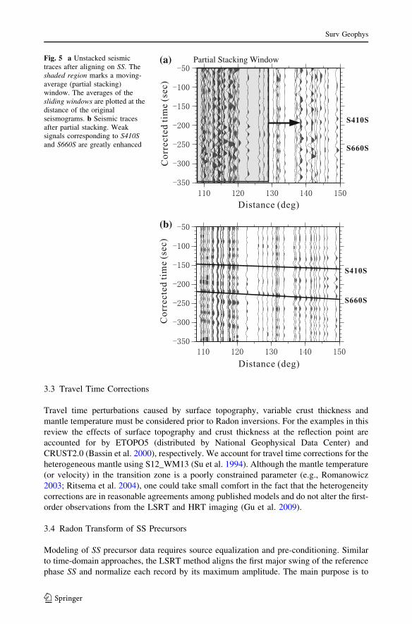
et al. 2008). While the original time series (Fig. 5a) leads to incoherent signals in Radon

space, the partially stacked series (Fig. 5b) both preserves the coherent move-outs and

produces measureable Radon peaks. The superior resolution of HRT enables an effective

separation of the maximum and minimum energy peaks for each seismic arrival (see

Fig. 5b); only the maxima are used in the calculation of reflection depths.

Surv Geophys

123

3.3 Travel Time Corrections

Travel time perturbations caused by surface topography, variable crust thickness and

mantle temperature must be considered prior to Radon inversions. For the examples in this

review the effects of surface topography and crust thickness at the reflection point are

accounted for by ETOPO5 (distributed by National Geophysical Data Center) and

CRUST2.0 (Bassin et al. 2000), respectively. We account for travel time corrections for the

heterogeneous mantle using S12_WM13 (Su et al. 1994). Although the mantle temperature

(or velocity) in the transition zone is a poorly constrained parameter (e.g., Romanowicz

2003; Ritsema et al. 2004), one could take small comfort in the fact that the heterogeneity

corrections are in reasonable agreements among published models and do not alter the first-

order observations from the LSRT and HRT imaging (Gu et al. 2009).

3.4 Radon Transform of SS Precursors

Modeling of SS precursor data requires source equalization and pre-conditioning. Similar

to time-domain approaches, the LSRT method aligns the first major swing of the reference

phase SS and normalize each record by its maximum amplitude. The main purpose is to

Partial Stacking Window(a)

(b)

Fig. 5 a Unstacked seismictraces after aligning on SS. Theshaded region marks a moving-average (partial stacking)window. The averages of thesliding windows are plotted at thedistance of the originalseismograms. b Seismic tracesafter partial stacking. Weaksignals corresponding to S410Sand S660S are greatly enhanced

Surv Geophys

123

equalize the source, as the SS-SdS relative times are less affected by origin time uncertainty

or source complexity. For consistency the ray parameter p of a given signal of interest (e.g.,

S660S) is expressed as the differential ray parameters to SS; p is approximately constant for

the appropriate distance range (An et al. 2007; Gu et al. 2009). The process of aligning SSis equivalent to setting the reference ray parameter to a value of zero. Unlike time-domain

analyses (see review by Deuss, this issue), Radon-based methods preserve the relative

move-out between SS and SdS.

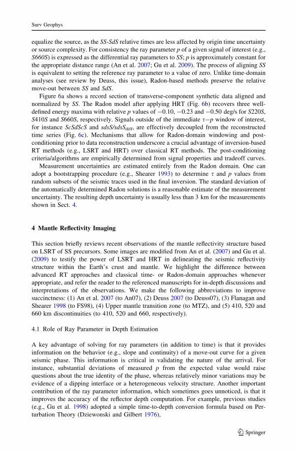
Figure 6a shows a record section of transverse-component synthetic data aligned and

normalized by SS. The Radon model after applying HRT (Fig. 6b) recovers three well-

defined energy maxima with relative p values of -0.10, -0.23 and -0.50 deg/s for S220S,

S410S and S660S, respectively. Signals outside of the immediate s-p window of interest,

for instance ScSdScS and sdsS/sdsSdiff, are effectively decoupled from the reconstructed

time series (Fig. 6c). Mechanisms that allow for Radon-domain windowing and post-

conditioning prior to data reconstruction underscore a crucial advantage of inversion-based

RT methods (e.g., LSRT and HRT) over classical RT methods. The post-conditioning

criteria/algorithms are empirically determined from signal properties and tradeoff curves.

Measurement uncertainties are estimated entirely from the Radon domain. One can

adopt a bootstrapping procedure (e.g., Shearer 1993) to determine s and p values from

random subsets of the seismic traces used in the final inversion. The standard deviation of

the automatically determined Radon solutions is a reasonable estimate of the measurement

uncertainty. The resulting depth uncertainty is usually less than 3 km for the measurements

shown in Sect. 4.

4 Mantle Reflectivity Imaging

This section briefly reviews recent observations of the mantle reflectivity structure based

on LSRT of SS precursors. Some images are modified from An et al. (2007) and Gu et al.

(2009) to testify the power of LSRT and HRT in delineating the seismic reflectivity

structure within the Earth’s crust and mantle. We highlight the difference between

advanced RT approaches and classical time- or Radon-domain approaches whenever

appropriate, and refer the reader to the referenced manuscripts for in-depth discussions and

interpretations of the observations. We make the following abbreviations to improve

succinctness: (1) An et al. 2007 (to An07), (2) Deuss 2007 (to Deuss07), (3) Flanagan and

Shearer 1998 (to FS98), (4) Upper mantle transition zone (to MTZ), and (5) 410, 520 and

660 km discontinuities (to 410, 520 and 660, respectively).

4.1 Role of Ray Parameter in Depth Estimation

A key advantage of solving for ray parameters (in addition to time) is that it provides

information on the behavior (e.g., slope and continuity) of a move-out curve for a given

seismic phase. This information is critical in validating the nature of the arrival. For

instance, substantial deviations of measured p from the expected value would raise

questions about the true identity of the phase, whereas relatively minor variations may be

evidence of a dipping interface or a heterogeneous velocity structure. Another important

contribution of the ray parameter information, which sometimes goes unnoticed, is that it

improves the accuracy of the reflector depth computation. For example, previous studies

(e.g., Gu et al. 1998) adopted a simple time-to-depth conversion formula based on Per-

turbation Theory (Dziewonski and Gilbert 1976),

Surv Geophys

123

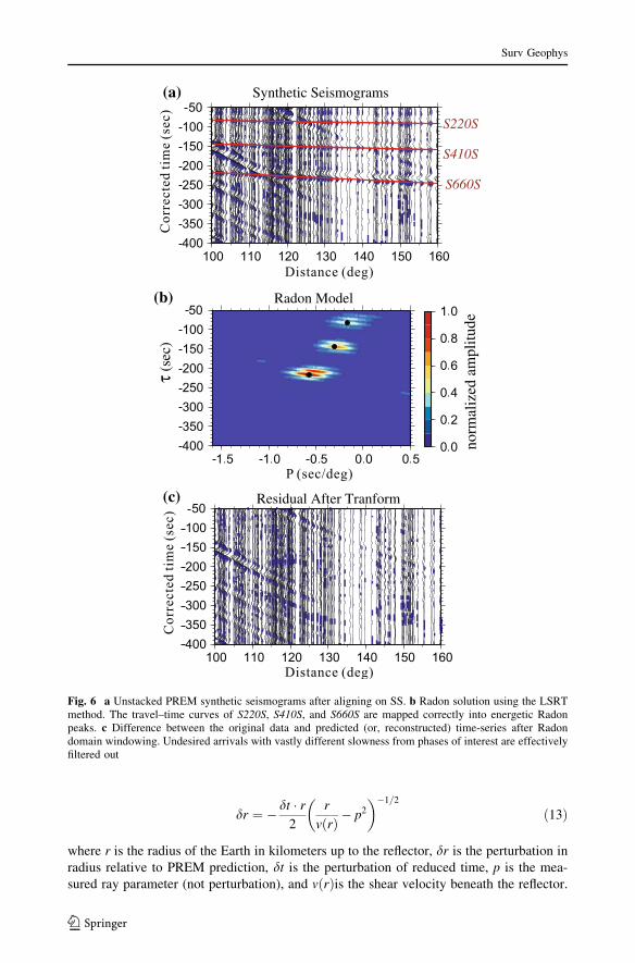
dr ¼ � dt � r2

r

vðrÞ � p2

� ��1=2

ð13Þ

where r is the radius of the Earth in kilometers up to the reflector, dr is the perturbation in

radius relative to PREM prediction, dt is the perturbation of reduced time, p is the mea-

sured ray parameter (not perturbation), and vðrÞis the shear velocity beneath the reflector.

S220S

S660S

S410S

edutil pma

dezil amr on

Radon Model (b)

(a)

(c) Residual After Tranform

Synthetic Seismograms

τ(s

ec)

Fig. 6 a Unstacked PREM synthetic seismograms after aligning on SS. b Radon solution using the LSRTmethod. The travel–time curves of S220S, S410S, and S660S are mapped correctly into energetic Radonpeaks. c Difference between the original data and predicted (or, reconstructed) time-series after Radondomain windowing. Undesired arrivals with vastly different slowness from phases of interest are effectivelyfiltered out

Surv Geophys

123

The negative sign implies that a depressed boundary (negative dr) will cause a time delay

(positive dt). This formula, as well as other approaches such as travel time ray tracing (e.g.,

Gossler and Kind 1996), require ray angle information to produce accurate reflector depths.

However, most time-domain approaches relied on theoretical (constant) ray parameters

from a reference Earth model and are, by default, less accurate than Radon-based methods

(including slowness slant stacks) where dipping and heterogeneous structures are properly

accounted for by the measured ray parameters.

4.2 Vespa versus LSRT

A crucial difference between slowness slant stack and inversion-based Radon methods is

the latter’s ability to reconstruct and interpolate time-domain data. For instance, the Radon

solution and resulting misfit to the original time series can be readily adjusted through a

regularization (damping) parameter (see Eq. 12). Once the desired Radon solution is

obtained, one can interpolate over gaps in receiver coverage by increasing the spatial

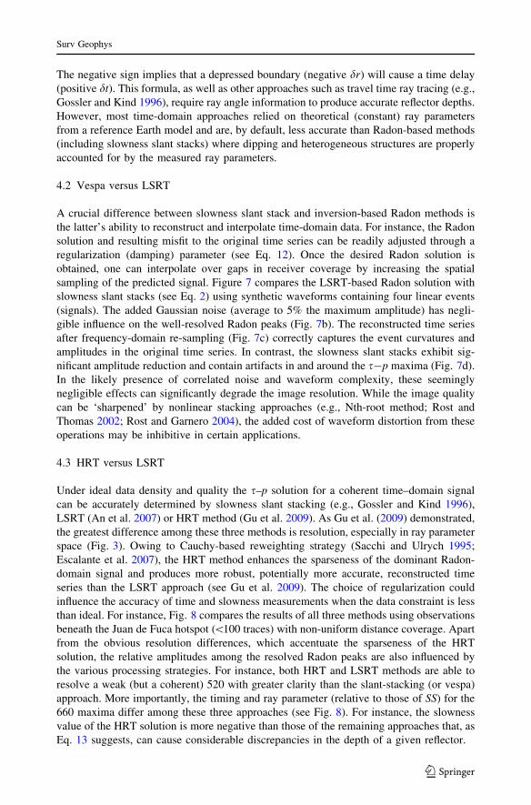
sampling of the predicted signal. Figure 7 compares the LSRT-based Radon solution with

slowness slant stacks (see Eq. 2) using synthetic waveforms containing four linear events

(signals). The added Gaussian noise (average to 5% the maximum amplitude) has negli-

gible influence on the well-resolved Radon peaks (Fig. 7b). The reconstructed time series

after frequency-domain re-sampling (Fig. 7c) correctly captures the event curvatures and

amplitudes in the original time series. In contrast, the slowness slant stacks exhibit sig-

nificant amplitude reduction and contain artifacts in and around the s-p maxima (Fig. 7d).

In the likely presence of correlated noise and waveform complexity, these seemingly

negligible effects can significantly degrade the image resolution. While the image quality

can be ‘sharpened’ by nonlinear stacking approaches (e.g., Nth-root method; Rost and

Thomas 2002; Rost and Garnero 2004), the added cost of waveform distortion from these

operations may be inhibitive in certain applications.

4.3 HRT versus LSRT

Under ideal data density and quality the s–p solution for a coherent time–domain signal

can be accurately determined by slowness slant stacking (e.g., Gossler and Kind 1996),

LSRT (An et al. 2007) or HRT method (Gu et al. 2009). As Gu et al. (2009) demonstrated,

the greatest difference among these three methods is resolution, especially in ray parameter

space (Fig. 3). Owing to Cauchy-based reweighting strategy (Sacchi and Ulrych 1995;

Escalante et al. 2007), the HRT method enhances the sparseness of the dominant Radon-

domain signal and produces more robust, potentially more accurate, reconstructed time

series than the LSRT approach (see Gu et al. 2009). The choice of regularization could

influence the accuracy of time and slowness measurements when the data constraint is less

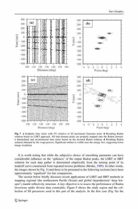
than ideal. For instance, Fig. 8 compares the results of all three methods using observations

beneath the Juan de Fuca hotspot (\100 traces) with non-uniform distance coverage. Apart

from the obvious resolution differences, which accentuate the sparseness of the HRT

solution, the relative amplitudes among the resolved Radon peaks are also influenced by

the various processing strategies. For instance, both HRT and LSRT methods are able to

resolve a weak (but a coherent) 520 with greater clarity than the slant-stacking (or vespa)

approach. More importantly, the timing and ray parameter (relative to those of SS) for the

660 maxima differ among these three approaches (see Fig. 8). For instance, the slowness

value of the HRT solution is more negative than those of the remaining approaches that, as

Eq. 13 suggests, can cause considerable discrepancies in the depth of a given reflector.

Surv Geophys

123

It is worth noting that while the subjective choice of smoothing parameter can have

considerable influence on the ‘spikiness’ of the output Radon peaks, the LSRT or HRT

solution for each data gather is determined empirically from the turning point of its

tradeoff curve constructed from repeated inverse problems (Menke, 1989). In other words,

the images shown by Fig. 8 (and those to be presented in the following sections) have been

approximately ‘equalized’ for fair comparisons.

The section below briefly discusses recent applications of LSRT and HRT methods in

mapping regional (the northeastern Pacific Ocean) and global (hypothesized ‘deep hot-

spot’) mantle reflectivity structure. A key objective is to assess the performance of Radon

inversions under diverse data constraints. Figure 9 shows the study region and the col-

lection of SS precursors used in this part of the analysis. In the first case (Fig. 9a) the

(a) (b)

(c) (d)

Fig. 7 a Synthetic time series with 5% (relative to SS maximum) Gaussian noise. b Resulting Radonsolution based on LSRT approach. All time-domain peaks are properly mapped onto the Radon domain.c Interpolated and reconstructed time series based on the inverted Radon solution. d Resulting Radonsolution obtained by the vespa process. Significant artifact is visible near the energy foci, suggesting lowerimage resolution

Surv Geophys

123

density of mid-point reflections increases toward the northeast, prompting the use of

variable partial-averaging windows (30 deg for the first two gathers and 20 deg for the

remaining gathers) for data pre-conditioning. The global survey of hotspots utilizes a

uniform cap radius of 10 deg as well as variable distance windows determined by the SNR.

We restrict the distance range to 125–160 deg (instead of 100–160 deg) for some hotspots

(e.g., Reunion, Hawaii among others) to remove a slowness discontinuity at a distances of

*120 deg. Hotspots within the Pacific Ocean generally have greater data coverage than

others.

4.4 LSRT-Based Reflectivity Imaging Beneath Northeastern Pacific Ocean

and Western Canada

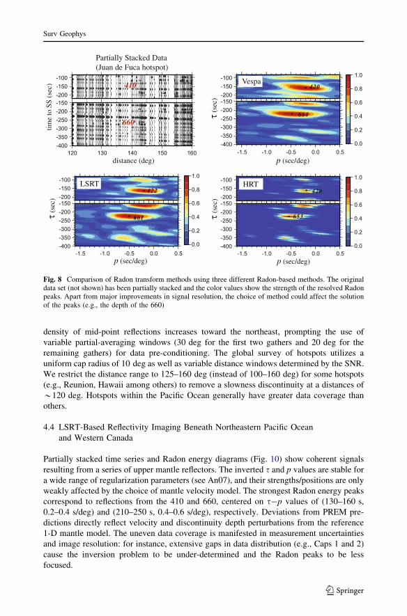
Partially stacked time series and Radon energy diagrams (Fig. 10) show coherent signals

resulting from a series of upper mantle reflectors. The inverted s and p values are stable for

a wide range of regularization parameters (see An07), and their strengths/positions are only

weakly affected by the choice of mantle velocity model. The strongest Radon energy peaks

correspond to reflections from the 410 and 660, centered on s-p values of (130–160 s,

0.2–0.4 s/deg) and (210–250 s, 0.4–0.6 s/deg), respectively. Deviations from PREM pre-

dictions directly reflect velocity and discontinuity depth perturbations from the reference

1-D mantle model. The uneven data coverage is manifested in measurement uncertainties

and image resolution: for instance, extensive gaps in data distribution (e.g., Caps 1 and 2)

cause the inversion problem to be under-determined and the Radon peaks to be less

focused.

Partially Stacked Data (Juan de Fuca hotspot)

distance (deg)

)ces( SS ot emit

p (sec/deg)

p (sec/deg)

p (sec/deg)

Vespa

LSRT HRT

τ)ces(

410

660

τ)ces(

τ (s

ec)

Fig. 8 Comparison of Radon transform methods using three different Radon-based methods. The originaldata set (not shown) has been partially stacked and the color values show the strength of the resolved Radonpeaks. Apart from major improvements in signal resolution, the choice of method could affect the solutionof the peaks (e.g., the depth of the 660)

Surv Geophys

123

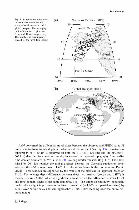
An07 converted the differential travel times between the observed and PREM-based SSprecursors to discontinuity depth perturbations at the intercept (see Eq. 13). Peak-to-peak

topography of *30 km is observed on both the 410 (391–420 km) and the 660 (634–

667 km) that, despite consistent trends, far exceed the reported topography from earlier

time-domain estimates (FS98; Gu et al. 2003) along similar transects (Fig. 11a). The 410 is

raised by 20? km relative the global average beneath the Cascadia subduction zone,

whereas the 660 shows broad, 15–20 km elevations beneath the northeastern Pacific

Ocean. These features are supported by the results of the classical RT approach based on

Eq. 2. The average depth difference between these two methods (vespa and LSRT) is

merely *3 km (An07), which is significantly smaller than the difference between LSRT

and time-domain stacks of the same data (Fig. 11b). The larger discontinuity topography

could reflect slight improvements in lateral resolution (*1,000 km; partial stacking) by

LSRT over earlier delay-and-sum approaches (1,500? km; stacking over the entire dis-

tance range).

Iceland

CAN

CAPENEAZ

Global Hotspots (HRT)

YE

Afar

ReunionTahiti Pitcarin

LouisvilleMacdonald

Samoa Marqueses

Hawaii

BowieJDF

(b)

Northeast Pacific (LSRT)

160W180W 120W 100W140W

(a)Fig. 9 SS reflection point mapsof the a northeaster Pacific/western North America, and bglobal hotspots. The averagingradii of these two regions are5 deg and 10 deg, respectively.The numbers of seismogramsexceed 50 for most data gathers

Surv Geophys

123

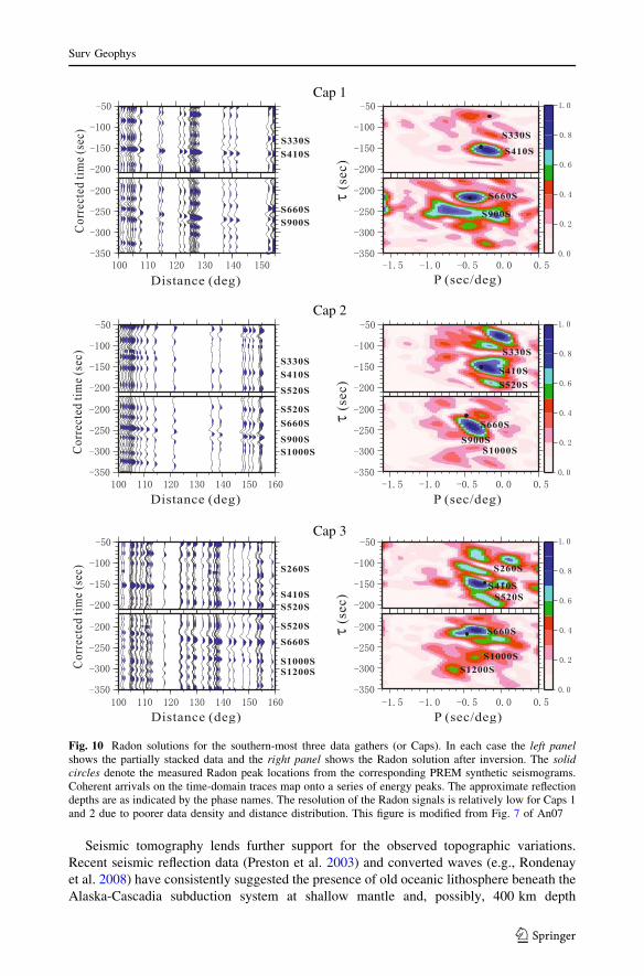
Seismic tomography lends further support for the observed topographic variations.

Recent seismic reflection data (Preston et al. 2003) and converted waves (e.g., Rondenay

et al. 2008) have consistently suggested the presence of old oceanic lithosphere beneath the

Alaska-Cascadia subduction system at shallow mantle and, possibly, 400 km depth

Cap 1

Cap 3

Cap 2

Fig. 10 Radon solutions for the southern-most three data gathers (or Caps). In each case the left panelshows the partially stacked data and the right panel shows the Radon solution after inversion. The solidcircles denote the measured Radon peak locations from the corresponding PREM synthetic seismograms.Coherent arrivals on the time-domain traces map onto a series of energy peaks. The approximate reflectiondepths are as indicated by the phase names. The resolution of the Radon signals is relatively low for Caps 1and 2 due to poorer data density and distance distribution. This figure is modified from Fig. 7 of An07

Surv Geophys

123

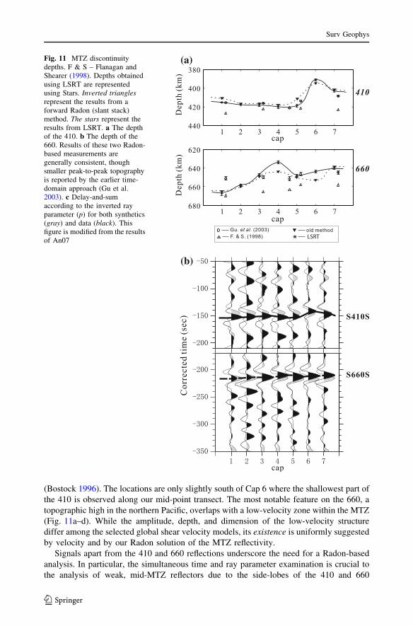
(Bostock 1996). The locations are only slightly south of Cap 6 where the shallowest part of

the 410 is observed along our mid-point transect. The most notable feature on the 660, a

topographic high in the northern Pacific, overlaps with a low-velocity zone within the MTZ

(Fig. 11a–d). While the amplitude, depth, and dimension of the low-velocity structure

differ among the selected global shear velocity models, its existence is uniformly suggested

by velocity and by our Radon solution of the MTZ reflectivity.

Signals apart from the 410 and 660 reflections underscore the need for a Radon-based

analysis. In particular, the simultaneous time and ray parameter examination is crucial to

the analysis of weak, mid-MTZ reflectors due to the side-lobes of the 410 and 660

(b)

(a)

LSRT

Fig. 11 MTZ discontinuitydepths. F & S – Flanagan andShearer (1998). Depths obtainedusing LSRT are representedusing Stars. Inverted trianglesrepresent the results from aforward Radon (slant stack)method. The stars represent theresults from LSRT. a The depthof the 410. b The depth of the660. Results of these two Radon-based measurements aregenerally consistent, thoughsmaller peak-to-peak topographyis reported by the earlier time-domain approach (Gu et al.2003). c Delay-and-sumaccording to the inverted rayparameter (p) for both synthetics(gray) and data (black). Thisfigure is modified from the resultsof An07

Surv Geophys

123

reflections (Shearer 1990, 1996; Gu et al. 1998; Deuss and Woodhouse 2001). We con-

fidently resolve the 520 beneath the Pacific portion of the mid-point gathers, but the

continental segment displays significant complexities and may imply multiple reflectors

within the MTZ (Deuss and Woodhouse 2001; Fig. 11e). The depth of the 520 appears to

weakly correlate with that of the 660, though the former exhibits significantly larger peak-

to-peak (45 km) topography than the latter (30 km; An07). The mean depth of 545 km is

slightly deeper than the reported value of 512 km based on earlier delay-and-sum analysis

(FS98). Other recognizable Radon peaks are associated with mantle depths of 250, 900,

1,050, and 1,150 km (see Fig. 12e for a summary).

4.5 HRT Analysis of Global Hotspots

The case study presented in Sect. 4.4 provides a blueprint for a global mapping of mantle

reflectors using RT-based imaging techniques. This section expands the scope of that pilot

study by exploring the seismic reflectivity structure beneath major hotspots using HRT, a

higher resolution approach based upon sparseness regularization constraints. The targets of

our analysis are 17 potentially ‘‘deep-rooted’’ hotspots (Courtillot et al. 2003) from a recent

global survey (Gu et al. 2009).

Questions regarding the genesis and depth extent of mantle plumes have persisted since

the hypothesis of mantle plumes was first formulated (Morgan 1971). Proposed global

catalogues based on geochemical and geophysical constraints (for reviews, see Courtillot

et al. 2003; Anderson 2005; Foulger 2007) have yet to fully reconcile the wide range of

surface expressions, mantle seismic wave speeds, buoyancy flux and isotopic compositions

among hotspots (Courtillot et al. 2003; Steinberger et al. 2004). From a seismic per-

spective, observations and interpretations differ substantially even for a widely studied

hotspot such as Iceland (e.g., Shen et al. 2002, 2003; Du et al. 2006). In other words, a self-

consistent explanation for the origin of globally distributed hotspots requires detailed maps

of both seismic velocity perturbations (e.g., Ritsema et al. 1999; Montelli et al. 2004; Zhou

et al. 2006) and discontinuity structures over a larger sample size. Results from shear and

compressional velocity inversions should normally be considered the first choice as mantle

thermometers, unfortunately, uncertainties at MTZ depths (400–700 km) remain the

Achilles’ heel in the plume debate due to insufficient resolution (e.g., Romanowicz 2003;

Ritsema et al. 2004). Secondary reflections and conversions offer a viable alternative in the

delineation of thermal variations and impedance contrasts across mantle reflectors beneath

hotspots (e.g., Li et al. 2000; Shen et al. 2003; Du et al. 2006).

For this part of the analysis we introduce averaging gathers beneath 17 potentially

‘‘deep-rooted’’ hotspots and seek common characteristics among them (see Fig. 9). The

data density is substantially higher than that shown in Sect. 4.4 despite larger averaging

areas. Sample Radon solutions of 6 hotspots (Fig. 13; see Gu et al. 2009) show a series of

highly focused Radon peaks throughout the mantle above 1,400 km. The resolution of the

Radon peaks is visibly higher than that presented by LSRT due to the use of sparseness

constraint on the solutions. Beneath most hotspots we record a stronger reflection from the

410 than from the 660: for example, the S410S Radon peak is 30–50% larger than S660S in

s-p domain beneath the Canary and Cape Verde hotspots. The s–p range of the two major

MTZ discontinuities is slightly smaller than that detailed in Sect. 4.4, thus suggesting less

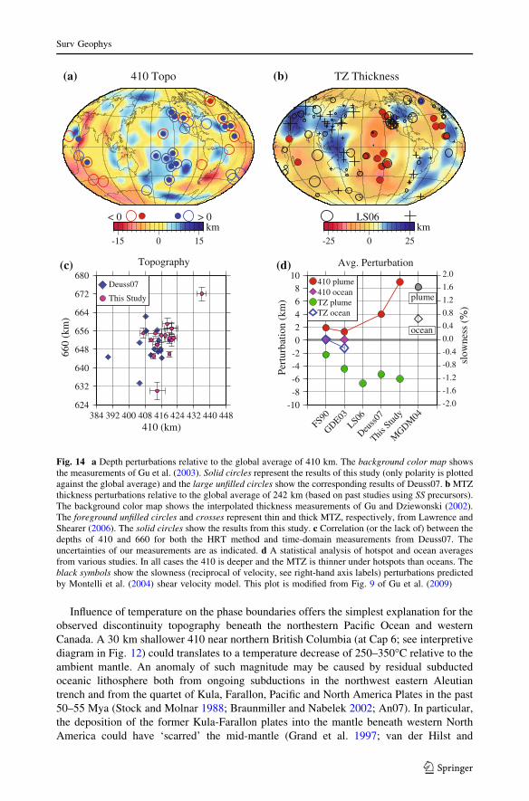
peak-to-peak topography. The inferred depth of the 410 (Fig. 14a) are generally consistent

with earlier results obtained by time–domain delay-and-sum (FS98; Gu et al. 2003;

Lawrence and Shearer 2006; Deuss07; Houser et al. 2008), while the MTZ (Fig. 14b) is

narrower than the global average of *240 km obtained using SS precursors (Gu et al.

Surv Geophys

123

(a) (b)

(c) (d)

(e)

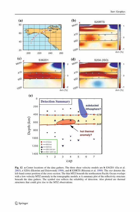
hot thermalanomaly?

Detection Summarysubductedlithosphere?

Fig. 12 a Center locations of the data gathers. The three shear velocity models are b S362D1 (Gu et al.2003), c S20A (Ekstrom and Dziewonski 1998), and d S20RTS (Ritsema et al. 1999). The star denotes theleft-hand corner position of the cross-section. The thin MTZ beneath the northeastern Pacific Ocean overlapswith a low-velocity MTZ anomaly in the tomographic models. e A summary plot of the reflectivity structurebeneath the data gathers. The symbol size reflects the reliability of detection. Also plotted are thermalstructures that could give rise to the MTZ observations

Surv Geophys

123

2003; Houser et al. 2008) due to a substantially depressed 410. The latter observation is

supported by a recent study of receiver functions (Lawrence and Shearer 2006), as well as

by 19 out of 26 hotspots examined in Deuss07. Figure 14d summarizes the main char-

acteristics of the MTZ beneath hotspots using a statistical comparison of several published

studies. In order to differentiate the ‘hotspot mantle’ from the average oceanic mantle, we

divide the Earth’s mantle based on the tectonic regionalization scheme of Jordan (1984)

and compare the median depths of the 410 under hotspots to the global and ocean averages.

While the depths of the two reflectors do not appear to correlate on the global scale

(Fig. 14c; Gu et al. 1998), the hotspot observations (the 410 depth, MTZ thickness) sys-

tematically differ from those pertaining to the average oceanic mantle (Fig. 14d). In

particular, the median 410 depths beneath hotspots are consistently deeper than the two

larger-scale averages, especially according to the two most recent studies where hotspots

are carefully targeted (Deuss07) and potentially better resolved (this study). Deep 410 and

thin MTZ beneath hotspots coincide with region of slow upper mantle velocities in PR5

model (Montelli et al. (2004) where the ‘hotspot’ mantle is, on average, 1% slower than

beneath the ‘‘normal’’ oceanic lithosphere (see Fig. 14d).

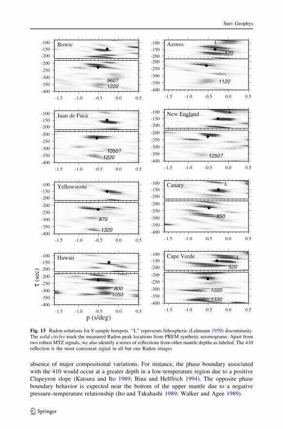
Similar to the northeastern Pacific path, the Radon solutions also show a slew of

reflections arising from the depth ranges of 200–350, 500–600, 800–920, and 1,000–

1,400 km (see Fig. 13). The simultaneous s–p constrains on these signals overcome

ambiguities (Neele and de Regt 1997) that typically hamper the time-domain efforts. The

HRT solution also appears sharper than the LSRT solution. The most notable signals arrive

in the time range of 80–120 s prior to SS. Their timing is regionally variable, as reflections

from most oceanic hotspots arrive closer to the surface reflection (SS) than hotspots near

continents (e.g., the Cape Verde and Canary hotspots). These ‘lithospheric’ (Lehmann

1959) reflectors are notably absent in Fig. 13 beneath the northeastern Pacific Ocean. In

comparison, signatures from a potential 520 are only reliably identified beneath hotspots in

the northern Atlantic Ocean (e.g., Azores, Cape Verde, and Canary hotspots, mostly close

to continents). The limited visibility of the 520, at *30% of the examined hotspots, is

inconsistent with the earlier reports of their global (Shearer 1990) or oceanic (Gu et al.

1998; Deuss and Woodhouse 2001; see Fig. 12e) presence.

The presence of shallow lower-mantle reflectors is confirmed by seismic phases arriving

220–300 s before SS. For example, the time series from the Louisville hotpot presents

multiple move-out curves that closely follow those produced by PREM. In general, the

amplitude and depth of these modest reflectors are highly variable (see Fig. 12e) and their

spatial distributions do not favor the oceans.

4.6 Abbreviated Interpretations and Discussions

The existence and depths of these reflectors could have significant implications for the

thermal and compositional stratification(s) within the mantle (e.g., Niu and Kawakatsu

1997; Deuss and Woodhouse 2002; Shen et al. 2003; see Sect. 4.5). In comparison with

time-domain approaches, the use of LSRT (Sect. 4.4) and HRT (Sect. 4.5) can lead to more

accurate assessments of the existence and depth variation of known and postulated seismic

reflectors. In both examples reflections from the 410 and 660 appear to be omnipresent, and

their occurrences have been widely attributed to solid–solid phase transitions from

a-olivine to wadsleyite (the former reflection; Katsura and Ito 1989) and from ringwoodite

to magnesiowustite ((Fe, Mg) O) and silicate perovskite ((Mg, Fe)SiO3) (the latter

reflection; Ringwood 1975; Ito and Takahashi 1989). Improved constraint on the depth and

reflection amplitude translates to more accurate estimates of mantle temperatures in the

Surv Geophys

123

absence of major compositional variations. For instance, the phase boundary associated

with the 410 would occur at a greater depth in a low-temperature region due to a positive

Clapeyron slope (Katsura and Ito 1989; Bina and Helffrich 1994). The opposite phase

boundary behavior is expected near the bottom of the upper mantle due to a negative

pressure–temperature relationship (Ito and Takahashi 1989; Walker and Agee 1989).

-200-150-100

-400

-350

-300

-250

-200

-1.5 -1.0 -0.5 0.0 0.5

Bowie

960?1220

-200-150-100

-400

-350

-300

-250

-200

-1.5 -1.0 -0.5 0.0 0.5

Juan de Fuca

1050?1220

-200-150-100

-400

-350

-300

-250

-200

-1.5 -1.0 -0.5 0.0 0.5

Yellowstone

870

1320

-200-150-100

-400

-350

-300

-250

-200

-1.5 -1.0 -0.5 0.0 0.5

Hawaii

τ (s

ec)

p (s/deg)

8001050

-200-150-100

-400

-350

-300

-250

-200

-1.5 -1.0 -0.5 0.0 0.5

Azores L

520

1120

-200-150-100

-400

-350

-300

-250

-200

-1.5 -1.0 -0.5 0.0 0.5

LNew England

1250?

-200-150-100

-400

-350

-300

-250

-200

-1.5 -1.0 -0.5 0.0 0.5

Canary L

850

-200-150-100

-400

-350

-300

-250

-200

-1.5 -1.0 -0.5 0.0 0.5

Cape Verde L

520

1020

1330

Fig. 13 Radon solutions for 8 sample hotspots. ‘‘L’’ represents lithospheric (Lehmann 1959) discontinuity.The solid circles mark the measured Radon peak locations from PREM synthetic seismograms. Apart fromtwo robust MTZ signals, we also identify a series of reflections from other mantle depths as labeled. The 410reflection is the most consistent signal in all but one Radon images

Surv Geophys

123

Influence of temperature on the phase boundaries offers the simplest explanation for the

observed discontinuity topography beneath the northestern Pacific Ocean and western

Canada. A 30 km shallower 410 near northern British Columbia (at Cap 6; see interpretive

diagram in Fig. 12) could translates to a temperature decrease of 250–350�C relative to the

ambient mantle. An anomaly of such magnitude may be caused by residual subducted

oceanic lithosphere both from ongoing subductions in the northwest eastern Aleutian

trench and from the quartet of Kula, Farallon, Pacific and North America Plates in the past

50–55 Mya (Stock and Molnar 1988; Braunmiller and Nabelek 2002; An07). In particular,

the deposition of the former Kula-Farallon plates into the mantle beneath western North

America could have ‘scarred’ the mid-mantle (Grand et al. 1997; van der Hilst and

-15 0 15

(a) 410 Topo

< 0 > 0km

-25 0 25

(b) TZ Thickness

LS06km

624

632

640

648

656

664

672

680

660

(km

)

384 392 400 408 416 424 432 440 448410 (km)

Deuss07

This Study

(c) Topography

-10-8-6-4-202468

10Pe

rtur

batio

n (k

m)

slow

ness

(%

)

-2.0

-1.6

-1.2

-0.8

-0.4

0.0

0.4

0.8

1.2

1.6

2.0410 plume410 oceanTZ plumeTZ ocean

FS90

GDE03LS06

Deuss0

7

This S

tudy

MGDM

04

plume

ocean

(d) Avg. Perturbation

Fig. 14 a Depth perturbations relative to the global average of 410 km. The background color map showsthe measurements of Gu et al. (2003). Solid circles represent the results of this study (only polarity is plottedagainst the global average) and the large unfilled circles show the corresponding results of Deuss07. b MTZthickness perturbations relative to the global average of 242 km (based on past studies using SS precursors).The background color map shows the interpolated thickness measurements of Gu and Dziewonski (2002).The foreground unfilled circles and crosses represent thin and thick MTZ, respectively, from Lawrence andShearer (2006). The solid circles show the results from this study. c Correlation (or the lack of) between thedepths of 410 and 660 for both the HRT method and time-domain measurements from Deuss07. Theuncertainties of our measurements are as indicated. d A statistical analysis of hotspot and ocean averagesfrom various studies. In all cases the 410 is deeper and the MTZ is thinner under hotspots than oceans. Theblack symbols show the slowness (reciprocal of velocity, see right-hand axis labels) perturbations predictedby Montelli et al. (2004) shear velocity model. This plot is modified from Fig. 9 of Gu et al. (2009)

Surv Geophys

123

Karason 1999) and littered in the upper mantle (Bostock 1996; An07; Courtier and Rev-

enaugh 2008). On the other hand, a hot thermal anomaly near the bottom of the upper

mantle is most likely responsible for the observed elevation of the 660 in the northeastern

Pacific Ocean (see Figs. 10 and 11). Although the depth of this low-velocity regime may

not be sufficiently resolved by the published global shear velocity models, its existence is

independently verified by the observed phase-boundary movement. Furthermore, its depth

should be is closer to the bottom, rather than the top, of MTZ in order to affect the local

depth of the 660. We refer the readers to An07 for in-depth discussions of the afore-

mentioned topographic features.

The HRT solution of the global hotspots paints a more complex mantle picture. While

the consistent depression and enhanced reflectivity of the 410 appear to be thermally

driven, a relatively weak and deep 660 is inconsistent with that expected of ringwoodite to

perovskite and magnesiowustite transformation under high temperatures. Mechanisms

involving water (Karato and Jung 1998; Bercovici and Karato 2003; Tonegawa et al.

2008), partial melt (e.g., Revenaugh and Sipkins 1994) and exothermic (heat-producing)

majorite to Ca-perovskite transition (e.g., Weidner and Wang 1998, 2000; Hirose 2002)

may be important. In fact, some of the so-called ‘660’ on the HRT solutions could, in truth,

reflect the transition of majorite garnet (rather than with the olivine) component of the

MTZ (Gu et al. 2009).

Finally, LSRT and HRT methods confidently resolve a number of weak reflectors away

from MTZ, with depths ranging from lithosphere to the mid mantle. Some of these

reflectors (e.g., the 220, 520) are notoriously difficult to quantify due to time-domain

waveform interference from stronger reflectors (e.g., surface, the 410 and 660; Deuss and

Woodhouse 2002; Neele and de Regt 1997), but the aforementioned difficulty can be

circumvented through signal isolation and enhancement in the transformed space. The

underlying message is that reflecting structures (see Figs. 10 and 13) are fairly common

beneath a wide range of tectonic regimes, including major hotspots and perceived ‘quiet’

oceanic regimes such as the northeastern Pacific region. Without entailing extensive details

on the interpretations (see Gu et al. 2009) it suffices to say that important inferences can be

made from global comparisons of reliable reflectivity images, especially images that satisfy

both travel time and ray angle constraints.

5 Conclusions

This study reviews the fundamentals and simple global seismic applications of Radon

transform. These methods can be equally effective on almost all short- or long-period

seismic waves that are quantifiable by linear, parabolic, or hyperbolic distance–time

relationships. Examples based on analysis of SS precursors show only a glimpse of the

elegance and flexibility of Radon solutions. From a broader perspective, the success of

Radon-based methods represents only a microcosm of contributions from many array/

exploration methods currently deployed in global seismology; a number of these methods

are detailed by the various contributions to this Special Issue. In short, many conceptual or

practical barriers that used to divide exploration and global seismic applications are no

longer withstanding. One could legitimately argue that exploration seismology is becoming

a realistic, scaled-down model for global surveys. With the help of ever-improving global/

regional seismic network coverage, greater successes of ‘global’ applications of many

other high-resolution, flexible ‘exploration’ techniques will not be a question of if, but a

matter of when.

Surv Geophys

123

Acknowledgments We sincerely thank Yuling An, Ryan Schultz and Jeroen Ritsma for their scientificcontributions and discussions. In particular, much of the work presented here was based on the MSc. thesisof Yuling An (currently at CGGVeritas) and an undergraduate summer project conducted by Ryan Schultz.We also thank IRIS for data archiving and dissemination. Some of the figures presented were prepared usingthe GMT software (Wessel and Smith 1995). Finally, we thank Surveys in Geophysics, particularly MichaelRycroft and Petra D. van Steenbergen, for inviting us to contribute to this Special Issue. The research projectis funded by Alberta Ingenuity, National Science and Engineering Council (NSERC) and CanadianFoundation for Innovations (CFI).

References

An Y, Gu YJ, Sacchi M (2007) Imaging mantle discontinuities using least-squares Radon transform.J Geophys Res 112:B10303. doi:10.1029/2007JB005009

Anderson DL (2005) Scoring hot spots: the plume and plate paradigms. In: GR Foulger, JH Natland, DCPresnall, DL Anderson (eds) Plates, plumes, and paradigms, Geol. Soc. Am. Special Volume 388, 31–54

Bassin C, Laske G, Masters MG (2000) The current limits of resolution for surface wave tomography inNorth America. EOS Trans, AGU, 81, Fall. Meet. Suppl. F897

Bercovici D, Karato S-J (2003) Whole mantle convection and the transition-zone water filter. Nature425:39–44

Beylkin G (1985) Imaging of discontinuities in the inverse scattering problem by inversion of a causalgeneralized radon transform. J Math Phys 26:99–108

Beylkin G (1987) Discrete radon transform. IEEE Trans Acoust 2:162–172 ASSP-2Bina CR, Helffrich GR (1994) Phase transition clapeyron slopes and transition zone seismic discontinuity

topography. J Geophys Res 99:15853–15860Bostock NG (1996) Ps conversions from the upper mantle transition zone beneath the Canadian landmass.

J Geophys Res 101:8393–8402Bracewell RN (1956) Strip integration in radio astronomy. Aust J Phys 9:198–201Braunmiller J, Nabelek J (2002) Seismotectonics of the explorer region. J Geophys Res 107:2208. doi:

10.1029/2001JB000220Chapman CH (2004) Fundamentals of seismic wave propagation. Cambridge University Press, p 632Clayton RW, McMechan GA (1981) Inversion of refraction data by wave field continuation. Geophysics

46:860–868Cormack AM (1963) Representation of a function by its line integrals, with some radiological applications.

J Appl Phys 34:2722–2727Courtier AM, Revenaugh J (2008) Slabs and shear wave reflectors in the midmantle. J Geophys Res

113:B08312. doi:10.1029/2007JB005261Courtillot V, Davaillie A, Besse J, Campbell IH (2003) Three distinct types of hotspots in the Earth’s

mantle. Earth Planet Sci Lett 205:295–308Davies D, Kelly EJ, Filson JR (1971) Vespa process for analysis of seismic signals. Nat Phys Sci 232:8–13Deuss A (2007) Seismic observations of transition-zone discontinuities beneath hotspot locations. In:

Foulger GR, Jurdy DM (eds) Plates, plumes and planetary processes, Geological Society Special Paper430, 121–136, doi: 10.1130/2007.2430(07)

Deuss A, Woodhouse JH (2001) Seismic observations of splitting of the mid-transition zone discontinuity inthe Earth’s mantle. Science 294:354–357

Deuss A, Woodhouse JH (2002) A systematic search for mantle discontinuities using SS-precursors.Geophys Res Lett 29:1–4

Du Z, Vinnik LP, Foulger GR (2006) Evidence from P-to-S mantle converted waves for a flat ‘‘660-km’’discontinuity beneath Iceland. Earth Planet Sci Lett 241:271–280

Dziewonski AM, Anderson DL (1981) Preliminary reference Earth model. Phys Earth Planet Inter25:297–356

Dziewonski AM, Gilbert F (1976) Effect of small, aspherical perturbations on travel times and re-exami-nation of the corrections for ellipticity. Geophys J R astr Soc 44:7–16

Escalante C, Gu YJ, Sacchi M (2007) Simultaneous iterative time-domain deconvolution to teleseismicreceiver functions. Geophys J Int 171:316–325. doi:10.1111/j.1365-246x.2007.03511.x

Estabrook H, Kind R (1996) The nature of the 660-kilometer upper-mantle seismic discontinuity fromprecursors to the PP phase. Science 274:1179–1182

Ekstrom G, Dziewonski AM (1998) The unique anisotropy of the Pacific upper mantle. Nature 394:168–172Flanagan MP, Shearer PM (1998) Global mapping of topography on transition zone velocity discontinuities

by stacking SS precursors. J Geophys Res 103:2673–2692

Surv Geophys

123

Foulger GR (2007) The ‘‘plate’’ model for the genesis of melting anomalies. Geol Soc Am 430:1–28 SpecialPaper

Gorman A, Clowes R (1999) Wave-field tau-p analysis for 2-D velocity models: application to westernNorth American lithosphere. Geophys Res Lett 26:2323–2326

Gossler J, Kind R (1996) Seismic evidence for very deep roots of continents. Earth Planet Sci Lett 138:1–13Grand SP, van der Hilst RD, Widiyantoro S (1997) Global seismic tomography: a snapshot of convection in

the Earth. GSA Today 7:1–7Gu YJ, Dziewonski AM, Agee CB (1998) Global de-correlation of the topography of transition zone

discontinuities. Earth Planet Sci Lett 157:57–67Gu YJ, Dziewonski AM (2002) Global variability of transition zone thickness. J Geophys Res 107:2135.

doi:10.1029/2001JB000489Gu YJ, Dziewonski AM, Ekstrom G (2003) Simultaneous inversion for mantle shear velocity and topog-

raphy of transition zone discontinuities. Geophys J Int 154:559–583Gu YJ, Dziewonski AM, Su W-J, Ekstrom G (2001) Models of the mantle shear velocity and discontinuities

in the pattern of lateral heterogeneities. J Geophys Res 106:11169–11199Gu YJ, An Y, Sacchi M, Schultz R, Ritsema J (2009) Mantle reflectivity structure beneath oceanic hotspots.

Geophys J Int. doi:10.1111/j.1365-246x.2009.04242.xHampson D (1986) Inverse velocity stacking for multiple elimination. J Can Soc Expl Geophys 22(1):44–55Hirose K (2002) Phase transitions in pyrolitic mantle around 670-km depth: implications for upwelling of

plumes from the lower mantle. J Geophys Res 107:2078. doi:10.1029/2001JB000597Houser C, Masters G, Flanagan GM, Shearer PM (2008) Determination and analysis of long-wavelength

transition zone structure using SS precursors. Geophys J Int 174:178–194. doi:10.111/j.1365-246X.2008.03719.x

Ito E, Takahashi E (1989) Postspinel transformations in the system Mg2SiO4–Fe2SiO4 and some geophysicalimplications. J Geophys Res 94:10637–10646

Kappus ME, Harding AJ, Orcutt J (1990) A comparison of tau-p transform methods. Geophysics 55:1202.doi:10.1190/1.1442936

Karato S-I, Jung H (1998) Water, partial melting and the origin of the seismic low velocity and highattenuation zone in the upper mantle. Earth Planet Sci Lett 157:193–207

Katsura T, Ito E (1989) The system Mg2SiO4–Fe2SiO4 at high pressures and temperatures; precise deter-mination of stabilities of olivine, modified spinel, and spinel. J Geophys Res 94:15663–15670

Kawakatsu H, Watada S (2007) Seismic evidence for deep water transportation in the mantle. Science316:1468–1471

Kruger F, Weber M, Scherbaum F, Schittenhardt J (1993) Double beam analysis of anomalies in the core-mantle boundary region. Geophys Res Lett 20:1475–1478

Lawrence JF, Shearer PM (2006) A global study of transition zone thickness using receiver functions.J Geophys Res 111:B06307. doi:10.1029/2005JB003973

Lehmann I (1959) Velocities of longitudinal waves in the upper part of the Earth’s mantle. Geophys J RAstron Soc 15:93–113

Li X, Kind R, Priestley K, Sobolev SV, Tilmann F, Yuan X, Weber M (2000) Mapping the Hawaiian plumeconduit with converted seismic waves. Nature 427:827–829

Ma P, Wang P, De Hoop MV, Tenorio L, Van der Hilst RD (2007) Imaging of structure at and near the core-mantle boundary using a generalized radon transform: 2. Statistical inference of singularities. J GeophysRes 112:B08303. doi:10.1029/2006JB004513

Menke W (1989) Geophysical data analysis: discrete inverse theory. Academic Press Inc., San Diego, p 289Miller D, Oristaglio M, Beylkin G (1987) A new slant on seismic imaging: migration and integral geometry.

Geophysics 52(7):943–964Montelli R, Nolet G, Dahlen FA, Masters G, Engdah ER, Hung SH (2004) Finite-frequency tomography

reveals a variety of plumes in the mantle. Science 303:338–343Morgan WJ (1971) Convection plumes in the lower mantle. Nature 230:42–43Neele F, de Regt H (1997) Imaging upper-mantle discontinuity topography using underside-reflection data.

Geophys J Int 137(1):91–106Niu F, Kawakatsu H (1995) Direct evidence for the undulation of the 660-km discontinuity beneath Tonga:

comparison of Japan and California array data. Geophy Res Lett 22(5):531–534Niu F, Kawakatsu H (1997) Depth variation of the mid-mantle seismic discontinuity. Geophys Res Lett

24(4):429–432Papoulis A (1962) The Fourier integral and its applications. McGraw-Hill, New YorkParker RL (1994) Geophysical inverse theory. Princeton University Press, Princeton, p 386Preston LA, Creager KC, Crosson RS, Brocher TM, Trehu AM(2003) Intraslab earthquakes: dehydration of

the Cascadia slab. Science302(5648):1197–1200. doi:10.1126/science.1090751

Surv Geophys

123

Radon J (1917) Uber die Bestimmung von Funktionen durch ihre Integralverte langs gewiusser Manni-gfaltigkeiten, Berichte Sachsische Academie der Wissenschaften, Leipzig. Math Phys Kl 69:262–267

Revenaugh J, Sipkin SA (1994) Seismic evidence for silicate melt atop the 410-km mantle discontinuity.Nature 369:474–476

Ringwood AE (1975) Composition and petrology of the earth’s mantle. McGraw-Hill, New York, p 630Ritsema J, Van Heijst HJ, Woodhouse JH (1999) Complex shear wav velocity structure imaged beneath

Africa and Iceland. Science 286:1925–1928Ritsema JH, van Heijst J, Woodhouse JH (2004) Global transition zone tomography. J Geophys Res

109:B02302. doi:10.1029/2003JB002610Romanowicz B (2003) Global mantle tomography: progress status in the last 10 years. Annu Rev Geophys

Space Phys 31(1):303Rondenay S, Abers G, van Keken P (2008) Seismic imaging of subduction metamorphism. Geology

36(4):275–278. doi:10.1030/G24112ARost S, Garnero E (2004) A study of the uppermost inner core from PKKP and P’P’ differential travel times.

Geophys J Int 156:565–574. doi:10.1111/j.1365-246X.2004.02139.xRost S, Thomas C (2002) Array seismology: methods and applications. Reviews of Geophysics 40: 2-1–2-

27. doi:10.1029/2000RG000100Sacchi M, Ulrych TJ (1995) High-resolution velocity gathers and offset space reconstruction. Geophysics

60:1169–1177Schmerr N, Garnero EJ (2006) Investigation of upper mantle discontinuity structure beneath the central

Pacific using SS precursors. J Geophys Res 111:B08305. doi:10.1029/2005JB004197Shearer PM (1990) Seismic imaging of upper-mantle structure with new evidence for a 520-km disconti-

nuity. Nature 344:121–126Shearer PM (1991) Imaging global body-wave phases by stacking long-period seismograms. J Geophys Res

96:20353–20364Shearer PM (1993) Global mapping of upper mantle reflectors from long-period SS precursors. Geophys

J Int 115:878–904Shearer PM (1996) Transition zone velocity gradients and the 520-km discontinuity. J Geophys Res

101:3053–3066Shearer PM (1999) Introduction to seismology. Cambridge Univ. Press, Cambridge, p 260Shen Y et al (2002) Seismic evidence for a tilted mantle plume and north-south mantle flow beneath Iceland.

Earth Planet Sci Lett 197:262–272Shen Y, Wolfe CJ, Solomon SC (2003) Seismological evidence for a mid-mantle discontinuity beneath

Hawaii and Iceland. Earth Planet Sci Lett 214:143–151Steinberger B, Sutherland R, O’Connell RJ (2004) Prediction of emperor-Hawaii seamount locations from a

revised model of global plate motion and mantle flow. Nature 430:167–173Stock JM, Molnar P (1988) Uncertainties and implications of the Cretaceous and Tertiary position of North

America relative to Farallon, Kula, and Pacific plates. Tectonics 7:1339–1384Su WJ, Woodward RL, Dziewonski AM (1994) Degree-12 model of shear velocity heterogeneity in the

mantle. J Geophys Res 99:6945–6980Tauzin B, Debayle E, Wittlinger G (2008) The mantle transition zone as seen by global Pds phases: no clear

evidence for a thin transition zone beneath hotspots. J Geophys Res 113:B08309. doi:10.1029/2007JB005364

Thorson J, Claerbout J (1985) Velocity-stack and slant-stack stochastic inversion. Geophysics 50:2727–2741

Tonegawa T, Hirahara K, Shibutani T, Takuo S, Iwamori IH, Kanamori H, Shiomi K (2008) Water flow tothe mantle transition zone inferred from a receiver function image of the Pacific slab. Earth Planet SciLett 274:346–354. doi:10.1016/j.epsl.2008.07.046

Trad D, Ulrych TJ, Sacchi M (2002) Accurate interpolation with high-resolution time-variant Radontransforms. Geophysics 67:644–656

van der Hilst RD, Karason H (1999) Compositional heterogeneity in the bottom 1000 kilometers of Earth’smantle: toward a hybrid convection model. Science 286:1925–1928

Vidale JE, Benz HM (1992) Upper-mantle seismic discontinuities and the thermal structure of subductionzones. Nature 356:678–683

Walker D, Agee C (1989) Partitioning ‘‘equilibrium’’, temperature gradients, and constraints on Earthdifferentiation. Earth Planet Sci Lett 96:49–60

Wang P, De Hoop MV, Van der Hilst RD, Ma P, Tenorio L (2006) Imaging of structure at and near the coremantle boundary using a generalized Radon transform: 1- construction of image gathers. J GeophysRes 111, B12, B12304. doi:10.1029/2005JB004241

Surv Geophys

123

Wessel P, Smith WHF (1995) The generic mapping tools (GMT) version 3.0 Technical Reference &Cookbook, SOEST/NOAA

Wilson CK, Guitton A (2007) Teleseismic wavefield interpolation and signal extraction using high reso-lution linear radon transforms. Geophys J Int 168:171–181

Weidner DJ, Wang Y (1998) Chemical and Clapeyron-induced buoyancy at the 660 km discontinuity.J Geophys Res 103:7431–7441

Weidner DJ, Wang Y (2000) Phase transformations: implications for mantle structure. In: Karato S et al(eds) Earth’deep interior: mineral physics and tomography from the atomic to the global scale.Geophys. Monogr. Ser, vol 117. AGU, Washington, D. C, pp 215–235

Yilmaz O (1987) Seismic Data Processing. Soc Expl Geophys, Tulsa (Oklahoma), p 526Zhou Y, Nolet G, Dahlen FA, Laske G (2006) Global upper-mantle structure from finite-frequency surface

wave tomography. J Geophys Res 111:B04304. doi:10.1029/2005JB003677

Surv Geophys

123