Embed Size (px)
Citation preview
Radar Alignment and Accuracy Tool RASS-R Radar Comparator Dual
Edition: 2 Date: 10-Aug-09 Status: Released
Radar Alignment and Accuracy Tool: RASS-R Radar Comparator Dual 2/53
DOCUMENT DESCRIPTION
Document Title Radar Alignment and Accuracy Tool: RASS-R Radar Comparator Dual
2 Edition 10-Aug-09 Edition date Andrey Pchelintsev (Ph.D, R&D Scientist) Author Dirk De bal (System engineer) and Marcel Vanuytven (CEO)
Editor
Abstract
This document describes the general principles underlying the Radar Comparator Dual, demonstrates results of various evaluation campaigns, discuss the main outcomes of the technique for the accurate analysis of modern radar hardware. A special attention has been paid to using of ADS-B data for radar analysis, evaluation and continuous monitoring.
Keywords Multi-radar alignment Accuracy Figure of Merit ADS-B radome 3D radar OBA lookup table
Andrey Pchelintsev +32 14 231811 Contact person Tel
[email protected] address
DOCUMENT STATUS
STATUS Working Draft Draft Proposed Issue Released Issue
ELECTRONIC BACKUP
IE-SUP-00042-002 Radar Alignment and Accuracy Tool.doc INTERNAL REFERENCE NAME : HOST SYSTEM SOFTWARE(S) Windows XP Pro Word 2003
Radar Alignment and Accuracy Tool: RASS-R Radar Comparator Dual 3/53
DOCUMENT CHANGE RECORD Te following table records the complete history of the successive editions of the present document.
EDITION DATE REASON FOR CHANGE SECTIONS
PAGES AFFECTED
APPROVED BY
1.0 24-Nov-08 New document All AP
1.1 18-Feb-09 New Layout All EV
2 10-Aug-09 Updated version for publishing paper for 54th ATCA Annual Conference and Exposition; Section 4.8 removed; Chapter 5 added;
All AP BS
Radar Alignment and Accuracy Tool: RASS-R Radar Comparator Dual 4/53
TABLE OF CONTENTS
1. EXECUTIVE SUMMARY .......................................................................................................................... 9
2. INTRODUCTION..................................................................................................................................... 10
3. RADAR COMPARATOR NEW APPROACH ......................................................................................... 11 3.1 RADAR VS RADAR MEASUREMENT: BASIC PRINCIPLES ....................................................................... 11 3.2 USED METHODS ............................................................................................................................... 12 3.3 SYSTEMATIC ERRORS MEASUREMENT ............................................................................................... 12
3.3.1 Two Radars – Absolute Measurement ...................................................................................... 13 3.3.2 Two Radars – Relative Measurement ....................................................................................... 13 3.3.3 Accuracy of the Measurement ................................................................................................... 14 3.3.4 Radar vs. ADS-B Analysis ......................................................................................................... 15 3.3.5 Radar vs. ADS-B Analysis: Data Handling ................................................................................ 16
3.4 TRAJECTORY RECONSTRUCTION AND ACCURACY MEASUREMENT ....................................................... 19 4. RESULTS AND APPLICATIONS ........................................................................................................... 23
4.1 CASE A: REAL VALUE FOR RADAR EVALUATION AND CONTINUOUS PERFORMANCE MONITORING ......... 23 4.2 BAROMETRIC HEIGHT ERROR AND ADS-B ......................................................................................... 25 4.3 CASE B: RADAR RADOME INFLUENCE EVALUATION AND MONOPULSE DISTORTION CORRECTION ......... 28 4.4 CASE C: MEASUREMENT OF THE AZIMUTH ERRORS GENERATED BY LIGHTENING POLES...................... 32 4.5 CASE D: 3D RADAR ELEVATION OBA LOOKUP TABLES CORRECTION ................................................. 34 4.6 MEASUREMENT OF MODE-S AZIMUTH BIAS AT HIGH ELEVATION ANGLES ............................................ 35 4.7 AC ADS-B QUALITY MONITORING ..................................................................................................... 36
5. CONCLUSION ........................................................................................................................................ 37
6. ANNEX 1: RADAR COMPARATOR DUAL USED METHODS ............................................................. 38 6.1 DATA CORRECTION METHODS ........................................................................................................... 38
6.1.1 Timestamp Analysis ................................................................................................................... 38 6.1.2 ACP Eccentricity Correction ....................................................................................................... 38 6.1.3 Barometric Height Correction using Atmospheric Soundings .................................................... 38 6.1.4 Atmospheric Refraction Error and Correction ............................................................................ 39
6.2 GENERAL RADAR DATA PROCESSING METHODS ................................................................................ 42 6.2.1 XYZ-t Filtering Method ............................................................................................................... 42 6.2.2 Linear Interpolation .................................................................................................................... 42 6.2.3 Correlation of the Data ............................................................................................................... 43 6.2.4 Height Reconstruction ................................................................................................................ 43
6.3 RADAR VS. RADAR ANALYSIS ............................................................................................................ 43 6.3.1 Systematic Errors Measurement................................................................................................ 43 6.3.2 Matrix Structure .......................................................................................................................... 44 6.3.3 Relative Measurement ............................................................................................................... 47
6.4 RADAR VS. ADS-B ANALYSIS ............................................................................................................ 48 6.4.1 Matrix Structure .......................................................................................................................... 48 6.4.2 Measurement Figure of Merit (MFM) ......................................................................................... 50 6.4.3 Dual Comparison: Accuracy of the Measurement of the Systematic Errors ............................. 50
6.5 TRAJECTORY RECONSTRUCTION AND RANDOM ERRORS .................................................................... 51 7. REFERENCES........................................................................................................................................ 53
Radar Alignment and Accuracy Tool: RASS-R Radar Comparator Dual 5/53
TABLE OF FIGURES Figure 1: Results of aircraft latency measurement for four radars (Mode-S rad1, rad2 and SSR rad3, rad4) compared in 4 separate measurement campaigns to the same ADS-B data set ........................................... 16 Figure 2: Mode-S radars compared to the same ADS-B data set. Comparison between the inferred latencies and transponder delays. .................................................................................................................................. 17 Figure 3: Examples of the trajectories having different MFM: a) 9, b) 4, c) 0 ................................................. 18 Figure 4: Along track ADS-B errors for 3 aircraft calculated comparing ADS-B with rad1 (white line) and then with rad2 (red line). .......................................................................................................................................... 20 Figure 5: Examples of the trajectory reconstruction: a), c) speed variation, b), d) heading variation ............. 21 Figure 6: XY display: example of the high quality of the trajectory reconstruction .......................................... 22 Figure 7: Results of a 5-day continuous measurement including 2 MSSR, 3 MODES and ADS-B: azimuth bias dynamics for radar MODES#3 measured separately vs. different sources. ............................................ 24 Figure 8: Results of a 5-day continuous measurement including 2 MSSR radars, 3 MODES radars and ADS-B: range bias dynamics for radar MODES#3 measured separately vs. different sources. ............................. 24 Figure 9: Distribution of the barometric error for [5000, 5500] m measured 12:00pm to 12:00am on 24-01-2008 BELGOCONTROL .................................................................................................................................. 25 Figure 10: Distribution of the barometric error for [7000, 7500] m measured 12:00pm to 12:00am on 24-01-2008 BELGOCONTROL .................................................................................................................................. 26 Figure 11: Distribution of the barometric error for [9000, 9500] m measured 12:00pm to 12:00am on 24-01-2008 BELGOCONTROL .................................................................................................................................. 26 Figure 12: Distribution of the barometric error for [9000, 9500] m measured 12:00pm to 12:00am on 25-01-2008 BELGOCONTROL .................................................................................................................................. 27 Figure 13: Distribution of the barometric error for [9000, 9500] m measured 12:00pm to 12:00am on 26-01-2008 BELGOCONTROL .................................................................................................................................. 27 Figure 14: Picture of radar N. .......................................................................................................................... 28 Figure 15: Azimuth error vs. azimuth for radar N inside a radome ................................................................. 29 Figure 16: Gyro measurement for radar N showing ACP glitch ...................................................................... 29 Figure 17: Azimuth error vs. azimuth for radar N inside a radome after ACP eccentricity correction ............. 30 Figure 18: Gyro measurement for radar N showing ACP glitch ...................................................................... 30 Figure 19: Azimuth error vs. azimuth for radar N inside a radome after ACP eccentricity and radome distortion correction) ........................................................................................................................................ 31 Figure 20: Radar K: picture and the satellite image (Google Earth) ............................................................... 32 Figure 21: Average azimuth error vs. azimuth for radar K .............................................................................. 33 Figure 22: ADS-B elevation angle measurement noise vs. range .................................................................. 34 Figure 23: Azimuth bias vs. the elevation angle for MSSR and Mode-S radars ............................................. 35
Radar Alignment and Accuracy Tool: RASS-R Radar Comparator Dual 6/53
Figure 24: ADS-B latency measurements for 6 aircraft performed from January 23rd to January 26th 2008 36 Figure 25: ADS-B latency histogram built using 6 radars measurement vs. ADS-B performed from January 23rd to January 26th 2008. .............................................................................................................................. 37 Figure 26: Barometric height measurement and correction method ............................................................... 39 Figure 27: Calculation of the refraction ............................................................................................................ 40 Figure 28: The family of the refraction correction curves computed according to expression (14) vs. the exact computation according to formula (11)-(13). ................................................................................................... 41 Figure 29: Two-plot setup for the minimization procedure .............................................................................. 46 Figure 30: Principle of the trajectory reconstruction (search for the maximum likelihood function given the radar measurements and expected radar accuracy) ....................................................................................... 52
TABLE OF TABLES
Table 1: Advantages using ADS-B data for radar evaluation .......................................................................... 15 Table 2: Disadvantages and possible solutions in case of using ADS-B data for radar evaluation ................ 15
Radar Alignment and Accuracy Tool: RASS-R Radar Comparator Dual 7/53
GLOSSARY OF TERMS ACP Azimuth Change Pulse ADS-B Automatic Dependent Surveillance, Broadcast Annex 10 Aeronautical Telecommunication, Annex 10 to the Convention on
International Civil Aviation, the principle international document defining SSR
ARP Azimuth Reference Pulse ATC Air Traffic Control COTS Commercial Off The Shelf CPU Computer Processing Unit CW Continuous wave dB Decibel Downlink The signal path from aircraft to ground FL Flight Level, unit of altitude (expressed in 100’s of feet) FRUIT False Replies Unsynchronized In Time, unwanted SSR replies
received by an interrogator which have been triggered by other interrogators
GPS Global Positioning System ICAO International Civil Aviation Organization ICD Interface Control Document IE Intersoft Electronics IF Intermediate Frequency I/O Input/Output IP Internet Protocol LAN Local Area Network LVA Large Vertical Aperture (antenna) Monopulse Radar-receiving processing technique used to provide a precise
bearing measurement MSSR Monopulse Secondary Surveillance Radar MTD Moving Target Detection MTI Moving Target Indicator Multipath Interference and distortion effects due to the presence of more than
one path between transmitter and receiver NM Nautical Mile, unit of distance OEM Original Equipment Manufacturer Plot extractor Signal-processing equipment which converts receiver video into
digital target reports suitable for transmission by land lines PPI Plan Position Indicator PRF Pulse Repetition Frequency PSR Primary Surveillance Radar Radar Radio Detection And Ranging Radome Radio-transparent window used to protect an antenna principally
against the effects of weather RASS-R Radar Analysis Support Systems – Real-time measurements RASS-S Radar Analysis Support Systems – Site measurements RCS Radar Cross Section RDP Radar Data Processing (system) RF Radio Frequency RTQC Real Time Quality Control RX Receiver SAC System Area Code SIC System Identification Code SLS Side Lobe Suppression, a technique to avoid eliciting transponder
replies in response to interrogations transmitted via antenna sidelobes
SLB Side Lobe Blanking SNR Signal-to-Noise ratio
Radar Alignment and Accuracy Tool: RASS-R Radar Comparator Dual 8/53
Squitter Random reply by a transponder not triggered by an interrogation SSR Secondary Surveillance Radar STC Sensitivity Time Control TACAN Tactical Air Navigation TCP Transmission Control Protocol TIS-B Traffic Information Services, Broadcast Transponder Airborne unit of the SSR system, detects an interrogator’s
transmission and responds with a coded reply stating either the aircraft’s identity or its flight level
TX Transmitter Uplink Ground-to-air signal path UTC Coordinated Universal Time
Radar Alignment and Accuracy Tool: RASS-R Radar Comparator Dual 9/53
1. Executive Summary Automatic Dependent Surveillance Broadcast (ADS-B) is a surveillance technique that relies on the aircraft to broadcast their identity, position and other aircraft information. ADS-B is currently under investigation for implementation by EUROCONTROL's CASCADE and F.A.A.'s NextGen programs. Intersoft Electronics investigates the usage of ADS-B data in measurement techniques for radar evaluation (measurement of systematic and random errors). This paper shows the results of radar measurements vs. ADS-B using various evaluation techniques and discusses the main outcomes of the technique for the accurate analysis, measurement and improvement of modern ATC radar hardware. ADS-B data broadcasted by aircraft represents a great value for the radar evaluation, monitoring and correction. However not every ADS-B message can be used for the measurement, less accurate data must be distinguished and carefully discarded from the analysis. Even the remaining “good” data subset can’t be used directly, the ADS-B being subject to the specific effects and parameters as for example the latency. Curiously the ±0.25µs and ±0.5µs delay deviations allowed for aircraft transponders can also be measured and handled to results in unprecedented accuracy and consistency on the radar measurements. Using the methods of multi-parameter optimization Intersoft Electronics has developed a tool that can model both radar and ADS-B data for radar analysis. This model inherited the methods used by MURATREC (EUROCONTROL SASS-C) for multi-radar measurement and adapted these to the case of a two-source measurement (implemented in the RADAR Comparator Dual). Limiting the problem to two sources has produced an immediate benefit by making the measurement more controllable and accurate. With the ADS-B data already available from 50÷75% of modern aircraft the improvement in the Radar Comparator Dual monitoring capability and accuracy can be called spectacular. In this paper, we demonstrate the superior accuracy of the radar measurement using ADS-B data. However the tool can be used in the original mode if no ADS-B data are available, i.e. radar to radar evaluation mode. In general radar performance analysis with RADAR Comparator Dual starts with the measurement of all the known errors (barometric height measurement and atmospheric refraction for example) and if required corrections can be applied. Timestamp quality is routinely checked. If required, ACP eccentricity is corrected using the RASS-S gyro measurement data. The Radar Comparator Dual greatly benefits from using the radar measurements performed by the RASS-S software tools to find trends in the processed data. This represents a very powerful technique to establish the true sources of radar problems. A number of direct applications are demonstrated, such as continuous monitoring of radar alignment; precision measurement of the azimuth error due to the mono-pulse distortions caused by a radome or/and lightning rods; and of the azimuth bias increase for a Mode-S radar due to the antenna beam widening; the dramatic improvement of the elevation measurement accuracy by 3D radar. The side product of the radar vs. ADS-B evaluation is a valid method of the ADS-B evaluation and monitoring. Availability of more accurate measurement techniques has been always beneficial for the technological progress because it generally helps out to improve the existing technology. At the same time, the discussed methods create a real proposal for valid correction techniques.
Radar Alignment and Accuracy Tool: RASS-R Radar Comparator Dual 10/53
2. Introduction The idea of combining multi-radar data for radar alignment and accuracy measurement first appeared about 25 years ago as a result of the significant progress in radar technology and manufacturing and the public demand for the enhanced air traffic (AT) safety in the conditions of continuously increasing AT density. As a response to this requirement stipulated by EUROCONTROL Agency in 1982 in the public tender for a multi-radar measurement and evaluation software, SASS-C with MURATREC-1 (MUlti-RAdar TRajectory REconstruction) being its first measurement core has been developed. MURATREC gave to the radar engineers a method to evaluate radars (the systematic and random errors) using multi-radar data and mathematical model allowing for a number of the systematic errors (biases) and random errors (accuracy). The tool was developed by NRL (Nederland) and became operational during 1987-1990. In order to improve the poor quality of the trajectory reconstruction and therefore exaggerated error figures, the second version of the measurement core was developed by 1994 (MURATREC-2), then TR3 (also called MURATREC-3) prototype development has been funded for a while without significant breakthrough. Despite considerable amount of time and money spent for the development and maintenance of the tool, the SASS-C still fails to play the role it initially was assigned to. The most upsetting is that despite all the efforts the system doesn’t meet requirements for being a valid measurement tool. After more that 20 years of development it is still a prototype demonstrating poor performance. A number of problems with SASS-C have been technical. However the general drawback is conceptual: the lack of visibility of the data flow, so that it is impossible to find out, what actually causes a specific problem. Another drawback is the typically high count of the measured parameters, therefore high probability of the parameter cross-contamination, unknown accuracy of the parameter evaluation, and vague principles of the parameter selection. In other words there is no vision what the method should be able to measure and what not because it is impossible from the physics standpoint. It has been assumed that the more radars are used for the measurement, the better. However with noisy data multi-parameter optimization problem may often be compromised by the errors correlation, inadequate models and therefore non-Gaussian error distribution. It has been assumed as well that the data sets should be “balanced”, however no quantitative parameter that would indicate that the data set in balanced or unbalanced has ever been proposed. Unfortunately radar engineers have no control over balancing air traffic for the purpose of the measurement. “The more the better” doesn’t work for SASS-C, for more data without rigorous selection and checking of all the possible sources of errors create more chance for cross-contamination of data and unstable results etc. “The more the better” doesn’t work for a non-“balanced” setup, for in a multi-parameter minimization problem a number of the parameters happen to have correlated errors and can’t be measured separately. Since there was no method to test the ill-conditioning of a particular measurement setup, the accuracy of the measurement remains unknown, so that SASS-C can not be considered as a valid measurement tool.
Radar Alignment and Accuracy Tool: RASS-R Radar Comparator Dual 11/53
3. Radar Comparator New Approach Using the opposite approach “the less the better”, a new tool RADAR Comparator Dual has been developed by Intersoft Electronics NV, which processes data from two sources at a time. The analysis starts with measurement of all the known errors (barometric height measurement and atmospheric refraction for example) and if required corrections can be applied, timestamp quality is routinely checked, ACP eccentricity corrected if required using RASS-S gyro measurement data. The RADAR Comparator Dual greatly benefits of using RASS-S software tools to find trends in the data. This is a very powerful investigation technique that can be used to establish the true source of a problem. The basic principles of the measurement are presented in the next section.
3.1 Radar vs Radar Measurement: Basic Principles It is explicitly assumed the following: 1. Radars positions must be known to within 5m (absolute maximum positional error), so that the positional
uncertainty doesn’t affect accuracy of the measurement of the systematic and random errors of the radar. The position of the radar is fixed and never used as a parameter.
2. Only suitable traffic must be used for the measurement, i.e. aircraft maintaining conservative type of the
motion. Aircraft with non-conservative modes of motion should be discarded from both systematic error and accuracy measurement.
3. There exist physical limitations for the alignment and accuracy measurement depending on a particular
setup or “constellation” of two radars (sources), depending on the amount, and the pattern of the air traffic, and the individual accuracy of the radars. For example an absolute measurement of the alignment of two radars is possible only if the measurement system is not a singular or an ill-conditioned one. The condition number of the system matrix is the ratio between the largest and the smallest singular values. If the condition number is infinite the matrix is singular, and it can not be resolved. If the condition number is too large the measurement accuracy is poor. The accuracy of the measurement can be estimated by the noise covariance matrix (see sections 3.3.1 and 3.3.3). Technically when the radars are offset by a distance which is not too small and not too large, the systematic and random errors will be determined separately for both radars. Except for the time bias which is a relative measure.
4. For two co-located radars when the system matrix becomes singular or ill-conditioned, only relative measurements are possible.
5. For an absolute measurement involving two radars, typically 7 parameters are introduced
1212121 comprising 2 range biases, 2 range gains, 2 azimuth biases and the
relative time bias. The system matrix consists of a quantity (vector) to minimize in its right hand side and the partial derivatives of its components by each of the 7 parameters in its left side. The solution is found iteratively using matrix inversion techniques.
,,,,,, tθθKKRR ΔΔΔΔΔ
6. For the trajectory reconstruction the following method is used. The data processed per trajectory. For
each trajectory the following quantities are minimized being the target speed noise and range and azimuth accuracy of the radars. For more accurate results maneuvering segments of the trajectories should be discarded.
2211 ,,,,, θRθRVV yx ΔΔΔΔΔΔ
7. Poor timestamp quality is a source of additional positional and measurement errors. Timestamp quality
should be checked before using the data for the analysis. Timestamp errors may be corrected in order to investigate possible contamination of the biases and accuracy.
8. Barometric height measurement has been shown to induce large errors in cases when the local
atmospheric conditions are different from the ICAO Standard Atmosphere. The atmospheric balloon soundings used for the weather forecast routinely take place once or twice a day in many countries across the globe, are a good testimony of magnitude of the phenomenon. It has been shown that in extreme cases the height deviations can be of 1500m, however deviations of 500m are being more common. For two-radar setup the erroneous height data affects the predicted aircraft positions and thus inferred radar biases and accuracy. Radar data can be easily corrected using the balloon sounding data,
Radar Alignment and Accuracy Tool: RASS-R Radar Comparator Dual 12/53
and as it has been shown this correction is always beneficial. However this is a first order correction only because the pressure distribution seldom happens to be uniform over large measurement areas. ADS-B data is free of this type of error providing the true MSL height which is extremely important for radar evaluation purposes.
The RADAR Comparator Dual was carefully redesigned to use ADS-B data for radar alignment and random errors measurement.
3.2 Used Methods Prior to the evaluation the timestamp accuracy must be tested. Since the correct timing is as important for the accurate positional reconstruction as the range and azimuth, first timestamp data vs. azimuth is analyzed (see section 6.1.1). The data originating from the different sources must be processed in order to associate them with the same targets. An efficient and fast method to correlate data taken from two sources may use 3/A-code or S-address. Sources producing different data types (for example PSR vs. SSR, PSR vs. MODES, ADS-B vs. SSR etc.) require more effort for the correlation process. In those cases the association relies more on the target position, and its dynamics. For details please refer to section 6. In general the data taken by different sources are asynchronous. For the measurement purposes one needs to bring the samples to the same time, to do so general interpolation methods are used (see section 6.2.2).
3.3 Systematic Errors Measurement The dual radar comparison is typically used in order to determine the systematic errors of the both sources (radars or ADS-B). The systematic errors for radars include range bias, range gain, azimuth bias and time bias. The aircraft transponder delay variations are usually ignored in multi-radar analysis. The systematic errors for ADS-B may include the ADS-B latency and the transponder delay variations. The measurement algorithm assumes that all the measured parameters are described by the normal distribution law. Two first statistical moments the mean value and the standard deviation are of practical interest. Here below those two are named as the biases (or systematic errors) and the accuracies (or random errors) respectively. Depending on the source constellation and the data type various minimization algorithms are used.
Radar Alignment and Accuracy Tool: RASS-R Radar Comparator Dual 13/53
3.3.1 Two Radars – Absolute Measurement Seven parameters are introduced for two radars as the systematic errors: 2 range biases, 2 range gains, 2 azimuth biases and a relative time bias. For each pair of the data re-sampled to the same time moment t the following function is to be minimized
),,(),,,(),,,,,,( 2222111111212121 θKRXtθKRXtθθKKRRD ΔΔΔΔΔΔΔΔΔΔ −=
where D is a norm of the distance between the plots, are respectively range biases, gains, azimuth biases and the relative time bias of the radars,
21 are the coordinates of the
plots. As a particular case only
tθθKKRR ΔΔΔΔΔ ,,,,,, 212121
, XX
yx,
,, 21
components will be used. If the measurement noise is zero, the exact solution 0),,,,( 2121 =tθKKRRD ΔΔΔΔ θΔ may be obtained taken 7 measurements to uniquely resolve the 7 parameters. In presence of the measurement noise one must produce many more measurements compared to the number of the variables. In this case the system is called over-determined. In practice function (6) is usually non-linear vs. the parameters ( ). To override this difficulty the problem is linearized and solved iteratively. In practice the method typically reaches convergence within 5÷15 iterations.
θθKKRR ΔΔΔΔ ,,,,,, 212121 tΔ
The mathematical derivations used further in this paper are accurate, but in presence of the measurement noise the parameters are inferred with some errors. For a linear over-determined problem the accuracy of the measurement is defined by the
tθθKKRR ΔΔΔΔΔ ,,,,,, 212121
77 × noise covariance matrix. For a non-linear over-determined system the parameters noise covariance matrix is the best available estimation of the measurement accuracy.
3.3.2 Two Radars – Relative Measurement In some practical cases when the system matrix is ill-conditioned the accuracy of the absolute measurement is poor. Let us consider two co-located radars. The corresponding parameters the range biases and gains, as well as the azimuth biases are strongly correlated. The system matrix is either singular or ill-conditioned, so the matrix minimization algorithm may generate errors or produces erroneous results. For collocated radars a relative measurement of the misalignment still can be performed. Parameters of one of the radars are “locked” i.e. are taken as constants, for example
212121 ,,,,, θθKKRR ΔΔΔΔ
and only 4 parameters are left in the system . ppmKθR 293,0,0 111 −=== ΔΔ tθKR ΔΔΔ ,,, 222
The user may want to additionally “lock” (suppress from the minimization algorithm) one or more of the remaining parameters, for example the range gain
2. In such cases the size of the system will be further
reduced. Note the range gain locking has a beneficial effect on the range measurement accuracy. The range gain can typically originate from two sources: the radar clock inaccuracy and a wrong setting for the speed of light to convert the time delay into the range. In modern radar systems typical clock accuracy is excellent and stable to within 1÷10ppm. The speed of light in vacuum is 299792458 km/s. In the air in the standard atmospheric conditions the speed of light is on average on 293ppm less. So that the theoretical range gain for modern radar is likely to be around -293ppm. However some manufacturers use the speed of light in the air and then the measured range gain must be around 0ppm. Despite the range bias and range gain are independent, the errors on these are correlated which is can be critical in low density air traffic environment for example. To prevent results with abnormally high range gain and significant errors on the range bias estimate, locking range gain parameter may be recommended.
K
Radar Alignment and Accuracy Tool: RASS-R Radar Comparator Dual 14/53
3.3.3 Accuracy of the Measurement The accuracy of the measurement is theoretically represented by the 77 × noise covariance matrix, or by
noise covariance matrix for the relative measurement (see 3.3.2). In practice systematic errors not taken into account by the model are often present, such as for example the barometric altitude measurement error, azimuth encoder eccentricity, aircraft transponder delay deviation, wrong radar positioning etc. As a result the exact evaluation of the accuracy of the measurement is difficult or nearly impossible. Performing a simultaneous multi-radar measurement combining many sources of data (SASS-C), as opposed to two-source comparison (RADAR Comparator Dual), has the following trend: the systematic errors on a number of parameters neglected by the model tend to contaminate the other parameters. That is why the predictions of SASS-C are rarely consistent in time and rather dependent on the measurement setup. A common example is the range bias variation in time reaching peak-to-peak values on the level of 100m. According to Intersoft Electronics extensive experience in radar measurements, a number of factors neglected by the model
44 ×
1 are nearly always present. In these cases the covariance matrix may not be trusted as an estimate of the accuracy. Using RADAR Comparator Dual real accuracy of the measurement can be evaluated as follows. The radar (source) under test is sequentially compared with a number of independent sources (radars, ADS-B, etc.) As a result the average and the tolerance on the measurement are produced. Another advantage of comparing only two sources at a time is that in a case of a discrepancy, real radar problems are put in evidence and not hidden. The processing results are typically analyzed using RASS-S Inventory tool. In 100% percent of the cases the observed discrepancies lead to the discovery of the problems of the radar. Once the origin of the problem is known it can be corrected and produce a more accurate measurement and more controlled measurement environment in the future. 1 The barometric height errors typically influence the measurement accuracy, another parameter that is not taken into account by radar to radar evaluation is a particular distribution of the aircraft transponders. The transponders have standard 3µs delay ±0.5 µs for SSR replies and 128µs delay ±0.25 µs for Roll Call MODES replies. The actual difference of the transponder delay vs. the standard value may produce up to ±75m and ±38m errors respectively for SSR MODES. Thus different sets of the transponders may produce different delay distributions which may influence the range bias (gain) predictions.
Radar Alignment and Accuracy Tool: RASS-R Radar Comparator Dual 15/53
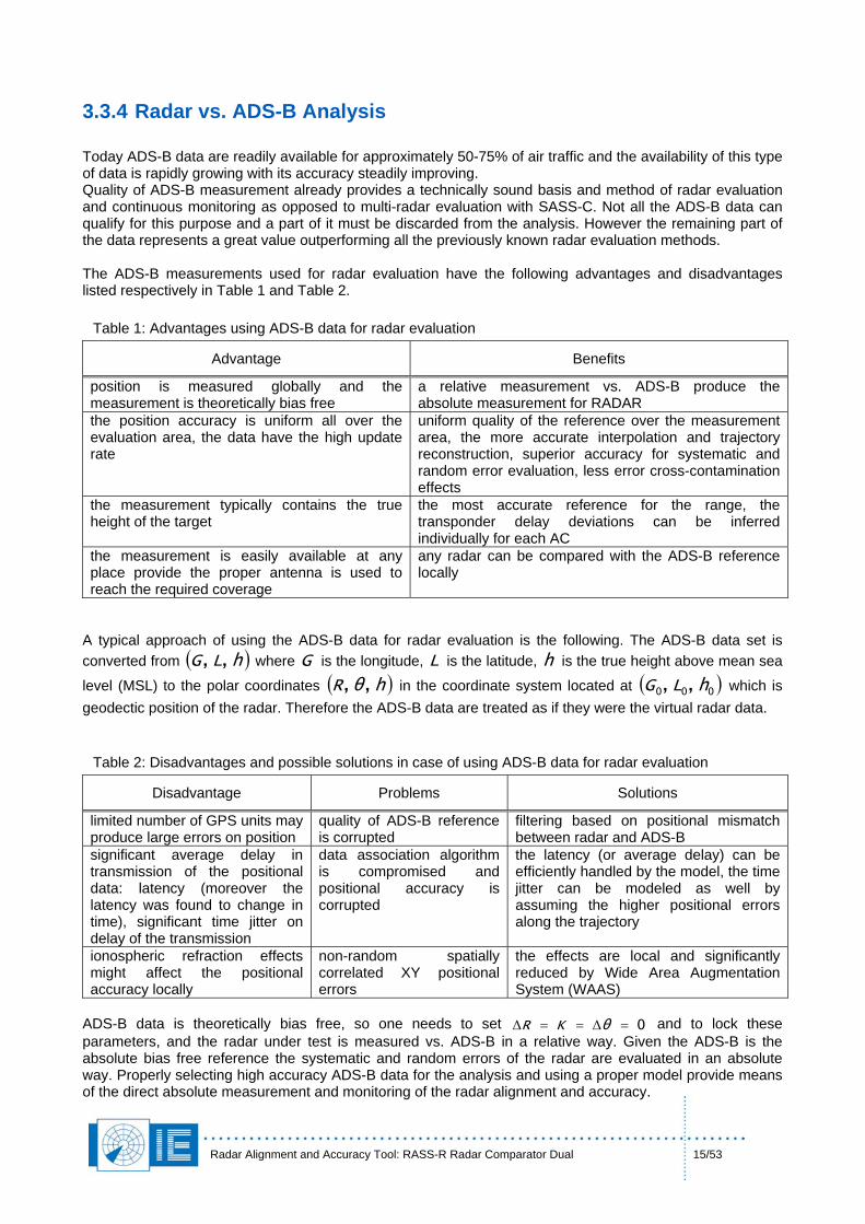
3.3.4 Radar vs. ADS-B Analysis Today ADS-B data are readily available for approximately 50-75% of air traffic and the availability of this type of data is rapidly growing with its accuracy steadily improving. Quality of ADS-B measurement already provides a technically sound basis and method of radar evaluation and continuous monitoring as opposed to multi-radar evaluation with SASS-C. Not all the ADS-B data can qualify for this purpose and a part of it must be discarded from the analysis. However the remaining part of the data represents a great value outperforming all the previously known radar evaluation methods. The ADS-B measurements used for radar evaluation have the following advantages and disadvantages listed respectively in Table 1 and Table 2.
Table 1: Advantages using ADS-B data for radar evaluation
Advantage Benefits
position is measured globally and the measurement is theoretically bias free
a relative measurement vs. ADS-B produce the absolute measurement for RADAR
the position accuracy is uniform all over the evaluation area, the data have the high update rate
uniform quality of the reference over the measurement area, the more accurate interpolation and trajectory reconstruction, superior accuracy for systematic and random error evaluation, less error cross-contamination effects
the measurement typically contains the true height of the target
the most accurate reference for the range, the transponder delay deviations can be inferred individually for each AC
the measurement is easily available at any place provide the proper antenna is used to reach the required coverage
any radar can be compared with the ADS-B reference locally
A typical approach of using the ADS-B data for radar evaluation is the following. The ADS-B data set is converted from where is the longitude, ( hLG ,, ) L is the latitude, G h is the true height above mean sea
level (MSL) to the polar coordinates in the coordinate system located at which is geodectic position of the radar. Therefore the ADS-B data are treated as if they were the virtual radar data.
( )000 ,, hLG( hθR ,, )
Table 2: Disadvantages and possible solutions in case of using ADS-B data for radar evaluation
Disadvantage Problems Solutions
limited number of GPS units may produce large errors on position
quality of ADS-B reference is corrupted
filtering based on positional mismatch between radar and ADS-B
significant average delay in transmission of the positional data: latency (moreover the latency was found to change in time), significant time jitter on delay of the transmission
data association algorithm is compromised and positional accuracy is corrupted
the latency (or average delay) can be efficiently handled by the model, the time jitter can be modeled as well by assuming the higher positional errors along the trajectory
ionospheric refraction effects might affect the positional accuracy locally
non-random spatially correlated XY positional errors
the effects are local and significantly reduced by Wide Area Augmentation System (WAAS)
ADS-B data is theoretically bias free, so one needs to set 0=== θKR ΔΔ and to lock these parameters, and the radar under test is measured vs. ADS-B in a relative way. Given the ADS-B is the absolute bias free reference the systematic and random errors of the radar are evaluated in an absolute way. Properly selecting high accuracy ADS-B data for the analysis and using a proper model provide means of the direct absolute measurement and monitoring of the radar alignment and accuracy.
Radar Alignment and Accuracy Tool: RASS-R Radar Comparator Dual 16/53
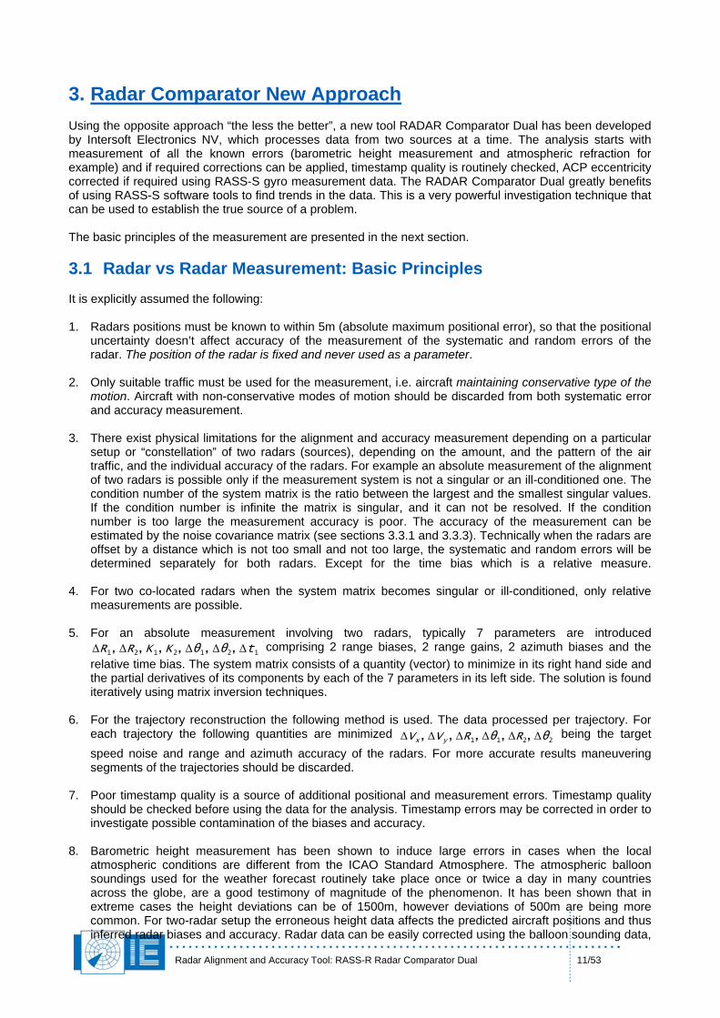
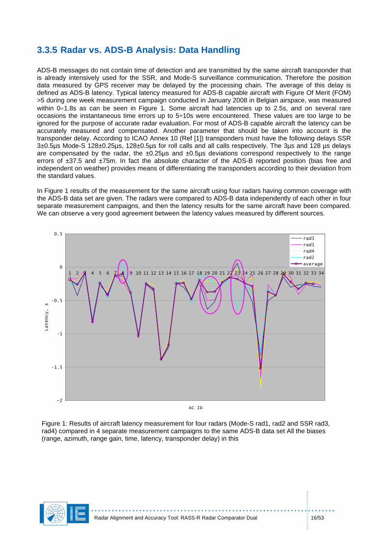
3.3.5 Radar vs. ADS-B Analysis: Data Handling ADS-B messages do not contain time of detection and are transmitted by the same aircraft transponder that is already intensively used for the SSR, and Mode-S surveillance communication. Therefore the position data measured by GPS receiver may be delayed by the processing chain. The average of this delay is defined as ADS-B latency. Typical latency measured for ADS-B capable aircraft with Figure Of Merit (FOM) >5 during one week measurement campaign conducted in January 2008 in Belgian airspace, was measured within 0÷1.8s as can be seen in Figure 1. Some aircraft had latencies up to 2.5s, and on several rare occasions the instantaneous time errors up to 5÷10s were encountered. These values are too large to be ignored for the purpose of accurate radar evaluation. For most of ADS-B capable aircraft the latency can be accurately measured and compensated. Another parameter that should be taken into account is the transponder delay. According to ICAO Annex 10 (Ref [1]) transponders must have the following delays SSR 3±0.5µs Mode-S 128±0.25µs, 128±0.5µs for roll calls and all calls respectively. The 3µs and 128 µs delays are compensated by the radar, the ±0.25µs and ±0.5µs deviations correspond respectively to the range errors of ±37.5 and ±75m. In fact the absolute character of the ADS-B reported position (bias free and independent on weather) provides means of differentiating the transponders according to their deviation from the standard values. In Figure 1 results of the measurement for the same aircraft using four radars having common coverage with the ADS-B data set are given. The radars were compared to ADS-B data independently of each other in four separate measurement campaigns, and then the latency results for the same aircraft have been compared. We can observe a very good agreement between the latency values measured by different sources.
-2
-1.5
-1
-0.5
0
0.5
1 2 3 4 5 6 7 8 9 10 11 12 13 14 15 16 17 18 19 20 21 22 23 24 25 26 27 28 29 30 31 32 33 34
AC ID
Latency, s
rad3
rad1
rad4
rad2
average
Figure 1: Results of aircraft latency measurement for four radars (Mode-S rad1, rad2 and SSR rad3, rad4) compared in 4 separate measurement campaigns to the same ADS-B data set All the biases (range, azimuth, range gain, time, latency, transponder delay) in this
Radar Alignment and Accuracy Tool: RASS-R Radar Comparator Dual 17/53
Technically instead of using system matrix containing 4 parameters we have used 2+2N parameters, i.e. , where N is the aircraft count. Since the range bias and the transponder delay errors are correlated one needs to lock the range bias. Similarly because the latency and time bias errors are correlated we need to lock the time bias. Then 2 extra parameters per each aircraft in particular the latency
i and transponder delay deviation
i further named as transponder delay are
added to the system. Optionally the range gain parameter can be measured and locked leaving 2N+1 parameters
2. The matrix solution is carried out in the standard way, please refer to
section
tθKR ΔΔΔ ,,, 222
NitRθK ii ,0,,, 22 =ΔΔΔ
tΔ
NiRt ii ,0,, =ΔΔ
RΔ
θΔ
R6.4.1 for details. The discrepancies observed for a number of aircraft can be explained as follows. In
fact ii
are independent but the errors on them may be strongly correlated, which depends mostly on the orientation of the trajectory vs. the radar. As previously accuracy of the measurement can be estimated by the noise covariance matrix calculated for each trajectory separately. In this case the matrix condition number estimator should produce an estimate of the accuracy. In practice a radial trajectory containing only inbound or only outbound section is a typical case where the ADS-B latency and the transponder delay can’t be determined separately. When a trajectory has both inbound and outbound section the separate calculation of these parameters becomes possible. Since the same aircraft trajectories have different orientation vs. different radars their latencies and transponder delays are determined with different accuracies. The latency error may also be correlated with the azimuth error however the flight patterns that create such kind of dependency are relatively rare, for example an orbital flight.
t ΔΔ ,
In order to build an estimator of the accuracy for inferred for a particular trajectory the Measurement Figure of Merit MFM is produced. For the details of the definition of this parameter please refer to section
ii Rt ΔΔ ,
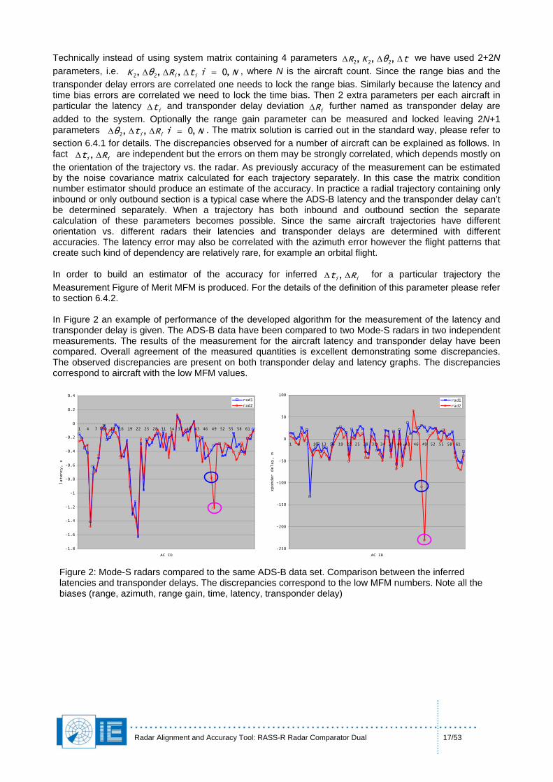
6.4.2. In Figure 2 an example of performance of the developed algorithm for the measurement of the latency and transponder delay is given. The ADS-B data have been compared to two Mode-S radars in two independent measurements. The results of the measurement for the aircraft latency and transponder delay have been compared. Overall agreement of the measured quantities is excellent demonstrating some discrepancies. The observed discrepancies are present on both transponder delay and latency graphs. The discrepancies correspond to aircraft with the low MFM values.
-1.8
-1.6
-1.4
-1.2
-1
-0.8
-0.6
-0.4
-0.2
0
0.2
0.4
1 4 7 10 13 16 19 22 25 28 31 34 37 40 43 46 49 52 55 58 61
AC ID
latency, s
rad1
rad2
-250
-200
-150
-100
-50
0
50
100
1 4 7 10 13 16 19 22 25 28 31 34 37 40 43 46 49 52 55 58 61
AC ID
xponder delay, m
rad1
rad2
Figure 2: Mode-S radars compared to the same ADS-B data set. Comparison between the inferred latencies and transponder delays. The discrepancies correspond to the low MFM numbers. Note all the biases (range, azimuth, range gain, time, latency, transponder delay)
Radar Alignment and Accuracy Tool: RASS-R Radar Comparator Dual 18/53
a) b)
c)
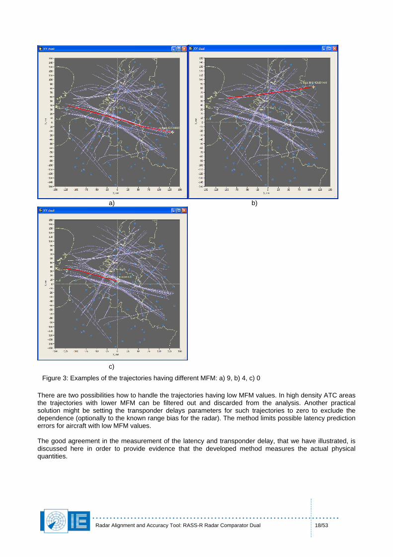
Figure 3: Examples of the trajectories having different MFM: a) 9, b) 4, c) 0 There are two possibilities how to handle the trajectories having low MFM values. In high density ATC areas the trajectories with lower MFM can be filtered out and discarded from the analysis. Another practical solution might be setting the transponder delays parameters for such trajectories to zero to exclude the dependence (optionally to the known range bias for the radar). The method limits possible latency prediction errors for aircraft with low MFM values. The good agreement in the measurement of the latency and transponder delay, that we have illustrated, is discussed here in order to provide evidence that the developed method measures the actual physical quantities.
Radar Alignment and Accuracy Tool: RASS-R Radar Comparator Dual 19/53
We need to mention that all the predicted transponder delay values are contaminated with the radar range bias. Similarly the predicted latency values contain a bias which is the UTC time bias of the radar. Timestamp quality of modern radar is excellent and typically offset by a few milliseconds from UTC. The range bias of the radar can be measured taking average over many transponders. Once the range bias as the average transponder delay is measured the individual transponder delays can be measured. To check the radar timestamp quality the best direct method is comparing it vs. GPS timestamp as a reference. Since the transponder delay characteristics are different for SSR and Mode-S interrogation modes it is logical to expect the inferred transponder delays will only match for the radars of the same type, i.e. the transponder delays inferred comparing ADS-B data with a Mode-S radar will not match the quantities determined when comparing the same ADS-B set with a SSR radar. However the inferred latency is consistent for both (as we have demonstrated in Figure 2), save for the cases when one of the radars has serious timestamp problems.
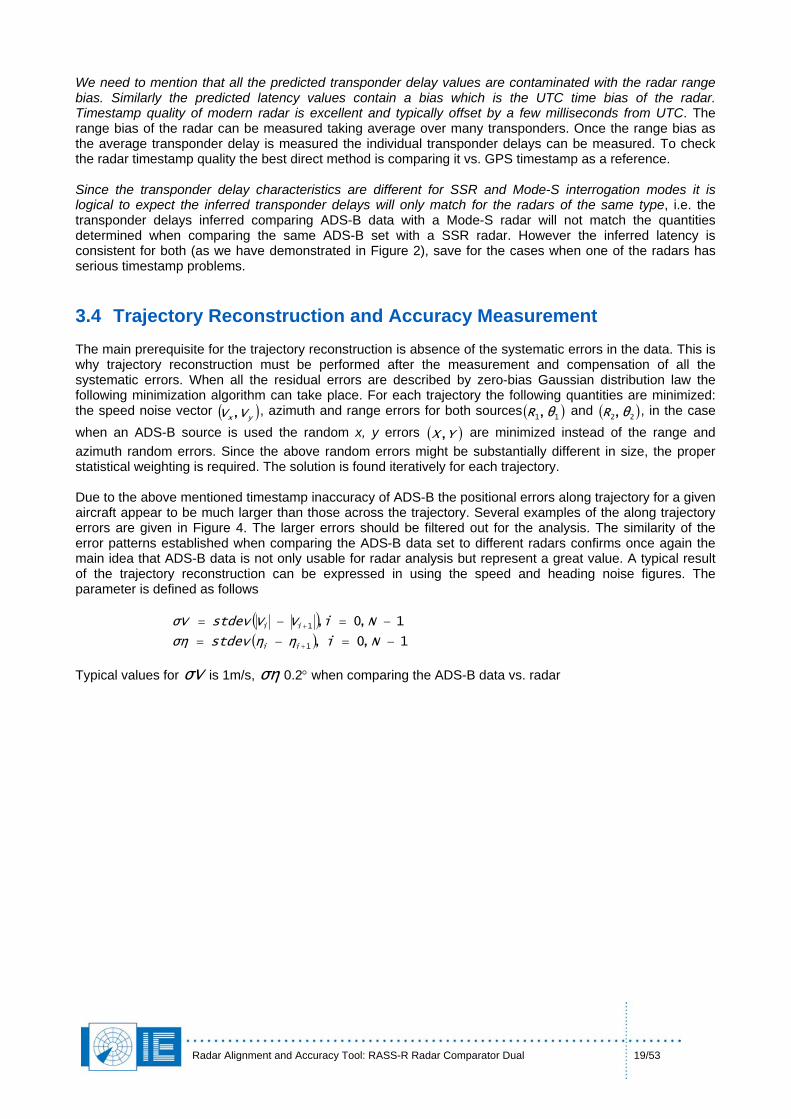
3.4 Trajectory Reconstruction and Accuracy Measurement The main prerequisite for the trajectory reconstruction is absence of the systematic errors in the data. This is why trajectory reconstruction must be performed after the measurement and compensation of all the systematic errors. When all the residual errors are described by zero-bias Gaussian distribution law the following minimization algorithm can take place. For each trajectory the following quantities are minimized: the speed noise vector ( )yx VV , , azimuth and range errors for both sources ( )11,θR and ( , in the case when an ADS-B source is used the random x, y errors
)22,θR
( )YX, are minimized instead of the range and azimuth random errors. Since the above random errors might be substantially different in size, the proper statistical weighting is required. The solution is found iteratively for each trajectory. Due to the above mentioned timestamp inaccuracy of ADS-B the positional errors along trajectory for a given aircraft appear to be much larger than those across the trajectory. Several examples of the along trajectory errors are given in Figure 4. The larger errors should be filtered out for the analysis. The similarity of the error patterns established when comparing the ADS-B data set to different radars confirms once again the main idea that ADS-B data is not only usable for radar analysis but represent a great value. A typical result of the trajectory reconstruction can be expressed in using the speed and heading noise figures. The parameter is defined as follows
( ) 1,0,1 −=−= + NiVVstdevVσ ii
( ) 1,0,1 −=−= + Niηηstdevση ii
Typical values for is 1m/s, 0.2° when comparing the ADS-B data vs. radar Vσ ση
Radar Alignment and Accuracy Tool: RASS-R Radar Comparator Dual 20/53
Figure 4: Along track ADS-B errors for 3 aircraft calculated comparing ADS-B with rad1 (white line) and then with rad2 (red line). The local differences can be accounted to the azimuth-range error cross-contamination when resampling the radar data to the ADS-B t
Radar Alignment and Accuracy Tool: RASS-R Radar Comparator Dual 21/53
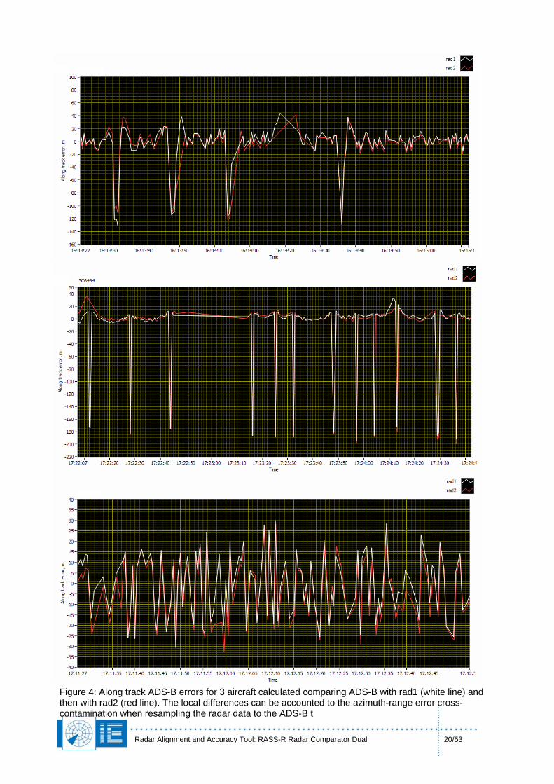
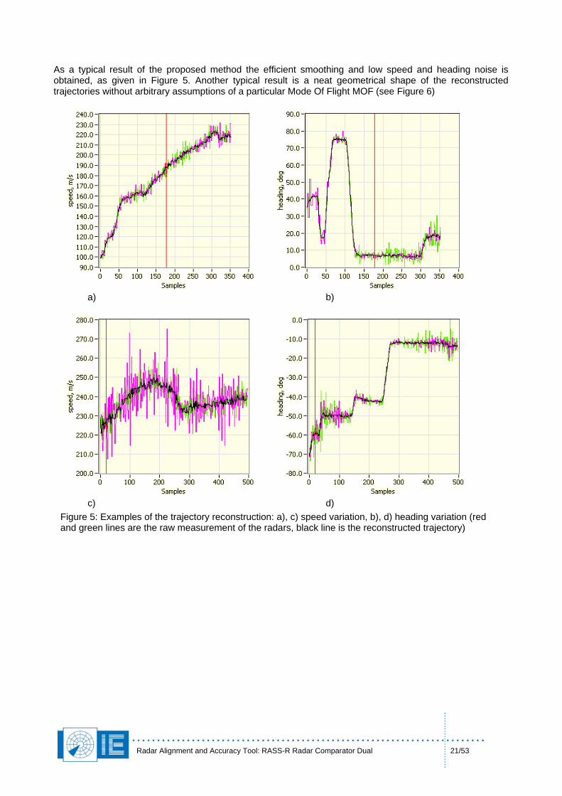
As a typical result of the proposed method the efficient smoothing and low speed and heading noise is obtained, as given in Figure 5. Another typical result is a neat geometrical shape of the reconstructed trajectories without arbitrary assumptions of a particular Mode Of Flight MOF (see Figure 6)
a) b)
c) d)
Figure 5: Examples of the trajectory reconstruction: a), c) speed variation, b), d) heading variation (red and green lines are the raw measurement of the radars, black line is the reconstructed trajectory)
Radar Alignment and Accuracy Tool: RASS-R Radar Comparator Dual 22/53
Figure 6: XY display: example of the high quality of the trajectory reconstruction
Radar Alignment and Accuracy Tool: RASS-R Radar Comparator Dual 23/53
4. Results and Applications
4.1 Case A: Real Value for Radar Evaluation and Continuous Performance Monitoring
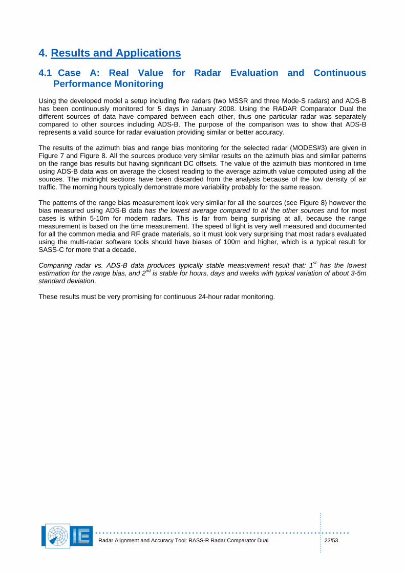
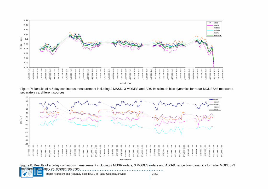
Using the developed model a setup including five radars (two MSSR and three Mode-S radars) and ADS-B has been continuously monitored for 5 days in January 2008. Using the RADAR Comparator Dual the different sources of data have compared between each other, thus one particular radar was separately compared to other sources including ADS-B. The purpose of the comparison was to show that ADS-B represents a valid source for radar evaluation providing similar or better accuracy. The results of the azimuth bias and range bias monitoring for the selected radar (MODES#3) are given in Figure 7 and Figure 8. All the sources produce very similar results on the azimuth bias and similar patterns on the range bias results but having significant DC offsets. The value of the azimuth bias monitored in time using ADS-B data was on average the closest reading to the average azimuth value computed using all the sources. The midnight sections have been discarded from the analysis because of the low density of air traffic. The morning hours typically demonstrate more variability probably for the same reason. The patterns of the range bias measurement look very similar for all the sources (see Figure 8) however the bias measured using ADS-B data has the lowest average compared to all the other sources and for most cases is within 5-10m for modern radars. This is far from being surprising at all, because the range measurement is based on the time measurement. The speed of light is very well measured and documented for all the common media and RF grade materials, so it must look very surprising that most radars evaluated using the multi-radar software tools should have biases of 100m and higher, which is a typical result for SASS-C for more that a decade. Comparing radar vs. ADS-B data produces typically stable measurement result that: 1st has the lowest estimation for the range bias, and 2nd is stable for hours, days and weeks with typical variation of about 3-5m standard deviation. These results must be very promising for continuous 24-hour radar monitoring.
Radar Alignment and Accuracy Tool: RASS-R Radar Comparator Dual 24/53
0.04
0.05
0.06
0.07
0.08
0.09
0.1
0.11
0.12
0.13
0.14
1/24/2008 4:48
1/24/2008 7:12
1/24/2008 9:36
1/24/2008 12:00
1/24/2008 14:24
1/24/2008 16:48
1/24/2008 19:12
1/24/2008 21:36
1/25/2008 0:00
1/25/2008 2:24
1/25/2008 4:48
1/25/2008 7:12
1/25/2008 9:36
1/25/2008 12:00
1/25/2008 14:24
1/25/2008 16:48
1/25/2008 19:12
1/25/2008 21:36
1/26/2008 0:00
1/26/2008 2:24
1/26/2008 4:48
1/26/2008 7:12
1/26/2008 9:36
1/26/2008 12:00
1/26/2008 14:24
1/26/2008 16:48
1/26/2008 19:12
1/26/2008 21:36
1/27/2008 0:00
1/27/2008 2:24
1/27/2008 4:48
1/27/2008 7:12
1/27/2008 9:36
1/27/2008 12:00
1/27/2008 14:24
1/27/2008 16:48
1/27/2008 19:12
1/27/2008 21:36
1/28/2008 0:00
1/28/2008 2:24
1/28/2008 4:48
1/28/2008 7:12
1/28/2008 9:36
1/28/2008 12:00
1/28/2008 14:24
1/28/2008 16:48
1/28/2008 19:12
date&time
bias, deg
adsb
mssr1
modes1
modes2
mssr2
average
Figure 7: Results of a 5-day continuous measurement including 2 MSSR, 3 MODES and ADS-B: azimuth bias dynamics for radar MODES#3 measured separately vs. different sources.
-100
-90
-80
-70
-60
-50
-40
-30
-20
-10
0
10
20
1/24/2008 4:48
1/24/2008 7:12
1/24/2008 9:36
1/24/2008 12:00
1/24/2008 14:24
1/24/2008 16:48
1/24/2008 19:12
1/24/2008 21:36
1/25/2008 0:00
1/25/2008 2:24
1/25/2008 4:48
1/25/2008 7:12
1/25/2008 9:36
1/25/2008 12:00
1/25/2008 14:24
1/25/2008 16:48
1/25/2008 19:12
1/25/2008 21:36
1/26/2008 0:00
1/26/2008 2:24
1/26/2008 4:48
1/26/2008 7:12
1/26/2008 9:36
1/26/2008 12:00
1/26/2008 14:24
1/26/2008 16:48
1/26/2008 19:12
1/26/2008 21:36
1/27/2008 0:00
1/27/2008 2:24
1/27/2008 4:48
1/27/2008 7:12
1/27/2008 9:36
1/27/2008 12:00
1/27/2008 14:24
1/27/2008 16:48
1/27/2008 19:12
1/27/2008 21:36
1/28/2008 0:00
1/28/2008 2:24
1/28/2008 4:48
1/28/2008 7:12
1/28/2008 9:36
1/28/2008 12:00
1/28/2008 14:24
1/28/2008 16:48
1/28/2008 19:12
date&time
bias, m
adsb
mssr1
modes1
modes2
mssr2
Figure 8: Results of a 5-day continuous measurement including 2 MSSR radars, 3 MODES radars and ADS-B: range bias dynamics for radar MODES#3 measured separately vs. different sources.
Radar Alignment and Accuracy Tool: RASS-R Radar Comparator Dual 25/53
)
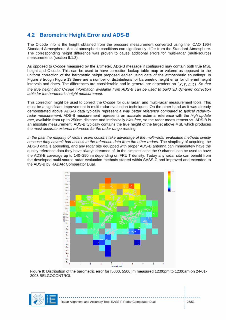
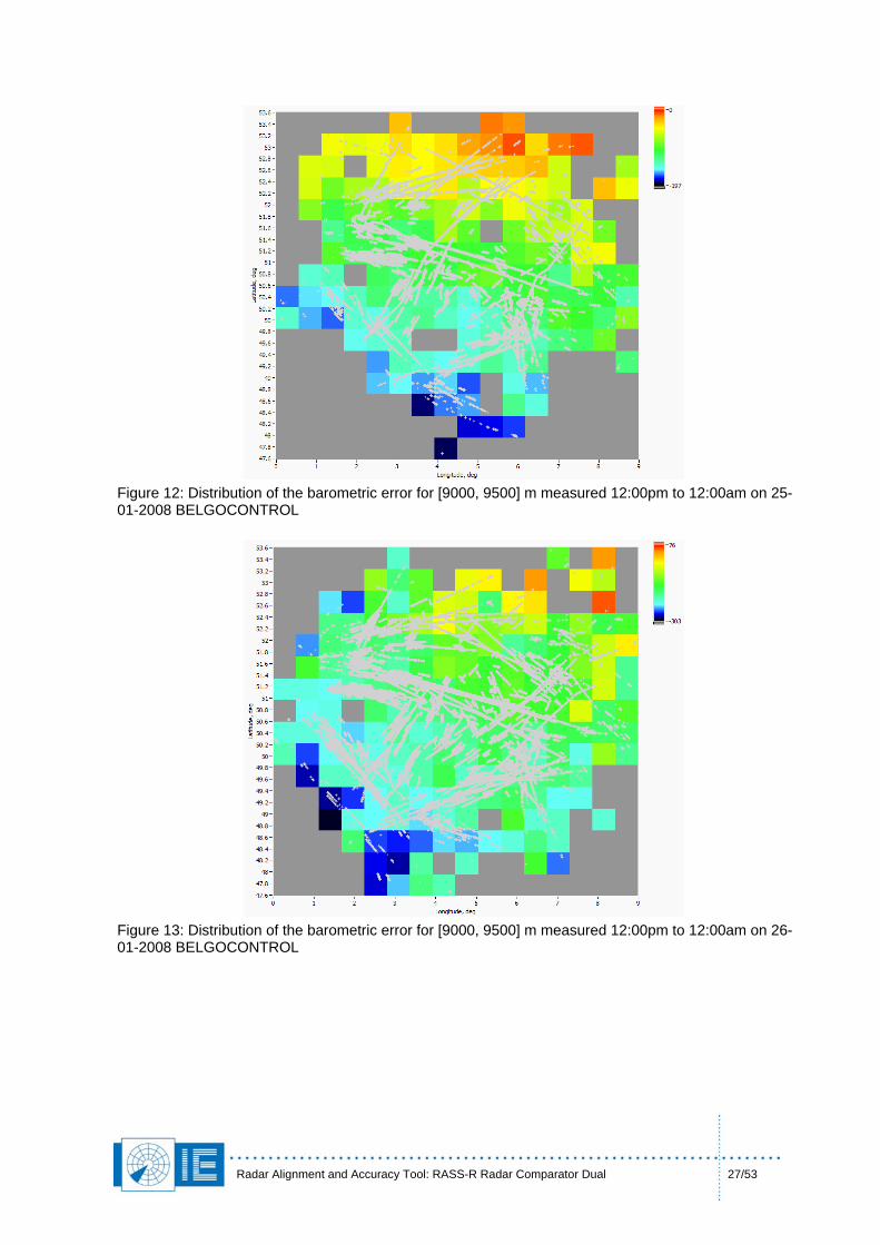
4.2 Barometric Height Error and ADS-B The C-code info is the height obtained from the pressure measurement converted using the ICAO 1964 Standard Atmosphere. Actual atmospheric conditions can significantly differ from the Standard Atmosphere. The corresponding height difference was proven to cause additional errors for multi-radar (multi-source) measurements (section 6.1.3). As opposed to C-code measured by the altimeter, ADS-B message if configured may contain both true MSL height and C-code. This can be used to have correction lookup table map or volume as opposed to the uniform correction of the barometric height proposed earlier using data of the atmospheric soundings. In Figure 9 trough Figure 13 there are a number of distributions for barometric height error for different height intervals and dates. The differences are considerable and in general are dependent on ( . So that the true height and C-code information available from ADS-B can be used to build 3D dynamic correction table for the barometric height measurement.
thYX ,,,
This correction might be used to correct the C-code for dual radar, and multi-radar measurement tools. This must be a significant improvement in multi-radar evaluation techniques. On the other hand as it was already demonstrated above ADS-B data typically represent a way better reference compared to typical radar-to-radar measurement. ADS-B measurement represents an accurate external reference with the high update rate, available from up to 250nm distance and intrinsically bias-free, so the radar measurement vs. ADS-B is an absolute measurement. ADS-B typically contains the true height of the target above MSL which produces the most accurate external reference for the radar range reading. In the past the majority of radars users couldn’t take advantage of the multi-radar evaluation methods simply because they haven’t had access to the reference data from the other radars. The simplicity of acquiring the ADS-B data is appealing, and any radar site equipped with proper ADS-B antenna can immediately have the quality reference data they have always dreamed of. In the simplest case the Ω channel can be used to have the ADS-B coverage up to 140÷250nm depending on FRUIT density. Today any radar site can benefit from the developed multi-source radar evaluation methods started within SASS-C and improved and extended to the ADS-B by RADAR Comparator Dual.
Figure 9: Distribution of the barometric error for [5000, 5500] m measured 12:00pm to 12:00am on 24-01-2008 BELGOCONTROL
Radar Alignment and Accuracy Tool: RASS-R Radar Comparator Dual 26/53
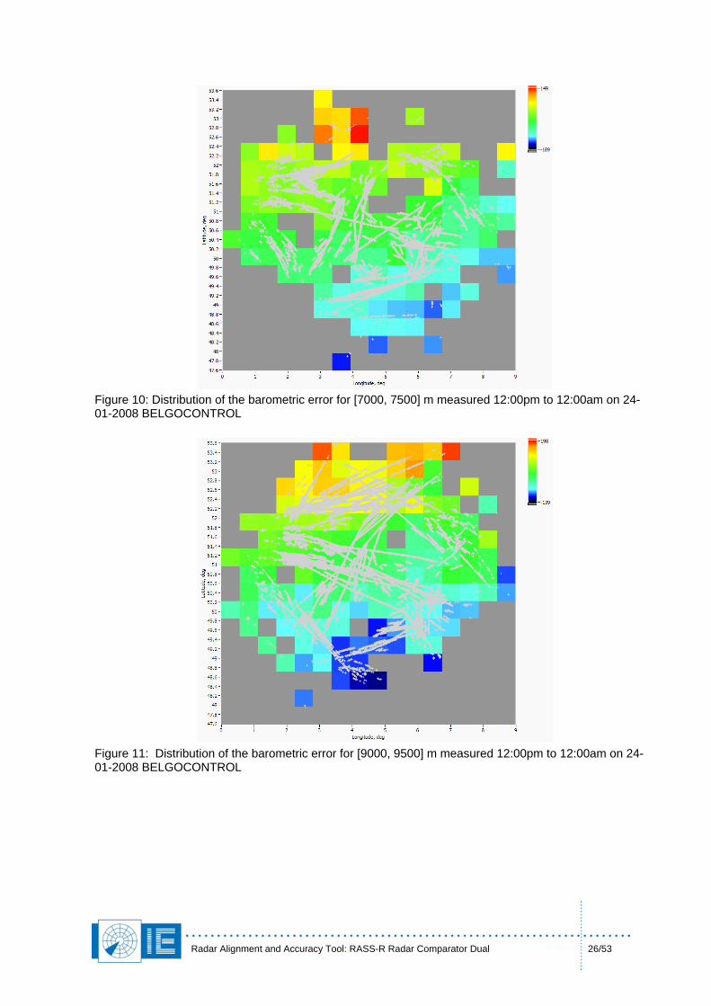
Figure 10: Distribution of the barometric error for [7000, 7500] m measured 12:00pm to 12:00am on 24-01-2008 BELGOCONTROL
Figure 11: Distribution of the barometric error for [9000, 9500] m measured 12:00pm to 12:00am on 24-01-2008 BELGOCONTROL
Radar Alignment and Accuracy Tool: RASS-R Radar Comparator Dual 27/53
Figure 12: Distribution of the barometric error for [9000, 9500] m measured 12:00pm to 12:00am on 25-01-2008 BELGOCONTROL
Figure 13: Distribution of the barometric error for [9000, 9500] m measured 12:00pm to 12:00am on 26-01-2008 BELGOCONTROL
Radar Alignment and Accuracy Tool: RASS-R Radar Comparator Dual 28/53
4.3 Case B: Radar Radome Influence Evaluation and Monopulse Distortion Correction
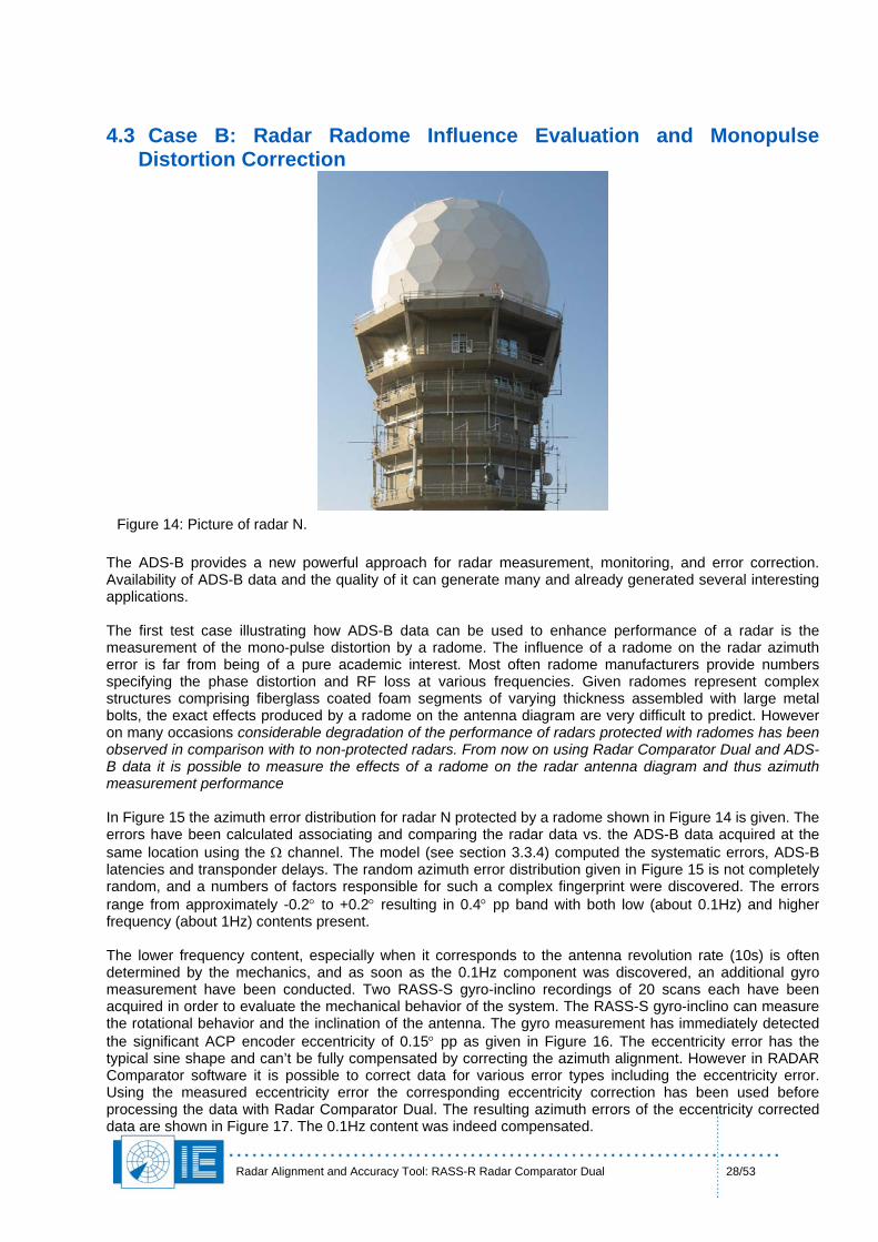
Figure 14: Picture of radar N.
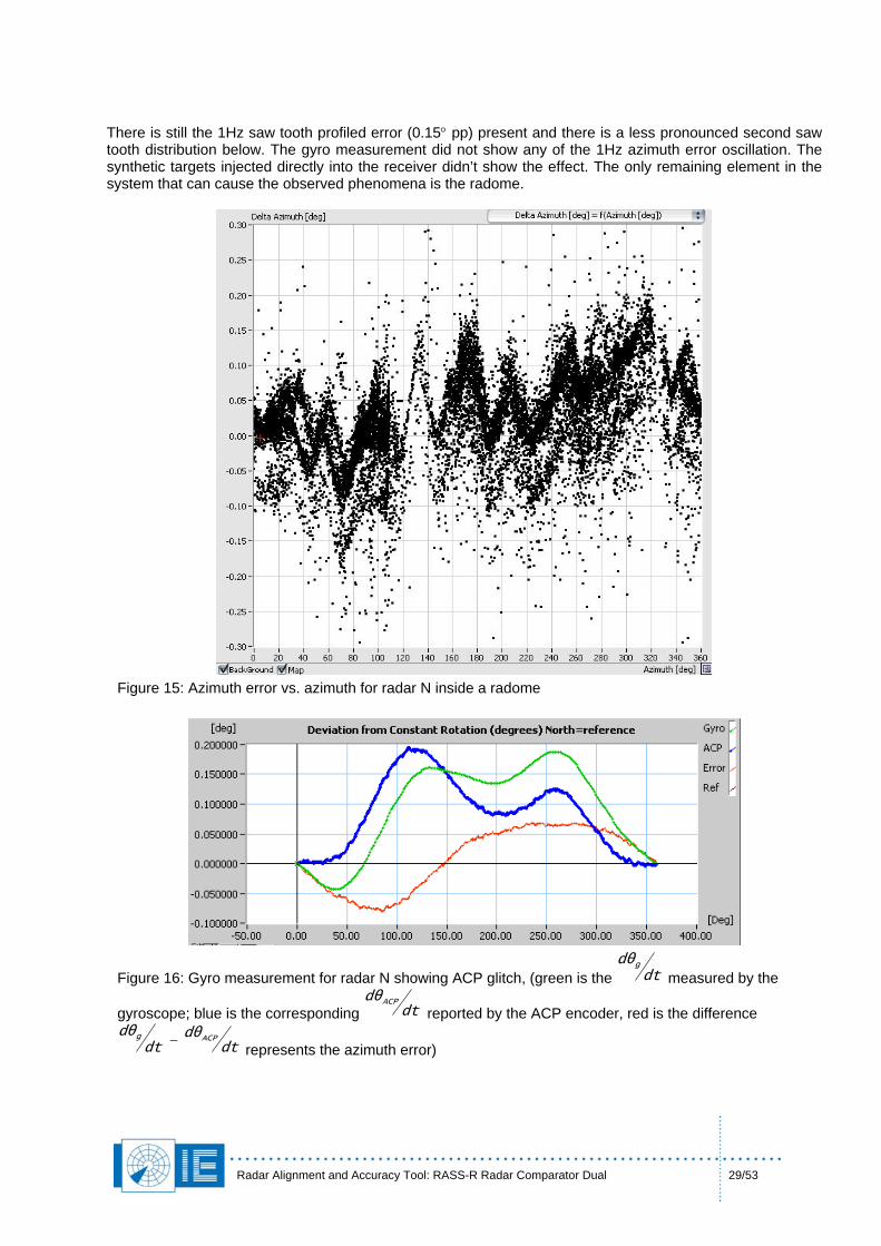
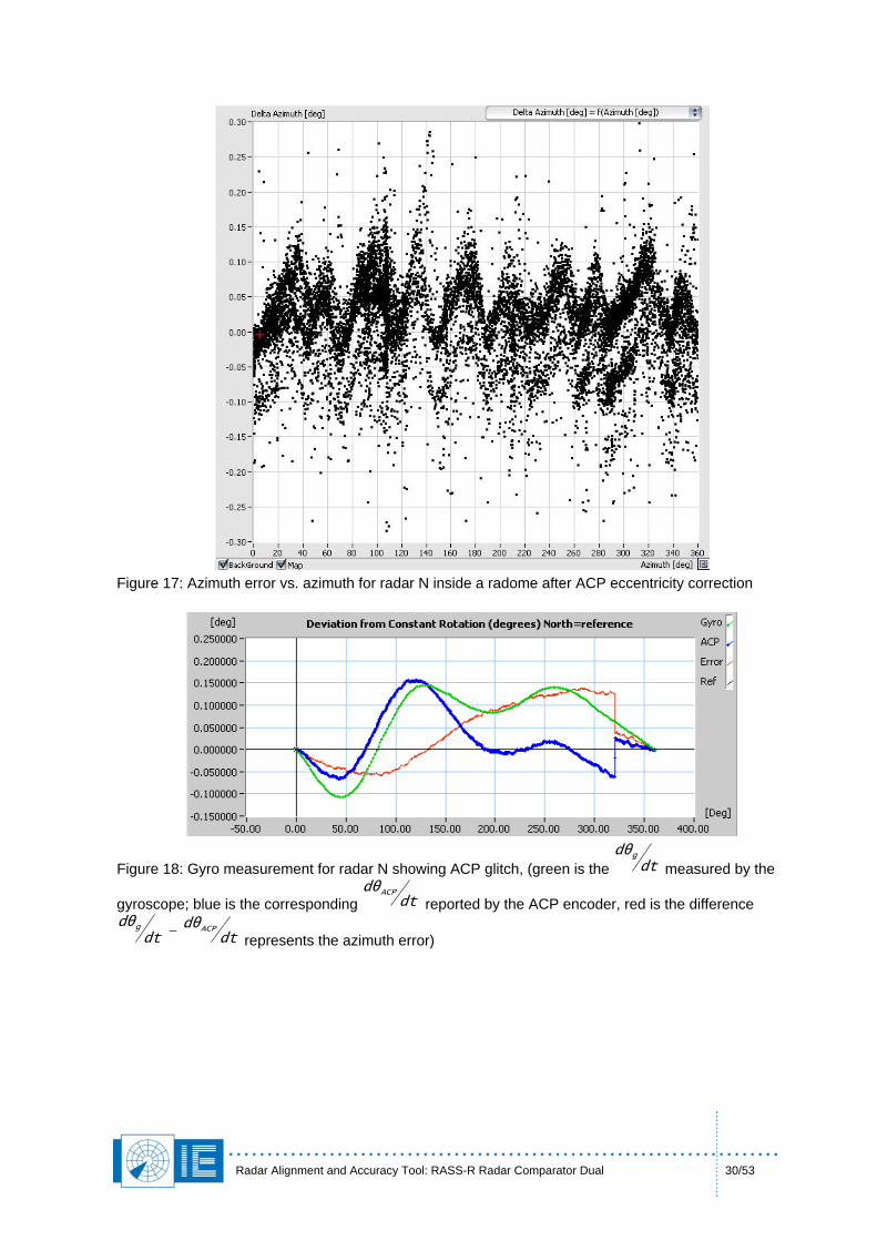
The ADS-B provides a new powerful approach for radar measurement, monitoring, and error correction. Availability of ADS-B data and the quality of it can generate many and already generated several interesting applications. The first test case illustrating how ADS-B data can be used to enhance performance of a radar is the measurement of the mono-pulse distortion by a radome. The influence of a radome on the radar azimuth error is far from being of a pure academic interest. Most often radome manufacturers provide numbers specifying the phase distortion and RF loss at various frequencies. Given radomes represent complex structures comprising fiberglass coated foam segments of varying thickness assembled with large metal bolts, the exact effects produced by a radome on the antenna diagram are very difficult to predict. However on many occasions considerable degradation of the performance of radars protected with radomes has been observed in comparison with to non-protected radars. From now on using Radar Comparator Dual and ADS-B data it is possible to measure the effects of a radome on the radar antenna diagram and thus azimuth measurement performance In Figure 15 the azimuth error distribution for radar N protected by a radome shown in Figure 14 is given. The errors have been calculated associating and comparing the radar data vs. the ADS-B data acquired at the same location using the Ω channel. The model (see section 3.3.4) computed the systematic errors, ADS-B latencies and transponder delays. The random azimuth error distribution given in Figure 15 is not completely random, and a numbers of factors responsible for such a complex fingerprint were discovered. The errors range from approximately -0.2° to +0.2° resulting in 0.4° pp band with both low (about 0.1Hz) and higher frequency (about 1Hz) contents present. The lower frequency content, especially when it corresponds to the antenna revolution rate (10s) is often determined by the mechanics, and as soon as the 0.1Hz component was discovered, an additional gyro measurement have been conducted. Two RASS-S gyro-inclino recordings of 20 scans each have been acquired in order to evaluate the mechanical behavior of the system. The RASS-S gyro-inclino can measure the rotational behavior and the inclination of the antenna. The gyro measurement has immediately detected the significant ACP encoder eccentricity of 0.15° pp as given in Figure 16. The eccentricity error has the typical sine shape and can’t be fully compensated by correcting the azimuth alignment. However in RADAR Comparator software it is possible to correct data for various error types including the eccentricity error. Using the measured eccentricity error the corresponding eccentricity correction has been used before processing the data with Radar Comparator Dual. The resulting azimuth errors of the eccentricity corrected data are shown in Figure 17. The 0.1Hz content was indeed compensated.
Radar Alignment and Accuracy Tool: RASS-R Radar Comparator Dual 29/53
There is still the 1Hz saw tooth profiled error (0.15° pp) present and there is a less pronounced second saw tooth distribution below. The gyro measurement did not show any of the 1Hz azimuth error oscillation. The synthetic targets injected directly into the receiver didn’t show the effect. The only remaining element in the system that can cause the observed phenomena is the radome.
Figure 15: Azimuth error vs. azimuth for radar N inside a radome
Figure 16: Gyro measurement for radar N showing ACP glitch, (green is the dtθd g
measured by the
gyroscope; blue is the corresponding dtθd ACP
reported by the ACP encoder, red is the difference
dtθd
dtθd
ACPg − represents the azimuth error)
Radar Alignment and Accuracy Tool: RASS-R Radar Comparator Dual 30/53
Figure 17: Azimuth error vs. azimuth for radar N inside a radome after ACP eccentricity correction
Figure 18: Gyro measurement for radar N showing ACP glitch, (green is the dtθd g
measured by the
gyroscope; blue is the corresponding dtθd ACP
reported by the ACP encoder, red is the difference
dtθd
dtθd
ACPg − represents the azimuth error)
Radar Alignment and Accuracy Tool: RASS-R Radar Comparator Dual 31/53
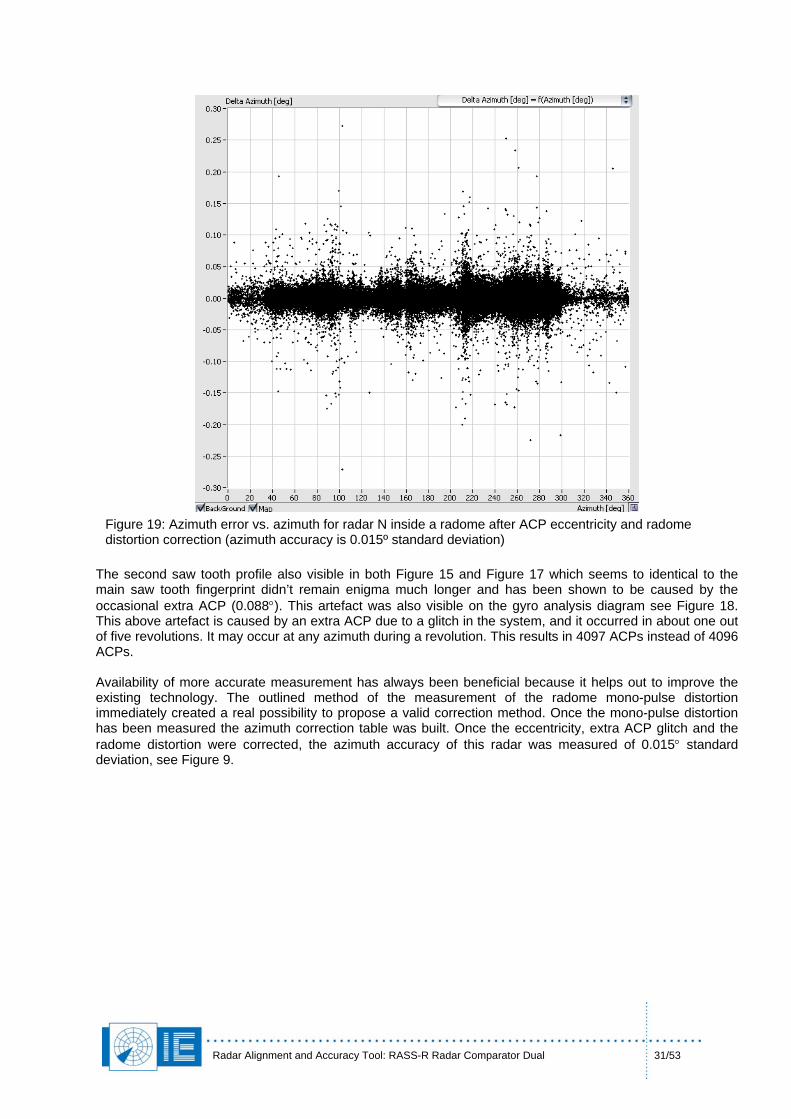
Figure 19: Azimuth error vs. azimuth for radar N inside a radome after ACP eccentricity and radome distortion correction (azimuth accuracy is 0.015º standard deviation)
The second saw tooth profile also visible in both Figure 15 and Figure 17 which seems to identical to the main saw tooth fingerprint didn’t remain enigma much longer and has been shown to be caused by the occasional extra ACP (0.088°). This artefact was also visible on the gyro analysis diagram see Figure 18. This above artefact is caused by an extra ACP due to a glitch in the system, and it occurred in about one out of five revolutions. It may occur at any azimuth during a revolution. This results in 4097 ACPs instead of 4096 ACPs. Availability of more accurate measurement has always been beneficial because it helps out to improve the existing technology. The outlined method of the measurement of the radome mono-pulse distortion immediately created a real possibility to propose a valid correction method. Once the mono-pulse distortion has been measured the azimuth correction table was built. Once the eccentricity, extra ACP glitch and the radome distortion were corrected, the azimuth accuracy of this radar was measured of 0.015° standard deviation, see Figure 9.
Radar Alignment and Accuracy Tool: RASS-R Radar Comparator Dual 32/53
4.4 Case C: Measurement of the Azimuth Errors Generated by Lightening Poles
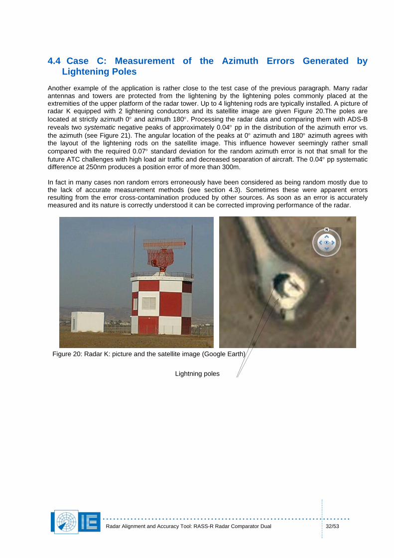
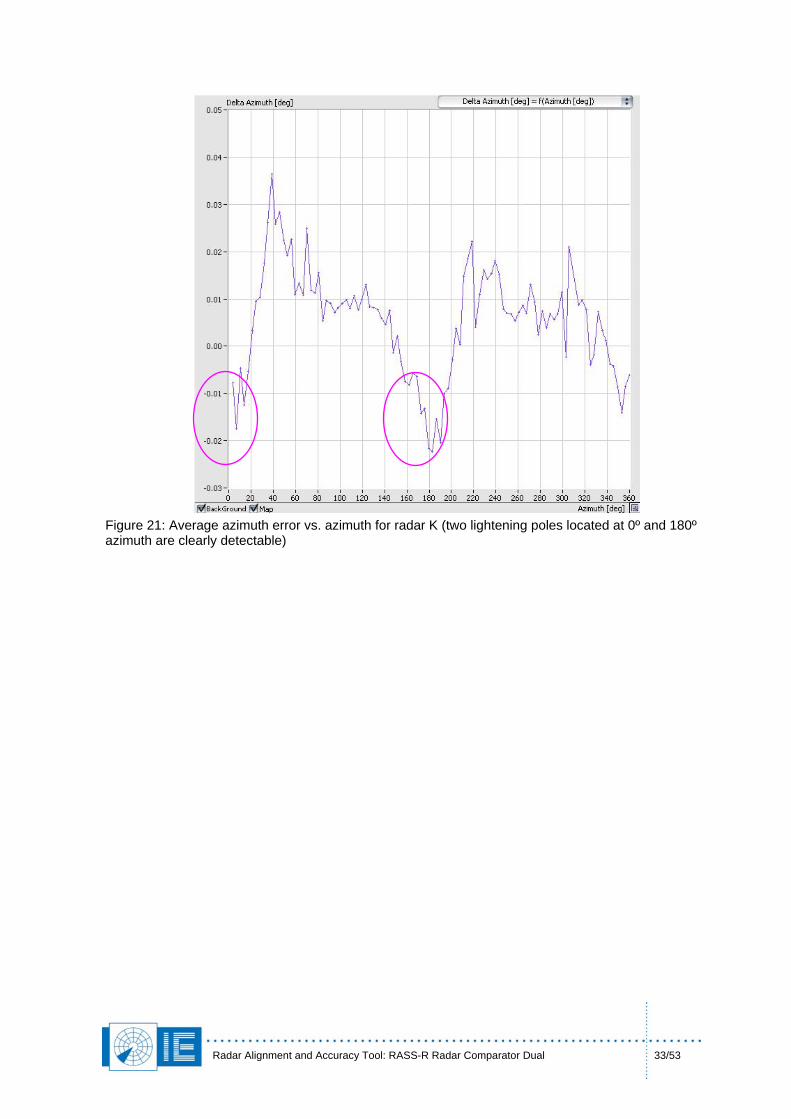
Another example of the application is rather close to the test case of the previous paragraph. Many radar antennas and towers are protected from the lightening by the lightening poles commonly placed at the extremities of the upper platform of the radar tower. Up to 4 lightening rods are typically installed. A picture of radar K equipped with 2 lightening conductors and its satellite image are given Figure 20.The poles are located at strictly azimuth 0° and azimuth 180°. Processing the radar data and comparing them with ADS-B reveals two systematic negative peaks of approximately 0.04° pp in the distribution of the azimuth error vs. the azimuth (see Figure 21). The angular location of the peaks at 0° azimuth and 180° azimuth agrees with the layout of the lightening rods on the satellite image. This influence however seemingly rather small compared with the required 0.07° standard deviation for the random azimuth error is not that small for the future ATC challenges with high load air traffic and decreased separation of aircraft. The 0.04° pp systematic difference at 250nm produces a position error of more than 300m. In fact in many cases non random errors erroneously have been considered as being random mostly due to the lack of accurate measurement methods (see section 4.3). Sometimes these were apparent errors resulting from the error cross-contamination produced by other sources. As soon as an error is accurately measured and its nature is correctly understood it can be corrected improving performance of the radar.
Figure 20: Radar K: picture and the satellite image (Google Earth)
Lightning poles
Radar Alignment and Accuracy Tool: RASS-R Radar Comparator Dual 33/53
Figure 21: Average azimuth error vs. azimuth for radar K (two lightening poles located at 0º and 180º azimuth are clearly detectable)
Radar Alignment and Accuracy Tool: RASS-R Radar Comparator Dual 34/53
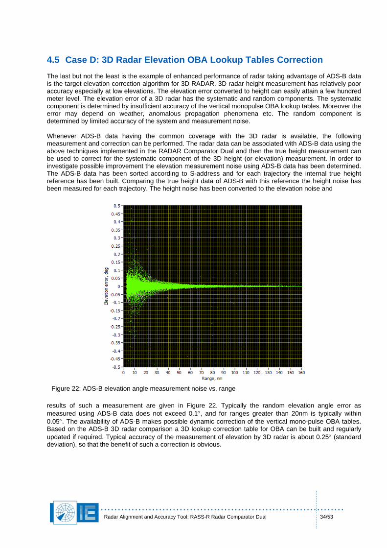
4.5 Case D: 3D Radar Elevation OBA Lookup Tables Correction The last but not the least is the example of enhanced performance of radar taking advantage of ADS-B data is the target elevation correction algorithm for 3D RADAR. 3D radar height measurement has relatively poor accuracy especially at low elevations. The elevation error converted to height can easily attain a few hundred meter level. The elevation error of a 3D radar has the systematic and random components. The systematic component is determined by insufficient accuracy of the vertical monopulse OBA lookup tables. Moreover the error may depend on weather, anomalous propagation phenomena etc. The random component is determined by limited accuracy of the system and measurement noise. Whenever ADS-B data having the common coverage with the 3D radar is available, the following measurement and correction can be performed. The radar data can be associated with ADS-B data using the above techniques implemented in the RADAR Comparator Dual and then the true height measurement can be used to correct for the systematic component of the 3D height (or elevation) measurement. In order to investigate possible improvement the elevation measurement noise using ADS-B data has been determined. The ADS-B data has been sorted according to S-address and for each trajectory the internal true height reference has been built. Comparing the true height data of ADS-B with this reference the height noise has been measured for each trajectory. The height noise has been converted to the elevation noise and
Figure 22: ADS-B elevation angle measurement noise vs. range
results of such a measurement are given in Figure 22. Typically the random elevation angle error as measured using ADS-B data does not exceed 0.1°, and for ranges greater than 20nm is typically within 0.05°. The availability of ADS-B makes possible dynamic correction of the vertical mono-pulse OBA tables. Based on the ADS-B 3D radar comparison a 3D lookup correction table for OBA can be built and regularly updated if required. Typical accuracy of the measurement of elevation by 3D radar is about 0.25° (standard deviation), so that the benefit of such a correction is obvious.
Radar Alignment and Accuracy Tool: RASS-R Radar Comparator Dual 35/53
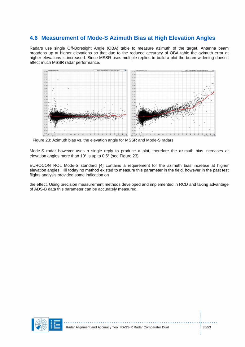
4.6 Measurement of Mode-S Azimuth Bias at High Elevation Angles Radars use single Off-Boresight Angle (OBA) table to measure azimuth of the target. Antenna beam broadens up at higher elevations so that due to the reduced accuracy of OBA table the azimuth error at higher elevations is increased. Since MSSR uses multiple replies to build a plot the beam widening doesn’t affect much MSSR radar performance.
Figure 23: Azimuth bias vs. the elevation angle for MSSR and Mode-S radars
Mode-S radar however uses a single reply to produce a plot, therefore the azimuth bias increases at elevation angles more than 10° is up to 0.5° (see Figure 23) EUROCONTROL Mode-S standard [4] contains a requirement for the azimuth bias increase at higher elevation angles. Till today no method existed to measure this parameter in the field, however in the past test flights analysis provided some indication on the effect. Using precision measurement methods developed and implemented in RCD and taking advantage of ADS-B data this parameter can be accurately measured.
Radar Alignment and Accuracy Tool: RASS-R Radar Comparator Dual 36/53
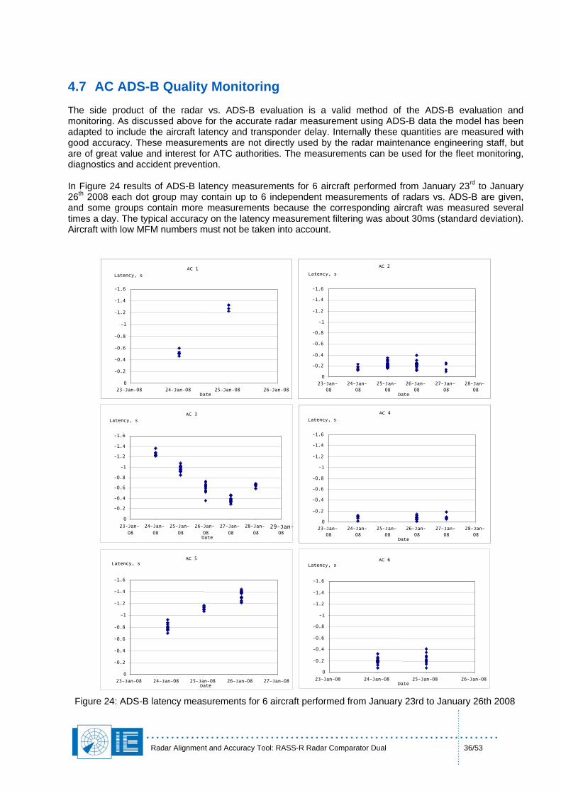
4.7 AC ADS-B Quality Monitoring The side product of the radar vs. ADS-B evaluation is a valid method of the ADS-B evaluation and monitoring. As discussed above for the accurate radar measurement using ADS-B data the model has been adapted to include the aircraft latency and transponder delay. Internally these quantities are measured with good accuracy. These measurements are not directly used by the radar maintenance engineering staff, but are of great value and interest for ATC authorities. The measurements can be used for the fleet monitoring, diagnostics and accident prevention. In Figure 24 results of ADS-B latency measurements for 6 aircraft performed from January 23rd to January 26th 2008 each dot group may contain up to 6 independent measurements of radars vs. ADS-B are given, and some groups contain more measurements because the corresponding aircraft was measured several times a day. The typical accuracy on the latency measurement filtering was about 30ms (standard deviation). Aircraft with low MFM numbers must not be taken into account.
Figure 24: ADS-B latency measurements for 6 aircraft performed from January 23rd to January 26th 2008
-1.6
-1.4
-1.2
-1
-0.8
-0.6
-0.4
-0.2
0
23-Jan-08 24-Jan-08 25-Jan-08 26-Jan-08Date
Latency, sAC 6
-1.6 -1.4 -1.2
-1
-0.8 -0.6 -0.4 -0.2
0 23-Jan-08 24-Jan-08 25-Jan-08
Date 26-Jan-08 27-Jan-08
Latency, s AC 5
-1.6
-1.4
-1.2
-1
-0.8
-0.6
-0.4
-0.2
0
23-Jan-
08
24-Jan-
08
25-Jan-
08
26-Ja - n
08 27-Ja - n
08 28-Jan-
08Date
Latency, s
AC 4
-1.6
-1.4
-1.2
-1
-0.8
-0.6
-0.4
-0.2
0 23-Jan-
08 24-Jan-
08 25-Jan-
08
26-Jan- 08
27-Jan-
08
28-Jan-
08
29-Jan-08
Date
Latency, s AC 3
-1.6
-1.4
-1.2
-1
-0.8
-0.6
-0.4
-0.2
0
23-Jan-
08
24-Jan-
08
25-Jan-
08
26-Jan- 08
27-Ja - n
08 28-Jan-
08Date
Latency, s
AC 2
-1.6 -1.4 -1.2
-1 -0.8 -0.6 -0.4 -0.2
0 23-Jan-08 24-Jan-08 25-Jan-08 26-Jan-08
Date
Latency, s AC 1
Radar Alignment and Accuracy Tool: RASS-R Radar Comparator Dual 37/53
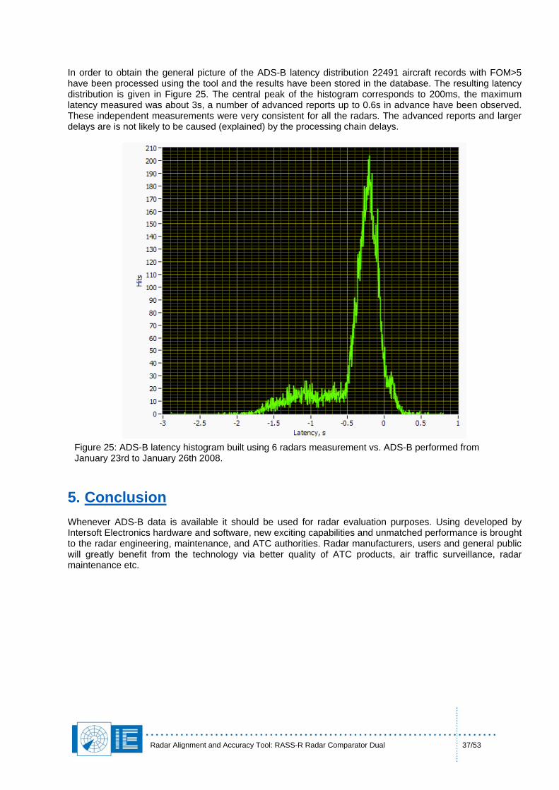
In order to obtain the general picture of the ADS-B latency distribution 22491 aircraft records with FOM>5 have been processed using the tool and the results have been stored in the database. The resulting latency distribution is given in Figure 25. The central peak of the histogram corresponds to 200ms, the maximum latency measured was about 3s, a number of advanced reports up to 0.6s in advance have been observed. These independent measurements were very consistent for all the radars. The advanced reports and larger delays are is not likely to be caused (explained) by the processing chain delays.
Figure 25: ADS-B latency histogram built using 6 radars measurement vs. ADS-B performed from January 23rd to January 26th 2008.
5. Conclusion Whenever ADS-B data is available it should be used for radar evaluation purposes. Using developed by Intersoft Electronics hardware and software, new exciting capabilities and unmatched performance is brought to the radar engineering, maintenance, and ATC authorities. Radar manufacturers, users and general public will greatly benefit from the technology via better quality of ATC products, air traffic surveillance, radar maintenance etc.
Radar Alignment and Accuracy Tool: RASS-R Radar Comparator Dual 38/53
6. Annex 1: Radar Comparator Dual Used Methods
6.1 Data Correction Methods
6.1.1 Timestamp Analysis Before any data fusion process combining data originating from sensors of different type the timestamp accuracy must be inspected. The correct timing is as important as the correct position for the accurate positional reconstruction and the correct object association. First, the integrity of timestamps for plot (track) data, the sector messages and the north messages are tested. Number of scans and the average time per scan is determined for all three sources. If the data are consistent, sector messages timing is used to produce the best linear fit using a number of the antenna rotations (default setting). Using the obtained linear fit the timestamps of the plot data are evaluated and corrected if required. If the time of detection is available the correction of the timestamp is not required. On the older radars when only the time of recording is available, the correction may have some benefits, especially when using multi-source comparison techniques. With high load air traffic situations the time of recording may have up 1-1.5 s error vs. the correct time of detection. However the user must be aware of the some unwanted effects this correction might cause. For example if the radar has significant eccentricity, correcting for the timestamp error will actually increase the effect of the eccentricity, moving the timestamp in the direction of the eccentricity.
6.1.2 ACP Eccentricity Correction ACP encoder eccentricity was shown to have significant negative impact on the results of a multi-radar or dual radar evaluation. The same radar with eccentric encoder may typically have 0.03-0.04° azimuth bias difference when measured to radars that happen to have the common coverage at the opposite maxima of the eccentricity sine wave. The phenomenon becomes more complex when more than one radar from the evaluation setup has this problem. Moreover the azimuth biases of the other radars compared to the radar with ACP eccentricity may appear different compared to the other pairs. The eccentricity is the systematic error so it must be corrected before the measurement.
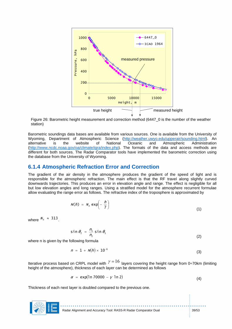
6.1.3 Barometric Height Correction using Atmospheric Soundings The C-code info is the height obtained from the pressure measurement converted using the ICAO 1964 Standard Atmosphere. It is known that actual atmospheric conditions can significantly differ from the Standard Atmosphere. This difference was proven to cause additional errors for multi-radar measurements. As given in Figure 26 the C-code (height) is converted to the actual pressure according to ICAO Standard Atmosphere, and then the actual height is obtained using the local pressure vs. height curve provided from the atmospheric sounding measurement. Unfortunately the assumption of the uniformity of the barometric pressure distribution (both in 3D and time) is not correct but until recently the distributed barometric measurement was not available. ADS-B data typically contain true height of the target above MSL and C-code. This can be used to have correction table map or volume as opposed to the uniform correction of the barometric height.
Radar Alignment and Accuracy Tool: RASS-R Radar Comparator Dual 39/53
0
200
400
600
800
1000
0 5000 10000 15000
Height, m
Pressure, hPa
6447_0
ICAO 1964
measured pressure
measured height true height
Figure 26: Barometric height measurement and correction method (6447_0 is the number of the weather station)
Barometric soundings data bases are available from various sources. One is available from the University of Wyoming, Department of Atmospheric Science (http://weather.uwyo.edu/upperair/sounding.html). An alternative is the website of National Oceanic and Atmospheric Administration (http://www.ncdc.noaa.gov/oa/climate/igra/index.php). The formats of the data and access methods are different for both sources. The Radar Comparator tools have implemented the barometric correction using the database from the University of Wyoming.
6.1.4 Atmospheric Refraction Error and Correction The gradient of the air density in the atmosphere produces the gradient of the speed of light and is responsible for the atmospheric refraction. The main effect is that the RF travel along slightly curved downwards trajectories. This produces an error in elevation angle and range. The effect is negligible for all but low elevation angles and long ranges. Using a stratified model for the atmosphere recurrent formulae allow evaluating the range error as follows. The refractive index of the troposphere is approximated by
⎟⎠⎞
⎜⎝⎛−=
7exp)(
hNhN S
(1) where . 313≈SN
1
2
12 sinsin θ
n
nθ =
(2) where n is given by the following formula (3) ( ) 6101 −×+= hNn
16=γIterative process based on CRPL model with layers covering the height range from 0÷70km (limiting
height of the atmosphere), thickness of each layer can be determined as follows
( 2ln70000lnexp γα )−= (4) Thickness of each next layer is doubled compared to the previous one.
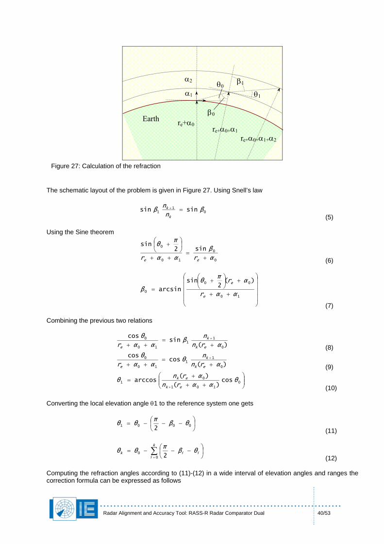
Radar Alignment and Accuracy Tool: RASS-R Radar Comparator Dual 40/53
α1
α2 θ0 θ1
β0
β1
re+α0 re+α0+α1
re+α0+α1+α2
Earth
Figure 27: Calculation of the refraction
The schematic layout of the problem is given in Figure 27. Using Snell’s law
01
1 sinsin βn
nβ
k
k =+
(5) Using the Sine theorem
0
0
10
0 sin2sin
αr
β
ααr
πθ
ee +=
++
⎟⎠⎞
⎜⎝⎛ +
(6)
⎟⎟⎟⎟
⎠
⎞
⎜⎜⎜⎜
⎝
⎛
++
+⎟⎠⎞
⎜⎝⎛ +
=10
00
0
)(2
sin
arcsinααr
αrπ
θ
βe
e
(7) Combining the previous two relations
)(sin
cos
0
11
10
0
αrn
nβ
ααr
θ
ek
k
e +=
+++
(8)
)(cos
cos
0
11
10
0
αrn
nθ
ααr
θ
ek
k
e +=
+++
(9)
⎟⎟⎠
⎞⎜⎜⎝
⎛++
+=
+0
101
01 cos
)(
)(arccos θ
ααrn
αrnθ
ek
ek
(10) Converting the local elevation angle θ1 to the reference system one gets
⎟⎠⎞
⎜⎝⎛ −−−= 00012
θβπ
θθ (11)
∑=
⎟⎠⎞
⎜⎝⎛ −−−=
k
iiik θβ
πθθ
00
2 (12) Computing the refraction angles according to (11)-(12) in a wide interval of elevation angles and ranges the correction formula can be expressed as follows
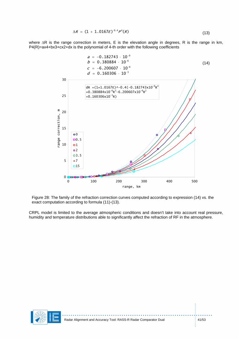
Radar Alignment and Accuracy Tool: RASS-R Radar Comparator Dual 41/53
(13) )()0167.11( 44.0 RPER −+=Δ where ΔR is the range correction in meters, E is the elevation angle in degrees, R is the range in km, P4(R)=ax4+bx3+cx2+dx is the polynomial of 4-th order with the following coefficients
910182743.0 −⋅−=a−
(14) 610380884.0 ⋅=b
610200607.6 −⋅−=c
310160306.0 −⋅=d
dR =(1+1.0167E)^-0.4(-0.182743x10⁻⁹R4
+0.380884x10⁻⁶R3-6.200607x10
-6R2
+0.160306x10⁻³R)
0
5
10
15
20
25
30
0 100 200 300 400 500
range, km
range correction, m
0
0.5
1
2
3.5
7
15
Figure 28: The family of the refraction correction curves computed according to expression (14) vs. the exact computation according to formula (11)-(13).
CRPL model is limited to the average atmospheric conditions and doesn’t take into account real pressure, humidity and temperature distributions able to significantly affect the refraction of RF in the atmosphere.
Radar Alignment and Accuracy Tool: RASS-R Radar Comparator Dual 42/53
6.2 General Radar Data Processing Methods
6.2.1 XYZ-t Filtering Method The filtered position of the plot given measurements ( )22' tX ( ) 3,1,' =itX ii
taken is given by the following formula
( ) ( ) ( )( ) 2
13
23112322
3
1
3
2' X
tt
ttXttXtX +⎟⎟
⎠
⎞⎜⎜⎝
⎛−
−+−=
(15) where represent vectors. The above smoothing method is efficient for linear motion and generates significant positional errors with manoeuvring aircraft (with the error magnitude strongly depending on the data update rate and the angular velocity).
321 , X, XX
6.2.2 Linear Interpolation To re-sample the radar data to bring the plots to the same time, the following formula is used
( ) ( ) ( )13
12
1213 tt
tt
XXXtX −
−−
+=, (16)
. where
231 ttt ≤≤
Radar Alignment and Accuracy Tool: RASS-R Radar Comparator Dual 43/53
6.2.3 Correlation of the Data An efficient and fast method to correlate data taken from two sources can be based on 3/A-code or S-address. The data produced by each source are sorted first using their codes and then their timestamps. The data sets having the same code originated from both radars are processed by a correlation algorithm. As a result a number of tracks which belong to both sources are established. Sources of different nature generally represent more effort for the association process, for example analysing PSR vs. SSR (PSR vs. MODES, ADS-B vs. SSR etc.). In those cases the method relies on target position, time and dynamics. Given possible misalignment errors including timestamp errors, especially for ADS-B that can be significant, this algorithm is subject to various difficulties, with large errors tending to deteriorate quality of the correlation result.
6.2.4 Height Reconstruction For established tracks simultaneously monitored by two sources the height reconstruction is performed. In this case one has to make sure that the height information is of the same type. The purpose of this filtering is to reconstruct the correct height of the aircraft in presence of garbled or absence of C-code info. Incorrect height information may produce significant positional errors when converting the coordinates from the local coordinate systems to the reference system.
6.3 Radar vs. Radar Analysis
6.3.1 Systematic Errors Measurement The dual radar comparison is typically used in order to determine the systematic errors of the both sources (radars or ADS-B). The systematic errors for radars include range bias, range gain, azimuth bias and time bias. The systematic errors for ADS-B may include latencies and individual transponder delay variations. The measurement algorithm assumes that all the measured parameters are described by the Gaussian normal distribution law. The first two moments mean value and the standard deviation are of practical interest. Here below those two are named as biases (or systematic errors) and accuracy (or random errors) respectively. Depending on the constellation and nature of the data various minimization algorithms are used.
Radar Alignment and Accuracy Tool: RASS-R Radar Comparator Dual 44/53
6.3.2 Matrix Structure Seven parameters are introduced for two radars as the systematic errors that include 2 range biases, 2 range gains, 2 azimuth biases and a relative time bias. For each pair of the plots taken at the same time t the following function is to be minimized
1212121 ,,,,,, tθθKKRR ΔΔΔΔΔ
),,(),,,(),,,,,,( 2222111111212121 θKRXtθKRXtθθKKRRD ΔΔΔΔΔΔΔΔΔΔ −= (17)
where D is the distance between the plots,
12 are respectively range biases,
gains, azimuth biases and the relative time bias of the radars, are the coordinates of the plots. As a particular case only components will be used. If the measurement noise is zero, the exact solution
2121 may be obtained with the sufficient number of equations to uniquely
resolve all the parameters. In presence of the measurement noise the problem is solved iteratively using the following method. Function (6) is represented in the shape
12121 ,,,,,, tθθKKRR ΔΔΔΔΔ
21, XX
YX,
,1θ ΔΔ 0),,,,,( 12 =tθKKRRD ΔΔΔ
...
),,,,,,(),,,,,,(
1
1
2
2
1
1
2
2
1
1
2
2
1
1
102010201020101212121
+∂∂
+∂∂
+∂∂
+∂∂
+∂∂
+∂∂
+∂∂
+
+=
tt
Dθ
θ
Dθ
θ
DK
K
DK
K
DR
R
DR
R
D
tθθKKRRDtθθKKRRD
ΔΔΔΔΔΔΔ
ΔΔΔΔΔΔΔΔΔΔ
(18) where are some initial approximations for the measured values. In our case we take the initial value for the actual measured distance between the plots as
10201020102010 ,,,,,, tθθKKRR ΔΔΔΔΔ,( 10RD Δ
KKRRD
),,,,, 102010201020 tθθKKR ΔΔΔΔdtθθ =),, 102010 ΔΔΔ . To minimize (18) we must require ,,,,( 20102010 ΔΔ
0),,,,,,( 1212121 =+ dtθθKKRRD ΔΔΔΔΔ (19)
Relation (20) can be linearized as follows
dtt
Dθ
θ
Dθ
θ
DK
K
DK
K
DR
R
DR
R
D−=
∂∂
+∂∂
+∂∂
+∂∂
+∂∂
+∂∂
+∂∂
1
1
2
2
1
1
2
2
1
1
2
2
1
1
ΔΔΔΔΔΔΔ (20)
Equations of this type written down for each pair of the plots will result in the following system
⎥⎥⎥⎥⎥⎥⎥⎥⎥⎥⎥⎥
⎦
⎤
⎢⎢⎢⎢⎢⎢⎢⎢⎢⎢⎢⎢
⎣
⎡
−=
⎥⎥⎥⎥⎥⎥⎥⎥⎥
⎦
⎤
⎢⎢⎢⎢⎢⎢⎢⎢⎢
⎣
⎡
Δ
Δ
Δ
ΔΔΔΔ
⎥⎥⎥⎥⎥⎥⎥⎥⎥⎥⎥⎥
⎦
⎤
⎢⎢⎢⎢⎢⎢⎢⎢⎢⎢⎢⎢
⎣
⎡
∂∂
∂∂∂∂∂∂
∂∂
∂∂∂∂∂∂
∂∂
∂∂∂∂∂∂
∂∂
∂∂
∂∂
∂∂
∂∂
∂∂
∂∂
∂∂
∂∂
∂∂
∂∂
∂∂
∂∂
∂∂
∂∂
∂∂
n
nnnnnnn
d
d
d
d
d
d
t
K
K
R
R
t
D
t
Dt
Dt
D
D
D
D
D
D
D
D
D
K
D
K
D
R
D
R
D
K
D
K
D
R
D
R
DK
D
K
D
R
D
R
DK
D
K
D
R
D
R
D
5
4
3
2
1
1
2
1
2
1
2
1
1
1
3
1
2
1
1
2
2
3
2
2
2
1
1
1
3
1
2
1
1
2121
2
3
1
3
2
3
1
3
2
2
1
2
2
2
1
2
2
1
1
1
2
1
1
1
...
...
θθ
θ
θ
θ
θ
θ
θ
θ
θ
(21) or in matrix notations
DAX = (22)
Radar Alignment and Accuracy Tool: RASS-R Radar Comparator Dual 45/53
where the matrix [A] has n×7 size, the unknown vector X has 7×1 size, the right hand term D is n×1 vector. System (22) has n×7 size n>7 and is called over-determined. The solution is sought using the following method
DAAXA TT = (23)
BAXAT = (24)
AATDAB T= is 7×1 vector, and where is a 7×7 matrix which can be decomposed in upper-triangular and lower-triangular matrices as follows (Cholesky decomposition)
(25) CCAA TT = Then the solution is found as follows separately solving two systems
(26) BYCT = and then (27) YCX = Solving equations (26) and (27) the vector-update [ ]1212121 tKKRR ΔΔΔΔΔΔΔ θθ is obtained, the initial values of the biases are updated and the process is cycled iteratively till the required minimum size of the update is reached. If the right hand side vector is a random vector, then the approximate solution has the following covariance matrix
(28) 12 )()( −= CCx Tσ
The partial derivatives composing matrix A are calculated as follows.
13
1
22
2
11
1
22
2
11
1
22
2
11
1
)cos(
)cos(
)cos(
)cos(
)cos(
)cos(
)cos(
Vt
D
RD
RD
RK
D
RK
D
KR
D
KR
D
i
i
i
i
i
i
i
α
αθ
αθ
ϕ
ϕ
ϕ
ϕ
=∂∂
=∂∂
=∂∂
=∂∂
=∂∂
=∂∂
=∂∂
(29)
32121 ,,,, αααϕwhere the corresponding quantities ϕ are shown in Figure 29.
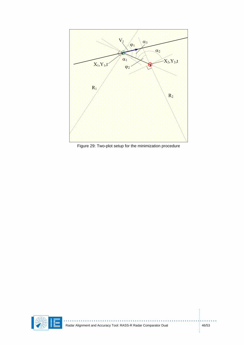
Radar Alignment and Accuracy Tool: RASS-R Radar Comparator Dual 46/53
R1 R2
X1,Y1,t X2,Y2,t
V1
ϕ2
α2 ϕ1
α1
α3
Figure 29: Two-plot setup for the minimization procedure
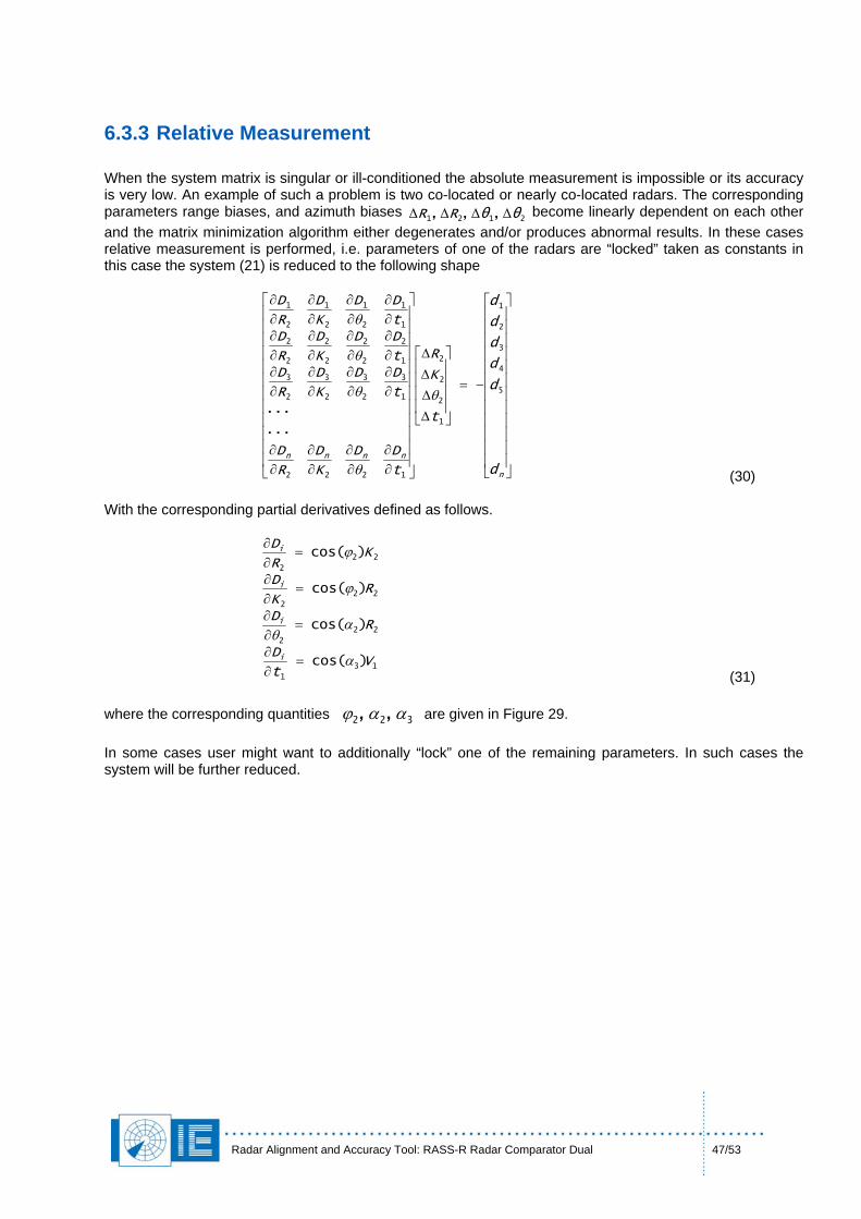
Radar Alignment and Accuracy Tool: RASS-R Radar Comparator Dual 47/53
6.3.3 Relative Measurement When the system matrix is singular or ill-conditioned the absolute measurement is impossible or its accuracy is very low. An example of such a problem is two co-located or nearly co-located radars. The corresponding parameters range biases, and azimuth biases become linearly dependent on each other and the matrix minimization algorithm either degenerates and/or produces abnormal results. In these cases relative measurement is performed, i.e. parameters of one of the radars are “locked” taken as constants in this case the system (21) is reduced to the following shape
2121 ,,, θθRR ΔΔΔΔ
⎥⎥⎥⎥⎥⎥⎥⎥⎥⎥⎥⎥
⎦
⎤
⎢⎢⎢⎢⎢⎢⎢⎢⎢⎢⎢⎢
⎣
⎡
−=
⎥⎥⎥⎥
⎦
⎤
⎢⎢⎢⎢
⎣
⎡
ΔΔΔΔ
⎥⎥⎥⎥⎥⎥⎥⎥⎥⎥⎥⎥
⎦
⎤
⎢⎢⎢⎢⎢⎢⎢⎢⎢⎢⎢⎢
⎣
⎡
∂∂
∂∂
∂∂
∂∂
∂∂
∂∂
∂∂
∂∂
∂∂
∂∂
∂∂
∂∂
∂∂
∂∂
∂∂
∂∂
n
nnnn
d
d
d
d
d
d
t
K
R
t
DD
K
D
R
D
t
DD
K
D
R
Dt
DD
K
D
R
Dt
DD
K
D
R
D
5
4
3
2
1
1
2
2
2
1222
1
3
2
3
2
3
2
3
1
2
2
2
2
2
2
2
1
1
2
1
2
1
2
1
...
...θ
θ
θ
θ
θ
(30) With the corresponding partial derivatives defined as follows.
13
1
22
2
22
2
22
2
)cos(
)cos(
)cos(
)cos(
Vt
D
RD
RK
D
KR
D
i
i
i
i
α
αθ
ϕ
ϕ
=∂∂
=∂∂
=∂∂
=∂∂
(31)
322 ,, ααϕ are given in Figure 29. where the corresponding quantities In some cases user might want to additionally “lock” one of the remaining parameters. In such cases the system will be further reduced.
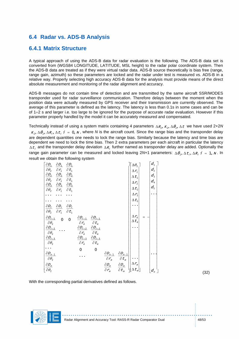
Radar Alignment and Accuracy Tool: RASS-R Radar Comparator Dual 48/53
6.4 Radar vs. ADS-B Analysis
6.4.1 Matrix Structure A typical approach of using the ADS-B data for radar evaluation is the following. The ADS-B data set is converted from (WGS84 LONGITUDE, LATITUDE, MSL height) to the radar polar coordinate system. Then the ADS-B data are treated as if they were virtual radar data. ADS-B source theoretically is bias free (range, range gain, azimuth) so these parameters are locked and the radar under test is measured vs. ADS-B in a relative way. Properly selecting high accuracy ADS-B data for the analysis must provide means of the direct absolute measurement and monitoring of the radar alignment and accuracy. ADS-B messages do not contain time of detection and are transmitted by the same aircraft SSR/MODES transponder used for radar surveillance communication. Therefore delays between the moment when the position data were actually measured by GPS receiver and their transmission are currently observed. The average of this parameter is defined as the latency. The latency is less than 0.1s in some cases and can be of 1÷2 s and larger i.e. too large to be ignored for the purpose of accurate radar evaluation. However if this parameter properly handled by the model it can be accurately measured and compensated. Technically instead of using a system matrix containing 4 parameters we have used 2+2N
, where N is the aircraft count. Since the range bias and the transponder delay are dependent quantities one needs to lock the range bias. Similarly because the latency and time bias are dependent we need to lock the time bias. Then 2 extra parameters per each aircraft in particular the latency
i and the transponder delay deviation
i further named as transponder delay are added. Optionally the
range gain parameter can be measured and locked leaving 2N+1 parameters:
tθKR ΔΔΔ ,,, 222
θ ,2
NitRθK ii ,0,,, 22 =ΔΔΔ
tΔ RΔNiRt ii ,1, =ΔΔΔ . In
result we obtain the following system
⎥⎥⎥⎥⎥⎥⎥⎥⎥⎥⎥⎥⎥⎥⎥⎥⎥⎥⎥⎥⎥⎥⎥⎥⎥⎥⎥⎥
⎦
⎤
⎢⎢⎢⎢⎢⎢⎢⎢⎢⎢⎢⎢⎢⎢⎢⎢⎢⎢⎢⎢⎢⎢⎢⎢⎢⎢⎢⎢
⎣
⎡
−=
⎥⎥⎥⎥⎥⎥⎥⎥⎥⎥⎥⎥⎥⎥⎥⎥⎥⎥⎥⎥⎥⎥⎥⎥⎥⎥⎥⎥
⎦
⎤
⎢⎢⎢⎢⎢⎢⎢⎢⎢⎢⎢⎢⎢⎢⎢⎢⎢⎢⎢⎢⎢⎢⎢⎢⎢⎢⎢⎢
⎣
⎡
ΔΔ
ΔΔ
ΔΔΔ
ΔΔΔΔ
⎥⎥⎥⎥⎥⎥⎥⎥⎥⎥⎥⎥⎥⎥⎥⎥⎥⎥⎥⎥⎥⎥⎥⎥⎥⎥⎥⎥
⎦
⎤
⎢⎢⎢⎢⎢⎢⎢⎢⎢⎢⎢⎢⎢⎢⎢⎢⎢⎢⎢⎢⎢⎢⎢⎢⎢⎢⎢⎢
⎣
⎡
∂∂
∂∂
∂∂
∂∂
∂∂
∂∂
∂∂
∂∂
∂∂
∂∂
∂∂
∂∂
∂∂∂∂∂∂
∂∂
∂∂
∂∂
∂∂
∂∂
∂∂
∂∂
∂∂
∂∂
∂∂
∂∂
∂∂
−−
++
++
++
−
+
+
+
nm
m
k
k
m
n
m
n
m
n
m
n
k
i
k
i
k
i
k
i
k
i
k
i
n
n
i
i
i
iii
d
d
d
d
d
d
t
r
tr
t
r
t
r
t
r
t
D
t
D
r
D
r
D
t
D
r
Dt
D
r
Dt
D
r
D
D
D
D
D
D
t
D
r
DD
t
D
r
DDt
D
r
DDt
D
r
DD
...
...
...
...
...
0
...
0...
...
00
...
...
...
...
...
...
5
4
3
2
1
3
3
2
2
1
1
2
11
33
22
11
2
2
1
2
3
2
2
2
1
112
1
3
1
3
2
3
1
2
1
2
2
2
1
1
1
1
2
1 θ
θ
θ
θ
θ
θ
θ
θ
θ
θ
(32) With the corresponding partial derivatives defined as follows.
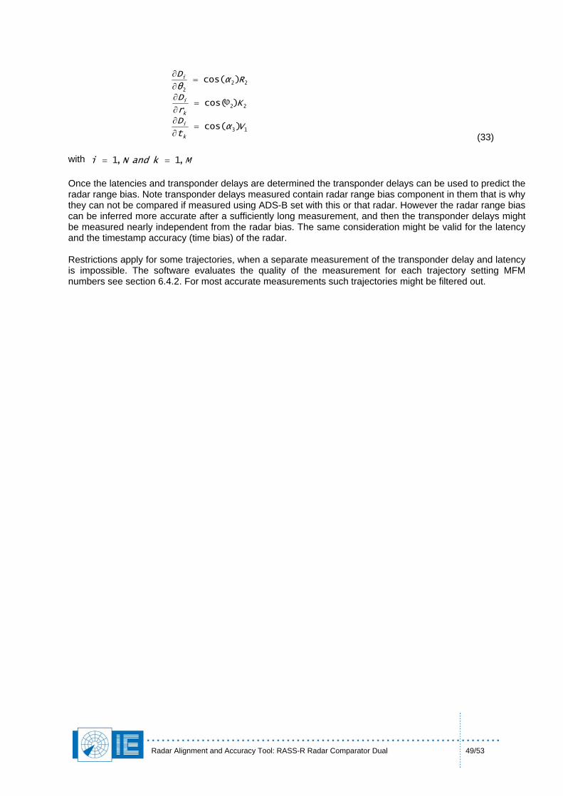
Radar Alignment and Accuracy Tool: RASS-R Radar Comparator Dual 49/53
13
22
22
2
)cos(
)cos(
)cos(
Vαt
D
Kr
D
Rαθ
D
k
i
k
i
i
=∂∂
=∂∂
=∂∂
ϕ
(33) with MkandNi ,1,1 == Once the latencies and transponder delays are determined the transponder delays can be used to predict the radar range bias. Note transponder delays measured contain radar range bias component in them that is why they can not be compared if measured using ADS-B set with this or that radar. However the radar range bias can be inferred more accurate after a sufficiently long measurement, and then the transponder delays might be measured nearly independent from the radar bias. The same consideration might be valid for the latency and the timestamp accuracy (time bias) of the radar. Restrictions apply for some trajectories, when a separate measurement of the transponder delay and latency is impossible. The software evaluates the quality of the measurement for each trajectory setting MFM numbers see section 6.4.2. For most accurate measurements such trajectories might be filtered out.
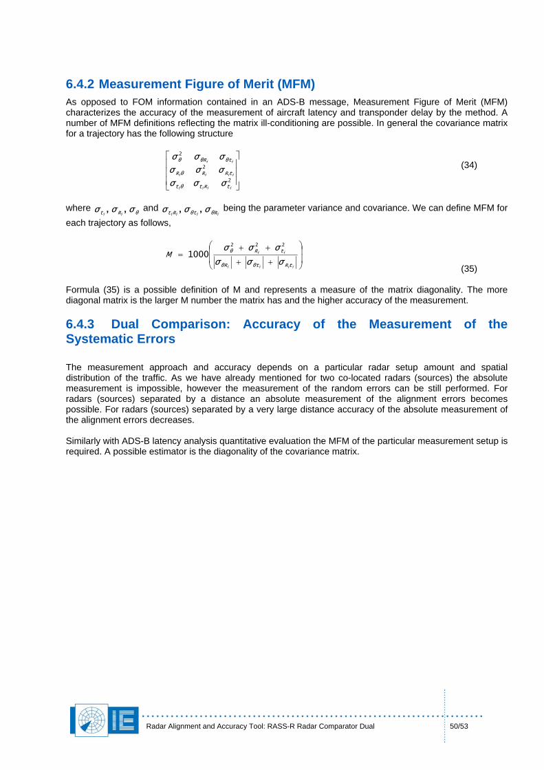
Radar Alignment and Accuracy Tool: RASS-R Radar Comparator Dual 50/53
6.4.2 Measurement Figure of Merit (MFM) As opposed to FOM information contained in an ADS-B message, Measurement Figure of Merit (MFM) characterizes the accuracy of the measurement of aircraft latency and transponder delay by the method. A number of MFM definitions reflecting the matrix ill-conditioning are possible. In general the covariance matrix for a trajectory has the following structure
(34)
⎥⎥⎥
⎦
⎤
⎢⎢⎢
⎣
⎡
2
2
2
iiii
iiii
ii
tRtθt
tRRθR
tθRθθ
σσσ
σσσ
σσσ
where and being the parameter variance and covariance. We can define MFM for each trajectory as follows,
θRt σσσii,,
iiii RθtθRt σσσ ,,
⎟⎟
⎠
⎞
⎜⎜
⎝
⎛
++
++=
iiii
ii
tRtθRθ
tRθ
σσσ
σσσM
222
1000
(35) Formula (35) is a possible definition of M and represents a measure of the matrix diagonality. The more diagonal matrix is the larger M number the matrix has and the higher accuracy of the measurement.
6.4.3 Dual Comparison: Accuracy of the Measurement of the Systematic Errors The measurement approach and accuracy depends on a particular radar setup amount and spatial distribution of the traffic. As we have already mentioned for two co-located radars (sources) the absolute measurement is impossible, however the measurement of the random errors can be still performed. For radars (sources) separated by a distance an absolute measurement of the alignment errors becomes possible. For radars (sources) separated by a very large distance accuracy of the absolute measurement of the alignment errors decreases. Similarly with ADS-B latency analysis quantitative evaluation the MFM of the particular measurement setup is required. A possible estimator is the diagonality of the covariance matrix.
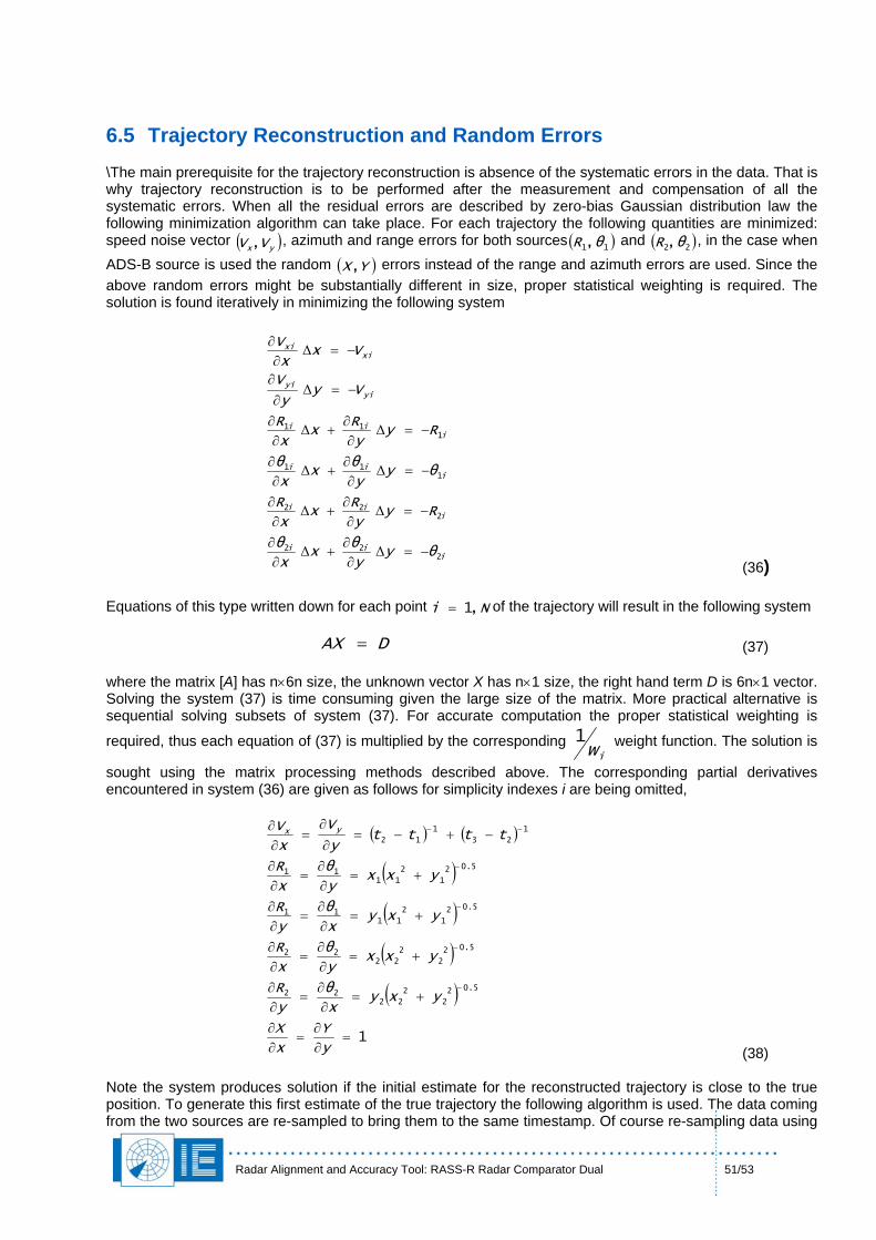
Radar Alignment and Accuracy Tool: RASS-R Radar Comparator Dual 51/53
6.5 Trajectory Reconstruction and Random Errors \The main prerequisite for the trajectory reconstruction is absence of the systematic errors in the data. That is why trajectory reconstruction is to be performed after the measurement and compensation of all the systematic errors. When all the residual errors are described by zero-bias Gaussian distribution law the following minimization algorithm can take place. For each trajectory the following quantities are minimized: speed noise vector ( ), azimuth and range errors for both sources ( )11,θRyx VV , and ( , in the case when ADS-B source is used the random ( ) errors instead of the range and azimuth errors are used. Since the above random errors might be substantially different in size, proper statistical weighting is required. The solution is found iteratively in minimizing the following system
)22,θR
YX,
iii
iii
iii
iii
yiyi
xixi
θyy
θx
x
θ
Ryy
Rx
x
R
θyy
θx
x
θ
Ryy
Rx
x
R
Vyy
V
Vxx
V
222
222
111
111
−=∂∂
+∂∂
−=∂∂
+∂∂
−=∂∂
+∂∂
−=∂∂
+∂∂
−=∂∂
−=∂∂
ΔΔ
ΔΔ
ΔΔ
ΔΔ
Δ
Δ
(36) Equations of this type written down for each point of the trajectory will result in the following system Ni ,1=
DAX = (37) where the matrix [A] has n×6n size, the unknown vector X has n×1 size, the right hand term D is 6n×1 vector. Solving the system (37) is time consuming given the large size of the matrix. More practical alternative is sequential solving subsets of system (37). For accurate computation the proper statistical weighting is
required, thus each equation of (37) is multiplied by the corresponding iw
1 weight function. The solution is
sought using the matrix processing methods described above. The corresponding partial derivatives encountered in system (36) are given as follows for simplicity indexes i are being omitted,
( ) ( )
( )
( )
( )
( )
1
5.02
2
2
2222
5.02
2
2
2222
5.02
1
2
1111
5.02
1
2
1111
1
23
1
12
=∂∂
=∂∂
+=∂∂
=∂∂
+=∂∂
=∂∂
+=∂∂
=∂∂
+=∂∂
=∂∂
−+−=∂∂
=∂∂
−
−
−
−
−−
y
Y
x
X
yxyx
θ
y
R
yxxy
θ
x
R
yxyx
θ
y
R
yxxy
θ
x
R
tttty
V
x
V yx
(38) Note the system produces solution if the initial estimate for the reconstructed trajectory is close to the true position. To generate this first estimate of the true trajectory the following algorithm is used. The data coming from the two sources are re-sampled to bring them to the same timestamp. Of course re-sampling data using
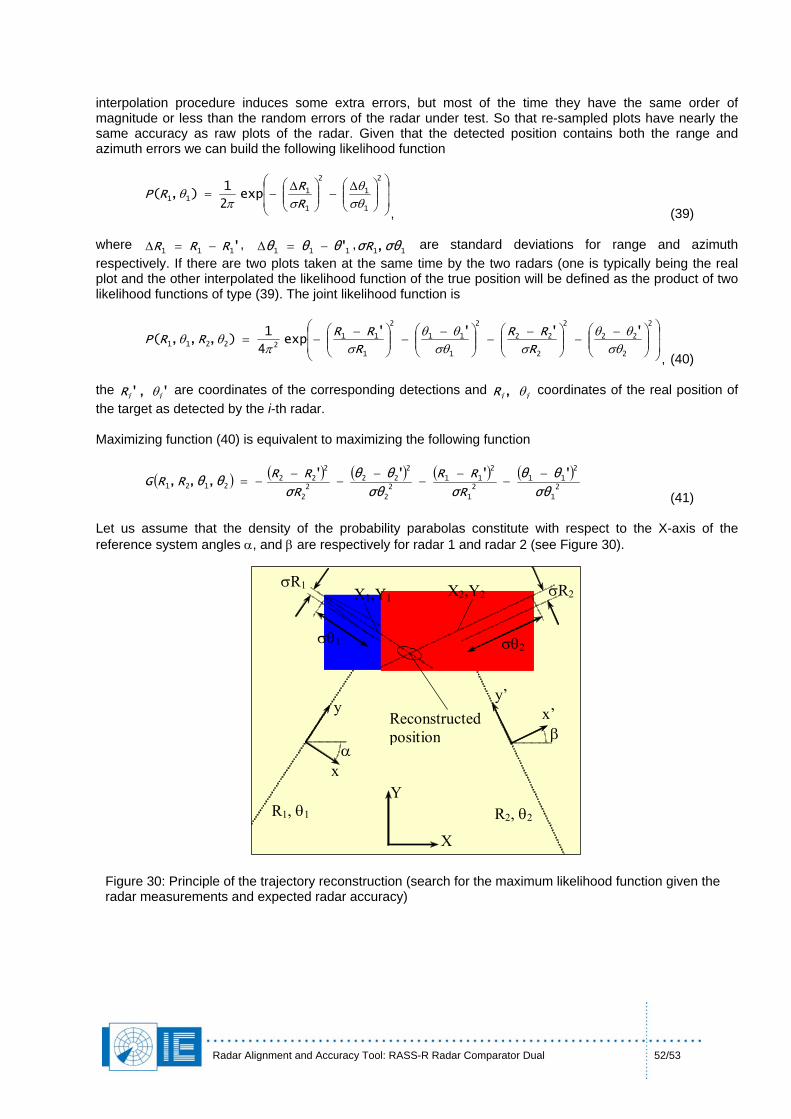
Radar Alignment and Accuracy Tool: RASS-R Radar Comparator Dual 52/53
interpolation procedure induces some extra errors, but most of the time they have the same order of magnitude or less than the random errors of the radar under test. So that re-sampled plots have nearly the same accuracy as raw plots of the radar. Given that the detected position contains both the range and azimuth errors we can build the following likelihood function
⎟⎟
⎠
⎞
⎜⎜
⎝
⎛⎟⎟⎠
⎞⎜⎜⎝
⎛ Δ−⎟⎟
⎠
⎞⎜⎜⎝
⎛ Δ−=
2
1
1
2
1
111 exp
2
1),(
σθθ
σπθ
R
RRP
, (39) where , , are standard deviations for range and azimuth respectively. If there are two plots taken at the same time by the two radars (one is typically being the real plot and the other interpolated the likelihood function of the true position will be defined as the product of two likelihood functions of type (39). The joint likelihood function is
111 'θθθ −=Δ'111 RRR −=Δ 11,σθRσ
⎟⎟
⎠
⎞
⎜⎜
⎝
⎛⎟⎟⎠
⎞⎜⎜⎝
⎛ −−⎟⎟
⎠
⎞⎜⎜⎝
⎛ −−⎟⎟
⎠
⎞⎜⎜⎝
⎛ −−⎟⎟
⎠
⎞⎜⎜⎝
⎛ −−=
2
2
22
2
2
22
2
1
11
2
1
1122211
''''exp
4
1),,,(
σθθθ
σσθθθ
σπθθ
R
RR
R
RRRRP
, (40)
are coordinates of the corresponding detections and the iiR θ,',' iiR θ coordinates of the real position of
the target as detected by the i-th radar. Maximizing function (40) is equivalent to maximizing the following function
( ) ( ) ( ) ( ) ( )2
1
2
112
1
2
112
2
2
222
2
2
222121
'''',,,
σθ
θθ
Rσ
RR
σθ
θθ
Rσ
RRθθRRG
−−
−−
−−
−−=
(41) Let us assume that the density of the probability parabolas constitute with respect to the X-axis of the reference system angles α, and β are respectively for radar 1 and radar 2 (see Figure 30).
R2, θ2R1, θ1
σR2
σθ2 σθ1
σR1
Reconstructed position
X
Y
α β
X1,Y1 X2,Y2
y y’
x
x’
Figure 30: Principle of the trajectory reconstruction (search for the maximum likelihood function given the radar measurements and expected radar accuracy)

Radar Alignment and Accuracy Tool: RASS-R Radar Comparator Dual 53/53
7. References [1] Aeronautical Telecommunications. Surveillance Radar and Collision Avoidance System, ICAO, Annex 10, Volume IV, 3rd Edition, July 2002 [2] Manual on Testing of Radio Navigation Aids, ICAO Document 8071, Volume 3, 1997 [3] EUROCONTROL Standard Document for Radar Surveillance in En-Route Airspace and Major Terminal Areas, SUR.ET1.ST01.1000-STD-01-01, 1997 [4] EUROCONTROL European Mode S Station Functional Specification, SUR/MODES/EMS/SPE-01, 2005


![Grafton Bridge Construction Traffic and Access Management ... · Construction Traffic and Access Management Plan [2] ... RASS Radar Activated Speed ... This Plan operates as the master](https://img.pdfslide.us/doc/110x75/5b4022867f8b9a5e2c8cfe39/grafton-bridge-construction-traffic-and-access-management-construction-traffic.jpg)