R7449 Final technical report Appendices - gov.uk · R7449 Final technical report Appendices ... restriction endonuclease analysis; REN ... Electrophoresis of the DNA digests were

35

R7449 Final technical report Appendices Appendices 1-2 & 4-11 are attached as electronic copies, 3 is submitted as hard copy Appendix 1 Parnell, M., Oduor, G., Ong’aro, J., Grzywacz, D., Jones, K, A. and Brown, M., (2002). The strain variation and virulence of granulovirus of diamondback moth (Plutella xylostella) isolated in Kenya. Journal of Invertebrate Pathology (in Press) Appendix 2 Grzywacz, D., Parnell, D, Kibata, G., Oduor G., Ogutu. W. O., Miano D., and Winstanley. (2002) The development of endemic baculoviruses of Plutella xylostella (diamondback moth, DBM) for control of DBM in East Africa. In “The Management of Diamond Back Moth and other Cruciferous Pests Proceedings forth International Workshop on Diamond Back Moth”, Melbourne University, Ridland, P., (Ed) (In Press) Appendix 3*Oruko, L.O., Asaba, J., F & Kindness, H. M., (2000). Factors effecting uptake and adoption of outputs of crop protection research in peri-urban vegetable systems in Kenya. In “Sustaining Change: proceedings of a workshop on the factors effecting uptake and adoption of Department for International Development Crop Protection Programme research projects” Hainsworth, S. D., and Eden-Green, S. J., (Eds.) Natural Resources International Ltd. Chatham. pp. 27-34. Appendix 4 Downham, M. C. A., (2001) An appraisal of the pheromone mating-disruption technique for management of diamond-back moth, Plutella xylostella. NRI Report. pp 41. Appendix 5*Downham, M. C. A., (2002) A second appraisal of the pheromone mating-disruption technique for management of diamond-back moth, Plutella xylostella. NRI Report. pp 31 Appendix 6* Parnell, M., (2001) Field trials of Plutella xylostella granulovirus against diamondback moth on kale, carried out in Kenya during 1998 and 2000. NRI Report pp 17. Appendix 7 Oruko, L.O., and Ndun’gu, B., (2000) Final Socio-economic report for the vegetable IPM thematic cluster. CAB International Africa Regional Centre and Kenya Agricultural Research Institute Report pp 49. Appendix 8*Ogutu, W. O., Ogol., C.K.P.O., Oduor G. I., Parnell, M., Miano, D.W. and. Grzywacz D. (2002) Evaluation of a naturally occurring baculovirus for the management of diamondback moth, Plutella xylostella L. in Kenya. Paper accepted for International symposium improving biocontrol of Plutella xylostella. 21-24th October 2002, Montpellier, France. pp 8. Appendix 9 *Grzywacz, D., Parnell, D, Kibata, G., Oduor G., Ogutu. W. O., Poole , J., and ,Miano D. (2002) The granulovirus of Plutella xylostella (diamond back moth DBM) and its potential for control of DBM in Kenya. Paper accepted for International symposium improving biocontrol of Plutella xylostella. 21-24th October 2002, Montpellier, France, pp6. Appendix 10 Kenyan application form to register a biopesticide Appendix 11 Data requirements for biopesticide registration dossier

36

The strain variation and virulence of granulovirus of diamondback moth (Plutella

xylostella, Lep., Yponomeutidae) isolated in Kenya.

Mark Parnell1, G. Oduor

2, J. Ong'aro

3, D. Grzywacz

1, K. A. Jones

1 and M. Brown

1

1: Natural Resources Institute, Central Avenue, Chatham Maritime, Kent ME4 4TB,

UK.

2: CAB International, Africa Regional Centre, PO Box 633, Village Market, Nairobi

Kenya.

3: Kenya Agricultural Research Institute, Waiyaki Way, PO Box 14733, Nairobi, Kenya.

Mr Mark Parnell

Tel: 01634 883255

Fax: 01634 883379

E-mail: [email protected]

Running title: Granulovirus of diamondback moth

Key words: Diamondback moth; Plutella xylostella; granulovirus; GV; PxGV; bioassay;

restriction endonuclease analysis; REN; EcoR1; Pst1; Kenya; Taiwan.

SUMMARY

The diamondback moth (DBM), Plutella xylostella, is a serious pest of brassica crops

throughout the world. In Kenya, control of DBM on brassica vegetables is becoming an

increasing problem due to escalating resistance to the favoured control option, chemical

37

insecticides. Plutella xylostella granulovirus (PxGV) has shown promise for DBM

control in other countries and is important as an alternative control method for future

development, however the Kenyan authorities do not allow importation of exotic

organisms for pest control purposes. Therefore, in order to test the potential of PxGV in

Kenya, isolates of this virus indigenous in Kenya had to be found. During a survey of 27

farms in Kenya, 127 diseased or dead DBM larvae were collected from several different

locations on the outskirts of Nairobi. Of the 127 samples, 95 were found to be infected

with PxGV. Restriction Endonuclease analysis of the viral DNA from infected larvae

showed that fourteen of the 95 isolates had between 2 and 6 major band differences in

DNA profiles after digestion with EcoR1 and Pst1 restriction enzymes and varied in

molecular weight by up to 6.2 kilobase pairs. Bioassays to compare the efficacy of the

Kenyan PxGV strains to each other and to a PxGV strain isolated in Taiwan found that no

significant difference in potency existed between any of the isolates. This study forms

the basis for future evaluation of PxGV‟s potential as a control agent of DBM in Kenya,

and the genetic variation in Kenyan PxGV isolates provides additional support to the

theory that DBM may have originated in southern Africa.

38

INTRODUCTION

The diamondback moth (DBM) Plutella xylostella, feed only on plants from the family

Brassicaceae and are a major pest of brassica vegetables (kale, cabbage, rapeseed etc.)

throughout Kenya (Michalik, 1994). Presently, conventional chemical insecticides are

heavily relied upon to control them (Kibata, 1997). It is well known that DBM has

become resistant to chemical insecticides in many countries throughout the world (Roush,

1997) and current programmes underway in Kenya have indicated that chemical

resistance in DBM is also occurring there (Kibata, 1997). The chemical insecticides

currently recommended for control are expensive, damaging to the environment and in

some areas simply not available to the small-scale farmers who account for a high

percentage of the brassica vegetable production of Kenya (pers. comm., Kibata). For

these reasons a collaborative project between the Natural Resources Institute (NRI), the

Kenya Agricultural Research Institute (KARI) and CAB International, Africa Regional

Centre (CABI-ARC) was set up to investigate alternative methods of DBM control. One

component of the project concentrated on the possibility of using baculoviruses.

In the past, baculoviruses (BV) have been found to infect DBM populations in India

(Rabindra, 1997), South East Asia (Kadir et. al 1999a) and the Far East (Asayama and

Osaki, 1970; Yen and Kao 1972;). Although nuclearpolyhedrovirus (NPV) of Galleria

mellonella and Autographa californica have shown pathogenicity to DBM (Kadir, 1992)

the only DBM specific BVs found have been granuloviruses (GV), most of which have

been isolated from DBM populations in South East Asia and the Far East (Asayama and

Osaki, 1970; Yen and Kao 1972; Kadir et. al 1999a). Rules laid down by the Kenyan

authorities on the importation and use of insect pathogens in Kenya stipulate that only

39

indigenous material may be used for any pest control or experimental purposes.

Therefore, under Project ZA0078 funded by the Department for International

Development (DFID) Crop Protection Program a screening programme for local isolates

of BV in Kenyan DBM populations was undertaken. The program concentrated on

screening for GV although the possibility of NPV infection was not ignored.

MATERIALS AND METHODS

Individual DBM larvae showing symptoms of GV infection were collected from field

DBM populations and after confirmation of GV presence by microscopy, restriction

endonuclease analysis (REN) of the viral DNA was performed. Laboratory bioassays of

isolates with different DNA profiles were also performed. From here on, GV samples

extracted from infected individuals will be referred to as isolates. In order to compare the

Kenyan isolates of Plutella xylostella GV (PxGV) to a standard, we used an isolate of

Taiwanese PxGV (PxGV-Tw) kindly supplied in 1992 by Horticultural Research

International (HRI) UK and previously reported on by Kadir (Kadir et. al, 1999a and b).

Prevalence of baculovirus in field collected DBM larvae

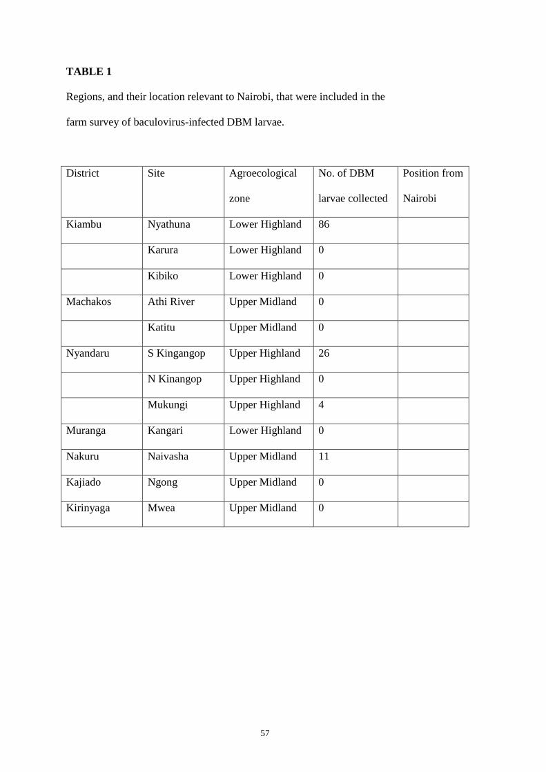
To collect GV infected DBM larvae, a survey of brassica farms was conducted which

concentrated on the region around Nairobi. In total, 27 farms were surveyed in different

agroecological (AEZ) zones in seven districts at sites within a radius of 170 km from

Nairobi (Table 1). The AEZs visited were Upper Highland (UH), Lower Highland (LH)

and Upper Midland (UM) as characterised by agroclimatic factors and soil types (Jaetzold

and Schmidt, 1983). The area to the north of the city was surveyed most intensively

40

because the cooler, wetter climate created good conditions for farmers to grow brassica

crops. DBM larvae infected with GV show very distinct symptoms, exhibiting puffy,

elongated integument and a change of colour from dull green to pale yellow (Asayama

and Osaki, 1970). Such symptoms allowed easy detection of GV infected larvae and each

larva suspected of being infected was collected individually in a 1.5ml plastic, capped

tube with no additives. All samples were kept refrigerated away from direct light until

microscopic examination was possible. Standard, unstained wet mounts of GV infected

larvae crushed in 0.5ml of sterile distilled water were examined in the laboratory using a

microscope and dark-field contrast at X400 magnification to detect the presence of GV or

NPV. All larval samples that were confirmed as having GV infection were selected for

further study and given a GV isolate number.

Propagation of GV isolates

To provide enough material for REN analysis and bioassays, each of the virus isolates

had to be multiplied. Multiplication of the virus was done in laboratory reared DBM

larvae from a colony originating from Kenya. For each isolate 15 second instar DBM

larvae were inoculated with GV by painting the virus suspension onto both surfaces of a

10.0cm x 5.0cm Chinese Cabbage leaf at a concentration of 4.0x107 GV occlusion bodies

(OB)/ml. To allow even coverage of the waxy leaf surfaces virus suspensions of GV

were in 0.01% (v/v) Triton X100 wetting agent in distilled water. Larvae were allowed to

feed on the dosed leaves for 24 hours before being transferred to fresh undosed leaves.

They were then reared until full GV infection had taken place and were harvested just

prior to death. To ensure the virus was propagated unchanged, DNA profiles of progeny

41

and inoculum viral DNA of several isolates were obtained and checked for differences in

banding patterns, none were observed.

Extraction and purification of GV from infected DBM

Larvae infected with individual GV isolates were pooled but each isolate was treated

separately to ensure no cross contamination occurred. The progeny virus from each

isolate was then extracted and purified by macerating larvae with a small mortar and

pestle, filtering the resulting suspension and centrifuging the filtrate on 50 to 70 %

sucrose following methods described by Parnell (1999b).

Restriction endonuclease analysis (REN) of GV isolates

REN analysis was performed on each of the GV isolates individually and broadly

followed a protocol devised by Smith and Summers (1978). DNA extraction was

performed on each virus isolate by addition of 25 l of 0.5 molar (M) EDTA (pH 8) and

3.0 l of proteinase K for 1.5 hours at 37 C, followed by 75 l of 1M sodium carbonate

(15 minutes) and 25 l of 10% (w/v) sodium dodecyl sulphate (30 minutes). After

treatment with equal volumes of tris-saturated phenol:chloroform:isoamyl alcohol

(25:24:1) and chloroform:isoamyl alcohol (24:1), the extracted DNA was purified by

dialysis in tris-acetate buffer (pH 8.3) at 4 C for 36 hours. Restriction enzyme digestions

(EcoR1 and Pst1) were performed on the purified DNA of all virus isolates as specified

by the manufacturer (Promega UK Ltd, Delta House, Southampton. S07 7NS).

Electrophoresis of the DNA digests were then carried out at 35 volts for 18 hours on 0.6%

agarose gels prepared with tris-acetate buffer (pH 8.3) and suspended in tris-acetate

42

buffer-filled electrophoresis tanks. The PxGV-Tw standard and molecular weight

markers (1 kilobase, Life Technologies, and mix 19, MBI Fermentas) were run along

side the DNA digests on each gel. DNA profiles were stained by submerging the agarose

gels in ethidium bromide solution (100 l in 1 litre distilled water) for 30 minutes. DNA

profiles of each isolate present in the gels were displayed on an ultra violet

transiluminator (Camlab Ltd., Cambridge. CB4 1TH. UK.) and photographs were taken

using a Polaroid MP-4 Land Camera with 667 black and white film. Approximate

molecular weights of genomes of the GV isolates were estimated from the mobility of

DNA fragments relative to fragments of 1Kb ladder and Mix19 molecular weight

markers (MBI Fermentas, Helena Biosciences, Sunderland, UK).

Comparative pathogenicity bioassays

Test larvae

DBM larvae were used in all bioassays. The larvae used were from a disease free

laboratory colony that had been established at NRI from wild Plutella xylostella pupae

collected from the Ngong region of Kenya in 1996. The colony was maintained on 4-6

week old Chinese Cabbage seedlings at 25 C ( 2 C) under a 12:12 light:dark cycle in

clear Perspex cages with cut-out sides covered in muslin for ventilation. To ensure larvae

used in the assays were of the same age, fresh seedlings were presented to the adults on a

daily basis so that eggs from a single day's lay could be collected. Second instar larvae

were chosen for bioassay having first scrutinised the head capsule size to be sure of

collecting the desired larval stage.

43

Bioassay Procedure

The pathogenicity of the different isolates were determined by means of two bioassay

methods. Initially comparative bioassays using single discriminate doses aimed at

producing between 20 and 70% mortality in test insects were performed on eight GV

isolates displaying different DNA profiles in order to ascertain if significant differences in

potency existed. Subsequently, in order to obtain LC50 values, dose series bioassays were

carried out on three of those eight isolates and the PxGV-Tw isolate. For the discriminate

dose bioassays a single dose of each of the nine isolates tested was prepared in 0.01%

Triton X100 at a concentration of between 2.10 x 106 OB/ml and 5.40 x 10

6 OB/ml.

Although the doses were not prepared to exactly the same concentration for every isolate,

it was considered that to cause a significant effect in mortality levels a larger difference in

dose than was present would have been required due to the low slope of dose against

mortality in bioassays. For the three isolates used in the dose series bioassay, four five-

fold dilutions of a top concentration that fell within 2.70 x107

OB/ml and 3.06 x 108

OB/ml were prepared. Doses were prepared by dilution of purified stock suspension of

each isolate tested. The concentration of each was determined by counting the virus

using a 0.02mm depth, bacterial spore counting chamber (Weber Scientific International,

UK) and a Leica DMRB microscope set to dark phase illumination at x200 magnification.

A leaf paint bioassay method was used in both procedures whereby 150 l of virus

suspension of each dose was applied to Chinese cabbage leaves of 50mm x 70mm

ensuring both surfaces were completely and uniformly covered. Once the virus had dried,

leaves were mounted in 10 mls of 0.8% (w/v) molten agar. Dosed leaves were mounted

by the stem only, in clear plastic 90mm diameter tubs. Two leaves were prepared for

each dose of the isolates tested and 15 second instar DBM larvae were placed on each leaf

44

(30 larvae/dose) before lids were placed on the tubs. The lids were ventilated with 15

slits produced by a No. 11 scalpel blade and the assays were incubated at 27 C in a 12:12

night:day cycle. After 24 hours of feeding on infected leaf material, all larvae were

transferred to freshly mounted, undosed Chinese cabbage leaves and were supplied fresh

feeding material as when it was required. The bioassays were run until death or pupation

of all larvae and daily monitoring was carried out of larval mortality to monitor speed of

kill.

RESULTS

Prevalence of baculovirus in field collected DBM larvae

During the field survey, 127 larvae with disease symptoms were collected from eight of

the 27 farms included in the survey. Microscopic examination confirmed that 95 larvae

collected from four of the eight farms were suffering from GV infection. The areas in

which GV-infected larvae were found covered all three agroecological zones visited and

were Nyathuna, South Kinangop and Naivasha. In Nyathuna, 84 GV-infected DBM

larvae were collected (isolates Nya-01 to Nya-84), in South Kinangop 9 GV infected

larvae were collected (isolates SK-01 to SK-09) and in Naivasha 2 GV-infected larvae

were collected (isolates Nva-01 and Nva-02).

Restriction endonuclease analysis of GV infected DBM

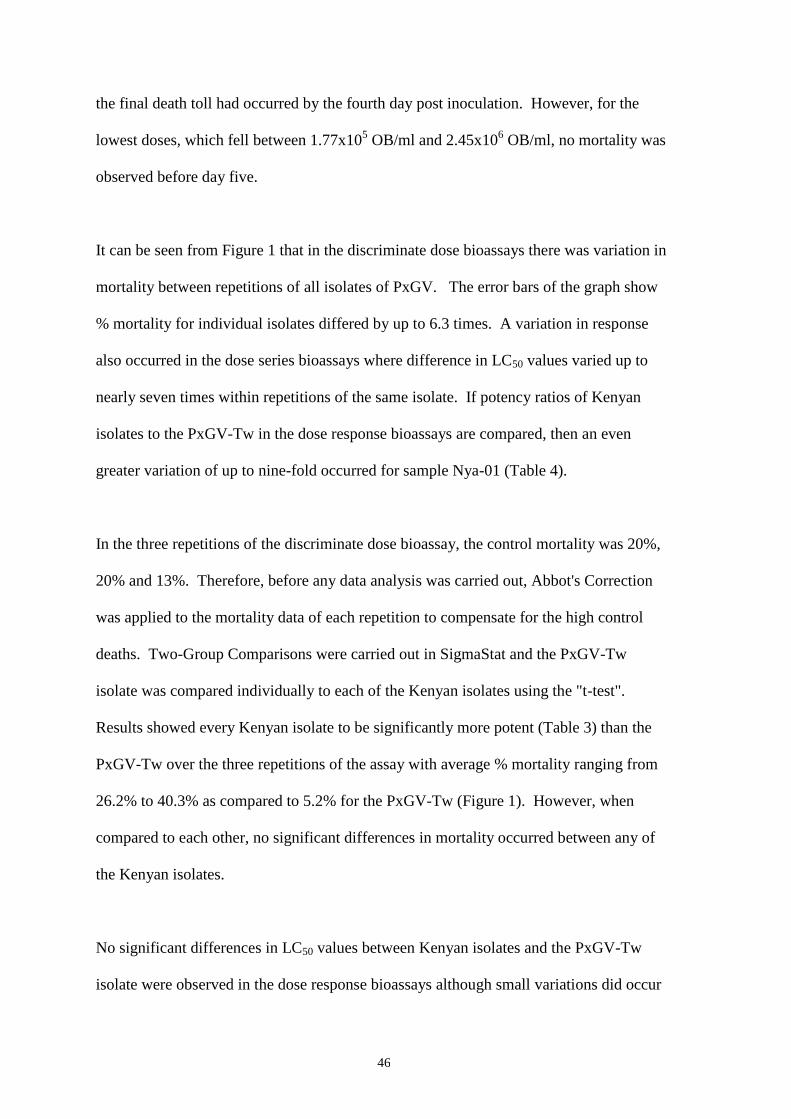
The REN analysis of the 95 PxGV isolates showed that 27 had different DNA fragment

profiles to any other when cut with either one of the two restriction enzymes. Of those

45

27, 14 had fragment profiles that could be distinguished from any other with both EcoR1

and Pst1 cuts (Figure 2). Comparison of these 14 Kenyan PxGV isolates to an isolate of

PxGV from Taiwan (PxGV-Tw) revealed that, although the profiles had many

similarities, there were major band differences between all isolates. Both the Pst1 and

EcoR1 digests revealed between 2 and 6 major band differences between isolates, even in

those collected from the same location (Figure 2).

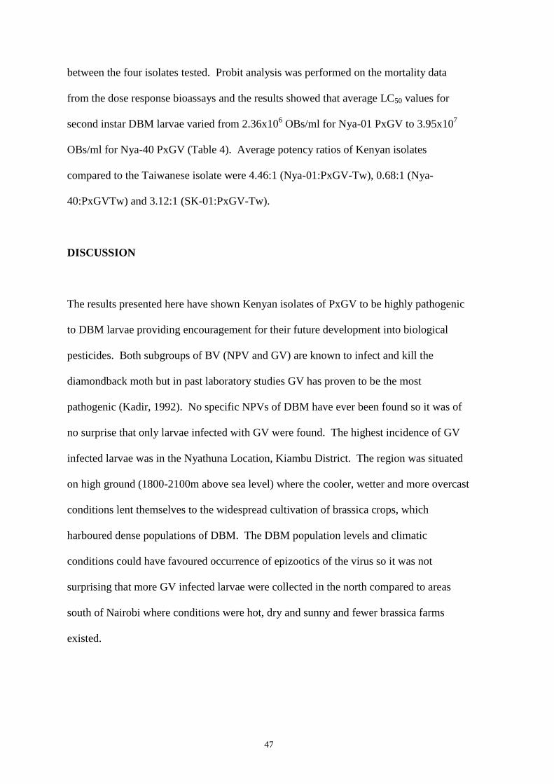
The level of variation in banding patterns between the PxGV-Tw and any Kenyan isolate

was no greater than that seen when comparing Kenyan isolates to each other. The

dendrogram in Figure 3 shows the level of homology between the Kenyan and Taiwanese

isolates and it can be seen that the PxGV-Tw isolate shares a closer homology to many of

the Nyathuna Kenyan isolates than the South Kinangop isolate (SK-01) does. Table 2

presents the estimated molecular weights of all isolates with a different DNA profile. It

can be seen that the estimated molecular weights of the Kenyan isolates varied from

92.12 kilobase pairs (kbp) (Nya-52) to 98.32 kbp (Nya-40). The Taiwanese isolate had

the lowest molecular weight at 90.71 kbp.

Pathogenicity of different PxGV isolates

Although no lethal time (LT) experiments were conducted the results of bioassays

indicated that speed of kill did not vary significantly between any of the Kenyan isolates

when compared to the Taiwanese standard or each other. The bioassays showed that time

to death ranged from 4 to 8 days post inoculation but in the dose series bioassays speed of

kill was generally fastest for high doses. The dose series bioassays showed that for the top

concentrations, which fell between 2.70 x107

OB/ml and 3.06 x 108 OB/ml, up to 100% of

46

the final death toll had occurred by the fourth day post inoculation. However, for the

lowest doses, which fell between 1.77x105 OB/ml and 2.45x10

6 OB/ml, no mortality was

observed before day five.

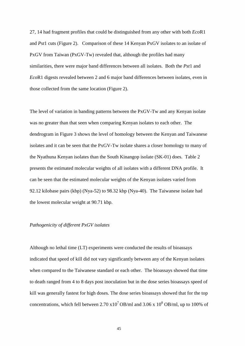
It can be seen from Figure 1 that in the discriminate dose bioassays there was variation in

mortality between repetitions of all isolates of PxGV. The error bars of the graph show

% mortality for individual isolates differed by up to 6.3 times. A variation in response

also occurred in the dose series bioassays where difference in LC50 values varied up to

nearly seven times within repetitions of the same isolate. If potency ratios of Kenyan

isolates to the PxGV-Tw in the dose response bioassays are compared, then an even

greater variation of up to nine-fold occurred for sample Nya-01 (Table 4).

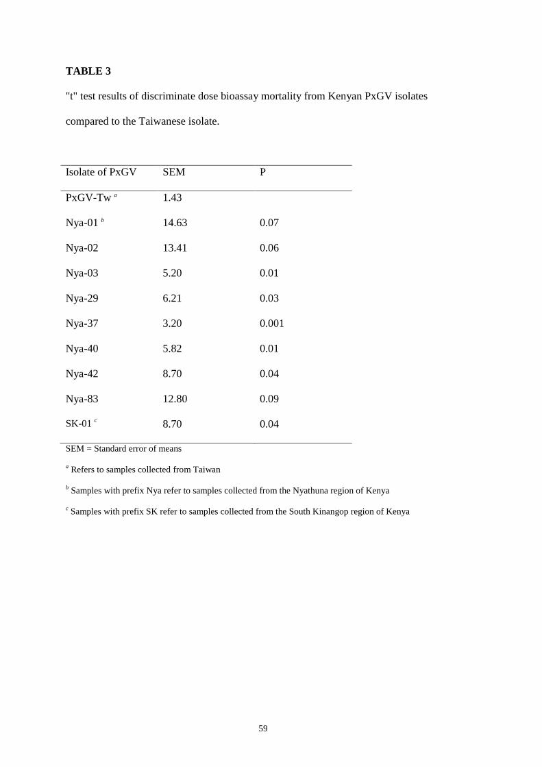
In the three repetitions of the discriminate dose bioassay, the control mortality was 20%,

20% and 13%. Therefore, before any data analysis was carried out, Abbot's Correction

was applied to the mortality data of each repetition to compensate for the high control

deaths. Two-Group Comparisons were carried out in SigmaStat and the PxGV-Tw

isolate was compared individually to each of the Kenyan isolates using the "t-test".

Results showed every Kenyan isolate to be significantly more potent (Table 3) than the

PxGV-Tw over the three repetitions of the assay with average % mortality ranging from

26.2% to 40.3% as compared to 5.2% for the PxGV-Tw (Figure 1). However, when

compared to each other, no significant differences in mortality occurred between any of

the Kenyan isolates.

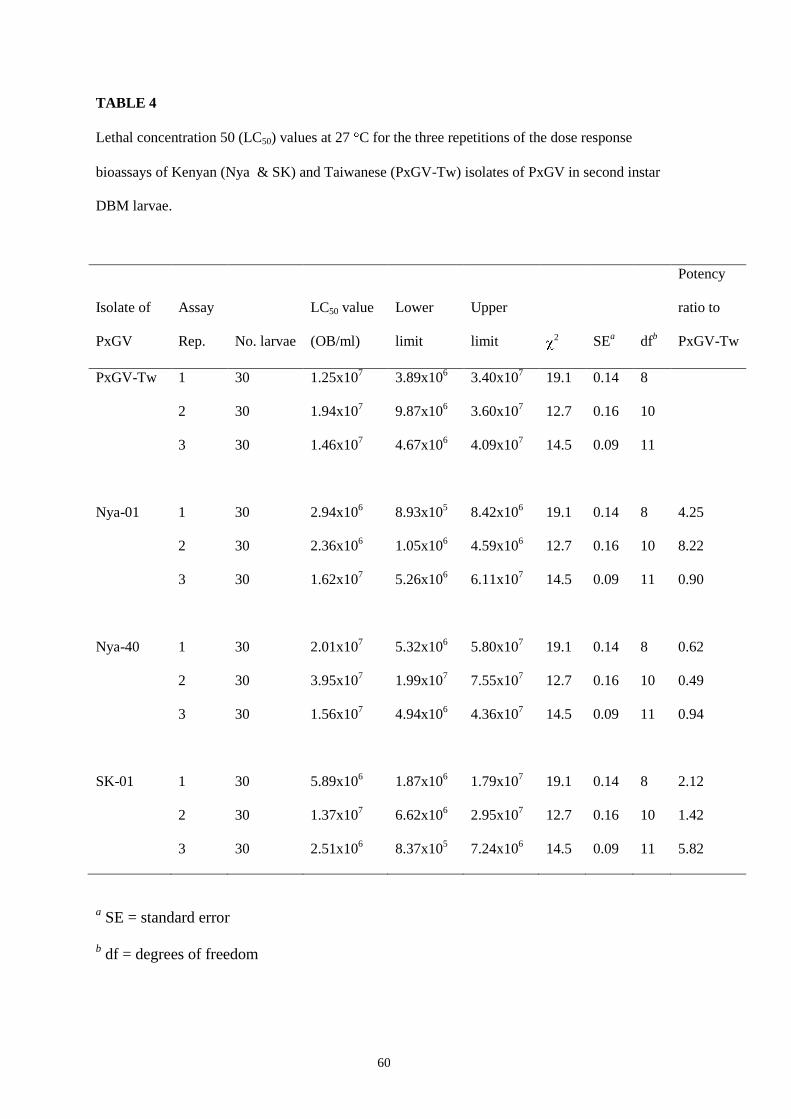
No significant differences in LC50 values between Kenyan isolates and the PxGV-Tw

isolate were observed in the dose response bioassays although small variations did occur

47

between the four isolates tested. Probit analysis was performed on the mortality data

from the dose response bioassays and the results showed that average LC50 values for

second instar DBM larvae varied from 2.36x106 OBs/ml for Nya-01 PxGV to 3.95x10

7

OBs/ml for Nya-40 PxGV (Table 4). Average potency ratios of Kenyan isolates

compared to the Taiwanese isolate were 4.46:1 (Nya-01:PxGV-Tw), 0.68:1 (Nya-

40:PxGVTw) and 3.12:1 (SK-01:PxGV-Tw).

DISCUSSION

The results presented here have shown Kenyan isolates of PxGV to be highly pathogenic

to DBM larvae providing encouragement for their future development into biological

pesticides. Both subgroups of BV (NPV and GV) are known to infect and kill the

diamondback moth but in past laboratory studies GV has proven to be the most

pathogenic (Kadir, 1992). No specific NPVs of DBM have ever been found so it was of

no surprise that only larvae infected with GV were found. The highest incidence of GV

infected larvae was in the Nyathuna Location, Kiambu District. The region was situated

on high ground (1800-2100m above sea level) where the cooler, wetter and more overcast

conditions lent themselves to the widespread cultivation of brassica crops, which

harboured dense populations of DBM. The DBM population levels and climatic

conditions could have favoured occurrence of epizootics of the virus so it was not

surprising that more GV infected larvae were collected in the north compared to areas

south of Nairobi where conditions were hot, dry and sunny and fewer brassica farms

existed.

48

Although there were sixteen different DNA profiles identified from the 95 isolates

collected on the survey and distinguished by both restriction enzymes, in most cases each

profile was present in more than one infected larva. Only one isolate (SK-01) was found

to be infecting just a single larva and from the dendrogram in Figure 3, it can be seen that

its profile was the least homologous when compared with the others. The isolate was not

significantly less potent than any others included in the dose response assays and its DNA

profile did not possess any sub-molar bands so it is unlikely to be a mixture of two

competing isolates. However, it was unusual to find an isolate infecting only one larva

when the others were all found in several.

The similarities observed between the Taiwanese and Kenyan isolates are consistent with

those observed in a previous study of the same Taiwanese isolate, in which it was

compared to a Chinese isolate of PxGV (Kadir et. al, 1999a). Kadir noted that they

appeared very closely related although he did observe between 1 and 3 major band

differences between the two isolates after digestion with EcoR1, HindIII and BamH1.

The level of variation between isolates in Kadir‟s study was less than that seen between

some isolates collected from the same sites in Kenya even though the Kadir isolates were

from two different countries. The high level of variation in the same Kenyan site could

indicate a long association between GV and DBM in the region. No such variation has

been reported previously and in a field survey carried out in Japan, only one isolate of

PxGV was discovered (Yamada and Yamaguchi, 1985). The theory that DBM is an

exotic pest in the Far East allows the hypothesis that its diseases travelled with it, and that

the PxGV found in Taiwan and China could have originated elsewhere.

49

The origin of DBM is generally considered to be somewhere in Mediterranean Europe

having evolved on cultivated brassicas also believed to have European origin (Hardy,

1938). Recently however, the origin of DBM has been brought into question by Kfir

(1998) who noted that 175 wild plant species belonging to the family Brassicaceae have

been recorded in South Africa. He also conducted a survey of wild DBM populations in

South Africa in which he isolated 22 species of parasitoids and hyperparasitoids. Some

of those were found to be specific to DBM and restricted to South Africa. In particular

the sexual form of the parasitoid Diadromus collaris, which only appears in an asexual

form in Europe. Considering that all asexual organisms derive from sexual forms (Mayr,

1965), the author speculated that the diverse fauna of DBM parasitoids and

hyperparasitoids, large number of indigenous host plants and existence of the sexual form

of Diadromus collaris provided compelling evidence that the origin of DBM was

southern Africa. The wide variation in genomes of PxGV isolates discovered in Kenya

during the present study and apparent lack of diversity in isolates from other regions of

the world provides additional support to the theory that the origin of DBM lies in Sub-

Saharan Africa.

The information gathered on speed of kill did not show any significant differences

between isolates but as other studies have shown a certain degree of dose dependency

existed (van Beek et. al, 1988; Kadir et. al, 1999b). Kadir‟s study showed a dose

dependency existed in bioassays of first instars although the assays performed on second

instars did not show a similar trend. Kadir performed 18 repetitions of assays on first

instars but only 2 on second instars and commented that dose dependency for time to

death was generally only observed where an extensive number of assays had been

performed. It is possibly the case that a large number of repetitions are required to show

50

up trends in dose dependency on time to death. However, only three replicates of the

dose response assay in the current study were performed so it may be the case that a dose

dependency on time to death does exist in PxGV assays.

The level of response varied considerably in all of the bioassays carried out with up to a

seven-fold difference on some occasions. Although no precision tests of the bioassay

method were carried out, the level of variation in response was comparable to that shown

in other studies involving bioassay of DBM pathogens in which extensive precision tests

were done and found to be within acceptable levels (Kadir et. al, 1999b). Kadir found

that mean LD50 value varied up to almost nine-fold from 1.0 to 8.9 OB per neonate larva

in a series of bioassays consisting of 18 repetitions. Therefore, the present study showed

a similar level of variation to kadir's.

Although the initial discriminate dose bioassays indicated that the Kenyan isolates were

all more potent than the Taiwanese isolate the more rigorous dose response method did

not support this. There have been no comparative studies of the pathogenicity of different

PxGV isolates to DBM larvae in the past although similar results were obtained in studies

of GV isolates of other insect species (Crook, 1986; Crook et. al 1985). In Crook's

studies, the infectivity of five isolates Artogeia rapae GV (ArGV) and three different

isolates of Cydia pomonella GV (CpGV) from different geographical locations were

investigated and showed no significant difference in potency between any of the isolates

tested. There were no significant differences in potency between any Kenyan isolate

indicating that the high level of variation between isolates had no discernible effect on

potency. Such a variability in GV could be highly beneficial in the development of future

51

PxGV-based DBM control strategies in that variation of isolate may be used in resistance

management practices.

Many countries have strict rules on importation of exotic organisms for use as pest

control measures and in some, the precise legislation is patchy or confused with a blanket

ban on exotic isolates creating difficulties in registration of existing products or testing of

novel ones. In many cases the restriction on importation of exotics is essential, however,

the authors would like to bring the following points to attention. The REN analysis

showed that although variation existed between Kenyan and the Taiwanese isolates, many

shared a high proportion of similar restriction sites. In fact, there was a greater level of

variation between some Kenyan isolates than between Kenyan and the Taiwanese isolate.

In addition to that, the bioassays showed no significant difference in activity between any

isolate be it from Kenya or Taiwan. Such results indicate that a high level of affinity

between isolates from different geographical locations may exist. In such circumstances

there would appear to be room for relaxation of certain aspects of legislation on

importation of exotic organisms, so long as those organisms were in an original and

unaltered state and could be shown to share a high affinity with indigenous isolates.

The average LC50 value of the Taiwanese isolate was 7.8 times greater in the present

study than was found in a previous study of the same isolate (Kadir et. al, 1999b). In

comparison, the LC50 values of the Kenyan isolates were between 3.6 and 12.5 times

greater than Kadir‟s figures. In his study, Kadir noted that the LC50 value of the

Taiwanese strain of PxGV placed it amongst GV isolates that are highly infectious to

their hosts (Payne, 1986; Payne et. al, 1981). Therefore, considering the lack of

significant difference found between Kenyan and Taiwanese isolates, the Kenyan isolates

52

should also be considered in the same group. It is generally considered that highly

infectious GV isolates are suitable for use as control products of their hosts, thus justify

the further development of Kenyan PxGV as a DBM control measure.

ACKNOWLEDGEMENTS

We would like to thank the many staff of KARI and CABI-ARC for their assistance and

support in conducting surveys and field trials in Kenya. This publication is an output from

a research project originally prepared by Dr Andy Cherry of NRI, which was funded by

the Department for International Development of the United Kingdom (DFID). However,

the Department for International Development can accept no responsibility for any

information provided or views expressed. DFID project R 6615 - Crop Protection

Program.

REFERENCES

Asayama, T. and Osaki, N. 1970. A granulosis of the diamondback moth, Plutella

xylostella. J. Invertbr. Pathol. 15, 284-286.

Crook, N.E. 1986. Restriction enzyme analysis of granulosis viruses isolated from

Artogeia rapae and Pieris brassicae. J.Gen. Virol. 67, 781-787.

53

Crook, N.E., Spencer, R.A., Payne, C.C., and Leisy, D.J. 1985. Variation in Cydia

pomonella granulosis virus isolates and physical maps of the DNA from three variants.

J. Gen. Virol. 66, 2423-2430.

Hardy, J.E. 1938. Plutella maculipennis Curt. Its natural and biological control in

England. Bull. of Entomol. Res. 29, 343-372.

Jaetzold, R. and Schmidt, H. 1983. Farm management handbook, volII, natural

conditions and farm management information, Part B. Minsitry of Agriculture, Kenya.

Kadir, H.A. 1992. Potential of several baculoviruses for the control of diamondback moth

and Crocidolomia binotalis on cabbages. In Talekar, N.S. (Ed), Diamondback Moth

and Other Crucifer Pests. Proceedings of the Second International Workshop, Tainan,

Taiwan, 10-14 December 1990. AVRDC Publications, Taipei, pp 185-192.

Kadir, H.A., Payne, C.C., Crook, N.E., and Winstanley, D. 1999(a). Characterization and

cross-transmission of baculoviruses infective to the diamondback moth, Plutella

xylostella, and some other Lepidopterous pests of brassica crops. Biocontrol Sci.

Technol. 9, 227-238.

Kadir, H.A., Payne, C.C., Crook, N.E., Fenlon, J.S., and Winstanley, D., 1999(b). The

comparative susceptibility of the diamondback moth, Plutella xylostella, and some

other major lepidopteran pests of brassica crops, to a range of baculoviruses.

Biocontrol Sci. Technol. 9, 421-433.

54

Kfir, R. 1998. Origin of the diamondback moth (Lepidoptera: Plutellidae). Annals of the

Entomological Society of America, 91, (2), 164-167.

Kibata, G.N. 1997. The diamondback moth: A problem pest of brassica crops in Kenya.

In Sivapragasam, A, Loke, W.H., Kadir, A.H., Lim, G.S., (Eds) The Management of

Diamondback Moth and Other Crucifer Pests. Proceedings of the Third International

Workshop, Kuala Lumpur, Malaysia 29 October - 1 November, 1996. MARDI,

Malaysia, pp 47-53.

Mayr, E. 1965. Animal species and evolution. Belknap, Harvard University Press,

Cambridge.

Michalik, S. 1994. Report on crop protection measures of Kenyan vegetable farmers and

their use of pesticides: a knowledge, attitude and practical survey. KARI/GTZ IPM

Horticulture Project, p 7. Published by GTZ.

Parnell, M. A. 1999a. The genetic variability and efficacy of baculoviruses for control of

diamondback moth on brassica vegetables in Kenya. MSc Thesis, University of

Greenwich, Greenwich, UK. pp 8-21.

Parnell, M. A., 1999b. The genetic variability and efficacy of baculoviruses for control of

diamondback moth on brassica vegetables in Kenya. MSc Thesis, University of

Greenwich, Greenwich, UK. pp 72, 49-50.

55

Payne, C.C. 1986. Insect pathogenic viruses as pest control agents. Fortschritte der

Zoologie 32, 183-200.

Payne, C.C., Tatchell, G.M., and Williams, C.F. 1981. The comparative susceptibilities of

Pieris brassicae and P. rapae to a granulosis virus of virus from P. brassicae. J.

Invertebr. Pathol. 38, 273-280.

Rabindra, R.J., Geetha, N., Renuka, S., Varadharajan, S., and Regupathy, A. 1997.

Occurrence of a granulosis virus from two populations of Plutella xylostella (L.) in

India. In Sivapragasam, A, Loke, W.H., Kadir, A.H., Lim, G.S., (Eds) The

Management of Diamondback Moth and Other Crucifer Pests. Proceedings of the

Third International Workshop, Kuala Lumpur, Malaysia 29 October - 1 November,

1996. MARDI, Malaysia, pp 113-115.

Roush, T. 1997. Insecticide resistance management in diamondback moth: quo vadis? In

Sivapragasam, A, Loke, W.H., Kadir, A.H., Lim, G.S., (Eds) The Management of


Workshop, Kuala Lumpur, Malaysia 29 October - 1 November, 1996. MARDI,

Malaysia, pp 21-24.

Smith, G.E. and Summers, M.D. 1978. Analysis of baculovirus genomes with restriction

endonucleases. Virology 89, 517-527.

56

Van Beek, N.A.M., Wood, H.A., and Hughes, P.R. 1988. Quantitative aspects of nuclear

polyhedrosis virus infections in lepidopterous larvae: the dose-survival time

relationship. J. Invertebr. Pathol. 51, 58-63.

Yen, D.F. and Kao, A.H. 1972. Studies on the granulosis of the diamondback moth

(Plutella xylostella L.) in Taiwan. Mem. Coll. Agric. Natl. Taiwan Univ. 13, 172-181

(in Chinese with English summary).

Yamada, H. and Yamaguchi, T. 1985. Notes on parasites and predators attacking the

diamondback moth, Plutella xylostella. Japanese J. Appl. Entomol. and Zool. 29 (2),

170-173. (In Japanese with English summary).

57

TABLE 1

Regions, and their location relevant to Nairobi, that were included in the

farm survey of baculovirus-infected DBM larvae.

District Site Agroecological

zone

No. of DBM

larvae collected

Position from

Nairobi

Kiambu Nyathuna Lower Highland 86

Karura Lower Highland 0

Kibiko Lower Highland 0

Machakos Athi River Upper Midland 0

Katitu Upper Midland 0

Nyandaru S Kingangop Upper Highland 26

N Kinangop Upper Highland 0

Mukungi Upper Highland 4

Muranga Kangari Lower Highland 0

Nakuru Naivasha Upper Midland 11

Kajiado Ngong Upper Midland 0

Kirinyaga Mwea Upper Midland 0

58

TABLE 2

Estimated molecular weight, in kilobase

pairs, of Kenyan and Taiwanese PxGV DNA.

Sample Molecular weight

(Kb pairs)

Nya-01 PxGVc

96.679

Nya-02 PxGV 96.420

Nya-03 PxGV 95.720

Nya-06 PxGV 95.420

Nya-07 PxGV 96.720

Nya-14 PxGV 97.950

Nya-15 PxGV 97.770

Nya-25 PxGV 96.970

Nya-27 PxGV 96.120

Nya-29 PxGV 92.720

Nya-40 PxGV 98.320

Nya-42 PxGV 92.450

Nya-52 PxGV 92.120

SK-01 PxGVb 95.570

PxGV-Twa 90.710

a Refers to samples collected from Taiwan

b Samples with prefix SK refer to samples collected from the South Kinangop region of Kenya

c Samples with prefix Nya refer to samples collected from the Nyathuna region of Kenya

59

TABLE 3

"t" test results of discriminate dose bioassay mortality from Kenyan PxGV isolates

compared to the Taiwanese isolate.

Isolate of PxGV SEM P

PxGV-Tw a 1.43

Nya-01 b 14.63 0.07

Nya-02 13.41 0.06

Nya-03 5.20 0.01

Nya-29 6.21 0.03

Nya-37 3.20 0.001

Nya-40 5.82 0.01

Nya-42 8.70 0.04

Nya-83 12.80 0.09

SK-01 c 8.70 0.04

SEM = Standard error of means

a Refers to samples collected from Taiwan

b Samples with prefix Nya refer to samples collected from the Nyathuna region of Kenya

c Samples with prefix SK refer to samples collected from the South Kinangop region of Kenya

60

TABLE 4

Lethal concentration 50 (LC50) values at 27 C for the three repetitions of the dose response

bioassays of Kenyan (Nya & SK) and Taiwanese (PxGV-Tw) isolates of PxGV in second instar

DBM larvae.

Isolate of

PxGV

Assay

Rep.

No. larvae

LC50 value

(OB/ml)

Lower

limit

Upper

limit

2

SEa

dfb

Potency

ratio to

PxGV-Tw

PxGV-Tw 1 30 1.25x107 3.89x10

6 3.40x10

7 19.1 0.14 8

2 30 1.94x107 9.87x10

6 3.60x10

7 12.7 0.16 10

3 30 1.46x107 4.67x10

6 4.09x10

7 14.5 0.09 11

Nya-01 1 30 2.94x106 8.93x10

5 8.42x10

6 19.1 0.14 8 4.25

2 30 2.36x106 1.05x10

6 4.59x10

6 12.7 0.16 10 8.22

3 30 1.62x107 5.26x10

6 6.11x10

7 14.5 0.09 11 0.90

Nya-40 1 30 2.01x107 5.32x10

6 5.80x10

7 19.1 0.14 8 0.62

2 30 3.95x107 1.99x10

7 7.55x10

7 12.7 0.16 10 0.49

3 30 1.56x107 4.94x10

6 4.36x10

7 14.5 0.09 11 0.94

SK-01 1 30 5.89x106 1.87x10

6 1.79x10

7 19.1 0.14 8 2.12

2 30 1.37x107 6.62x10

6 2.95x10

7 12.7 0.16 10 1.42

3 30 2.51x106 8.37x10

5 7.24x10

6 14.5 0.09 11 5.82

a SE = standard error

b df = degrees of freedom

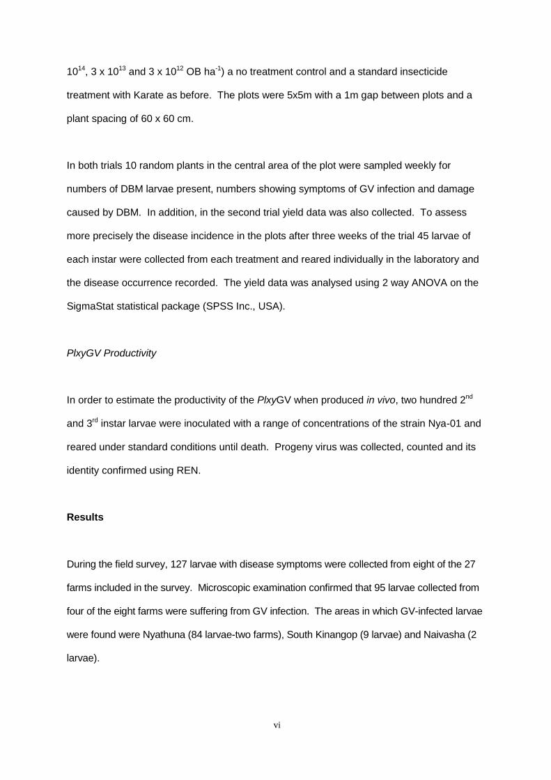
FIG. 1. Bar chart of average mortality of second instar DBM larvae expressed in

discriminate dose bioassays of Kenyan and Taiwanese PxGV. Error bars are standard

deviations.

FIG.2. Comparison of PxGV isolates. DNA of each isolate was digested with Pst1

restriction endonuclease, fragments were separated on 0.6% agarose gel. Track 1, 1kb

molecular size standard; tracks 2-16, Kenyan PxGV isolates from Nyathuna (Nya-01, Nya-

02, Nya-03, Nya-06, Nya-07, Nya-14, Nya-15, Nya-25, Nya-27, Ny-29, Nya-35, Nya-37,

Nya-40, Nya-42, Nya-52 respectively); track 17, PxGV isolate from South Kinangop (SK-

01); track 18, Taiwanese PxGV; Track 19, 19-Mix molecular size standard.

Note: Track 12 (Nya-35) is a mixed isolate with profiles of Nya-29 and Nya-42 (Tracks 11 and 15). Track 13

(Nya-37) has the same profile as Nya-52 (Track 16).

FIG. 3. Dendrogram showing homology between Kenyan and Taiwanese PxGV isolates.

“Tw” is the Taiwanese PxGV-Tw isolate, “Nya” prefix represents samples collected in the

Nyathuna region of Kenya, “SK” prefix represents samples collected from the South

Kinangop region of Kenya.

ii

The development of endemic baculoviruses of Plutella xylostella (diamond back moth

DBM) for control of DBM in East Africa.

David Grzywacz1, Mark Parnell 1, Gilbert Kibata2, George Odour3, Walter Ogutu3,Douglas

Miano2.& Doreen Winstanley4.

1: Sustainable Agriculture Group, Natural Resources Institute, University of Greenwich,Central

Avenue, Chatham Maritime, Kent ME4 4TB, UK.


3: CAB International, Africa Regional Centre, PO Box 633, Village Market, Nairobi Kenya.

4: Horticultural Research International, Wellesbourne, Warwickshire,

CV35 9EF UK.

Abstract

A project to develop non-chemical methods of DBM control on brassica crops in Kenya has

been exploring the use of endemic pathogens as potential control agents. Initial surveys for

endemic pathogens identified P.xylostella granulovirus (PlxyGV) on farms in Kenya.

Subsequently 14 genetically distinguishable isolates were identified from field collected

material. These were purified and ranging bioassays showed these isolates were

pathogenic to Kenyan strains of DBM with LC50’s varying from 2.36x106 to 3.95x107 occlusion

bodies (OB) per ml for second instar DBM. One isolate (Nya-01) was selected and

subsequently used for field trials in Kenya. The trials showed that unformulated PlxyGV

applied at weekly intervals at a rate of 3.0 x1013 OB/ha could control DBM on Kale more

effectively than available chemical insecticides. After application, infection rates in DBM can

reach 90%. Further field trials are currently underway to determine the lowest effective dose

rate for this virus when applied as a formulation. Initial virus production studies using in vivo

iii

propagation in 2nd instar DBM reared on cabbage showed an initial productivity of 4.0 0.44

x1010 OB per larva.

Keywords Plutella xylostella, baculovirus, brassicae, granulovirus, biocontrol, Kenya,

Running title Development of endemic baculoviruses of DBM in Kenya

Introduction

The diamondback moth (DBM) Plutella xylostella, feed only on plants from the family

Brassicaceae and are a major pest of brassica vegetables (kale, cabbage, rapeseed etc.)

throughout Kenya (Michalik, 1994). Presently, conventional chemical insecticides are

heavily relied upon to control them (Kibata, 1997). It is well known that DBM has become

resistant to chemical insecticides in many countries throughout the world (Roush, 1997) and

current programmes underway in Kenya have indicated that chemical resistance in DBM is

also occurring there (Kibata, 1997). The chemical insecticides currently recommended for

control are expensive, damaging to the environment and in some areas simply not available

to the small-scale farmers who account for a high percentage of the brassica vegetable

production of Kenya (Kibata 1996).

To address this issue, a collaborative project between the Natural Resources Institute (NRI),

the Kenya Agricultural Research Institute (KARI) and CAB International, Africa Regional Centre

(CABI-ARC) was set up to investigate alternative methods of DBM control. One component of

the project investigated the possible use of endemic baculoviruses.

Before this study GVs of P.xylostella had been reported from Japan (Asayama and Osaki

1970) Taiwan (Wang & Rose 1978, Kadir 1986), China (Kadir et al 1999) and India

(Rabindra 1997) but there were no previous published records from Africa. A number of

iv

other NPVs, some uncharacterised (Padamvathamma and Veeresh 1989), have been

reported as infecting DBM but a review of the potential of DBM pathogens concluded that

only the GV showed promising levels of pathogenicity (Wilding 1986). More recently an NPV

has been identified from P.xylostella in China. This was characterised as being genetically

similar to, though genetically distinct from, Autographa californica MNPV and A.falcifera

MNPV (Kariuki and McIntosh 1999).

Materials and methods

Pathogen survey and identification

To collect baculoviruses a survey of brassica farms was conducted around Nairobi. In total,

27 farms were surveyed within a radius of 170 km from Nairobi. In field sampling suspect

larvae showing signs of baculovirus infection, puffy appearance and the pale-yellow to white

coloration (Asayama and Osaki, 1970) were collected and individually stored for later

examination. Standard, unstained wet mounts of infected larvae examined using a

microscope and dark-field contrast at X400 magnification to detect the presence of

baculoviruses. Each candidate GV isolate was propagated in vivo in 15 2nd instar DBM

following methods described by Parnell (1999).

Restriction endonuclease analysis (REN) of the baculovirus isolates was performed on each

of the GV isolates individually following the protocol of Smith and Summers (1978) as

modified by Rabindra (1997).

Bioassay of pathogen strains

The pathogenicity of the different isolates were determined by means of two bioassay

methods. Comparative bioassays using single discriminate doses were performed on nine

v

GV isolates displaying different DNA profiles. Subsequently, in order to obtain LC50 values,

dose series bioassays were carried out on three of those eight isolates and the PlxyGV-Tw

isolate. The concentration of GV was determined by counting using a 0.02mm depth

bacterial spore-counting chamber viewed under dark phase illumination at x200

magnification.

For the discriminate dose bioassays and dose response bioassays were carried as per

Parnell (1999).. Bioassay data was corrected using Abbot's correction for control mortality

and dose series data analysed using a probit analysis with the SPSS data analysis package.

Field trials

To evaluate the potential of the Kenyan PlxyGV to control crop loss caused by DBM, isolate

Nya-01 was selected for mass production and use in small-plot field trials. This isolate was

selected because it had been indicated as the most pathogenic strain in the lab bioassays.

The virus was applied as a simple unformulated suspension using standard farmer

equipment. Volume application rate for all treatments was 800 litres/ha. The first field trial

was carried out on the research farm at Jomo Kenyatta University of Agricultural Technology

(JKUAT) 25 Km outside Nairobi lasting 12 weeks in late1998. This was a randomised-block

design trial carried out on small plots of 5m x 5m with a 1m gap between plots and a plant/row

spacing of 60cm. Test crop was Kale (var. Thousand headed). This trial compared two virus

treatments, a weekly application of high application rate of 3.0 x 1014 (occlusion bodies {OB})

and a medium rate of 3.0 x 1013 OB ha-1. There was a no treatment control and a standard

farmer insecticide treatment schedule based upon weekly application of the local standard

pyrethroid insecticide (Karate- lamda-cyhalothrin).

A second field trial was carried out at the National Agricultural Research Laboratory (NARL)

farm on the outskirts of Nairobi in 2000. In this trial there were five treatments arranged in

randomised replicated plot design. The treatments were three virus application rates (3 x

vi

1014, 3 x 1013 and 3 x 1012 OB ha-1) a no treatment control and a standard insecticide

treatment with Karate as before. The plots were 5x5m with a 1m gap between plots and a

plant spacing of 60 x 60 cm.

In both trials 10 random plants in the central area of the plot were sampled weekly for

numbers of DBM larvae present, numbers showing symptoms of GV infection and damage

caused by DBM. In addition, in the second trial yield data was also collected. To assess

more precisely the disease incidence in the plots after three weeks of the trial 45 larvae of

each instar were collected from each treatment and reared individually in the laboratory and

the disease occurrence recorded. The yield data was analysed using 2 way ANOVA on the

SigmaStat statistical package (SPSS Inc., USA).

PlxyGV Productivity

In order to estimate the productivity of the PlxyGV when produced in vivo, two hundred 2nd

and 3rd instar larvae were inoculated with a range of concentrations of the strain Nya-01 and

reared under standard conditions until death. Progeny virus was collected, counted and its

identity confirmed using REN.

Results

During the field survey, 127 larvae with disease symptoms were collected from eight of the 27

farms included in the survey. Microscopic examination confirmed that 95 larvae collected from

four of the eight farms were suffering from GV infection. The areas in which GV-infected larvae

were found were Nyathuna (84 larvae-two farms), South Kinangop (9 larvae) and Naivasha (2

larvae).

vii

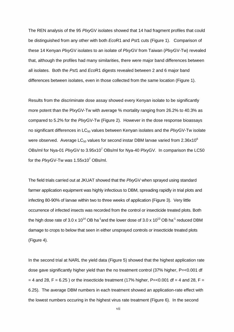
The REN analysis of the 95 PlxyGV isolates showed that 14 had fragment profiles that could

be distinguished from any other with both EcoR1 and Pst1 cuts (Figure 1). Comparison of

these 14 Kenyan PlxyGV isolates to an isolate of PlxyGV from Taiwan (PlxyGV-Tw) revealed

that, although the profiles had many similarities, there were major band differences between

all isolates. Both the Pst1 and EcoR1 digests revealed between 2 and 6 major band

differences between isolates, even in those collected from the same location (Figure 1).

Results from the discriminate dose assay showed every Kenyan isolate to be significantly

more potent than the PlxyGV-Tw with average % mortality ranging from 26.2% to 40.3% as

compared to 5.2% for the PlxyGV-Tw (Figure 2). However in the dose response bioassays

no significant differences in LC50 values between Kenyan isolates and the PlxyGV-Tw isolate

were observed. Average LC50 values for second instar DBM larvae varied from 2.36x106

OBs/ml for Nya-01 PlxyGV to 3.95x107 OBs/ml for Nya-40 PlxyGV. In comparison the LC50

for the PlxyGV-Tw was 1.55x107 OBs/ml.

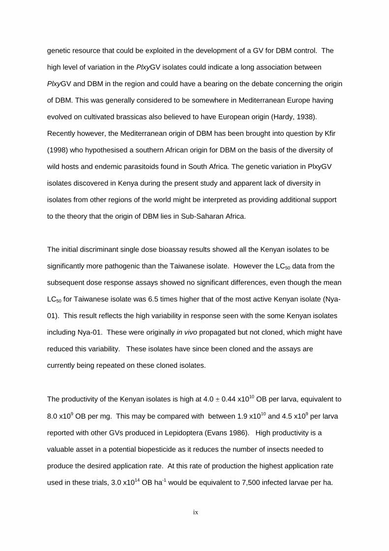
The field trials carried out at JKUAT showed that the PlxyGV when sprayed using standard

farmer application equipment was highly infectious to DBM, spreading rapidly in trial plots and

infecting 80-90% of larvae within two to three weeks of application (Figure 3). Very little

occurrence of infected insects was recorded from the control or insecticide treated plots. Both

the high dose rate of 3.0 x 1014 OB ha-1and the lower dose of 3.0 x 1013 OB ha-1 reduced DBM

damage to crops to below that seen in either unsprayed controls or insecticide treated plots

(Figure 4).

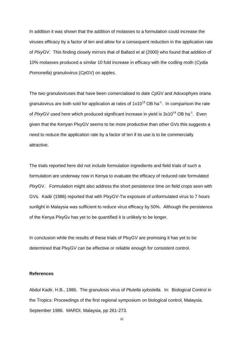
In the second trial at NARL the yield data (Figure 5) showed that the highest application rate

dose gave significantly higher yield than the no treatment control (37% higher, P=<0.001 df

= 4 and 28, F = 6.25 ) or the insecticide treatment (17% higher, P=<0.001 df = 4 and 28, F =

6.25). The average DBM numbers in each treatment showed an application-rate effect with

the lowest numbers occuring in the highest virus rate treatment (Figure 6). In the second

viii

trial average observed DBM infection rates in virus treated plots also showed a clear

application-rate trend with the highest dose producing an average of 40% (Figure 7). In this

trial there was some infection observed in the control and insecticide plots. From insects

sampled from the PlxyGV application-rate plots, the true infection rate was much higher than

that observed in the field and Table 1 shows the percent virus mortality recorded from

insects taken from the plot treated at 3 x1013 OB ha-1.

The maximum productivity of the PlxyGV was found to be 4.0 0.44 x1010 OB per larva

obtained from 2nd instars inoculated with 2.0 x108 OB ml-1.

Discussion

The Pathogen survey revealed that the GV of DBM occurred on 50% of the farms surveyed

though in all cases with a relatively low incidence. On no farm were widespread epizootics

observed or reported by local farmers questioned. The discovery of so many different

genetic isolates (14) in the small number of infected larvae collected is therefore striking.

Previously reported work (Kadir et al 1999) has characterised only two genetically distinct

isolates one from China and one from Taiwan. Other studies of DBM pathogens have also

only reported finding a single genetically distinct isolate from India (Rabindra 1997) and

Japan (Yamada & Yamaguchi 1985).

The GV isolates from Kenya are genetically similar to, though genetically distinct from the

previously reported Taiwanese isolate. This isolate we now know is itself similar to and

closely related to the Chinese isolate (Kadir and Payne 1999). The two isolates studied

differed by 1-3 major bands in the EcoR1, BamH1 and HindIII profiles from each other. The

differences in the Kenyan isolates studied here were greater at 2-6 bands with only two

profiles EcoR1 and Pst1, even amongst isolates collected from the same farm. This genetic

diversity amongst isolates of PlxyGV from Kenya could be extremely useful as a diverse

ix

genetic resource that could be exploited in the development of a GV for DBM control. The

high level of variation in the PlxyGV isolates could indicate a long association between

PlxyGV and DBM in the region and could have a bearing on the debate concerning the origin

of DBM. This was generally considered to be somewhere in Mediterranean Europe having

evolved on cultivated brassicas also believed to have European origin (Hardy, 1938).

Recently however, the Mediterranean origin of DBM has been brought into question by Kfir

(1998) who hypothesised a southern African origin for DBM on the basis of the diversity of

wild hosts and endemic parasitoids found in South Africa. The genetic variation in PlxyGV

isolates discovered in Kenya during the present study and apparent lack of diversity in

isolates from other regions of the world might be interpreted as providing additional support

to the theory that the origin of DBM lies in Sub-Saharan Africa.

The initial discriminant single dose bioassay results showed all the Kenyan isolates to be

significantly more pathogenic than the Taiwanese isolate. However the LC50 data from the

subsequent dose response assays showed no significant differences, even though the mean

LC50 for Taiwanese isolate was 6.5 times higher that of the most active Kenyan isolate (Nya-

01). This result reflects the high variability in response seen with the some Kenyan isolates

including Nya-01. These were originally in vivo propagated but not cloned, which might have

reduced this variability. These isolates have since been cloned and the assays are

currently being repeated on these cloned isolates.

The productivity of the Kenyan isolates is high at 4.0 0.44 x1010 OB per larva, equivalent to

8.0 x109 OB per mg. This may be compared with between 1.9 x1010 and 4.5 x109 per larva

reported with other GVs produced in Lepidoptera (Evans 1986). High productivity is a

valuable asset in a potential biopesticide as it reduces the number of insects needed to

produce the desired application rate. At this rate of production the highest application rate

used in these trials, 3.0 x1014 OB ha-1 would be equivalent to 7,500 infected larvae per ha.

x

In comparison most existing commercial baculovirus products are applied at rates of

between 50-500 larval equivalents per ha (Moscardi 1999).

The first field trial showed that application of PlxyGV at 3x1013 OB ha-1 could reduce DBM

damage much better than either the use of the standard chemical insecticide or the no

treatment control. The very limited effectiveness of the standard insecticide lamda-

cyhalothrin was a finding suggesting significant resistance in DBM. This has since been

confirmed by other work in Kenya (J Cooper 2001) and is now no longer recommended for

DBM control.

The speed with which weekly sprays of PlxyGV initiated infection rates of 90% could indicate

that one or two applications of PlxyGV at the start of the season might be sufficient to start

an epizootic infection in resident DBM populations. However whether augmentative

approach alone would be sufficient to produce control of DBM numbers and damage though

would need testing under field conditions. While collection of a high percentage of infected

insects in virus treated plots suggests that recycling of PlxyGV is very important its precise

contribution to control remains to be quantified.

In the second trial the yield results showed that again the PlxyGV performed significantly

better than the chemical insecticide at the highest application rate used 3x1014 OB ha-1. A

similar result in terms of controlling DBM numbers has been reported previously by Su

(1989) using a Taiwanese isolate applied as here at seven day intervals. However direct

comparisons are difficult, as in that trial the PlxyGV was quantified in terms of larval

equivalents per litre and no direct enumeration of the GV was carried out.

Glasshouse trials again have showed that application of the Taiwanese isolate can reduce

DBM numbers and that there is a dose response over the range 9 x1011 to 9x1013 and at the

highest dose the PlxyGV reduced damage as effectively as application of Bt (Kadir 1992).

xi

In addition it was shown that the addition of molasses to a formulation could increase the

viruses efficacy by a factor of ten and allow for a consequent reduction in the application rate

of PlxyGV. This finding closely mirrors that of Ballard et al (2000) who found that addition of

10% molasses produced a similar 10 fold increase in efficacy with the codling moth (Cydia

Pomonella) granulovirus (CpGV) on apples.

The two granuloviruses that have been comercialised to date CpGV and Adoxophyes orana

granulovirus are both sold for application at rates of 1x1013 OB ha-1. In comparison the rate

of PlxyGV used here which produced significant increase in yield is 3x1014 OB ha-1. Even

given that the Kenyan PlxyGV seems to be more productive than other GVs this suggests a

need to reduce the application rate by a factor of ten if its use is to be commercially

attractive.

The trials reported here did not include formulation ingredients and field trials of such a

formulation are underway now in Kenya to evaluate the efficacy of reduced rate formulated

PlxyGV. Formulation might also address the short persistence time on field crops seen with

GVs. Kadir (1986) reported that with PlxyGV-Tw exposure of unformulated virus to 7 hours

sunlight in Malaysia was sufficient to reduce virus efficacy by 50%. Although the persistence

of the Kenya PlxyGv has yet to be quantified it is unlikely to be longer.

In conclusion while the results of these trials of PlxyGV are promising it has yet to be

determined that PlxyGV can be effective or reliable enough for consistent control.

References

Abdul Kadir, H.B., 1986. The granulosis virus of Plutella xylostella. In: Biological Control in

the Tropics: Proceedings of the first regional symposium on biological control, Malaysia.

September 1986. MARDI, Malaysia, pp 261-273.

xii

Abdul Kadir, H.B. (1990). Potential of several baculoviruses for the control of diamondback

moth and Crocidolomia binotalis on cabbages. In: “Diamondback moth and other crucifer

pests”, proceedings of the second international workshop, Tainan, Taiwan, 10-14 December

1990, N. S. Talekar, (ed), pp 185-192.

Abdul Kadir, H.B., 1992. Potential of several baculoviruses for the control of diamondback

moth and Crocidolomia binotalis on cabbages. In : Talekar, N.S. (Ed), Diamondback Moth

and Other Crucifer Pests. Proceedings of the Second International Workshop, Tainan,


Abdul Kadir, H.B., Payne, C.C., Crook, N.E., and Winstanley, D. 1999. Characterization and

cross-transmission of baculoviruses infective to the diamondback moth, Plutella xylostella,

and some other Lepidopterous pests of brassica crops. Biocontrol Sci. Technol. 9, 227-238.

Asayama, T. and Osaki, N. 1970. A granulosis of the diamondback moth, Plutella


Ballard J Ellis D J and Payne C C (2000) The role of formulation additives in increasing the

potency of Cydia pomonella granulovirus for coddling moth larvae in laboratory and field

experiments. Biocontrol Science and technology 10:627-640.

Cooper J (2001) Pest management in horticultural crops: an integrated approach to

vegetable pest management with the aim of reducing reliance on pesticides in Kenya. NRI

Final Technical Report R7403, pp36.

Copping L (1998) The Biopesticides Manual. BCPC Publications, Bracknell

xiii

Hardy, J.E., 1938. Plutella maculipennis Curt. Its natural and biological control in England.

Bull. of Entomol. Res. 29, 343-372.

Kfir, R., 1998. Origin of the diamondback moth (Lepidoptera: Plutellidae). Annals of the

Entomological Society of America, 91, (2), 164-167.




Jenkins, N. E. and D. Grzywacz. 2000. Quality control-assurance of product performance.

Biocontrol Science and Technology, 10, 753-777.

Kibata, G.N. 1997. The diamondback moth: A problem pest of brassica crops in Kenya. In



Workshop, Kuala Lumpur, Malaysia 29 October - 1 November, 1996. MARDI, Malaysia, pp

47-53.

Lisansky, S. (1997) Microbial biopesticides. In Microbial Insecticides: Novelty or Necessity?

British Crop Protection Council Proceeding Monograph Series No 68. pp. 3-10.




Moscardi, F. (1999) Assessment of the application of baculoviruses for control of

Lepidoptera. Annual Review of Entomology 44, 257-289.

xiv

Oruku L and Ndun’gu B (2001) Final socio-economic Report for the peri-urban vegetable

IPM thematic cluster. CABI Africa Regional Centre Report, Nairobi, pp49.

Padmavathamma, K. and Vereesh, G.K., 1989. Effect of contamination of eggs of the

diamondback moth, Plutella xylostella (Linnaeus) with nuclear polyhedrosis virus. J. Biol.

Cont. 3, 73-74.

Parnell, M. A., 1999. The genetic variability and efficacy of baculoviruses for control of

diamondback moth on brassica vegetables in Kenya. MSc Thesis, University of Greenwich,

Greenwich, UK. pp 72.

Rabindra, R.J., Geetha, N., Renuka, S., Varadharajan, S., Regupathy, A., 1997. Occurrence

of a granulosis virus from two populations of Plutella xylostella (L.) in India. In:




113-115.

Roush, T. 1997. Insecticide resistance management in diamondback moth: quo vadis? In




21-24.

Smith, G.E. and Summers, M.D. 1978. Analysis of baculovirus genomes with restriction


xv

Su, C.Y., 1989. The evaluation of granulosis viruses for control of three lepidopterous insect

pests on cruciferous vegetables. Chin. J. Entomol. 9, 189-196.

Tabashnik, B.E., 1994. Evolution of resistance to Bacillus thuringiensis. Ann. Rev. Entomol.

39, 47-79.

Wilding N (1986) Pathogens of diamond back moth and their potential for its control a review.

pp219-232

Wright D J Iqbal M Verkerk H J (1995) Resistance to Bacillus thuringiensis and abermectin in

the diamondback moth Plutella xylostella: A major problem for Integrated pest management

Med.Fac. Landouww Univ Ghent 60 3b 927-932

Yamada, H. and Yamaguchi, T., 1985. Notes on parasites and predators attacking the

diamondback moth, Plutella xylostella. Japenese J. Appl. Entomol. and Zool. 29 (2), 170-

173.

xvi

AN APPRAISAL OF THE PHEROMONE MATING-DISRUPTION

TECHNIQUE FOR MANAGEMENT OF DIAMOND-BACK MOTH,

PLUTELLA XYLOSTELLA

xvii

AN APPRAISAL OF THE PHEROMONE MATING-DISRUPTION

TECHNIQUE FOR MANAGEMENT OF DIAMOND-BACK MOTH,

PLUTELLA XYLOSTELLA

A Technical Report for Project R7449:

Development of Biorational Brassica IPM in Kenya

DFID Crop Protection Programme

M.C.A. Downham

Natural Resources Institute, Medway University Campus, University of

Greenwich, Chatham, Kent ME4 4TB, United Kingdom

Collaborating Institutions:

Natural Resources Institute, UK

KARI, National Agricultural Research Laboratories, Kenya

CABI International, Africa Regional Centre, Kenya

xviii

Contents

Executive Summary 1

Acknowledgements 2

Introduction 3

Materials and Methods 6

Location of trial sites 6

Crops and agronomic practices 6

Plot sizes and treatments 7

Monitoring and evaluation of treatments 8

Duration of the trial 9

Data analysis 9

Results 12

Pheromone trap catches 12

Weekly DBM counts 14

Non DBM counts 16

Harvests 18

Quantitative analysis of Selibate dispensers 19

Discussion 21

The present results 21

Pest incidence 21

Resurgence effects 22

Use of 'buffer zones' 23

Other mating-disruption studies with DBM 23

Limitations of the methods used in the 2000 trials 25

Conclusions 27

Specific Recommendations for a Further Trial 28

References 29

Appendices 33

1

Executive Summary

A trial of pheromone mating disruption of diamondback moth (DBM), Plutella xylostella, L.

was carried out at three sites near Nairobi, Kenya from March to August 2000. The synthetic

pheromone formulation used was a PVC-based one known as 'Selibate' and individual

dispensers were set out at a density of approximately 625 ha-1

. At each site single, 0.1 ha

plots of kale containing 60 and 120 g ha-1

of pheromone active ingredient were compared

with a control plot. One or two aphicide sprays were made early in the season in all plots, but

controls were otherwise untreated. As determined by weekly sampling, populations of pests,

including DBM, were low throughout the trial and no clear between-treatment differences in

the numbers of DBM larvae and pupae, or in yield, were observed. Pheromone trap

monitoring indicated incomplete suppression of catches in the pheromone-treated plots, even

in the early stages of the trial, when disruption of pheromone-mediated behaviour should

have been greatest. From the results it is concluded that the pheromone treatments did not

disrupt mating of DBM. It is concluded that previous, apparently successful, results in Kenya

may have been due to insecticide 'resurgence' effects in control plots providing a favourable,

but misleading, comparison with the pheromone plots. Through a comparison of trial results

from elsewhere, it is further concluded that the only chance of successful mating disruption in

the Kenyan, small-holder farmer context lies in increasing pheromone dispenser density and

effective plot size (through the use of 'buffer zones'). Accordingly, recommendations are

made for a trial incorporating these and other changes.

2

Acknowledgements

I am greatly indebted to the unstinting efforts of Dr G. Oduor and Mr W. Okello Ogutu from

CABI-ARC and Dr G.N. Kibata and Mr D. Miano of KARI who set-up and managed the trial

at the three field sites. The respective field teams from both organisations worked tirelessly

throughout the long trial period. I am grateful for the assistance of Mr Wanyonyi (Irrigation

Manager) and Mr Mbuvi (Farm Manager) at the University of Nairobi farm, Kabete.

Similarly, Mr Kaibui (Assistant Farm Manager) at Jomo Kenyatta University of Agriculture

and Technology was immensely helpful in managing the trial plots there, as were numerous

colleagues at Ongata Rongai farm. I thank the following NRI staff members: Mark Parnell

for assistance in finding the trial sites, Dr David Jeffries for his statistical advice, Mrs

Margaret Brown for procurement assistance, and Dudley Farman for laboratory analysis of

mating disruption dispensers.

This publication is an output from project R7449 funded by the Crop Protection Programme

of the United Kingdom Department for International Development (DFID) for the benefit of

developing countries. The views expressed are not necessarily those of DFID.

3

Introduction

Project R7449 aims to develop, evaluate and promote two new biologically based IPM

control methods for the diamond-back moth (DBM), Plutella xylostella, L. on small-holder

vegetable farms in Kenya. These are the use of pheromone-based mating-disruption and an

endemic viral bio-pesticide. This report concerns trials to develop the first of these. It has

two main objectives: to report detailed results from trials carried out in the 2000 and to

discuss these in the context of earlier trials in Kenya during the previous project phase

(R6615) (Critchley et al., 1998, 1999a, 1999b) and, elsewhere, by others.

The technique of mating-disruption involves the release of pheromone within a crop, such

that mate location is disrupted or impaired in some way, and subsequent infestations reduced

or eliminated. As in the present case - with brassica crops in peri-urban Kenya - it has

generally been developed in crops in which insecticide usage is problematic due the

development of resistance, or is undesirable because the product is destined for human

consumption.

Several commercial formulations of pheromone dispenser have been developed for mating-

disruption. All aim to provide a controlled release of pheromone into the crop over a long

period, and protection against chemical degradation as well as ease of application. The

formulation used in the current work is based on a poly-vinyl chloride matrix and was

originally developed at NRI (Cork et al., 1989).

The identity of the sex pheromone of DBM is well established. Many years ago it was shown

to comprise a mixture of three components, principally (Z)-11-hexadecenal (Z11-16:Ald) and

(Z)-11-hexadecenyl acetate (Z11-16:Ac) (Tamaki et al., 1977; Koshihara et al. 1978), with a

small quantity of (Z)-11-hexadecenol (Z11-16:OH) (Ando et al., 1979; Koshihara & Yamada,

1980). The geographic origin of DBM may affect the optimum ratio of blend components.

In Canada a 70:30:1 mixture (of Z11-16:Ald: Z11-16:Ac: Z11-16:OH) appears best

(Chisholm et al., 1979; Chisholm et al., 1983) but in Japan 50:50:1 is more effective

(references above; Kawasaki, 1984). It was assumed at the outset of the previous project

R6615 that the race of DBM in Kenya would more closely resemble that in Asia than that in

America (Critchley et al., 1998). Therefore the 50:50:1 blend was adopted as standard.

4

The studies by Critchley and colleagues in Kenya took place against a background of several

previous successful trials of mating-disruption of DBM. In Japan, Ohbayashi et al. (1992),

and to a lesser degree Nemoto et al. (1992), found large reductions in catches of males in

monitoring traps in plots, lower rates of mating and reduced larval numbers in pheromone

treated brassica and vegetable plots, compared with untreated or insecticide treated fields.

Similarly, on commercial cabbage farms in Florida, USA McLaughlin et al. (1994) and

Mitchell et al. (1997) obtained good control of the pest in pheromone plots compared to

fields treated with insecticides. With the exception of that by Nemoto et al. (1992) all these

studies had used relatively high ( 250 g ha-1

) rates of application of the pheromone active

ingredient that could not be considered economically viable (Talekar & Shelton, 1993). All

were carried out in fields of several hectares or more. Therefore these trials could not be

regarded as realistic in terms of the constraints faced by small-holder farmers in Africa. Ohno

et al. (1992), in Japan, and Schroeder et al. (2000) in the USA have carried out trials in much

smaller, 0.1 and 0.2 ha plots, respectively (though also with application rates of at least 250 g

ha-1

), but these yielded conflicting results.

In this context, for work in Kenya it was important to investigate the possibility of mating-

disruption of DBM in small plots, typical of those cultivated by Kenyan small-holder

farmers, using lower rates of application that were more likely to be economically viable.

Work on the previous project phase was carried out in the major rainy seasons of 1997 (May

- July) and 1998 (May - September), and the major dry season of 1999 (February - April).

During the first year much of the work consisted of identifying the most practical traps and

lures to be used in subsequent work (Critchley et al., 1998). Results obtained then dictated

the trap and lure types used since then (see Materials and Methods). Two further sets of

preliminary observations provided encouraging indications of the feasibility of mating-

disruption under Kenyan conditions. Mating-disruption dispensers placed in 12 × 12 m plots

depressed catches by traps in the centre of the plots by 73 - 98%, compared to untreated plots,

10 weeks after application, indicating that males' ability to locate individual pheromone

sources within small treated areas was greatly reduced over this period. Furthermore,

measurements of the persistence of the pheromone in the mating-disruption dispensers

showed that most (60 - 70%) remained after two months exposure under field conditions.

5

In 1998 and 1999 full-scale trials were undertaken in kale crops. In 1998, dispensers were set

out in 0.1 ha plots and in 4 - 8 m wide buffer zones around each plot. The density of sources

was varied between each of three sites, but by also varying the amount of pheromone within

individual dispensers the overall application rate was maintained at approximately 60 g ha-1

.

Pheromone plots were compared to controls that were intended to be representative of typical

farmer practice. Consequently, the latter received several insecticide sprays against DBM

and non-DBM pests. The pheromone treated plots received some limited sprays against non-

DBM pests. In the following year a similar approach was taken. Identical treatment and

control plots were set out at two sites but plots were only 0.05 ha in size, the pheromone plots

lacked buffer zones and the application rate was slightly lower (53 g ha-1

). Mating-disruption

dispensers were placed at the highest and most effective density used in 1998.

In the 1998 trials (Critchley et al. 1999a), the effectiveness of the pheromone treatment

appeared to be positively associated with the density of mating-disruption dispensers. In the

highest source density (625 ha-1

) plot, trap catches of males were completely suppressed for

more than 10 weeks after application, larval and pupal numbers and plant damage scores

were consistently much lower, relative to the control, and total marketable yield was double

that of the control plot. There was no evidence of any controlling effect at the lowest density

of pheromone dispensers (156 ha-1

), while results for the medium density (312 ha-1

) plot were

intermediate in most respects. In 1999, the effectiveness of the pheromone treatment was

much less marked than for comparable results in 1998. At one site complete trap catch

suppression was never achieved, and larval numbers and plant damage scores were usually

only slightly lower than in control plots, if at all. Nevertheless yield in the pheromone plot

was substantially greater at one site; no valid yield data were available at the second site

(Critchley et al. 1999b).

6

Materials and Methods

Location of trial sites

The trial was conducted at three sites: the University of Nairobi farm at Kabete, about 6 km

north-west of Nairobi; the Jomo Kenyatta University of Agriculture and Technology farm site

(JKUAT), situated about 24 km north-east of Nairobi; a small commercial farm at Ongata

Rongai, approximately 20 km south-west of Nairobi.

Crops and agronomic practices

The target crop was kale (Collard var. Southern Georgia), Brassica oleracea. All plants were

transplanted into the plots as seedlings with 3 – 6 true leaves at a spacing of 60 60 cm.

Seedlings used at Kabete and JKUAT came from nursery beds at KARI/NARL (from screen-

house and field beds respectively). Those used at Ongata Rongai came from a local

commercial nursery. Transplanting at Kabete, JKUAT and Ongata Rongai took place on 10,

14 and 21 March 2000, respectively. Due to dry weather all plots were irrigated, manually or

using overhead irrigation equipment, for at least two weeks following transplanting, and

thereafter were rain-fed. Despite this, quite large numbers of seedlings died, necessitating

gap-filling. This was most severe at Kabete where up to half of the seedlings needed to be

replanted 1 – 2 weeks after initial transplanting.

Fertiliser applications and weeding were carried out as indicated in Table 1 below. DAP was

applied at planting while CAN was a top dressing at a rate 5 g and 10 g per plant respectively.

Table 1. Dates of fertiliser applications and weeding at the three trial sites.

Operation Kabete JKUAT Ongata Rongai

Fertiliser

applications

10 March 14 March 21 March

5 April 5 April and 12 June 11 April

Weeding 28 March 4 April 10 April

27 April 18 April 27 April

14 June 10 May 24 May

26 July 14 June 21 June

10 July 20 July

7

Early season insecticide applications were made against aphids (mainly Brevicoryne

brassicae) using aphid-specific products. All plots at Ongata Rongai and Kabete received two

sprays, and those at JKUAT one spray. Sprays at Ongata Rongai and Kabete on 4 April 2000

used Pymetrozine 50 WG (200 g in 500 l water ha-1

), a novel product from Novartis. At

JKUAT on 5 April and at Ongata Rongai and Kabete on 2 – 3 May, sprays were made with

Pirimor 50 WP (Pirimicarb, 250 g in 500 l water ha-1

).

Plot sizes and treatments

Individual plots were 0.09 - 0.10 ha in area; dimensions varied from 30 30 m to 20 50 m.

Plots were situated at least 50 m apart to minimise the effect of pheromone dispensers in one

plot on others. At Kabete and Ongata Rongai plots were at least 100 m from other brassica

crops which might act as sources of infestation, but at JKUAT one end of the plots was only

10 m from another field of kale.

Three plots were planted at each site: an untreated control, a pheromone treatment of

approximately 60 g a.i. ha-1

and one of 120 g a.i. ha-1

. For both pheromone treatments the

formulation used was a black, PVC „shoelace‟ or Selibate™ formulation (Cork et al., 1989)

produced by Agrisense-BCS, Pontypridd, UK in December 1999. This contained a blend of

(Z)-11-hexadecenal, (Z)-11-hexadeceny acetate and (Z)-11-hexadecenol in the ratio 30:30:1,

with a total active ingredient content of 7.9 mg g-1

(determined by analysis at NRI). The

departure of the blend from the nominal 50:50:1 ratio was not considered to be biologically

significant. The differences in application rate of the pheromone treatments were achieved

by applying different amounts of the formulation; lengths weighing 1 or 2 g were used.

These treatments are hereafter referred to as the 1g and 2g pheromone treatments,

respectively.

Individual lengths of the formulation were fixed into the split top end of bamboo canes, at a

height of 1 m, and applied 4 m apart in a grid pattern (approximating 625 ha-1

), the day after

transplanting (Figs. 1 and 2). Due to differing plot dimensions the number of dispensers per plot

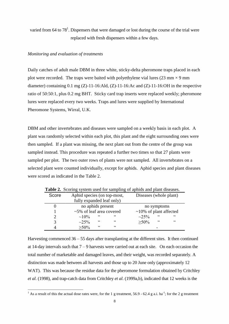
8

varied from 64 to 781. Dispensers that were damaged or lost during the course of the trial were

replaced with fresh dispensers within a few days.

Monitoring and evaluation of treatments

Daily catches of adult male DBM in three white, sticky-delta pheromone traps placed in each

plot were recorded. The traps were baited with polyethylene vial lures (23 mm × 9 mm

diameter) containing 0.1 mg (Z)-11-16:Ald, (Z)-11-16:Ac and (Z)-11-16:OH in the respective

ratio of 50:50:1, plus 0.2 mg BHT. Sticky card trap inserts were replaced weekly; pheromone

lures were replaced every two weeks. Traps and lures were supplied by International

Pheromone Systems, Wirral, U.K.

DBM and other invertebrates and diseases were sampled on a weekly basis in each plot. A

plant was randomly selected within each plot, this plant and the eight surrounding ones were

then sampled. If a plant was missing, the next plant out from the centre of the group was

sampled instead. This procedure was repeated a further two times so that 27 plants were

sampled per plot. The two outer rows of plants were not sampled. All invertebrates on a

selected plant were counted individually, except for aphids. Aphid species and plant diseases

were scored as indicated in the Table 2.

Table 2. Scoring system used for sampling of aphids and plant diseases.

Score Aphid species (on top-most,

fully expanded leaf only)

Diseases (whole plant)

0 no aphids present no symptoms

1 ~5% of leaf area covered ~10% of plant affected

2 ~10% “ “ ~25% “ “

3 ~25% “ “ ≥50% “ “

4 ≥50% “ “ -

Harvesting commenced 36 – 55 days after transplanting at the different sites. It then continued

at 14-day intervals such that 7 – 9 harvests were carried out at each site. On each occasion the

total number of marketable and damaged leaves, and their weight, was recorded separately. A

distinction was made between all harvests and those up to 20 June only (approximately 12

WAT). This was because the residue data for the pheromone formulation obtained by Critchley

et al. (1998), and trap-catch data from Critchley et al. (1999a,b), indicated that 12 weeks is the

1 As a result of this the actual dose rates were, for the 1 g treatment, 56.9 - 62.4 g a.i. ha

-1; for the 2 g treatment

9

approximate half-life of the formulation, and is probably the maximum period over which trap-

catches in treated plots are suppressed. Together these suggested that any impact on yield

should be confined to the first 12 weeks after transplanting. In each plot the initial (after gap-

filling) and final (after last harvest) plant stand was also determined.

Quantitative analysis of the mating-disruption formulation was also carried out. Five lengths

were retrieved from each treated plot at each site on 8 August 2000 (140 – 151 days after

transplanting), wrapped in aluminium foil and refrigerated before being sent back to NRI for

analysis. The amount of each pheromone component contained in three sub-sample lengths of

the formulation from each plot was then determined and compared to un-exposed samples taken

from the packet supplied on 23 March.

Duration of the trial

The original intention was for the trial to last 12 – 15 weeks. However generally low

populations of DBM resulted in the decision to leave the crop in the ground, and monitoring to

continue, until about 19 weeks after planting, in the hope of encountering sufficiently large

populations that between-treatment differences might become apparent.

Data analysis

In the present design there is no suitable method of statistical comparison of monitoring data or

sample harvests, as the geographically separate sites cannot be regarded as replicate blocks (D.

Jeffries, pers. comm.). This is because the size of any treatment × block interactions cannot be

estimated (there was only one replicate of each treatment per site). However, large or temporally

consistent differences between data from different plots, may be considered as indicative of real

differences.

they were 113.8 - 124.8 g a.i. ha-1

.

10

Figure 1. Selibate™ DBM mating-disruption dispenser fixed into bamboo cane.

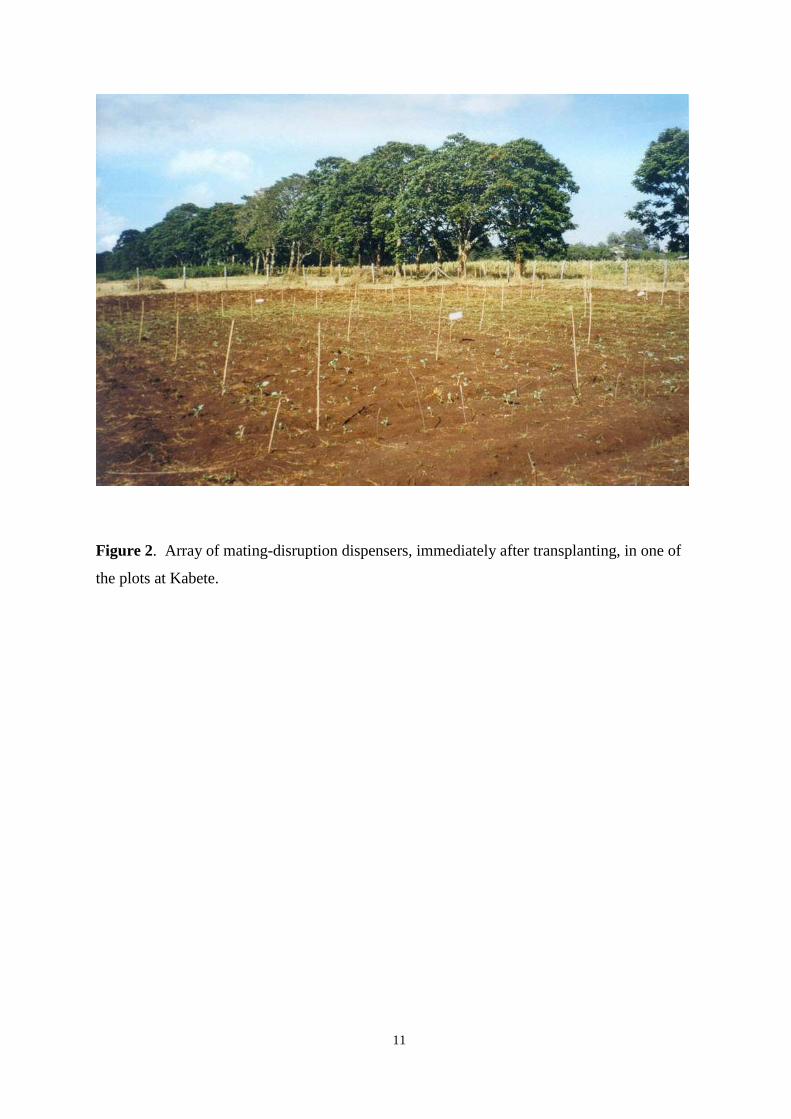
11

Figure 2. Array of mating-disruption dispensers, immediately after transplanting, in one of

the plots at Kabete.

12

Results

Pheromone trap catches

Catches of male DBM adults were nearly always highest in control plots, especially at the

start of the season (Figs. 3 - 5). The difference between catches in the control and pheromone

plots tended to decrease through the trial period, so that they were similar in the last few

weeks. The relative magnitude of catches in the control and pheromone plots are illustrated in

Table 3. General catch levels fluctuated through the season, but trends differed between sites.

Peak catches of 20 - 22 male DBM adults per week were reached in control plots at Kabete

18 - 20 WAT and at JKUAT from 3 - 9 WAT (Figs. 3 and 4). Those at Ongata Rongai

occurred from 9 - 15 WAT, and were less than half as great (Fig. 5).

Figure 3. Mean weekly trap-catch results for Kabete (means of 3 traps for each plot).

0

5

10

15

20

25

1 2 3 4 5 6 7 8 9 10 11 12 13 14 15 16 17 18 19 20 21

Weeks after transplanting

Me

an

mo

ths

/tra

p/w

ee

k

2 g

1 g

control

13

Figure 4. Mean weekly trap-catch results for JKUAT (means of 3 traps for each plot).

Figure 5. Mean weekly trap catches at Ongata Rongai (means of 3 traps for each plot).

0

5

10

15

20

25

1 2 3 4 5 6 7 8 9 10 11 12 13 14 15 16 17 18 19 20 21


Me

an

ca

tch

/tra

p/w

ee

k

2 g

1 g

control

0

2

4

6

8

10

1 2 3 4 5 6 7 8 9 10 11 12 13 14 15 16 17 18 19 20


Me

an

ca

tch

/tra

p/w

ee

k

2 g

1 g

control

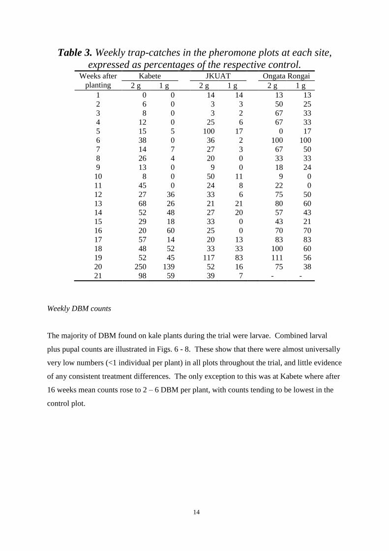
14

Table 3. Weekly trap-catches in the pheromone plots at each site,

expressed as percentages of the respective control. Weeks after

planting

Kabete JKUAT Ongata Rongai

2 g 1 g 2 g 1 g 2 g 1 g

1 0 0 14 14 13 13

2 6 0 3 3 50 25

3 8 0 3 2 67 33

4 12 0 25 6 67 33

5 15 5 100 17 0 17

6 38 0 36 2 100 100

7 14 7 27 3 67 50

8 26 4 20 0 33 33

9 13 0 9 0 18 24

10 8 0 50 11 9 0

11 45 0 24 8 22 0

12 27 36 33 6 75 50

13 68 26 21 21 80 60

14 52 48 27 20 57 43

15 29 18 33 0 43 21

16 20 60 25 0 70 70

17 57 14 20 13 83 83

18 48 52 33 33 100 60

19 52 45 117 83 111 56

20 250 139 52 16 75 38

21 98 59 39 7 - -

Weekly DBM counts

The majority of DBM found on kale plants during the trial were larvae. Combined larval

plus pupal counts are illustrated in Figs. 6 - 8. These show that there were almost universally

very low numbers (<1 individual per plant) in all plots throughout the trial, and little evidence

of any consistent treatment differences. The only exception to this was at Kabete where after

16 weeks mean counts rose to 2 – 6 DBM per plant, with counts tending to be lowest in the

control plot.

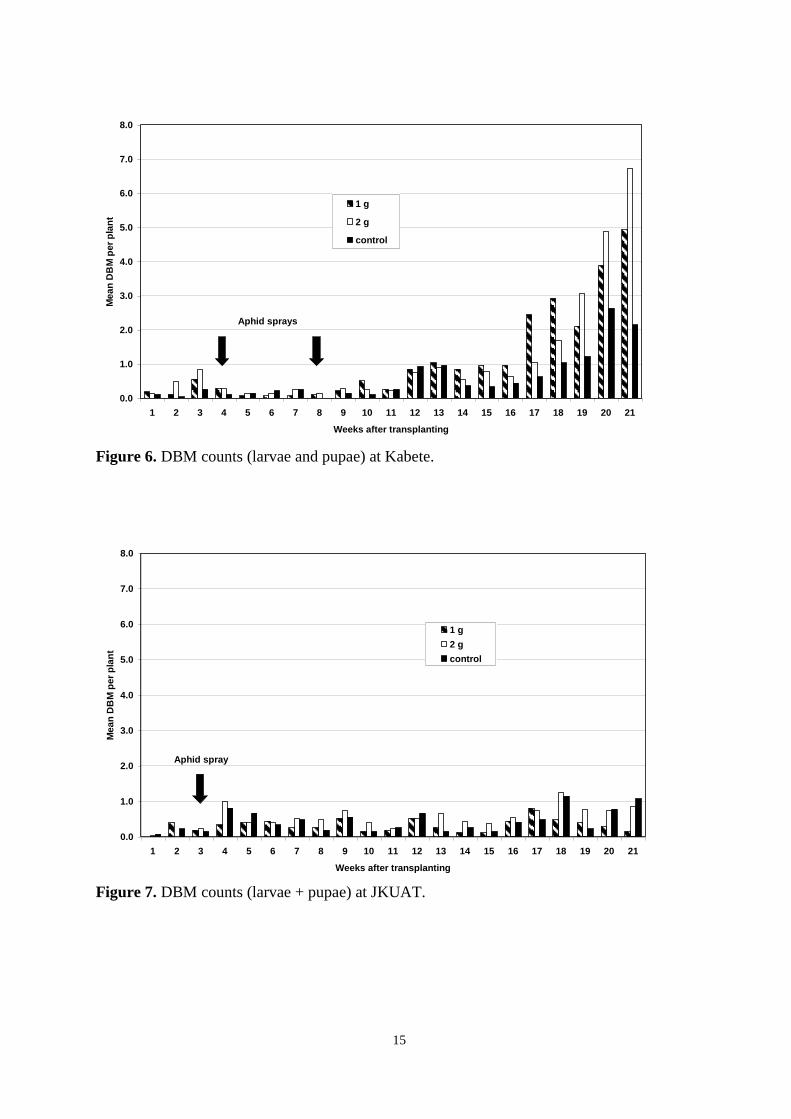
15

Figure 6. DBM counts (larvae and pupae) at Kabete.

Figure 7. DBM counts (larvae + pupae) at JKUAT.

0.0

1.0

2.0

3.0

4.0

5.0

6.0

7.0

8.0

1 2 3 4 5 6 7 8 9 10 11 12 13 14 15 16 17 18 19 20 21


Me

an

DB

M p

er

pla

nt

1 g

2 g

control

Aphid spray

0.0

1.0

2.0

3.0

4.0

5.0

6.0

7.0

8.0

1 2 3 4 5 6 7 8 9 10 11 12 13 14 15 16 17 18 19 20 21


Me

an

DB

M p

er

pla

nt

1 g

2 g

control

Aphid sprays

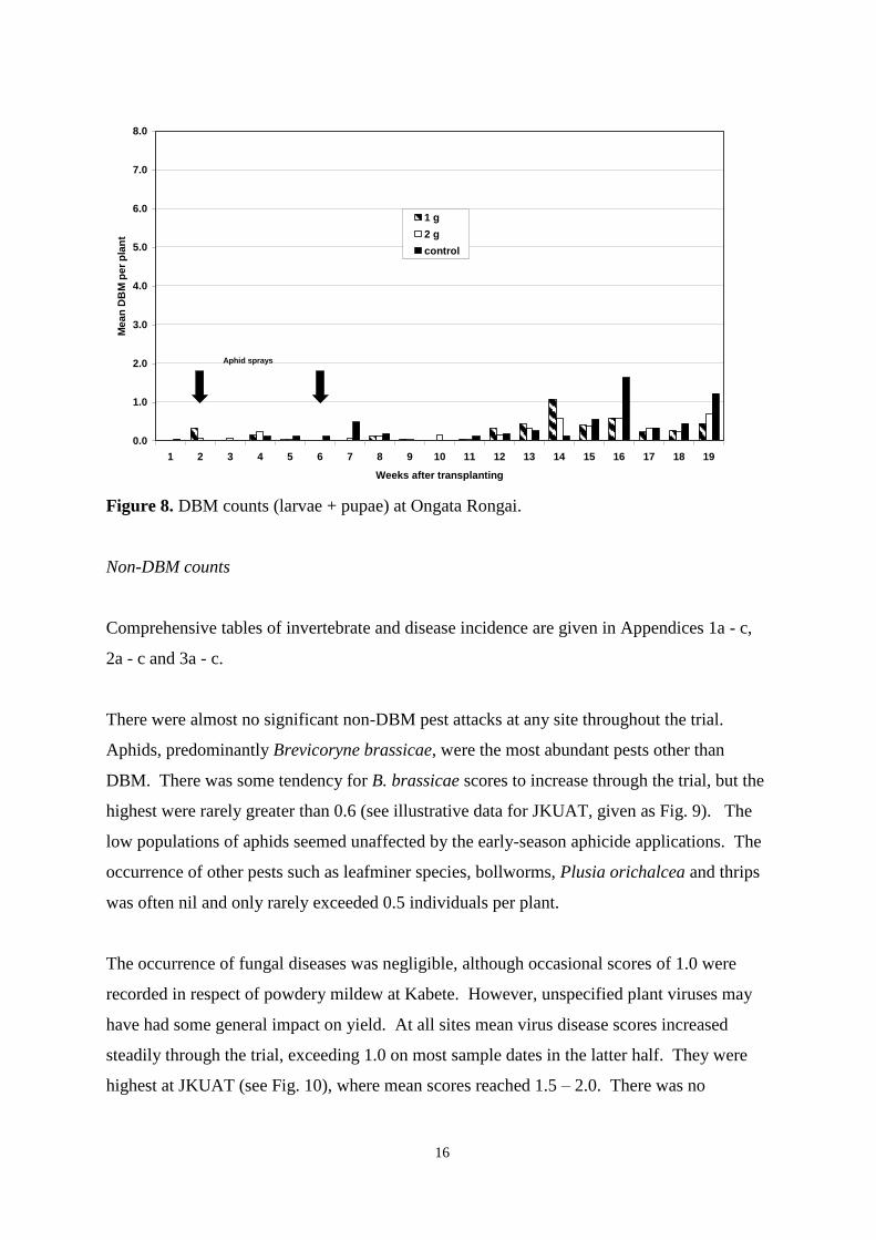
16

Figure 8. DBM counts (larvae + pupae) at Ongata Rongai.

Non-DBM counts

Comprehensive tables of invertebrate and disease incidence are given in Appendices 1a - c,

2a - c and 3a - c.

There were almost no significant non-DBM pest attacks at any site throughout the trial.

Aphids, predominantly Brevicoryne brassicae, were the most abundant pests other than

DBM. There was some tendency for B. brassicae scores to increase through the trial, but the

highest were rarely greater than 0.6 (see illustrative data for JKUAT, given as Fig. 9). The

low populations of aphids seemed unaffected by the early-season aphicide applications. The

occurrence of other pests such as leafminer species, bollworms, Plusia orichalcea and thrips

was often nil and only rarely exceeded 0.5 individuals per plant.

The occurrence of fungal diseases was negligible, although occasional scores of 1.0 were

recorded in respect of powdery mildew at Kabete. However, unspecified plant viruses may

have had some general impact on yield. At all sites mean virus disease scores increased

steadily through the trial, exceeding 1.0 on most sample dates in the latter half. They were

highest at JKUAT (see Fig. 10), where mean scores reached 1.5 – 2.0. There was no

0.0

1.0

2.0

3.0

4.0

5.0

6.0

7.0

8.0

1 2 3 4 5 6 7 8 9 10 11 12 13 14 15 16 17 18 19


Me

an

DB

M p

er

pla

nt

1 g

2 g

control

Aphid sprays

17

indication that disease scores were linked to the presence or absence of pheromone

treatments.

Figure 9. Mean weekly Brevicoryne spp. aphid scores at JKUAT.

Figure 10. Mean weekly plant virus scores at JKUAT.

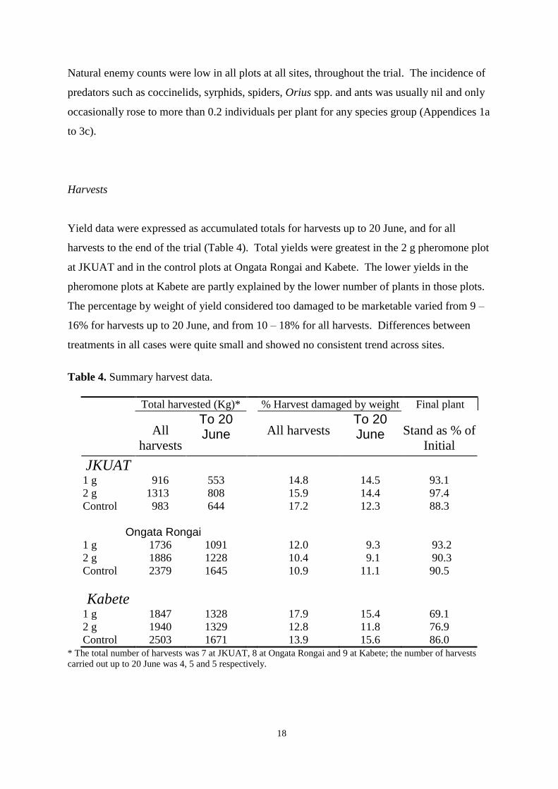
18

Natural enemy counts were low in all plots at all sites, throughout the trial. The incidence of

predators such as coccinelids, syrphids, spiders, Orius spp. and ants was usually nil and only

occasionally rose to more than 0.2 individuals per plant for any species group (Appendices 1a

to 3c).

Harvests

Yield data were expressed as accumulated totals for harvests up to 20 June, and for all

harvests to the end of the trial (Table 4). Total yields were greatest in the 2 g pheromone plot

at JKUAT and in the control plots at Ongata Rongai and Kabete. The lower yields in the

pheromone plots at Kabete are partly explained by the lower number of plants in those plots.

The percentage by weight of yield considered too damaged to be marketable varied from 9 –

16% for harvests up to 20 June, and from 10 – 18% for all harvests. Differences between

treatments in all cases were quite small and showed no consistent trend across sites.

Table 4. Summary harvest data.

Total harvested (Kg)* % Harvest damaged by weight Final plant

All

harvests

To 20 June All harvests

To 20 June Stand as % of

Initial

JKUAT

1 g 916 553 14.8 14.5 93.1

2 g 1313 808 15.9 14.4 97.4

Control 983 644 17.2 12.3 88.3

Ongata Rongai

1 g 1736 1091 12.0 9.3 93.2

2 g 1886 1228 10.4 9.1 90.3

Control 2379 1645 10.9 11.1 90.5

Kabete

1 g 1847 1328 17.9 15.4 69.1

2 g 1940 1329 12.8 11.8 76.9

Control 2503 1671 13.9 15.6 86.0 * The total number of harvests was 7 at JKUAT, 8 at Ongata Rongai and 9 at Kabete; the number of harvests

carried out up to 20 June was 4, 5 and 5 respectively.

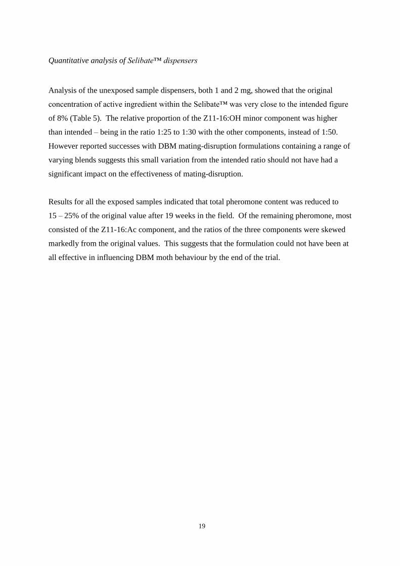
19

Quantitative analysis of Selibate™ dispensers

Analysis of the unexposed sample dispensers, both 1 and 2 mg, showed that the original

concentration of active ingredient within the Selibate™ was very close to the intended figure

of 8% (Table 5). The relative proportion of the Z11-16:OH minor component was higher

than intended – being in the ratio 1:25 to 1:30 with the other components, instead of 1:50.

However reported successes with DBM mating-disruption formulations containing a range of

varying blends suggests this small variation from the intended ratio should not have had a

significant impact on the effectiveness of mating-disruption.

Results for all the exposed samples indicated that total pheromone content was reduced to

15 – 25% of the original value after 19 weeks in the field. Of the remaining pheromone, most

consisted of the Z11-16:Ac component, and the ratios of the three components were skewed

markedly from the original values. This suggests that the formulation could not have been at

all effective in influencing DBM moth behaviour by the end of the trial.

Table 5. Summary results of quantitative analysis of DBM Selibate formulation; figures are all means of three samples.

Sample Amount of pheromone components

(mg/100 mg formulation)

Total

(mg/100 mg)

Component ratios

Z11-16:Ald Z11-16:Ac Z11-16:OH Ald:Ac Ald:OH Ac:OH

Unexposed 1g 3.83 3.95 0.13 7.91 0.97 29.60 30.49

Unexposed 2g 3.79 3.88 0.16 7.84 0.98 24.09 24.58

JKUAT 1g 0.53 1.44 0.01 1.98 0.36 64.96 178.28

JKUAT 2g 0.05 1.40 0.01 1.46 0.04 7.83 205.75

Kabete 1g 0.23 1.07 0.01 1.31 0.21 21.19 97.44

Kabete 2g 0.12 1.04 0.01 1.17 0.14 10.93 89.35

Ongata Rongai 1g 0.08 2.14 0.01 2.23 0.04 7.82 220.97

Ongata Rongai 2g 0.08 1.83 0.01 1.92 0.04 8.16 205.12

Formulation produced by Agrisense-BCS 22 December 1999; unexposed samples taken from bags 23 March 2000; exposed

samples all removed from fields 8 August 2000; analysis carried out 17 November 2000.

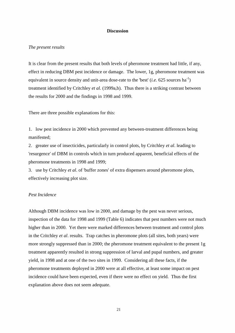
21

Discussion

The present results

It is clear from the present results that both levels of pheromone treatment had little, if any,

effect in reducing DBM pest incidence or damage. The lower, 1g, pheromone treatment was

equivalent in source density and unit-area dose-rate to the 'best' (i.e. 625 sources ha-1

)

treatment identified by Critchley et al. (1999a,b). Thus there is a striking contrast between

the results for 2000 and the findings in 1998 and 1999.

There are three possible explanations for this:

1. low pest incidence in 2000 which prevented any between-treatment differences being

manifested;

2. greater use of insecticides, particularly in control plots, by Critchley et al. leading to

'resurgence' of DBM in controls which in turn produced apparent, beneficial effects of the

pheromone treatments in 1998 and 1999;

3. use by Critchley et al. of 'buffer zones' of extra dispensers around pheromone plots,

effectively increasing plot size.

Pest Incidence

Although DBM incidence was low in 2000, and damage by the pest was never serious,

inspection of the data for 1998 and 1999 (Table 6) indicates that pest numbers were not much

higher than in 2000. Yet there were marked differences between treatment and control plots

in the Critchley et al. results. Trap catches in pheromone plots (all sites, both years) were

more strongly suppressed than in 2000; the pheromone treatment equivalent to the present 1g

treatment apparently resulted in strong suppression of larval and pupal numbers, and greater

yield, in 1998 and at one of the two sites in 1999. Considering all these facts, if the

pheromone treatments deployed in 2000 were at all effective, at least some impact on pest

incidence could have been expected, even if there were no effect on yield. Thus the first

explanation above does not seem adequate.

22

Table 6. Summary comparison of results between data of Critchley et al. (1999a,b) and

2000 trials in Kenya.

1998 & 1999 2000

Mean weekly trap catches

(control plots)

Mostly 2 - 10, peaks 25 - 45 Mostly 5 - 10, peaks 20 - 25

Larval + pupal incidence

per plant

Mostly 0.5 - 2.0, end-of-season

peaks 4.5 - 35.0 (control plots)

Always < 1.0, except end-of-

season peak at Kabete of 6.0

(treatments and controls)

Yield Yield in 'best' density

pheromone plot 2 that in

control; no effect at lower

pheromone densities

No consistent differences in %

yield loss between control and

pheromone plots

Resurgence Effects

There is good evidence that 'resurgence' effects could explain the results obtained by

Critchley et al. (1999a,b). In those trials the control plots were intended to reflect farmer

practice and as such, consistently more insecticides were applied than in the respective

pheromone treated plots (Table 7).

In three separate comparative pesticide trials carried out in Kenya under the Vegetable IPM

project (A0848), DBM larval numbers were consistently higher in plots treated with

Pirimicarb and the pyrethroid -Cyhalothrin, than in unsprayed plots. Populations of syrphid

fly larvae (predators of DBM) were also reduced in the sprayed plots. The same effects were

noted in respect of -Cyhalothrin in three 'hand-picking' trials, and in these cases there was

evidence that spider populations were also reduced. It is possible that similar effects may

have occured with other pesticides used in the 1998 and 1999 pheromone trials, particularly

the pyrethroid -Cypermethrin. It can be further noted that populations of syrphid fly larvae

were lower in control plots at two of the three sites in the 1998 trials (no data on beneficial

arthropods were recorded for 1999), and that pyrethroids were only sprayed in control plots.

Thus, there is a very strong argument that the lower populations of DBM observed in the

pheromone plots of 1998 and 1999 were due to a lack of resurgence effects there, compared

to the more heavily insecticide-sprayed control plots. Such could not have been the case in

2000.

23

Table 7. Summary comparison of insecticide applications in 1998, 1999 and 2000 trials in

Kenya.

1998 1999 2000

Sprays in

pheromone plots

1 - 3 0 - 2 1 - 2

Sprays in controls 2 - 5 4 - 9 1 - 2

Insecticides used Fenitrothion,

Pirimicarb,

-Cyhalothrin*

Including:

Fenitrothion,

Pirimicarb,

Dimethoate,

-Cypermethrin*

Chlorpyrifos

Pymetrozine,

Pirimicarb

* Not used in the respective pheromone plots

Use of 'Buffer Zones'

In their 1998 trials Critchley and his co-workers employed 4 - 8 m wide 'buffer zones' around

the edges of the pheromone plots. It is conceivable that these contributed to the apparent

beneficial effects of pheromone treatment observed, as they would have nearly doubled the

effective plot size. In support of this it may be noted that results in 1998 were somewhat

better than in 1999, when buffer zones were not used.

Plot size is usually considered an important factor governing the effectiveness of mating-

disruption treatments - and most successful control has been in plots of at least 1 ha. Having

a large, contiguous area of treated crop is advantageous in two ways. Firstly, the diluting

effect of wind upon aerial concentrations of the pheromone within the plot is minimised, at

least away from the field edges. Secondly, if immigration of previously mated female insects

occurs, it is less likely that all of the plot will be affected if it is sufficiently large.

Other mating-disruption studies with DBM

As noted in the Introduction, trials conducted by Ohbayashi et al. (1992), Nemoto et al.

(1992), Ohno et al. (1992), McLaughlin et al. (1994) and Mitchell et al. (1997) have all

produced good control of DBM in pheromone plots compared to their respective controls. All

of these results were obtained using commercial „rope‟ formulations consisting of a tube

filled with the pheromone and stiffened with wire, and nearly all utilised only the two major

pheromone components, Z11-16:Ald and Z11-16:Ac.

24

All of the above-mentioned trials used at least 250 g ha-1

of pheromone, with the exception of

that by Nemoto et al. (1992), which employed only 50 g ha-1

. Interestingly, it was in this

case that the results were least convincing. Specifically, trap captures of male DBM in the

pheromone plots were less suppressed, relative to untreated controls, than in the other trials

and larval incidence was lower than the controls only on the last sampling date. This seems

to underline the importance of high application rates.

Ohbayashi et al. (1992) reported a series of nine trials, using unsprayed controls, carried out

in open fields over a range of locations, and plot sizes – mostly between 3 and 14 ha.

Application rates were 250 g ha-1

a.i. Trap catches in pheromone plots were typically reduced

by 90% compared to controls, levels of mating suppression ranged from 50 – 100%, while

larval reduction varied from 10 – 99%. Control was generally poorer in smaller fields, and in

fields exposed to winds. In one field of 0.8 ha control was good in the centre, but poor at the

edge. In a separate trial, mating suppression of almost 100% was achieved in 0.1 ha plots

that were enclosed under a greenhouse, so as to be airtight. In the same plots mating

suppression was poor when the plot was ventilated. Ohbayashi et al. (1992) concluded that

successful mating disruption was not possible in small plots and at sites exposed to wind.

These conclusions were somewhat contradicted by the findings of Ohno et al. (1992). They

found strong (~90%) trap-catch and mating suppression, and lower incidence of larvae in

open field plots of only 0.1 ha (one in an exposed location), also treated at a rate of

250 g ha-1

. Here again, controls were untreated.

McLaughlin et al. (1994) and Mitchell et al. (1997), working on commercial cabbage farms

in Florida, used pheromone plot sizes of 8.1 and 24.6 ha, and application rates of 250 and

406 g ha-1

, respectively. In these cases the control plots received many more applications of

insecticide than the pheromone plots. Thus the results - strong trap-catch suppression and

reduction of larval numbers below an economic threshold in pheromone plots, relative to

controls - might be ascribed to resurgence effects in the controls, as with the Critchley et al.

results. However, the strong suppression of mating of sentinel females in the pheromone

plots indicated a large mating disrupting effect, and argued against that conclusion. In the

pheromone plots, greater crop damage was noted at the edges than in the centre. This was

consistent with mating disruption working over most of the plots, but breaking down at the

edges.

25

With regard to plot size the findings by Schroeder et al. (2000), also in small (0.2 ha) plots of

cabbage, were interesting. A series of three trials compared pheromone applied at 275 g ha-1

with untreated controls and, unlike most other trials, treatments were replicated. Several field

cages were deployed within plots; at the start of the trials these were inoculated with different

densities of DBM pupae. Pheromone traps and 'sentinel' females were deployed within the

field cages to assess the ability of males to locate females. Irrespective of the initial DBM

density, no effect of the pheromone treatment was found on the proportion of mated sentinel

females, or on the numbers of F1 larvae and pupae found on cabbage plants. Significant trap-

catch suppression only occurred in two of the three trials. Although the use of the field cages

allowed the effect of the pheromone to be tested under several simulated population densities,

and allowed possible effects of immigration or emigration to be discounted, they may have

masked mating disruption effects. This could be because within the cages, males were never

far from sentinel females, and did not need to follow their pheromone plumes far upwind,

against a background of competing plumes from synthetic sources, as would otherwise be the

case in a mating disruption plot. Instead, matings could have occurred following chance

encounters. A similar effect could have occurred with respect to trap catches.

Limitations of the methods used in the 2000 trials

The design of the trial - with single replicates of each treatment and the control at separate

sites, meant that there was no useful statistical analysis that could be applied to the data. In

the present case this may not greatly matter, since visual inspection of the data is sufficient to

indicate that no treatment differences occurred (except perhaps in the case of the pheromone

trap catches). However, clearly it would be preferable to be able to analyse the data with

some form of parametric test. The problem can only be avoided if there are at least two

replicates of each treatment at each site.

The larval sampling method examined three groups of nine neighbouring plants per plot.

Given the large size of the plots, a better, more representative sampling method might look at

a larger number of groups, consisting of fewer plants.

Pheromone traps were monitored in order to provide a measure of the extent to which mating

of DBM was disrupted in the respective plots. This assumed that the ability of males to

orient towards both traps and females, is well correlated. In general this may not always be

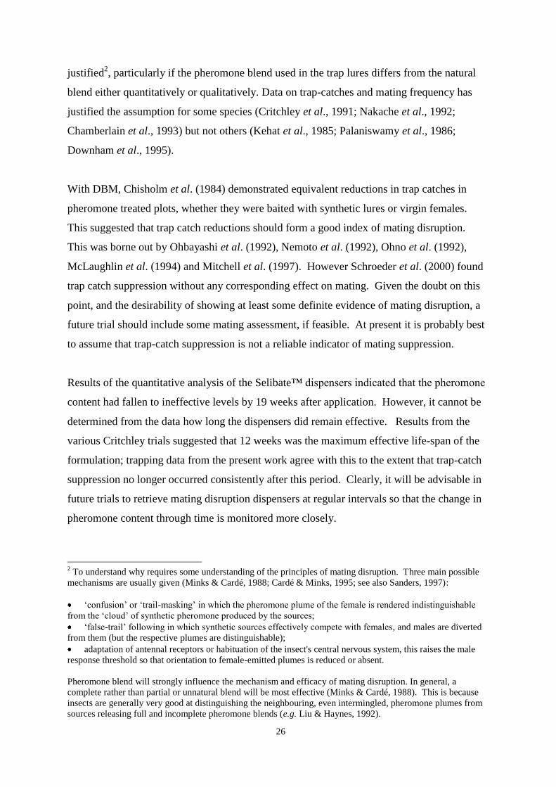
26

justified2, particularly if the pheromone blend used in the trap lures differs from the natural

blend either quantitatively or qualitatively. Data on trap-catches and mating frequency has

justified the assumption for some species (Critchley et al., 1991; Nakache et al., 1992;

Chamberlain et al., 1993) but not others (Kehat et al., 1985; Palaniswamy et al., 1986;

Downham et al., 1995).

With DBM, Chisholm et al. (1984) demonstrated equivalent reductions in trap catches in

pheromone treated plots, whether they were baited with synthetic lures or virgin females.

This suggested that trap catch reductions should form a good index of mating disruption.

This was borne out by Ohbayashi et al. (1992), Nemoto et al. (1992), Ohno et al. (1992),

McLaughlin et al. (1994) and Mitchell et al. (1997). However Schroeder et al. (2000) found

trap catch suppression without any corresponding effect on mating. Given the doubt on this

point, and the desirability of showing at least some definite evidence of mating disruption, a

future trial should include some mating assessment, if feasible. At present it is probably best

to assume that trap-catch suppression is not a reliable indicator of mating suppression.

Results of the quantitative analysis of the Selibate™ dispensers indicated that the pheromone

content had fallen to ineffective levels by 19 weeks after application. However, it cannot be

determined from the data how long the dispensers did remain effective. Results from the

various Critchley trials suggested that 12 weeks was the maximum effective life-span of the

formulation; trapping data from the present work agree with this to the extent that trap-catch

suppression no longer occurred consistently after this period. Clearly, it will be advisable in

future trials to retrieve mating disruption dispensers at regular intervals so that the change in

pheromone content through time is monitored more closely.

2 To understand why requires some understanding of the principles of mating disruption. Three main possible

mechanisms are usually given (Minks & Cardé, 1988; Cardé & Minks, 1995; see also Sanders, 1997):

„confusion‟ or „trail-masking‟ in which the pheromone plume of the female is rendered indistinguishable

from the „cloud‟ of synthetic pheromone produced by the sources;

„false-trail‟ following in which synthetic sources effectively compete with females, and males are diverted

from them (but the respective plumes are distinguishable);

adaptation of antennal receptors or habituation of the insect's central nervous system, this raises the male

response threshold so that orientation to female-emitted plumes is reduced or absent.

Pheromone blend will strongly influence the mechanism and efficacy of mating disruption. In general, a

complete rather than partial or unnatural blend will be most effective (Minks & Cardé, 1988). This is because

insects are generally very good at distinguishing the neighbouring, even intermingled, pheromone plumes from

sources releasing full and incomplete pheromone blends (e.g. Liu & Haynes, 1992).

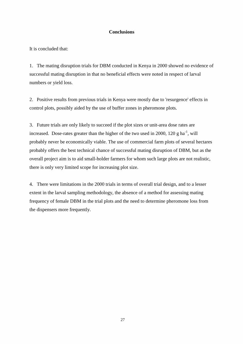
27

Conclusions

It is concluded that:

1. The mating disruption trials for DBM conducted in Kenya in 2000 showed no evidence of

successful mating disruption in that no beneficial effects were noted in respect of larval

numbers or yield loss.

2. Positive results from previous trials in Kenya were mostly due to 'resurgence' effects in

control plots, possibly aided by the use of buffer zones in pheromone plots.

3. Future trials are only likely to succeed if the plot sizes or unit-area dose rates are

increased. Dose-rates greater than the higher of the two used in 2000, 120 g ha-1

, will

probably never be economically viable. The use of commercial farm plots of several hectares

probably offers the best technical chance of successful mating disruption of DBM, but as the

overall project aim is to aid small-holder farmers for whom such large plots are not realistic,

there is only very limited scope for increasing plot size.

4. There were limitations in the 2000 trials in terms of overall trial design, and to a lesser

extent in the larval sampling methodology, the absence of a method for assessing mating

frequency of female DBM in the trial plots and the need to determine pheromone loss from

the dispensers more frequently.

28

Specific Recommendations for a Further Trial

1. Future trials should use 0.1 ha plots as before, but should compare untreated controls with

mating-disruption plots where the array of dispensers covers the kale plot itself and a

substantial 'buffer zone' outside so that a total area of 0.2 ha is covered.

2. A single dose-rate of 120 g ha-1

should be tested and the density of dispensers within the

treatment plots should be doubled to 1250 ha-1

.

3. The trial design should consist of 3 controls and 3 treated plots, if possible at a single site

(so that analysis of variance can be applied to any results). As before, trial plots (including

buffer zones) should be separated by a minimum of 50 m.

4. The larval sampling method should examine seven groups of four neighbouring plants per

plot.

5. Some assessment of mating by female DBM should be attempted on at least two

occasions during the trial.

6. Samples of Selibate dispensers should be taken from the fields at 2 week intervals for

subsequent quantitative analysis.

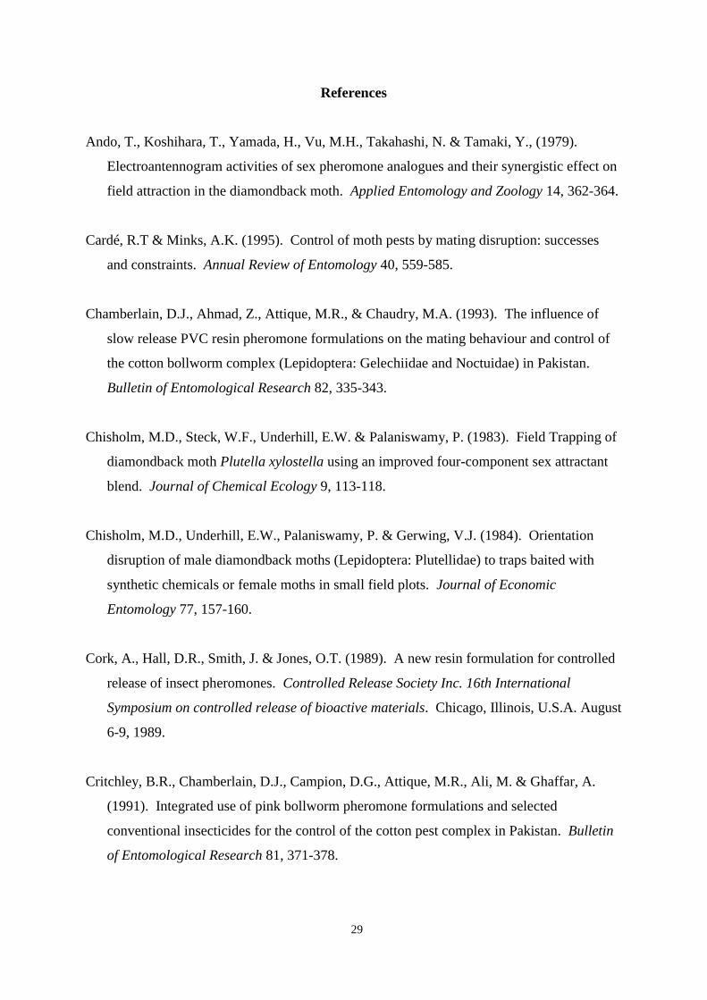
29

References

Ando, T., Koshihara, T., Yamada, H., Vu, M.H., Takahashi, N. & Tamaki, Y., (1979).

Electroantennogram activities of sex pheromone analogues and their synergistic effect on

field attraction in the diamondback moth. Applied Entomology and Zoology 14, 362-364.

Cardé, R.T & Minks, A.K. (1995). Control of moth pests by mating disruption: successes

and constraints. Annual Review of Entomology 40, 559-585.

Chamberlain, D.J., Ahmad, Z., Attique, M.R., & Chaudry, M.A. (1993). The influence of

slow release PVC resin pheromone formulations on the mating behaviour and control of

the cotton bollworm complex (Lepidoptera: Gelechiidae and Noctuidae) in Pakistan.

Bulletin of Entomological Research 82, 335-343.

Chisholm, M.D., Steck, W.F., Underhill, E.W. & Palaniswamy, P. (1983). Field Trapping of

diamondback moth Plutella xylostella using an improved four-component sex attractant

blend. Journal of Chemical Ecology 9, 113-118.

Chisholm, M.D., Underhill, E.W., Palaniswamy, P. & Gerwing, V.J. (1984). Orientation

disruption of male diamondback moths (Lepidoptera: Plutellidae) to traps baited with

synthetic chemicals or female moths in small field plots. Journal of Economic

Entomology 77, 157-160.

Cork, A., Hall, D.R., Smith, J. & Jones, O.T. (1989). A new resin formulation for controlled

release of insect pheromones. Controlled Release Society Inc. 16th International

Symposium on controlled release of bioactive materials. Chicago, Illinois, U.S.A. August

6-9, 1989.

Critchley, B.R., Chamberlain, D.J., Campion, D.G., Attique, M.R., Ali, M. & Ghaffar, A.

(1991). Integrated use of pink bollworm pheromone formulations and selected

conventional insecticides for the control of the cotton pest complex in Pakistan. Bulletin

of Entomological Research 81, 371-378.

30

Critchley, B.R., Farman, D.I., Hall, D.R., Ong'aro, J.M., Kibata, G.N., Olubayo, F., Nbuvi,

J.N., Kaibui, M. & Kamau, C. (1998). Biorational control technologies for the integrated

pest management of diamondback moth, Plutella xylostella, on brassica crops in Kenya. I.

Use of sex pheromones: trap designs, pheromone blends and the optimum rate of

application of a novel slow release formulation for monitoring and communication

disruption. Unpublished report, Natural Resources Institute. 45 pp.

Critchley, B.R., Farman, D.I., Ong'aro, J.M., Kibata, G.N., Olubayo, F. & Kaibui, M.

(1999a). Biorational control technologies for the integrated pest management of

diamondback moth, Plutella xylostella, on brassica crops. II. Mating disruption trials

during the major rainy season, May to September 1998. Unpublished report, Natural

Resources Institute. 36 pp.


(1999b). Biorational control technologies for the integrated pest management of

diamondback moth, Plutella xylostella, on brassica crops. III. Mating disruption trials

during the major dry season, February to April 1999. Unpublished report, Natural


Downham, M.C.A., McVeigh, L.J. & Moawad, G.M. (1995). Field investigation of an

attracticide control technique using the sex pheromone of the Egyptian cotton leafworm,

Spodoptera littoralis (Lepidoptera: Noctuidae). Bulletin of Entomological Research 85,

463-472.

Kawasaki, K. (1984). Effects of ratio and amount of the two sex pheromonal components of

the diamondback moth on male behavioural response. Applied Entomology and Zoology

19, 436-442.

Kehat, M., Gothlif, S., Dunkelblum, E., Bar Shavit, N. & Gordon, D. (1985). Night

observations on the cotton leafworm, Spodoptera littoralis: reliability of pheromone traps

for population assessment and efficacy of widely separated pheromone dispensers for

mating disruption. Phytoparasitica 13, 215-220.

31

Koshihara, T. & Yamada, H. (1980). Attractant activity of the female sex pheromone of the

diamondback moth, Plutella xylostella (L.) and analogue. Japanese Journal of Applied

Entomology and Zoology 24, 6-12.

Koshihara, T., Yamada, H., Tamaki, Y. & Ando, T. (1978). Field attractiveness of the

synthetic sex pheromone of the diamondback moth, Plutella xylostella (L.) and analogue.

Applied Entomology and Zoology 13, 138-141.

Liu, Y.-B. & Haynes, K.F. (1992). Filamentous nature of pheromone plumes protects

integrity of signal from background chemical noise in cabbage looper moth Trichoplusia

ni. Journal of Chemical Ecology 18, 299-307.

McLaughlin, J.R., Mitchell, E.R. & Kirsch, P. (1994). Mating disruption of diamondback

moth (Lepidoptera: Plutellidae) in cabbage: reduction of mating and suppression of larval

populations. Journal of Economic Entomology 87, 1198-1204.

Minks, A. & Cardé, R.T. (1988). Disruption of pheromone communication in moths: is the

natural blend really most efficacious? Entomologia Experimentalis et Applicata 49, 25-

36.

Mitchell, E.R., Hu, G.Y., Okine, J. & McLaughlin, J.R.,. (1997). Mating disruption of

diamondback moth (Lepidoptera: Plutellidae) and cabbage looper (Lepidoptera:

Noctuidae) in cabbage using a blend of pheromones emitted from the same dispenser.

Journal of Entomological Science 32, 120-137.

Nakache, J., Dunkelblum, E., Kehat, M., Anshelevich, L. & Harel, M. (1992). Mating

disruption of the spiny bollworm, Earias insulana (Lepidoptera: Noctuidae), with Shin-

Etsu twist-tie ropes in Israel. Bulletin of Entomological Research 82, 369-373.

Nemoto, H., Yano, E. & Kiritani, K. (1992). Pheromonal control of diamondback moth in the

management of crucifer pests. In: Talekar, N.S. (ed.). Diamondback moth and other

crucifer pests. Proceedings of the Second International Workshop, Tainin, Taiwan, 10-14

December 1990. Asian Vegetable Research and Development Center, pp. 91-97.

32

Ohbayashi, N., Shimizu, K. & Nagata, K. (1992). Control of diamondback moth using

synthetic sex pheromones. In: Talekar, N.S. (ed.). Diamondback moth and other crucifer

pests. Proceedings of the Second International Workshop, Tainin, Taiwan, 10-14

December 1990. Asian Vegetable Research and Development Center, pp. 99-104.

Ohno, T., Asayama., T. & Ichikawa, K. (1992). Evaluation of communication disruption

method using synthetic sex pheromone to suppress diamondback moth infestations. In:

Talekar, N.S. (ed.). Diamondback moth and other crucifer pests. Proceedings of the

Second International Workshop, Tainin, Taiwan, 10-14 December 1990. Asian

Vegetable Research and Development Center, pp. 109-114.

Palaniswamy, P., Underhill, E.W., Gillot, C. & Wong, J.W. (1986). Synthetic sex pheromone

components disrupt orientation, but not mating, in the fall cankerworm, Alsophila

pometaria (Lepidoptera: Geometridae). Environmental Entomology 15, 943-950.

Sanders, C.J. (1997). Mechanisms of mating disruption in moths. In: Cardé, R.T. & Minks,

A.K. (eds.). Insect Pheromone Research: New Directions. Chapman & Hall, New York.

Schroeder, P.C., Shelton, A.M., Ferguson, C.S., Hoffmann, M.P. & Petzoldt, C.H. (2000).

Application of synthetic sex pheromone for management of diamondback moth, Plutella

xylostella, in cabbage. Entomologia Experimentalis et Applicata 94, 243-248.

Talekar, N.S. & Shelton, A.M. (1993). Biology, ecology and management of the

diamondback moth. Annual Review of Entomology 38, 275-301.

Tamaki, Y., Kawasaki, K., Yamada, H., Koshihara, T., Osaki, N., Ando, T., Yoshida, S. &

Kakinohana, H. (1977). (Z)-11-hexadecenal and (Z)-11-hexadecenyl acetate: sex

pheromone components of the diamondback moth (Lepidoptera: Plutellidae). Applied

Entomology and Zoology 12, 208-210.

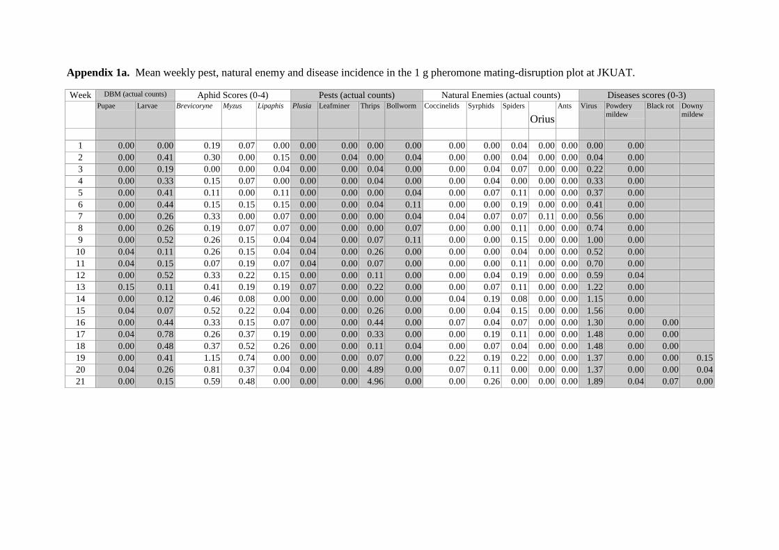
Appendix 1a. Mean weekly pest, natural enemy and disease incidence in the 1 g pheromone mating-disruption plot at JKUAT.

Week DBM (actual counts) Aphid Scores (0-4) Pests (actual counts) Natural Enemies (actual counts) Diseases scores (0-3)

Pupae Larvae Brevicoryne Myzus Lipaphis Plusia Leafminer Thrips Bollworm Coccinelids Syrphids Spiders

Orius

Ants Virus Powdery

mildew

Black rot Downy

mildew

1 0.00 0.00 0.19 0.07 0.00 0.00 0.00 0.00 0.00 0.00 0.00 0.04 0.00 0.00 0.00 0.00

2 0.00 0.41 0.30 0.00 0.15 0.00 0.04 0.00 0.04 0.00 0.00 0.04 0.00 0.00 0.04 0.00

3 0.00 0.19 0.00 0.00 0.04 0.00 0.00 0.04 0.00 0.00 0.04 0.07 0.00 0.00 0.22 0.00

4 0.00 0.33 0.15 0.07 0.00 0.00 0.00 0.04 0.00 0.00 0.04 0.00 0.00 0.00 0.33 0.00

5 0.00 0.41 0.11 0.00 0.11 0.00 0.00 0.00 0.04 0.00 0.07 0.11 0.00 0.00 0.37 0.00

6 0.00 0.44 0.15 0.15 0.15 0.00 0.00 0.04 0.11 0.00 0.00 0.19 0.00 0.00 0.41 0.00

7 0.00 0.26 0.33 0.00 0.07 0.00 0.00 0.00 0.04 0.04 0.07 0.07 0.11 0.00 0.56 0.00

8 0.00 0.26 0.19 0.07 0.07 0.00 0.00 0.00 0.07 0.00 0.00 0.11 0.00 0.00 0.74 0.00

9 0.00 0.52 0.26 0.15 0.04 0.04 0.00 0.07 0.11 0.00 0.00 0.15 0.00 0.00 1.00 0.00

10 0.04 0.11 0.26 0.15 0.04 0.04 0.00 0.26 0.00 0.00 0.00 0.04 0.00 0.00 0.52 0.00

11 0.04 0.15 0.07 0.19 0.07 0.04 0.00 0.07 0.00 0.00 0.00 0.11 0.00 0.00 0.70 0.00

12 0.00 0.52 0.33 0.22 0.15 0.00 0.00 0.11 0.00 0.00 0.04 0.19 0.00 0.00 0.59 0.04

13 0.15 0.11 0.41 0.19 0.19 0.07 0.00 0.22 0.00 0.00 0.07 0.11 0.00 0.00 1.22 0.00

14 0.00 0.12 0.46 0.08 0.00 0.00 0.00 0.00 0.00 0.04 0.19 0.08 0.00 0.00 1.15 0.00

15 0.04 0.07 0.52 0.22 0.04 0.00 0.00 0.26 0.00 0.00 0.04 0.15 0.00 0.00 1.56 0.00

16 0.00 0.44 0.33 0.15 0.07 0.00 0.00 0.44 0.00 0.07 0.04 0.07 0.00 0.00 1.30 0.00 0.00

17 0.04 0.78 0.26 0.37 0.19 0.00 0.00 0.33 0.00 0.00 0.19 0.11 0.00 0.00 1.48 0.00 0.00

18 0.00 0.48 0.37 0.52 0.26 0.00 0.00 0.11 0.04 0.00 0.07 0.04 0.00 0.00 1.48 0.00 0.00

19 0.00 0.41 1.15 0.74 0.00 0.00 0.00 0.07 0.00 0.22 0.19 0.22 0.00 0.00 1.37 0.00 0.00 0.15

20 0.04 0.26 0.81 0.37 0.04 0.00 0.00 4.89 0.00 0.07 0.11 0.00 0.00 0.00 1.37 0.00 0.00 0.04

21 0.00 0.15 0.59 0.48 0.00 0.00 0.00 4.96 0.00 0.00 0.26 0.00 0.00 0.00 1.89 0.04 0.07 0.00

ii

Appendix 1b. Mean weekly pest, natural enemy and disease incidence in the 2 g pheromone mating-disruption plot at JKUAT.



Oriu

s

Ants Virus Powdery

mildew

Black rot Downy

mildew

1 0.00 0.04 0.04 0.00 0.04 0.00 0.00 0.00 0.00 0.00 0.00 0.00 0.00 0.00 0.00 0.00

2 0.00 0.00 0.19 0.00 0.11 0.00 0.00 0.00 0.00 0.00 0.00 0.04 0.00 0.00 0.30 0.00

3 0.04 0.19 0.19 0.04 0.07 0.00 0.00 0.00 0.07 0.00 0.04 0.04 0.00 0.00 0.74 0.00

4 0.00 1.00 0.26 0.07 0.00 0.04 0.00 0.00 0.04 0.04 0.19 0.15 0.00 0.00 0.89 0.00

5 0.00 0.41 0.11 0.04 0.19 0.07 0.00 0.00 0.15 0.00 0.30 0.15 0.00 0.00 0.85 0.00

6 0.00 0.41 0.22 0.04 0.04 0.00 0.00 0.00 0.07 0.04 0.00 0.07 0.00 0.00 1.00 0.00

7 0.04 0.48 0.30 0.07 0.04 0.00 0.00 0.00 0.11 0.00 0.00 0.07 0.00 0.00 0.89 0.00

8 0.04 0.44 0.19 0.00 0.07 0.07 0.00 0.00 0.00 0.00 0.00 0.33 0.00 0.00 0.56 0.00

9 0.00 0.74 0.33 0.07 0.11 0.00 0.00 0.11 0.00 0.00 0.00 0.26 0.00 0.00 1.30 0.00

10 0.00 0.41 0.07 0.00 0.00 0.00 0.00 0.04 0.00 0.00 0.00 0.26 0.00 0.00 0.74 0.00

11 0.00 0.22 0.11 0.11 0.07 0.00 0.00 0.07 0.00 0.04 0.00 0.19 0.00 0.00 1.00 0.00

12 0.11 0.41 0.19 0.00 0.15 0.00 0.00 0.07 0.04 0.00 0.00 0.11 0.00 0.00 0.89 0.00

13 0.04 0.63 0.11 0.15 0.44 0.00 0.00 0.48 0.00 0.19 0.11 0.00 0.00 0.00 1.11 0.00

14 0.07 0.37 0.07 0.15 0.15 0.00 0.00 0.00 0.04 0.00 0.11 0.07 0.00 0.00 1.07 0.00

15 0.04 0.33 0.11 0.19 0.07 0.00 0.00 0.67 0.00 0.11 0.07 0.15 0.00 0.00 1.63 0.00

16 0.00 0.56 0.07 0.07 0.04 0.00 0.00 1.00 0.04 0.04 0.07 0.07 0.00 0.00 1.26 0.00 0.04

17 0.07 0.67 0.07 0.22 0.11 0.00 0.00 0.26 0.00 0.07 0.04 0.07 0.00 0.00 1.78 0.00 0.11

18 0.00 1.26 0.15 0.33 0.19 0.00 0.00 1.30 0.00 0.07 0.07 0.11 0.00 0.00 1.63 0.00 0.00

19 0.04 0.74 0.44 0.41 0.11 0.00 0.00 0.67 0.00 0.00 0.11 0.11 0.00 0.00 1.30 0.00 0.11 0.22

20 0.07 0.67 0.59 0.33 0.11 0.00 0.00 6.44 0.00 0.19 0.04 0.11 0.00 0.00 1.41 0.00 0.04 0.26

21 0.04 0.81 0.41 0.22 0.07 0.00 0.00 8.19 0.00 0.15 0.22 0.07 0.00 0.00 1.48 0.04 0.11 0.00

iii

Appendix 1c. Mean weekly pest, natural enemy and disease incidence in the control plot at JKUAT.



Oriu

s

Ants Virus Powdery

mildew

Black rot Downy

mildew

1 0.07 0.00 0.15 0.00 0.00 0.00 0.00 0.04 0.00 0.00 0.00 0.00 0.00 0.07 0.00 0.00

2 0.00 0.22 0.04 0.07 0.04 0.00 0.00 0.00 0.04 0.00 0.00 0.04 0.00 0.00 0.04 0.00

3 0.00 0.15 0.07 0.00 0.04 0.04 0.00 0.00 0.00 0.04 0.07 0.07 0.00 0.00 0.37 0.00

4 0.00 0.81 0.15 0.07 0.19 0.00 0.00 0.00 0.00 0.00 0.00 0.07 0.00 0.00 0.44 0.00

5 0.00 0.67 0.26 0.07 0.26 0.04 0.00 0.00 0.04 0.00 0.19 0.15 0.00 0.00 0.67 0.00

6 0.00 0.33 0.22 0.00 0.04 0.00 0.00 0.00 0.11 0.04 0.00 0.30 0.00 0.00 0.48 0.00

7 0.00 0.48 0.15 0.07 0.04 0.04 0.00 0.00 0.07 0.00 0.00 0.15 0.00 0.00 0.70 0.00

8 0.00 0.19 0.22 0.15 0.11 0.00 0.00 0.00 0.04 0.00 0.00 0.00 0.00 0.00 0.67 0.00

9 0.00 0.56 0.33 0.00 0.07 0.04 0.00 0.04 0.00 0.00 0.00 0.19 0.00 0.00 1.19 0.00

10 0.00 0.15 0.11 0.00 0.04 0.00 0.00 0.19 0.07 0.00 0.00 0.22 0.00 0.00 0.63 0.00

11 0.00 0.26 0.04 0.07 0.22 0.00 0.00 0.11 0.00 0.04 0.00 0.11 0.00 0.00 1.11 0.00

12 0.04 0.63 0.07 0.04 0.11 0.00 0.00 0.67 0.00 0.00 0.00 0.00 0.00 0.00 0.70 0.00

13 0.04 0.11 0.11 0.07 0.30 0.07 0.00 0.56 0.00 0.00 0.00 0.11 0.00 0.00 1.19 0.00

14 0.00 0.26 0.19 0.04 0.11 0.00 0.00 0.15 0.07 0.07 0.00 0.00 0.00 0.00 1.30 0.00

15 0.04 0.11 0.11 0.22 0.07 0.04 0.00 0.19 0.00 0.00 0.04 0.15 0.00 0.00 1.41 0.00

16 0.00 0.41 0.33 0.44 0.00 0.00 0.00 0.07 0.00 0.11 0.00 0.04 0.00 0.04 1.33 0.00 0.00

17 0.04 0.44 0.41 0.33 0.15 0.00 0.00 0.22 0.00 0.04 0.07 0.07 0.00 0.00 1.81 0.00 0.00

18 0.11 1.04 0.59 0.48 0.15 0.00 0.00 1.33 0.00 0.00 0.04 0.00 0.00 0.00 1.41 0.00 0.00

19 0.11 0.11 0.67 0.56 0.15 0.04 0.00 1.00 0.00 0.00 0.07 0.19 0.00 0.00 1.37 0.00 0.00 0.22

20 0.15 0.63 0.59 0.33 0.11 0.00 0.00 6.89 0.00 0.07 0.15 0.07 0.00 0.00 1.22 0.00 0.00 0.07

21 0.19 0.89 0.63 0.37 0.07 0.00 0.00 6.81 0.00 0.22 0.07 0.15 0.00 0.00 1.70 0.00 0.04 0.04

iv

Appendix 2a. Mean weekly pest, natural enemy and disease incidence in the 1 g pheromone mating-disruption plot at Ongata Rongai.



Oriu

s

Ants Virus Powdery

mildew

Black rot Downy

mildew

1 0.00 0.00 0.07 0.15 0.19 0.00 0.07 0.04 0.00 0.00 0.00 0.07 0.00 0.00 0.11 0.00

2 0.00 0.33 0.15 0.04 0.15 0.00 0.07 0.04 0.00 0.04 0.00 0.26 0.00 0.04 0.22 0.00

3 0.00 0.00 0.15 0.04 0.07 0.00 0.00 0.00 0.00 0.04 0.00 0.00 0.00 0.00 0.11 0.07

4 0.07 0.07 0.33 0.30 0.04 0.00 0.00 0.04 0.00 0.00 0.00 0.00 0.00 0.00 0.44 0.00

5 0.00 0.04 0.26 0.19 0.22 0.00 0.00 0.00 0.00 0.00 0.00 0.04 0.00 0.00 0.70 0.04

6 0.00 0.00 0.33 0.04 0.15 0.00 0.00 0.00 0.00 0.00 0.00 0.00 0.00 0.00 1.04 0.11

7 0.00 0.00 0.26 0.07 0.52 0.00 0.00 0.04 0.00 0.00 0.07 0.22 0.00 0.00 0.78 0.22

8 0.00 0.11 0.22 0.00 0.00 0.00 0.04 0.00 0.04 0.00 0.04 0.00 0.00 0.00 0.81 0.04

9 0.00 0.04 0.07 0.00 0.04 0.00 0.00 0.00 0.00 0.00 0.00 0.19 0.00 0.00 1.04 0.04

10 0.00 0.00 0.22 0.00 0.00 0.00 0.00 0.00 0.00 0.00 0.00 0.00 0.00 0.00 1.22 0.00

11 0.00 0.04 0.07 0.00 0.00 0.00 0.00 0.07 0.00 0.00 0.00 0.15 0.00 0.00 0.93 0.22

12 0.00 0.33 0.00 0.00 0.00 0.00 0.00 0.00 0.00 0.00 0.00 0.00 0.00 0.00 0.96 0.04

13 0.04 0.41 0.00 0.00 0.00 0.00 0.00 0.19 0.00 0.00 0.00 0.07 0.00 0.00 1.59 0.07

14 0.04 1.04 0.78 0.00 0.07 0.00 0.00 0.41 0.00 0.00 0.22 0.15 0.00 0.00 1.19 0.11

15 0.04 0.37 0.11 0.00 0.00 0.00 0.00 0.00 0.00 0.04 0.00 0.00 0.00 0.00 1.00 0.07 0.00 0.07

16 0.04 0.56 0.19 0.07 0.00 0.00 0.00 0.11 0.00 0.00 0.00 0.11 0.00 0.00 1.04 0.30 0.04 0.37

17 0.00 0.22 0.15 0.00 0.00 0.00 0.00 1.19 0.00 0.00 0.04 0.00 0.00 0.00 1.07 0.00 0.00 0.00

18 0.00 0.26 0.67 0.19 0.00 0.00 0.00 0.52 0.00 0.04 0.00 0.15 0.00 0.00 1.00 0.11 0.04 0.19

19 0.00 0.44 0.44 0.00 0.00 0.00 0.00 0.22 0.00 0.00 0.00 0.00 0.00 0.00 1.41 0.11 0.00 0.00

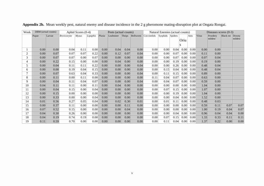
v

Appendix 2b. Mean weekly pest, natural enemy and disease incidence in the 2 g pheromone mating-disruption plot at Ongata Rongai. Week DBM (actual counts) Aphid Scores (0-4) Pests (actual counts) Natural Enemies (actual counts) Diseases scores (0-3)


Oriu

s

Ants Virus Powdery

mildew

Black rot Downy

mildew

1 0.00 0.00 0.04 0.11 0.00 0.00 0.04 0.04 0.00 0.00 0.00 0.04 0.00 0.00 0.00 0.00

2 0.00 0.07 0.07 0.07 0.22 0.00 0.12 0.07 0.04 0.00 0.00 0.07 0.00 0.00 0.11 0.00

3 0.00 0.07 0.07 0.00 0.07 0.00 0.00 0.00 0.00 0.00 0.00 0.07 0.00 0.00 0.07 0.04

4 0.00 0.22 0.15 0.00 0.00 0.00 0.04 0.00 0.00 0.00 0.00 0.19 0.00 0.00 0.19 0.00

5 0.00 0.04 0.11 0.11 0.22 0.00 0.00 0.00 0.04 0.00 0.00 0.26 0.00 0.00 0.48 0.04

6 0.00 0.00 0.19 0.04 0.15 0.00 0.00 0.00 0.00 0.00 0.15 0.04 0.00 0.00 0.48 0.04

7 0.00 0.07 0.63 0.04 0.33 0.00 0.00 0.00 0.04 0.00 0.11 0.15 0.00 0.00 0.89 0.00

8 0.00 0.11 0.00 0.11 0.00 0.00 0.00 0.00 0.00 0.11 0.04 0.07 0.00 0.00 0.63 0.00

9 0.00 0.04 0.11 0.04 0.07 0.00 0.00 0.00 0.04 0.00 0.04 0.07 0.00 0.00 0.59 0.00

10 0.04 0.11 0.11 0.00 0.11 0.00 0.04 0.00 0.00 0.00 0.00 0.00 0.00 0.00 1.04 0.00

11 0.00 0.04 0.15 0.00 0.04 0.00 0.00 0.00 0.00 0.00 0.07 0.15 0.00 0.00 1.07 0.00

12 0.00 0.15 0.00 0.00 0.00 0.00 0.00 0.00 0.00 0.00 0.00 0.19 0.00 0.00 1.04 0.00

13 0.00 0.33 0.00 0.00 0.04 0.00 0.00 0.00 0.00 0.00 0.00 0.04 0.00 0.00 1.52 0.00

14 0.01 0.56 0.27 0.05 0.04 0.00 0.02 0.30 0.01 0.00 0.01 0.11 0.00 0.00 0.48 0.03

15 0.00 0.37 0.11 0.00 0.00 0.00 0.00 0.11 0.00 0.00 0.00 0.00 0.00 0.00 0.59 0.11 0.07 0.07

16 0.07 0.52 0.15 0.00 0.00 0.00 0.00 0.04 0.00 0.00 0.00 0.00 0.00 0.00 1.00 0.19 0.04 0.07

17 0.04 0.30 0.26 0.00 0.00 0.00 0.00 0.00 0.00 0.00 0.00 0.04 0.00 0.00 0.96 0.04 0.04 0.00

18 0.04 0.19 0.74 0.19 0.00 0.00 0.00 0.00 0.00 0.00 0.07 0.15 0.00 0.00 1.33 0.33 0.11 0.11

19 0.11 0.59 0.70 0.00 0.00 0.00 0.00 0.00 0.00 0.00 0.11 0.04 0.00 0.00 1.37 0.22 0.00 0.00

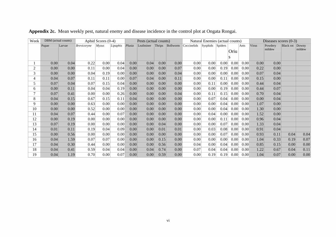
vi

Appendix 2c. Mean weekly pest, natural enemy and disease incidence in the control plot at Ongata Rongai.



Oriu

s

Ants Virus Powdery

mildew

Black rot Downy

mildew

1 0.00 0.04 0.22 0.00 0.04 0.00 0.04 0.00 0.00 0.00 0.00 0.00 0.00 0.00 0.00 0.00

2 0.00 0.00 0.11 0.00 0.04 0.00 0.00 0.00 0.07 0.00 0.00 0.19 0.00 0.00 0.22 0.00

3 0.00 0.00 0.04 0.19 0.00 0.00 0.00 0.00 0.04 0.00 0.00 0.00 0.00 0.00 0.07 0.04

4 0.04 0.07 0.11 0.11 0.00 0.07 0.04 0.00 0.11 0.00 0.00 0.11 0.00 0.00 0.15 0.00

5 0.07 0.04 0.07 0.15 0.04 0.00 0.00 0.00 0.00 0.00 0.11 0.00 0.00 0.00 0.44 0.04

6 0.00 0.11 0.04 0.04 0.19 0.00 0.00 0.00 0.00 0.00 0.00 0.19 0.00 0.00 0.44 0.07

7 0.07 0.41 0.00 0.00 0.26 0.00 0.00 0.00 0.04 0.00 0.11 0.15 0.00 0.00 0.70 0.04

8 0.04 0.15 0.67 0.15 0.11 0.04 0.00 0.00 0.00 0.00 0.07 0.04 0.00 0.00 0.00 0.04

9 0.00 0.00 0.63 0.00 0.00 0.00 0.00 0.00 0.00 0.00 0.00 0.04 0.00 0.00 1.07 0.00

10 0.00 0.00 0.52 0.00 0.00 0.00 0.00 0.00 0.00 0.00 0.00 0.04 0.00 0.00 1.30 0.00

11 0.04 0.07 0.44 0.00 0.07 0.00 0.00 0.00 0.00 0.00 0.04 0.00 0.00 0.00 1.52 0.00

12 0.00 0.19 0.00 0.00 0.00 0.00 0.00 0.00 0.00 0.00 0.00 0.11 0.00 0.00 0.96 0.04

13 0.07 0.19 0.00 0.00 0.00 0.00 0.00 0.04 0.00 0.00 0.00 0.07 0.00 0.00 1.33 0.04

14 0.01 0.11 0.19 0.04 0.09 0.00 0.00 0.01 0.01 0.00 0.03 0.08 0.00 0.00 0.91 0.04

15 0.00 0.56 0.00 0.00 0.00 0.00 0.00 0.00 0.00 0.00 0.00 0.07 0.00 0.00 0.93 0.11 0.04 0.04

16 0.04 1.59 0.07 0.07 0.00 0.00 0.00 0.15 0.00 0.00 0.00 0.00 0.00 0.00 1.04 0.33 0.19 0.07

17 0.04 0.30 0.44 0.00 0.00 0.00 0.00 0.56 0.00 0.04 0.00 0.04 0.00 0.00 0.85 0.15 0.00 0.00

18 0.04 0.41 0.59 0.04 0.04 0.00 0.04 0.74 0.00 0.07 0.04 0.04 0.00 0.00 1.22 0.67 0.04 0.11

19 0.04 1.19 0.70 0.00 0.07 0.00 0.00 0.59 0.00 0.00 0.19 0.19 0.00 0.00 1.04 0.07 0.00 0.00

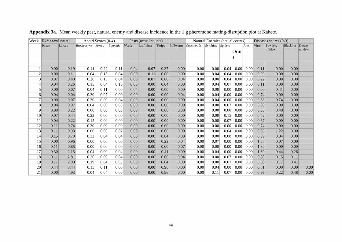
vii

Appendix 3a. Mean weekly pest, natural enemy and disease incidence in the 1 g pheromone mating-disruption plot at Kabete.



Oriu

s

Ants Virus Powdery

mildew

Black rot Downy

mildew

1 0.00 0.19 0.11 0.22 0.11 0.04 0.07 0.37 0.00 0.00 0.00 0.04 0.00 0.00 0.11 0.00 0.00

2 0.00 0.11 0.04 0.15 0.04 0.00 0.11 0.00 0.00 0.00 0.04 0.04 0.00 0.00 0.00 0.00 0.00

3 0.07 0.48 0.26 0.15 0.04 0.00 0.07 0.00 0.04 0.00 0.00 0.04 0.00 0.00 0.22 0.00 0.00

4 0.04 0.26 0.15 0.04 0.15 0.00 0.00 0.04 0.00 0.00 0.04 0.07 0.00 0.00 0.11 0.00 0.00

5 0.00 0.07 0.04 0.11 0.00 0.04 0.00 0.00 0.00 0.00 0.00 0.00 0.00 0.00 0.00 0.41 0.00

6 0.04 0.04 0.30 0.07 0.00 0.00 0.00 0.00 0.04 0.00 0.04 0.00 0.00 0.00 0.74 0.00 0.00

7 0.00 0.07 0.30 0.00 0.04 0.00 0.00 0.00 0.00 0.00 0.04 0.00 0.00 0.00 0.63 0.74 0.00

8 0.04 0.07 0.04 0.00 0.00 0.00 0.00 0.00 0.00 0.00 0.00 0.07 0.00 0.00 0.89 0.00 0.00

9 0.00 0.22 0.00 0.00 0.00 0.00 0.00 0.00 0.00 0.00 0.00 0.00 0.00 0.00 0.85 0.48 0.00

10 0.07 0.44 0.22 0.00 0.00 0.00 0.00 0.00 0.00 0.00 0.00 0.15 0.00 0.00 0.52 0.00 0.00

11 0.04 0.22 0.15 0.00 0.00 0.00 0.00 0.00 0.00 0.00 0.00 0.07 0.00 0.00 0.67 0.00 0.00

12 0.11 0.74 0.30 0.00 0.00 0.00 0.00 0.00 0.00 0.00 0.00 0.00 0.00 0.00 0.74 0.00 0.00

13 0.11 0.93 0.00 0.00 0.07 0.00 0.00 0.00 0.00 0.00 0.00 0.04 0.00 0.00 0.56 1.22 0.00

14 0.15 0.70 0.33 0.04 0.04 0.00 0.00 0.04 0.00 0.00 0.00 0.00 0.00 0.00 0.89 0.04 0.00

15 0.00 0.96 0.00 0.00 0.00 0.00 0.00 0.22 0.04 0.00 0.07 0.00 0.00 0.00 1.33 0.07 0.00

16 0.11 0.85 0.00 0.00 0.00 0.00 0.00 0.00 0.07 0.00 0.00 0.00 0.00 0.00 1.30 0.00 0.00

17 0.30 2.15 0.04 0.00 0.04 0.00 0.00 0.41 0.00 0.00 0.04 0.00 0.00 0.00 1.30 0.44 0.26

18 0.11 2.81 0.26 0.00 0.04 0.00 0.00 0.00 0.04 0.00 0.00 0.07 0.00 0.00 0.89 0.15 0.11

19 0.11 2.00 0.19 0.04 0.00 0.00 0.00 0.04 0.00 0.00 0.00 0.07 0.00 0.00 0.00 0.11 0.41

20 0.44 3.44 0.15 0.11 0.00 0.00 0.00 0.96 0.00 0.00 0.04 0.00 0.00 0.00 0.81 0.00 0.00 0.00

21 0.00 4.93 0.04 0.04 0.00 0.00 0.00 0.96 0.00 0.00 0.11 0.07 0.00 0.00 0.96 0.22 0.48 0.00

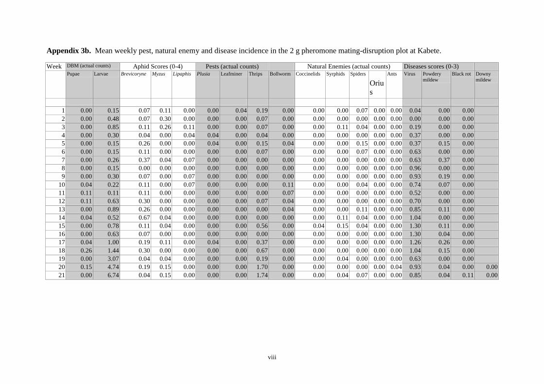
viii

Appendix 3b. Mean weekly pest, natural enemy and disease incidence in the 2 g pheromone mating-disruption plot at Kabete.



Oriu

s

Ants Virus Powdery

mildew

Black rot Downy

mildew

1 0.00 0.15 0.07 0.11 0.00 0.00 0.04 0.19 0.00 0.00 0.00 0.07 0.00 0.00 0.04 0.00 0.00

2 0.00 0.48 0.07 0.30 0.00 0.00 0.00 0.07 0.00 0.00 0.00 0.00 0.00 0.00 0.00 0.00 0.00

3 0.00 0.85 0.11 0.26 0.11 0.00 0.00 0.07 0.00 0.00 0.11 0.04 0.00 0.00 0.19 0.00 0.00

4 0.00 0.30 0.04 0.00 0.04 0.04 0.00 0.04 0.00 0.00 0.00 0.00 0.00 0.00 0.37 0.00 0.00

5 0.00 0.15 0.26 0.00 0.00 0.04 0.00 0.15 0.04 0.00 0.00 0.15 0.00 0.00 0.37 0.15 0.00

6 0.00 0.15 0.11 0.00 0.00 0.00 0.00 0.07 0.00 0.00 0.00 0.07 0.00 0.00 0.63 0.00 0.00

7 0.00 0.26 0.37 0.04 0.07 0.00 0.00 0.00 0.00 0.00 0.00 0.00 0.00 0.00 0.63 0.37 0.00

8 0.00 0.15 0.00 0.00 0.00 0.00 0.00 0.00 0.00 0.00 0.00 0.00 0.00 0.00 0.96 0.00 0.00

9 0.00 0.30 0.07 0.00 0.07 0.00 0.00 0.00 0.00 0.00 0.00 0.00 0.00 0.00 0.93 0.19 0.00

10 0.04 0.22 0.11 0.00 0.07 0.00 0.00 0.00 0.11 0.00 0.00 0.04 0.00 0.00 0.74 0.07 0.00

11 0.11 0.11 0.11 0.00 0.00 0.00 0.00 0.00 0.07 0.00 0.00 0.00 0.00 0.00 0.52 0.00 0.00

12 0.11 0.63 0.30 0.00 0.00 0.00 0.00 0.07 0.04 0.00 0.00 0.00 0.00 0.00 0.70 0.00 0.00

13 0.00 0.89 0.26 0.00 0.00 0.00 0.00 0.00 0.04 0.00 0.00 0.11 0.00 0.00 0.85 0.11 0.00

14 0.04 0.52 0.67 0.04 0.00 0.00 0.00 0.00 0.00 0.00 0.11 0.04 0.00 0.00 1.04 0.00 0.00

15 0.00 0.78 0.11 0.04 0.00 0.00 0.00 0.56 0.00 0.04 0.15 0.04 0.00 0.00 1.30 0.11 0.00

16 0.00 0.63 0.07 0.00 0.00 0.00 0.00 0.00 0.00 0.00 0.00 0.00 0.00 0.00 1.30 0.04 0.00

17 0.04 1.00 0.19 0.11 0.00 0.04 0.00 0.37 0.00 0.00 0.00 0.00 0.00 0.00 1.26 0.26 0.00

18 0.26 1.44 0.30 0.00 0.00 0.00 0.00 0.67 0.00 0.00 0.00 0.00 0.00 0.00 1.04 0.15 0.00

19 0.00 3.07 0.04 0.04 0.00 0.00 0.00 0.19 0.00 0.00 0.04 0.00 0.00 0.00 0.63 0.00 0.00

20 0.15 4.74 0.19 0.15 0.00 0.00 0.00 1.70 0.00 0.00 0.00 0.00 0.00 0.04 0.93 0.04 0.00 0.00

21 0.00 6.74 0.04 0.15 0.00 0.00 0.00 1.74 0.00 0.00 0.04 0.07 0.00 0.00 0.85 0.04 0.11 0.00

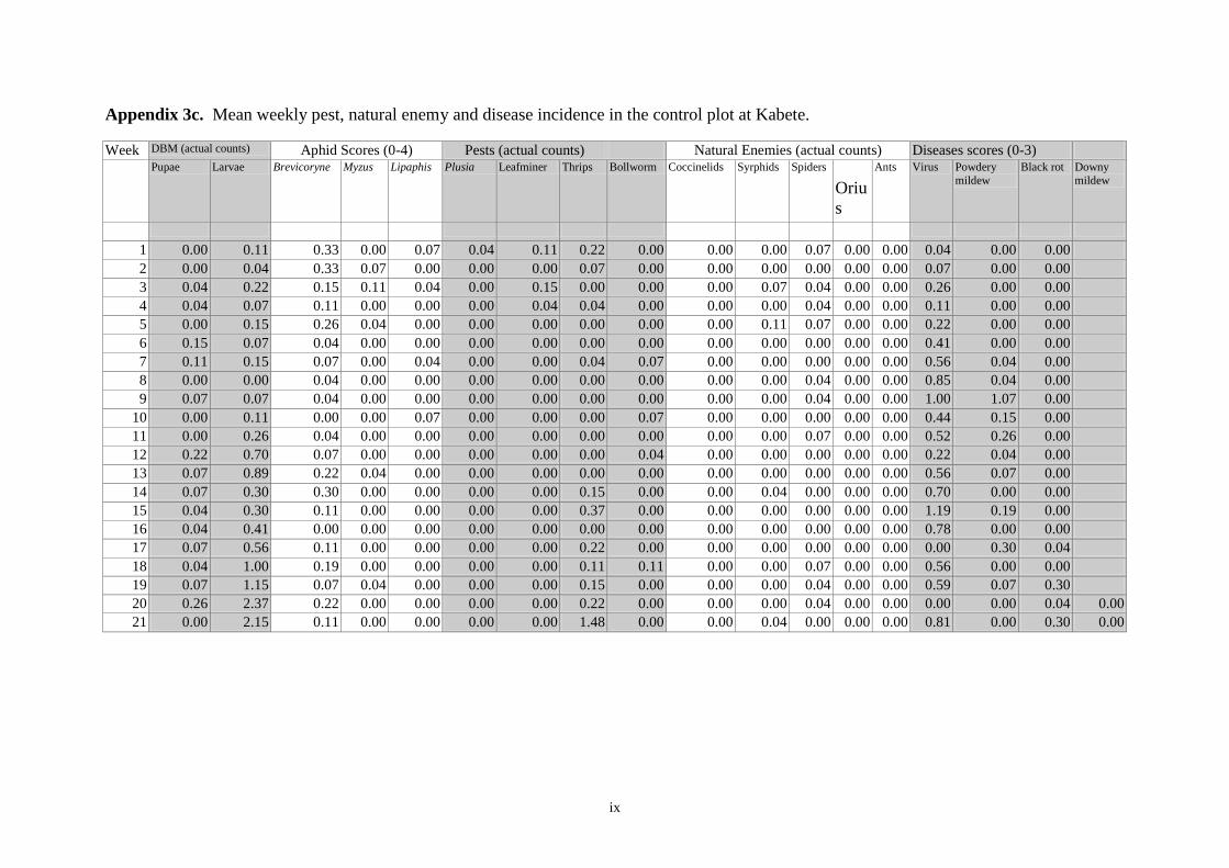
ix

Appendix 3c. Mean weekly pest, natural enemy and disease incidence in the control plot at Kabete.



Oriu

s

Ants Virus Powdery

mildew

Black rot Downy

mildew

1 0.00 0.11 0.33 0.00 0.07 0.04 0.11 0.22 0.00 0.00 0.00 0.07 0.00 0.00 0.04 0.00 0.00

2 0.00 0.04 0.33 0.07 0.00 0.00 0.00 0.07 0.00 0.00 0.00 0.00 0.00 0.00 0.07 0.00 0.00

3 0.04 0.22 0.15 0.11 0.04 0.00 0.15 0.00 0.00 0.00 0.07 0.04 0.00 0.00 0.26 0.00 0.00

4 0.04 0.07 0.11 0.00 0.00 0.00 0.04 0.04 0.00 0.00 0.00 0.04 0.00 0.00 0.11 0.00 0.00

5 0.00 0.15 0.26 0.04 0.00 0.00 0.00 0.00 0.00 0.00 0.11 0.07 0.00 0.00 0.22 0.00 0.00

6 0.15 0.07 0.04 0.00 0.00 0.00 0.00 0.00 0.00 0.00 0.00 0.00 0.00 0.00 0.41 0.00 0.00

7 0.11 0.15 0.07 0.00 0.04 0.00 0.00 0.04 0.07 0.00 0.00 0.00 0.00 0.00 0.56 0.04 0.00

8 0.00 0.00 0.04 0.00 0.00 0.00 0.00 0.00 0.00 0.00 0.00 0.04 0.00 0.00 0.85 0.04 0.00

9 0.07 0.07 0.04 0.00 0.00 0.00 0.00 0.00 0.00 0.00 0.00 0.04 0.00 0.00 1.00 1.07 0.00

10 0.00 0.11 0.00 0.00 0.07 0.00 0.00 0.00 0.07 0.00 0.00 0.00 0.00 0.00 0.44 0.15 0.00

11 0.00 0.26 0.04 0.00 0.00 0.00 0.00 0.00 0.00 0.00 0.00 0.07 0.00 0.00 0.52 0.26 0.00

12 0.22 0.70 0.07 0.00 0.00 0.00 0.00 0.00 0.04 0.00 0.00 0.00 0.00 0.00 0.22 0.04 0.00

13 0.07 0.89 0.22 0.04 0.00 0.00 0.00 0.00 0.00 0.00 0.00 0.00 0.00 0.00 0.56 0.07 0.00

14 0.07 0.30 0.30 0.00 0.00 0.00 0.00 0.15 0.00 0.00 0.04 0.00 0.00 0.00 0.70 0.00 0.00

15 0.04 0.30 0.11 0.00 0.00 0.00 0.00 0.37 0.00 0.00 0.00 0.00 0.00 0.00 1.19 0.19 0.00

16 0.04 0.41 0.00 0.00 0.00 0.00 0.00 0.00 0.00 0.00 0.00 0.00 0.00 0.00 0.78 0.00 0.00

17 0.07 0.56 0.11 0.00 0.00 0.00 0.00 0.22 0.00 0.00 0.00 0.00 0.00 0.00 0.00 0.30 0.04

18 0.04 1.00 0.19 0.00 0.00 0.00 0.00 0.11 0.11 0.00 0.00 0.07 0.00 0.00 0.56 0.00 0.00

19 0.07 1.15 0.07 0.04 0.00 0.00 0.00 0.15 0.00 0.00 0.00 0.04 0.00 0.00 0.59 0.07 0.30

20 0.26 2.37 0.22 0.00 0.00 0.00 0.00 0.22 0.00 0.00 0.00 0.04 0.00 0.00 0.00 0.00 0.04 0.00

21 0.00 2.15 0.11 0.00 0.00 0.00 0.00 1.48 0.00 0.00 0.04 0.00 0.00 0.00 0.81 0.00 0.30 0.00

A SECOND APPRAISAL OF THE PHEROMONE MATING-

DISRUPTION TECHNIQUE FOR DIAMOND-BACK MOTH,

PLUTELLA XYLOSTELLA

A Technical Report for Project R7449:

Development of Biorational Brassica IPM in Kenya

DFID Crop Protection Programme

M.C.A. Downham

Natural Resources Institute, Medway University Campus, University of

Greenwich, Chatham, Kent ME4 4TB, United Kingdom

Collaborating Institutions:

Natural Resources Institute, UK

KARI, National Agricultural Research Laboratories, Kenya

CABI International, Africa Regional Centre, Kenya

ii

Contents

Executive Summary 1

Acknowledgements 2

Introduction 3

Materials and Methods 5

Location and duration of the trial 5

Crops and agronomic practices 5

Trial design and treatments 6

Monitoring of pheromone trap catches 7

Assessments of mating rates 7

Pest sampling and damage assessment 8

Harvesting 9

Quantitative analysis of the Selibate™ dispensers 9

Data analysis 9

Results 10

Pheromone trap catches 10

Mating assessments 12

Weekly DBM and leaf damage counts 13

Non DBM counts 15

Harvests 16

Quantitative analysis of Selibate dispensers 18

Discussion 21

Conclusions 23

References 24

Appendices 26

1

Executive Summary

A trial of pheromone mating disruption of diamondback moth (DBM), Plutella xylostella, L.

was carried out at the Jomo Kenyatta University of Agriculture and Technology farm near

Nairobi, Kenya from October 2001 to January 2002. Following an earlier trial in 2000, this

trial incorporated a number of changes to design and methodology that were intended to

improve treatment effectiveness as well as evaluation of results. The synthetic pheromone

formulation used was a PVC-based one known as 'Selibate' and individual dispensers were

set out at a density of approximately 1425 ha-1

in treated plots. The trial consisted of six

0.1 ha plots of kale, three treatment and three untreated controls, in a randomised-block

design. In the treated plots, mating-disruption dispensers were distributed over an area of a

0.2 ha centred on the kale plot, i.e. there was an unplanted, but treated 'buffer zone' of 6.6 m

around each treated plot. The rate of application of the active ingredient was 110 g ha-1

. No

pesticide applications were made in any of the plots. As determined by weekly sampling,

populations of DBM larvae were generally higher than in the previous trial. There were

slightly fewer larvae in treatment plots and leaf damage scores were consistently slightly

lower; total marketable yield from 6 harvest dates was 50% higher. However these

differences were not statistically significant. Four separate sets of observations to determine

rates of mating of female DBM indicated that the pheromone treatment did not suppress

mating as envisaged. Pheromone trap monitoring showing incomplete suppression of catches

in the pheromone-treated plots, even in the early stages of the trial, strengthened this

conclusion. Quantitative analysis of pheromone dispensers exposed under field conditions

indicated that the half-life of the pheromone within the dispensers was about eight weeks.

Even if mating-disruption of DBM was effective early in the trial, it would have been weak

or absent after this period. The fact that between-treatment differences in DBM larval

numbers, damage scores and marketable yield continued until the end of the trial lends

further weight to the conclusion that these apparent beneficial effects were due to non-

treatment related effects. These results reinforce earlier conclusions that pheromone mating-

disruption of DBM in the context of small-holder farmers in Kenya is not feasible, and future

trials could only possibly succeed if it were practical to increase plot sizes, unit-area dose

rates and physical isolation of plots.

2

Acknowledgements

I fully acknowledge the assistance of Dr G. Oduor and Mr W. Okello Ogutu from CABI-

ARC, and Dr G.N. Kibata and Mr D. Miano of KARI who set-up and managed the trial at the

Jomo Kenyatta University of Agriculture and Technology. Field teams from both

organisations worked tirelessly to ensure its smooth running and Messrs Okello Ogutu and

Miano were instrumental in this. I am also very grateful for the assistance of Mr M. Kaibui

(Assistant Farm Manager) at JKUAT, who was immensely helpful in managing the trial

plots. I thank Mark Parnell (NRI), Denis Djegui (IITA, Cotonou) and David Woodward

(Horticulture Research International) for field assistance while setting up the trial, Mrs

Margaret Brown (NRI) for procurement assistance, Dudley Farman (NRI) for laboratory

analysis of mating disruption dispensers and Dr Jane Poole (CABI-ARC) for useful statistical

advice.

This publication is an output from project R7449 funded by the Crop Protection Programme

of the United Kingdom Department for International Development (DFID) for the benefit of

developing countries. The views expressed are not necessarily those of DFID.

3

Introduction

Project R7449 aims to develop, evaluate and promote two new biologically based IPM

control methods for the diamond-back moth (DBM), Plutella xylostella, L. on small-holder

vegetable farms in Kenya. These are the use of pheromone-based mating-disruption and an

endemic viral bio-pesticide. This report details results from the second of two trials of

pheromone mating-disruption for management of DBM. Results of the first trial in 2000,

together with a discussion of earlier trials in Kenya (Critchley et al., 1998, 1999a, 1999b) and

elsewhere, were reported previously (Downham, 2001).

The first trial was carried out at three sites near Nairobi, Kenya from March to August 2000.

The synthetic pheromone formulation used was a PVC-based one known as 'Selibate' and

individual dispensers were set out at a density of approximately 625 ha-1

. At each site single,

0.1 ha plots of kale containing 60 and 120 g ha-1

of pheromone active ingredient were

compared with a control plot. One or two aphicide sprays were made early in the season in

all plots, but controls were otherwise untreated. As determined by weekly sampling,

populations of pests, including DBM, were low throughout the trial and no clear between-

treatment differences in the numbers of DBM larvae and pupae, or in yield, were observed.

Pheromone trap monitoring indicated incomplete suppression of catches in the pheromone-

treated plots, even in the early stages of the trial, when disruption of pheromone-mediated

behaviour should have been greatest.

From the results of the first trial it was concluded that the pheromone treatments had not

disrupted mating of DBM. Earlier, apparently successful, results in Kenya may have been

due to insecticide 'resurgence' effects in control plots providing a favourable, but misleading,

comparison with the pheromone plots. Through a comparison of trial results from Japan and

the US, which involved much higher application rates and/or greater plot sizes, it was further

concluded that the only chance of successful mating disruption in the Kenyan, small-holder

farmer context lay in increasing pheromone dispenser density and effective plot size. Based

on this and other conclusions, several recommendations were made. These, and some other

changes, were incorporated in the second trial although much of the basic methodology

remained the same.

4

Three important changes in the second trial were:

a doubling of pheromone dispenser density (while using the higher of the two

application rates from the first trial);

deployment of pheromone dispensers, not only within the planted area, but in 'buffer-

zone' around it, effectively doubling the area covered;

using a lower dispenser height (~ 50 cm, compared to 1 m).

The aim of these changes was to create a denser and more homogenous cloud of pheromone

within the crop and thus increase its effectiveness.

Another significant alteration was that the trial should consist of replicated control and

treatment plots, at a single site, thus allowing analysis of variance to be employed in the

statistical evaluation of results. Equally importantly, direct methods of assessing mating of

female DBM within plots were used for the first time in Kenya. This was to determine

directly whether the envisaged mode of action of the treatments – suppression of mating –

was actually occurring. Finally, a more thorough quantitative analysis of pheromone in

dispensers was carried out to determine the amounts of pheromone remaining in the

dispensers through time – and hence their effective longevity.

5


Location and duration of trial

The trial was conducted in three fields at the Jomo Kenyatta University of Agriculture and

Technology farm site (JKUAT), situated about 24 km north-east of Nairobi. It began on 8

October 2001 and ran until 28 January 2002.

Crops and agronomic practices

The target crop was kale (Collard var. Southern Georgia), Brassica oleracea. All plants were

transplanted into the plots as seedlings with 3 – 6 true leaves at a spacing of 60 60 cm.

Seedlings came from field nursery beds sown at JKUAT on 4 September 2001 for the trial.

Transplanting took place on 8 October. Due to dry weather all plots were irrigated using

overhead irrigation equipment, for at least two weeks following transplanting, and thereafter

were rain-fed. Despite this, some seedlings died, necessitating gap-filling which was carried

out on a piecemeal basis for about 2 weeks after initial transplanting.

Fertiliser applications and weeding were carried out as indicated in Table 1 below. No

insecticide applications were made in any of the plots.

Table 1. Dates of fertiliser applications and weeding during the trial.

Operation Dates Details

Fertiliser applications 8 October (transplanting) DAP1, 5 g per plant hill

31 October CAN2, 10 g per plant hill

3 December CAN, 10 g per plant hill

Weeding 30 October

14 November

27 November

14 December

29 December

12 January 1Diammonium Phosphate.

2Calcium Ammonium Nitrate.

6

Trial design and treatments

The trial consisted of three pheromone treated plots of kale and three untreated controls. A

'blocked' trial design was achieved by positioning one treated and one control plot in each of

three separate, rectangular-shaped fields, varying in area from 0.7 to 1.6 ha. In order to avoid

pheromone-mediated interactions between plots, plots within each field were positioned at

least 50 m apart at opposite ends of the respective fields. Maize was subsequently planted in

20 – 30 m wide strips in the middle portion of each field to act as a further barrier to pest and

pheromone movement between plots.

Individual plots planted to kale were 0.10 ha in area; dimensions of those in blocks 1 and 3

were 31.8 31.8 m; in block 2 they were 20 50 m. However, with the treated plots the

areas covered by pheromone dispensers extended beyond the plot boundaries by 6.6 m in

each dimension to cover an area of slightly more than 0.2 ha in each case.

The pheromone formulation used was the same as that for the previous trial, in 2000, i.e. a

black, PVC „shoelace‟ or Selibate™ formulation (Cork et al., 1989) produced by Agrisense-

BCS, Pontypridd, UK in August 2001. This contained a blend of (Z)-11-hexadecenal, (Z)-11-

hexadeceny acetate and (Z)-11-hexadecenol in the ratio 55:45:1, with a total active ingredient

content of 7.6 mg g-1

(determined by analysis at NRI). The departure of the blend from the

nominal 50:50:1 ratio was not considered to be biologically significant.

The pheromone formulation was applied on 11 October. Individual lengths weighing 1 g were

fixed into the split top end of bamboo canes, at a height of 0.5 m, and these were positioned 2.78

m apart in a grid pattern. This produced a density of approximately 1425 sources ha-1

and a

pheromone application rate of 110 g a.i. ha-1

. Due to differing plot dimensions the actual

numbers of dispensers per treatment plot were 289 (blocks 1 and 3) and 299 (block 2).

Dispensers that were damaged or lost during the course of the trial were replaced with fresh

dispensers within a few days.

7

Monitoring of pheromone trap catches

Daily catches of adult male DBM in three white, sticky-delta pheromone traps placed in each

plot were recorded. The traps were baited with polyethylene vial lures (23 mm × 9 mm

diameter) containing 0.1 mg (Z)-11-16:Ald, (Z)-11-16:Ac and (Z)-11-16:OH in the respective

ratio of 50:50:1, plus 0.2 mg BHT. Sticky card trap inserts were replaced weekly; pheromone

lures were replaced every two weeks. Traps and lures were supplied by International

Pheromone Systems, Wirral, U.K. Traps were set out on 11 October 2001.

Assessments of mating rates

Mating rates of adult female DBM were assessed by four different methods. Firstly, the

method of Ohno et al. (1992) was adapted as follows. One to 2 day-old virgin females from

the KARI culture were tethered by one wing using white cotton thread, then placed in plots

between 5 and 7 pm. The loose end of the thread was secured between the plastic pot used for

transportation (10 cm diameter × 4 cm deep) and its lid; females were positioned on kale

seedlings 4 – 5 m apart in a central region of plots. They were retrieved between 7.00 and

8.30 am the following morning. This procedure was carried out three times, when between 24

and 39 females were placed on each occasion (4 – 7 females per plot).

The following methodology was adapted from Schroeder et al. (2000). The wings of 1 – 2

day-old virgin females from the KARI culture were clipped. The females were left overnight

in plots in plastic containers (21 11 cm, by 5 cm deep) whose inner walls are painted with

fluon to prevent escape. The containers were open to the air and placed on the ground. This

was carried out twice, with 60 females set out (10 per plot) on each occasion. As with the

tethered females, they were placed in plots in the early evening and collected the following

morning.

Wild females were also collected from plots on three occasions (10 – 12 per plot collected

between 6 and 7pm). Once collected from plots the tethered, clipped-wing and wild females

were returned to KARI laboratories and maintained individually in plastic containers with

access to honey solution and pieces of fresh kale leaves, which were replaced daily. The

8

leaves were checked regularly for the presence of larvae for up to 2 weeks. Individuals

producing viable eggs were considered to have mated.

A fourth, and less direct, assessment method was employed on four occasions. In addition to

the standard pheromone traps with synthetic lures, a further three sticky, delta traps were

positioned per plot, each containing virgin females from the KARI culture. Females were

confined to containers made of 3 – 4 cm lengths of polythene hose suspended within the

traps. The open ends of the tubes were covered with gauze, allowing some airflow through

the tube. The tubes were positioned such that their long axes were parallel to that of the trap.

On the first two occasions, 16 – 17 October and 11 – 12 November, two females were trap

were used and thereafter four females per trap. Females were 1 – 2 days old, except on the

first occasion when they were 3 – 4 days old. Captures of males in the traps were recorded in

the usual way.

Pest sampling and damage assessment

DBM and other invertebrates and diseases were sampled on a weekly basis from 28 plants in

each plot beginning on 22 October (11 days after transplanting) and ending on 28 January.

Seven groups of four plants each were sampled in each plot, as follows. A single plant was

randomly selected from within each plot (excluding the outer two rows). Sampling was

carried out on this plant and three adjacent ones to the front and right of the randomly

selected plant, as viewed from a consistent direction. If a plant was missing, another adjacent

plant was sampled instead. All invertebrates on sampled plants were counted individually,

except for aphids. Aphid species, plant diseases and leaf damage were scored by visual

inspection as indicated in the Table 2.

Table 2. Scoring system used for sampling of aphids, plant diseases and leaf damage.

Score

Aphid species (top-most,

fully expanded leaf only)

Diseases (whole plant) Leaf Damage (whole plant)

0 no aphids present no symptoms no symptoms

1 ~5% of leaf area covered ≤10% of plant affected ≤10% of leaf area affected

2 ~10% “ “ 11 - 50% “ “ 11 - 50% “ “ “

3 ~25% “ “ ≥50% “ “ ≥50% “ “ “

4 ≥50% “ “ - -

9

Harvesting

Harvesting commenced on 12 November (4 weeks after transplanting) in all plots then

continued at 2-week intervals until 21 January, making 6 harvests in all. On each occasion the

total number of marketable and damaged leaves, and their weight, was recorded separately,

together with a count of the plant stand in each plot.

Quantitative analysis of the Selibate dispensers

Quantitative analysis of the mating-disruption formulation was carried out in order to

determine the amount of pheromone remaining in dispensers through the course of the

season. On 11 October (day 0), 60 dispensers were placed on a group of canes (two

dispensers per cane) on the JKUAT farm more than 50 m from the nearest experimental plots.

On day 0, day 11 then subsequently every seven days until 21 January, three randomly

selected dispensers were removed from the sticks. These were wrapped in aluminium foil

and placed in a fridge, until sent back to NRI in late January for laboratory analysis. The

amount of each pheromone component contained in three sub-sample lengths of the

formulation from each date was determined and compared to day 0 samples.

Data analysis

Most data sets considered hereafter were subjected to one-way analysis of variance (with

blocking) (ANOVA) using Genstat 5 (Release 4.1) for Windows™. Where significant

treatment effects were indicated this was confirmed by calculation of the appropriate least

significant difference (5% level).

For trap-catch data (synthetic lures) the mean catch per trap in each plot, for successive weekly

periods, was first calculated. From these values, the mean weekly catch per trap, for the first

eight weeks and throughout the trial, was calculated for each plot and these values subjected to

ANOVA. The period of eight weeks related to the expected effective longevity of the mating-

disruption dispensers and this point is considered more fully in the Discussion.

Similarly for pest sampling and damage data, the mean value (of 28 plants) for each plot was

first determined for each sample date; the mean value for all sample dates, and for sample dates

up to week 8, were then calculated for each plot and subjected to ANOVA. Yield data from

each harvest date, for each plot, were adjusted for plant stand differences by multiplying by the

factor (initial plant stand count/plant stand count at harvest). Adjusted yield data were then

summed across the first three sample harvests and for all harvest dates, and total yield data

values used in respective ANOVAs. Mating assessment data from wild, caught females and

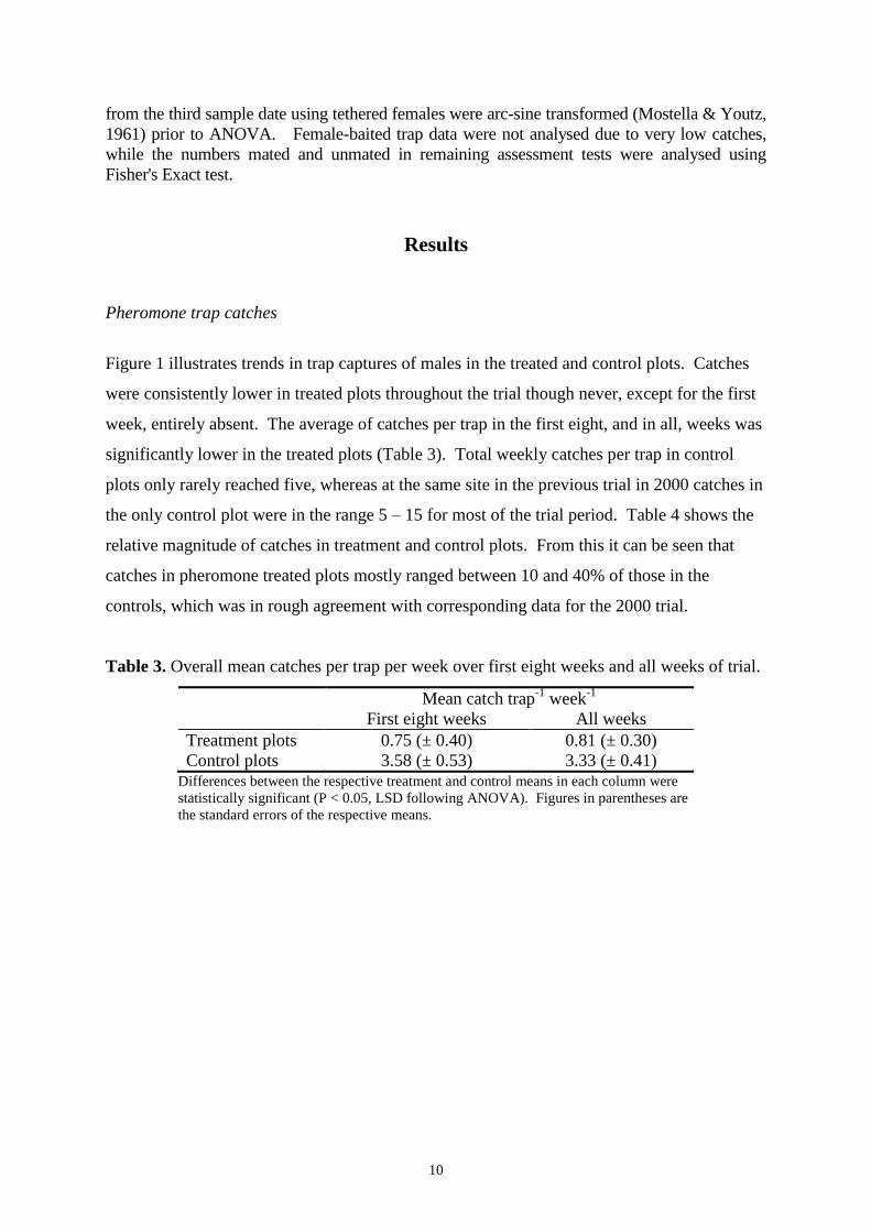
10

from the third sample date using tethered females were arc-sine transformed (Mostella & Youtz,

1961) prior to ANOVA. Female-baited trap data were not analysed due to very low catches,

while the numbers mated and unmated in remaining assessment tests were analysed using

Fisher's Exact test.

Results

Pheromone trap catches

Figure 1 illustrates trends in trap captures of males in the treated and control plots. Catches

were consistently lower in treated plots throughout the trial though never, except for the first

week, entirely absent. The average of catches per trap in the first eight, and in all, weeks was

significantly lower in the treated plots (Table 3). Total weekly catches per trap in control

plots only rarely reached five, whereas at the same site in the previous trial in 2000 catches in

the only control plot were in the range 5 – 15 for most of the trial period. Table 4 shows the

relative magnitude of catches in treatment and control plots. From this it can be seen that

catches in pheromone treated plots mostly ranged between 10 and 40% of those in the

controls, which was in rough agreement with corresponding data for the 2000 trial.

Table 3. Overall mean catches per trap per week over first eight weeks and all weeks of trial.

Mean catch trap-1

week-1

First eight weeks All weeks

Treatment plots 0.75 (± 0.40) 0.81 (± 0.30)

Control plots 3.58 (± 0.53) 3.33 (± 0.41) Differences between the respective treatment and control means in each column were

statistically significant (P < 0.05, LSD following ANOVA). Figures in parentheses are

the standard errors of the respective means.

11

Figure 1. Mean weekly trap-catches in pheromone treated and control plots (error bars

indicate standard errors of the respective means).

Table 4. Mean weekly trap-catches in the pheromone plots expressed as a percentage of

those in the control plots.

Week Ending Treatment as %

of Control

1 18-Oct-01 0.0

2 25-Oct-01 6.8

3 1-Nov-01 20.0

4 8-Nov-01 8.8

5 15-Nov-01 17.6

6 22-Nov-01 38.0

7 29-Nov-01 34.5

8 6-Dec-01 41.2

9 13-Dec-01 16.2

10 20-Dec-01 12.9

11 27-Dec-01 22.7

12 3-Jan-02 30.8

13 10-Jan-02 45.5

14 17-Jan-02 14.7

15 24-Jan-02 61.5

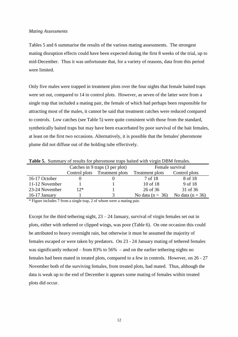
12

Mating Assessments

Tables 5 and 6 summarise the results of the various mating assessments. The strongest

mating disruption effects could have been expected during the first 8 weeks of the trial, up to

mid-December. Thus it was unfortunate that, for a variety of reasons, data from this period

were limited.

Only five males were trapped in treatment plots over the four nights that female baited traps

were set out, compared to 14 in control plots. However, as seven of the latter were from a

single trap that included a mating pair, the female of which had perhaps been responsible for

attracting most of the males, it cannot be said that treatment catches were reduced compared

to controls. Low catches (see Table 5) were quite consistent with those from the standard,

synthetically baited traps but may have been exacerbated by poor survival of the bait females,

at least on the first two occasions. Alternatively, it is possible that the females' pheromone

plume did not diffuse out of the holding tube effectively.

Table 5. Summary of results for pheromone traps baited with virgin DBM females.

Catches in 9 traps (3 per plot) Female survival

Control plots Treatment plots Treatment plots Control plots

16-17 October 0 0 7 of 18 8 of 18

11-12 November 1 1 10 of 18 9 of 18

23-24 November 12* 1 26 of 36 31 of 36

16-17 January 1 3 No data (n = 36) No data (n = 36) * Figure includes 7 from a single trap, 2 of whom were a mating pair.

Except for the third tethering night, 23 – 24 January, survival of virgin females set out in

plots, either with tethered or clipped wings, was poor (Table 6). On one occasion this could

be attributed to heavy overnight rain, but otherwise it must be assumed the majority of

females escaped or were taken by predators. On 23 - 24 January mating of tethered females

was significantly reduced – from 83% to 56% – and on the earlier tethering nights no

females had been mated in treated plots, compared to a few in controls. However, on 26 - 27

November both of the surviving females, from treated plots, had mated. Thus, although the

data is weak up to the end of December it appears some mating of females within treated

plots did occur.

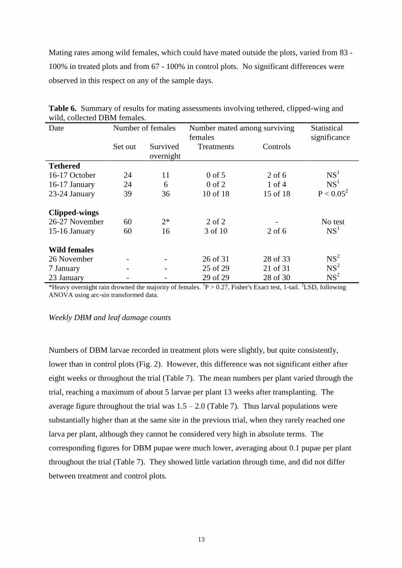
13

Mating rates among wild females, which could have mated outside the plots, varied from 83 -

100% in treated plots and from 67 - 100% in control plots. No significant differences were

observed in this respect on any of the sample days.

Table 6. Summary of results for mating assessments involving tethered, clipped-wing and

wild, collected DBM females.

Date Number of females Number mated among surviving

females

Statistical

significance

Set out Survived

overnight

Treatments Controls

Tethered

16-17 October 24 11 0 of 5 2 of 6 NS1

16-17 January 24 6 0 of 2 1 of 4 NS1

23-24 January 39 36 10 of 18 15 of 18 P < 0.052

Clipped-wings

26-27 November 60 2* 2 of 2 - No test

15-16 January 60 16 3 of 10 2 of 6 NS1

Wild females

26 November - - 26 of 31 28 of 33 NS2

7 January - - 25 of 29 21 of 31 NS2

23 January - - 29 of 29 28 of 30 NS2

*Heavy overnight rain drowned the majority of females. 1P > 0.27, Fisher's Exact test, 1-tail. 2

LSD, following

ANOVA using arc-sin transformed data.

Weekly DBM and leaf damage counts

Numbers of DBM larvae recorded in treatment plots were slightly, but quite consistently,

lower than in control plots (Fig. 2). However, this difference was not significant either after

eight weeks or throughout the trial (Table 7). The mean numbers per plant varied through the

trial, reaching a maximum of about 5 larvae per plant 13 weeks after transplanting. The

average figure throughout the trial was 1.5 – 2.0 (Table 7). Thus larval populations were

substantially higher than at the same site in the previous trial, when they rarely reached one

larva per plant, although they cannot be considered very high in absolute terms. The

corresponding figures for DBM pupae were much lower, averaging about 0.1 pupae per plant

throughout the trial (Table 7). They showed little variation through time, and did not differ

between treatment and control plots.

14

Figure 2. Mean number of DBM larvae per plant in pheromone treated and control plots

(error bars indicate standard errors of the respective means).

Table 7. Mean numbers of DBM larvae and pupae per plant sampled over first eight and all

weeks of the trial.

Mean larvae plant-1

Mean pupae plant-1

First 8 weeks All weeks First 8 weeks All weeks

Treatment plots 1.41 (± 0.32) 1.62 (± 0.10) 0.11 (± 0.05) 0.12 (± 0.02)

Control plots 1.83 (± 0.51) 1.92 (± 0.19) 0.10 (± 0.02) 0.10 (± 0.02) Differences between the respective treatment and control means in each column were not statistically significant

(P > 0.25, F-ratio of ANOVA). Figures in parentheses are the standard errors of the respective means.

Leaf damage scores in the first 2 – 3 weeks of the trial were very low, but rose steadily to a

maximum of around 1.0 (on a scale of 0 – 3) at around 8 – 9 weeks after transplanting

(Fig. 3). A score of 1.0 indicated a maximum of 10% of leaf area missing or damaged and

thus equated to relatively little damage. Damage scores tended to be slightly lower in

treatment plots compared to controls on most sample dates. The difference averaged over the

first eight weeks of the trial was not statistically significant; however, that averaged over all

weeks was significant (Table 8).

15

Table 8. Mean leaf damage scores over first eight and all weeks of trial.

Mean damage score

First eight weeks All weeks

Treatment plots 0.54 (± 0.07) 0.72 (± 0.03)

Control plots 0.67 (± 0.13) 0.77 (± 0.03) The difference between the treatment and control means for the first 8 weeks was not

statistically significant (P = 0.18, F-ratio of ANOVA), while that for all weeks was

significant (P < 0.05, LSD following ANOVA). Figures in parentheses are the standard

errors of the respective means.

Figure 3. Mean leaf damage score (scale 0 – 3) per plant in pheromone treated and control

plots (error bars indicate standard errors of the respective means).

Non-DBM counts

Comprehensive tables of invertebrate and disease incidence are given in Appendices 1a - b,

2a - b and 3a - b.

Aphids and thrips were the only other pests of note, besides DBM, throughout the trial.

Among the aphids, Brevicoryne brassicae was the dominant species but Myzus persicae and

Lipaphis erysimi were also present. Mean B. brassicae scores remained below 0.1 per plant

until 8 weeks after transplanting (scale, 0 – 4) then increased sharply to reached 0.5 per plant

by the end of the trial. Aphid scores did not differ between treatment and control plots

0.0

0.2

0.4

0.6

0.8

1.0

1.2

1.4

2 3 4 5 6 7 8 9 10 11 12 13 14 15 16

weeks after transplanting

me

an

da

ma

ge

sc

ore

Treatment

Control

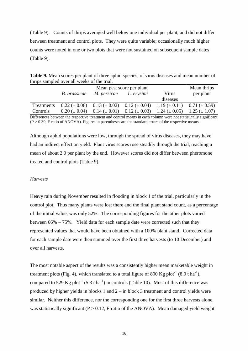
16

(Table 9). Counts of thrips averaged well below one individual per plant, and did not differ

between treatment and control plots. They were quite variable; occasionally much higher

counts were noted in one or two plots that were not sustained on subsequent sample dates

(Table 9).

Table 9. Mean scores per plant of three aphid species, of virus diseases and mean number of

thrips sampled over all weeks of the trial.

Mean pest score per plant Mean thrips

per plant B. brassicae M. persicae L. erysimi Virus

diseases

Treatments 0.22 (± 0.06) 0.13 (± 0.02) 0.12 (± 0.04) 1.19 (± 0.11) 0.71 (± 0.59)

Controls 0.20 (± 0.04) 0.14 (± 0.01) 0.12 (± 0.03) 1.24 (± 0.05) 1.25 (± 1.07) Differences between the respective treatment and control means in each column were not statistically significant

(P > 0.39, F-ratio of ANOVA). Figures in parentheses are the standard errors of the respective means.

Although aphid populations were low, through the spread of virus diseases, they may have

had an indirect effect on yield. Plant virus scores rose steadily through the trial, reaching a

mean of about 2.0 per plant by the end. However scores did not differ between pheromone

treated and control plots (Table 9).

Harvests

Heavy rain during November resulted in flooding in block 1 of the trial, particularly in the

control plot. Thus many plants were lost there and the final plant stand count, as a percentage

of the initial value, was only 52%. The corresponding figures for the other plots varied

between 66% – 75%. Yield data for each sample date were corrected such that they

represented values that would have been obtained with a 100% plant stand. Corrected data

for each sample date were then summed over the first three harvests (to 10 December) and

over all harvests.

The most notable aspect of the results was a consistently higher mean marketable weight in

treatment plots (Fig. 4), which translated to a total figure of 800 Kg plot-1

(8.0 t ha-1

),

compared to 529 Kg plot-1

(5.3 t ha-1

) in controls (Table 10). Most of this difference was

produced by higher yields in blocks 1 and 2 – in block 3 treatment and control yields were

similar. Neither this difference, nor the corresponding one for the first three harvests alone,

was statistically significant (P > 0.12, F-ratio of the ANOVA). Mean damaged yield weight

17

was similar in treatment and control plots; thus total yield was greater in treatment plots but

this effect was also not significant (Table 10).

Figure 4. Mean weight of marketable yield per 0.1 ha plot (in Kg) in pheromone treated and

control plots on successive harvest dates (error bars indicate standard errors of the respective

means).

Table 10. Mean weight of damaged, marketable and total yields per 0.1 ha plot in first three

and all harvests combined (all data following correction to 100% plant stand).

Yield harvested (Kg plot-1

)

Damaged Marketable Total

First 3 Harvests

Treatments 180.9 (± 68.7) 346.1 (± 117.3) 527.0 (± 162.6)

Controls 177.5 (± 55.3) 211.7 (± 66.3) 389.2 (± 96.8)

P for differences* 0.82 0.13 0.17

All Harvests

Treatments 622.4 (± 131.2) 799.7 (± 258.0) 1422.1 (± 364.7)

Controls 612.3 (± 99.5) 529.1 (± 148.5) 1141.4 (± 242.9)

P for differences* 0.81 0.14 0.16 *P is for the F-ratio of the relevant ANOVA. Figures in parentheses are the standard errors of the

respective means.

Paralleling the marketable weight, the mean number of marketable leaves was greater in

treatment plots. Although this difference was not significant in respect of the first three

18

harvests or all harvests, there were significantly more damaged leaves in control plots over

both periods (Table 11).

Table 11. Mean number of damaged and marketable leaves and their total per 0.1 ha plot in

first three and all harvests combined (all data following correction to 100% plant stand).

Number of leaves harvested

Damaged Marketable Total

First 3 Harvests

Treatments 15546 (± 3585) 19806 (± 4713) 35352 (± 5384)

Controls 18905 (± 3876) 15048 (± 2841) 33953 (± 3966)

P for differences* 0.05 0.14 0.54

All Harvests

Treatments 39898 (± 4898) 40064 (± 8908) 79961 (± 9554)

Controls 46540 (± 3963) 32528 (± 6124) 79068 (± 8230)

P for differences* < 0.01 0.13 0.64 *P is for the F-ratio of the relevant ANOVA. Figures in parentheses are the standard errors of the respective

means.

Quantitative analysis of Selibate™ dispensers

Analysis of the unexposed (day 0) Selibate™ dispensers showed that the original

concentration of pheromone active ingredient within the formulation was 8.6% – slightly

higher than the intended figure of 8% (Table 12). Initially the proportion of the Z11-16:Ac

pheromone component was about 44% of the total, and that of Z11-16:Ald about 56% – in

contrast to the intended 50:50 ratio. However, as expected Z11-16:Ac was more persistent so

that the actual ratio of these two major components was close to 50:50 for the first 50 – 60

days of the trial.

Figure 5 shows the total pheromone remaining at each sample date, as a percentage of the

amount at day 0. From this it can be seen that on the last sample date (21 January), 102 days

after setting out the dispensers, the amount of total pheromone remaining was approximately

30% of the day 0 value. The data show an exponential decline in pheromone remaining, that

would have been reflected in the amount released per unit time. The data are well fitted3 (F-

ratio = 492.0, ANOVA of the regression model, model d.f.=2, residual d.f.=13, P < 0.001) by

the equation:

3 Note that the fit of the linear relation, Y = 86.1 - 0.6X, to the data while also significant, is poorer (c.f. F-ratio

= 96.6, ANOVA of the regression model) than the exponential.

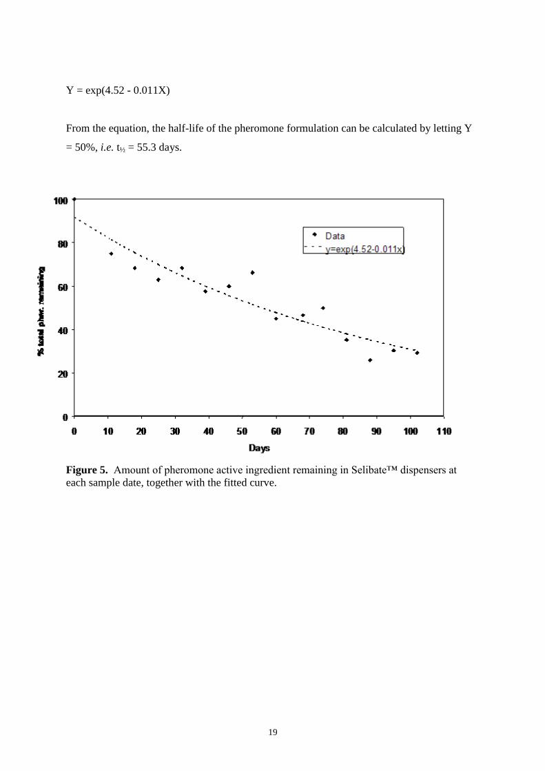
19

Y = exp(4.52 - 0.011X)

From the equation, the half-life of the pheromone formulation can be calculated by letting Y

= 50%, i.e. t½ = 55.3 days.

Figure 5. Amount of pheromone active ingredient remaining in Selibate™ dispensers at

each sample date, together with the fitted curve.

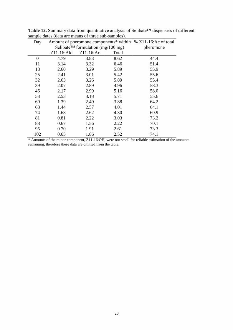
20

Table 12. Summary data from quantitative analysis of Selibate™ dispensers of different

sample dates (data are means of three sub-samples).

Day Amount of pheromone components* within

Selibate™ formulation (mg/100 mg)

% Z11-16:Ac of total

pheromone

Z11-16:Ald Z11-16:Ac Total

0 4.79 3.83 8.62 44.4

11 3.14 3.32 6.46 51.4

18 2.60 3.29 5.89 55.9

25 2.41 3.01 5.42 55.6

32 2.63 3.26 5.89 55.4

39 2.07 2.89 4.96 58.3

46 2.17 2.99 5.16 58.0

53 2.53 3.18 5.71 55.6

60 1.39 2.49 3.88 64.2

68 1.44 2.57 4.01 64.1

74 1.68 2.62 4.30 60.9

81 0.81 2.22 3.03 73.2

88 0.67 1.56 2.22 70.1

95 0.70 1.91 2.61 73.3

102 0.65 1.86 2.52 74.1 * Amounts of the minor component, Z11-16:OH, were too small for reliable estimation of the amounts

remaining, therefore these data are omitted from the table.

21

Discussion

To put the various measures of effectiveness of the mating-disruption treatment into context,

it is useful, first, to consider the results of the quantitative analysis of the mating-disruption

dispensers. The data of Fig. 5 and Table 12 show that total pheromone remaining in the

dispensers was half of its initial value after about eight weeks. By comparison Critchley et al.

(1998) found that 61 – 70% of pheromone remained in Selibate™ dispensers 64 days after

transplanting. The greater overall longevity in that case may have been related to the

experiment having been undertaken at a different time of year (i.e. during the long rains).

Since the present data show an exponential decline the amount of pheromone released into

the crop per unit time would have fallen in a parallel manner. Moreover, after about eight

weeks the balance of the two major blend components was increasingly skewed away from

the ideal 50:50 ratio. In reality the practical effectiveness of the pheromone treatments would

have declined in a gradual manner, and the fixing of any particular time-frame of

effectiveness is somewhat arbitrary. However, given the results for amount of pheromone

remaining and blend balance, eight weeks seems the maximum period for which good control

of DBM might, theoretically, be possible. It would have been weak or absent thereafter.

From the results there were several small indications of treatment effectiveness, specifically:

slightly lower DBM larval numbers in treatment plots;

slightly leaf damage scores in treatment plots;

higher marketable weights in treatment plots;

lower numbers of damaged leaves in treatment plots.

As noted in the Results section, most of these effects were not statistically significant, but

their consistent occurrence through the trial is nevertheless suggestive of a slight controlling

effect of the pheromone treatment. To weigh this possibility, against the alternative one that

lower DBM populations/higher yields (if real) were unrelated to treatment effects, it is

necessary to consider other aspects of the results.

22

Clearly, the best determinant must be the mating assessment data. Although these were

limited for a variety of practical reasons, particularly for the first eight weeks of the trial, it is

possible to draw some conclusions. Combining the tethered- and clipped-wing female data

for October – November, when mating suppression should have been strongest, two of seven

females were mated from treatment plots, compared to two of six from controls. These were

females that must have mated within the plots; the numbers are not indicative of suppression

of mating in the treatment plots. A significant reduction of mating was seen using tethered-

females in late-January. In the author's view this was probably a chance effect, since by then

the mating-disruption dispensers would not have been very effective. In any case more than

half of the females in the treated plot were still mated, so the practical usefulness of the result

is doubtful.

With the female-baited traps, for the period to the end of November, two males were trapped

in treated plots and 13 in controls. However, seven of the latter can be discounted for reasons

noted in the Results section. This result suggests that at least some males were able to locate

females in the treatment plots.

Considering the data for wild females, which were more numerous, it was very clear that

there was no suppression of mating in treatment plots on any of the three sample dates –

including the 26 – 27 November. While it can be argued that many of the females could have

mated outside the plot, then flown in, such an effect is one that would have to be contended

with by any control method. For mating-disruption treatments the only ways it could be

minimised is through the use of large plot sizes and extreme isolation of the plot from other

sources of DBM.

Overall, the mating data indicate that suppression of mating – the envisaged mode of action –

was not occurring in the treatment plots. The catch data for the standard pheromone traps

strengthen this conclusion. If the success of males at locating the traps in the treated plots

was 10 – 40% of that in control plots, as the results show, then at least that proportion of

females (probably more) would have been found and mated by males.

The other way of determining whether the pheromone treatments were having a real

controlling effect is to look at the period over which relevant trends persisted. As argued

above, control through mating suppression would have been strongest during the first eight

23

weeks of the trial and largely absent thereafter. Inspection of Figs. 2 – 4 shows that the

apparently beneficial between-treatment differences in DBM larval populations, leaf damage

and marketable yield did very largely continue through the latter half of the trial. Since the

pheromone treatments could not have been effective at that time, this is good evidence that

the earlier trends were also unrelated to the pheromone treatment.

Conclusions

The results presented and discussed above reinforce the conclusions of the trials carried out in

2000 that:

1. Pheromone mating-disruption of DBM in the context of small-holder farmers in Kenya is

not feasible.

2. Future trials could only succeed if it were practical to increase plot sizes, unit-area dose

rates and, ideally, physical isolation of plots.

24

References

Cork, A., Hall, D.R., Smith, J. & Jones, O.T. (1989). A new resin formulation for controlled

release of insect pheromones. Controlled Release Society Inc. 16th International

Symposium on controlled release of bioactive materials. Chicago, Illinois, U.S.A. August

6-9, 1989.

Critchley, B.R., Farman, D.I., Hall, D.R., Ong'aro, J.M., Kibata, G.N., Olubayo, F., Nbuvi,

J.N., Kaibui, M. & Kamau, C. (1998). Biorational control technologies for the integrated

pest management of diamondback moth, Plutella xylostella, on brassica crops in Kenya. I.

Use of sex pheromones: trap designs, pheromone blends and the optimum rate of

application of a novel slow release formulation for monitoring and communication

disruption. Unpublished report, Natural Resources Institute. 45 pp.


(1999a). Biorational control technologies for the integrated pest management of

diamondback moth, Plutella xylostella, on brassica crops. II. Mating disruption trials

during the major rainy season, May to September 1998. Unpublished report, Natural



(1999b). Biorational control technologies for the integrated pest management of

diamondback moth, Plutella xylostella, on brassica crops. III. Mating disruption trials

during the major dry season, February to April 1999. Unpublished report, Natural


Downham, M.C.A. (2001). An appraisal of the pheromone mating-disruption technique for

management of diamond-back moth, Plutella xylostella. Unpublished report, Natural


Ohno, T., Asayama., T. & Ichikawa, K. (1992). Evaluation of communication disruption

method using synthetic sex pheromone to suppress diamondback moth infestations. In:

Talekar, N.S. (ed.). Diamondback moth and other crucifer pests. Proceedings of the

25

Second International Workshop, Tainin, Taiwan, 10-14 December 1990. Asian

Vegetable Research and Development Center, pp. 109-114.

Schroeder, P.C., Shelton, A.M., Ferguson, C.S., Hoffmann, M.P. & Petzoldt, C.H. (2000).

Application of synthetic sex pheromone for management of diamondback moth, Plutella

xylostella, in cabbage. Entomologia Experimentalis et Applicata 94, 243-248.

26

Executive Summary

Vegetable production in the peri-urban area surrounding Nairobi has expanded over the

years in response to the increasing demand for food from a rapidly growing urban

population. However, the resulting opportunities and constraints to expanded vegetable

production pose new challenges to crop management. The Department for International

Development (DFID), Crop Protection Programme managed by NR International has

invested in research aimed at developing novel pest management technologies for use in

the peri-urban vegetable system. Focusing mainly on the rational use of chemicals and

alternatives to chemicals as a way of controlling vegetable pests and diseases, this

research has been guided by a perceived existing demand. A key finding in an earlier

demand assessment for alternative pest management technologies revealed that whilst

pest and diseases are the most important production constraint, there was widespread

misuse of chemical pesticides by farmers. The survey presented here attempts to

characterize the peri-urban vegetable production system in order to identify the specific

farmer characteristics, and investigates more closely the perceived pest problems that lead

to the current production practices. The survey was carried out on 200 farms in peri-urban

Nairobi between July and August 2000.

Characteristics of peri-urban vegetable farmers

The survey revealed that peri-urban vegetable farms average 1.3 hectares in size.

Vegetable crops cover an average of 0.4 hectares per farm, with tomatoes and brassicas

dominating. The majority of peri-urban farmers irrigate their vegetables, improve soil

fertility using inorganic fertilizers and use chemical pesticides to control pests. The peri-

urban farm operators also have a high literacy level, with 78% having completed at least

primary school level of education. Cal J, Collard and Gloria F1 are the preferred varieties

of tomato, kale and cabbage, respectively.

The returns to vegetable farming (gross margins) range from £2699 to £264 per hectare

per cropping season depending on the crop. Across the districts, tomato farming yields

the highest gross margins ranging from £1000 to £6000 per hectare. Also, the high input

scenario for all the crops yields a higher gross margin than the average and low input

scenarios. Notably also, the cost of irrigation constitutes a large proportion of total

variable costs. A 50% reduction in irrigation cost nearly doubles the gross margins.

The cost of crop protection varies from 20 – 65% of the variable costs. However, where

the cost of crop protection is high the gross margins are also high. Regressing reported

expenditures on crop protection on; value of marketed output per acre, education level,

location of the farm, total farm size and experience with vegetable farming yields similar

results for tomatoes, kale and cabbage. A positive and significant linear relationship exists

between expenditure on crop protection and farms located in Kajiado and Machakos. A

similar relationship exists between level of education and expenditure on crop protection

while total farm size has a positive linear relationship with expenditure on crop protection

in the case of cabbage and tomatoes.

27

Perception on pests and their control strategies

The survey confirmed the importance of pests and diseases as the main constraint to

vegetable production. The African bollworm is perceived to be the most problematic pest

for tomato crops whilst Aphids and Diamondback moths are the most problematic for

kale and cabbage crops. Farmers perceive blight to be the most important disease of

tomatoes. Viral infection and blackrot are the diseases that most concern farmers growing

kale and cabbage. Karate (Lambda – cyhalothrin) is used to control African bollworm and

aphids in tomatoes, DBM, aphids and loopers in kale and cabbage. Dimethoate is used to

control African bollworm in tomatoes and DBM in kale and cabbage. Diazinon is used to

control aphids in tomatoes and Furadan (Carbofuran) for nematodes in tomatoes. Dithane

M45 (Mancozeb) is used to control blight in tomatoes and blackrot in kale and cabbage.

Ridomil (Metalaxyl) is also used to control blight. 99% of the peri-urban farmers apply

pesticides to control vegetable pest. Out of 200 farms surveyed, a maximum of 5 cited the

use of botanicals to control pests although cultural practices were used alongside

chemical pesticides.

From this study it is evident a key motivational factor for using chemicals to control pests

is the corresponding high returns observed in high input farms. However, with the

problems of pest resistance, the sustainability of this strategy is questionable.

Opportunities for higher returns and more sustainable practices lie in efficacious

alternatives to chemical control.

The large majority of farmers use chemical pesticides. It is therefore important that

correct specifications in terms of application levels, protective gear and pre-harvest

intervals are observed.

Farmers were able identify and rank virus as important pests of brassicas. They also spray

Karate (Lambda – cyhalothrin) to control viral infection. Whether farmers are able to link

viral infection with specific pests that are vectors of viruses is not clear.

Finally, the Peri-urban vegetable farmers are responsive to market demand. Some of the

preferred varieties may be susceptible to the common pests and diseases. The challenge to

research therefore is that of developing alternative crop protection technologies for

varieties with suitable attributes.

28

Acknowledgments

This survey was funded through the Peri-Urban Cluster of Projects. Valuable inputs were

obtained from Jackie Leslie of VEERU, Department of Agriculture, Reading, U.K. during

the design of this survey. In addition, Anthea Cook, Nicola Spence, David Grzywacz,

Jerry Cooper and George Oduor advised on the biophysical aspects of the study while

Jane Poole assisted in data analysis. We also thank the enumerators; Chacha, Gatambia,

Wachira, Opiyo and Kajuju, who with their patience and tenacity completed the survey of

200 farm households in 20 days.

29

Table of Contents

Executive Summary .......................................................................................................... 26

Acknowledgments.............................................................................................................. 28

1. Introduction ............................................................................................................... 33

1.1 Kenya’s Vegetable Production System ................................................................ 33

1.2 The peri-urban production system ....................................................................... 34

1.3 The CPP Peri-urban cluster of projects............................................................... 35

1.4 Objectives of the present survey ........................................................................... 35

2. Sampling Strategy and Data Collection ................................................................... 36

2.1 Sampling ................................................................................................................. 36

2.2 Data Collection ....................................................................................................... 37

3. Characteristics of Peri-urban Vegetable Farmers ................................................... 39

3.1 Education, Gender and Farm Location ............................................................... 39

3.2 Discussion................................................................................................................ 42

4. Vegetable Production and Marketing Systems ........................................................ 43

4.1 Cropping System - Land area under vegetables ................................................. 43

4.2. Varietal adoption and seed sources ..................................................................... 44

4.3 Irrigation ................................................................................................................. 45

4.4 Soil fertility management ...................................................................................... 46

4.4 Production and Marketing Constraints ............................................................... 46

4.5 Discussion................................................................................................................ 47

5. Vegetable Pests and Diseases ................................................................................... 48

5.1 Introduction ............................................................................................................ 48

5.2 Tomatoes ................................................................................................................. 48 5.2.1 Tomato pests ..................................................................................................... 48

5.2.2 Control of tomato pests ..................................................................................... 50

5.2.3 Tomato diseases ................................................................................................ 50

5.2.4 Control of tomato diseases ................................................................................ 51

5.3 Kale.......................................................................................................................... 52 5.3.1 Kale pests .......................................................................................................... 52

5.3.2 Control of kale pests ......................................................................................... 53

5.3.3 Kale diseases ..................................................................................................... 54

5.1.4 Control of kale diseases .................................................................................... 54

5.4 Cabbage .................................................................................................................. 55 5.4.1 Cabbage pests.................................................................................................... 55

5.4.2 Control of cabbage pests ................................................................................... 57

5.4.3 Cabbage diseases .............................................................................................. 57

5.4.4 Control of cabbage diseases .............................................................................. 58

30

5.5 Cost of crop protection .......................................................................................... 59

5.6 Conclusions ............................................................................................................. 60

6. Costs and Returns to Vegetable Farming ................................................................ 61

6.1 Revenue ................................................................................................................... 61

6.2 Returns to vegetable farming ................................................................................ 62 6.2.1 Variable inputs and outputs .............................................................................. 62

6.2.2 Results ............................................................................................................... 63

6.3 Modelling Determinants of Cost of Pest Control ................................................ 65 6.3.1 The explanatory variables ................................................................................. 65

6.3.2 Estimation ......................................................................................................... 65

6.3.4 Discussion ......................................................................................................... 66

References ......................................................................................................................... 69

Annex 1: Questionnaire for vegetable grower characteristics survey July-August 2000

............................................................................................................................................ 70

31

List of Tables

Table 1.1 Agro-climatic conditions for vegetable production zones in Kenya ........... 33

Table 1.2 Production and consumption trends for brassica in Kenya ........................ 33

Table 2.1 Peri-urban sampling Areas ............................................................................ 37

Table 3.1 The relationship of farm operators to farm owners .................................... 39

Table 3.2 Number of farmers at each education level by district ................................ 40

Table 3.3 Education level and gender of farm operators ............................................. 41

Table 3.4 Age of farm owners and farm operators in each education category ........ 41

Table 3.5 Ownership of water tank, cattle and motor vehicle by district ................... 41

Table 3.6 Average distances of farms from all weather roads and market ................ 42

Table 4.1 Average farm size, cropped and vegetable areas (in hectares) ................... 43

Table 4.2 Number of farmers growing vegetables in each district .............................. 43

Table 4.3 Average cropped area by district (hectares) ................................................. 44

Table 4.4 Tomato, kale and cabbage varieties .............................................................. 45

Table 4.5 Methods of irrigation used by peri-urban farmers in each district............ 46

Table 4.6 Number of farmers using a given fertilizer by crop .................................... 46

Table 4.7 Production and marketing constraints to vegetable production ranked

highest. ...................................................................................................................... 47

Table 5.1 Tomato pests named by farmers and numbers of farmers mentioning each.

.................................................................................................................................... 48

Table 5.2 Percentage of farmers in each district who ranked each pest highest ....... 49

Table 5.3 Percentage of farmers who ranked each pest highest – shown for irrigated

farms and non-irrigated farms ............................................................................... 50

Table 5.4 Chemicals used by farmers to control tomato insect pests .......................... 50

Table 5.5 Tomato diseases named by farmers and numbers of farmers mentioning

each ............................................................................................................................ 51

Table 5.6 Chemicals used by farmers to control tomato diseases ............................... 52

Table 5.7 Kale pests named by farmers and numbers of farmers mentioning each . 52

Table 5.8 Chemicals used by farmers to control kale pests ......................................... 53

Table 5.9 Kale diseases named by farmers and numbers of farmers mentioning each

.................................................................................................................................... 54

Table 5.10 Chemicals used by farmers to control kale diseases .................................. 55

Table 5.11 Cabbage pests named by farmers and numbers of farmers mentioning

each. ........................................................................................................................... 55

Table 5.12 Chemicals used by farmers to control cabbage insect pests ...................... 57

Table 5.13 Cabbage diseases named by farmers and numbers of farmers mentioning

each ............................................................................................................................ 58

Table 5.14 Chemicals used by farmers to control cabbage diseases ........................... 59

Table 6.1 Value of marketed produce from last vegetable crop (£/hectare) .............. 61

Table 6.2 Gross margins analysis for Vegetable production (£/hectare) .................... 64

Table 6.3 Changes in gross margin when irrigation costs are reduced ...................... 64

Table 6.4 Descriptive statistics of factors influencing expenditure on crop protection

.................................................................................................................................... 68

Table 6.5 Regression results of factors influencing expenditure on crop protection. 68

32

List of Figures

Figure 2.1 Map showing Nairobi and the surrounding peri-urban survey sites ........ 36

Figure 3.1 Percentage of male/female farm owners in each district ........................... 39

Figure 4.1 Average vegetable crop size (hectares) and proportion of cropped area of

farm under each vegetable. ..................................................................................... 44

Figure 5.1 Percentage of farmers who ranked each tomato pest highest ................... 49

Figure 5.2 Percentage of farmers who ranked each tomato disease highest .............. 51

Figure 5.3 Percentage of farmers who ranked each kale pest highest ........................ 53

Figure 5.4 Percentage of farmers who ranked each kale disease highest ................... 54

Figure 5.5 Percentage of farmers who ranked each cabbage pest highest ................. 57

Figure 5.6 Percentage of farmers who ranked each cabbage disease highest ............ 58

Figure 5.7 Cost of crop protection for the last crop by district (£/hectare) ................ 59

Figure 6.1 Value of marketed produce from last vegetable crop (£/hectare) ............. 61

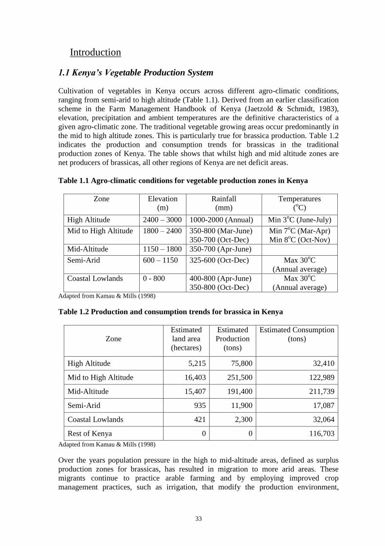
33

Introduction

1.1 Kenya’s Vegetable Production System

Cultivation of vegetables in Kenya occurs across different agro-climatic conditions,

ranging from semi-arid to high altitude (Table 1.1). Derived from an earlier classification

scheme in the Farm Management Handbook of Kenya (Jaetzold & Schmidt, 1983),

elevation, precipitation and ambient temperatures are the definitive characteristics of a

given agro-climatic zone. The traditional vegetable growing areas occur predominantly in

the mid to high altitude zones. This is particularly true for brassica production. Table 1.2

indicates the production and consumption trends for brassicas in the traditional

production zones of Kenya. The table shows that whilst high and mid altitude zones are

net producers of brassicas, all other regions of Kenya are net deficit areas.

Table 1.1 Agro-climatic conditions for vegetable production zones in Kenya

Zone Elevation

(m)

Rainfall

(mm)

Temperatures

(oC)

High Altitude 2400 – 3000 1000-2000 (Annual) Min 3oC (June-July)

Mid to High Altitude 1800 – 2400 350-800 (Mar-June)

350-700 (Oct-Dec)

Min 7oC (Mar-Apr)

Min 8oC (Oct-Nov)

Mid-Altitude 1150 – 1800 350-700 (Apr-June)

Semi-Arid 600 – 1150 325-600 (Oct-Dec) Max 30oC

(Annual average)

Coastal Lowlands 0 - 800 400-800 (Apr-June)

350-800 (Oct-Dec)

Max 30oC

(Annual average) Adapted from Kamau & Mills (1998)

Table 1.2 Production and consumption trends for brassica in Kenya

Zone

Estimated

land area

(hectares)

Estimated

Production

(tons)

Estimated Consumption

(tons)

High Altitude 5,215 75,800 32,410

Mid to High Altitude 16,403 251,500 122,989

Mid-Altitude 15,407 191,400 211,739

Semi-Arid 935 11,900 17,087

Coastal Lowlands 421 2,300 32,064

Rest of Kenya 0 0 116,703

Adapted from Kamau & Mills (1998)

Over the years population pressure in the high to mid-altitude areas, defined as surplus

production zones for brassicas, has resulted in migration to more arid areas. These

migrants continue to practice arable farming and by employing improved crop

management practices, such as irrigation, that modify the production environment,

34

vegetable production has expanded to the semi-arid zones. Rural to urban migration has

also resulted in a rapid growth of urban areas in Kenya, particularly Nairobi. The

resulting high population density and an ever-increasing demand for food has caused a

change in land-use systems in peri-urban areas of Nairobi. The area to the North and

North-West of Nairobi was traditionally a coffee growing zone. This zone currently

comprises upper market residential areas, smallholder vegetable farms and medium scale

flower farms. Likewise, previously large-scale ranches to the east of Nairobi have now

been subdivided into smallholder farms with plots close to Athi River producing

vegetables both for the export and local markets through irrigation.

1.2 The peri-urban production system

Peri-urban area by definition would be a region in the environs of an urban centre.

Although much debate still goes on about the definition of the peri-urban system,

especially the geographic scope, the recent focus is on functional attributes. According to

the United Nations Food and Agricultural Organisation “Urban and peri Urban

Agriculture is perceived as agriculture practices within and around cities which compete

for resources (land, water, energy, labour) that could also serve other purposes to satisfy

the requirements of the urban population” (FAO 1999).

Likewise, according to the Department for International Development of the United

Kingdom (DFID), Natural Resource Systems Programme, the peri-urban interface is

created by urban development. “Rural activities pre-exist. As urban activities proliferate

and grow, linkages relating to them are built from either the town or the countryside.

These cause changes to existing production systems and create new ones that can affect

the poor in urban and rural areas. Opportunities arise relating to easy access to markets

and services, with ready supplies of labour. Problems arise from shortage of land and

risks from pollution and continued urban growth”( http://www.nrinternational.co.uk/).

A study commissioned by DIFD, Crop Protection Programme (CPP), on factors affecting

uptake and adoption of outputs of crop protection research in peri-urban vegetable

systems in Kenya (Project R7512, ZA0357) identified the peri-urban vegetable

production system as an area in the immediate environs of an urban boundary where the

land use pattern, particularly vegetable production is influenced by the presence of a

given urban centre. In addition to a possible comparative advantage in vegetable

production arising from proximity to a market outlet, the peri-urban vegetable producers

target the dry season for production of most commodities. During the dry season, the

vegetable markets in urban centres are essentially a sellers‟ market, with demand

outstripping supply. The study also identified as peri-urban vegetable producing areas

surrounding Nairobi the administrative districts of; Kiambu, Machakos, Thika and

Kajiado (Otieno Oruko et al, 2000). Agro-climatically, these areas fall in the High to

Midland zones (Jaetzold & Schmidt, 1983 a & b).

Noteworthy about the above definitions are the competing opportunities for resources

especially land and labour, the primary factors of production in smallholder agriculture in

developing countries. In addition, easier access to input services and output markets

arising from proximity to urban centres and high opportunity cost of land and labour

provide a recipe for the development of a commercially oriented smallholder agricultural

production system.

http://www.nrinternational.co.uk/

35

1.3 The CPP Peri-urban cluster of projects

The Department for International Development (DFID) Crop Protection Programme

(CPP) Purpose of the Peri-urban Production System is to improve the volume, quality and

seasonal availability of food and crop products through the reduction of physical and

economic losses caused by pests. Previous studies (Oduor et al, 1998) identified pests and

diseases as the major production constraint. In addition, where chemicals are used to

control pests, there is widespread misuse causing environmental damage, promoting the

development of pesticide resistance in the pests and causing health problems (Cooper

1999). In order to address this situation (CPP) supports a thematic cluster of research

projects in the peri-urban vegetable systems in Kenya. The projects aim to develop

improved chemical and non-chemical control methods. In the peri-urban vegetable

systems in Kenya, these projects include the following.

Integrated management of root-knot nematodes on vegetables in Kenya (R7472,

1999-2002)

Pest management in horticultural crops; an integrated approach to vegetable pest

management with the aim of reducing reliance on pesticides in Kenya (ZA0082/3,

1996 – 1999; 1999-02)

Development of biorational brassica IPM in Kenya (A0869X1, 1999-2002)

Management of viruses and important vegetable crops in Kenya (ZA0376/R7571,

2000-2003)

A Participatory Rural Appraisal (PRA) undertaken in 1996 indicated that four main crops

(kale, cabbage, tomato and spinach) accounted for over 95% of peri-urban vegetable

production. Thus, these crops became the major focus of subsequent research activities.

Subsequent on-farm surveys to determine the incidence of pests and diseases in different

agro-ecological zones led to the prioritisation of the major pest and disease problems and

identification of areas of pest management which required improvement. Diamond Back

Moth (DBM), aphids and semi looper were found to be important pests of brassicas while

on spinach and tomatoes, leaf miner, aphids, semi looper and thrips were more important.

Diseases were not found to be particularly important on brassicas, the most damaging

being black rot, ring spot, downy mildew and virus. In contrast, diseases were found to

be extremely damaging on spinach and tomato including early blight, late blight, virus

and leaf spot. Also, the diversity and severity of pests were higher in the lower, warmer

locations i.e. Athi River, whereas in higher, cooler locations i.e. Nyathuna, the incidence

and severity of diseases was greater.

1.4 Objectives of the present survey

A socio-economic survey was commissioned as part of the Peri-Urban Production System

Cluster of Projects, to establish farmer practices and key characteristics of peri-urban

farms. The survey was designed with the following objectives:

To characterise peri-urban vegetable systems

To determine the main constraints to vegetable production in peri-urban areas

To determine farmer problems, perceptions and practices in relation to vegetable

pests and diseases, with particular reference to the Diamondback moth, root-knot

nematodes, aphids, blight and virus disease.

To establish coping strategies for pests and diseases and implications for the peri-

urban cluster of projects.

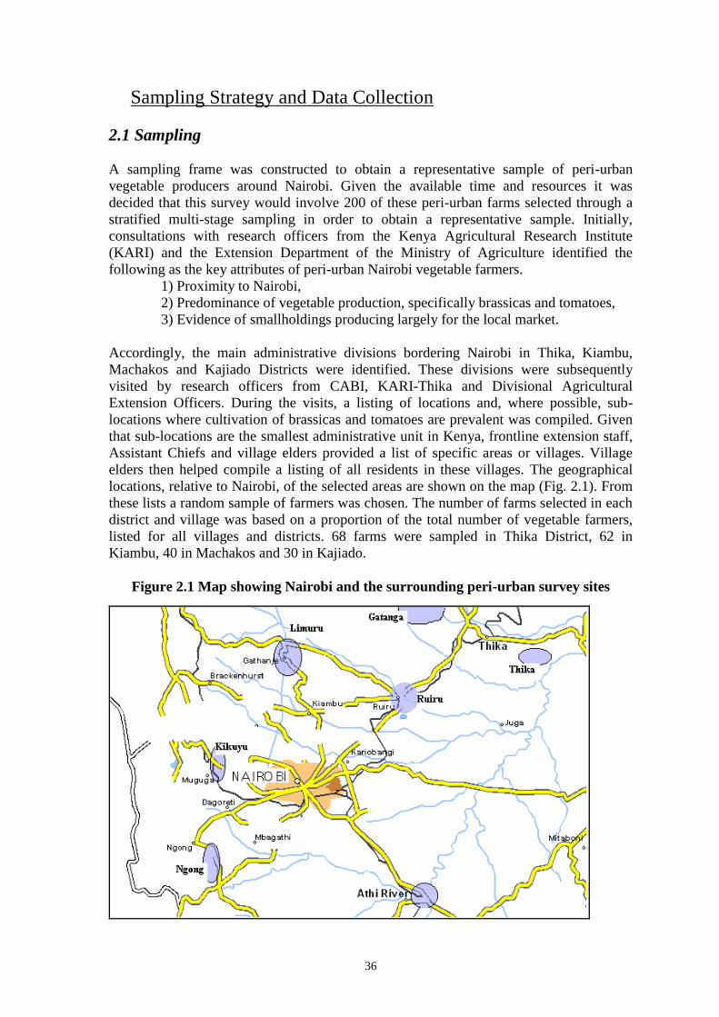
36

Sampling Strategy and Data Collection

2.1 Sampling

A sampling frame was constructed to obtain a representative sample of peri-urban

vegetable producers around Nairobi. Given the available time and resources it was

decided that this survey would involve 200 of these peri-urban farms selected through a

stratified multi-stage sampling in order to obtain a representative sample. Initially,

consultations with research officers from the Kenya Agricultural Research Institute

(KARI) and the Extension Department of the Ministry of Agriculture identified the

following as the key attributes of peri-urban Nairobi vegetable farmers.

1) Proximity to Nairobi,

2) Predominance of vegetable production, specifically brassicas and tomatoes,

3) Evidence of smallholdings producing largely for the local market.

Accordingly, the main administrative divisions bordering Nairobi in Thika, Kiambu,

Machakos and Kajiado Districts were identified. These divisions were subsequently

visited by research officers from CABI, KARI-Thika and Divisional Agricultural

Extension Officers. During the visits, a listing of locations and, where possible, sub-

locations where cultivation of brassicas and tomatoes are prevalent was compiled. Given

that sub-locations are the smallest administrative unit in Kenya, frontline extension staff,

Assistant Chiefs and village elders provided a list of specific areas or villages. Village

elders then helped compile a listing of all residents in these villages. The geographical

locations, relative to Nairobi, of the selected areas are shown on the map (Fig. 2.1). From

these lists a random sample of farmers was chosen. The number of farms selected in each

district and village was based on a proportion of the total number of vegetable farmers,

listed for all villages and districts. 68 farms were sampled in Thika District, 62 in

Kiambu, 40 in Machakos and 30 in Kajiado.

Figure 2.1 Map showing Nairobi and the surrounding peri-urban survey sites

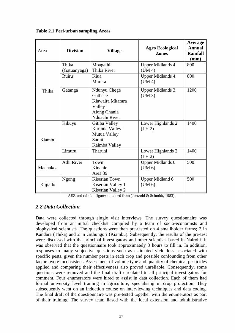
37

Table 2.1 Peri-urban sampling Areas

Area Division Village Agro Ecological

Zones

Average

Annual

Rainfall

(mm)

Thika

Thika

(Gatuanyaga)

Mbagathi

Thika River

Upper Midlands 4

(UM 4)

800

Ruiru Kiua

Murera

Upper Midlands 4

(UM 4)

800

Gatanga Ndunyu Chege

Gathece

Kiawaira Mkarara

Valley

Along Chania

Nduachi River

Upper Midlands 3

(UM 3)

1200

Kiambu

Kikuyu Gitiba Valley

Karinde Valley

Mutua Valley

Samiti

Kaimba Valley

Lower Highlands 2

(LH 2)

1400

Limuru Tharuni Lower Highlands 2

(LH 2)

1400

Machakos

Athi River Town

Kinanie

Area 39

Upper Midlands 6

(UM 6)

500

Kajiado

Ngong Kiserian Town

Kiserian Valley 1

Kiserian Valley 2

Upper Midland 6

(UM 6)

500

AEZ and rainfall figures obtained from (Jaetzold & Schmidt, 1983)

2.2 Data Collection

Data were collected through single visit interviews. The survey questionnaire was

developed from an initial checklist compiled by a team of socio-economists and

biophysical scientists. The questions were then pre-tested on 4 smallholder farms; 2 in

Kandara (Thika) and 2 in Githunguri (Kiambu). Subsequently, the results of the pre-test

were discussed with the principal investigators and other scientists based in Nairobi. It

was observed that the questionnaire took approximately 3 hours to fill in. In addition,

responses to many subjective questions such as estimated yield loss associated with

specific pests, given the number pests in each crop and possible confounding from other

factors were inconsistent. Assessment of volume type and quantity of chemical pesticides

applied and comparing their effectiveness also proved unreliable. Consequently, some

questions were removed and the final draft circulated to all principal investigators for

comment. Four enumerators were hired to assist in data collection. Each of them had

formal university level training in agriculture, specialising in crop protection. They

subsequently went on an induction course on interviewing techniques and data coding.

The final draft of the questionnaire was pre-tested together with the enumerators as part

of their training. The survey team liased with the local extension and administrative

38

officials in each division to identify the sample farms and inform them about the

interviews in advance. All the interviews were conducted on the farms, in the absence of

local extension officials who might have influenced the responses. It was established,

during the pre-test, that each interview would take between one and one and a half hours.

Each enumerator was therefore assigned three farms per day, in order to enhance

accuracy and avoid fatigue. The survey was conducted over a period of one month from

July 15th

to August 15th

2000. Data was analysed using Statistical Package for Social

Sciences (SPSS) Version 7.5, GENSTAT 5 and Microsoft Excel 2000.

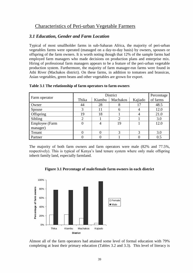
39

Characteristics of Peri-urban Vegetable Farmers

3.1 Education, Gender and Farm Location

Typical of most smallholder farms in sub-Saharan Africa, the majority of peri-urban

vegetables farms were operated (managed on a day-to-day basis) by owners, spouses or

offspring of the farm owners. It is worth noting though that 12% of the sample farms had

employed farm managers who made decisions on production plans and enterprise mix.

Hiring of professional farm managers appears to be a feature of the peri-urban vegetable

production system. Furthermore, the majority of farm manager-run farms were found in

Athi River (Machakos district). On these farms, in addition to tomatoes and brassicas,

Asian vegetables, green beans and other vegetables are grown for export.

Table 3.1 The relationship of farm operators to farm owners

Farm operator District Percentage

Thika Kiambu Machakos Kajiado of farms

Owner 44 28 8 17 48.5

Spouse 3 11 6 4 12.0

Offspring 19 18 1 4 21.0

Sibling 2 1 2 1 3.0

Employee (Farm

manager)

0 4 19 1 12.0

Tenant 0 0 3 3 3.0

Partner 0 0 1 0 0.5

The majority of both farm owners and farm operators were male (82% and 77.5%,

respectively). This is typical of Kenya‟s land tenure system where only male offspring

inherit family land, especially farmland.

Figure 3.1 Percentage of male/female farm owners in each district

0%

20%

40%

60%

80%

100%

Thika Kiambu Machakos Kajiado

District

Perc

en

tage

of

farm

ow

ners

Female

Male

Almost all of the farm operators had attained some level of formal education with 79%

completing at least their primary education (Tables 3.2 and 3.3). This level of literacy is

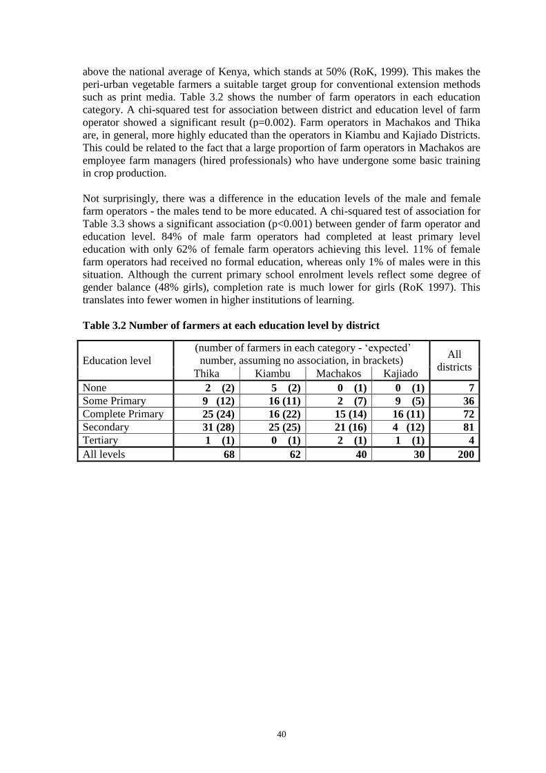
40

above the national average of Kenya, which stands at 50% (RoK, 1999). This makes the

peri-urban vegetable farmers a suitable target group for conventional extension methods

such as print media. Table 3.2 shows the number of farm operators in each education

category. A chi-squared test for association between district and education level of farm

operator showed a significant result (p=0.002). Farm operators in Machakos and Thika

are, in general, more highly educated than the operators in Kiambu and Kajiado Districts.

This could be related to the fact that a large proportion of farm operators in Machakos are

employee farm managers (hired professionals) who have undergone some basic training

in crop production.

Not surprisingly, there was a difference in the education levels of the male and female

farm operators - the males tend to be more educated. A chi-squared test of association for

Table 3.3 shows a significant association (p<0.001) between gender of farm operator and

education level. 84% of male farm operators had completed at least primary level

education with only 62% of female farm operators achieving this level. 11% of female

farm operators had received no formal education, whereas only 1% of males were in this

situation. Although the current primary school enrolment levels reflect some degree of

gender balance (48% girls), completion rate is much lower for girls (RoK 1997). This

translates into fewer women in higher institutions of learning.

Table 3.2 Number of farmers at each education level by district

Education level

(number of farmers in each category - „expected‟

number, assuming no association, in brackets) All

districts Thika Kiambu Machakos Kajiado

None 2 (2) 5 (2) 0 (1) 0 (1) 7

Some Primary 9 (12) 16 (11) 2 (7) 9 (5) 36

Complete Primary 25 (24) 16 (22) 15 (14) 16 (11) 72

Secondary 31 (28) 25 (25) 21 (16) 4 (12) 81

Tertiary 1 (1) 0 (1) 2 (1) 1 (1) 4

All levels 68 62 40 30 200

41

Table 3.3 Education level and gender of farm operators

Education level of farm operator

(percentages, by gender, in brackets) Total

Gender

None Some

Primary

Complete

Primary

Secondary Tertiary

Female 5 (11.1) 12 (26.7) 20 (44.4) 8 (17.8) 0 (0) 45

Male 2 (1.3) 24 (15.5) 52 (33.5) 73 (47.1) 4 (2.6) 155

Total 7 (3.5) 36 (18.0) 72 (36.0) 81 (40.5) 4 (2.0) 200

The average age for farm operators was 38, and for farm owners it was 49 years old. Ages

of both farm owners and farm operators ranged from 20 to 90 years old. 27% of farm

operators were below the age of 30, but by contrast, only 9% of farm owners were below

this age. Table 3.4 shows that the higher educated farm operators and owners were, on

average, younger than their less educated neighbours.

Table 3.4 Age of farm owners and farm operators in each education category

Average age (standard deviations in brackets)

Education level Farm owner Farm operator

None 54 (9) 54 (9)

Some Primary 52 (18) 45 (17)

Complete Primary 47 (17) 35 (10)

Secondary 49 (15) 35 (9)

Tertiary 37 (10) 32 (6)

All levels 49 (16) 38 (12)

In order to gain insights into the relative wealth status of the farmers, farmers were asked

questions concerning ownership of cattle, motor-vehicle and water tank (Table 3.5).

Water tank and cattle ownership is particularly high in Kiambu district while Machakos

district has the highest proportion of farmers owning a vehicle.

Table 3.5 Ownership of water tank, cattle and motor vehicle by district

(percentage within district in brackets)

District Water Tank Cattle Vehicle

Thika 14 (21) 44 (65) 4 (6)

Kiambu 41 (66) 52 (84) 13 (21)

Machakos 15 (38) 16 (40) 16 (40)

Kajiado 10 (33) 10 (33) 5 (17)

All Districts 80 (40) 122 (61) 38 (19)

On average, farmers in Thika district lived the furthest from an all-weather road. They

also had the greatest distance to travel to market, 14.4 km on average.

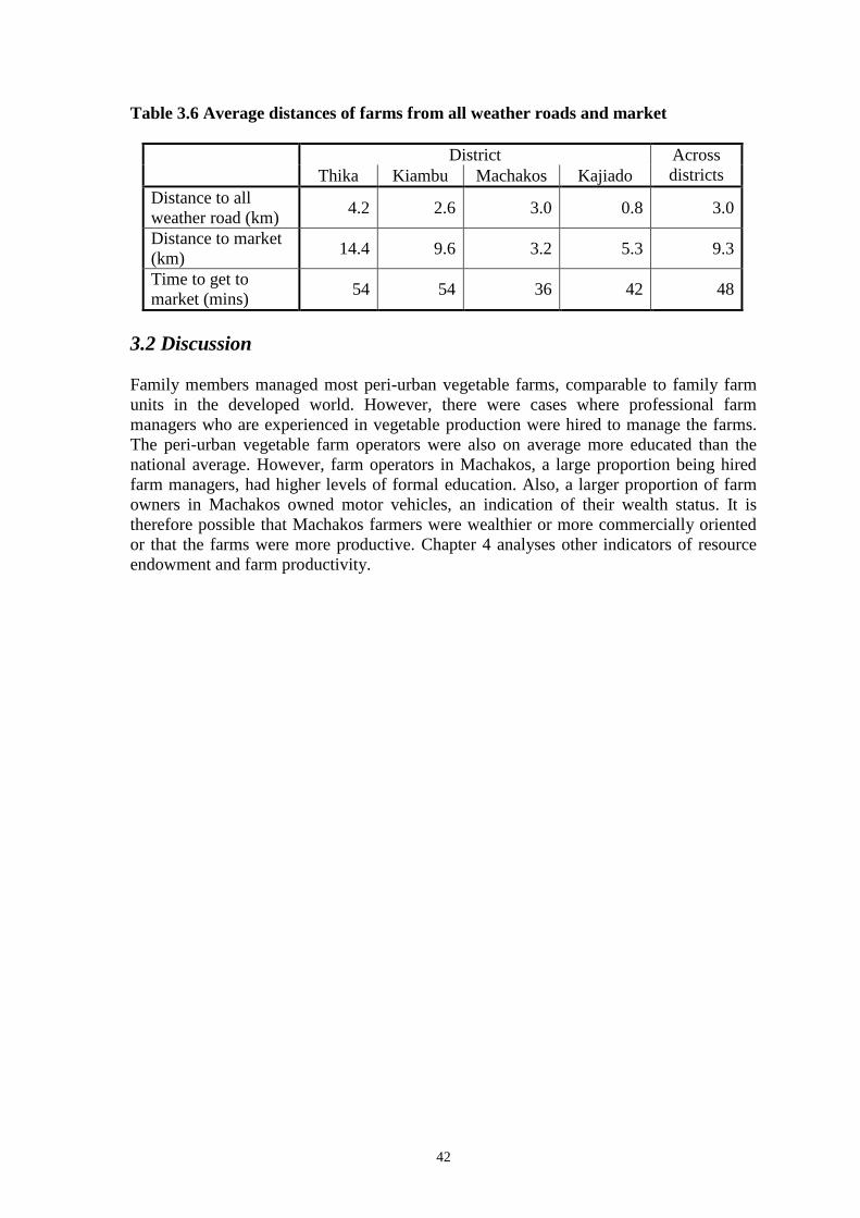
42

Table 3.6 Average distances of farms from all weather roads and market

District Across

districts Thika Kiambu Machakos Kajiado

Distance to all

weather road (km) 4.2 2.6 3.0 0.8 3.0

Distance to market

(km) 14.4 9.6 3.2 5.3 9.3

Time to get to

market (mins) 54 54 36 42 48

3.2 Discussion

Family members managed most peri-urban vegetable farms, comparable to family farm

units in the developed world. However, there were cases where professional farm

managers who are experienced in vegetable production were hired to manage the farms.

The peri-urban vegetable farm operators were also on average more educated than the

national average. However, farm operators in Machakos, a large proportion being hired

farm managers, had higher levels of formal education. Also, a larger proportion of farm

owners in Machakos owned motor vehicles, an indication of their wealth status. It is

therefore possible that Machakos farmers were wealthier or more commercially oriented

or that the farms were more productive. Chapter 4 analyses other indicators of resource

endowment and farm productivity.

43

Vegetable Production and Marketing Systems

4.1 Cropping System - Land area under vegetables

It was hypothesised in Chapter 1 that smallholder farms typify the peri-urban vegetable

production system. Table 4.1 shows that the average farm size was 1.3 hectares, with a

cropped area of 0.8 hectares. Farms in Machakos district were, on average, larger than the

other survey districts. In all districts except Thika, vegetable area constituted over 50% of

the cropped area at the time of the survey. This proportion is highest in Kajiado district

where 85% of the cropped land on a farm was given over to vegetable production. The

percentage of Kajiado farmers renting land for vegetable production (53%) is also higher

than the other districts (23-26%).

Table 4.1 Average farm size, cropped and vegetable areas (in hectares)

District All

districts (average areas in hectares) Thika Kiambu Machakos Kajiado

Vegetable area of farm 0.3 (0.3) 0.4 (0.4) 0.7 (0.6) 0.4 (0.3) 0.4 (0.4)

Cropped area of farm 0.8 (0.8) 0.7 (0.6) 1.1 (1.1) 0.5 (0.4) 0.8 (0.8)

Total farm size 1.1 (1.0) 1.2 (1.1) 2.3 (2.1) 0.8 (0.6) 1.3 (1.4)

Vegetable area as percentage

of cropped farm area 39% 59% 65% 85% 55%

Vegetable area as percentage

of total farm 28% 35% 32% 50% 33%

Number of farmers renting

land for vegetable crop

17

(25%)

16

(26%)

9

(23%)

16

(53%)

58

(29%) (standard deviations in brackets for first three rows)

Table 4.3 and Figure 4.1 give a breakdown of vegetable area into the three vegetables,

tomatoes, kale and cabbage. The average size of vegetable area is also shown as a

proportion of the cropped area within a farm.

Table 4.2 Number of farmers growing vegetables in each district

District

Thika Kiambu Machakos Kajiado All districts

Tomato 59 (87) 24 (39) 34 (85) 25 (83) 142 (71)

Kale 54 (79) 46 (74) 34 (85) 25 (83) 159 (80)

Cabbage 5 (7) 43 (69) 32 (80) 18 (60) 98 (49) (Percentage of farmers in brackets)

44

Table 4.3 Average cropped area by district (hectares)

District All

districts (average areas in hectares) Thika Kiambu Machakos Kajiado

Tomato crop land area 0.13

(0.13)

0.16

(0.10)

0.38

(0.36)

0.16

(0.16)

0.21

(0.24)

Proportion of cropped land

under tomatoes

0.19

(0.20)

0.25

(0.20)

0.35

(0.24)

0.39

(0.29)

0.27

(0.24)

Kale crop land area 0.08

(0.06)

0.12

(0.09)

0.26

(0.25)

0.11

(0.09)

0.13

(0.15)


under kale

0.17

(0.22)

0.27

(0.21)

0.26

(0.23)

0.26

(0.18)

0.23

(0.22)

Cabbage crop land area 0.13

(0.15)

0.23

(0.15)

0.29

(0.38)

0.16

(0.11)

0.20

(0.20)


under cabbage

0.27

(0.68)

0.32

(0.24)

0.17

(0.19)

0.37

(0.29)

0.29

(0.45) (standard deviations in brackets)

Figure 4.1 Average vegetable crop size (hectares) and proportion of cropped area of

farm under each vegetable.

4.2. Varietal adoption and seed sources

The predominant tomato variety grown is Cal J. This variety produces hard fruit and has

good storage quality (long shelf life) compared with the Moneymaker variety. Cal J is

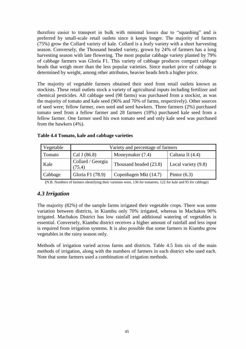
45

therefore easier to transport in bulk with minimal losses due to “squashing” and is

preferred by small-scale retail outlets since it keeps longer. The majority of farmers

(75%) grow the Collard variety of kale. Collard is a leafy variety with a short harvesting

season. Conversely, the Thousand headed variety, grown by 24% of farmers has a long

harvesting season with late flowering. The most popular cabbage variety planted by 79%

of cabbage farmers was Gloria F1. This variety of cabbage produces compact cabbage

heads that weigh more than the less popular varieties. Since market price of cabbage is

determined by weight, among other attributes, heavier heads fetch a higher price.

The majority of vegetable farmers obtained their seed from retail outlets known as

stockists. These retail outlets stock a variety of agricultural inputs including fertilizer and

chemical pesticides. All cabbage seed (98 farms) was purchased from a stockist, as was

the majority of tomato and kale seed (96% and 70% of farms, respectively). Other sources

of seed were; fellow farmer, own seed and seed hawkers. Three farmers (2%) purchased

tomato seed from a fellow farmer and 28 farmers (18%) purchased kale seed from a

fellow farmer. One farmer used his own tomato seed and only kale seed was purchased

from the hawkers (4%).

Table 4.4 Tomato, kale and cabbage varieties

Vegetable Variety and percentage of farmers

Tomato Cal J (86.8) Moneymaker (7.4) Caltana II (4.4)

Kale Collard / Georgia

(75.4) Thousand headed (23.8) Local variety (9.8)

Cabbage Gloria F1 (78.9) Copenhagen Mkt (14.7) Pintor (6.3)

(N.B. Numbers of farmers identifying their varieties were, 136 for tomatoes, 122 for kale and 95 for cabbage)

4.3 Irrigation

The majority (82%) of the sample farms irrigated their vegetable crops. There was some

variation between districts, in Kiambu only 70% irrigated, whereas in Machakos 90%

irrigated. Machakos District has low rainfall and additional watering of vegetables is

essential. Conversely, Kiambu district receives a higher amount of rainfall and less input

is required from irrigation systems. It is also possible that some farmers in Kiambu grow

vegetables in the rainy season only.

Methods of irrigation varied across farms and districts. Table 4.5 lists six of the main

methods of irrigation, along with the numbers of farmers in each district who used each.

Note that some farmers used a combination of irrigation methods.

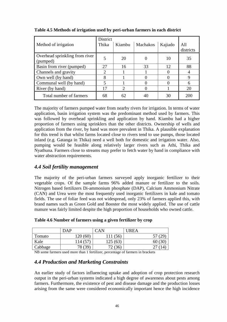
46

Table 4.5 Methods of irrigation used by peri-urban farmers in each district

Method of irrigation

District

Thika Kiambu Machakos Kajiado All

districts

Overhead sprinkling from river

(pumped) 5 20 0 10 35

Basin from river (pumped) 27 16 33 12 88

Channels and gravity 2 1 1 0 4

Own well (by hand) 8 1 0 0 9

Communal well (by hand) 5 1 0 0 6

River (by hand) 17 2 0 1 20

Total number of farmers 68 62 40 30 200

The majority of farmers pumped water from nearby rivers for irrigation. In terms of water

application, basin irrigation system was the predominant method used by farmers. This

was followed by overhead sprinkling and application by hand. Kiambu had a higher

proportion of farmers using sprinklers than the other districts. Ownership of wells and

application from the river, by hand was more prevalent in Thika. A plausible explanation

for this trend is that whilst farms located close to rivers tend to use pumps, those located

inland (e.g. Gatanga in Thika) need a well both for domestic and irrigation water. Also,

pumping would be feasible along relatively larger rivers such as Athi, Thika and

Nyathuna. Farmers close to streams may prefer to fetch water by hand in compliance with

water abstraction requirements.

4.4 Soil fertility management

The majority of the peri-urban farmers surveyed apply inorganic fertilizer to their

vegetable crops. Of the sample farms 96% added manure or fertilizer to the soils.

Nitrogen based fertilizers Di-ammonium phosphate (DAP), Calcium Ammonium Nitrate

(CAN) and Urea were the most frequently used inorganic fertilizers in kale and tomato

fields. The use of foliar feed was not widespread, only 23% of farmers applied this, with

brand names such as Green Gold and Booster the most widely applied. The use of cattle

manure was fairly limited despite the high proportion of households who owned cattle.

Table 4.6 Number of farmers using a given fertilizer by crop

DAP CAN UREA

Tomato 120 (60) 111 (56) 57 (29)

Kale 114 (57) 125 (63) 60 (30)

Cabbage 78 (39) 72 (36) 27 (14) NB some farmers used more than 1 fertilizer, percentage of farmers in brackets

4.4 Production and Marketing Constraints

An earlier study of factors influencing uptake and adoption of crop protection research

output in the peri-urban systems indicated a high degree of awareness about pests among

farmers. Furthermore, the existence of pest and disease damage and the production losses

arising from the same were considered economically important hence the high incidence

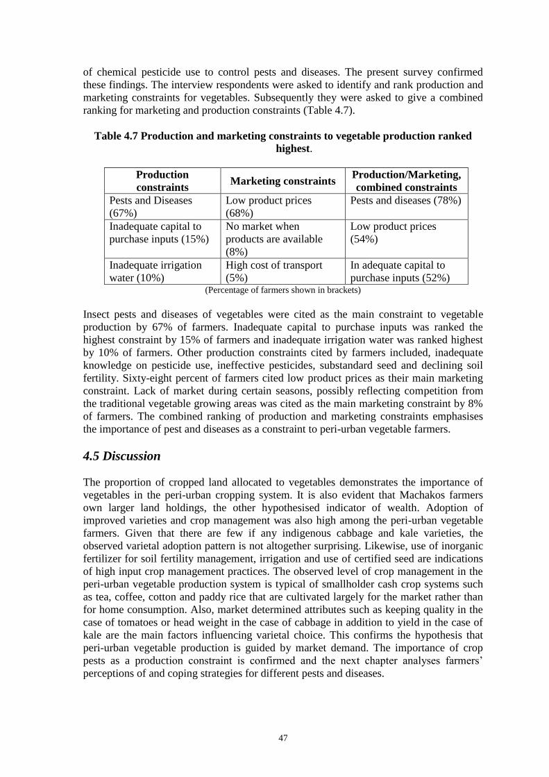
47

of chemical pesticide use to control pests and diseases. The present survey confirmed

these findings. The interview respondents were asked to identify and rank production and

marketing constraints for vegetables. Subsequently they were asked to give a combined

ranking for marketing and production constraints (Table 4.7).

Table 4.7 Production and marketing constraints to vegetable production ranked

highest.

Production

constraints Marketing constraints

Production/Marketing,

combined constraints

Pests and Diseases

(67%)

Low product prices

(68%)

Pests and diseases (78%)

Inadequate capital to

purchase inputs (15%)

No market when

products are available

(8%)

Low product prices

(54%)

Inadequate irrigation

water (10%)

High cost of transport

(5%)

In adequate capital to

purchase inputs (52%) (Percentage of farmers shown in brackets)

Insect pests and diseases of vegetables were cited as the main constraint to vegetable

production by 67% of farmers. Inadequate capital to purchase inputs was ranked the

highest constraint by 15% of farmers and inadequate irrigation water was ranked highest

by 10% of farmers. Other production constraints cited by farmers included, inadequate

knowledge on pesticide use, ineffective pesticides, substandard seed and declining soil

fertility. Sixty-eight percent of farmers cited low product prices as their main marketing

constraint. Lack of market during certain seasons, possibly reflecting competition from

the traditional vegetable growing areas was cited as the main marketing constraint by 8%

of farmers. The combined ranking of production and marketing constraints emphasises

the importance of pest and diseases as a constraint to peri-urban vegetable farmers.

4.5 Discussion

The proportion of cropped land allocated to vegetables demonstrates the importance of

vegetables in the peri-urban cropping system. It is also evident that Machakos farmers

own larger land holdings, the other hypothesised indicator of wealth. Adoption of

improved varieties and crop management was also high among the peri-urban vegetable

farmers. Given that there are few if any indigenous cabbage and kale varieties, the

observed varietal adoption pattern is not altogether surprising. Likewise, use of inorganic

fertilizer for soil fertility management, irrigation and use of certified seed are indications

of high input crop management practices. The observed level of crop management in the

peri-urban vegetable production system is typical of smallholder cash crop systems such

as tea, coffee, cotton and paddy rice that are cultivated largely for the market rather than

for home consumption. Also, market determined attributes such as keeping quality in the

case of tomatoes or head weight in the case of cabbage in addition to yield in the case of

kale are the main factors influencing varietal choice. This confirms the hypothesis that

peri-urban vegetable production is guided by market demand. The importance of crop

pests as a production constraint is confirmed and the next chapter analyses farmers‟

perceptions of and coping strategies for different pests and diseases.

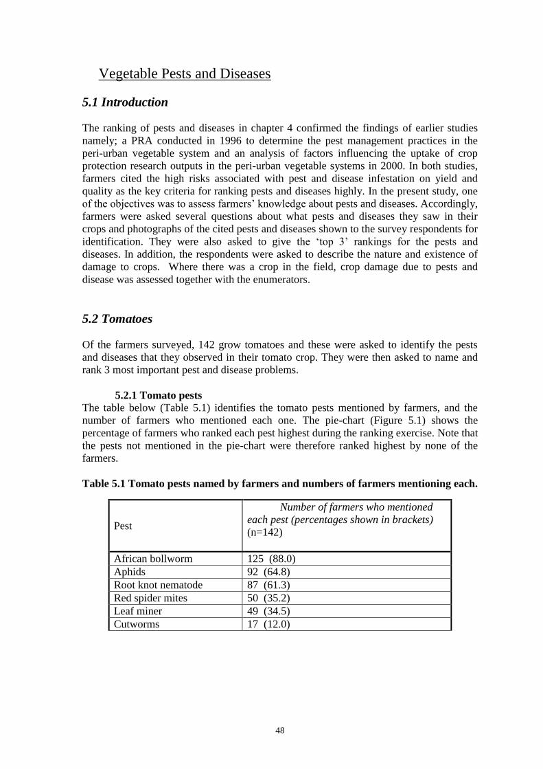
48

Vegetable Pests and Diseases

5.1 Introduction

The ranking of pests and diseases in chapter 4 confirmed the findings of earlier studies

namely; a PRA conducted in 1996 to determine the pest management practices in the

peri-urban vegetable system and an analysis of factors influencing the uptake of crop

protection research outputs in the peri-urban vegetable systems in 2000. In both studies,

farmers cited the high risks associated with pest and disease infestation on yield and

quality as the key criteria for ranking pests and diseases highly. In the present study, one

of the objectives was to assess farmers‟ knowledge about pests and diseases. Accordingly,

farmers were asked several questions about what pests and diseases they saw in their

crops and photographs of the cited pests and diseases shown to the survey respondents for

identification. They were also asked to give the „top 3‟ rankings for the pests and

diseases. In addition, the respondents were asked to describe the nature and existence of

damage to crops. Where there was a crop in the field, crop damage due to pests and

disease was assessed together with the enumerators.

5.2 Tomatoes

Of the farmers surveyed, 142 grow tomatoes and these were asked to identify the pests

and diseases that they observed in their tomato crop. They were then asked to name and

rank 3 most important pest and disease problems.

5.2.1 Tomato pests

The table below (Table 5.1) identifies the tomato pests mentioned by farmers, and the

number of farmers who mentioned each one. The pie-chart (Figure 5.1) shows the

percentage of farmers who ranked each pest highest during the ranking exercise. Note that

the pests not mentioned in the pie-chart were therefore ranked highest by none of the

farmers.

Table 5.1 Tomato pests named by farmers and numbers of farmers mentioning each.

Pest

Number of farmers who mentioned

each pest (percentages shown in brackets)

(n=142)

African bollworm 125 (88.0)

Aphids 92 (64.8)

Root knot nematode 87 (61.3)

Red spider mites 50 (35.2)

Leaf miner 49 (34.5)

Cutworms 17 (12.0)

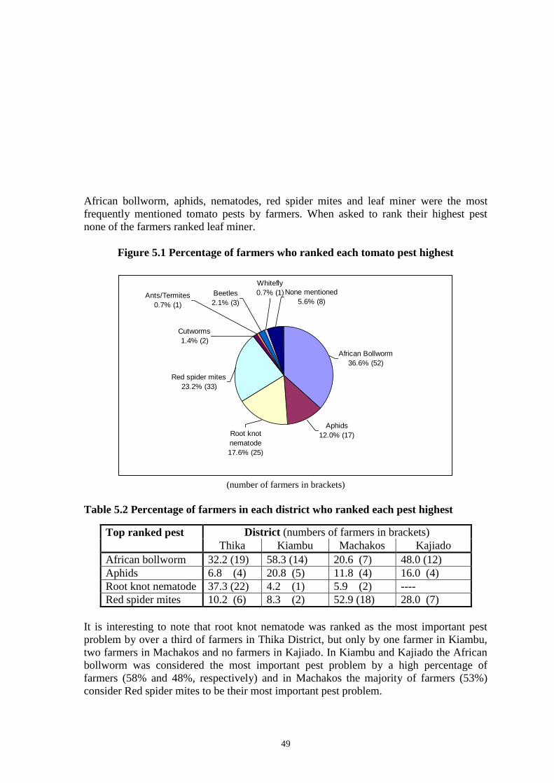
49

African bollworm, aphids, nematodes, red spider mites and leaf miner were the most

frequently mentioned tomato pests by farmers. When asked to rank their highest pest

none of the farmers ranked leaf miner.

Figure 5.1 Percentage of farmers who ranked each tomato pest highest

Root knot

nematode

17.6% (25)

Red spider mites

23.2% (33)

Aphids

12.0% (17)

African Bollworm

36.6% (52)

None mentioned

5.6% (8)Ants/Termites

0.7% (1)

Whitefly

0.7% (1)

Cutworms

1.4% (2)

Beetles

2.1% (3)

(number of farmers in brackets)

Table 5.2 Percentage of farmers in each district who ranked each pest highest

Top ranked pest District (numbers of farmers in brackets)

Thika Kiambu Machakos Kajiado

African bollworm 32.2 (19) 58.3 (14) 20.6 (7) 48.0 (12)

Aphids 6.8 (4) 20.8 (5) 11.8 (4) 16.0 (4)

Root knot nematode 37.3 (22) 4.2 (1) 5.9 (2) ----

Red spider mites 10.2 (6) 8.3 (2) 52.9 (18) 28.0 (7)

It is interesting to note that root knot nematode was ranked as the most important pest

problem by over a third of farmers in Thika District, but only by one farmer in Kiambu,

two farmers in Machakos and no farmers in Kajiado. In Kiambu and Kajiado the African

bollworm was considered the most important pest problem by a high percentage of

farmers (58% and 48%, respectively) and in Machakos the majority of farmers (53%)

consider Red spider mites to be their most important pest problem.

50

Table 5.3 Percentage of farmers who ranked each pest highest – shown for irrigated

farms and non-irrigated farms

Top ranked pest Irrigation treatment (numbers of farmers in brackets)

Non-irrigated Irrigated

African bollworm 31.8 (7) 37.5 (45)

Aphids 27.3 (6) 9.2 (11)

Root knot nematode 9.1 (2) 19.2 (23)

Red spider mites 22.7 (5) 23.3 (28)

Cut worms ---- 1.7 (2)

Ants/termites ---- 0.8 (1)

Beetles 4.5 (1) 1.7 (2)

Whitefly ---- 0.8 (1)

None mentioned 4.5 (1) 5.8 (7)

27% of farmers who do not irrigate, rank aphids as their most important pest problem,

compared to only 9% of farmers who do irrigate. Conversely only 9% of farmers who do

not irrigate rank root knot nematode as their worst pest problem, compared to 19% of

farmers who do irrigate. Farmers who do not irrigate did not rank cutworms, ants and

termites or whitefly as their worse pest problem, although four farmers who do irrigate

gave highest ranking to these pests.

5.2.2 Control of tomato pests

Only 4 out of the 142 farmers growing tomatoes did not apply some form of pest control

to their crop. Farmers were asked to name the chemical, botanical, biological and cultural

practice controls that they used to control the three most frequently mentioned pests, the

African bollworm, aphids and root knot nematode. It was found that the numbers of

farmers using botanical, biological or cultural practice controls was very small (1-5

farmers for each pest). The table below (Table 5.4) shows the most frequently used

chemical control for the tomato pests.

Table 5.4 Chemicals used by farmers to control tomato insect pests

Pest

Chemicals most

frequently used for

control of pest

Number of tomato

growing farmers

using this control

(%)

Total number of

farmers using some

form of chemical

control (%)

African

Bollworm

Karate (Lambda –

cyhalothrin)

Dimethoate

(Dimethoate)

25 (17.6)

17 (12.0) 74 (52.1)

Aphids Karate (Lambda –

cyhalothrin)

Dimethoate(Dimethoate)

Diazinon (Diazinon)

59 (41.5)

31 (21.8)

21 (14.8) 107 (75.4)

Nematodes Furadan (Carbofuran) 16 (11.3) 28 (19.7)

5.2.3 Tomato diseases

The table below (Table 5.5) identifies the tomato diseases mentioned by farmers, and the


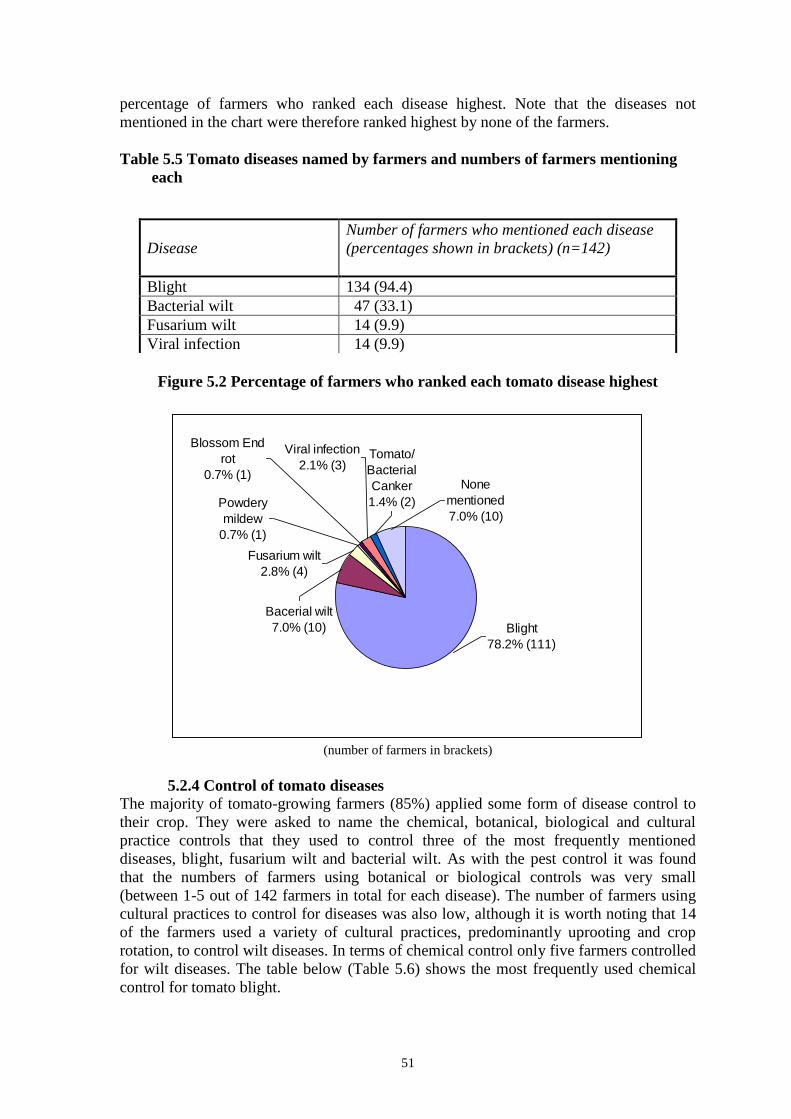
51

percentage of farmers who ranked each disease highest. Note that the diseases not

mentioned in the chart were therefore ranked highest by none of the farmers.

Table 5.5 Tomato diseases named by farmers and numbers of farmers mentioning

each

Figure 5.2 Percentage of farmers who ranked each tomato disease highest

Tomato/

Bacterial

Canker

1.4% (2)

Blossom End

rot

0.7% (1)None

mentioned

7.0% (10)

Viral infection

2.1% (3)

Blight

78.2% (111)

Bacerial wilt

7.0% (10)

Powdery

mildew

0.7% (1)

Fusarium wilt

2.8% (4)


5.2.4 Control of tomato diseases

The majority of tomato-growing farmers (85%) applied some form of disease control to

their crop. They were asked to name the chemical, botanical, biological and cultural

practice controls that they used to control three of the most frequently mentioned

diseases, blight, fusarium wilt and bacterial wilt. As with the pest control it was found

that the numbers of farmers using botanical or biological controls was very small

(between 1-5 out of 142 farmers in total for each disease). The number of farmers using

cultural practices to control for diseases was also low, although it is worth noting that 14

of the farmers used a variety of cultural practices, predominantly uprooting and crop

rotation, to control wilt diseases. In terms of chemical control only five farmers controlled

for wilt diseases. The table below (Table 5.6) shows the most frequently used chemical

control for tomato blight.

Disease

Number of farmers who mentioned each disease

(percentages shown in brackets) (n=142)

Blight 134 (94.4)

Bacterial wilt 47 (33.1)

Fusarium wilt 14 (9.9)

Viral infection 14 (9.9)

52

Table 5.6 Chemicals used by farmers to control tomato diseases

Disease Chemicals most

frequently used

for control of

disease

Number of tomato

growing farmers

using this control

(%)

Total number of farmers

using some form of

chemical control (%)

Blight Dithane M45

(Mancozeb)

Ridomil

(Metalaxyl)

73 (51.4)

60 (42.3) 122 (85.9)

5.3 Kale

Of the farmers surveyed, 159 grow kale and these farmers were asked to identify the pests

and diseases that they observed in their kale crop. They were then asked to rank their „top

3‟ most important pest and disease problems.

5.3.1 Kale pests

The table below (Table 5.7) identifies the kale pests mentioned by farmers, and the




farmers.

Table 5.7 Kale pests named by farmers and numbers of farmers mentioning each

Aphids, diamondback (DBM) moth and loopers were the most frequently mentioned

tomato pests by farmers. They were also the three pests that received the majority of

„highest‟ rankings from farmers.

Pest

Number of farmers who mentioned each pest


Aphids 155 (97.5)

Diamondback Moth 120 (75.5)

Loopers 106 (66.7)

Cutworms 19 (11.9)

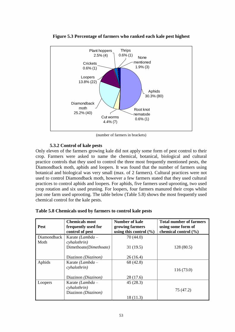
53

Figure 5.3 Percentage of farmers who ranked each kale pest highest

Plant hoppers

2.5% (4)

Loopers

13.8% (22)

Thrips

0.6% (1)

Crickets

0.6% (1)

None

mentioned

1.9% (3)

Aphids

30.3% (80)

Root knot

nematode

0.6% (1)

Diamondback

moth

25.2% (40)Cut worms

4.4% (7)


5.3.2 Control of kale pests

Only eleven of the farmers growing kale did not apply some form of pest control to their

crop. Farmers were asked to name the chemical, botanical, biological and cultural

practice controls that they used to control the three most frequently mentioned pests, the

Diamondback moth, aphids and loopers. It was found that the number of farmers using

botanical and biological was very small (max. of 2 farmers). Cultural practices were not

used to control Diamondback moth, however a few farmers stated that they used cultural

practices to control aphids and loopers. For aphids, five farmers used uprooting, two used

crop rotation and six used pruning. For loopers, four farmers manured their crops whilst

just one farm used uprooting. The table below (Table 5.8) shows the most frequently used

chemical control for the kale pests.

Table 5.8 Chemicals used by farmers to control kale pests

Pest

Chemicals most

frequently used for

control of pest

Number of kale

growing farmers

using this control (%)


using some form of


Diamondback

Moth

Karate (Lambda –

cyhalothrin)

Dimethoate(Dimethoate)

Diazinon (Diazinon)

70 (44.0)

31 (19.5)

26 (16.4)

128 (80.5)


cyhalothrin)

Diazinon (Diazinon)

68 (42.8)

28 (17.6)

116 (73.0)

Loopers Karate (Lambda –

cyhalothrin)

Diazinon (Diazinon)

45 (28.3)

18 (11.3)

75 (47.2)

54

5.3.3 Kale diseases

The table below (Table 5.9) identifies the kale diseases mentioned by farmers, and the


percentage of farmers who ranked each disease highest. Note that the diseases not

mentioned in the chart were therefore ranked highest by none of the farmers.

Table 5.9 Kale diseases named by farmers and numbers of farmers mentioning each

Figure 5.4 Percentage of farmers who ranked each kale disease highest

Powdery

mildew

3.8% (6)

Viral infection

34.0% (54)

Bacterial wilt

1.3% (2)

Blight

1.3% (2)

Blackleg

17.0% 27)

Blackrot

17.0% (27)

None

mentioned

24.5% (29)


5.1.4 Control of kale diseases

Only 31% of kale farmers said that they apply some form of disease control to their crop.

They were asked to name the chemical, botanical, biological and cultural practice controls

that they used to control four of the most frequently mentioned diseases, viral infection,

blackrot, blackleg and powdery mildew. It was found that no farmers were using

botanical or biological controls. The number of farmers using cultural practices to control

for diseases was also low, although it is worth noting that 17 of the farmers used a variety

of cultural practices, predominantly uprooting and crop rotation, to control for blackrot.

Also, 12 farmers stated that they were using these same cultural practices to control viral

infection. Eight farmers were using uprooting as a way of controlling for blackleg. In

Disease Number of farmers who mentioned each disease



Blackrot 62 (39.0)

Blackleg 51 (32.1)

Powdery Mildew 9 (5.7)

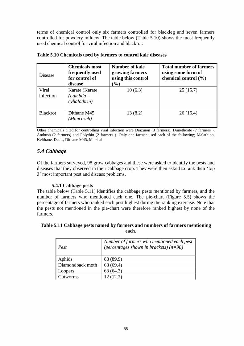
55

terms of chemical control only six farmers controlled for blackleg and seven farmers

controlled for powdery mildew. The table below (Table 5.10) shows the most frequently

used chemical control for viral infection and blackrot.

Table 5.10 Chemicals used by farmers to control kale diseases

Disease

Chemicals most

frequently used

for control of

disease

Number of kale

growing farmers

using this control

(%)


using some form of


Viral

infection

Karate (Karate

(Lambda –

cyhalothrin)

10 (6.3) 25 (15.7)

Blackrot Dithane M45

(Mancozeb)

13 (8.2) 26 (16.4)

Other chemicals cited for controlling viral infection were Diazinon (3 farmers), Dimethoate (7 farmers ),

Ambush (2 farmers) and Polythin (2 farmers ). Only one farmer used each of the following; Malathion,

Kelthane, Decis, Dithane M45, Marshall.

5.4 Cabbage

Of the farmers surveyed, 98 grow cabbages and these were asked to identify the pests and

diseases that they observed in their cabbage crop. They were then asked to rank their „top

3‟ most important pest and disease problems.

5.4.1 Cabbage pests

The table below (Table 5.11) identifies the cabbage pests mentioned by farmers, and the




farmers.

Table 5.11 Cabbage pests named by farmers and numbers of farmers mentioning

each.

Pest

Number of farmers who mentioned each pest


Aphids 88 (89.9)

Diamondback moth 68 (69.4)

Loopers 63 (64.3)

Cutworms 12 (12.2)

56

Aphids, diamondback moth and loopers were the most frequently mentioned cabbage

pests by farmers.

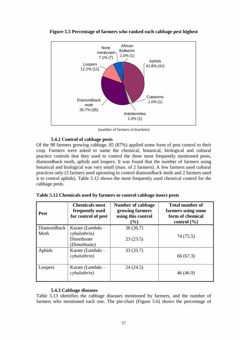
57

Figure 5.5 Percentage of farmers who ranked each cabbage pest highest

Cutworms

1.0% (1)

Ants/termites

1.0% (1)

Aphids

41.8% (41)

African

Bollworm

1.0% (1)

Loopers

12.2% (12)

Diamondback

moth

35.7% (35)

None

mentioned

7.1% (7)


5.4.2 Control of cabbage pests

Of the 98 farmers growing cabbage, 85 (87%) applied some form of pest control to their

crop. Farmers were asked to name the chemical, botanical, biological and cultural

practice controls that they used to control the three most frequently mentioned pests,

diamondback moth, aphids and loopers. It was found that the number of farmers using

botanical and biological was very small (max. of 2 farmers). A few farmers used cultural

practices only (3 farmers used uprooting to control diamondback moth and 2 farmers used

it to control aphids). Table 5.12 shows the most frequently used chemical control for the

cabbage pests.

Table 5.12 Chemicals used by farmers to control cabbage insect pests

Pest

Chemicals most

frequently used

for control of pest

Number of cabbage

growing farmers

using this control

(%)

Total number of

farmers using some

form of chemical

control (%)

Diamondback

Moth

Karate (Lambda –

cyhalothrin)

Dimethoate

(Dimethoate)

36 (36.7)

23 (23.5) 74 (75.5)


cyhalothrin)

33 (33.7)

66 (67.3)

Loopers Karate (Lambda –

cyhalothrin)

24 (24.5)

46 (46.9)

5.4.3 Cabbage diseases

Table 5.13 identifies the cabbage diseases mentioned by farmers, and the number of

farmers who mentioned each one. The pie-chart (Figure 5.6) shows the percentage of

58

farmers who ranked each disease highest. Note that the diseases not mentioned in the

chart were therefore ranked highest by none of the farmers.

Table 5.13 Cabbage diseases named by farmers and numbers of farmers mentioning

each

Disease

Number of farmers who mentioned each

disease (percentages shown in brackets) (n=98)


Blackleg 43 (43.9)

Blackrot 40 (40.8)

Powdery Mildew 3 (3.1)

Figure 5.6 Percentage of farmers who ranked each cabbage disease highest

Viral infection

22.4% (22)

Blackrot

25.5% (25)

Powdery

mildew

1.0% (1)

Bacterial wilt

1.0% (1)

Leaf spot

1.0% (1)

Blackleg

20.4% (20)

None

mentioned

28.6% (28)


5.4.4 Control of cabbage diseases

Only 54% of cabbage farmers said that they apply some form of disease control to their

crop. They were asked to name the chemical, botanical, biological and cultural practice

controls that they used to control four of the most frequently mentioned diseases, viral

infection, blackrot, blackleg and powdery mildew. It was found that few farmers (max. 2)

were using botanical or biological controls. The numbers of farmers using cultural

practices to control for diseases was also low, although it is worth noting that 7 of the

farmers used uprooting to control for blackrot and 3 farmers used this practice to control

viral infection. In terms of chemical control only seven farmers controlled for blackleg

and ten farmers controlled for powdery mildew. The table below (Table 5.14) shows the

most frequently used chemical control for viral infection and blackrot.

59

Table 5.14 Chemicals used by farmers to control cabbage diseases

5.5 Cost of crop protection

Farmers were asked to estimate the amount of money they spent on crop protection for

the last crop of tomato kale and cabbage. Figure 5.7 shows the average cost per hectare of

crop protection for each crop in each district. The cost of crop protection varied by crop

and location (district). The cost of protecting a tomato crop is generally much higher

(£270-390) than the cost of protecting brassicas (£90-240).

Figure 5.7 Cost of crop protection for the last crop by district (£/hectare)

Disease

Chemicals most

frequently used

for control of

Number of cabbage

growing farmers

using this control

(%)

Total number of

farmers using some

form of chemical

control (%)

Blackrot Dithane M45

(Mancozeb)

11 (11.2) 24 (24.5)

60

5.6 Conclusions

African bollworm, aphids and Root knot nematodes were the priority pests in tomatoes

while blight was the highest ranked disease by the majority of farmers. Other pests and

diseases included Red spider mites, leaf minors, cutworms, bacterial wilt, fusarium wilt

and viral infections. Application of chemical pesticides was the main control strategy for

these pests. Farmers used Karate and Dimethoate to control African bollworm and

Aphids. In addition to the 2 chemicals named above, Diazinon was also used to control

Aphids while Furadan is used to control nematodes. To control blights, farmers spray

Dithane and Ridomil.

Aphids, DBM and loopers are the most important pests of kale and cabbage. In addition,

viral infection and blackrot are the most frequently mentioned diseases of kale and

cabbage. In addition to the above, cutworms, African bollworm, spider mites and root

knot nematodes are also mentioned by farmers. Notably, viral infection is ranked highest

by the majority of kale farmers. Most farmers spray Karate to control DBM aphids and

loopers.

Out of the 200 farmers surveyed, only 1-5 cited use of botanicals to control vegetable

pests. 99% of the peri-urban vegetable farmers employ chemical control strategies for

pests and diseases. Surprisingly farmers use Karate to control viral infection. This

possibly reflects farmer ability to link viral infection with arthropod pests, which are

vectors of the same. Black rot is controlled by Dithane M45. The other surprising result

was that weeds were not specifically mentioned as a pest or constraint. Being a labour

requiring activity, this finding perhaps reflects availability of affordable labour

throughout the cropping season in the peri-urban vegetable production system.

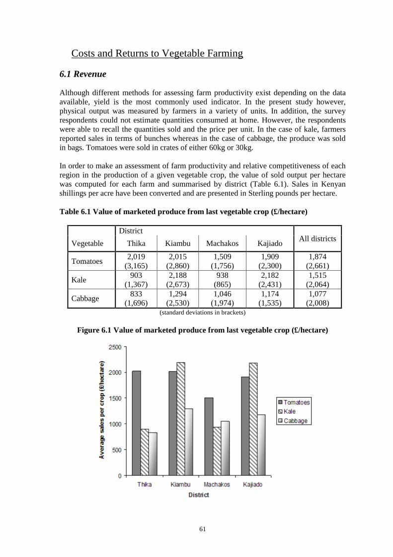
61

Costs and Returns to Vegetable Farming

6.1 Revenue

Although different methods for assessing farm productivity exist depending on the data

available, yield is the most commonly used indicator. In the present study however,

physical output was measured by farmers in a variety of units. In addition, the survey

respondents could not estimate quantities consumed at home. However, the respondents

were able to recall the quantities sold and the price per unit. In the case of kale, farmers

reported sales in terms of bunches whereas in the case of cabbage, the produce was sold

in bags. Tomatoes were sold in crates of either 60kg or 30kg.

In order to make an assessment of farm productivity and relative competitiveness of each

region in the production of a given vegetable crop, the value of sold output per hectare

was computed for each farm and summarised by district (Table 6.1). Sales in Kenyan

shillings per acre have been converted and are presented in Sterling pounds per hectare.

Table 6.1 Value of marketed produce from last vegetable crop (£/hectare)

District All districts

Vegetable Thika Kiambu Machakos Kajiado

Tomatoes 2,019

(3,165)

2,015

(2,860)

1,509

(1,756)

1,909

(2,300)

1,874

(2,661)

Kale 903

(1,367)

2,188

(2,673)

938

(865)

2,182

(2,431)

1,515

(2,064)

Cabbage 833

(1,696)

1,294

(2,530)

1,046

(1,974)

1,174

(1,535)

1,077

(2,008) (standard deviations in brackets)

Figure 6.1 Value of marketed produce from last vegetable crop (£/hectare)

62

Revenue from kale sales varies between districts with sample farms in Thika and

Machakos generating around £1000 per hectare. This value doubles to £2000 in the case

of Kiambu and Kajiado farms. Revenue per hectare of tomatoes varies from £1500 in

Machakos to £2000 Thika, Kiambu and Kajiado. Compared to kale and tomatoes,

revenues per hectare from cabbage are lowest in all districts except Machakos.

Noteworthy however, are the large standard deviations indicating variations within

districts (Table 6.1).

6.2 Returns to vegetable farming

The value of sold products gives an indication of productivity. However, gross margin

(total revenue - total variable cost) provides a clearer picture of the relative profitability of

a given enterprise. Gross margins can also be used to assess the relative competitiveness

of a given enterprise. Of more relevance to the present study is the proportion of total

variable cost attributable to pest control in vegetables given that farmers rank pests and

diseases as the main constraint to expanded vegetable production. In order to delineate the

variable costs, the whole production process is analysed. Prior to the farm household

survey, focus group interviews were conducted in Kiambu and Machakos where farm

enterprise budgets were developed for tomatoes and the brassicas, through a participatory

budgeting exercise. The production process for each crop was therefore studied in detail

and monetary values for activities not captured in the individual household survey were

documented. Both the focus group interviews and the individual farm surveys revealed

that peri-urban vegetable farmers employ both hired and family labour in most farm

operations. Labour requiring activities include nursery preparation and management,

seedbed and basin preparation, irrigation, weeding, fertilizer application, spraying,

pruning, staking, mulching, shading and harvesting.

6.2.1 Variable inputs and outputs

The hired labour wage rate is used as the opportunity cost of family labour

Value of seed at the point of purchase is used to estimate the cost of seed

Cost of irrigation includes pump, pipe and labour costs during irrigation

Manure and fertilizer costs are estimated at farm gate

Foliar feed, cost of chemical pesticides are estimated at point of purchase

Outputs measured in terms of value of sold outputs

Different scenarios are presented to reflect different production systems and intensity of

input use. Kiambu area reflects cool highland regions (LH3 and UM4). Machakos and

Kajiado on the other hand lie in the hereafter referred to as “lowland” lie in the hotter and

more arid upper midland 6 (UM 6). Accordingly, Kiambu is selected to represent high

input scenario for tomatoes while Machakos represents a high input system for kale and

cabbage. In this scenario, producers follow all the recommended practices. The variable

costs and revenues indicated are those reported during the participatory budgeting

exercise.

The “lowland” system represents both Machakos and Kajiado. The costs of crop

protection and revenue for each crop are those reported in the individual household

survey. The same applies for Mbagathi area in Thika, which is a unique low input zone

with minimal irrigation cost.

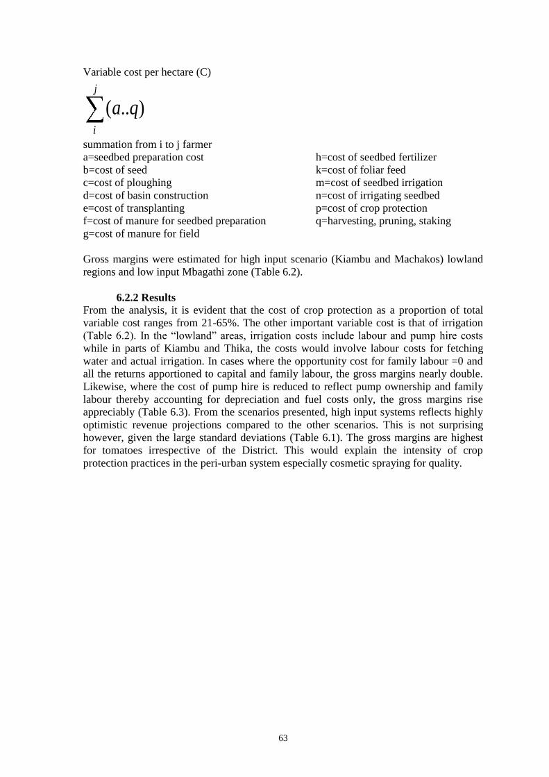
63

Variable cost per hectare (C)

j

i

qa )..(

summation from i to j farmer

a=seedbed preparation cost h=cost of seedbed fertilizer

b=cost of seed k=cost of foliar feed

c=cost of ploughing m=cost of seedbed irrigation

d=cost of basin construction n=cost of irrigating seedbed

e=cost of transplanting p=cost of crop protection

f=cost of manure for seedbed preparation q=harvesting, pruning, staking

g=cost of manure for field

Gross margins were estimated for high input scenario (Kiambu and Machakos) lowland

regions and low input Mbagathi zone (Table 6.2).

6.2.2 Results

From the analysis, it is evident that the cost of crop protection as a proportion of total

variable cost ranges from 21-65%. The other important variable cost is that of irrigation

(Table 6.2). In the “lowland” areas, irrigation costs include labour and pump hire costs

while in parts of Kiambu and Thika, the costs would involve labour costs for fetching

water and actual irrigation. In cases where the opportunity cost for family labour =0 and

all the returns apportioned to capital and family labour, the gross margins nearly double.

Likewise, where the cost of pump hire is reduced to reflect pump ownership and family

labour thereby accounting for depreciation and fuel costs only, the gross margins rise

appreciably (Table 6.3). From the scenarios presented, high input systems reflects highly

optimistic revenue projections compared to the other scenarios. This is not surprising

however, given the large standard deviations (Table 6.1). The gross margins are highest

for tomatoes irrespective of the District. This would explain the intensity of crop

protection practices in the peri-urban system especially cosmetic spraying for quality.

64

Table 6.2 Gross margins analysis for Vegetable production (£/hectare)

CABBAGE KALE TOMATO

Activity Machakos Lowland

areas

Mbagathi Machakos Lowland

areas

Mbagathi Kiambu Lowland

areas

Mbagathi

Seedbed preparation

cost 1.72 1.72 1.72 1.72 1.72 1.72 4.3 4.3 4.3

Cost of seed 5.8 5.8 5.8 5.8 5.8 5.8 10.31 10.31 10.31

Cost of ploughing 32.22 32.22 32.22 32.22 32.22 32.22 21.48 21.48 21.48

Cost of basin

construction 171.83 41.88 41.88 171.83 41.88 41.88 0 0 0

Cost of transplanting 137.46 34.37 34.37 137.46 34.37 34.37 0 0 0

Cost of manure for

seedbed preparation 0.43 0.43 0.43 0.43 0.43 0.43 1.07 1.07 1.07

Cost of manure for

field 15.03 0 15.03 15.03 0 15.03 0 0 0

Cost of seedbed

fertilizer 1.72 1.72 1.72 1.72 1.72 1.72 0.64 0.64 0.64

Cost of foliar feed 40.59 40.6 40.59 40.59 40.6 40.59 0 0 0

Cost of seedbed

irrigation 622.87 622.87 214.78 622.87 622.87 214.78 859.13 644.35 214.78

Cost of crop protection 270.63 190 150 270.63 270.63 270.63 1640.94 343.65 343.65

Variable cost 1300.3 971.61 538.54 1300.3 1052.24 659.17 2537.87 1025.8 596.23

Revenue 4000 1755 903 5000 1560 923.57 8591.3 2028 3065

Cost of protection as a

% of total variable cost

21 20 28 21 26 41 65 34 58

Gross margin 2699.7 783.39 364.46 3699.7 507.76 264.4 6053.43 1002.2 2468.77

Table 6.3 Changes in gross margin when irrigation costs are reduced

Activity Machakos Lowland

areas

Mbagathi Machakos Lowland

areas

Mbagathi Kiambu Lowland

areas

Mbagathi

Cost of seedbed

irrigation 622.87 300 0 622.87 300 0 859.13 300 0

Gross margin 2699.7 1106.26 579.24 3699.7 830.63 479.18 6053.43 1346.55 2683.55

65

6.3 Modelling Determinants of Cost of Pest Control

During the survey, farmers reported expenditure on pest control for the last crop of kale

cabbage and tomatoes. There are wide variations in the reported costs of crop protection.

Nonetheless, the reported costs reflect smallholder vegetable farmer expenditure patterns

on crop protection. These costs exclude the cost of weeding and other transaction cost

elements associated with obtaining crop protection products.

6.3.1 The explanatory variables

Experience in vegetable farming

By and large, experienced vegetable growers should allocate their resources optimally.

On the one hand, they may use more costly and effective pest management strategies in

order to avoid pest resistance. On the other hand, they may adopt cost cutting strategies as

long as they meet product quality dictated by market demand. The expected influence of

experience on pest control expenditures is therefore either positive or negative.

Value of marketed output

In order to capture the price effects, value of output per acre is incorporated as an

explanatory variable. The higher the value of marketed output, the greater the attention to

pest management problems, which translates to higher expenditure given the importance

of pests and diseases.

Total farm area

Total farm area refers to the cropped and non-cropped areas. Owners of large land

holdings tend to be wealthier and may spend more on pest management practices.

Level of formal education

Previous adoption studies have shown that education level influences adoption of new

innovations especially complex technologies. Furthermore, the majority of survey

respondents apply chemical control strategies. It is hypothesised that a high level of

formal education has similar influence on pest management expenditure to that of

experience.

Region of production

Agro-climatic factors are also hypothesised to influence the cost of pest management.

Previous studies in the peri-urban vegetable systems indicated that Kajiado and Machakos

areas have a high incidence of vegetable pests and diseases.

6.3.2 Estimation

It was hypothesised that expenditure on crop protection is influenced by a number of

factors, generally expressed as follows.

66

COST ƒ (PERIOD, YIELD, TERTIARY, REGION, FARM)

COST= expenditure on crop protection for the last kale, cabbage or tomato crop in Kenya

shillings

PERIOD= the period for which the farmer has been growing vegetables in years

YIELD=value of marketed output per acre grown of kale, cabbage or tomato respectively

FARM =Total farm area in acres

TERTIARY= Level of formal education; 1= at least secondary level of education; 0

otherwise

REGION= Production zone; “Lowland”=1; 0 otherwise

The model was estimated for kale, cabbage and tomato using Ordinary Least Squares

Regression procedure in the Statistical Package for Social Sciences (SPSS).

The reported cost of crop protection for tomato kale and cabbage for the last crop was

taken as the dependent variable. This model explains 21%, 26% and 37% of the variations

in expenditure on crop protection on tomato, kale and cabbage respectively. In the case of

tomatoes, the “lowland” region (comprising Kajiado and Machakos), at least secondary

school level of education, total farm area and period of growing vegetables have a

significant positive influence on crop protection expenditure. In the case of kale, only

region and education level have a significant positive influence while for cabbage, total

farm area, formal education level and region all have a positive and significant effect

(Table 6.5).

6.3.4 Discussion

These findings indicate that location of farms in Kajiado and Machakos has a positive

influence on crop protection expenditure for kale, cabbage and tomatoes compared to

farms in Thika and Kiambu. A possible reason could be higher incidence of pests and

diseases in these areas or the nature of pests and diseases that require more costly

chemical pesticides to control.

Although farm operators in Machakos have attained higher levels of formal education

than the rest of the sample, this effect is not significant when they are combined with

farm operators from Kajiado. A test for multicollinearity between education level and

region revealed a weak linear association (correlation coefficient of 0.1). Across the

sample farms therefore, farm operators educated to secondary school and above spend

more on crop protection than their counterparts with lower level of education. These

operators are probably more aware of the crop protection needs and therefore employ

more costly strategies.

Total farm area can be used as a proxy for wealth status especially in the peri-urban

Nairobi. Large farm owners are better endowed with resources and can afford timely

purchase of chemical pesticides used by the majority of the peri-urban farmers. This

could be more relevant in the case of tomatoes where the proportion of variable cost

attributable to pest management is generally higher. In the case of cabbage, a crop that is

harvested once as compared to tomatoes and kale that are harvested over a period of time,

there would seem to be a minimum area of land below which it is uneconomical to plant

cabbage. Table.4.3. indicates that the cropped area for cabbage is on average higher than

67

that for tomato and kale and kale. The larger the area planted therefore, the greater the

cost of crop production.

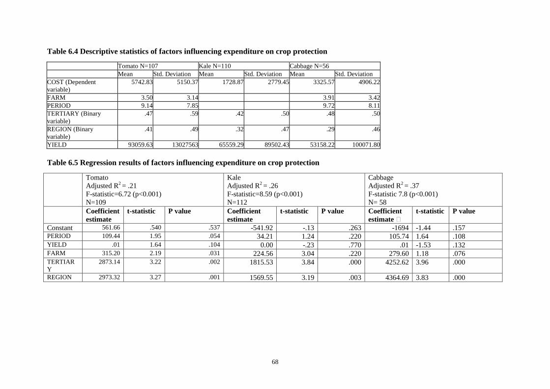
68

Table 6.4 Descriptive statistics of factors influencing expenditure on crop protection

Tomato N=107 Kale N=110 Cabbage N=56

Mean Std. Deviation Mean Std. Deviation Mean Std. Deviation

COST (Dependent

variable)

5742.83 5150.37 1728.87 2779.45 3325.57 4906.22

FARM 3.50 3.14 3.91 3.42

PERIOD 9.14 7.85 9.72 8.11

TERTIARY (Binary

variable)

.47 .59 .42 .50 .48 .50

REGION (Binary

variable)

.41 .49 .32 .47 .29 .46

YIELD 93059.63 13027563 65559.29 89502.43 53158.22 100071.80

Table 6.5 Regression results of factors influencing expenditure on crop protection

Tomato

Adjusted R2 = .21

F-statistic=6.72 (p<0.001)

N=109

Kale

Adjusted R2 = .26

F-statistic=8.59 (p<0.001)

N=112

Cabbage

Adjusted R2 = .37

F-statistic 7.8 (p<0.001)

N= 58

Coefficient

estimate

t-statistic P value Coefficient

estimate

t-statistic P value Coefficient

estimate

t-statistic P value

Constant 561.66 .540 .537 -541.92 -.13 .263 -1694 -1.44 .157 PERIOD 109.44 1.95 .054 34.21 1.24 .220 105.74 1.64 .108 YIELD .01 1.64 .104 0.00 -.23 .770 .01 -1.53 .132 FARM 315.20 2.19 .031 224.56 3.04 .220 279.60 1.18 .076 TERTIAR

Y

2873.14 3.22 .002 1815.53 3.84 .000 4252.62 3.96 .000

REGION 2973.32 3.27 .001 1569.55 3.19 .003 4364.69 3.83 .000

69

References

Cooper, J. (1999). Pest management in horticultural crops; integrating sustainable pesticide

use into biocontrol-based peri-urban production systems in Kenya. Final Technical Report, R

6616.

FAO (1999). Urban and Peri-urban Agriculture. Report (COAG/99/10) to the FAO

Committee on Agriculture, Rome, 25-26 January 1999.

Jaetzhold, R. and R. Schmidt (1983a) Farm Management Handbook of Kenya Volume II B

Central Kenya. Ministry of Agriculture, Kenya in Cooperation with the German Agricultural

Team and the German Agency for Technical Cooperation (GTZ)

Jaetzhold, R. and R. Schmidt (1983b) Farm Management Handbook of Kenya Volume II C

East Kenya. Ministry of Agriculture, Kenya in Cooperation with the German Agricultural

Team and the German Agency for Technical Cooperation (GTZ)

Kamau, M. and B. Mills (1998) Technology, Location and Trade: Kenyan vegetables . In;

Mills B. (Ed)s. Agricultural Research. Priority Setting. Information Investment for the

Improved use of Research Resources. International Service for National agricultural Research

ISBN 92-9118-040-8.

Odour, G.; Ong‟aro, J.; Pete, S.; Karanja, P.; Cooper, J.; Mwaniki, S. Kibata, G. N.; Simons,

S. A. 1998. Pests of horticultural crops on small-scale peri-urban farms in Nyathuna,

Kiambu: influence of pesticide regimes on pests and natural enemies. In Proceedings of the

Second Biennial Crop Protection Conference held from 16-17 September, KARI /DFID, p.

18-29

Otieno Oruko, L. Asaba, J.F. and Kindness, H.M. (2000) Factors affecting uptake and

adoption of outputs of crop protection research in peri-urban vegetable systems in Kenya

pp.27-34, In: Sustaining change: proceedings of a workshop on the factors affecting uptake

and adoption of Department for International Development (DFID) Crop Protection

Programme (CPP) research outputs. Hainsworth, S.D. and Eden-Green, S.J. (Ed.). Imperial

College at Wye, Kent, UK. 21-23 June 2000. Natural Resources International, Chatham

Maritime, Kent, UK. 160 pp. ISBN 0-9539274-0-7.

Republic of Kenya (1997) National Development Plan 1997-2001. Government Printer

Nairobi.

Republic of Kenya (1999) Economic Survey 1999. Office of the Vice President and Ministry

of Planning and National Development. Central Bureau of Statistics.

http:// http://www.nrinternational.co.uk/cpppc/1.htm.

http://www.nrinternational.co.uk/cpppc/1.htm

70

70

Annex 1: Questionnaire for vegetable grower characteristics survey July-August

2000

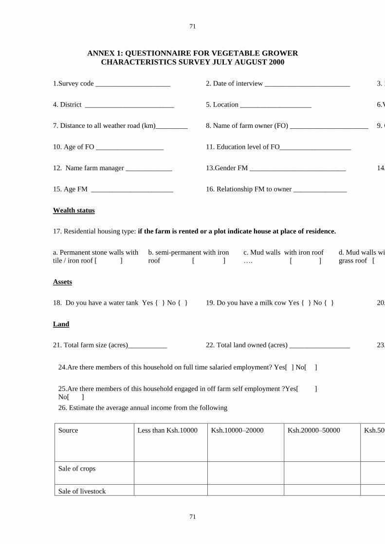
71

71

ANNEX 1: QUESTIONNAIRE FOR VEGETABLE GROWER

CHARACTERISTICS SURVEY JULY AUGUST 2000

1.Survey code _____________________ 2. Date of interview ________________________ 3. Enumerator ________________________

4. District _________________________ 5. Location ____________________ 6.Village _____________________________

7. Distance to all weather road (km)_________ 8. Name of farm owner (FO) ______________________ 9. Gender of FO __________________

10. Age of FO ___________________ 11. Education level of FO____________________

12. Name farm manager _____________ 13.Gender FM ___________________________ 14. Education level of FM ________________

15. Age FM _______________________ 16. Relationship FM to owner _______________

Wealth status

17. Residential housing type: if the farm is rented or a plot indicate house at place of residence.

a. Permanent stone walls with

tile / iron roof [ ]

b. semi-permanent with iron

roof [ ]

c. Mud walls with iron roof

…. [ ]

d. Mud walls with makuti/

grass roof [ ]

e. Timber house with cement

floor [ ]

Assets

18. Do you have a water tank Yes { } No { } 19. Do you have a milk cow Yes { } No { } 20. Do you own a vehicle Yes =1 No=0

Land

21. Total farm size (acres)___________ 22. Total land owned (acres) _________________ 23. Value of land owned Ksh _____________

24.Are there members of this household on full time salaried employment? Yes[ ] No[ ]

25.Are there members of this household engaged in off farm self employment ?Yes[ ]

No[ ]

26. Estimate the average annual income from the following

Source Less than Ksh.10000 Ksh.10000–20000 Ksh.20000–50000 Ksh.50000–100000 Over Ksh100000

Sale of crops

Sale of livestock

72

72

products

Off farm salaried

employment

Off farm self

employment

27. Do you get remittances from off-farm activities for investment on farm activities? Yes[ ] No[ ]

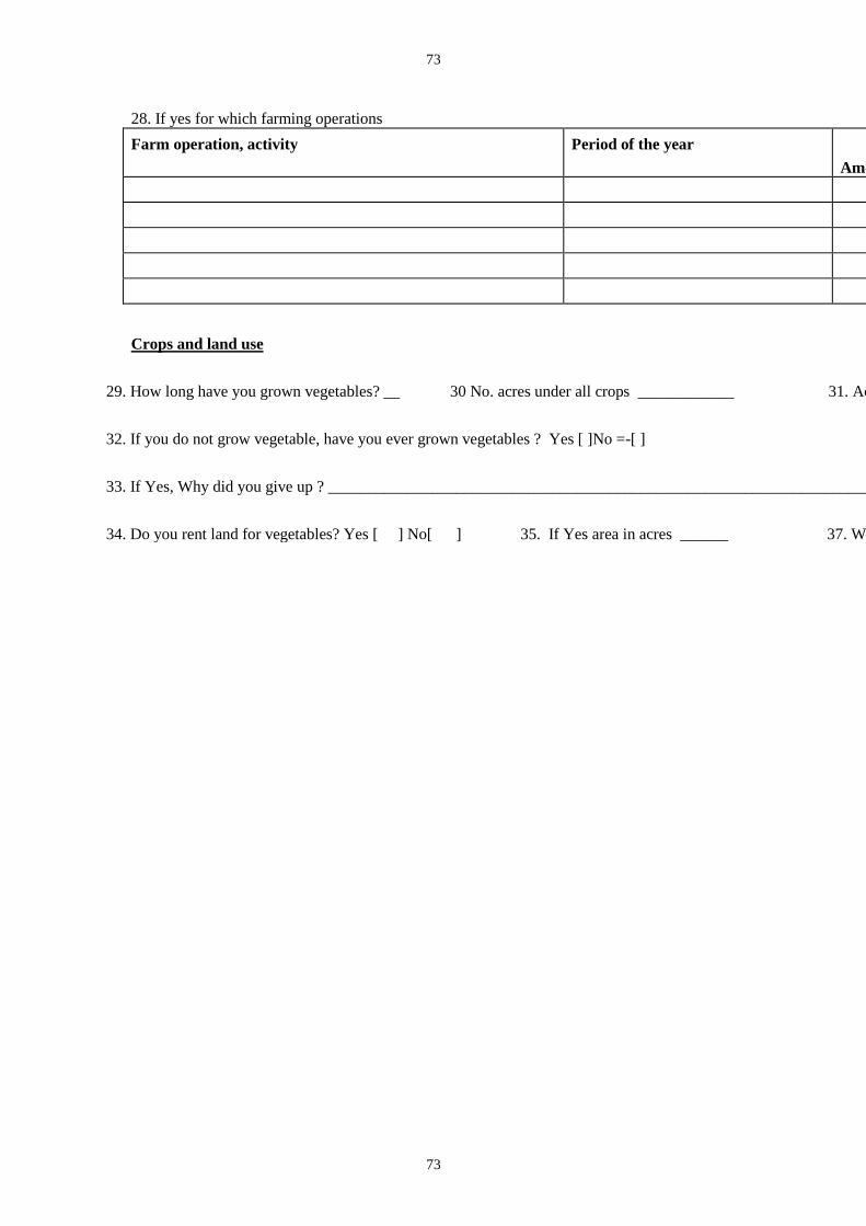
73

73

28. If yes for which farming operations

Farm operation, activity Period of the year

Amount Ksh

Crops and land use

29. How long have you grown vegetables? __ 30 No. acres under all crops ____________ 31. Acres now under vegetable _______

32. If you do not grow vegetable, have you ever grown vegetables ? Yes [ ]No =-[ ]

33. If Yes, Why did you give up ? _________________________________________________________________________________________

34. Do you rent land for vegetables? Yes [ ] No[ ] 35. If Yes area in acres ______ 37. What is the rental value Ksh ________

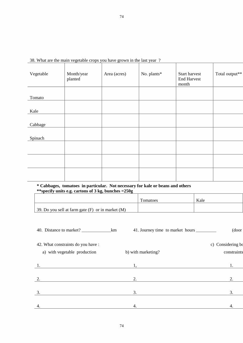
74

74

38. What are the main vegetable crops you have grown in the last year ?

Vegetable Month/year

planted

Area (acres) No. plants* Start harvest

End Harvest

month

Total output** Quantity sold Value of sales

Price x Untie

Tomato

Kale

Cabbage

Spinach

* Cabbages, tomatoes in particular. Not necessary for kale or beans and others

**specify units e.g. cartons of 3 kg, bunches =250g

Tomatoes Kale Cabbage Spinach

39. Do you sell at farm gate (F) or in market (M)

40. Distance to market? _____________km 41. Journey time to market hours _________ (door to place of sale)

42. What constraints do you have : c) Considering both production and market

a) with vegetable production b) with marketing? constraints rank the most important

1. 1, 1.

2. 2. 2.

3. 3. 3.

4. 4. 4.

75

75

43. Vegetable seed variety and seed source used in the last year

Vegetable Seed source Variety

Tomato 1

2

1 Cal-J

2. RIO GRANDE

Kale 1

2

1

2

Cabbage 1

2

1

2

Spinach 1

2

1

2

44. Do you grow any of your own seed ? Yes { } No { }

45. If yes, for which vegetable (s) ____________________________________________________________________________________

46. Why? _________________________________________________________________________________________________________

Pest and diseases control (show a picture or sample of the pest, or disease)

47 a. What are the main pests you have in Kale cabbage and tomatoes?

b. Which are the main diseases you have in Kale cabbage and tomatoes?

…..c For each crop (cabbage, kale and tomatoes) considering both pests and diseases rank

the 3 most important problems

Vegetable Pest Rank Disease Rank

Tomato

1.African bollworm 1 Blight

2.Aphids 2 Bacterial wilt

3.Leaf miner 3 Fusarium wilt

4. Nematodes

Kales

1.Diamondback moth 1. Blackrot

2. Aphids 2. Virus

3.Looper 3. Blackleg

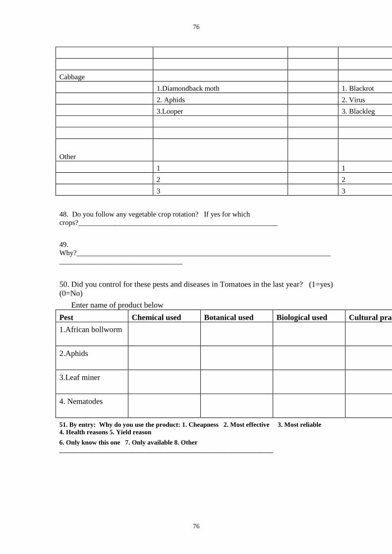
76

76

Cabbage

1.Diamondback moth 1. Blackrot

2. Aphids 2. Virus

3.Looper 3. Blackleg

Other

1 1

2 2

3 3

48. Do you follow any vegetable crop rotation? If yes for which

crops?_______________________________________________________

49.

Why?______________________________________________________________________

__________________________________

50. Did you control for these pests and diseases in Tomatoes in the last year? (1=yes)

(0=No)

Enter name of product below

Pest Chemical used Botanical used Biological used Cultural practice Others

1.African bollworm

2.Aphids

3.Leaf miner

4. Nematodes

51. By entry: Why do you use the product: 1. Cheapness 2. Most effective 3. Most reliable

4. Health reasons 5. Yield reason

6. Only know this one 7. Only available 8. Other

_________________________________________________________________

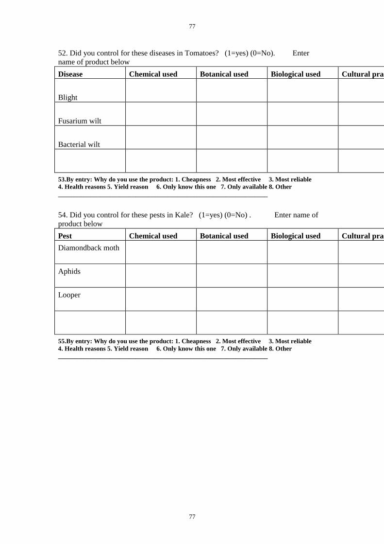
77

77

52. Did you control for these diseases in Tomatoes? (1=yes) (0=No). Enter

name of product below

Disease Chemical used Botanical used Biological used Cultural practice Others

Blight

Fusarium wilt

Bacterial wilt

53.By entry: Why do you use the product: 1. Cheapness 2. Most effective 3. Most reliable

4. Health reasons 5. Yield reason 6. Only know this one 7. Only available 8. Other

_________________________________________________________________

54. Did you control for these pests in Kale? (1=yes) (0=No) . Enter name of

product below


Diamondback moth

Aphids

Looper



_________________________________________________________________

78

78

56. Did you control for these diseases in kale? (1=yes) (0=No) . Enter name of

product below


Blackrot

Virus

Blackleg

Powdery mildew


4. Health reasons 5. Yield reason 6. Only know this one 7. Only available 8. Other _________________________________________________________________

58. Did you control for these pests in cabbage? (1=yes) (0=No). Enter name of

product below


Diamondback moth

Aphids

Looper

59. By entry: Why do you use the product: 1. Cheapness 2. Most effective 3. Most reliable


_________________________________________________________________

60. Did you control for these diseases in cabbages? (1=yes) (0=No). Enter name

of product below


Blackrot

Virus

79

79

Blackleg

Downy mildew



_________________________________________________________________

62. Have you changed any of the following practices in the last 3 years ? If yes

why?

Practice No / Yes If yes, which ? Why? Give reason

Stopped growing a particular crop

Stopped using any product

Stopped a rotation

Stopped other cultural method

Started growing a particular crop

Started using any different product

Started a different rotation

Started using a new cultural method

Tomato Kale Cabbage Spinach

63. Do you know how much you spent on each crop on

crop protection last crop ?* Enter Ksh

* If producers do not know these then record not known

64. Do you own a knapsack sprayer Yes { } No{ } 65 If No, how do you apply chemicals or botanicals ________________________________

66. Do you irrigate Yes{ }No {….}

67. If Yes, how did you irrigate?

1. From river, pumped, overhead irrigation

2. From river, pumped, hose / basin irrigation

3. From river, channels and gravity

4. From own well, by hand

5. From communal well, by hand

6. From river, by hand

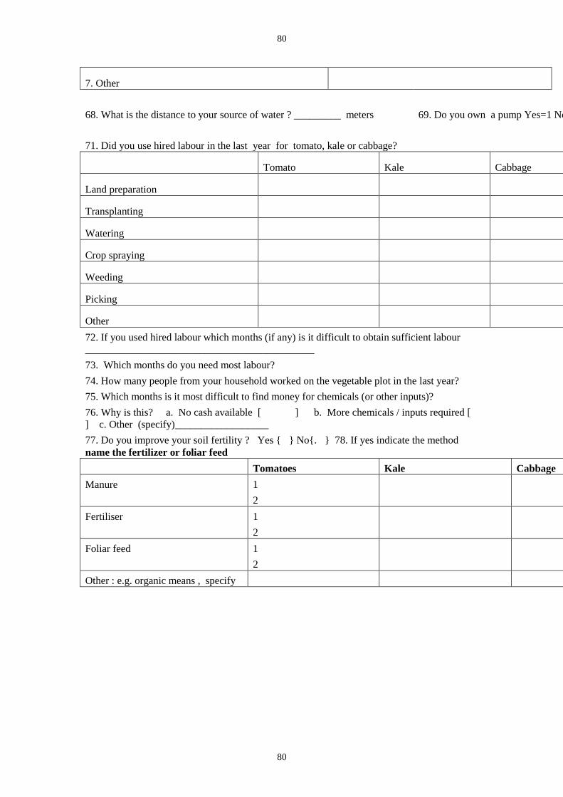
80

80

7. Other

68. What is the distance to your source of water ? _________ meters 69. Do you own a pump Yes=1 No=0 70. Do you hire a pump? Yes=1 No=0

71. Did you use hired labour in the last year for tomato, kale or cabbage?

Tomato Kale Cabbage Spinach

Land preparation

Transplanting

Watering

Crop spraying

Weeding

Picking

Other

72. If you used hired labour which months (if any) is it difficult to obtain sufficient labour

____________________________________________

73. Which months do you need most labour?

74. How many people from your household worked on the vegetable plot in the last year?

75. Which months is it most difficult to find money for chemicals (or other inputs)?

76. Why is this? a. No cash available [ ] b. More chemicals / inputs required [

] c. Other (specify)__________________

77. Do you improve your soil fertility ? Yes { } No{. } 78. If yes indicate the method

name the fertilizer or foliar feed

Tomatoes Kale Cabbage Spinach

Manure 1

2

Fertiliser 1

2

Foliar feed 1

2

Other : e.g. organic means , specify

81

81

FIELD TRIAL REPORT MARK PARNELL DRAFT

Field trials of Plutella xylostella granulovirus against diamondback moth on kale,

carried out in Kenya 2000 and 2001.

Summary

Brassica crops are important foods source for the urban populations in Kenya and

their production is a major income generator for many small scale growers around

towns. The development of insecticide resistance by the key pest, diamond back

moth (DBM), currently threatens the sustainability of production thus new and

improved technologies are required. Plutella xylostella granulovirus (PlxyGV) has

shown promise for DBM control in other countries and in past field trials in Kenya

and may be an important alternative to chemical control in the future.

Field trials were carried out from February to August 2000 (long rains) and

September 2000 to January 2001 (short rains) in order to ascertain the lowest dose of

PlxyGV required to control DBM on small plots of kale established on research

station ground at two sites in and around Nairobi, Kenya. Results showed that

PlxyGV performed significantly better than chemical control in reducing DBM

populations and increasing kale yield over a growing season. Up to 30% increase in

yield was observed in PlxyGV plots when compared to the control or chemical over

the growing seasons, a very encouraging initial result for an un-formulated, crude

extract. The results have also shown that to provide adequate control of DBM

populations a dose rate of 3.0x1014

occlusion bodies per hectare would be required.

Such a dose-rate is equivalent to 7500 larvae per hectare.

Introduction

Project R7449 evaluation and promotion of biorational control of Plutella xylostella,

the diamond back moth (DBM), is a three year follow-on project from project R6615

that was set up to develop alternatives to chemical control of DBM in Kenya. The

specific target group of the project is smallholder Kenyan farmers growing vegetables

belonging to the Brassica family, the preferred diet of DBM. The project is being

carried out in collaboration with the Kenyan Agricultural Research Institute (KARI),

CAB International Africa Regional Centre (CABI-ARC) and Horticulture Research

International (HRI) based in the UK. This report specifically concerns trials to

develop the use of Plutella xylostella granulovirus (PlxyGV) against DBM on kale

and discusses work carried out during two growing seasons, the long rains season of

February to August 2000 and the short rains season of September 2000 to January

2001.

PlxyGV can be applied to crops in much the same was as conventional insecticides

using existing spray application technology of the small or large-scale farmer. To this

end it has great advantages for adoption by farming communities. Its mode of action

is by stomach poisoning and successful infection requires the high pH environment of

its host's midgut in order to release virus particles from protective occlusion bodies.

PlxyGV is host specific and has shown no effect on organisms other than DBM.

82

82

There are no commercially available PlxyGV-based products. Therefore the material

used in the trials was produced in country by CABI-ARC staff in laboratories at their

regional centre in the ICRAF Complex, Nairobi. The virus produced had been sent to

the UK and bioassayed at NRI to check its efficacy in lab culture insects using a leaf-

dip bioassay method.

Studies carried out in 1998 under the previous phase of the project to identify

alternatives to chemical control of DBM (R6615) had shown that PlxyGV was

significantly better than chemical pesticide (Karate) in controlling pest populations

and damage level in kale (Parnell 1999). In that study PlxyGV had been applied at

dose rates of 3.0x1013

and 3.0x1014

OB/ha. Although significant differences occurred

between PlxyGV, control and chemical, no significant differences were observed in

damage or DBM population between the two dose rates of PlxyGV. The purpose of

the current study was therefore to identify the lowest dose possible to achieve

adequate control and also to obtain data on the effect of treatments on harvest levels

throughout a growing season of kale.


The PlxyGV dose rate trials consisting of five treatments replicated four times were

set-up at two separate locations in and around Nairobi in two different growing

seasons. At both times one trial site was established at the National Agricultural

Research Laboratories (NARL) in Nairobi and the other was on research land owned

by KARI-Thika 60 km north of Nairobi just outside Thika Town. The test crop for

the trial was kale at both sites and treatments were allocated in a complete random

block design. The following treatments were included in the trial

T1: 3 x 1012

of GV (in 0.02% Triton X100)

T2: 3 x 1013


T3: 3 x 1014


T4: Karate

T5: Control (0.02% Triton X100)

All were applied using lever operated knapsack sprayers at a volume application rate

of 1000 litres/hectare. Figure 1 shows the site design for both field sites.

Figure 1. Field site design for field trials in Kenya, February to August 2000.

83

83

Road side

28 m

8 rows of

9 plants in

each plot.

T4

4.8m 5.2m

T5 T1 T2 T3

1m gaps between plots

T3 T4 T2 T5 T1

24.6 m

T4 T3 T5 T2 T1

T2 T5 T1 T3 T4

Each treatment was applied following good spraying practice guidelines set out by

IPARC (Matthews, 1992). Before spraying commenced, all equipment was calibrated

to ensure accurate application of NPV and spray procedures followed standard

practice. Volume application rate of all treatments was 2 litres per plot.

Monitoring of the trial was carried out in the following way

10 plants in the central area of the plot (guard rows at edges) were sampled

weekly for numbers of DBM larvae present, damage caused by DBM and number

of GV infected DBM.

At sampling, a number of apparently infected dead larvae were collected for later

confirmation that they were GV killed.

Yield data was collected for weight of harvest and the percent marketable at

regular intervals and a clear note was made of the days harvesting was done in

order to account for sudden drops in DBM population due to removal.

In an independent experiment to compare observed infection in the field to final

infection of observed larvae, one plot of kale 5m x 5m was sprayed with the medium

dose virus. After four days, between 30 and 50 larvae of 1st 2

nd, 3

rd, and 4

th instar were

collected from the plants and taken to the lab for rearing on to observe level of

infection. A record was made of the number of collected larvae showing virus

symptoms at collection and subsequently GV infection was recorded 5, 7 and 9 days

post collection.

Results

84

84

Field Inoculum

The LC50 value of the field inoculum produced by CABI-ARC staff was 1.90x107

OB/ml. See Figure 2.

Figure 2. Dose response curve of second instar DBM to PlxyGV produced at

CABI-ARC for the year 2000 field trials.

Log10 dose (OB/ml)

105 106 107 108 109

% Mortality

0

10

20

30

40

50

60

70

80

90

100

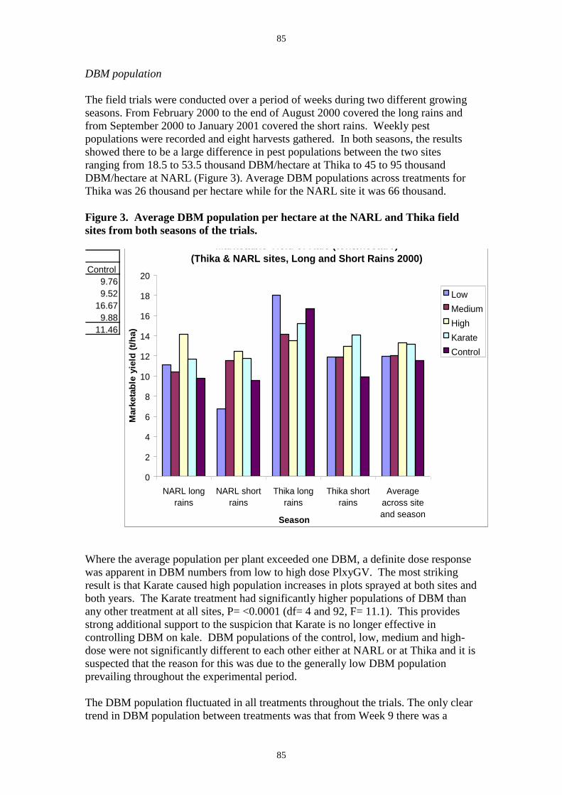
85

85

DBM population

The field trials were conducted over a period of weeks during two different growing

seasons. From February 2000 to the end of August 2000 covered the long rains and

from September 2000 to January 2001 covered the short rains. Weekly pest

populations were recorded and eight harvests gathered. In both seasons, the results

showed there to be a large difference in pest populations between the two sites

ranging from 18.5 to 53.5 thousand DBM/hectare at Thika to 45 to 95 thousand

DBM/hectare at NARL (Figure 3). Average DBM populations across treatments for

Thika was 26 thousand per hectare while for the NARL site it was 66 thousand.

Figure 3. Average DBM population per hectare at the NARL and Thika field

sites from both seasons of the trials.

Where the average population per plant exceeded one DBM, a definite dose response

was apparent in DBM numbers from low to high dose PlxyGV. The most striking

result is that Karate caused high population increases in plots sprayed at both sites and

both years. The Karate treatment had significantly higher populations of DBM than

any other treatment at all sites, P= <0.0001 (df= 4 and 92, F= 11.1). This provides

strong additional support to the suspicion that Karate is no longer effective in

controlling DBM on kale. DBM populations of the control, low, medium and high-

dose were not significantly different to each other either at NARL or at Thika and it is

suspected that the reason for this was due to the generally low DBM population

prevailing throughout the experimental period.

The DBM population fluctuated in all treatments throughout the trials. The only clear

trend in DBM population between treatments was that from Week 9 there was a

Control

9.76

9.52

16.67

9.88

11.46

Marketable Yield of Kale (tons/hectare)

(Thika & NARL sites, Long and Short Rains 2000)

0

2

4

6

8

10

12

14

16

18

20

NARL long

rains

NARL short

rains

Thika long

rains

Thika short

rains

Average

across site

and seasonSeason

Mark

eta

ble

yie

ld (

t/h

a)

Low

Medium

High

Karate

Control

0

2

4

6

8

10

12

14

16

18

20

Low

Long

Rains

2000

High Control Medium Karate

Mark

eta

ble

yie

ld (

t/h

a)

Thika

NARL

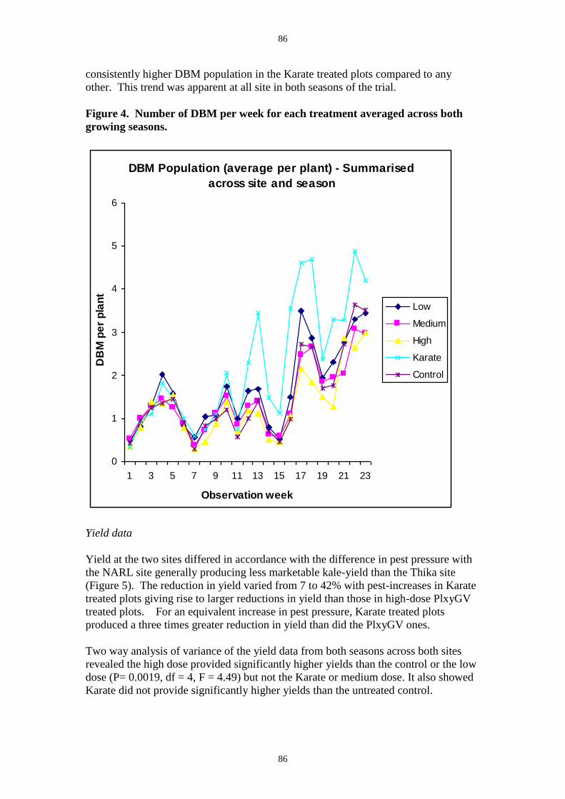
86

86

consistently higher DBM population in the Karate treated plots compared to any

other. This trend was apparent at all site in both seasons of the trial.

Figure 4. Number of DBM per week for each treatment averaged across both

growing seasons.

Yield data

Yield at the two sites differed in accordance with the difference in pest pressure with

the NARL site generally producing less marketable kale-yield than the Thika site

(Figure 5). The reduction in yield varied from 7 to 42% with pest-increases in Karate

treated plots giving rise to larger reductions in yield than those in high-dose PlxyGV

treated plots. For an equivalent increase in pest pressure, Karate treated plots

produced a three times greater reduction in yield than did the PlxyGV ones.

Two way analysis of variance of the yield data from both seasons across both sites

revealed the high dose provided significantly higher yields than the control or the low

dose (P= 0.0019, df = 4, F = 4.49) but not the Karate or medium dose. It also showed

Karate did not provide significantly higher yields than the untreated control.

DBM Population (average per plant) - Summarised

across site and season

0

1

2

3

4

5

6

1 3 5 7 9 11 13 15 17 19 21 23

Observation week

DB

M p

er

pla

nt

Low

Medium

High

Karate

Control

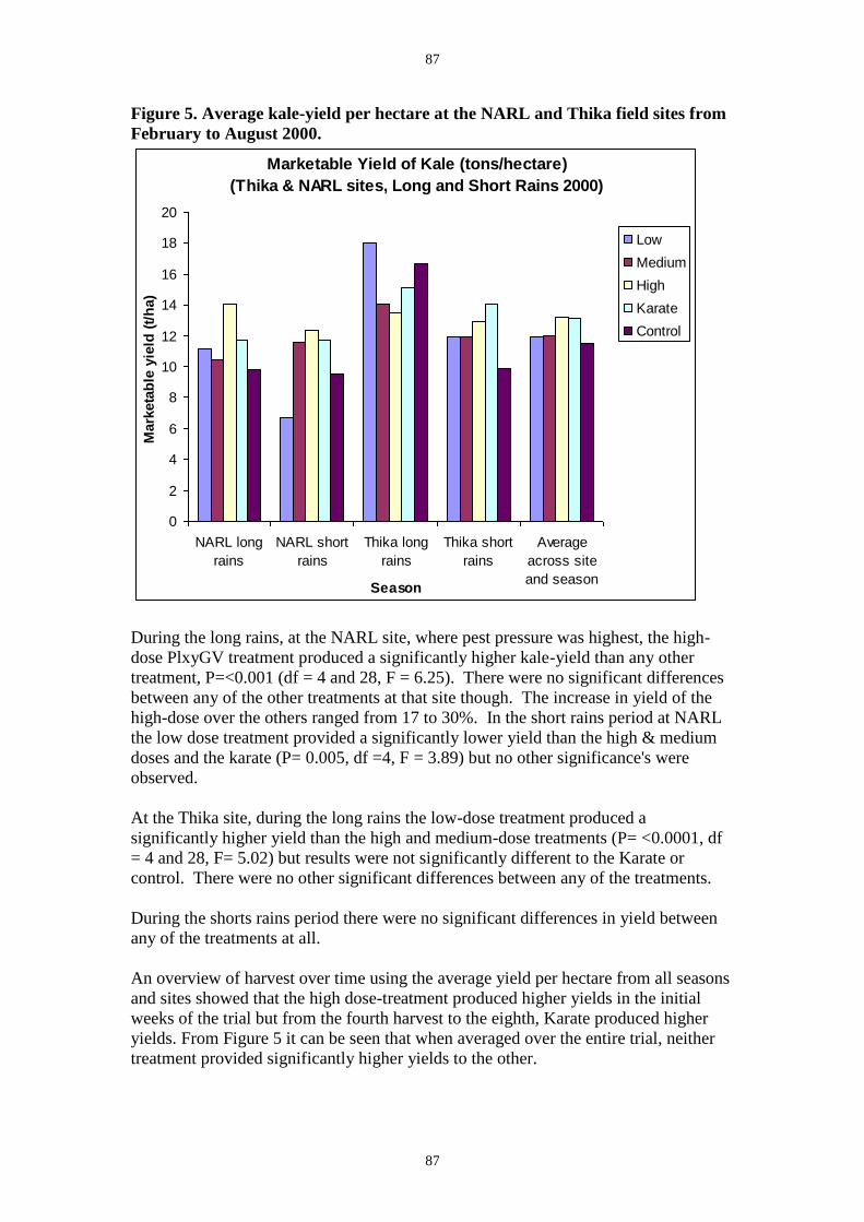
87

87

Figure 5. Average kale-yield per hectare at the NARL and Thika field sites from

February to August 2000.

During the long rains, at the NARL site, where pest pressure was highest, the high-

dose PlxyGV treatment produced a significantly higher kale-yield than any other

treatment, P=<0.001 (df = 4 and 28, F = 6.25). There were no significant differences

between any of the other treatments at that site though. The increase in yield of the

high-dose over the others ranged from 17 to 30%. In the short rains period at NARL

the low dose treatment provided a significantly lower yield than the high & medium

doses and the karate (P= 0.005, df =4, F = 3.89) but no other significance's were

observed.

At the Thika site, during the long rains the low-dose treatment produced a

significantly higher yield than the high and medium-dose treatments (P= <0.0001, df

= 4 and 28, F= 5.02) but results were not significantly different to the Karate or

control. There were no other significant differences between any of the treatments.

During the shorts rains period there were no significant differences in yield between

any of the treatments at all.

An overview of harvest over time using the average yield per hectare from all seasons

and sites showed that the high dose-treatment produced higher yields in the initial

weeks of the trial but from the fourth harvest to the eighth, Karate produced higher

yields. From Figure 5 it can be seen that when averaged over the entire trial, neither

treatment provided significantly higher yields to the other.

Marketable Yield of Kale (tons/hectare)


0

2

4

6

8

10

12

14

16

18

20

NARL long

rains

NARL short

rains

Thika long

rains

Thika short

rains

Average

across site

and seasonSeason

Mark

eta

ble

yie

ld (

t/h

a)

Low

Medium

High

Karate

Control

88

88

Figure 6. Average marketable yield from each treatment on each of the eight

harvests.

Observed infection rate

The mean infection rate of DBM populations overall ranged from 22.5% in the low

dose PlxyGV to 41.0% in the high dose PlxyGV. Maximum infection rate reached

100% and once infection had become established (by the third week) PlxyGV

symptoms were observed in every assessment. Figure 7 below shows the infection

rate over time for each of the treatments as an average taken from both seasons and

sites. It can be seen that as PlxyGV dose rate increased, so did the observed GV

infection rate (Figure 8). Analysis of data from the whole trial shows there were

significantly higher levels of infection in the medium and high dose than there were in

the low dose, (P= <0.001, df = 4, F = 94.9), but the difference in infection levels

between the medium and high-dose was not significant. The analysis also showed

levels of infection in the control and Karate were significantly lower than in all

PlxyGV treatments. Figure 8 shows that this trend was apparent at all levels of the

trial with dada from all sites and seasons showing the increase in infection level as

dose increased.

Marketable yield of Kale

(t/ha - summarised across site and season)

0.0

0.5

1.0

1.5

2.0

2.5

1 2 3 4 5 6 7 8 9

Observation week

Ma

rke

tab

le y

ield

(t/

ha

)

Low

Medium

High

Karate

Control

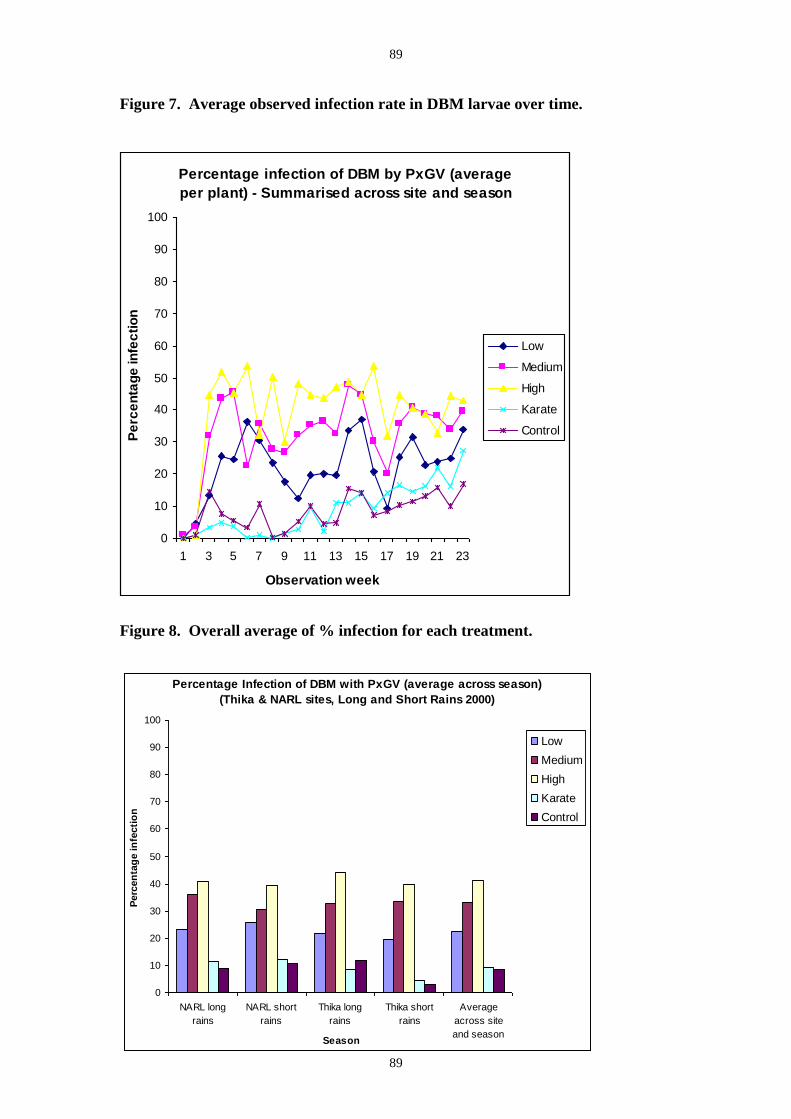
89

89

Figure 7. Average observed infection rate in DBM larvae over time.

Figure 8. Overall average of % infection for each treatment.

Percentage infection of DBM by PxGV (average

per plant) - Summarised across site and season

0

10

20

30

40

50

60

70

80

90

100

1 3 5 7 9 11 13 15 17 19 21 23

Observation week

Pe

rce

nta

ge

in

fec

tio

n

Low

Medium

High

Karate

Control

Percentage Infection of DBM with PxGV (average across season)


0

10

20

30

40

50

60

70

80

90

100

NARL long

rains

NARL short

rains

Thika long

rains

Thika short

rains

Average

across site

and seasonSeason

Perc

en

tag

e in

fecti

on

Low

Medium

High

Karate

Control

90

90

The independent experiment to compare levels of observed GV infection in he field at

any particular time to the final GV infection in observed larvae showed that larvae

from all instars collected succumbed to GV infection. In 4th instars the level of

infection reached a maximum of 60.6% infection (death) whereas in the 1st and 2

nd

instars, infection levels reached up to 90% (figure 9).

Figure 9. Infection levels in DBM larvae reared in the lab after being collected

from a virus-sprayed plot.

The infection rate in DBM larvae only appears to be density dependent for low dose

application. In this treatment, infection rate generally increased as the population

density grew (Figure 10), r2 =0.165.

Percent infection of different DBM larvae by PxGV applied in the field

0

10

20

30

40

50

60

70

80

90

100

Day 4 Day 7 Day 9

Time post-spray

% m

ort

ality

First Instar

Second instar

Third Instar

Fourth Instar

91

91

Figure 10. Density dependence of PlxyGV infection rate in low-dose treatments

of Kenyan field trials, February-August 2000.

In the medium and high-dose treatments, infection rate was not population density

dependant (Figures 11 and 12).

log10 total DBM population

103 104 105 106

% of DBM infected

-10

0

10

20

30

40

50

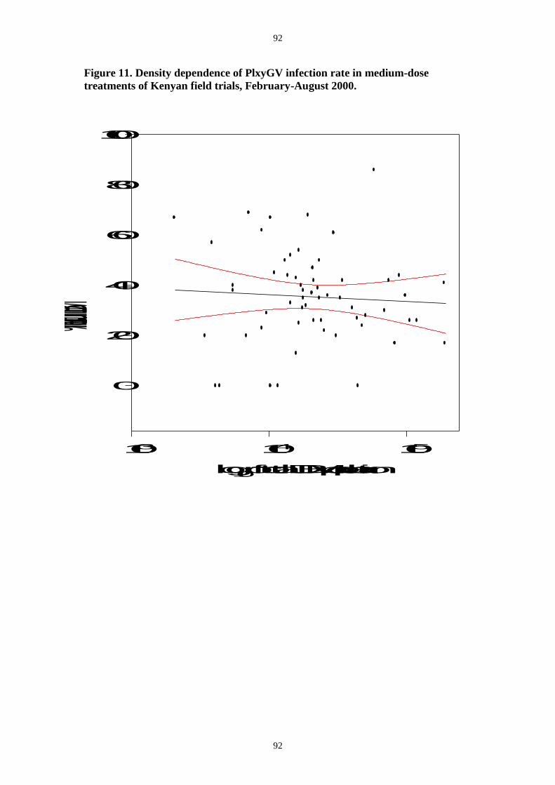
92

92

Figure 11. Density dependence of PlxyGV infection rate in medium-dose

treatments of Kenyan field trials, February-August 2000.

log10 of total DBM population

103 104 105

% infection in DBM

0

20

40

60

80

100

93

93

Figure 12. Density dependence of PlxyGV infection rate in high-dose treatments

of Kenyan field trials, February-August 2000.

Log10 total DBM population

103 104 105

% infected DBM

0

20

40

60

80

100

94

94

Discussion

Potency of PlxyGV field inoculum

The LC50 value of the field inoculum used in the current trial was not significantly

different to that of the inoculum used in the previous trial of 1998. Kenyan-based

local staff produced the batch used in the 2000 trial having previously received

training and the batch produced in 1998 was done under the supervision of an NRI

Insect Pathology expert. The inoculum of the previous trial had an LC50 value of 7.2

x106 OB/ml (Parnell, 1999) and that used here was 1.90 x10

7 OB/ml. Such

differences are within the normal variation seen in bioassays of baculovirus when

performed using the leaf-dip method and are often observed between replicates of the

same sample. Therefore the 2.6 fold difference in potency between two different

batches (samples) of PlxyGV is perfectly acceptable and is a good indication that the

PlxyGV production run was of high quality.

DBM Population

DBM populations were generally low throughout the season at both sites. This was

most marked at Thika where, on average, pest pressure was less than 1 larva per plant.

The highest population was recorded at only 2 larvae per plant and in many cases

(especially early on in the trial) no larvae at all were recorded. At NARL where pest

pressure was highest there were no more than 3 larvae per plant on average with a

maximum average population of 3.5 larvae per plant. Kenyan experts from KARI and

CABI-ARC expressed great surprise at such low infestation levels suggesting the

unusual rainfall patterns of two previous years may have been the cause.

The results obtained from the Karate treatment provide additional support to existing

evidence that this product causes significant increases in DBM populations on kale in

Kenya. The level of evidence is such that the Kenyan authorities are advising local

farmers against the use of Karate for DBM control and in farm visits made, it is

apparent that local farmers have begun to stop applying the current formulation of

Karate for DBM control already. As a trial average the Karate treatment caused

increases in DBM population of between 25 and 42%. All other treatments recorded

average populations per plant that were within 18% of each other indicating that the

known effect Karate has on reducing natural enemies may have been the cause of the

increase in those plots.

At the NARL site, difference in DBM population between treatments was more

pronounced than at Thika although the only significantly higher population was still

only observed in the Karate treatment. However a treatment effect was observed in

differences in DBM population between the control and PlxyGV doses and between

the different PlxyGV doses. The effect showed that even in exceptionally low

populations an increase in dose reduced the average DBM population. The only

occasion when this was not shown was in the long rains at Thika where, in general,

average DBM population per plant was less than 1 larva.

None of the PlxyGV treatments caused significantly lower DBM populations than the

control. It is likely that population levels were so low that a significant treatment

effect (other than for Karate) was undetectable given the size of plots used and the

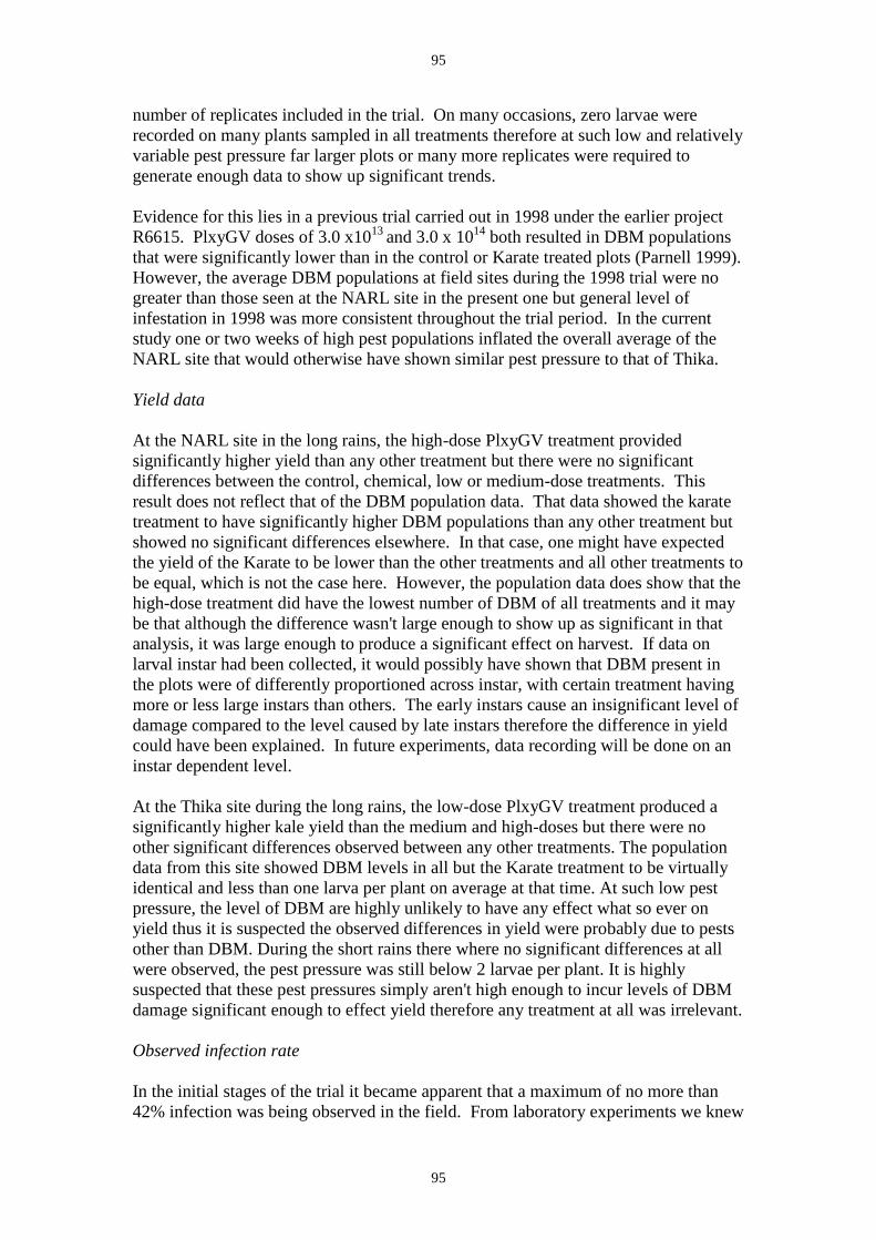
95

95

number of replicates included in the trial. On many occasions, zero larvae were

recorded on many plants sampled in all treatments therefore at such low and relatively

variable pest pressure far larger plots or many more replicates were required to

generate enough data to show up significant trends.

Evidence for this lies in a previous trial carried out in 1998 under the earlier project

R6615. PlxyGV doses of 3.0 x1013

and 3.0 x 1014

both resulted in DBM populations

that were significantly lower than in the control or Karate treated plots (Parnell 1999).

However, the average DBM populations at field sites during the 1998 trial were no

greater than those seen at the NARL site in the present one but general level of

infestation in 1998 was more consistent throughout the trial period. In the current

study one or two weeks of high pest populations inflated the overall average of the

NARL site that would otherwise have shown similar pest pressure to that of Thika.

Yield data

At the NARL site in the long rains, the high-dose PlxyGV treatment provided

significantly higher yield than any other treatment but there were no significant

differences between the control, chemical, low or medium-dose treatments. This

result does not reflect that of the DBM population data. That data showed the karate

treatment to have significantly higher DBM populations than any other treatment but

showed no significant differences elsewhere. In that case, one might have expected

the yield of the Karate to be lower than the other treatments and all other treatments to

be equal, which is not the case here. However, the population data does show that the

high-dose treatment did have the lowest number of DBM of all treatments and it may

be that although the difference wasn't large enough to show up as significant in that

analysis, it was large enough to produce a significant effect on harvest. If data on

larval instar had been collected, it would possibly have shown that DBM present in

the plots were of differently proportioned across instar, with certain treatment having

more or less large instars than others. The early instars cause an insignificant level of

damage compared to the level caused by late instars therefore the difference in yield

could have been explained. In future experiments, data recording will be done on an

instar dependent level.

At the Thika site during the long rains, the low-dose PlxyGV treatment produced a

significantly higher kale yield than the medium and high-doses but there were no

other significant differences observed between any other treatments. The population

data from this site showed DBM levels in all but the Karate treatment to be virtually

identical and less than one larva per plant on average at that time. At such low pest

pressure, the level of DBM are highly unlikely to have any effect what so ever on

yield thus it is suspected the observed differences in yield were probably due to pests

other than DBM. During the short rains there where no significant differences at all

were observed, the pest pressure was still below 2 larvae per plant. It is highly

suspected that these pest pressures simply aren't high enough to incur levels of DBM

damage significant enough to effect yield therefore any treatment at all was irrelevant.

Observed infection rate

In the initial stages of the trial it became apparent that a maximum of no more than

42% infection was being observed in the field. From laboratory experiments we knew

96

96

this was a very low infection rate so we conducted a small trial to ascertain if

observed infection rate on a single day of assessment was not a true indication of final

infection levels. The results showed that from initial infection rates of 0 to 28%

observed on what would have been a field assessment day, the final virus induced

mortality was between 60 and 90% depending on instar. The experiment was

replicated three times and a similar pattern emerged from each replicate leading to the

conclusion that an observed infection level of 40% on a single day in the field actually

represented up to a 90% infection level the generation of larvae present.

These results showed that infection rate in DBM larvae was only density dependant

when populations were treated with low-dose PlxyGV. It is the opinion of the

researchers that the increased infection rate with increased population was possibly

due to secondary cycling of PlxyGV released from larvae originally infected by the

applied dose. At medium and high-dose treatment where infection was not shown to

be density dependent, it is suspected that GV levels in the environment were such that

the effects of secondary infection were negligible, a marked increase in infection rate

was therefore not apparent.

Conclusion

From the results of this trial it is possible to say that at the low dose of 3.0x1012

OB/ha, control of DBM on kale would not be sufficient to make the application effort

worthwhile. It can also be said that it's highly likely that Karate is not able to control

DBM on kale and probably causes significant increases in population levels.

The pest pressure over all was uncharacteristically low compared to the last decade,

which confounded efforts to draw statistically valid conclusions. Where pest pressure

was highest the indication is that PlxyGV at the high dose of 3.0x1014

OB/ha would

provide significantly better control than any other treatment tested. However, at the

current time such an application rate would be uneconomically viable for DBM

control.

The work to follow on from these trials will be to investigate the effect of formulating

the PlxyGV to increase efficacy and thus lower the effective dose to an economically

viable application rate.

Reference

Matthews, G.A., (Ed) 1992. Pesticide Application Methods, 2nd Edition. Longman

Singapore Publishers Ltd., Singapore.

97

97

EVALUATION OF A NATURALLY OCCURRING BACULOVIRUS FOR THE

MANAGEMENT OF DIAMONDBACK MOTH, Plutella xylostella L. IN KENYA4

Walter Okello Ogutu1, George Isaiah Oduor

1, Mark Parnell

2, Douglas Waturu Miano

3,

Callistus K. P. O. Ogol4, Dave Grywacz

2, Jane Poole

1

1CAB International, Africa Regional Centre (CABI-ARC), P. O. Box 633-00621, Nairobi,

Kenya, 2Natural Resources Institute, The University of Greenwich, Central Avenue Chatham

Maritime, Kent ME4 4TB, UK, 3Kenya Agricultural Research Institute (KARI), P. O. Box

14733, Nairobi, Kenya 4Department of Zoology, Kenyatta University, P. O. Box 43844,

Nairobi, Kenya

Introduction

Diamondback moth (DBM) Plutella xylostella L. is a major pest of brassica crops in Kenya,

causing reduction in produce quality and yield. The most commonly practiced management

strategy for this pest in Kenya is the use of chemical insecticides. This use has generated

concerns regarding the cost, development of resistance to the most commonly used

insecticides, residues on produce and environmental contamination (Michalik, 1994, Kibata,

1997). A project to develop non-chemical methods of DBM control in Kenya has been

exploring the use of indigenous pathogens as potential control agents. Surveys in farmers‟

fields identified a baculovirus Plutella xylostella Granulovirus (PlxyGV) (Grzywacz et al.,

2002). Results from initial field trials indicated that PlxyGV was highly infectious to DBM

(Parnell, 1999). This paper reports on additional laboratory and field studies conducted at

Kabete and Thika, areas of contrasting ecologies close to Nairobi, with a view to

incorporating this naturally occurring baculovirus into a broader IPM package for DBM

management in Kenya.

4 Poster to be presented during the International Symposium – Improving Biocontrol of Plutella

xylostella, Montpellier, France, 21-24 October 2002.

98

98


Persistence of PlxyGV on potted cabbage plants

The virus used in the present study was produced using the protocols outlined by Parnell

(1999). A standard unpurified suspension of PlxyGV at a rate of 3.0 x 1013

OB/ ha was used

to spray 42 two-month-old plants, after which they were split into 6 groups of 7 plants.

Three groups were placed in three different shaded areas and three placed in open areas.

Once dry, one plant from each group was collected for immediate bioassay. The bioassay

was repeated on plants collected 7 hours, 1 day, 3, 7 and 9 days after spraying. At the time

of collection, fifteen 2nd

instar DBM larvae were placed on each plant. The larvae were

monitored daily until all had either died or developed to adulthood, and those showing virus

symptoms or death were recorded on the 4th, 7

th and 9

th day.

Evaluation of adjuvants to improve the efficacy of PlxyGV in the field

The effect of a combination of the most promising adjuvants (molasses and neem) on the

efficacy of PlxyGV against DBM larvae, assessed in laboratory studies (Grywacz D et al.,

2002), was evaluated in the field at Kabete and Thika. The unformulated PlxyGV,

formulated PlxyGV, Brigade® (Bifenthrin) and an unsprayed control were compared in

field plots of kale at two sites. Each treatment was replicated 6 times in a randomized

complete block (RCB) design in plots of sizes 4.2 x 3.6 m. A polythene sheet was used to

surround each plot during spraying time to act as a barrier against spray drift. Sampling was

done weekly on 10 randomly selected plants in each net plot. Numbers of pupae, larvae and

PlxyGV infected DBM, as well as damage caused by DBM were recorded. Yield data was

collected fortnightly by harvesting kale leaves in the net plot. After harvesting the leaves

were sorted into two groups, consisting of marketable and unmarketable leaves, (based on

grading criterion used by local farmers and also at the urban markets) and the numbers and

99

99

weights for each group recorded. These trials were conducted during the 2001 short rains

season (October 2001 – January 2002) and the 2002 long rains season (January –April).

Laboratory and field assessments of the effect of mixing PlxyGV with Pirimor®

The efficacy against DBM of the standard PlxyGV was compared to a mixture of standard

PlxyGV and Pirimor®, and an unsprayed control in the laboratory. The treatments were

prepared by thoroughly mixing the ingredients in a glass beaker. Twenty leaves of kale

were washed with moist cotton wool and left to dry. Five dry leaves were placed in each

test solution and left in the beaker for 1 hour. After drying, each leaf was placed in a round

plastic tub measuring 5cm in diameter and 7cm high and into each tub five 2nd

instar DBM

larvae were introduced. The larvae were monitored daily until all individuals had either

died or developed to adulthood. The number of larvae alive, infected and dead was

recorded on 4, 7 and 10 days after exposure. The efficacies of these same treatments were

also compared on field populations of DBM. Each treatment was replicated 4 times in a

RCB Design, each gross plot measuring 4.2 x 3.6 m. Observations were made as outlined

previously.

Effect of using a Conventional or V lance on the efficacy of PlxyGV against DBM

The efficacy of PlxyGV using a conventional and V lance was investigated in field trial

plots at two sites. For comparison a treatments using both lances and a chemical insecticide,

fipronil (Regent®), and an untreated control were included. The trial consisted of 5

treatments, PlxyGV standard dose and fipronil sprayed using either the conventional or V

lance and untreated control. Each treatment was replicated four times in a RCB Design,

each gross plot measuring 4.2 x 3.6 m. The trials were conducted over two growing

seasons, the 2001 long rains and short rains respectively. Observations were made as

outlined previously.

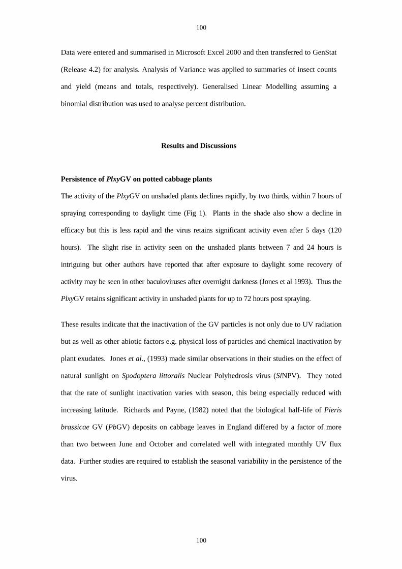
100

100

Data were entered and summarised in Microsoft Excel 2000 and then transferred to GenStat

(Release 4.2) for analysis. Analysis of Variance was applied to summaries of insect counts

and yield (means and totals, respectively). Generalised Linear Modelling assuming a

binomial distribution was used to analyse percent distribution.

Results and Discussions

Persistence of PlxyGV on potted cabbage plants

The activity of the PlxyGV on unshaded plants declines rapidly, by two thirds, within 7 hours of

spraying corresponding to daylight time (Fig 1). Plants in the shade also show a decline in

efficacy but this is less rapid and the virus retains significant activity even after 5 days (120

hours). The slight rise in activity seen on the unshaded plants between 7 and 24 hours is

intriguing but other authors have reported that after exposure to daylight some recovery of

activity may be seen in other baculoviruses after overnight darkness (Jones et al 1993). Thus the

PlxyGV retains significant activity in unshaded plants for up to 72 hours post spraying.

These results indicate that the inactivation of the GV particles is not only due to UV radiation

but as well as other abiotic factors e.g. physical loss of particles and chemical inactivation by

plant exudates. Jones et al., (1993) made similar observations in their studies on the effect of

natural sunlight on Spodoptera littoralis Nuclear Polyhedrosis virus (SlNPV). They noted

that the rate of sunlight inactivation varies with season, this being especially reduced with

increasing latitude. Richards and Payne, (1982) noted that the biological half-life of Pieris

brassicae GV (PbGV) deposits on cabbage leaves in England differed by a factor of more

than two between June and October and correlated well with integrated monthly UV flux

data. Further studies are required to establish the seasonal variability in the persistence of the

virus.

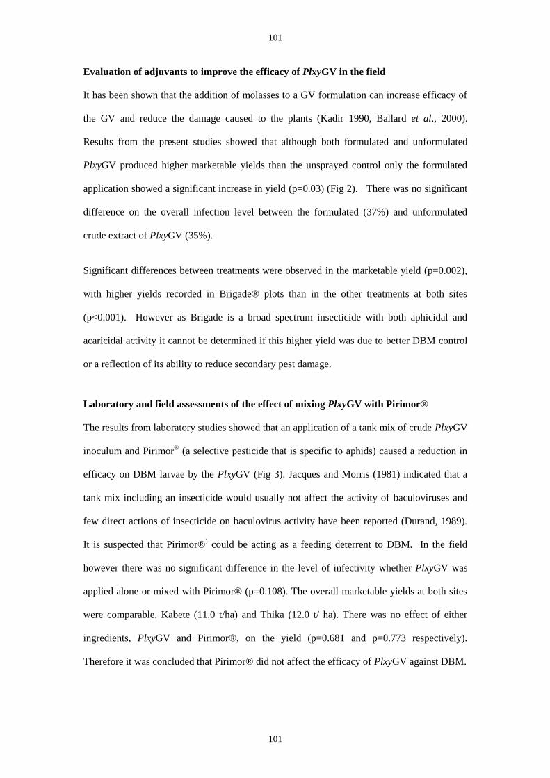
101

101

Evaluation of adjuvants to improve the efficacy of PlxyGV in the field

It has been shown that the addition of molasses to a GV formulation can increase efficacy of

the GV and reduce the damage caused to the plants (Kadir 1990, Ballard et al., 2000).

Results from the present studies showed that although both formulated and unformulated

PlxyGV produced higher marketable yields than the unsprayed control only the formulated

application showed a significant increase in yield (p=0.03) (Fig 2). There was no significant

difference on the overall infection level between the formulated (37%) and unformulated

crude extract of PlxyGV (35%).

Significant differences between treatments were observed in the marketable yield (p=0.002),

with higher yields recorded in Brigade® plots than in the other treatments at both sites

(p<0.001). However as Brigade is a broad spectrum insecticide with both aphicidal and

acaricidal activity it cannot be determined if this higher yield was due to better DBM control

or a reflection of its ability to reduce secondary pest damage.

Laboratory and field assessments of the effect of mixing PlxyGV with Pirimor®

The results from laboratory studies showed that an application of a tank mix of crude PlxyGV

inoculum and Pirimor® (a selective pesticide that is specific to aphids) caused a reduction in

efficacy on DBM larvae by the PlxyGV (Fig 3). Jacques and Morris (1981) indicated that a

tank mix including an insecticide would usually not affect the activity of baculoviruses and

few direct actions of insecticide on baculovirus activity have been reported (Durand, 1989).

It is suspected that Pirimor®) could be acting as a feeding deterrent to DBM. In the field

however there was no significant difference in the level of infectivity whether PlxyGV was

applied alone or mixed with Pirimor® (p=0.108). The overall marketable yields at both sites

were comparable, Kabete (11.0 t/ha) and Thika (12.0 t/ ha). There was no effect of either

ingredients, PlxyGV and Pirimor®, on the yield (p=0.681 and p=0.773 respectively).

Therefore it was concluded that Pirimor® did not affect the efficacy of PlxyGV against DBM.

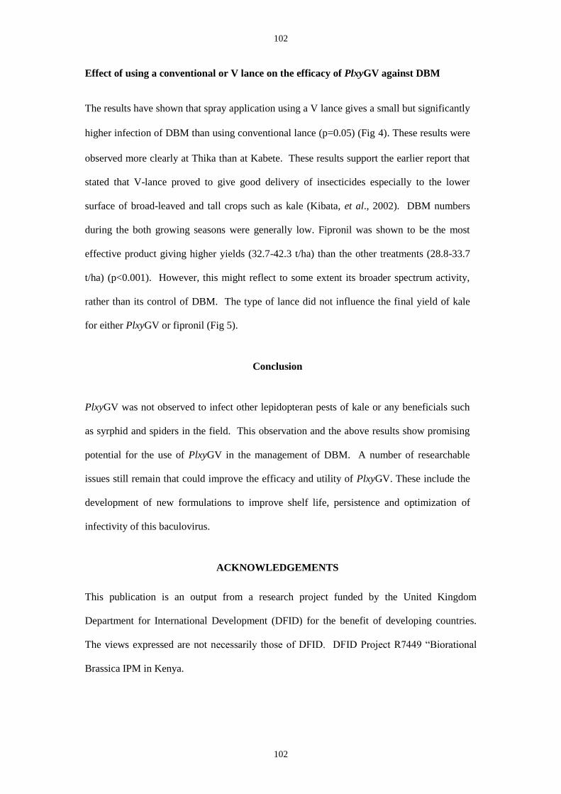
102

102

Effect of using a conventional or V lance on the efficacy of PlxyGV against DBM

The results have shown that spray application using a V lance gives a small but significantly

higher infection of DBM than using conventional lance (p=0.05) (Fig 4). These results were

observed more clearly at Thika than at Kabete. These results support the earlier report that

stated that V-lance proved to give good delivery of insecticides especially to the lower

surface of broad-leaved and tall crops such as kale (Kibata, et al., 2002). DBM numbers

during the both growing seasons were generally low. Fipronil was shown to be the most

effective product giving higher yields (32.7-42.3 t/ha) than the other treatments (28.8-33.7

t/ha) (p<0.001). However, this might reflect to some extent its broader spectrum activity,

rather than its control of DBM. The type of lance did not influence the final yield of kale

for either PlxyGV or fipronil (Fig 5).

Conclusion

PlxyGV was not observed to infect other lepidopteran pests of kale or any beneficials such

as syrphid and spiders in the field. This observation and the above results show promising

potential for the use of PlxyGV in the management of DBM. A number of researchable

issues still remain that could improve the efficacy and utility of PlxyGV. These include the

development of new formulations to improve shelf life, persistence and optimization of

infectivity of this baculovirus.

ACKNOWLEDGEMENTS

This publication is an output from a research project funded by the United Kingdom

Department for International Development (DFID) for the benefit of developing countries.

The views expressed are not necessarily those of DFID. DFID Project R7449 “Biorational

Brassica IPM in Kenya.

103

103

REFERENCES

Abdul-Kadir, H. B., (1990). Potential of several baculoviruses for the control of

diamondback moth and Croccidolomia binotalis on cabbages. In: “Diamondback

moth and other crucifer pets”, proceedings of the 2nd

International Workshop,

Tainan, Taiwan, 10-14 December 1990, N. S. Talekar, (ed) 185-192.

Ballard, D. J. Ellis and Payne, C.C., (2000). The role of Additives in Increasing the Potency

of Cydia pomonella Granulovirus for Codling Moth Larvae, in Laboratory and Field

Experiments. In Biocontrol Science and Technology (2002) 10, 627-640.

Durand, N., (1989). Study on the Control of Diamondback moth Plutella xylostella (Linnẽ)

(Lep.: Hyponomeutidae) using Mametra brassicae Nuclear Polyhedrosis virus and

it‟s combination with a synthetic pyrethroids. Pp40

Entwistle, P.F. and Evans, H.F., (1985) Viral control. In Comprehensive Insect Physiology,

Biochemistry and Pharmacology, Vol. 12. Oxford: Pergamon Press, pp. 347-412.

Grzywacz, D., Parnell, M, Kibata, G., Oduor G., Ogutu.

W.O., Poole, J., and Miano, D.,

(2002). The granulovirus of Plutella xylostella (diamond back moth DBM) and its

potential for control of DBM in Kenya. International symposium improving

biocontrol of Plutella xylostella. 21-24th October 2002, Montpellier, France, pp6.

Jacques, R. P. and O. N. Morris. 1981. Compatibility of pathogens with other methods of

pest control and crop protection. In Microbial Control of Pests and Plant Diseases,

Burges, H. D. [ed.] Academic Press, London UK.

Jones, K. A., Moawad, G. Mckinley, D.J., and Grzywacz, D., (1993). The effect of Natural

sunlight on Spodoptera littoralis Nuclear Polyhedrosis Virus. Biocontrol Science and

Technology 3, 189-197.

104

104

Kibata, G.N., (1997). The Diamondback moth: A problem pest of brassica crops in Kenya.

In “Sivapragasam, A., Loke, W.H., Kadir, A.H., Lim, G.S., (eds). The Management

of

Diamondback Moth and Other Crucifer Pests. Proceedings of the 3rd

International

Workshop, Kuala Lumpur, Malaysia 29 October – 1 November 1996, MARDI,

Malaysia, pp 47-53.

Kibata G.N., Cooper, J., and Oduor G. (2002) Better Targeting of Sprays. In Horticultural

News, Horticultural Crops Development Authority (HCDA). No. 26 January /

February, 2002 Issue.

Parnell, M., (1999). The genetic variability and efficacy of baculoviruses for the control of

Diamondback moth on brassica vegetables in Kenya. M.Sc Research Thesis, The

Natural Resources Institute, University of Greenwich, UK

Michalik, S., (1994). Report on crop protection measures of Kenyan vegetable farmers and

their use of pesticides: A knowledge, attitude and practical survey. KARI/GTZ IPM

Horticulture Project.

Richards, M. G. and Payne, C.C., (1982) Persistence of baculovirus on leaf surfaces. In

Proceedings of the 3rd

International Colloquium on Invertebrate Pathology. Brighton.

Pp. 296-301

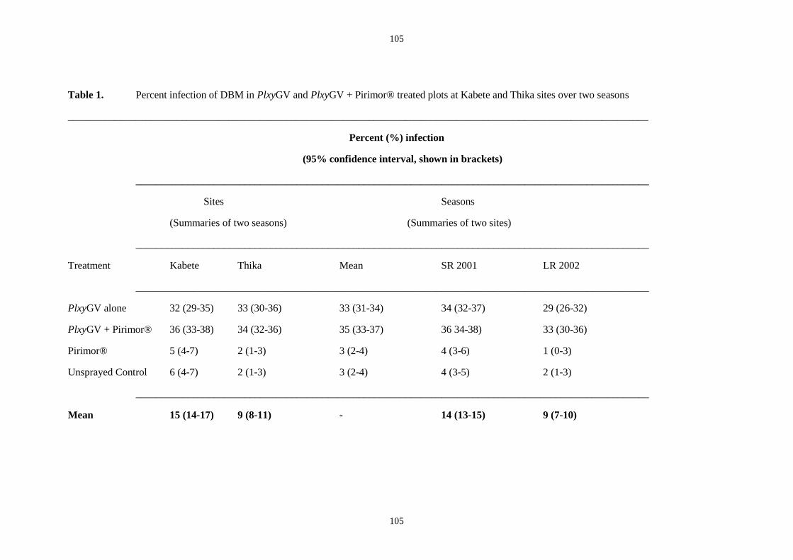
105

105

Table 1. Percent infection of DBM in PlxyGV and PlxyGV + Pirimor® treated plots at Kabete and Thika sites over two seasons

________________________________________________________________________________________________________________

Percent (%) infection

(95% confidence interval, shown in brackets)

___________________________________________________________________________________________________

Sites Seasons

(Summaries of two seasons) (Summaries of two sites)

___________________________________________________________________________________________________

Treatment Kabete Thika Mean SR 2001 LR 2002

___________________________________________________________________________________________________

PlxyGV alone 32 (29-35) 33 (30-36) 33 (31-34) 34 (32-37) 29 (26-32)

PlxyGV + Pirimor® 36 (33-38)

34 (32-36) 35 (33-37) 36 34-38) 33 (30-36)

Pirimor®

5 (4-7) 2 (1-3) 3 (2-4) 4 (3-6) 1 (0-3)

Unsprayed Control 6 (4-7) 2 (1-3) 3 (2-4) 4 (3-5) 2 (1-3)

___________________________________________________________________________________________________

Mean 15 (14-17) 9 (8-11) - 14 (13-15) 9 (7-10)

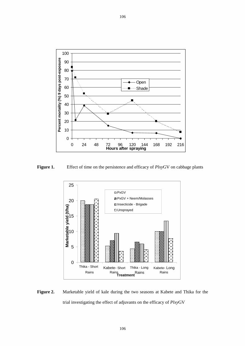
106

106

Figure 1. Effect of time on the persistence and efficacy of PlxyGV on cabbage plants

Figure 2. Marketable yield of kale during the two seasons at Kabete and Thika for the

trial investigating the effect of adjuvants on the efficacy of PlxyGV

0

10

20

30

40

50

60

70

80

90

100

0 24 48 72 96 120 144 168 192 216Hours after spraying

Perc

en

t m

ort

ality

(%

) 9 d

ays p

ost-

exp

osu

re

Open

Shade

0

5

10

15

20

25

Thika - Short

Rains Kabete- Short

Rains Thika - Long

Rains

Kabete- Long Rains

Treatment

Mark

eta

ble

yie

ld (

t/h

a)

PxGV

PxGV + Neem/Molasses

Insecticide - Brigade

Unsprayed

107

107

Figure 3. Effect of mixing PlxyGV with Pirimor® in the laboratory

Figure 4. Overall percent infection level of DBM in treated plots using V-lance and

conventional lance at the two sites over the two seasons

0

10

20

30

40

50

60

70

80

90

100

PxGV & Pirimor PxGV alone Treatment

Perc

en

t in

fecti

on

4days post-exposure

7days post-exposure

9days post-exposure

0

10

20

30

40

50

60

70

80

90

100

1 2 3 4 5 6 7 8 9 10 11 12 13 14 15Week

% I

nfe

cti

on

PxGV (C-L)

Fipronil (C-L)

PxGV (V-L)

Fipronil (V-L)

Unsprayed

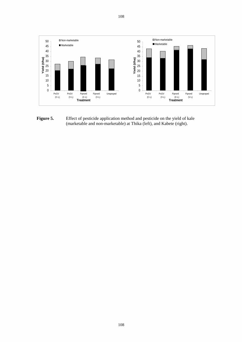
108

108

Figure 5. Effect of pesticide application method and pesticide on the yield of kale

(marketable and non-marketable) at Thika (left), and Kabete (right).

0 5

10 15 20 25 30 35 40 45 50

PxGV (C-L)

PxGV (V-L)

Fipronil (C-L)

Fipronil (V-L)

Unsprayed

Treatment

Yie

ld (

t/h

a)

Non-marketable Marketable

0 5

10 15 20 25 30 35 40 45 50

PxGV (C-L)

PxGV (V-L)

Fipronil (C-L)

Fipronil (V-L)

Unsprayed

Treatment

Yie

ld (

t/h

a)

Non-marketable Marketable

109

109

The granulovirus of Plutella xylostella (diamond back moth ,DBM) and its potential for

control of DBM in Kenya.

David Grzywacz1, Mark Parnell

1, Gilbert Kibata

2, George Oduor

3, Jane Poole

3, Walter

Ogutu3 and Douglas Miano

2.

1: Sustainable Agriculture Group, Natural Resources Institute, University of Greenwich, Central

Avenue, Chatham Maritime, Kent ME4 4TB, UK.


3: CAB International, Africa Regional Centre, PO Box 633, Village Market, Nairobi, Kenya.

Introduction

DBM is a major pest of brassica vegetables in Kenya (Michalik 1994). In East Africa, control of

DBM is becoming an increasing problem due to escalating resistance to chemical insecticides. A

project to develop non-chemical methods of DBM control on brassica crops was initiated in

Kenya in 1996 to explore the use of endemic pathogens for DBM control. Prior to this study

granuloviruses (GV) of P.xylostella had been reported from Japan (Asayama and Osaki 1970)

Taiwan and China (Kadir et al 1999) and India (Rabindra et al, 1997), but there were no previous

published records of PlxyGV isolates from Africa.


A survey of 27 brassica farms was conducted within a radius of 170 km around Nairobi to

identify endemic pathogens of DBM. Larvae showing signs of baculovirus infection, were

collected for later examination and the presence of GV confirmed. Restriction endonuclease

analysis (REN) of the baculovirus isolates was performed on each of the GV isolates found,

following the protocol of Smith and Summers (1978). The pathogenicity of eight of the

fourteen isolates showing different REN profiles were determined by discriminate dose

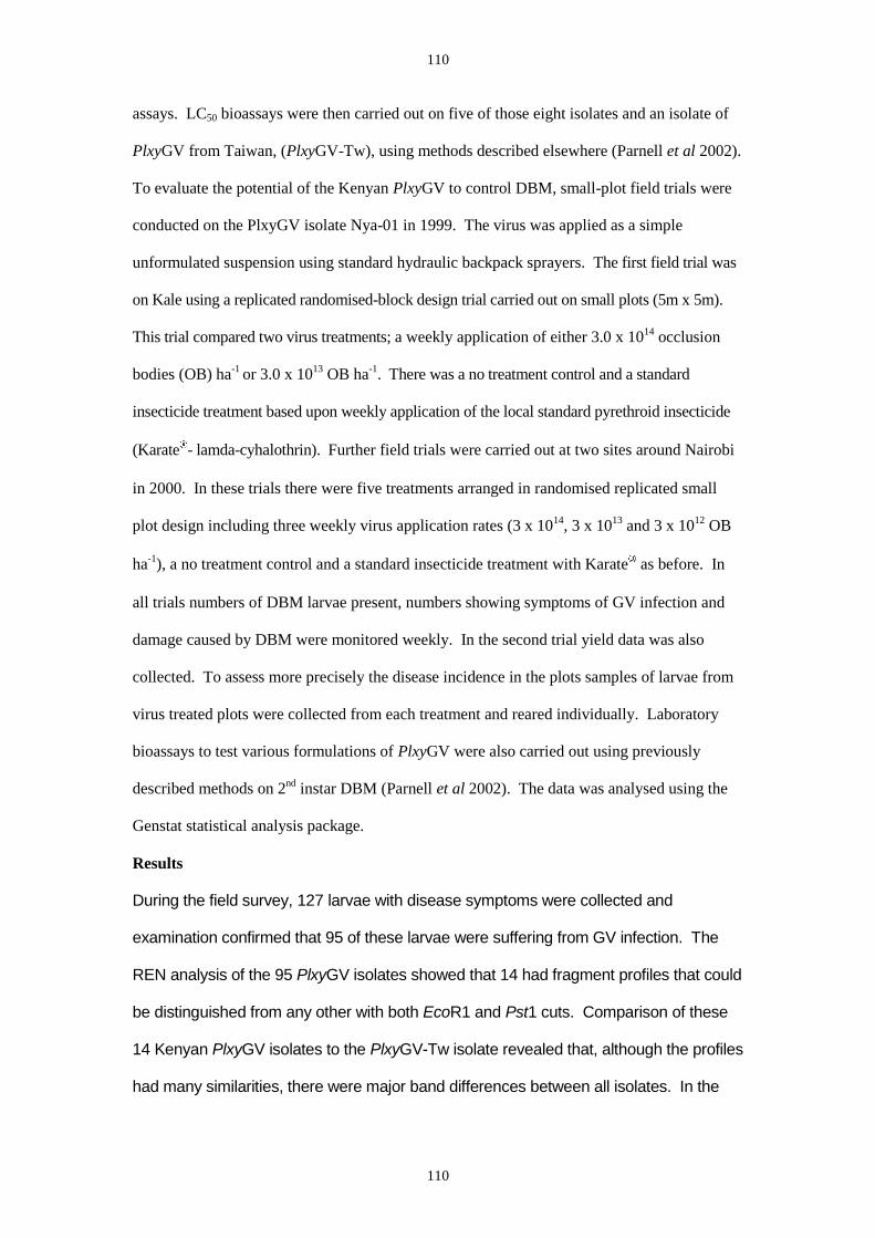
110

110

assays. LC50 bioassays were then carried out on five of those eight isolates and an isolate of

PlxyGV from Taiwan, (PlxyGV-Tw), using methods described elsewhere (Parnell et al 2002).

To evaluate the potential of the Kenyan PlxyGV to control DBM, small-plot field trials were

conducted on the PlxyGV isolate Nya-01 in 1999. The virus was applied as a simple

unformulated suspension using standard hydraulic backpack sprayers. The first field trial was

on Kale using a replicated randomised-block design trial carried out on small plots (5m x 5m).

This trial compared two virus treatments; a weekly application of either 3.0 x 1014

occlusion

bodies (OB) ha-1

or 3.0 x 1013

OB ha-1

. There was a no treatment control and a standard

insecticide treatment based upon weekly application of the local standard pyrethroid insecticide

(Karate - lamda-cyhalothrin). Further field trials were carried out at two sites around Nairobi

in 2000. In these trials there were five treatments arranged in randomised replicated small

plot design including three weekly virus application rates (3 x 1014

, 3 x 1013

and 3 x 1012

OB

ha-1

), a no treatment control and a standard insecticide treatment with Karate as before. In

all trials numbers of DBM larvae present, numbers showing symptoms of GV infection and

damage caused by DBM were monitored weekly. In the second trial yield data was also

collected. To assess more precisely the disease incidence in the plots samples of larvae from

virus treated plots were collected from each treatment and reared individually. Laboratory

bioassays to test various formulations of PlxyGV were also carried out using previously

described methods on 2nd

instar DBM (Parnell et al 2002). The data was analysed using the

Genstat statistical analysis package.

Results

During the field survey, 127 larvae with disease symptoms were collected and

examination confirmed that 95 of these larvae were suffering from GV infection. The

REN analysis of the 95 PlxyGV isolates showed that 14 had fragment profiles that could

be distinguished from any other with both EcoR1 and Pst1 cuts. Comparison of these

14 Kenyan PlxyGV isolates to the PlxyGV-Tw isolate revealed that, although the profiles

had many similarities, there were major band differences between all isolates. In the

111

111

dose response bioassays no significant differences in LC50 values between Kenyan

isolates and the PlxyGV-Tw isolate were observed. Average LC50 values for second

instar DBM larvae ranged from 2.36x106 OB ml-1 for Nya-01 to 3.95x107 OB ml-1 for

isolate Nya-40. In comparison the LC50 for the PlxyGV-Tw was 1.55x107 OB ml-1.

Bioassays of simple formulations of PlxyGV showed the LC50 for the formulated virus to

be 3.62 x105 OB ml-1 compared to 3.65 x107 OB ml-1 with the unformulated control. The

productivity study showed that the maximum production of PlxyGV was 4.0 0.44 x1010

OB per larva from 2nd instars inoculated with 2 x108 OB ml-1.

The field trials showed that the PlxyGV was highly infectious to DBM, spreading rapidly

in trial plots within two to three weeks of application. Both the high application rate of

3.0 x 1014 OB ha-1and the lower application rate of 3.0 x 1013 OB ha-1 reduced DBM

damage to crops to below that seen in either unsprayed controls or insecticide treated

plots (Figure 1). In the second series of trials the yield data (Figure 2) showed that the

highest application rate of virus gave a mean yield 37% higher than the control and 17%

higher than the insecticide treatment, although this was not statistically significant. The

average observed DBM infection rates in virus treated plots also showed a clear

application-rate trend with the highest rate producing an average of 40% infection in

DBM larvae (Figure 3). A study of insects sampled from the PlxyGV application-rate

plots indicated that the true infection rate was much higher than that observed in the

field and Table 1 shows the percent virus mortality recorded from insects taken from the

plot treated at 3 x1013 OB ha-1.

Discussion

The discovery of numerous genetic isolates (14) in the small number of infected larvae

collected is an interesting result. Previously reported work (Kadir et al 1999) has

characterised two genetically distinct isolates, one from China and one from Taiwan. Other

studies of DBM pathogens have also only reported finding a single genetically distinct isolate

from India (Rabindra et al 1997) and Japan (Yamada & Yamaguchi 1985). The GV isolates

112

112

from Kenya are genetically similar to, though distinct from the previously reported Taiwanese

isolate. The genetic variation in PlxyGV isolates discovered in Kenya might indicate a long

relationship between host and virus and could be interpreted as providing additional support

to the theory of Kfir (1998) that the origin of DBM lies in Sub-Saharan Africa.

The first field trial showed that application of PlxyGV at 3x1013

OB ha-1

could reduce DBM

damage much better than Karate the standard chemical insecticide. In the second trial the

yield results showed that again the PlxyGV performed as well as the chemical insecticide at

the highest application rate used (3x1014

OB ha-1

). The lower application rates did not result

in effective DBM control. The yield data for the PlxyGV at 3x1014

OB ha-1

, while higher was

not significantly better than the insecticide. This may be because PlxyGV does not control

aphids while the chemical insecticide does. In many seasons Kenya aphids are a serious

secondary pests of brassicas (Oruko and Ndun‟gu 2001) and if PlxyGv is to be successfully

promoted to farmers there will be a need to identify an effective compatible aphid control.

system.

The productivity of the Kenyan isolates is high at 2.0-4.0 0.44 x1010

OB per larva. At this

rate of production the highest application rate used in the field trials, 3.0 x1014

OB ha-1

would

be equivalent to 7,500 infected larvae per ha. In comparison most existing commercial

baculovirus products are applied at rates of between 50-500 larval equivalents per ha

(Moscardi 1999). The two granuloviruses that have been commercialised to date, Cydia

pomonella GV and Adoxophyes orana GV, both have application at rates of 1x1013

OB ha-1

.

Thus an an application rate of 3.0 x1014

OB ha-1

could be higher than is economically viable.

It has been shown that the addition of molasses to a GV formulation can increase the efficacy

of the GV by a factor of ten, and allow for a consequent reduction in the application rate of

(Kadir 1992, Ballard et al 2000). Laboratory bioassays showed that a molasses formulation

of PlxyGV indeed reduces the LC50 by a factor of 50. Thus formulation could significantly

lower the potential cost of PlxyGV. Successful field trials of such a formulation have recently

113

113

been completed in Kenya to evaluate the efficacy of reduced rate formulated PlxyGV and are

reported elsewhere at this meeting (Ogutu et al 2002).

In conclusion, from the results of these trials it may be concluded that PlxyGV has

considerable potential as a biopesticide for controlling DBM, and further work to evaluate its

potential commercial use in Kenya is now underway.

This publication is an output from a research project funded by the United Kingdom

Department for International Development (DFID) for the benefit of developing

countries. The views expressed are not necessarily those of DFID. DFID Project

R7449 “Biorational Brassica IPM in Kenya.

References

Abdul Kadir, H.B. (1992). Potential of several baculoviruses for the control of diamondback

moth and Crocidolomia binotalis on cabbages. In: Talekar, N.S. (Ed), "Diamondback Moth

and Other Crucifer Pests." Proceedings of the Second International Workshop, Tainan,


Abdul Kadir, H.B., Payne, C.C., Crook, N.E., and Winstanley, D. (1999). Characterization

and cross-transmission of baculoviruses infective to the diamondback moth, Plutella

xylostella, and some other Lepidopterous pests of brassica crops. Biocontrol Science and

Technology 9, 227-238.

Asayama, T. and Osaki, N. (1970). A granulosis of the diamondback moth, Plutella


Ballard, J., Ellis, D. J. and Payne, C. C. (2000). The role of formulation additives in

increasing the potency of Cydia pomonella granulovirus for coddling moth larvae in

laboratory and field experiments. Biocontrol Science and Technology 10:627-640.

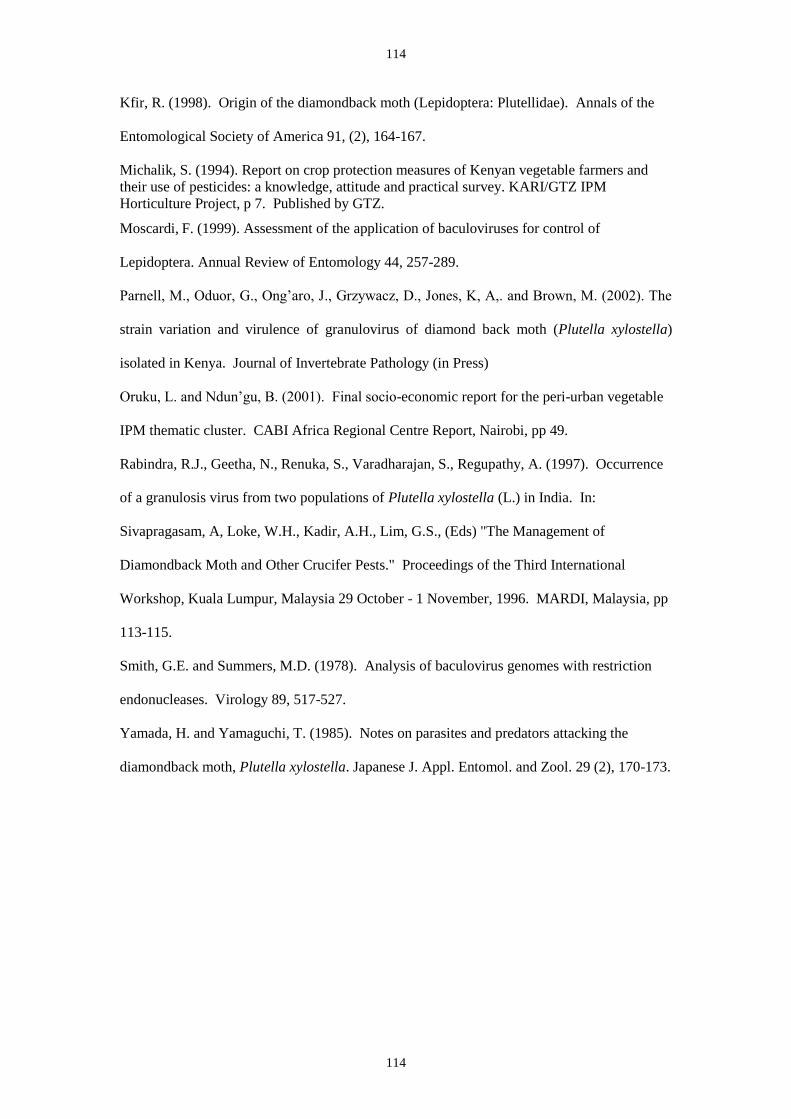
114

114

Kfir, R. (1998). Origin of the diamondback moth (Lepidoptera: Plutellidae). Annals of the

Entomological Society of America 91, (2), 164-167.

Michalik, S. (1994). Report on crop protection measures of Kenyan vegetable farmers and



Moscardi, F. (1999). Assessment of the application of baculoviruses for control of

Lepidoptera. Annual Review of Entomology 44, 257-289.

Parnell, M., Oduor, G., Ong‟aro, J., Grzywacz, D., Jones, K, A,. and Brown, M. (2002). The

strain variation and virulence of granulovirus of diamond back moth (Plutella xylostella)

isolated in Kenya. Journal of Invertebrate Pathology (in Press)

Oruku, L. and Ndun‟gu, B. (2001). Final socio-economic report for the peri-urban vegetable

IPM thematic cluster. CABI Africa Regional Centre Report, Nairobi, pp 49.

Rabindra, R.J., Geetha, N., Renuka, S., Varadharajan, S., Regupathy, A. (1997). Occurrence

of a granulosis virus from two populations of Plutella xylostella (L.) in India. In:

Sivapragasam, A, Loke, W.H., Kadir, A.H., Lim, G.S., (Eds) "The Management of

Diamondback Moth and Other Crucifer Pests." Proceedings of the Third International


113-115.

Smith, G.E. and Summers, M.D. (1978). Analysis of baculovirus genomes with restriction


Yamada, H. and Yamaguchi, T. (1985). Notes on parasites and predators attacking the

diamondback moth, Plutella xylostella. Japanese J. Appl. Entomol. and Zool. 29 (2), 170-173.

115

115

Table 1. Percentage insects killed by PlxyGV infections that developed in laboratory

reared larvae sampled from field plots sprayed with PlxyGV at 3x1013

OB ha-1

.

Larval instar % PlxyGV mortality

1st Instar 90

2nd

Instar 82

3rd

Instar 64

4th Instar 60

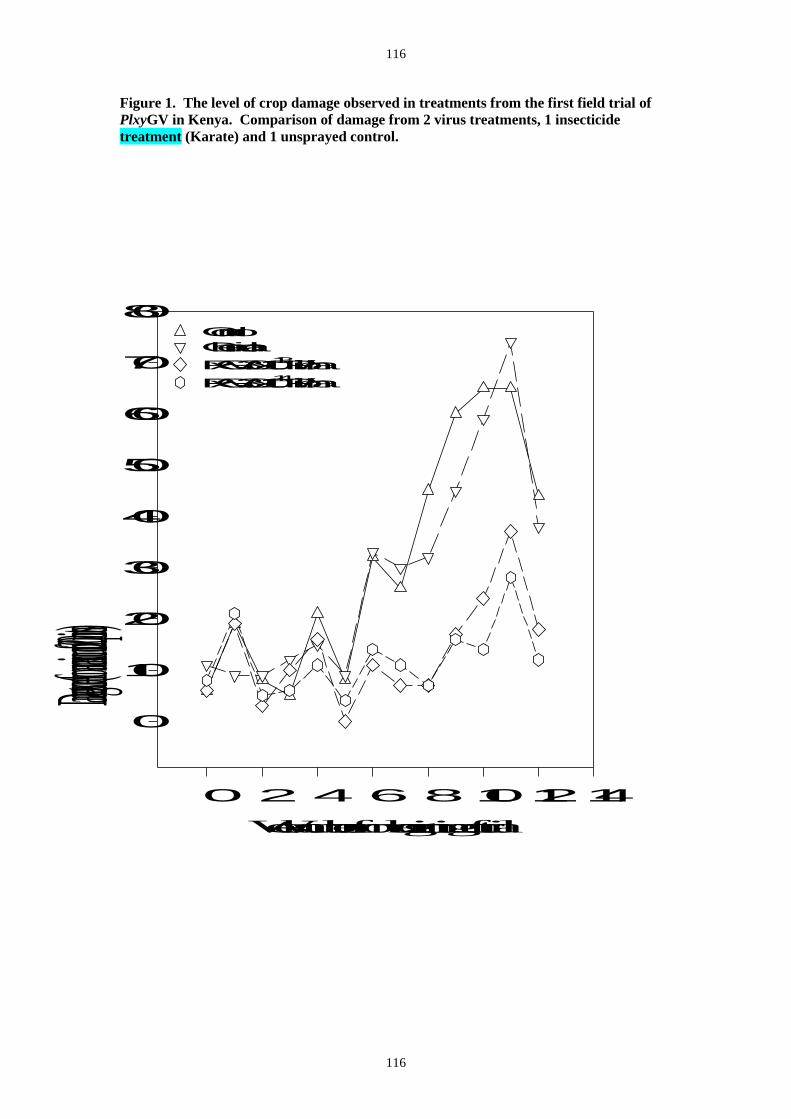
116

116

Figure 1. The level of crop damage observed in treatments from the first field trial of

PlxyGV in Kenya. Comparison of damage from 2 virus treatments, 1 insecticide

treatment (Karate) and 1 unsprayed control.

Week number from beginning of trial

0 2 4 6 8101214

Damage score (from a maximumof 200 po

ints)

0

10

20

30

40

50

60

70

80Control

Chemical

PxGV 3.0x1013 Pib/ha

PxGV 3.0x1014 Pib/ha

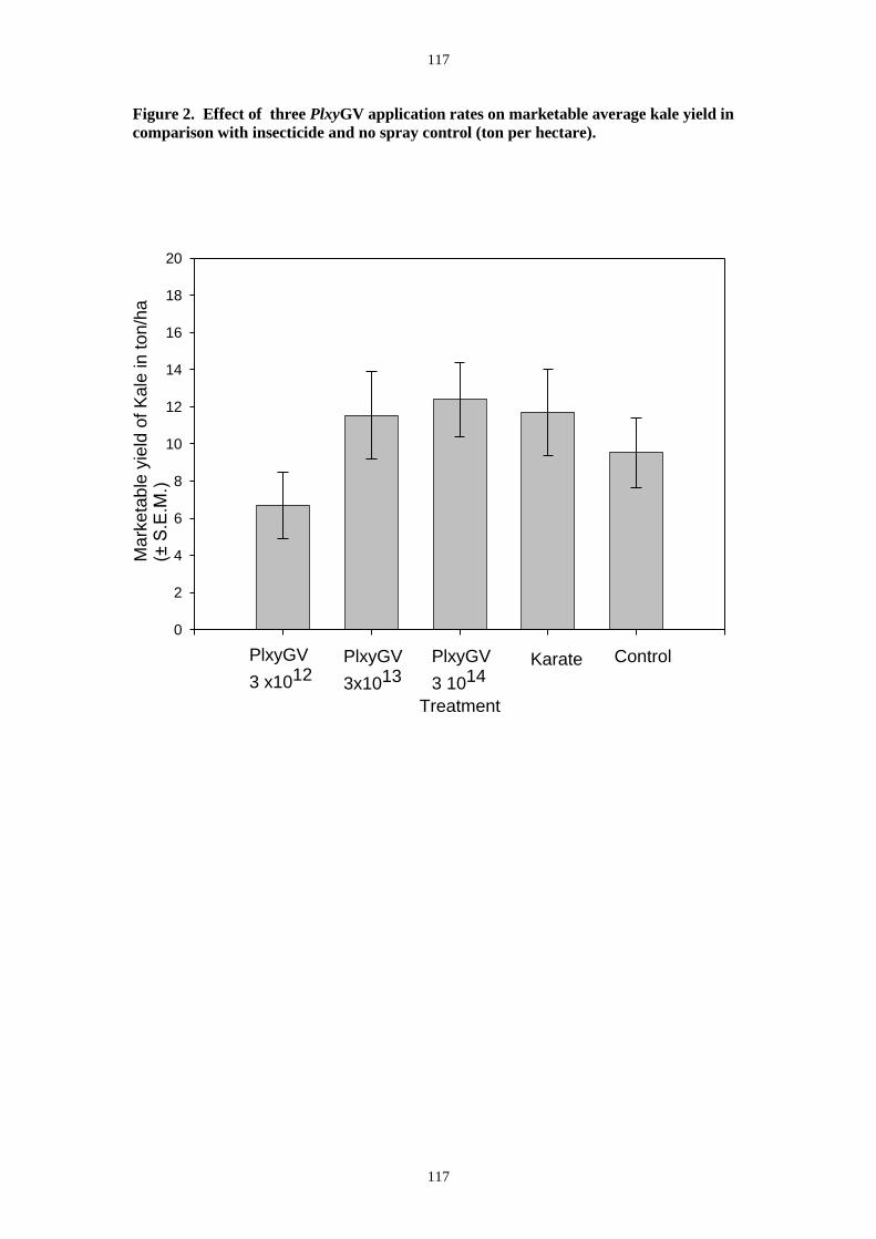
117

117

Figure 2. Effect of three PlxyGV application rates on marketable average kale yield in

comparison with insecticide and no spray control (ton per hectare).

Treatment

Mark

eta

ble

yie

ld o

f K

ale

in ton/h

a

(± S

.E.M

.)

0

2

4

6

8

10

12

14

16

18

20

PlxyGV

3 x1012PlxyGV

3x1013

PlxyGV

3 1014Karate Control

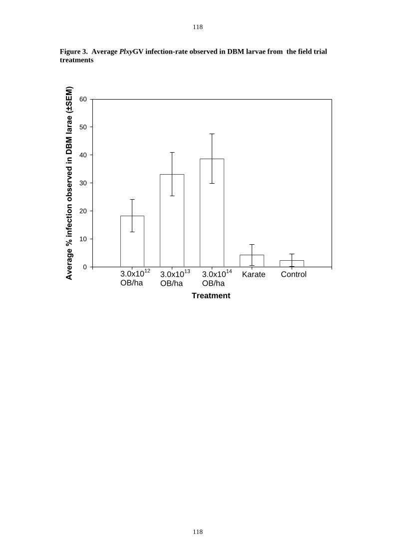
118

118

Figure 3. Average PlxyGV infection-rate observed in DBM larvae from the field trial

treatments

Treatment

Avera

ge %

in

fecti

on

ob

serv

ed

in

DB

M lara

e (

±S

EM

)

0

10

20

30

40

50

60

3.0x1012

OB/ha3.0x10

13

OB/ha3.0x10

14

OB/haKarate Control

119

119

REPUBLIC OF KENYA

PEST CONTROL PRODUCTS ACT, CAP 346, 1982.

APPLICATION FOR THE REGISTRATION OF A BIOPESTICIDE

INTRODUCTION

1. These guidelines are for any propose use of naturally occurring

bacteria, protozoa, fungi, viruses, plants and or their products (growth

regulators, pheromones, botanical products) for the control of

invertebrate pests, weeds or microbial pathogens of crops. The use of

microbial agents for the control of vertebrate pests is not

contemplated. 2. Information in support of a request for registration, both published

should be supplied in the form of a summary data sheet laid out

according to the format given in Form A2.

Information for Applicants

1. The application form must be completed by a duly authorized person.

2. The application must be submitted in triplicate to: The Secretary, Pest control

Products Board (PCPB) P.O. Box13794, Nairobi, e-mail address

[email protected] or [email protected] Tel.254-2-446115,

Fax 254-2-449072.

3. Every application must be accompanied by:-

(a) registration fee as prescribed

(b) 3 copies of the draft label as per PCPB requirements

4. The applicant may be required to submit:-

(a) a sample of the pest control product;

(b) a sample of the technical grade of its active ingredients/agent;

(c) a sample of the laboratory standard of its active ingredients/agent;

(d) any other sample as may be required by PCPB.

5. All applicants intending to import/export live organisms into or out of the country

should seek clearance from the Kenya Standing Technical Committee on Imports

and Exports on live organisms (KSTCIE).

6. The use of genetically modified organisms 9GMOs) and living modified

organisms (LMOs) as biopesticides should be cleared by the National Biosafety

Commttee on GMOs before an application is made.

7. List 1 and II are supplied as check lists and an index to ensure that the applicant

has provided all relevant data.

8. The application must be accompanied by a technical dossier as per PCPB data

requirements i.e. Lists I and II.

9. An applicant who is not a resident in Kenya must appoint an agent permanently

resident in Kenya.

mailto:[email protected]

mailto:[email protected]

Documents

R7449 Final technical report Appendices - gov.uk · R7449 Final technical report Appendices ... restriction endonuclease analysis; REN ... Electrophoresis of the DNA digests were