Embed Size (px)
Citation preview
Quitters Never Win: The (Adverse)Incentive E¤ects of Competing with Superstars
Jennifer Brown�
University of California, [email protected]
Job Market Paper
November 2007
Abstract
Managers use internal competition to motivate worker e¤ort, yet I present a sim-ple economic model suggesting that the bene�ts of competition depend critically onworkers� relative abilities� large di¤erences in skill may reduce competitors� e¤orts.This paper uses panel data from professional golfers and �nds that the presence of asuperstar in a rank-order tournament is associated with lower competitor performance.On average, higher-skill PGA golfers�tournament scores are 0.8 strokes higher whenTiger Woods participates, relative to when Woods is absent. Lower-skill players�scoresappear una¤ected by the superstar�s presence. The adverse superstar e¤ect increasesduring Woods�s streaks and disappears during Woods�s slumps. There is no evidencethat reduced performance is due to �riskier�play.Keywords: tournament, e¤ort, superstar, incentives.
�Department of Agricultural and Resource Economics, University of California, Berkeley CA 94720;[email protected]. I gratefully acknowledge Paul Gertler, John Morgan, Je¤ Perlo¤, Steven Tadelis,and numerous seminar participants for their helpful comments.
1 Introduction
Proponents of internal competition systems contend that within-�rm contests fuel employee
e¤orts. They claim that, spurred by the performance of other team members and the possi-
bility of rewards based on their relative success, workers are motivated to exert high e¤ort
(Davenport and Beck, 2000; Birkinshaw, 2001). Tournament-style competition pits workers
against each other for tenure, promotion and rewards, and winners and losers emerge. GE�s
former CEO Jack Welch instituted a �20-70-10� system for workers, generously rewarding
the top 20% of employees and �managing out�the bottom 10% each year. Indeed, it seems
that Welch is not alone in his belief that e¤ective management strategies rely on meaningful
di¤erentiation between employees; 3M, Bloomingdale�s, Procter & Gamble, IBM, Digital,
Johnson & Johnson, GM and Hewlett-Packard all use between- and within-team competi-
tion to provide incentives for quality and innovation (Marino and Zábojník, 2003; Eisenhardt
and Gahmic, 2000).
Tournaments are important compensation structures found in many contexts: �rms re-
ward the top salesperson; contracts are awarded to �rms with the best technological in-
novation; assistant professors compete for a limited number of tenure positions; corporate
vice-presidents compete to become company president; and, professional athletes compete to
clinch national titles and awards. In these situations, rewards are based only on the relative
performance or rank of those vying for the prize.
Common intuition suggests that rivalries may encourage a player to exert more e¤ort.
In a high-school gymnasium, community pool or college track, one might hear a coach
encouraging athletes to �step up their game�against the opposition. But, is it the case that
harnessing the power of competition always bolsters e¤ort? I present an economic model
that suggests not. In particular, I show that the presence of a �superstar�in a competition
can lead to reduced e¤orts from tournament participants.1
Consider two sports-inspired scenarios. In the �rst, you face a rival of similar skill and
are motivated to work harder, relative to your normal e¤ort, in a very �winnable�race. In
the second scenario, you are matched against a highly-trained athlete and your probability
of winning is very low. Competing is costly and there is always the risk of pulled muscles.
In this case, you may actually reduce your e¤ort in the contest. That is, the presence of a
superstar discourages you from expending your full e¤ort in the competition.
The �20-70-10�system and similar compensation devices are based on the notion that
1I use the term �superstar� in the same spirit as Sherwin Rosen in his 1981 paper, �The Economics ofSuperstars�. He describes the Superstar phenomenon as a concentration of output among a few individuals;I use the term to describe a dominant player. That is, a superstar provides consistently superior performancerelative to the �eld of competitors.
2
competition leads to greater e¤ort, yet economic theory suggests that the opposite can occur
under some circumstances� the bene�ts of competition depend crucially on the degree to
which competitors are relatively equal in underlying ability. An adverse �superstar e¤ect�
is an intriguing theoretical possibility, but should managers worry in practice? Is there
empirical validity to the theoretical claim that superstars adversely a¤ect incentives in rank-
order tournaments?
Measuring the performance and rewards of corporate executives, new lawyers, and fashion
trend-setters is challenging, and rich data on sales performance in �rms is largely unavailable.
Moreover, the relationship between e¤ort and observable performance is quite noisy in these
contexts. Professional golf o¤ers an excellent setting in which to examine tournament theory
and superstars in rank-order events, since e¤ort relates relatively directly to scores and
performance measures are not confounded by team dynamics.
This paper uses data from Tiger Woods and the PGA Tour to examine the adverse
incentive e¤ect of a superstar in tournaments. The dataset includes round-by-round scores
for all players in every PGA tournament from 1999 to 2006 and hole-by-hole data for all
tournaments from 2002 to 2006. I estimate the impact of the superstar�s presence on the
scores of other golfers, examining �rst all regular and major tournaments and then the subset
of courses that Woods had elected to play over his professional career. Results are robust to
several speci�cations and are consistent with my prediction that the presence of a superstar
leads other players to reduce their e¤orts.
The main results of the papers are:
1. The presence of a superstar in a tournament is associated with reduced performance
from other competitors: On average, highly-skilled (exempt) PGA golfers�scores are
almost one stroke higher in tournaments with Tiger Woods, relative to their scores
when Woods is not in the �eld. (See Table 5)
2. Reduced performance is not attributable to �riskier�strategies: The variance of players�
hole-by-hole scores in PGA tournaments is not statistically signi�cantly higher when
Woods is in the �eld, relative to when he does not participate. (See Table 11)
3. Superstars must be �super�to create adverse e¤ects: The adverse superstar e¤ect is
large in streak periods when Woods is particularly successful and disappears during
his slumps. (See Table 7)
In summary, there is both theory and empirical evidence that the presence of a superstar
in tournament reduces the e¤orts of other participants. Tournaments are important com-
pensation systems found in many business contexts. Yet, to my knowledge, this is the �rst
paper to investigate the impact of superstars in rank-order tournaments.
3
Consider the implications of my results for several speci�c questions: When sales bonuses
are based on relative performance, does introducing a superstar salesperson motivate or
discourage others in the team? Does hiring a �hot-shot�vice-president lead to a reduction
of e¤ort from other executives also vying for the top corporate position? Should the law
�rm hire a cohort of associates with similar skill levels and avoid the superstar entirely?
These questions have practical importance� they may guide �rms�hiring, compensation, and
management strategies. Estimating the impact of superstars on incentives is an important
�rst step toward clear answers.
I show that a reduction in e¤ort can be an equilibrium response when a player faces a su-
perstar challenger. Therefore, depending on the relative outputs of the players, the presence
of a superstar in a tournament may actually reduce overall team performance. For example,
associates in law and medical �rms compete to become partners. Their competition is ef-
fectively a tournament, since �rms take on more associates than there are available partner
positions. If the presence of a superstar undermines the e¤orts of other associates, and the
additional gains from the star do not o¤set the losses from the others, then a �rm might be
better o¤ hiring a cohort of similarly talented associates. That is, the overall performance of
a group of non-superstar employees might be superior to the overall performance of a group
with a single star.
Other features of tournaments and performance incentives have been explored empirically
in several settings. Knoeber and Thurman (1994) compare tournament and linear payment
schemes using data from a sample of US broiler producers. They examine the impact of prizes
on performance level and variability and, in contrast with my �ndings, conclude that less-
able producers adopt riskier strategies. Eriksson (1999) uses industry data from Denmark
and suggests that wider pay dispersion leads to greater employee e¤ort.
Tournament theory also has been examined in a laboratory setting: Bull, Schotter and
Weigelt (1987) �nd that disadvantaged contestants provide more e¤ort than predicted by
tournament theory. While that study touches on the e¤ect of heterogeneous contestants on
tournament e¤ort in the laboratory, my work identi�es a superstar and uses data generated in
a real-world context. Some aspects of political races can be framed as tournaments; Levitt
(1994) uses �eld data in his analysis of campaign expenditure in US House elections and
contends that political spending is highest in close races.
Several researchers have focused on tournaments in the world of professional golf; however,
few have used a panel dataset like the one employed here, and none has examined the
presence of a superstar. Ehrenberg and Bognanno (1990a) use data from a subsample of
PGA tournaments in 1984 to show that larger prizes lead to lower scores, a result I do not
observe in my analysis. In another paper, Ehrenberg and Bognanno (1990b) use data from
4
the 1987 European PGA Tour and �nd again that higher prize levels result in lower scores.
However, Orszag (1994) questions the robustness of these results and �nds that tournament
prizes have little impact on performance. Guryan, Kroft, and Notowidigdo (2007) use data
on random partner assignments in the �rst two rounds of PGA events in 2002, 2003 and
2005 and �nd no evidence of peer e¤ects.
The work of Lazear and Rosen (1981) provides a foundation for understanding the incen-
tive e¤ects of tournaments. Several studies, including Green and Stokey (1983), Nalebu¤and
Stiglitz (1983), Dixit (1987), and Moldovanu and Sela (2001), have extended the theoretical
literature on tournaments, yet none has focused on the impact of a superstar on tournament
incentives.
The paper is organized as follows: First, I present two- and n-player tournament models
in section 2. In section 3, I outline some important features of professional golf and describe
the PGA Tour data used in my analysis. Section 4 presents the econometric analysis and
considers several alternative explanations for the observed adverse superstar e¤ect. Section
5 reframes the results and concludes.
2 Theory
2.1 Two-Player Contest with Heterogeneous Abilities
A two-player model illustrates the impact of changes in relative ability on e¤ort. Consider
a contest where player i (for i = 1; 2) competes for a prize, V; by choosing his e¤ort level,
ei.2 The players are heterogeneous in ability� player 1 is � times more skilled than player 2
and � > 1. Each player�s contest success function is increasing in his own e¤ort and ability,
and decreasing in the e¤ort and ability of his opponent� see Nitzan (1994) for a survey of
contest modelling. Player 1�s probability of winning is
p1 =�e1
�e1 + e2
and player 2�s probability of winning is
p2 =e2
�e1 + e2
For simplicity, I assume that the cost of e¤ort is linear and identical for both players.
Players choose e¤ort simultaneously to maximize their expected payo¤s, �i: Player 1
2Baye and Hoppe (2003) show the strategic equivalence of contests and innovation games with similar�all-pay�features (i.e. where all players forfeit the resources they expend).
5
chooses e1 to maximize
�1 =�e1
�e1 + e2V � e1
which yields the �rst-order condition
�e2
(�e1 + e2)2V � 1 = 0
Similarly, the �rst-order condition for player 2 is
�e1
(�e1 + e2)2V � 1 = 0
It is follows that, in any equilibrium,
e1 = e2
Thus, I can solve for the common equilibrium e¤ort
e� =�
(1 + �)2V (1)
From (1) ; I derive my main testable hypothesis:
de�
d�=
1� �(� + 1)3
V < 0 (2)
The result in (2) indicates that larger di¤erences in players�abilities will lead to lower
equilibrium e¤ort from both players. Speci�cally, I hypothesize that the presence of a player
with superstar abilities will lead both players to reduce their e¤ort in the contest.
2.2 n+1 Player Contest with a Superstar
Now consider the same contest with n+1 players competing for a single prize, V: Let player
0 be the superstar with � > 1 and let players 1 to n be identical, regularly-skilled players.
Player 0 chooses e¤ort e0 to maximize
�0 =�e0
�e0 +nPj=1
ej
V � e0
6
while player i chooses ei to maximize
�i =ei
�e0 +nPj=1
ej
V � ei
Recall that players 1 to n are identical, so that e1 = e2 = ::: = en = ej;nPj=1
ej = nej andPi6=jej = (n� 1) ej: Thus, the players�maximization problems yield the following �rst-order
conditions:
�nej
(�e0 + nej)2V � 1 = 0
�e0 + (n� 1) ej(�e0 + nej)
2 V � 1 = 0
From the �rst-order conditions, it follows that
e0 =(� � 1)n+ 1
�ej
Substituting this expression for e0 into the superstar�s �rst-order condition yields the follow-
ing equilibrium e¤ort level,
e�j =n�
(n� + 1)2V
Di¤erentiating ej with respect to the ability gap, �;results in an expression analogous to (2):
de�jd�
=n� �n2
(n� + 1)3V < 0
That is, a larger ability di¤erence between players leads to a greater reduction in equilibrium
e¤ort levels� introducing a superstar into the contest leads other players to reduce their
e¤ort.
These two- and n-player models represent contests with a single prize; however, the
results are suggestive for other contexts. In particular, tournaments with very non-linear
prize schedules may be considered approximately �winner-take-all.�3
3For example, golf tournament winners may earn prize money, a luxury car, corporate sponsorship, mediaattention and future career opportunities; the payo¤ to second position may be simply the (smaller) cashprize.
7
3 Data
While this paper has implications beyond golf, the following section explains some important
features of professional golf and describes the PGA Tour dataset used in the analysis.
3.1 The Game
The objective of golf is to complete each hole with the fewest strikes of the ball. That is,
low scores are better than high scores. Each hole�s par value describes how the course is
designed to be played by an experienced golfer. Players are �under�and �over�par if they
complete a hole in fewer or more strokes than par, respectively.
Professional golf tournaments typically consist of four rounds (Thursday through Sun-
day). Final positions are assigned according to players�total scores for the event. A �cut�
is made after the second round. In most tournaments, only the top 70 golfers and those
tied for 70th position play the third and fourth rounds.4 All players who make the cut earn
prize money; players who miss the cut receive no prize. In the case of a tie for �rst place,
additional playo¤ holes determine the tournament winner.
While purse size di¤ers by tournament, the prize distribution is �xed and non-linear on
the PGA Tour. The top 15 golfers earn approximately 70% of the total purse: tournament
winners receive 18% of the purse, while second through �fth positions earn 10.8, 6.8 and
4.8%, respectively. The golfer in 70th position receives 0.2% of the purse.
Not all PGA Tour golfers can participate in all events. �Exempt�players automatically
qualify, while �non-exempt� golfers must qualify for individual tournaments. Exemptions
are distributed according to a detailed list of priorities. In general, recent tour winners and
golfers who �nished in the top 125 positions on the money list in the previous year earn
exempt status. On average, exempt players are higher skilled than non-exempt golfers.
Professional golfers are highly-trained athletes who exert e¤ort to excel at the game. A
golfer may choose to hit balls on the driving range, play practice rounds, and study the course
before the tournament. During competition, he may take extra care to consider his lie, the
target, the weather conditions and his club selection� activities that require considerable
e¤ort and result in improved performance. In fact, it is the close relationship between e¤ort
and performance that make golf data particularly suitable for this study.
The presence of a superstar, Tiger Woods, is a key feature of professional golf and critical
for identi�cation in my paper. Woods won his �rst PGA tournament within weeks of turning
professional in 1996. By the end of 2006, he had collected 54 PGA wins including 12 major
4Some events use a 10-stroke rule to determine the cut� for example, in the US Open, the cut includesthe low 60 scorers (and ties), and any player within 10 strokes of the leader.
8
titles. Woods has made the cut in 215 of 219 tournaments in his 10-year career. Displaying
remarkable consistency, he earned top-3 �nishes in 92 of those events, and top-10 �nishes in
132 events. Woods was the PGA Player of the Year eight times between 1997 and 2006. He
is consistent and dominant� when Woods plays, there is a high probability that Woods will
play very well.
3.2 PGA Tour data (1999 to 2006)
I use a panel dataset of 363 PGA tournaments from 1999 to 2006 in my analysis. While
past related work has relied on data from selected tournaments from a single season (e.g.
Ehrenberg and Bognanno 1990a,b and Orszag 1994), multi-year, player-level data allows
me to model between- and within-tournament variation while controlling for player-speci�c
variation. The panel nature of the data represents a strong advantage over the data used
previously� since golf courses have unique features that make cross-course comparison chal-
lenging, I can examine players�performances on the same course across many years.
Round-levels scores are available for all players in all tournaments from 1999 to 2006,
while hole-by-hole scores are available from 2002 to 2006.5 From the data, I can identify
players who made the cut, did not make the cut, withdrew or were disquali�ed. Course
information, including location, par, and yardage, was matched with tournament scores. In
addition, data on course conditions and weather during play were obtained from the National
Climatic Data Center of the National Oceanic and Atmospheric Administrations.6
I also matched players�tournament scores to monthly average O¢ cial World Golf Ranking
(OWGR) statistics, which measure golfers� relative quality.7 Players earn OWGR points
based on �nishing positions and �eld strength in PGA events in the previous two years,
and the points are time-weighted. Data for the top 200 golfers are available, and unranked
players were assigned a point value of zero.
5Tournament score data were gathered from GolfWeek magazine�s website (www.golfweek.com) and TheGolf Channel (www.thegolfchannel.com). Additional golf course information was collected from the GolfCourse Superintendents Association of America website (www.gcsaa.org). Player data were gathered fromthe PGA TOUR website (www.pgatour.com).
6Because not all event locations are NOAA weather station sites, tournaments are matched with theclosest NOAA site. The �closest�site was selected by hand to ensure geographic similarities. For example,a coastal golf course was matched with the closest coastal weather station.
7OWGR data were gathered from www.o¢ cialworldgolfranking.com.
9
4 Results
4.1 Descriptive Statistics
Table 1 presents selected descriptive statistics for golfers who made the cut in PGA Tour
events from 1999 to 2006, reported by year. The number of exempt and non-exempt players
participating in Tour events was relatively stable across the sample� approximately 140 ex-
empt and 550 non-exempt golfers played each season. Score statistics are reported separately
by exempt status. Since regular and major tournaments may vary in terms of di¢ culty and
�eld composition, summary statistics are reported separately by event type. Tiger Woods�s
performance statistics are also presented separately, since he is the superstar of particular
interest in this paper.
Scores exhibit a consistent and expected pattern� exempt players post lower (better)
scores than non-exempt players in regular and major tournaments in every year. T-tests
reject the hypotheses that exempt and non-exempt players scores are equal each year at
p-values < 0:01. Scores in major events are also statistically-signi�cantly higher than scores
for regular events for both types of players (p-values < 0:01).
The superstar play of Tiger Woods is evident in Table 1; his scores in regular and major
events are signi�cantly lower than the mean scores of other exempt golfers in all years
except 2004.8 In his outstanding 2001 season, Woods averaged nearly 5 strokes better than
the average exempt player. In major tournaments, Woods played more than 7 strokes better
than his exempt competitors.
Players�skill measure, OWGR points, are reported at the bottom of Table 1. On aver-
age, exempt players earned approximately 2 points, while Woods often earned 10 times more
points than other exempt golfers. Figure 1 presents the distribution of OWGR points for
exempt players in 2000 and shows Woods�s position as the top-ranked player� other exempt
players averaged 2.46 points, excellent players like Mickelson, Els and Duval earned approx-
imately 11 points, and Woods accumulated more than 29 points. According to Table 1,
even in his �slump�2004 season, Woods accumulated six times more points than an average
exempt golfer. While the values in Table 1 do not address Woods�s e¤ect on other golfers,
the descriptive statistics provide further evidence of his �superstardom.�
8T-tests reject the hypothesis of equal mean scores in 1999, 2000, 2002, 2005 and 2006 at p-values< 0:001, and p-values < 0:10 in 2001 and 2003.
10
4.2 Presence of a Superstar
I begin my empirical analysis by examining Woods�s impact on the performance of other
golfers on the PGA tour. The dataset, described in section 3, consists of players�identities,
hole-by-hole and �nal scores, prize money, and other individual and tournament attributes
from 363 tournaments on the PGA Tour between 1999 and 2006.
Simple comparisons of mean scores of other golfers in the presence and absence of a
superstar provide a suggestive start and motivate the analysis. Table 2 provides a summary
of average scores relative to par for exempt and non-exempt players by year, separating
tournaments in which Woods did and did not participate. T-tests reject the equality of
means for exempt players overall and for all eight years individually (p-values < 0:01).9
Similar tests reject the equality of means for non-exempt players in all years except 2005,
where I cannot reject the null hypothesis of equal means at conventional signi�cance levels.
Table 3 presents summary statistics for di¤erent hole-level scores in rounds from 2002
to 2006. On average, golfers have slightly fewer eagles (2 strokes under par) per round in
tournaments with Woods, relative to when they are not competing with the superstar; a
t-test rejects the equality of means at a p-value of 0:06. However, players post more bogeys
(1 strokes over par) and double-bogeys (2 strokes over par) when the superstar is present�
the di¤erences are small, but statistically signi�cantly di¤erent from zero at p-values of 0.07
and 0.04, respectively. These �gures suggest that more high scores and fewer low scores are
posted in tournaments with Woods, relative to when he does not compete.
The summary statistics in Tables 2 and 3 are consistent with the hypothesis that players
reduce their e¤ort when they face the superstar. The regression analysis reported in the
following sections parse the �superstar e¤ect�from other tournament-, course- and condition-
speci�c e¤ects.
4.3 Econometric Speci�cation
The hypothesis outlined in section 2 suggests the following initial econometric speci�cation:
strokesij = �0 + �1starj + �2exempti + �3starj � exempti + �4Xj + �5Yi + "ij (3)
where strokesij is the �nal scores, in terms of strokes above or below par, for player i in
tournament j, starj is a dummy variable that equals 1 when the superstar is present in the
tournament, and exempti is a dummy variable indicating the exempt or non-exempt status
9Non-parametric Wilcoxon signed-rank tests yield identical results� the distribution of the scores ofother golfers are statistically di¤erent when Tiger Woods participates in a tournament relative to when heis absent.
11
of a player in a given year. In addition, I include Xj, a matrix of tournament- and course-
speci�c controls, and Yi, a matrix of variables representing player attributes. Finally, "ij is
the error term. I estimate the equation using OLS with a robust variance estimator that is
clustered by player-year to allow for correlation across an individual golfer�s tournaments in
a given year.10 Because the variable of particular interest is the presence of the superstar,
Woods�s scores are omitted from the regressions.
The coe¢ cient on the superstar dummy (�1) captures the e¤ect of Woods�s presence
on the scores of non-exempt (lower-skill) players. The sum of the superstar and superstar-
exempt interaction (�1 + �3) captures Woods�s impact on exempt (higher-skill) players.
The matrix of tournament controls, Xj, may include the following variables:
Year Dummies - Fixed e¤ects for 1999 to 2006 are included to control for annualdi¤erences in scores.
Major Dummy - I use an indicator for the four major tournaments (US Open, BritishOpen, PGA Championship and the Masters) which are prestigious, attract a strong �eld of
players and are notoriously challenging.
Yardage - The total length of the course in yards may impact the di¢ culty of play.Average yardage is included when the tournament was played on several courses.
Number of Rounds - More rounds give players more opportunities to accumulatestrokes over and under par (e.g. while a golfer may be 12 under for four rounds, he is
unlikely to be 12 under for a single round). Nearly 95% of PGA tournaments consist of four
rounds.
Temperature and Wind Speed - I use the average daily temperature (�F) and re-sultant wind speed (tenths of mile/hour) to control for the weather conditions during tour-
naments.11 In all reported speci�cations, I use temperature threshold dummy variables to
indicate temperatures that are �very hot�(above 80�F) and �very cold�(below 60�F).
Lagged Rainfall - Inches of rain accumulated over the four days before the event alsocontrols for playing conditions. Rain may make the course easier, since moist greens are soft,
slow and forgiving.
Golf Course Dummies - All versions of equation (3) include individual golf coursedummies to capture unobserved course heterogeneities.12
10Since golfers�performances may be correlated within a tournament, I also consider clustering by event.The results are qualitatively similar to those presented in the tables and are not reported separately.
11Resultant wind speed re�ects the net speed of movement by the wind over a de�ned period of time.12�Slope� is another measure of course di¢ culty, assigned by the USGA and bounded between 55 and
155. The slope ratings of many Tour courses are censored at the maximum. For example, several US Opencourses have slopes of 155, but are widely considered to be more di¢ cult than the rating suggests. While theUSGA slope rating may represent course quality during non-professional play, the rating is not indicative ofTour event di¢ culty and is omitted from the reported regressions. When included, the coe¢ cients on the
12
Total Purse - Purse variables re�ect tournaments�monetary incentives. Since the prizedistribution is �xed for almost all tour events, the total purse statistic is su¢ cient. When
entered linearly, purse values are de�ated by a monthly Consumer Price Index. I also use
total purse size dummy variables; large and small purses are above the 75th percentile and
below the 25th percentile for all tournament purses in a given year, respectively.
Field Quality - The competitiveness of the �eld of players is proxied by the averageOWGR rank points of the players who made the cut (excluding Woods). Section 3 provides
OWGR details.
The matrix of player attributes, Yi, may include the following variables:
Golfer Dummies - All versions of the equation (3) include dummy variables for indi-vidual golfers to capture unobserved heterogeneity in skill level.
O¢ cial World Ranking Points - While player dummies capture much of the golfer-level variation, players�skills may develop or degenerate over time. Changes in a player�s
skill is proxied by his year-end OWGR points average.
4.3.1 All Regular and Major Tournaments
Table 4 report results from regressions using only data from players who made the cut
in regular and major PGA Tour events. Observations from alternate (e.g., Air Canada
Championship, Reno-Tahoe and B.C. Opens) and small-�eld tournaments (e.g., Mercedes
and Tour Championships) are omitted. Alternate and small-�eld events select only lower or
higher skills players, respectively, and are not typical tournaments.
Regression 4.1 in Table 4 includes the �nal tournament scores for all players who made the
cut, along with several event and player controls. The superstar e¤ect is positive and large�
the tournament scores of exempt and non-exempt players are 0.8 and 0.6 strokes higher when
Woods is present, respectively. I reject the hypotheses that �1 = 0 and �1 + �3 = 0 at p-
values < 0:01. The magnitude of the e¤ect is substantial, particularly when one considers
that, on average, only two strokes separate 1st and 2nd place in PGA tournaments.
Additional controls are included in the other regressions reported in Table 4: regression
4.2 includes purse-size dummy variables, regression 4.3 controls for the average quality of the
�eld of competitors, and regression 4.4 allows individual golfers�quality to vary across years.
The superstar e¤ect for non-exempt players decreases to approximately 0.4 strokes with the
additional controls. However, the superstar e¤ect for exempt players is similar across the
alternative speci�cations. Exempt players�tournament scores are, on average, 0.8 strokes
higher when Woods participates, relative to when he does not.
slope variable are not statistical signi�cant.
13
Other coe¢ cients in Table 4 are also reasonable and relatively stable across the regres-
sions. Scores in major events tend to be signi�cantly higher than regular events� courses
played in the majors are more di¢ cult than the courses for regular events. Longer courses
result in higher scores, although the e¤ect is small. Weather also has the expected e¤ects:
cold conditions and increased wind lead to higher scores, while recent precipitation leads to
lower scores.
Interestingly, and counter to the results found in Ehrenberg and Bognanno (1990a,b),
higher purses actually appear to induce slightly higher scores. However, the e¤ect is small�
when total purse is included linearly, raising the purse by $100,000 is associated with less
than one-tenth of a stroke di¤erence in �nal score.13 While controls for the quality of the
�eld are not statistically signi�cant, the estimated coe¢ cient for player quality suggests that
historically better players post lower scores.
4.3.2 �Tiger-Played�Tournaments
Results in Table 4 suggest an adverse superstar e¤ect, but one might ask: Is the estimated
superstar e¤ect simply capturing unobserved heterogeneity in the tournaments that Woods
enters and those that he avoids? Does Woods, who typically plays less than 20 of the 45
PGA events each year, select only courses that are more challenging for average professional
golfers?
To compare golfers�performances on the same course with and without the superstar, I
narrow the sample to golf courses on which Woods has sometimes competed.14 Because this
smaller dataset is robust to bias caused by Woods�s selection criteria, I primarily use this
subsample in the remainder of my analysis.
Table 5 presents results from replicating regressions 4.1 to 4.4 using the subsample of
tournaments.15 All regressions in Table 5 suggest that Woods�s presence a¤ects di¤erently
the performance of exempt and non-exempt players. The performance of higher-skilled
competitors is adversely a¤ected by the presence of the superstar� exempt players�scores
are 0.9 strokes higher when Woods competes (I reject �1 + �3 = 0 at p-values < 0:01).
In contrast to Table 4, the superstar e¤ect for non-exempt players in Table 5 is not
statistically di¤erent from zero at conventional levels. The change is due to di¤erences
in the quality of tournaments in the full dataset and subsample. Smaller, lower-scoring
13This regression is not reported, as the results are similar to those in Table 3.14I restrict the sample by course and not tournament because some event names change across years and
several tournaments change locations annually.15I examine courses Woods has played, not tournaments in which he has competed. Pebble Beach hosts
the major US Open about once a decade and hosts the AT&T National Pro-Am annually. Results in Table4 are qualitatively una¤ected by the exclusion of scores from major events.
14
tournaments in which non-exempt players excel and Woods never participates are excluded
from the subsample. When all tournaments are examined, non-exempt players average 0.85
strokes over par and 2.68 strokes under par when Woods does and does not participate,
respectively. Regressions in Table 4 capture this statistically signi�cant di¤erence between
non-exempt players�scores with and without the superstar, while controlling for other factors.
When the lower-scoring events are excluded from the sample, the di¤erence between non-
exempt players� average scores disappears� on these �Tiger-played� courses, non-exempt
players average 1.68 and 1.72 strokes under par with and without Woods, respectively. Small,
low-scoring tournaments exaggerate the superstar e¤ect for non-exempt players in Table 4.
Thus, when I correct for this bias in Table 5, the superstar e¤ect for non-exempt players
becomes indistinguishable from zero. This change is not surprising� lower-skilled players are
likely not in �real�competition with top golfers, and the marginal value of improved play is
small for players lower in the prize distribution.
Coe¢ cient estimates for the control variables in Table 5 imply the expected relationships.
On average, scores from major tournaments are approximately 17 strokes higher than those
from regular events. Wind and cold temperatures result in worse play, while rain and hot
conditions improve scores. Purse-related e¤ects are small and not statistically signi�cant.
4.3.3 Tournament Entry and Making the Cut
Tables 4 and 5 present an analysis of the performance of golfers who entered and made the
cut in tournaments. That is, I have examined only a certain type and quality of player. Anec-
dotal evidence suggests that golfers may amend their playing commitments to accommodate
Woods�s schedule� when Woods withdrew only a week before the 2007 Nissan Open, Phil
Mickelson announced his participation.16 Could it be that better players avoid tournaments
with Woods, and selection bias is driving the superstar e¤ects in Table 4 and 5?
To identify Woods�s e¤ect on tournament selection, I use a probit model and examine
players�decisions to enter PGA events. Marginal e¤ects from the estimation are presented
in Table 6; regressions 6.1 and 6.2 include all tournaments and the subsample of Tiger-
played courses, respectively. Again, I estimate robust standard errors clustered by player-
year to allow for correlation within individuals�years. In addition to exempt status, player
quality and tournament purse size, I expect past performance and earnings to in�uence entry
decisions� variables representing the number of years on tour and cumulative career earnings
prior to the tournament are included for all players.
Exempt players appear 0 to 2% more likely to enter a tournament if Woods participates,
while non-exempt players are 1 to 2% less likely to play with the superstar (I reject both16ESPN.com, February 8, 2007
15
�1 = 0 and �1+ �3 = 0 at p-values < 0:01): These marginal e¤ects are not surprising, given
that Woods participates in the more challenging and prestigious tour events. These probit
results are inconsistent with the claim that selection bias drives the superstar e¤ect�Woods�s
presence does not result in higher scores because better players avoid him.
My analysis in Tables 4 and 5 examines only players who made the cut. But, are better
golfers being weeded out by the cut in tournaments with Woods, leaving lower-ability players
to face the superstar? I estimate two additional probit models to examine the impact of the
superstar on other golfers� probability of making the cut, given their participation in a
tournament. Regressions 6.3 and 6.4 include all tournaments and the subsample of Tiger-
played courses, respectively. Results suggest that exempt players are 12 to 15% more likely
to advance in a tournament, relative to non-exempt players. However, the presence of the
superstar has little statistical impact on either types�likelihood of making the cut.
The probit results suggest that my estimates of the superstar e¤ect do not su¤er from
selection bias caused by players�participation choices� that better players are more likely
to play against Woods actually strengthens claims of a superstar e¤ect. I also estimated
the original equations using Heckman�s selection model approach; coe¢ cients are virtually
identical to those in Table 5, and are not reported.
4.3.4 Streaks and Slumps
Although his career has been extraordinary, Tiger Woods has not always been perceived as
unbeatable. In 2003 and 2004, Woods failed to win a major event, and the media reported
that �Tiger slump gives rivals hope�and �Woods�year a major disappointment.�17
To examine di¤erences in the superstar e¤ect over Woods�s more and less successful peri-
ods, I re-estimate equation (3) with streak and slump indicators. Estimates of the variables
of interest are reported in Table 7. I identify slumps and streaks by calculating the di¤er-
ence between Woods�s average score and other exempt players�average score in the previous
month. When Woods�s performance is not remarkably better than other golfers� score dif-
ferences in the bottom quintile� he is in a slump. When Woods�s scores are remarkably
lower than his competitors� score di¤erences in the top quintile� he is in a streak period.
Score di¤erences in the second to fourth quintiles represent Woods�s typical performance.18
To conserve space, I do not report results for other variables; they are similar to the results
in Table 5.
17Headlines by Majendie of BBC.co.uk (April 14, 2003) and Potter of USAtoday.com (August 17, 2003),respectively.
18Results are similar when I use quartiles of score di¤erences and slump/streak years as reported by themedia; estimates are not reported.
16
Similar to previous estimations, the superstar e¤ect during typical play (i.e. neither
slump nor streak) is approximately 0.7 strokes for non-exempt players and 1 stroke for ex-
empt players (p-values < 0:01): During Woods�s streaks, the superstar e¤ect for non-exempt
players decreases to approximately 0.6 (p-value = 0:09). Exempt players�superstar e¤ect
increases by approximately 0.85 strokes during Woods�s streaks; the total superstar e¤ect
is 1.8 strokes. Slump periods have the opposite e¤ect on the superstar coe¢ cients. Instead
of posting higher scores in the presence of a superstar, golfers appear to play better against
Woods during his slumps. The adverse superstar e¤ect disappears for exempt players� the
sum of the coe¢ cients suggests a 0.4 stroke improvement, but is not statistically signi�cant at
conventional levels. Similarly, non-exempt players�scores are 0.4 strokes lower when Woods
participates during a slump relative to when he does not participate (p-value = 0:06).
The streak and slump superstar e¤ects are consistent with predictions from simple theory
model presented in section 2: The original model, and the analysis in Tables 4 and 5, held
the superstar�s relative ability (�) �xed. However, during streak and slump periods, players�
relative abilities change. When the superstar is playing particularly well, � is large and the
model predicts lower e¤ort. When the superstar is performing poorly relative to his typical
play, � is small and I predict higher e¤ort from the competitors. In fact, Table 7 reports this
pattern in the data� the superstar e¤ect is large when the superstar is particularly �super�,
and the e¤ect is small when the superstar is struggling.
4.3.5 Tiger �In the Hunt�
A similar streak and slump pattern is evident within tournaments. From 1999 to 2006,
Woods won every tournament in which he held the lead going into the �nal round. Woods�s
limitation are sometimes evident, however� he has never overcome more than a �ve-stroke
de�cit after Saturday to win a PGA event. I assert that Woods is �in contention�when he
is within �ve strokes of the lead after Saturday or 10 strokes of the lead after Friday, and
present regression results in Table 8.
Regression 8.1 reports a statistically signi�cant di¤erence in the superstar e¤ect when
Woods is in and out of contention (p-value < 0:01): When Woods is in the hunt in the �nal
round, exempt players�Sunday scores are 0.32 strokes higher than when Woods is not in the
�eld (p-value < 0:01). When Woods falls behind, the superstar e¤ect is only 0.06 strokes
for exempt players and is not statistically signi�cant at conventional levels. The superstar
e¤ect for non-exempt players is 0.16 strokes when Woods has a strong position in the �eld
and 0.44 strokes when he is lagging. However, these values are not statistically di¤erent from
each other.
Saturday scores are analyzed in regression 8.2. Again, the overall superstar e¤ect for ex-
17
empt players is large and statistically signi�cant. On Saturday, however, Woods�s position in
the �eld does not have a di¤erential impact on his competitors�scores� the superstar e¤ects
when Woods is in and out contention are not statistically di¤erent at conventional levels.
Whether Woods is leading or not, exempt and non-exempt players�scores are, respectively,
0.5 and 0.25 strokes higher with a superstar in the competition, relative to when he does not
participate.
4.3.6 The �Distraction Factor�
Fan and media attention may be distracting for professional golfers� John Daly withdrew
from the 2007 Honda Classic after being distracted by a photographer and Tiger Woods
complained when fans broke his concentration at the 2006 British Open. Of all players on
the Tour, Woods attracts the largest following. Thus, one might ask: Can the superstar
e¤ect be attributed to increased media distraction when Woods participates in an event?
While the results in Table 7 suggest a diminished superstar e¤ect during his slumps,
Woods remained a fan and media favorite. If competitors�higher scores were due to distrac-
tions, then reduced performance should have been evident across all streaks and slumps.
Distractions have also increased over Woods�s career. In 1996, PGA tournaments at-
tracted an average of 107,000 spectators; by 1999, average attendance was 148,800. Atten-
dance �gures have continued to grow� the 2006 FBR Open attracted nearly 540,000 fans.
Table 9 reports the superstar e¤ect by year. If crowd distraction were driving the result, then
the superstar e¤ect should increase over time. However, the coe¢ cients for the superstar
e¤ect show no such pattern of increase and provide further evidence that distraction is not
driving the superstar results.19
4.3.7 Scaring the Competition
With an impressive collection of titles, Woods is a formidable opponent on the golf course.
Is it possible that he is so intimidating that he scares his competition? Could the superstar
e¤ect be a result of intimidation and not reduced e¤ort?20 If intimidation is leading to
higher scores, then players paired with the superstar should be particularly a¤ected� golfers
teeing-o¤ with Woods should be more �scared�than those who teed-o¤ hours before.
19Assuming a one-year lag on the e¤ect of Woods�slumps and streaks, results in Table 8 are consistentwith the discussion in section (4:3:4) ; the superstar e¤ect is particularly large after his excellent 2001 and2002 seasons, and small after his disappointing performance in 2003 and 2004.
20I draw a subtle distinction between �distraction�and �intimidation.�I de�ne distraction as an externalforce that disturbs a golfer�s game (e.g. loud fans). In contrast, �intimidation�is an internal, psychologicalforce that leads to relatively poor play (e.g. doubt of one�s ability to perform).
18
I address this issue using round-level data. Tournaments pairings are determined by
players�performance on the previous day; players with high scores start early, while leaders
take the �nal spots. From Thursday and Friday scores, I can determine Saturday�s couples.21
To examine on-course intimidation, I estimate equation (3) separately for Saturday and
Sunday and include additional indicators for being paired ahead, behind or with Woods.
Selected coe¢ cients are presented in Table 10. Regressions 10.1 and 10.3 include all players
in the subsample of Tiger-played courses, while regressions 10.2 and 10.4 include only players
paired ahead, behind or with Woods in all regular and major tournaments.
Saturday, often called �moving day�, is reputed to be the day on which players jockey
for tournament position. Indeed, reported in regression 10.3, Saturday�s superstar e¤ect for
exempt players is 0.4 strokes (p-value < 0:01): If intimidation were driving the superstar
e¤ect, I would expect players playing closer to Woods to be more adversely a¤ected by his
presence. In fact, coe¢ cients on the pairing indicators are not statistically di¤erent from
zero at conventional levels� there is no statistical evidence of a greater superstar e¤ect for
players paired near Woods. Guryan, Kroft and Notowidigdo (2007) examine only the �rst
two rounds of tournaments in 2002, 2005 and 2006 and also �nd that being paired with
Woods has no statistically signi�cant e¤ect on golfers�performance.
4.3.8 Risky Strategies (i.e. Going for the Green)
Do golfers employ riskier strategies when they face the superstar relative to their play in
more �winnable�tournaments? For example, does a golfer shoot over a corner of trees when
competing against the superstar, but select a more conservative approach against a non-
superstar rival? I use hole-by-hole data to try to identify di¤erences in players�strategies in
the presence or absence of the superstar.22
Risky shots sometimes succeed and, other times, fail� uncertainty widens the distribution
of scores relative to more conservative play. I calculate the variance of individual�s hole-by-
hole scores within each round of a tournament and use this measure of �riskiness�to identify
di¤erences in the distribution of scores in tournaments with and without Woods. Using
within-round variance as the dependent variable, I estimate equation (3) for Tiger-played
courses and include tournament, condition and player controls. Table 11 reports the results.
The presence of the superstar appears to have little impact on score variance for both
exempt and non-exempt players; the superstar-related coe¢ cients are not statistically sig-
ni�cantly di¤erent from zero at conventional levels. There is little evidence that Woods�s
21Groups on Thursdays and Fridays are typically threesomes, while groups after the cut are couples.22Ideally, I would observe players�shots and options to evaluate their on-course decision-making. Unfor-
tunately, shot-by-shot data were not available.
19
presence induces players riskier strategies that result in higher scores and the estimated
superstar e¤ect.
To summarize:
1. A superstar leads to reduced performance from other competitors in a tournament:
On average, exempt PGA players�scores are 0.8 strokes higher in tournaments where
Woods is in the �eld, relative to when he does not participate.
2. Higher scores are not due to the adoption of �riskier�strategies by competitors: Golfers�
within-round score variance is not statistically signi�cantly higher when Woods is in
the �eld, relative to when he does not participate.
3. Superstars must be �super�to create adverse e¤ects: The adverse superstar e¤ect is
large during Woods�s streak periods and disappears during his slumps.
5 Conclusion
While there are many situations in which tournament-style internal competition improves
worker performance, I present theory that suggests that large inherent skill di¤erences be-
tween competitors can have the perverse e¤ect of reducing e¤ort incentives under competi-
tion. The main contribution of this paper is to investigate whether this theoretical possibility
matters in practice. Using a rich panel dataset of the performance of PGA Tour golfers, I
present evidence that a �superstar e¤ect�is in fact present in professional golf tournaments.
It is useful to know not only that incentives are adversely a¤ected by the presence of
a superstar, but also the economic magnitude of the e¤ect. Consider the following coun-
terfactual: How much would Tiger Woods�s earnings have been reduced if his competitors
played as well as they did when he was not in the �eld? In my main results, I identify a
superstar e¤ect of nearly one stroke for exempt players. To answer this question, I simulate
the distribution of prizes if all exempt players�scores had been one stroke lower when they
competed against Woods� that is, I removed the estimated superstar e¤ect from exempt
players�scores. My calculations suggest that Woods�s PGA Tour earnings would have fallen
from $48.1 million to $43.2 million between 1999 and 2006 had his competitors�performance
not su¤ered the superstar e¤ect. Woods has pocketed an estimated $4.9 million in additional
earnings because of the reduced e¤ort of other golfers� prize money that would otherwise
have been distributed to other players in the �eld. Viewed in this light, the superstar e¤ect
is economically substantial.
20
The implications of the superstar e¤ect extend beyond the PGA Tour and, in principle,
require �rms to be cautious in using �best athlete� hiring policies in organizations where
internal competition is a key driver of incentives. For example, sale managers should be aware
of the consequences of introducing a superstar team member, and law �rms should consider
the impact of a superstar associate on the cohort�s overall performance. Understanding
the superstar e¤ect is a �rst step towards learning how to best structure situations where
competition exists between players of heterogeneous abilities.
Outside of the �rm context, the superstar e¤ect identi�ed in this paper is an example of
how peer e¤ects interact with individual incentives to a¤ect decision-making. A key �nding of
peer e¤ect research, particularly in the school-performance literature, is that individuals are
in�uenced by the abilities and behaviors of other members of their cohort (cf. Zimmerman,
2003). Classrooms are increasingly competitive environments in which students� abilities
are judged against the performance of their peers. While there are substantial gaps in
translating professional golfers�tournament performances to children�s school behavior, my
results suggest that there is a potential downside to introducing tournament-style incentives
into a classroom setting with a �superstar� pupil. Indeed, my research suggests that one
possible outcome of such an introduction is a reduction in the e¤ort of other students who
are unlikely to win the status or rewards associated with being a top class performer.
21
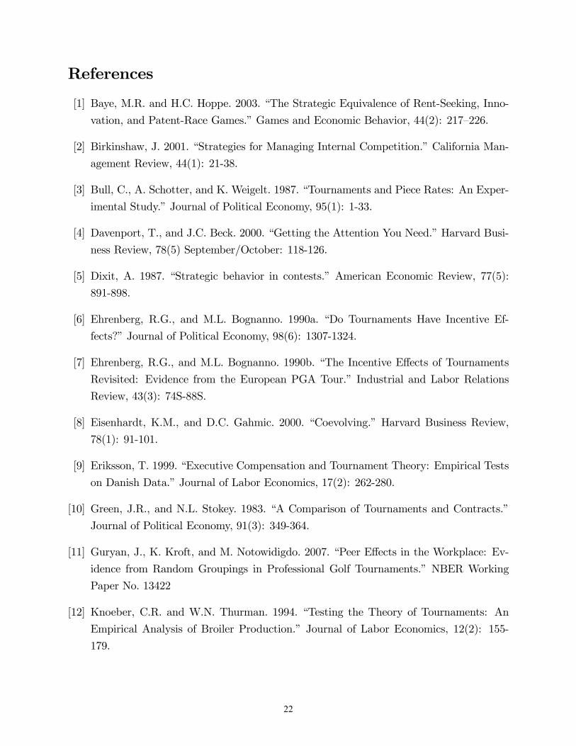
References
[1] Baye, M.R. and H.C. Hoppe. 2003. �The Strategic Equivalence of Rent-Seeking, Inno-
vation, and Patent-Race Games.�Games and Economic Behavior, 44(2): 217�226.
[2] Birkinshaw, J. 2001. �Strategies for Managing Internal Competition.�California Man-
agement Review, 44(1): 21-38.
[3] Bull, C., A. Schotter, and K. Weigelt. 1987. �Tournaments and Piece Rates: An Exper-
imental Study.�Journal of Political Economy, 95(1): 1-33.
[4] Davenport, T., and J.C. Beck. 2000. �Getting the Attention You Need.�Harvard Busi-
ness Review, 78(5) September/October: 118-126.
[5] Dixit, A. 1987. �Strategic behavior in contests.� American Economic Review, 77(5):
891-898.
[6] Ehrenberg, R.G., and M.L. Bognanno. 1990a. �Do Tournaments Have Incentive Ef-
fects?�Journal of Political Economy, 98(6): 1307-1324.
[7] Ehrenberg, R.G., and M.L. Bognanno. 1990b. �The Incentive E¤ects of Tournaments
Revisited: Evidence from the European PGA Tour.� Industrial and Labor Relations
Review, 43(3): 74S-88S.
[8] Eisenhardt, K.M., and D.C. Gahmic. 2000. �Coevolving.�Harvard Business Review,
78(1): 91-101.
[9] Eriksson, T. 1999. �Executive Compensation and Tournament Theory: Empirical Tests
on Danish Data.�Journal of Labor Economics, 17(2): 262-280.
[10] Green, J.R., and N.L. Stokey. 1983. �A Comparison of Tournaments and Contracts.�
Journal of Political Economy, 91(3): 349-364.
[11] Guryan, J., K. Kroft, and M. Notowidigdo. 2007. �Peer E¤ects in the Workplace: Ev-
idence from Random Groupings in Professional Golf Tournaments.� NBER Working
Paper No. 13422
[12] Knoeber, C.R. and W.N. Thurman. 1994. �Testing the Theory of Tournaments: An
Empirical Analysis of Broiler Production.� Journal of Labor Economics, 12(2): 155-
179.
22
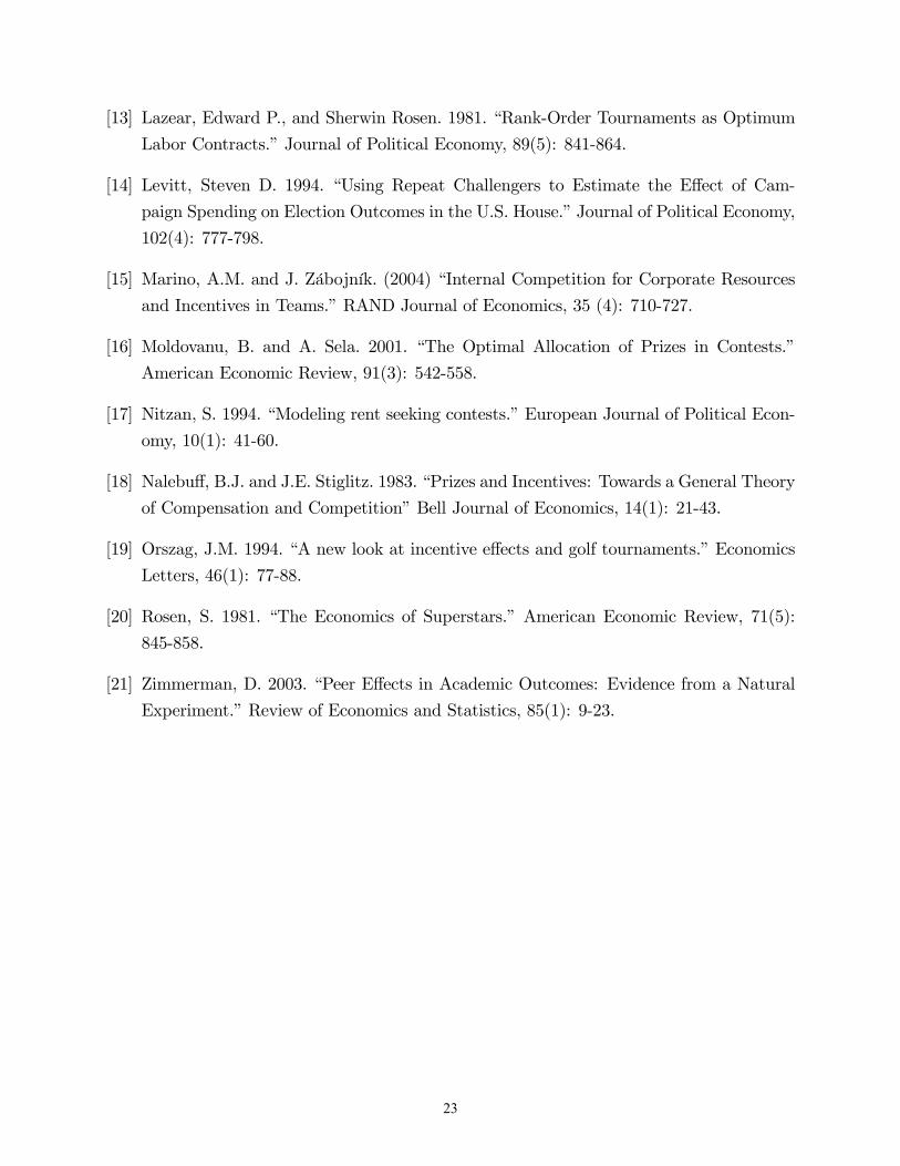
[13] Lazear, Edward P., and Sherwin Rosen. 1981. �Rank-Order Tournaments as Optimum
Labor Contracts.�Journal of Political Economy, 89(5): 841-864.
[14] Levitt, Steven D. 1994. �Using Repeat Challengers to Estimate the E¤ect of Cam-
paign Spending on Election Outcomes in the U.S. House.�Journal of Political Economy,
102(4): 777-798.
[15] Marino, A.M. and J. Zábojník. (2004) �Internal Competition for Corporate Resources
and Incentives in Teams.�RAND Journal of Economics, 35 (4): 710-727.
[16] Moldovanu, B. and A. Sela. 2001. �The Optimal Allocation of Prizes in Contests.�
American Economic Review, 91(3): 542-558.
[17] Nitzan, S. 1994. �Modeling rent seeking contests.�European Journal of Political Econ-
omy, 10(1): 41-60.
[18] Nalebu¤, B.J. and J.E. Stiglitz. 1983. �Prizes and Incentives: Towards a General Theory
of Compensation and Competition�Bell Journal of Economics, 14(1): 21-43.
[19] Orszag, J.M. 1994. �A new look at incentive e¤ects and golf tournaments.�Economics
Letters, 46(1): 77-88.
[20] Rosen, S. 1981. �The Economics of Superstars.� American Economic Review, 71(5):
845-858.
[21] Zimmerman, D. 2003. �Peer E¤ects in Academic Outcomes: Evidence from a Natural
Experiment.�Review of Economics and Statistics, 85(1): 9-23.
23
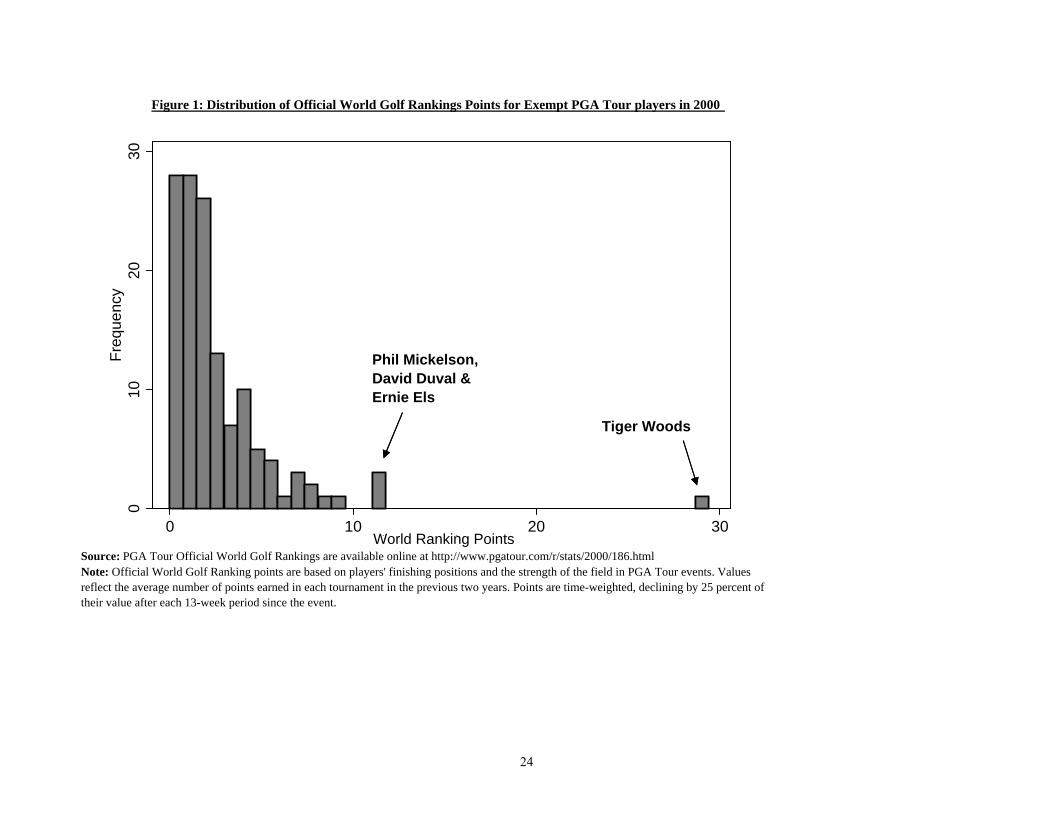
Figure 1: Distribution of Official World Golf Rankings Points for Exempt PGA Tour players in 2000
010
2030
Freq
uenc
y
0 10 20 30( ) k i
Tiger Woods
Phil Mickelson, David Duval & Ernie Els
Source: PGA Tour Official World Golf Rankings are available online at http://www.pgatour.com/r/stats/2000/186.htmlNote: Official World Golf Ranking points are based on players' finishing positions and the strength of the field in PGA Tour events. Values reflect the average number of points earned in each tournament in the previous two years. Points are time-weighted, declining by 25 percent of their value after each 13-week period since the event.
World Ranking Points
24
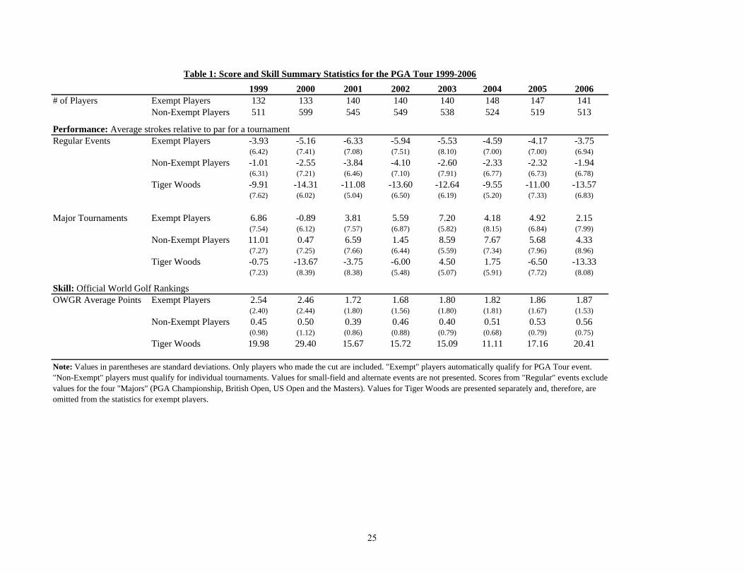
Table 1: Score and Skill Summary Statistics for the PGA Tour 1999-20061999 2000 2001 2002 2003 2004 2005 2006
# of Players Exempt Players 132 133 140 140 140 148 147 141Non-Exempt Players 511 599 545 549 538 524 519 513
Performance: Average strokes relative to par for a tournamentRegular Events Exempt Players -3.93 -5.16 -6.33 -5.94 -5.53 -4.59 -4.17 -3.75
(6.42) (7.41) (7.08) (7.51) (8.10) (7.00) (7.00) (6.94)Non-Exempt Players -1.01 -2.55 -3.84 -4.10 -2.60 -2.33 -2.32 -1.94
(6.31) (7.21) (6.46) (7.10) (7.91) (6.77) (6.73) (6.78)Tiger Woods -9.91 -14.31 -11.08 -13.60 -12.64 -9.55 -11.00 -13.57
(7.62) (6.02) (5.04) (6.50) (6.19) (5.20) (7.33) (6.83)
Major Tournaments Exempt Players 6.86 -0.89 3.81 5.59 7.20 4.18 4.92 2.15(7.54) (6.12) (7.57) (6.87) (5.82) (8.15) (6.84) (7.99)
Non-Exempt Players 11.01 0.47 6.59 1.45 8.59 7.67 5.68 4.33(7.27) (7.25) (7.66) (6.44) (5.59) (7.34) (7.96) (8.96)
Tiger Woods -0.75 -13.67 -3.75 -6.00 4.50 1.75 -6.50 -13.33(7.23) (8.39) (8.38) (5.48) (5.07) (5.91) (7.72) (8.08)
Skill: Official World Golf RankingsOWGR Average Points Exempt Players 2.54 2.46 1.72 1.68 1.80 1.82 1.86 1.87
(2.40) (2.44) (1.80) (1.56) (1.80) (1.81) (1.67) (1.53)Non-Exempt Players 0.45 0.50 0.39 0.46 0.40 0.51 0.53 0.56
(0.98) (1.12) (0.86) (0.88) (0.79) (0.68) (0.79) (0.75)Tiger Woods 19.98 29.40 15.67 15.72 15.09 11.11 17.16 20.41
Note: Values in parentheses are standard deviations. Only players who made the cut are included. "Exempt" players automatically qualify for PGA Tour event. "Non-Exempt" players must qualify for individual tournaments. Values for small-field and alternate events are not presented. Scores from "Regular" events exclude values for the four "Majors" (PGA Championship, British Open, US Open and the Masters). Values for Tiger Woods are presented separately and, therefore, are omitted from the statistics for exempt players.
25
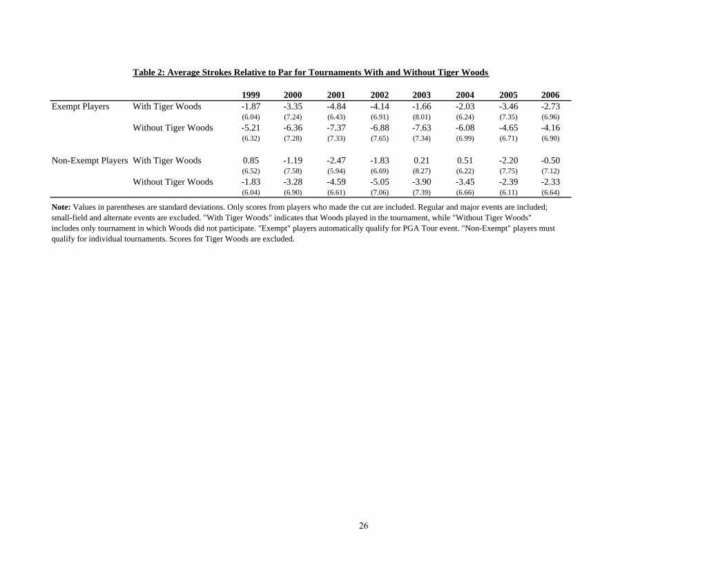
Table 2: Average Strokes Relative to Par for Tournaments With and Without Tiger Woods
1999 2000 2001 2002 2003 2004 2005 2006Exempt Players With Tiger Woods -1.87 -3.35 -4.84 -4.14 -1.66 -2.03 -3.46 -2.73
(6.04) (7.24) (6.43) (6.91) (8.01) (6.24) (7.35) (6.96)Without Tiger Woods -5.21 -6.36 -7.37 -6.88 -7.63 -6.08 -4.65 -4.16
(6.32) (7.28) (7.33) (7.65) (7.34) (6.99) (6.71) (6.90)
Non-Exempt Players With Tiger Woods 0.85 -1.19 -2.47 -1.83 0.21 0.51 -2.20 -0.50(6.52) (7.58) (5.94) (6.69) (8.27) (6.22) (7.75) (7.12)
Without Tiger Woods -1.83 -3.28 -4.59 -5.05 -3.90 -3.45 -2.39 -2.33(6.04) (6.90) (6.61) (7.06) (7.39) (6.66) (6.11) (6.64)
Note: Values in parentheses are standard deviations. Only scores from players who made the cut are included. Regular and major events are included; small-field and alternate events are excluded. "With Tiger Woods" indicates that Woods played in the tournament, while "Without Tiger Woods" includes only tournament in which Woods did not participate. "Exempt" players automatically qualify for PGA Tour event. "Non-Exempt" players must qualify for individual tournaments. Scores for Tiger Woods are excluded.
26
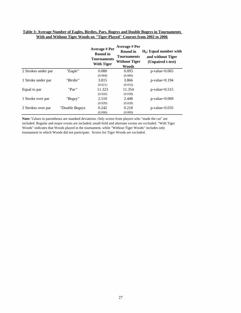
Table 3: Average Number of Eagles, Birdies, Pars, Bogeys and Double Bogeys in Tournaments With and Without Tiger Woods on "Tiger-Played" Courses from 2002 to 2006
Average # Per Round in
Tournaments With Tiger
Average # Per Round in
Tournaments Without Tiger
Woods
H0: Equal number with and without Tiger (Unpaired t-test)
2 Strokes under par "Eagle" 0.080 0.093 p-value=0.065(0.004) (0.006)
1 Stroke under par "Birdie" 3.815 3.866 p-value=0.194(0.021) (0.033)
Equal to par "Par" 11.323 11.354 p-value=0.515(0.026) (0.038)
1 Stroke over par "Bogey" 2.510 2.448 p-value=0.069(0.020) (0.028)
2 Strokes over par "Double Bogeys 0.242 0.218 p-value=0.035(0.006) (0.009)
Note: Values in parentheses are standard deviations. Only scores from players who "made the cut" are included. Regular and major events are included; small-field and alternate events are excluded. "With Tiger Woods" indicates that Woods played in the tournament, while "Without Tiger Woods" includes only tournament in which Woods did not participate. Scores for Tiger Woods are excluded.
27
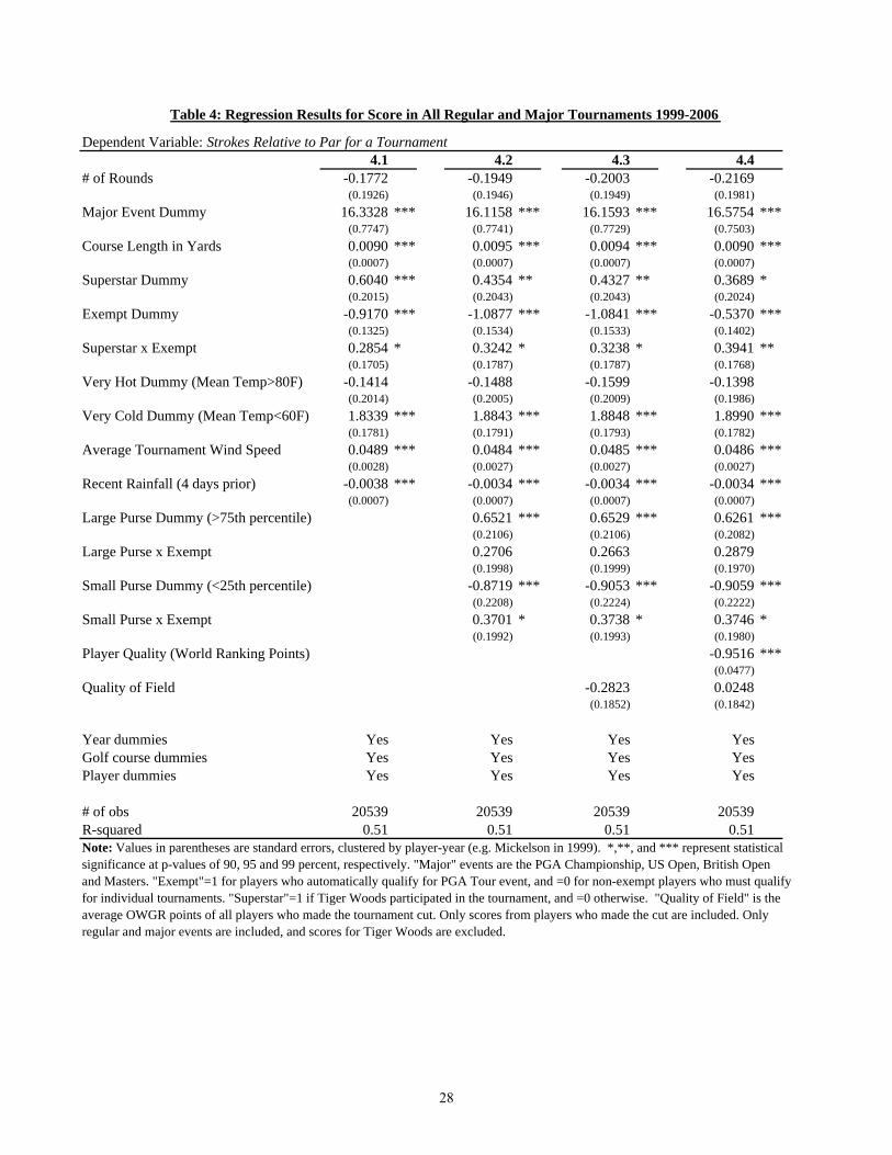
Table 4: Regression Results for Score in All Regular and Major Tournaments 1999-2006
Dependent Variable: Strokes Relative to Par for a Tournament4.1 4.2 4.3 4.4
# of Rounds -0.1772 -0.1949 -0.2003 -0.2169(0.1926) (0.1946) (0.1949) (0.1981)
Major Event Dummy 16.3328 *** 16.1158 *** 16.1593 *** 16.5754 ***(0.7747) (0.7741) (0.7729) (0.7503)
Course Length in Yards 0.0090 *** 0.0095 *** 0.0094 *** 0.0090 ***(0.0007) (0.0007) (0.0007) (0.0007)
Superstar Dummy 0.6040 *** 0.4354 ** 0.4327 ** 0.3689 *(0.2015) (0.2043) (0.2043) (0.2024)
Exempt Dummy -0.9170 *** -1.0877 *** -1.0841 *** -0.5370 ***(0.1325) (0.1534) (0.1533) (0.1402)
Superstar x Exempt 0.2854 * 0.3242 * 0.3238 * 0.3941 **(0.1705) (0.1787) (0.1787) (0.1768)
Very Hot Dummy (Mean Temp>80F) -0.1414 -0.1488 -0.1599 -0.1398(0.2014) (0.2005) (0.2009) (0.1986)
Very Cold Dummy (Mean Temp<60F) 1.8339 *** 1.8843 *** 1.8848 *** 1.8990 ***(0.1781) (0.1791) (0.1793) (0.1782)
Average Tournament Wind Speed 0.0489 *** 0.0484 *** 0.0485 *** 0.0486 ***(0.0028) (0.0027) (0.0027) (0.0027)
Recent Rainfall (4 days prior) -0.0038 *** -0.0034 *** -0.0034 *** -0.0034 ***(0.0007) (0.0007) (0.0007) (0.0007)
Large Purse Dummy (>75th percentile) 0.6521 *** 0.6529 *** 0.6261 ***(0.2106) (0.2106) (0.2082)
Large Purse x Exempt 0.2706 0.2663 0.2879(0.1998) (0.1999) (0.1970)
Small Purse Dummy (<25th percentile) -0.8719 *** -0.9053 *** -0.9059 ***(0.2208) (0.2224) (0.2222)
Small Purse x Exempt 0.3701 * 0.3738 * 0.3746 *(0.1992) (0.1993) (0.1980)
Player Quality (World Ranking Points) -0.9516 ***(0.0477)
Quality of Field -0.2823 0.0248(0.1852) (0.1842)
Year dummies Yes Yes Yes YesGolf course dummies Yes Yes Yes YesPlayer dummies Yes Yes Yes Yes
# of obs 20539 20539 20539 20539R-squared 0.51 0.51 0.51 0.51Note: Values in parentheses are standard errors, clustered by player-year (e.g. Mickelson in 1999). *,**, and *** represent statistical significance at p-values of 90, 95 and 99 percent, respectively. "Major" events are the PGA Championship, US Open, British Open and Masters. "Exempt"=1 for players who automatically qualify for PGA Tour event, and =0 for non-exempt players who must qualifyfor individual tournaments. "Superstar"=1 if Tiger Woods participated in the tournament, and =0 otherwise. "Quality of Field" is the average OWGR points of all players who made the tournament cut. Only scores from players who made the cut are included. Only regular and major events are included, and scores for Tiger Woods are excluded.
28
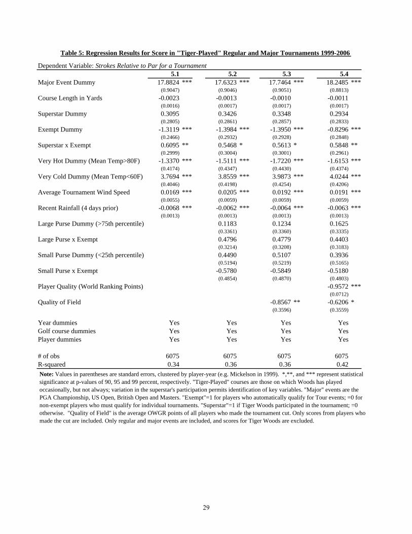
Table 5: Regression Results for Score in "Tiger-Played" Regular and Major Tournaments 1999-2006
Dependent Variable: Strokes Relative to Par for a Tournament5.1 5.2 5.3 5.4
Major Event Dummy 17.8824 *** 17.6323 *** 17.7464 *** 18.2485 ***(0.9047) (0.9046) (0.9051) (0.8813)
Course Length in Yards -0.0023 -0.0013 -0.0010 -0.0011(0.0016) (0.0017) (0.0017) (0.0017)
Superstar Dummy 0.3095 0.3426 0.3348 0.2934(0.2805) (0.2861) (0.2857) (0.2833)
Exempt Dummy -1.3119 *** -1.3984 *** -1.3950 *** -0.8296 ***(0.2466) (0.2932) (0.2928) (0.2848)
Superstar x Exempt 0.6095 ** 0.5468 * 0.5613 * 0.5848 **(0.2999) (0.3004) (0.3001) (0.2961)
Very Hot Dummy (Mean Temp>80F) -1.3370 *** -1.5111 *** -1.7220 *** -1.6153 ***(0.4174) (0.4347) (0.4430) (0.4374)
Very Cold Dummy (Mean Temp<60F) 3.7694 *** 3.8559 *** 3.9873 *** 4.0244 ***(0.4046) (0.4198) (0.4254) (0.4206)
Average Tournament Wind Speed 0.0169 *** 0.0205 *** 0.0192 *** 0.0191 ***(0.0055) (0.0059) (0.0059) (0.0059)
Recent Rainfall (4 days prior) -0.0068 *** -0.0062 *** -0.0064 *** -0.0063 ***(0.0013) (0.0013) (0.0013) (0.0013)
Large Purse Dummy (>75th percentile) 0.1183 0.1234 0.1625(0.3361) (0.3360) (0.3335)
Large Purse x Exempt 0.4796 0.4779 0.4403(0.3214) (0.3208) (0.3183)
Small Purse Dummy (<25th percentile) 0.4490 0.5107 0.3936(0.5194) (0.5219) (0.5165)
Small Purse x Exempt -0.5780 -0.5849 -0.5180(0.4854) (0.4870) (0.4803)
Player Quality (World Ranking Points) -0.9572 ***(0.0712)
Quality of Field -0.8567 ** -0.6206 *(0.3596) (0.3559)
Year dummies Yes Yes Yes YesGolf course dummies Yes Yes Yes YesPlayer dummies Yes Yes Yes Yes
# of obs 6075 6075 6075 6075R-squared 0.34 0.36 0.36 0.42Note: Values in parentheses are standard errors, clustered by player-year (e.g. Mickelson in 1999). *,**, and *** represent statistical significance at p-values of 90, 95 and 99 percent, respectively. "Tiger-Played" courses are those on which Woods has played occasionally, but not always; variation in the superstar's participation permits identification of key variables. "Major" events are the PGA Championship, US Open, British Open and Masters. "Exempt"=1 for players who automatically qualify for Tour events; =0 for non-exempt players who must qualify for individual tournaments. "Superstar"=1 if Tiger Woods participated in the tournament; =0 otherwise. "Quality of Field" is the average OWGR points of all players who made the tournament cut. Only scores from players who made the cut are included. Only regular and major events are included, and scores for Tiger Woods are excluded.
29
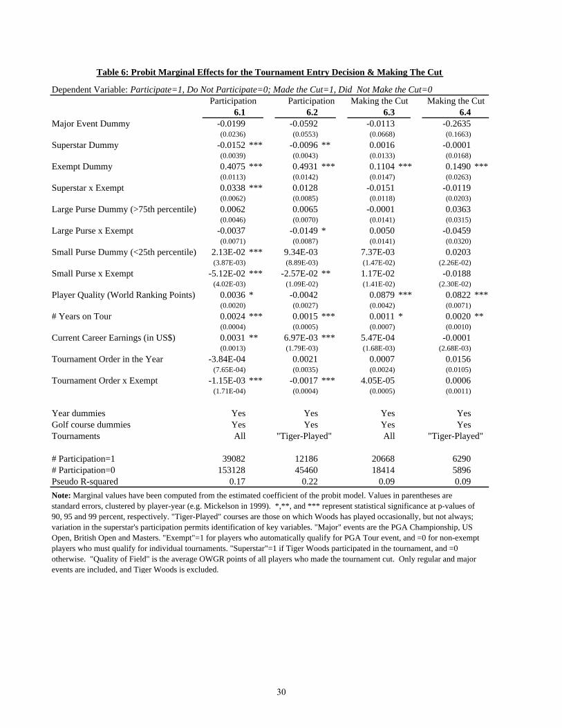
Table 6: Probit Marginal Effects for the Tournament Entry Decision & Making The Cut
Dependent Variable: Participate=1, Do Not Participate=0; Made the Cut=1, Did Not Make the Cut=0Participation Participation Making the Cut Making the Cut
6.1 6.2 6.3 6.4Major Event Dummy -0.0199 -0.0592 -0.0113 -0.2635
(0.0236) (0.0553) (0.0668) (0.1663)Superstar Dummy -0.0152 *** -0.0096 ** 0.0016 -0.0001
(0.0039) (0.0043) (0.0133) (0.0168)Exempt Dummy 0.4075 *** 0.4931 *** 0.1104 *** 0.1490 ***
(0.0113) (0.0142) (0.0147) (0.0263)Superstar x Exempt 0.0338 *** 0.0128 -0.0151 -0.0119
(0.0062) (0.0085) (0.0118) (0.0203)Large Purse Dummy (>75th percentile) 0.0062 0.0065 -0.0001 0.0363
(0.0046) (0.0070) (0.0141) (0.0315)Large Purse x Exempt -0.0037 -0.0149 * 0.0050 -0.0459
(0.0071) (0.0087) (0.0141) (0.0320)Small Purse Dummy (<25th percentile) 2.13E-02 *** 9.34E-03 7.37E-03 0.0203
(3.87E-03) (8.89E-03) (1.47E-02) (2.26E-02)Small Purse x Exempt -5.12E-02 *** -2.57E-02 ** 1.17E-02 -0.0188
(4.02E-03) (1.09E-02) (1.41E-02) (2.30E-02)Player Quality (World Ranking Points) 0.0036 * -0.0042 0.0879 *** 0.0822 ***
(0.0020) (0.0027) (0.0042) (0.0071)# Years on Tour 0.0024 *** 0.0015 *** 0.0011 * 0.0020 **
(0.0004) (0.0005) (0.0007) (0.0010)Current Career Earnings (in US$) 0.0031 ** 6.97E-03 *** 5.47E-04 -0.0001
(0.0013) (1.79E-03) (1.68E-03) (2.68E-03)Tournament Order in the Year -3.84E-04 0.0021 0.0007 0.0156
(7.65E-04) (0.0035) (0.0024) (0.0105)Tournament Order x Exempt -1.15E-03 *** -0.0017 *** 4.05E-05 0.0006
(1.71E-04) (0.0004) (0.0005) (0.0011)
Year dummies Yes Yes Yes YesGolf course dummies Yes Yes Yes YesTournaments All "Tiger-Played" All "Tiger-Played"
# Participation=1 39082 12186 20668 6290# Participation=0 153128 45460 18414 5896Pseudo R-squared 0.17 0.22 0.09 0.09Note: Marginal values have been computed from the estimated coefficient of the probit model. Values in parentheses are standard errors, clustered by player-year (e.g. Mickelson in 1999). *,**, and *** represent statistical significance at p-values of 90, 95 and 99 percent, respectively. "Tiger-Played" courses are those on which Woods has played occasionally, but not always; variation in the superstar's participation permits identification of key variables. "Major" events are the PGA Championship, US Open, British Open and Masters. "Exempt"=1 for players who automatically qualify for PGA Tour event, and =0 for non-exempt players who must qualify for individual tournaments. "Superstar"=1 if Tiger Woods participated in the tournament, and =0 otherwise. "Quality of Field" is the average OWGR points of all players who made the tournament cut. Only regular and major events are included, and Tiger Woods is excluded.
30
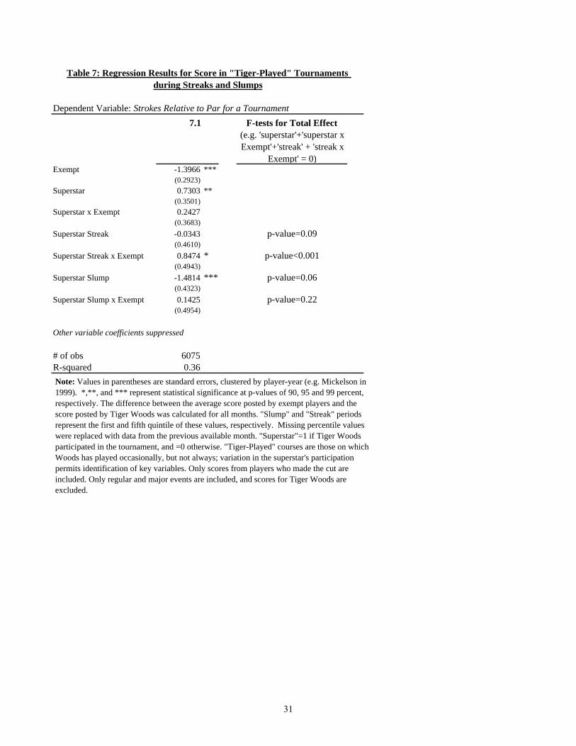
Table 7: Regression Results for Score in "Tiger-Played" Tournaments during Streaks and Slumps
Dependent Variable: Strokes Relative to Par for a Tournament7.1 F-tests for Total Effect
(e.g. 'superstar'+'superstar x Exempt'+'streak' + 'streak x
Exempt' = 0)Exempt -1.3966 ***
(0.2923)Superstar 0.7303 **
(0.3501)Superstar x Exempt 0.2427
(0.3683)Superstar Streak -0.0343 p-value=0.09
(0.4610)Superstar Streak x Exempt 0.8474 * p-value<0.001
(0.4943)Superstar Slump -1.4814 *** p-value=0.06
(0.4323)Superstar Slump x Exempt 0.1425 p-value=0.22
(0.4954)
Other variable coefficients suppressed
# of obs 6075R-squared 0.36Note: Values in parentheses are standard errors, clustered by player-year (e.g. Mickelson in 1999). *,**, and *** represent statistical significance at p-values of 90, 95 and 99 percent, respectively. The difference between the average score posted by exempt players and the score posted by Tiger Woods was calculated for all months. "Slump" and "Streak" periods represent the first and fifth quintile of these values, respectively. Missing percentile values were replaced with data from the previous available month. "Superstar"=1 if Tiger Woods participated in the tournament, and =0 otherwise. "Tiger-Played" courses are those on which Woods has played occasionally, but not always; variation in the superstar's participation permits identification of key variables. Only scores from players who made the cut are included. Only regular and major events are included, and scores for Tiger Woods are excluded.
31
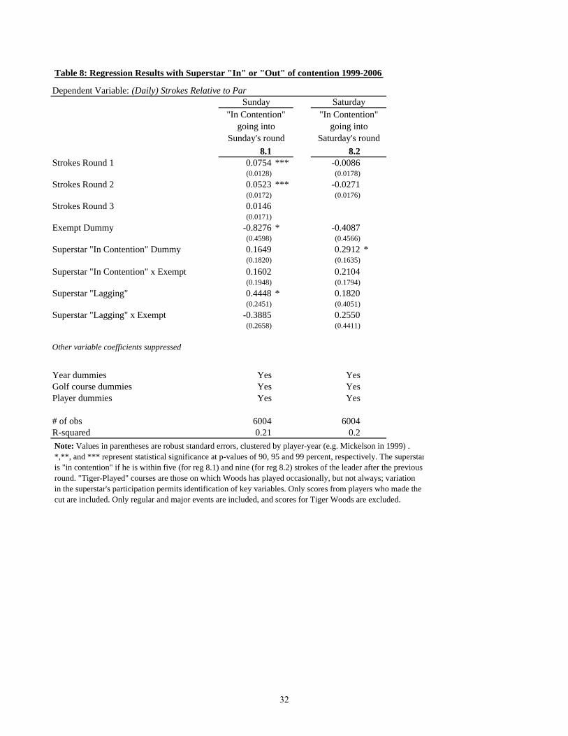
Table 8: Regression Results with Superstar "In" or "Out" of contention 1999-2006
Dependent Variable: (Daily) Strokes Relative to Par Sunday Saturday
"In Contention" going into
Sunday's round
"In Contention" going into
Saturday's round8.1 8.2
Strokes Round 1 0.0754 *** -0.0086(0.0128) (0.0178)
Strokes Round 2 0.0523 *** -0.0271(0.0172) (0.0176)
Strokes Round 3 0.0146(0.0171)
Exempt Dummy -0.8276 * -0.4087(0.4598) (0.4566)
Superstar "In Contention" Dummy 0.1649 0.2912 *(0.1820) (0.1635)
Superstar "In Contention" x Exempt 0.1602 0.2104(0.1948) (0.1794)
Superstar "Lagging" 0.4448 * 0.1820(0.2451) (0.4051)
Superstar "Lagging" x Exempt -0.3885 0.2550(0.2658) (0.4411)
Other variable coefficients suppressed
Year dummies Yes YesGolf course dummies Yes YesPlayer dummies Yes Yes
# of obs 6004 6004R-squared 0.21 0.2Note: Values in parentheses are robust standard errors, clustered by player-year (e.g. Mickelson in 1999) . *,**, and *** represent statistical significance at p-values of 90, 95 and 99 percent, respectively. The superstaris "in contention" if he is within five (for reg 8.1) and nine (for reg 8.2) strokes of the leader after the previous round. "Tiger-Played" courses are those on which Woods has played occasionally, but not always; variation in the superstar's participation permits identification of key variables. Only scores from players who made the cut are included. Only regular and major events are included, and scores for Tiger Woods are excluded.
32
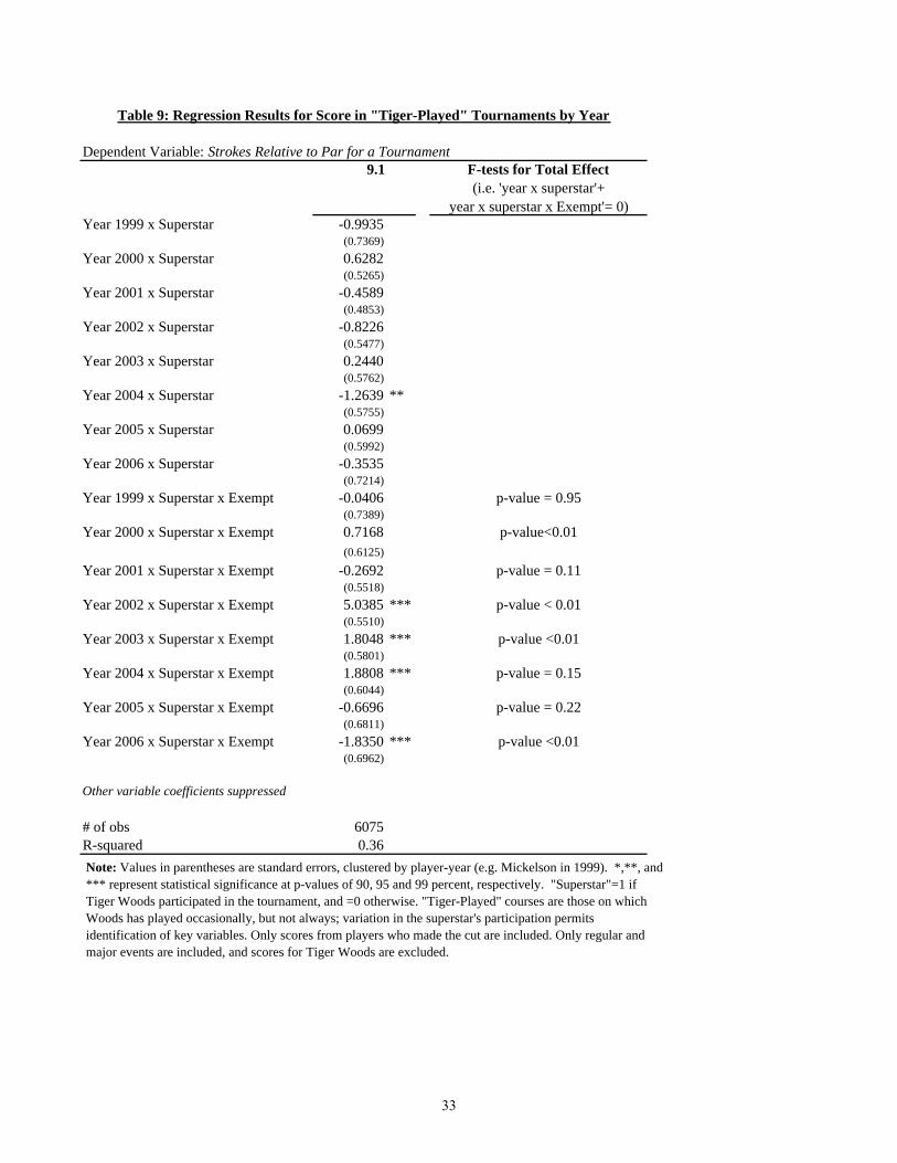
Table 9: Regression Results for Score in "Tiger-Played" Tournaments by Year
Dependent Variable: Strokes Relative to Par for a Tournament9.1 F-tests for Total Effect
(i.e. 'year x superstar'+ year x superstar x Exempt'= 0)
Year 1999 x Superstar -0.9935(0.7369)
Year 2000 x Superstar 0.6282(0.5265)
Year 2001 x Superstar -0.4589(0.4853)
Year 2002 x Superstar -0.8226(0.5477)
Year 2003 x Superstar 0.2440(0.5762)
Year 2004 x Superstar -1.2639 **(0.5755)
Year 2005 x Superstar 0.0699(0.5992)
Year 2006 x Superstar -0.3535(0.7214)
Year 1999 x Superstar x Exempt -0.0406 p-value = 0.95(0.7389)
Year 2000 x Superstar x Exempt 0.7168 p-value<0.01(0.6125)
Year 2001 x Superstar x Exempt -0.2692 p-value = 0.11(0.5518)
Year 2002 x Superstar x Exempt 5.0385 *** p-value < 0.01(0.5510)
Year 2003 x Superstar x Exempt 1.8048 *** p-value <0.01(0.5801)
Year 2004 x Superstar x Exempt 1.8808 *** p-value = 0.15(0.6044)
Year 2005 x Superstar x Exempt -0.6696 p-value = 0.22(0.6811)
Year 2006 x Superstar x Exempt -1.8350 *** p-value <0.01(0.6962)
Other variable coefficients suppressed
# of obs 6075R-squared 0.36Note: Values in parentheses are standard errors, clustered by player-year (e.g. Mickelson in 1999). *,**, and *** represent statistical significance at p-values of 90, 95 and 99 percent, respectively. "Superstar"=1 if Tiger Woods participated in the tournament, and =0 otherwise. "Tiger-Played" courses are those on which Woods has played occasionally, but not always; variation in the superstar's participation permits identification of key variables. Only scores from players who made the cut are included. Only regular and major events are included, and scores for Tiger Woods are excluded.
33
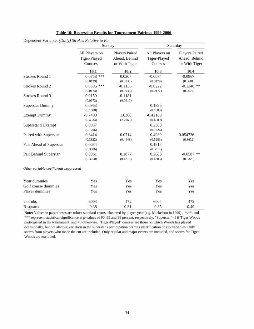
Table 10: Regression Results for Tournament Pairings 1999-2006
Dependent Variable: (Daily) Strokes Relative to Par Sunday Saturday
All Players on Tiger-Played
Courses
Players Paired Ahead, Behind or With Tiger
All Players on Tiger-Played
Courses
Players Paired Ahead, Behind or With Tiger
10.1 10.2 10.3 10.4Strokes Round 1 0.0758 *** 0.0207 -0.0074 -0.0967
(0.0129) (0.0838) (0.0179) (0.0681)Strokes Round 2 0.0506 *** -0.1136 -0.0222 -0.1346 **
(0.0174) (0.0936) (0.0177) (0.0672)Strokes Round 3 0.0150 -0.1181
(0.0172) (0.0919)Superstar Dummy 0.0963 0.1896
(0.1688) (0.1603)Exempt Dummy -0.7403 1.6360 -0.42189
(0.4534) (2.2068) (0.4509)Superstar x Exempt 0.0057 0.2388
(0.1796) (0.1726)Paired with Superstar -0.3414 -0.0714 0.4930 0.054726
(0.3822) (0.4448) (0.5283) (0.3632)Pair Ahead of Superstar 0.0684 0.1818
(0.3386) (0.3011)Pair Behind Superstar 0.3961 0.1877 0.2689 -0.6587 **
(0.3250) (0.4215) (0.4305) (0.3329)
Other variable coefficients suppressed
Year dummies Yes Yes Yes YesGolf course dummies Yes Yes Yes YesPlayer dummies Yes Yes Yes Yes
# of obs 6004 472 6004 472R-squared 0.38 0.31 0.35 0.49Note: Values in parentheses are robust standard errors, clustered by player-year (e.g. Mickelson in 1999) . *,**, and *** represent statistical significance at p-values of 90, 95 and 99 percent, respectively. "Superstar"=1 if Tiger Woods participated in the tournament, and =0 otherwise. "Tiger-Played" courses are those on which Woods has played occasionally, but not always; variation in the superstar's participation permits identification of key variables. Only scores from players who made the cut are included. Only regular and major events are included, and scores for Tiger Woods are excluded.
34
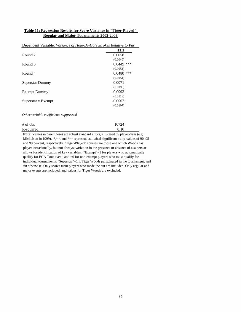
Table 11: Regression Results for Score Variance in "Tiger-Played" Regular and Major Tournaments 2002-2006
Dependent Variable: Variance of Hole-By-Hole Strokes Relative to Par11.1
Round 2 0.0058(0.0049)
Round 3 0.0449 ***(0.0051)
Round 4 0.0480 ***(0.0051)
Superstar Dummy 0.0071(0.0096)
Exempt Dummy -0.0092(0.0119)
Superstar x Exempt -0.0002(0.0107)
Other variable coefficients suppressed
# of obs 10724R-squared 0.10Note: Values in parentheses are robust standard errors, clustered by player-year (e.g. Mickelson in 1999). *,**, and *** represent statistical significance at p-values of 90, 95 and 99 percent, respectively. "Tiger-Played" courses are those one which Woods has played occasionally, but not always; variation in the presence or absence of a superstar allows for identification of key variables. "Exempt"=1 for players who automatically qualify for PGA Tour event, and =0 for non-exempt players who must qualify for individual tournaments. "Superstar"=1 if Tiger Woods participated in the tournament, and =0 otherwise. Only scores from players who made the cut are included. Only regular and major events are included, and values for Tiger Woods are excluded.
35