NBER WORKING PAPER SERIES

DECOMPOSITION METHODS IN ECONOMICS

Nicole FortinThomas Lemieux

Sergio Firpo

Working Paper 16045http://www.nber.org/papers/w16045

NATIONAL BUREAU OF ECONOMIC RESEARCH1050 Massachusetts Avenue

Cambridge, MA 02138June 2010

We are grateful to Orley Ashenfelter, David Card, Pat Kline, and Craig Riddell for useful comments,and to the Social Sciences and Humanities Research Council of Canada for Research Support. Theviews expressed herein are those of the authors and do not necessarily reflect the views of the NationalBureau of Economic Research.

© 2010 by Nicole Fortin, Thomas Lemieux, and Sergio Firpo. All rights reserved. Short sections oftext, not to exceed two paragraphs, may be quoted without explicit permission provided that full credit,including © notice, is given to the source.

Decomposition Methods in EconomicsNicole Fortin, Thomas Lemieux, and Sergio FirpoNBER Working Paper No. 16045June 2010JEL No. C14,C21,J31,J71

ABSTRACT

This chapter provides a comprehensive overview of decomposition methods that have been developedsince the seminal work of Oaxaca and Blinder in the early 1970s. These methods are used to decomposethe difference in a distributional statistic between two groups, or its change over time, into variousexplanatory factors. While the original work of Oaxaca and Blinder considered the case of the mean,our main focus is on other distributional statistics besides the mean such as quantiles, the Gini coefficient orthe variance. We discuss the assumptions required for identifying the different elements of the decomposition,as well as various estimation methods proposed in the literature. We also illustrate how these methodswork in practice by discussing existing applications and working through a set of empirical examplesthroughout the paper.

Nicole FortinDepartment of EconomicsUniversity of British Columbia#997-1873 East MallVancouver, BC V6T 1Z1Canadanifortin@interchange.ubc.ca

Thomas LemieuxDepartment of EconomicsUniversity of British Columbia#997-1873 East MallVancouver, BC V6T 1Z1Canadaand NBERtlemieux@interchange.ubc.ca

Sergio FirpoSão Paulo School of Economicssergio.firpo@fgv.br

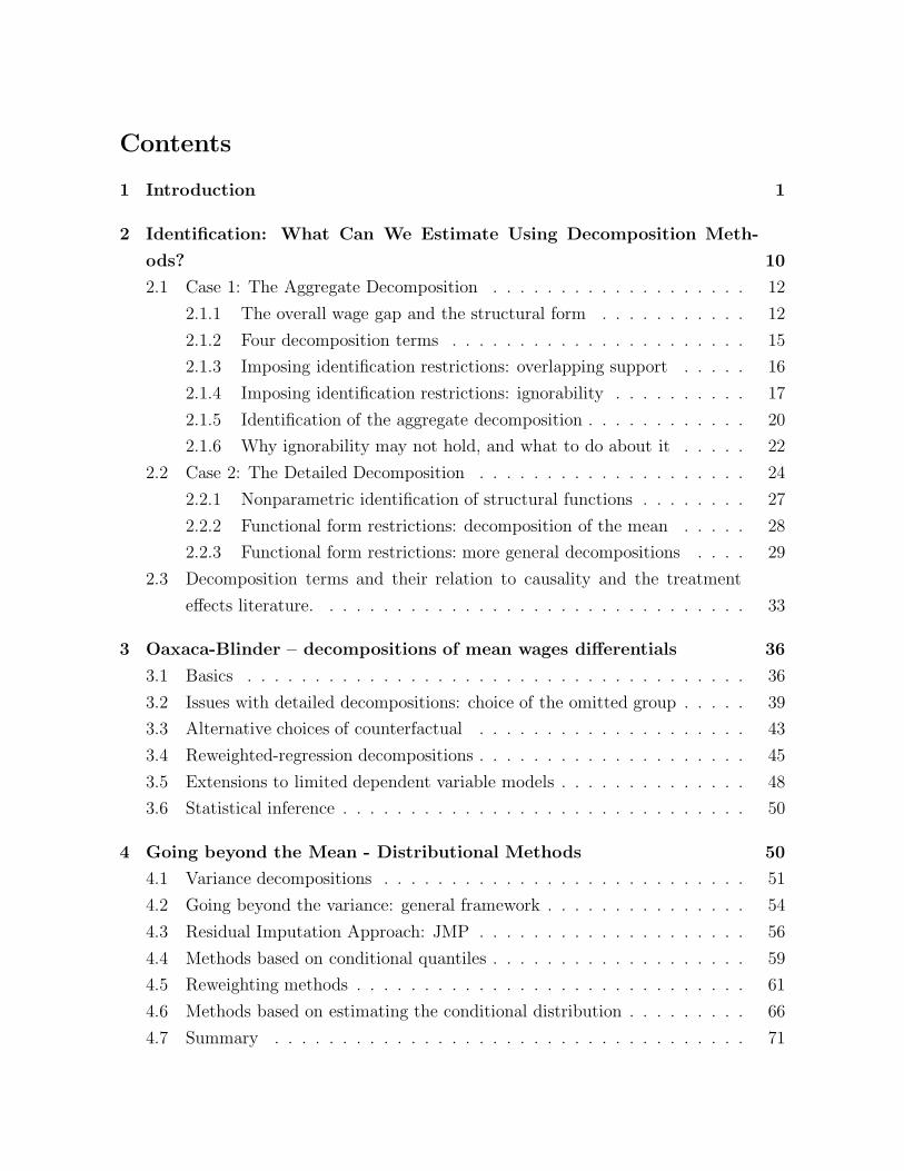
Contents

1 Introduction 1

2 Identification: What Can We Estimate Using Decomposition Meth-

ods? 10

2.1 Case 1: The Aggregate Decomposition . . . . . . . . . . . . . . . . . . . 12

2.1.1 The overall wage gap and the structural form . . . . . . . . . . . 12

2.1.2 Four decomposition terms . . . . . . . . . . . . . . . . . . . . . . 15

2.1.3 Imposing identification restrictions: overlapping support . . . . . 16

2.1.4 Imposing identification restrictions: ignorability . . . . . . . . . . 17

2.1.5 Identification of the aggregate decomposition . . . . . . . . . . . . 20

2.1.6 Why ignorability may not hold, and what to do about it . . . . . 22

2.2 Case 2: The Detailed Decomposition . . . . . . . . . . . . . . . . . . . . 24

2.2.1 Nonparametric identification of structural functions . . . . . . . . 27

2.2.2 Functional form restrictions: decomposition of the mean . . . . . 28

2.2.3 Functional form restrictions: more general decompositions . . . . 29

2.3 Decomposition terms and their relation to causality and the treatment

effects literature. . . . . . . . . . . . . . . . . . . . . . . . . . . . . . . . 33

3 Oaxaca-Blinder – decompositions of mean wages differentials 36

3.1 Basics . . . . . . . . . . . . . . . . . . . . . . . . . . . . . . . . . . . . . 36

3.2 Issues with detailed decompositions: choice of the omitted group . . . . . 39

3.3 Alternative choices of counterfactual . . . . . . . . . . . . . . . . . . . . 43

3.4 Reweighted-regression decompositions . . . . . . . . . . . . . . . . . . . . 45

3.5 Extensions to limited dependent variable models . . . . . . . . . . . . . . 48

3.6 Statistical inference . . . . . . . . . . . . . . . . . . . . . . . . . . . . . . 50

4 Going beyond the Mean - Distributional Methods 50

4.1 Variance decompositions . . . . . . . . . . . . . . . . . . . . . . . . . . . 51

4.2 Going beyond the variance: general framework . . . . . . . . . . . . . . . 54

4.3 Residual Imputation Approach: JMP . . . . . . . . . . . . . . . . . . . . 56

4.4 Methods based on conditional quantiles . . . . . . . . . . . . . . . . . . . 59

4.5 Reweighting methods . . . . . . . . . . . . . . . . . . . . . . . . . . . . . 61

4.6 Methods based on estimating the conditional distribution . . . . . . . . . 66

4.7 Summary . . . . . . . . . . . . . . . . . . . . . . . . . . . . . . . . . . . 71

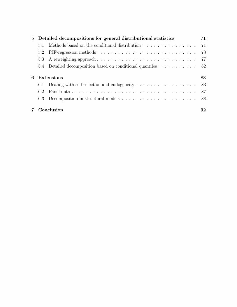
5 Detailed decompositions for general distributional statistics 71

5.1 Methods based on the conditional distribution . . . . . . . . . . . . . . . 71

5.2 RIF-regression methods . . . . . . . . . . . . . . . . . . . . . . . . . . . 73

5.3 A reweighting approach . . . . . . . . . . . . . . . . . . . . . . . . . . . . 77

5.4 Detailed decomposition based on conditional quantiles . . . . . . . . . . 82

6 Extensions 83

6.1 Dealing with self-selection and endogeneity . . . . . . . . . . . . . . . . . 83

6.2 Panel data . . . . . . . . . . . . . . . . . . . . . . . . . . . . . . . . . . . 87

6.3 Decomposition in structural models . . . . . . . . . . . . . . . . . . . . . 88

7 Conclusion 92

1 Introduction

What are the most important explanations accounting for pay di¤erences between men

and women? To what extent has wage inequality increased in the United States between

1980 and 2010 because of increasing returns to skill? Which factors are behind most of

the growth in U.S. GDP over the last 100 years? These important questions all share

a common feature. They are typically answered using decomposition methods. The

growth accounting approach pioneered by Solow (1957) and others is an early example

of a decomposition approach aimed at quantifying the contribution of labor, capital, and

unexplained factors (productivity) to U.S. growth.1 But it is in labor economics, starting

with the seminal papers of Oaxaca (1973) and Blinder (1973), that decomposition meth-

ods have been used the most extensively. These two papers are among the most heavily

cited in labor economics, and the Oaxaca-Blinder (OB) decomposition is now a stan-

dard tool in the toolkit of applied economists. A large number of methodological papers

aimed at re�ning the OB decomposition, and expanding it to the case of distributional

parameters besides the mean have also been written over the last three decades.

The twin goals of this chapter are to provide a comprehensive overview of decomposi-

tion methods that have been developed since the seminal work of Oaxaca and Blinder, and

to suggest a list of best practices for researchers interested in applying these methods.2

We also illustrate how these methods work in practice by discussing existing applications

and working through a set of empirical examples throughout the chapter.

At the outset, it is important to note a number of limitations to decomposition meth-

ods that are, by and large, beyond the scope of this chapter. As the above examples

show, the goal of decomposition methods are often quite ambitious, which means that

strong assumptions typically underlie these types of exercises. In particular, decompo-

sition methods inherently follow a partial equilibrium approach. Take, for instance, the

question �what would happen to average wages in the absence of unions?�As H. Gregg

Lewis pointed out a long time ago (Lewis, 1963, 1986), there are many reasons to believe

that eliminating unions would change not only the wages of union workers, but also those

of non-union workers. In this setting, the observed wage structure in the non-union sec-

tor would not represent a proper counterfactual for the wages observed in the absence of

1See also Kendrick (1961), Denison (1962), and Jorgenson and Griliches (1967).2We limit our discussion to so-called �regression-based" decomposition methods where the decom-

position focuses on explanatory factors, rather than decomposition methods that apply to additivelydecomposable indices where the decomposition pertains to population sub-groups. Bourguignon andFerreira (2005) and Bourguignon, Ferreira, and Leite (2008) are recent surveys discussing these meth-ods.

1

unions. We discuss these general equilibrium considerations in more detail towards the

end of the paper, but generally follow the standard partial equilibrium approach where

observed outcomes for one group (or region/time period) can be used to construct various

counterfactual scenarios for the other group.

A second important limitation is that while decompositions are useful for quantifying

the contribution of various factors to a di¤erence or change in outcomes in an accounting

sense, they may not necessarily deepen our understanding of the mechanisms underlying

the relationship between factors and outcomes. In that sense, decomposition methods,

just like program evaluation methods, do not seek to recover behavioral relationships or

�deep�structural parameters. By indicating which factors are quantitatively important

and which are not, however, decompositions provide useful indications of particular hy-

potheses or explanations to be explored in more detail. For example, if a decomposition

indicates that di¤erences in occupational a¢ liation account for a large fraction of the

gender wage gap, this suggests exploring in more detail how men and women choose

their �elds of study and occupations.

Another common use of decompositions is to provide some �bottom line�numbers

showing the quantitative importance of particular empirical estimates obtained in a study.

For example, while studies after studies show large and statistically signi�cant returns

to education, formal decompositions indicate that only a small fraction of U.S. growth,

or cross-country di¤erences, in GDP per capita can be accounted for by changes or

di¤erences in educational achievement.

Main themes and road map to the chapter

The original method proposed by Oaxaca and Blinder for decomposing changes or

di¤erences in the mean of an outcome variable has been considerably improved and

expanded upon over the years. Arguably, the most important development has been to

extend decomposition methods to distributional parameters other than the mean. For

instance, Freeman (1980, 1984) went beyond a simple decomposition of the di¤erence

in mean wages between the union and non-union sector to look at the di¤erence in the

variance of wages between the two sectors.

But it is the dramatic increase in wage inequality observed in the United States and

several other countries since the late 1970s that has been the main driving force behind

the development of a new set of decomposition methods. In particular, the new methods

introduced by Juhn, Murphy and Pierce (1993) and DiNardo, Fortin and Lemieux (1996)

were directly motivated by an attempt at better understanding the underlying factors

behind inequality growth. Going beyond the mean introduces a number of important

2

econometric challenges and is still an active area of research. As a result, we spend a

signi�cant portion of the chapter on these issues.

A second important development has been to use various tools from the program

evaluation literature to i) clarify the assumptions underneath popular decomposition

methods, ii) propose estimators for some of the elements of the decomposition, and iii)

obtain formal results on the statistical properties of the various decomposition terms.

As we explain below, the key connection with the treatment e¤ect literature is that the

�unexplained�component of a Oaxaca decomposition can be interpreted as a treatment

e¤ect. Note that, despite the interesting parallel with the program evaluation literature,

we explain in the paper that we cannot generally give a �causal� interpretation to the

decomposition results.

The chapter also covers a number of other practical issues that often arise when

working with decomposition methods. Those include the well known omitted group

problem (Oaxaca and Ransom, 1999), and how to deal with cases where we suspect the

true regression equation not to be linear.

Before getting into the details of the chapter, we provide here an overview of our

main contributions by relating them to the original OB decomposition for the di¤erence

in mean outcomes for two groups A and B. The standard assumption used in these

decompositions is that the outcome variable Y is linearly related to the covariates, X,

and that the error term � is conditionally independent of X:

Ygi = �g0 +KXk=1

Xik�gk + �gi; g = A;B; (1)

where E(�gijXi) = 0, and X is the vector of covariates (Xi = [Xi1; ::; XiK ]). As is well

known, the overall di¤erence in average outcomes between group B and A,

b��O = Y B � Y A;

3

can be written as:3

b��O =

(b�B0 � b�A0) + KXk=1

XBk

�b�Bk � b�Ak�| {z }b��S (Unexplained)

+

KXk=1

�XBk �XAk

� b�Ak| {z }b��X (Explained)

where b�g0 and b�gk (k = 1; ::; K) are the estimated intercept and slope coe¢ cients, re-

spectively, of the regression models for groups g = A;B. The �rst term in the equation

is what is usually called the �unexplained�e¤ect in Oaxaca decompositions. Since we

mostly focus on wage decompositions in this chapter, we typically refer to this �rst ele-

ment as the �wage structure�e¤ect (��S). The second component, �

�X , is a composition

e¤ect, which is also called the �explained� e¤ect (by di¤erences in covariates) in OB

decompositions.

In the above decomposition, it is straightforward to compute both the overall composi-

tion and wage structure e¤ects, and the contribution of each covariate to these two e¤ects.

Following the existing literature on decompositions, we refer to the overall decomposition

(separating ��O in its two components �

�S and �

�X) as an aggregate decomposition. The

detailed decomposition involves subdividing both ��S, the wage structure e¤ect, and �

�X ,

the composition e¤ect, into the respective contributions of each covariate, ��S;k and �

�X;k,

for k = 1; ::; K.

The chapter is organized around the following �take away�messages:

A. The wage structure e¤ect can be interpreted as a treatment e¤ectThis point is easily seen in the case where group B consists of union workers, and

group A consists of non-union workers. The raw wage gap �� can be decomposed as

the sum of the �e¤ect� of unions on union workers, ��S, and the composition e¤ect

linked to di¤erences in covariates between union and non-union workers, ��X . We can

3The decomposition can also be written by exchanging the reference group used for the wage structureand composition e¤ects as follows:b��O = �(b�B0 � b�A0) + KP

k=1

XAk

�b�Bk � b�Ak��+� KPk=1

�XBk �XAk

� b�Bk�.Alternatively, the so-called three-fold decomposition uses the same reference group for both ef-

fects, but introduces a third interaction term: b��O =

�(b�B0 � b�A0) + KP

k=1

XAk

�b�Bk � b�Ak�� +�KPk=1

�XBk �XAk

� b�Ak� +

�KPk=1

�XBk �XAk)

�b�Bk � b�Ak���. While these various versions of thebasic decomposition are used in the literature, using one or the other does not involve any speci�c esti-mation issues. For the sake of simplicity, we thus focus on the one decomposition introduced in the textfor most of the chapter.

4

think of the e¤ect of unions for each worker (YBi � YAi) as the individual treatmente¤ect, while ��

S is the Average Treatment e¤ect on the Treated (ATT ). One di¤erence

between the program evaluation and decomposition approaches is that the composition

e¤ect ��X is a key component of interest in a decomposition, while it is a selection

bias resulting from confounding factor to be controlled for in the program evaluation

literature. By construction, however, one can obtain the composition e¤ect from the

estimated treatment e¤ect since ATT = ��S and �

�X = �

�O ��

�S.

Beyond semantics, there are a number of advantages associated with representing the

decomposition component ��S as a treatment e¤ect:

� The zero conditional mean assumption (E(�jX) = 0) usually invoked in OB de-

compositions (as above) is not required for consistently estimating the ATT (or

��S). The mean independence assumption can be replaced by a weaker ignorability

assumption. Under ignorability, unobservables do not need to be independent or

(mean independent) of X as long as their conditional distribution given X is the

same in groups A and B. In looser terms, this �selection based on observables�

assumption allows for selection biases as long they are the same for the two groups.

For example, if unobservable ability and education are correlated, a linear regres-

sion of Y on X will not yield consistent estimates of the structural parameters (i.e.

the return to education). But the aggregate decomposition remains valid as long

as the dependence structure between ability and education is the same in group A

and B.

� A number of estimators for the ATT have been proposed in the program evaluationliterature including Inverse Probability Weighting (IPW ), matching and regression

methods. Under ignorability, these estimators are consistent for the ATT (or ��S)

even if the relationship between Y and X is not linear. The statistical properties of

these non-parametric estimators are also relatively well established. For example,

Hirano, Imbens and Ridder (2003) show that IPW estimators of the ATT are

e¢ cient. Firpo (2007) similarly shows that IPW is e¢ cient for estimating quantile

treatment e¤ects. Accordingly, we can use the results from the program evaluation

literature to show that decomposition methods based on reweighting techniques are

e¢ cient for performing decompositions.4

4Firpo (2010) shows that for any smooth functional of the reweighted cdf, e¢ ciency is achieved. Inother words, decomposing standard distributional statistics such as the variance, the Gini coe¢ cient,or the interquartile range using the reweighting method suggested by DiNardo, Fortin, and Lemieux

5

� When the distribution of covariates is di¤erent across groups, the ATT dependson the characteristics of group B (unless there is no heterogeneity in the treatment

e¤ect, i.e. �Bk = �Ak for all k). The subcomponents of ��S associated with each

covariate k, XBk (�Bk � �Ak), can be (loosely) interpreted as the �contribution�ofthe covariate k to the ATT . This helps understand the issues linked to the well-

known �omitted group problem�in OB decompositions (see, for example Oaxaca

and Ransom, 1999).

B. Going beyond the mean is a �solved� problem for the aggregate decom-positionAs discussed above, estimation methods from the program evaluation literature can

be directly applied for performing an aggregate decomposition of the gap ��O into its two

components ��S and �

�X . While most of the results in the program evaluation literature

have been obtained in the case of the mean (e.g., Hirano, Imbens and Ridder, 2003), they

can also be extended to the case of quantiles (Firpo, 2007) or more general distribution

parameters (Firpo, 2010). The IPW estimator originally proposed in the decomposition

literature by DiNardo, Fortin and Lemieux (1996) or matching methods can be used

to perform the decomposition under the assumption of ignorability. More parametric

approaches such as those proposed by Juhn, Murphy and Pierce (1993), Donald, Green,

and Paarsch (2000) and Machado and Mata (2005) could also be used. These methods

involve, however, a number of assumptions and/or computational di¢ culties that can be

avoided when the sole goal of the exercise is to perform an aggregate decomposition. By

contrast, IPW methods involve no parametric assumptions and are an e¢ cient way of

estimating the aggregate decomposition.

It may be somewhat of an overstatement to say that computing the aggregate de-

composition is a �solved� problem since there is still ongoing research on the small

sample properties of various treatment e¤ect estimators (see, for example, Busso, Di-

Nardo, and McCrary, 2009). Nonetheless, performing an aggregate decomposition is

relatively straightforward since several easily implementable estimators with good as-

ymptotics properties are available.

C. Going beyond the mean is more di¢ cult for the detailed decompositionUntil recently, no comprehensive approach was available for computing a detailed

decomposition of the e¤ect of single covariates for a distributional statistic � other than

(1996) will be e¢ cient. Note, however, that this result does not apply to the (more complicated) caseof the density considered by DiNardo, Fortin, and Lemieux (1996) where non-parametric estimation isinvolved.

6

the mean. One popular approach for estimating the subcomponents of ��S is Machado

and Mata (2005)�s method, which relies on quantile regressions for each possible quantile,

combined with a simulation procedure. For the subcomponents of ��X , DiNardo, Fortin

and Lemieux (1996) suggest a reweighting procedure to compute the contribution of a

dummy covariate (like union status) to the aggregate composition e¤ect ��X . Altonji,

Bharadwaj, and Lange (2007) implemented a generalization of this approach to the case

of either continuous or categorical covariates. Note, however, that these latter methods

are generally path dependent, that is, the decomposition results depend on the order in

which the decomposition is performed. Later in this chapter, we show how to make the

contribution of the last single covariate path independent in the spirit of Gelbach (2009).

One comprehensive approach, very close in spirit to the original OB decomposition,

which is path independent, uses the recentered in�uence function (RIF) regressions re-

cently proposed by Firpo, Fortin, and Lemieux (2009). The idea is to use the (recentered)

in�uence function for the distribution statistic of interest instead of the usual outcome

variable Y as the left hand side variable in a regression. In the special case of the mean,

the recentered in�uence function is Y , and a standard regression is estimated, as in the

case of the OB decomposition.

More generally, once the RIF regression has been estimated, the estimated coe¢ cients

can be used to perform the detailed decomposition in the same way as in the standard

OB decomposition. The downside of this approach is that RIF regression coe¢ cients only

provide a local approximation for the e¤ect of changes in the distribution of a covariate on

the distributional statistics of interest. The question of how accurate this approximation

depends on the application at hand.

D. The analogy between quantile and standard (mean) regressions is nothelpfulIf the mean can be decomposed using standard regressions, can we also decompose

quantiles using simple quantile regressions? Unfortunately, the answer is negative. The

analogy with the case of the mean just does not apply in the case of quantile regressions.

To understand this point, it is important to recall that the coe¢ cient � in a standard

regression has two distinct interpretations. Under the conditional mean interpretation, �

indicates the e¤ect of X on the conditional mean E (Y jX) in the model E (Y jX) = X�.Using the law of iterated expectations, we also have E (Y ) = EX [E (Y jX)] = E (X) �.This yield an unconditional mean interpretation where � can be interpreted as the e¤ect

of increasing the mean value of X on the (unconditional) mean value of Y . It is this

particular property of regression models, and this particular interpretation of �, which is

7

used in OB decompositions.

By contrast, only the conditional quantile interpretation is valid in the case of quantile

regressions. As we discuss in more detail later, a quantile regression model for the � th

conditional quantile Q� (X) postulates that Q� (X) = X�� . By analogy with the case of

the mean, �� can be interpreted as the e¤ect of X on the � th conditional quantile of Y

given X. The law of iterated expectations does not apply in the case of quantiles, so

Q� 6= EX [Q� (X)] = E (X) �� , where Q� is the unconditional quantile. It follows that ��cannot be interpreted as the e¤ect of increasing the mean value of X on the unconditional

quantile Q� .

This greatly limits the usefulness of quantile regressions in decomposition problems.

Machado and Mata (2005) suggest estimating quantile regressions for all � 2 [0; 1] as away of characterizing the full conditional distribution of Y given X. The estimates are

then used to construct the di¤erent components of the aggregate decomposition using

simulation methods. Compared to other decomposition methods, one disadvantage of

this method is that it is computational intensive.

An alternative regression approach where the estimated coe¢ cient can be interpreted

as the e¤ect of increasing the mean value of X on the unconditional quantile Q� (or other

distributional parameters) has recently been proposed by Firpo, Fortin, and Lemieux

(2009). As we mention above, this method provides is one of the few options available

for computing a detailed decomposition for distributional parameters other than the

mean.

E. Decomposing proportions is easier than decomposing quantilesA cumulative distribution provides a one-to-one mapping between (unconditional)

quantiles and the proportion of observations below this quantile. Performing a decompo-

sition on proportions is a fairly standard problem. One can either run a linear probability

model and perform a traditional OB decomposition, or do a non-linear version of the de-

composition using a logit or probit model.

Decompositions of quantiles can then be obtained by inverting back proportions into

quantiles. Firpo, Fortin and Lemieux (2007) propose doing so using a �rst order approx-

imation where the elements of the decomposition for a proportion are transformed into

elements of the decomposition for the corresponding quantile by dividing by the density

(slope of the cumulative distribution function). This can be implemented in practice

by estimating recentered in�uence function (RIF) regressions (see Firpo, Fortin, and

Lemieux, 2009).

A related approach is to decompose proportions at every point of the distribution (e.g.

8

at each percentile) and invert back the whole �tted relationship to quantiles. This can

be implemented in practice using the distribution regression approach of Chernozhukov,

Fernandez-Val, and Melly (2009).

F. There is no general solution to the �omitted group�problemAs pointed out by Jones (1983) and Oaxaca and Ransom (1999) among others, in

the case of categorical covariates, the various elements of ��S in a detailed decomposition

arbitrarily depend on the choice of the omitted group in the regression model. In fact,

this interpretation problem may arise for any covariate, including continuous covariates,

that does not have a clearly interpretable baseline value. This problem has been called

an identi�cation problem in the literature (Oaxaca and Ransom, 1999, Yun, 2005). But

as pointed out by Gelbach (2002), it is better viewed as a conceptual problem with the

detailed part of the decomposition for the wage structure e¤ect.

As discussed above, the e¤ect �B0 � �A0 for the omitted group can be interpretedas an average treatment e¤ect among the omitted group (group for which Xk = 0 for

all k = 1; ::; K). The decomposition then corresponds to a number of counterfactual

experiments asking �by how much the treatment e¤ect would change if Xk was switched

from its value in the omitted group (0) to its average value (XBk)�? In cases like the

gender wage gap where the treatment e¤ect analogy is not as clear, the same logic applied,

nonetheless. For example, one could ask instead �by how much the average gender gap

would change if actual experience (Xk) was switched from its value in the omitted group

(0) to its average value (XBk)?�

Since the choice of the omitted group is arbitrary, the elements of the detailed de-

composition can be viewed as arbitrary as well. In cases where the omitted group has

a particular economic meaning, the elements of the detailed decomposition are more in-

terpretable as they correspond to interesting counterfactual exercises. In other cases the

elements of the detailed decomposition are not economically interpretable. As a result,

we argue that attempts at providing a general �solution�to the omitted group problem

are misguided. We discuss instead the importance of using economic reasoning to propose

some counterfactual exercise of interest, and suggest simple techniques to easily compute

these counterfactual exercises for any distributional statistics, and not only the mean.

Organization of the chapter

The di¤erent methods covered in the chapter, along with their key assumptions and

properties are listed in Table 1. The list includes an example of one representative study

for each method, focusing mainly on studies on the gender and racial gap (see also Al-

tonji and Blank, 1999), to facilitate comparison across methods. A detailed discussion

9

of the assumptions and properties follows in the next section. The mean decomposi-

tion methodologies comprise the classic OB decomposition, as well as extensions that

appeal to complex counterfactuals and that apply to limited depended variable models.

The methodologies that go beyond the mean include the classic variance decomposi-

tion, methods based on residual imputation, methods based on conditional quantiles

and on estimating the conditional distribution, and methods based on reweighting and

RIF-regressions.

Since there are a number of econometric issues involved in decomposition exercises,

we start in Section 2 by establishing what are the parameters of interest, their interpreta-

tion, and the conditions for identi�cation in decomposition methods. We also introduce

a general notation that we use throughout the chapter. Section 3 discusses exhaustively

the case of decomposition of di¤erences in means, as originally introduced by Oaxaca

(1973) and Blinder (1973). This section also covers a number of ongoing issues linked

to the interpretation and estimation of these decompositions. We then discuss decom-

positions for distributional statistics other than the mean in Section 4 and 5. Section 4

looks at the case of the aggregate decomposition, while Section 5 focuses on the case of

the detailed decomposition. Finally, we discuss a number of limitations and extensions

to these standard decomposition methods in Section 6. Throughout the chapter, we il-

lustrate the �nuts and bolts�of decomposition methods using empirical examples, and

discuss important applications of these methods in the applied literature.

2 Identi�cation: What Can We Estimate Using De-

composition Methods?

As we will see in subsequent sections, a large and growing number of procedures are

available for performing decompositions of the mean or more general distributional sta-

tistics. But despite this rich literature, it is not always clear what these procedures seek

to estimate, and what conditions need to be imposed to recover the underlying objects

of interest. The main contribution of this section is to provide a more formal theory

of decompositions where we clearly de�ne what it is that we want to estimate using

decompositions, and what are the assumptions required to identify the population para-

meters of interest. In the �rst part of the section, we discuss the case of the aggregate

decomposition. Since the estimation of the aggregate decomposition is closely related to

the estimation of treatment e¤ects (see the introduction), we borrow heavily from the

10

identi�cation framework used in the treatment e¤ect literature. We then move to the

case of the detailed decomposition where additional assumptions need to be introduced

to identify the parameters of interest. We end the section by discussing the connection

between program evaluation and decompositions, as well as the more general issue of

causality in this context.

Decompositions are often viewed as simple accounting exercises based on correla-

tions. As such, results from decomposition exercises are believed to su¤er from the

same shortcomings as OLS estimates, which cannot be interpreted as valid estimates of

some underlying causal parameters in most circumstances. The interpretation of what

decomposition results mean becomes even more complicated in the presence of general

equilibrium e¤ects.

In this section, we argue that these interpretation problems are linked in part to the

lack of a formal identi�cation theory for decompositions. In econometrics, the standard

approach is to �rst discuss identi�cation (what we want to estimate, and what assump-

tions are required to interpret these estimates as sample counterparts of parameters of

interest) and then introduce estimation procedures to recover the object we want to iden-

tify. In the decomposition literature, most papers jump directly to the estimation issues

(i.e. discuss procedures) without �rst addressing the identi�cation problem.5

To simplify the exposition, we use the terminology of labor economics, where, in

most cases, the agents are workers and the outcome of interest is wages. Decomposition

methods can also be applied in a large variety of other settings, such as gaps in test scores

between gender (Sohn, 2008), schools (Krieg and Storer, 2006) or countries (McEwan,

and Marshall, 2004).

Throughout the chapter, we restrict our discussion to the case of a decomposition for

two mutually exclusive groups. This rules out decomposing wage di¤erentials between

overlapping groups like Blacks, Whites, and Hispanics, who can be Black or White.6 In

this setting, the dummy variable method (Cain, 1986) with interactions is a more natural

way of approaching the problem. Then one can use Gelbach (2009)�s approach, which

appeals to the omitted variables bias formula, to compute a detailed decomposition.

The assumption of mutually exclusive groups is not very restrictive, however, since

5One possible explanation for the lack of discussion of identi�cation assumptions is that they werereasonably obvious in the case of the original OB decompositions for the mean. The situation is quite abit more complex, however, in the case of distributional statistics other than the mean. Note also thatsome recent papers have started addressing these identi�cation issues in more detail. See, for instance,Firpo, Fortin and Lemieux (2007), and Chernozhukov, Fernandez-Val, and Melly (2009).

6Alternatively, the overlapping issue can bypassed by excluding Hispanics from the Black and Whitegroups.

11

most decomposition exercises fall into this category:

Assumption 1 [Mutually Exclusive Groups] The population of agents can be dividedinto two mutually exclusive groups, denoted A and B. Thus, for an agent i, DAi+DBi =

1, where Dgi = 1Ifi is in gg, g = A;B, and 1If�g is the indicator function.

We are interested in comparing features of the wage distribution for two groups of

workers: A and B. We observe wage Yi for worker i, which can be written as Yi = DgiYgi,

for g = A;B, where Ygi is the wage worker i would receive in group g. Obviously, if worker

i belongs to group A, for example, we only observe YAi.

As in the treatment e¤ect literature, YAi and YBi can be interpreted as two potential

outcomes for worker i. While we only observe YAi when DAi = 1, and YBi when DBi = 1,

decompositions critically rely on counterfactual exercises such as �what would be the

distribution of YA for workers in group B?�. Since we do not observe this counterfac-

tual wage YAjDB for these workers, some assumptions are required for estimating this

counterfactual distribution.

2.1 Case 1: The Aggregate Decomposition

2.1.1 The overall wage gap and the structural form

Our identi�cation results for the aggregate decomposition are very general, and hold for

any distributional statistics.7 Accordingly, we focus on general distributional measures

in this subsection of the chapter.

Consider the case where the distributional statistic of interest is ��FYg jDs

�, where

� : F� ! R is a real-valued functional, and where F� is a class of distribution functionssuch that FYg jDs

2 F� if��� �FYg jDs

��� <1, g; s = A;B. The distribution function FYg jDs

represents the distribution of the (potential) outcome Yg for workers in group s. FYg jDs

is an observed distribution when g = s, and a counterfactual distribution when g 6= s.The overall �-di¤erence in wages between the two groups measured in terms of the

distributional statistic � is

��O = �

�FYB jDB

�� �

�FYAjDA

�: (2)

7Many papers (DiNardo, Fortin, and Lemieux, 1996; Machado and Mata, 2005; Chernozhukov,Fernandez-Val, and Melly, 2009) have proposed methodologies to estimate and decompose entire dis-tributions (or densities) of wages, but the decomposition results are ultimately quanti�ed through theuse of distributional statistics. Analyses if the entire distribution look at several of these distributionalstatistics simultaneously.

12

The more common distributional statistics used to study wage di¤erentials are the mean

and the median. The wage inequality literature has focused on the variance of log wages,

the Gini and Theil coe¢ cients, and the di¤erentials between the 90th and 10th per-

centiles, the 90th and 50th percentiles, and the 50th and 10th percentiles. These latter

measures provide a simply way of distinguishing what happens at the top and bottom end

of the wage distribution. Which statistic � is most appropriate depends on the problem

at hand.

A typical aim of decomposition methods is to divide ��O, the �-overall wage gap

between the two groups, into a component attributable to di¤erences in the observed

characteristics of workers, and a component attributable to di¤erences in wage structures.

In our setting, the wage structure is what links observed characteristics, as well as some

unobserved characteristics, to wages.

The decomposition of the overall di¤erence into these two components depends on

the construction of a meaningful counterfactual wage distribution. For example, counter-

factual states of the world can be constructed to simulate what the distribution of wages

would look like if workers had di¤erent returns to observed characteristics. We may

want to ask, for instance, what would happen if group A workers were paid like group

B workers, or if women were paid like men? When the two groups represent di¤erent

time periods, we may want to know what would happen if workers in year 2000 had the

same characteristics as workers in 1980, but were still paid as in 2000. A more speci�c

counterfactual could keep the return to education at its 1980 level, but set all the other

components of the wage structure at their 2000 levels.

As these examples illustrate, counterfactuals used in decompositions often consist

of manipulating structural wage setting functions (i.e. the wage structure) linking the

observed and unobserved characteristics of workers to their wages for each group. We

formalize the role of the wage structure using the following assumption:

Assumption 2 [Structural Form] A worker i belonging to either group A or B is

paid according to the wage structure, mA and mB, which are functions of the worker�s

observable (X) and unobservable (") characteristics:

YAi = mA (Xi; "i) and YBi = mB (Xi; "i) ; (3)

where "i has a conditional distribution F"jX given X, and g = A;B.

While the wage setting functions are very general at this point, the assumption im-

plies that there are only three reasons why the wage distribution can di¤er between

13

group A and B. The three potential sources of di¤erences are i) di¤erences between the

wage setting functions mA and mB, ii) di¤erences in the distribution of observable (X)

characteristics, and iii) di¤erences in the distribution of unobservable (") characteristics.

The aim of the aggregate decomposition is to separate the contribution of the �rst factor

(di¤erences between mA and mB) from the two others.

When the counterfactuals are based on the alternative wage structure (i.e. using the

observed wage structure of group A as a counterfactual for group B)), decompositions

can easily be linked to the treatment e¤ects literature. However, other counterfactuals

may be based on hypothetical states of the world, that may involve general equilibrium

e¤ects. For example, we may want to ask what would be the distribution of wages if group

A workers were paid according to the pay structure that would prevail if there were no

B workers, for example if there were no union workers. Alternatively, we may want to

ask what would happen if women were paid according to some non-discriminatory wage

structure (which di¤ers from what is observed for either men or women)?

We use the following assumption to restrict the analysis to the �rst type of counter-

factuals.

Assumption 3 [Simple Counterfactual Treatment] A counterfactual wage structure,mC, is said to correspond to a simple counterfactual treatment when it can be assumed

that mC(�; �) � mA(�; �) for workers in group B, or mC(�; �) � mB(�; �) for workers ingroup A.

It is helpful to represent the assumption using the potential outcomes framework in-

troduced earlier. Consider YgjDs ;where g = A;B indicates the potential outcome, while

s = A;B indicates group membership. For group A, the observed wage is YAjDA, while

Y CBjDA represents the counterfactual wage. For group B, YBjDB is the observed wage while

the counterfactual wage is Y CAjDB . Note that we add the superscript C to highlight coun-

terfactual wages. For instance, consider the case where workers in group B are unionized,

while workers in group A are not unionized. The dichotomous variable DB indicates the

union status of workers. For a worker i in the union sector (DB = 1), the observed wage

under the �union�treatment is YBjDB ;i = mB(Xi; "i), while the counterfactual wage that

would prevail if the worker was not unionized is Y CAjDB ;i = mC(Xi; "i) = mA(Xi; "i), i 2 B.

An alternative counterfactual could ask what would be the wage of a non-union worker

j if this worker was unionized Y CBjDA;j = mC(Xj; "j) = mB(Xj; "j), j 2 A. We note that

the choice of which counterfactual to choose is analogous to the choice of reference group

14

in standard OB decomposition.8

What assumption 3 rules out is the existence of another counterfactual wage structure

such as m�(�) that represents how workers would be paid if there were no unions in thelabor market. Unless there are no general equilibrium e¤ects, we would expect that

m�(�) 6= mA(�), and, thus, assumption 3 to be violated.

2.1.2 Four decomposition terms

With this setup in mind, we can now decompose the overall di¤erence ��O into the four

following components of interest:

D.1 Di¤erences associated with the return to observable characteristics under the struc-

turalm functions. For example, one may have the following counterfactual in mind:

What if everything but the return to X was the same for the two groups?

D.2 Di¤erences associated with the return to unobservable characteristics under the

structural m functions. For example, one may have the following counterfactual in

mind: What if everything but the return to " was the same for the two groups?

D.3 Di¤erences in the distribution of observable characteristics. We have here the fol-

lowing counterfactual in mind: What if everything but the distribution of X was

the same for the two groups?

D.4 Di¤erences in the distribution of unobservable characteristics. We have the follow-

ing counterfactual in mind: What if everything but the distribution of " was the

same for the two groups?

Obviously, because unobservable components are involved, we can only decompose

��O into the four decomposition terms after imposing some assumptions on the joint

distribution of observable and unobservable characteristics. Also, unless we make addi-

tional separability assumptions on the structural forms represented by the m functions,

it is virtually impossible to separate out the contribution of returns to observables from

that of unobservables. The same problem prevails when one tries to perform a de-

tailed decomposition in returns, that is, provide the contribution of the return to each

covariate separately.

8When we construct the counterfactual Y CgjDs, we choose g to be the reference group and s the group

whose wages are �adjusted". Thus counterfactual women�s wages if they were paid like men would beY CmjDf

, although the gender gap example is more di¢ cult to conceive in the treatment e¤ects literature.

15

2.1.3 Imposing identi�cation restrictions: overlapping support

The �rst assumption we make to simplify the discussion is to impose a common support

assumption on the observables and unobservables. Further, this assumption ensures that

no single value of X = x or " = e can serve to identify membership into one of the groups.

Assumption 4 [Overlapping Support]: Let the support of all wage setting factors[X 0; "0]0 be X � E. For all [x0; e0]0 in X � E, 0 < Pr[DB = 1jX = x; " = e] < 1.

Note that the overlapping support assumption rules out cases where inputs may

be di¤erent across the two wage setting functions. The case of the wage gap between

immigrant and native workers is an important example where the X vector may be

di¤erent for two groups of workers. For instance, the wage of immigrants may depend

on their country of origin and their age at arrival, two variables that are not de�ned for

natives. Consider also the case of changes in the wage distribution over time. If group

A consists of workers in 1980, and group B of workers in 2000, the di¤erence in wages

over time should take into account the fact that many occupations of 2000, especially

those linked to information technologies, did not even exist in 1980. Thus, taking those

di¤erences explicitly into account could be important for understanding the evolution of

the wage distribution over time.

The case with di¤erent inputs can be formalized as follows. Assume that for group

A, there is a dA + lA vector of observable and unobservable characteristics [X 0A; "

0A]0 that

may include components not included in the dB + lB vector of characteristics [X 0B; "

0B]0

for group B, where dg and lg denote the length of the Xg and "g vectors, respectively.

De�ne the intersection of these characteristics by the d + l vector [X 0; "0]0, which rep-

resent characteristics common to both groups. The respective complements, which are

group-speci�c characteristics, are denoted by tilde ashX 0eA; "0eA

i0and

hX 0eB; "0eB

i0, such thath

X 0eA; "0eAi0[ [X 0; "0]0 = [X 0

A; "0A]0 and

hX 0eB; "0eB

i0[ [X 0; "0]0 = [X 0

B; "0B]0.

In that context, the overlapping support assumption could be restated by letting

the support of all wage setting factors [X 0A; "

0A]0 [ [X 0

B; "0B]0 be X � E . The overlapping

support assumption would then guarantee that, for all [x0; e0]0 in X � E , 0 < Pr[DB =

1j [X 0A; X

0B] = x; ["

0A; "

0B] = e] < 1. The assumption rules out the existence of the vectorsh

X 0eA; "0eAiand

hX 0eB; "0eB

i.

In the decomposition of gender wage di¤erentials, it is not uncommon to have ex-

planatory variables for which this condition does not hold. Black, Haviland, Sanders,

and Taylor (2008) and Ñopo (2008) have proposed alternative decompositions based on

16

matching methods to address cases where they are severe gaps in the common support

assumption (for observables). For example, Ñopo (2008) divides the gap into four ad-

ditive terms. The �rst two are analogous to the above composition and wage structure

e¤ects, but they are computed only over the common support of the distributions of

observable characteristics, while the other two account for di¤erences in support.

2.1.4 Imposing identi�cation restrictions: ignorability

We cannot separate out the decomposition terms (D.1) and (D.2) unless we impose some

separability assumptions on the functional forms of mA and mB. For highly complex

nonlinear functions of observables X and unobservables ", there is no clear de�nition of

what would be the component of the m functions associated with either X or ". For

instance, if X and " represent years of schooling and unobserved ability, respectively, we

may expect the return to schooling to be higher for high ability workers. As a result,

there is an interaction term between X or " in the wage equation m(X; "), which makes

it hard to separate the contribution of these two variables to the wage gap.

Thus, consider the decomposition term D.1* that combines (D.1) and (D.2):

D.1* Di¤erences associated with the return to observable and unobservable characteris-

tics in the structural m functions.

This decomposition term solely re�ects di¤erences in the m functions. We call this

decomposition term ��S, or the ���wage structure e¤ect�on the ���overall di¤erence�,

��O. The key question here is how to identify the three decomposition terms (D.1*),

(D.3) and (D.4) which, under assumption 4, fully describe ��O?

We denote the decomposition terms (D.3) and (D.4) as ��X and ��

" , respectively.

They capture the impact of di¤erences in the distributions of X and " between groups

B and A on the overall di¤erence, ��O. We can now write

��O = �

�S +�

�X +�

�" :

Without further assumptions we still cannot identify these three terms. There are

two problems. First, we have not imposed any assumption for the identi�cation of the m

functions, which could help in our identi�cation quest. Second, we have not imposed any

assumption on the distribution of unobservables. Thus, even if we �x the distribution

of covariates X to be the same for the two groups, we cannot clearly separate all three

17

components because we do not observe what would happen to the unobservables under

this scenario.

Therefore, we need to introduce an assumption to make sure that the e¤ect of ma-

nipulations of the distribution of observables X will not be confounded by changes in the

distribution of ". As we now show formally, the assumption required to rule out these

confounding e¤ects is the well-known ignorability, or unconfoundedness, assumption.

Consider a few additional concepts before stating our main assumption. For each

member of the two groups g = A;B, an outcome variable Yig and some individual char-

acteristics Xi are observed. Yg and X have a conditional joint distribution, FYg ;XjDg (�; �) :R�X ! [0; 1], and X � Rk is the support of X.The distribution of YgjDg is de�ned using the law of iterated probabilities, that is,

after we integrate over the observed characteristics we obtain

FYg jDg (y) =

ZFYg jX;Dg (yjX = x) � dFXjDg (x) ; g = A;B: (4)

We can construct a counterfactual marginal wage distribution that mixes the condi-

tional distribution of YA given X and DA = 1 using the distribution of XjDB. We denote

that counterfactual distribution as FY CA :X=XjDB , which is the distribution of wages that

would prevail for group B workers if they were paid like group A workers. This coun-

terfactual distribution is obtained by replacing FYB jX;DB with FYAjX;DA (or FXjDA with

FXjDB) in equation (4) :

FY CA :X=XjDB =

ZFYAjX;DA (yjX = x) � dFXjDB (x) . (5)

These types of manipulations play a very important role in the implementation of de-

composition methods. Counterfactual decomposition methods can either rely on manip-

ulations of FX , as in DiNardo, Fortin, and Lemieux (1996), or of FY jX , as in Albrecht et

al (2003) and Chernozhukov, Fernandez-Val, and Melly (2009).9

Back to our union example, FYB jX;DB (yjX = x) represents the conditional distribution

of wages observed in the union sector, while FYAjX;DA (yjX = x) represents the conditional

distribution of wages observed in the non-union sector. In the case where g = B, equation

(4) yields, by de�nition, the wage distribution in the union sector where we integrate the

conditional distribution of wages given X over the marginal distribution of X in the

9Chernozhukov, Fernandez-Val, and Melly (2009) discuss the conditions under which the two typesof decomposition are equivalent.

18

union sector, FXjDB (x). The counterfactual wage distribution FY CA :X=XjDB is obtained

by integrating over the conditional distribution of wages in the non-union sector instead

(equation (5)). It represents the distribution of wages that would prevail if union workers

were paid like non-union workers.

The connection between these conditional distributions and the wage structure is

easier to see when we rewrite the distribution of wages for each group in terms of the

corresponding structural forms,

FYg jX;Dg (yjX = x) = Pr (mg (X; ") � yjX = x;Dg = 1) ; g = A;B:

Conditional on X, the distribution of wages only depends, therefore, on the condi-

tional distribution of ", and the wage structuremg (�).10 When we replace the conditionaldistribution in the union sector, FYB jX;DB (yjX = x), with the conditional distribution in

the non-union sector, FYAjX;DB (yjX = x), we are replacing both the wage structure and

the conditional distribution of ". Unless we impose some further assumptions on the con-

ditional distribution of ", this type of counterfactual exercise will not yield interpretable

results as it will mix di¤erences in the wage structure and in the distribution of ".

To see this formally, note that unless " has the same conditional distributionacross groups, the di¤erence

FYB jDB � FY CA :X=XjDB (6)

=

Z(Pr (Y � yjX = x;DB = 1)� Pr (Y � yjX = x;DA = 1)) � dFXjDB (x)

=

Z(Pr (mB (X; ") � yjX = x;DB = 1)� Pr (mA (X; ") � yjX = x;DA = 1)) � dFXjDB (x)

will mix di¤erences in m functions and di¤erences in the conditional distributions of "

given X.

We are ultimately interested in a functional � (i.e. a distributional statistic) of

the wage distribution. The above result means that, in general, ��S 6= �(FYB jDB) �

�(FY CA :X=XjDB). The question is under what additional assumptions will the di¤erence

between a statistic from the original distribution of wages and the counterfactual dis-

tribution, ��S = �(FYB jDB) � �(FY CA :X=XjDB) solely depends on di¤erences in the wage

structure? The answer is that under a conditional independence assumption, also known

10To see more explicitly how the conditional distribution FYgjX;Dg(�) depends on the distribution of ",

note that we can write FYgjX;Dg(yjX = x) = Pr

�" � m�1

g (X; y) jX = x;Dg = 1�under the assumption

that m(�) is monotonic in " (see Assumption 9 introduced below).

19

as ignorability of the treatment in the treatment e¤ects literature, we can identify ��S

and the remaining terms ��X and �

�" .

Assumption 5 [Conditional Independence/Ignorability]: For g = A;B, let (Dg;

X; ") have a joint distribution. For all x in X : " is independent of Dg given X = x or,

equivalently, Dg ?? "jX.

In the case of the simple counterfactual treatment, the identi�cation restrictions from

the treatment e¤ect literature may allow the researcher to give a causal interpretation

to the results of the decomposition methodology as discussed in subsection 2.3. The

ignorability assumption has become popular in empirical research following a series of

papers by Rubin and coauthors and by Heckman and coauthors.11 In the program eval-

uation literature, this assumption is sometimes called unconfoundedness or selection on

observables, and allows identi�cation of the treatment e¤ect parameter.

2.1.5 Identi�cation of the aggregate decomposition

We can now state our main result regarding the identi�cation of the aggregate decom-

position

Proposition 1 [Identi�cation of the Aggregate Decomposition]:Under assumptions 3 (simple counterfactual), 4 (overlapping support), and 5 (ignorabil-

ity), the overall � � gap; ��O; can be written as

��O = �

�S +�

�X ;

where

(i) the wage structure term ��S = �(FYB jDB) � �(FY CA :X=XjDB) solely re�ects di¤erence

between the structural functions mB (�; �) and mA (�; �)(ii) the composition e¤ect term ��

X = �(FY CA :X=XjDB)��(FYAjDA) solely re�ects the e¤ectof di¤erences in the distribution of characteristics (X and ") between the two groups

This important result means that, under the ignorability and overlapping assump-

tions, we can give a structural interpretation to the aggregate decomposition that is for-

mally linked to the underlying wage setting models, YA = mA (X; ") and YB = mB (X; ").

11See, for instance, Rosenbaum and Rubin (1983, 1984), Heckman, Ichimura, and Todd (1997) andHeckman, Ichimura, Smith, and Todd, (1998).

20

Note also that the wage structure (��S) and composition e¤ect (�

�X) terms represent al-

gebraically what we have informally de�ned by terms D.1* and D.3.

As can be seen from equation (6), the only source of di¤erence between FYB jDB and

FY CA :X=XjDB is the di¤erence between the structural functions mB (�) and mA (�). Nownote that under assumptions 4 and 5, we have that��

O = ��S+�(FY CA :X=XjDB)��(FYAjDA),

where

FY CA :X=XjDB � FYAjDA =ZPr (Y � yjX = x;DA = 1) �

�dFXjDB (x)� dFXjDA (x)

�:

Thus, �(FY CA :X=XjDB)� �(FYAjDA) re�ects only changes or di¤erences in the distributionof observed covariates. As a result, under assumptions 4 and 5, we identify ��

X by

�(FY CA :X=XjDB)� �(FYAjDA) and set ��" = 0. This normalization makes sense as a result

of the conditional independence assumption: no di¤erence in wages will be systematically

attributed to di¤erences in distributions of " once we �x these distributions to be the

same given X. Thus, all remaining di¤erences beyond ��S are due to di¤erences in the

distribution of covariates captured by ��X :

Combining these two results, we get

��O =

h�(FYB jDB)� �(FY CA :X=XjDB)

i+h�(FY CA :X=XjDB)� �(FYAjDA)

i= ��

S +��X (7)

which is the main result in Proposition 1.

When the assumptions 3 (simple counterfactual) and 5 (ignorability) are satis�ed,

the conditional distribution of Y given X remains invariant under manipulations of the

marginal distribution of X. It follows that equation (5) represents a valid counterfactual

for the distribution of Y that would prevail if workers in group B were paid according to

the wage structure mA(�). The intuition for this result is simple. Since YA = mA(X; "),

manipulations of the distribution of X can only a¤ect the conditional distribution of

YA given X if they either i) change the wage setting function mA(�), or ii) change thedistribution of " given X. The �rst change is ruled out by the assumption of a simple

counterfactual treatment (i.e. no general equilibrium e¤ects), while the second e¤ect is

ruled out by the ignorability assumption.

In the inequality literature, the invariance of the conditional distribution is often

introduced as the key assumption required for FY CA :X=XjDB to represent a valid counter-

factual (e.g. DiNardo, Fortin, Lemieux, 1996, Chernozhukov, Fernandez-Val, and Melly,

2009).

21

Assumption 6 [Invariance of Conditional Distributions] The construction of thecounterfactual wage distribution for workers of group B that would have prevailed if they

were paid like group A workers (described in equation (5)), assumes that the conditional

wage distribution FYAjX;DA (yjX = x) apply or can be extrapolated for x 2 X , that is, itremains valid when the marginal distribution FXjDB replaces FXjDA.

One useful contribution of this chapter is to show the economics underneath this

assumption, i.e. that the invariance assumption holds provided that there are no general

equilibrium e¤ects (ruled out by assumption 3) and no selection based on unobservables

(ruled out by assumption 5).

Assumption 6 is also invoked by Chernozhukov, Fernandez-Val, and Melly (2009) to

perform the aggregate decomposition using the following alternative counterfactual that

uses group B as the reference group. Let FY CB :X=XjDA be the distribution of wages that

would prevail for group A workers under the conditional distribution of wages of group

B workers. In our union example, this would represent the distribution of wages of non-

union workers that would prevail if they were paid like union workers. Under assumption

6, the terms of the decomposition equation are now inverted:

��O =

h�(FYB jDB)� �(FY CB :X=XjDA)

i+h�(FY CB :X=XjDA)� �(FYAjDA)

i= ��

X +��S:

Now the �rst term ��X is the composition e¤ect and the second term ��

S the wage

structure e¤ect.

Whether the assumption of the invariance of the conditional distribution is likely to

be satis�ed in practice depends on the economic context. If group A were workers in 2005

and group B were workers in 2007, perhaps assumption 6 would be more likely to hold

than if group A were workers in 2007 and group B were workers in 2009 in the presence

of the 2009 recession. Thus it is important to provide an economic rationale to justify

assumption 6 in the same way the choice of instruments has to be justi�ed in terms of

the economic context when using an instrumental variable strategy.

2.1.6 Why ignorability may not hold, and what to do about it

The conditional independence assumption is a somewhat strong assumption. We discuss

three important cases under which it may not hold:

1. Di¤erential selection into labor market. This is the selection problem that Heck-

man (1979) is concerned with in describing the wage o¤ers for women. In the case

22

of the gender pay gap analysis, it is quite plausible that the decisions to partici-

pate in the labor market are quite di¤erent for men and women. Therefore, the

conditional distribution of (X; ") jDB = 1 may be di¤erent from the distribution of

(X; ") jDB = 0. In that case, both the observed and unobserved components may

be di¤erent, re�ecting the fact that men participating in the labor market may be

di¤erent in observable and unobservable ways from women who also participate.

The ignorability assumption does not necessarily rule out the possibility that these

distributions are di¤erent, but it constrains their relationship. Ignorability implies

that the joint densities of observables and unobservables for groups A and B (men

and women) have to be similar up to a ratio of conditional probabilities:

fX;"jDB (x; ej1) = fX;"jDB (x; ej0) � fXjDB (xj1)=fXjDB (xj0)

= fX;"jDB (x; ej0) ��Pr (DB = 1jX = x)

Pr (DB = 0jX = x)

���Pr (DB = 0)

Pr (DB = 1)

�:

2. Self-selection into groups A and B based on unobservables. In the gender gap ex-

ample there is no selection into groups, although the consequences of di¤erential

selection into the labor market are indeed the same. An example where self-selection

based on unobservables may occur is in the analysis of the union wage gap. The

conditional independence or ignorability assumption rules out selection into groups

based on unobservable components " beyond X. However, the ignorability assump-

tion does not impose that (X; ") ?? DB, so the groups may have di¤erent marginal

distributions of ". But if selection into groups is based on unobservables, then the

ratio of conditional joint densities will in general depend on the value of e being

evaluated, and not only on x, as ignorability requires:

fX;"jDB (x; ej1)fX;"jDB (x; ej0)

6=�Pr (DB = 1jX = x)

Pr (DB = 0jX = x)

���Pr (DB = 0)

Pr (DB = 1)

�:

3. Choice of X and ". In the previous case, the values of X and " are not determined

by group choice, although they will be correlated and may even explain the choice

of the group. In the �rst example of the gender pay gap, values of X and "

such as occupation choice and unobserved e¤ort may also be functions of gender

�discrimination�. Thus, the conditional independence assumption will not be valid

if " is a function of Dg, even holding X constant. The interpretation of ignorability

here is that given the choice ofX, the choice of " will be randomly determined across

23

groups. Pursuing the gender pay gap example, �xing X (for example education),

men and women would exert the same level of e¤ort. The only impact of anticipated

discrimination is that they may invest di¤erently in education.

In Section 6, we discuss several solutions to these problems that have been proposed

in the decomposition literature. Those include the use of panel data methods or standard

selection models. In case 2 above, one could also use instrumental variable methods to

deal with the fact that the choice of group is endogenous. One identi�cation issue we

brie�y address here is that IV methods would indeed yield a valid decomposition, but

only for the subpopulation of compliers.

To see this, consider the case where we have a binary instrumental variable Z, which is

independent of ("; T ) conditional on X, where T is a categorical variable which indicates

�type�. There are four possible types: a, n, c and d as described below:

Assumption 7 [LATE]: For g = A;B, let (Dg; X; Z; ") have a joint distribution in

f0; 1g � X � f0; 1g � E. We de�ne T , a random variable that may take on four values

fa; n; c; dg, and that can be constructed using DB and Z according to the following rule:

if Z = 0 and DB = 0, then T 2 fn; cg; if Z = 0 and DB = 1, then T 2 fa; dg; if Z = 1and DB = 0, then T 2 fn; dg; if Z = 1 and DB = 1, then T 2 fn; cg.(i) For all x in X : Z is independent of ("; T ).(ii) Pr (T = djX = x) = 0.

These are the LATE assumptions from Imbens and Angrist (1994), which allow us

to identify the counterfactual distribution of Y CA jX;DB = 1; T = c. We are then able

to decompose the ��wage gap under that less restrictive assumption, but only for thepopulation of compliers:

��OjT=c =

h�(FYB jDB ;T=c)� �(FY CA :X=XjDB ;T=c)

i+h�(FY CA :X=XjDB ;T=c)� �(FYAjDA;T=c)

i= ��

SjT=c + ��XjT=c

2.2 Case 2: The Detailed Decomposition

One convenient feature of the aggregate decomposition is that it can be performed with-

out any assumption on the structural functional forms, mg (X; "), while constraining the

distribution of unobserved (") characteristics.12 Under the assumptions of Proposition 1,

12Di¤erences in the distribution of the " are fairly constrained under the ignorability assumption.While the unconditional distribution of " may di¤er between group A and B (because of di¤erences inthe distribution of X), the conditional distribution of " has to be the same for the two groups.

24

the composition e¤ect component ��X re�ects di¤erences in the distribution of X, while

the wage structure component ��S re�ects di¤erences in the returns to either X or ".

To perform a detailed decomposition, we need to separate the respective contributions

of X or " in both ��S and �

�X , in addition to separating the individual contribution of

each element of the vector of covariates X. Thus, generally speaking, the identi�cation of

an interpretable detailed decomposition involves stronger assumptions such as functional

form restrictions and/or further restrictions on the distribution of ", like independence

with respect to X and D.

Since these restrictions tend to be problem speci�c, it is not possible to present a

general identi�cation theory as in the case of the aggregate decomposition. We discuss

instead how to identify the elements of the detailed decomposition in a number of speci�c

cases. Before discussing these issues in detail, it is useful to state what we seek to recover

with a detailed decomposition.

Property 1 [Detailed Decomposition] A procedure is said to provide a detailed de-composition when it can apportion the composition e¤ect, ��

X , or the wage structure

e¤ect, ��S, into components attributable to each explanatory variable:

1. The contribution of each covariate Xk to the composition e¤ect, ��Xk, is the portion

of ��X that is only due to di¤erences between the distribution of Xk in groups A and

B. When ��X =

PKk=1�

�Xk, the detailed decomposition of the composition e¤ect is

said to add up.

2. The contribution of each covariate Xk to the wage structure e¤ect, ��Sk, is the

portion of ��S that is only due to di¤erences in the parameters associated with Xk

in group A and B, i.e. to di¤erences in the parameters of mA(�; �) and mB(�; �)linked to Xk. Similarly, the contribution of unobservables " to the wage structure

e¤ect, ��S", is the portion of ��

S that is only due to di¤erences in the parameters

associated with " in mA(�; �) and mB(�; �).

Note that unobservables do not make any contribution to the composition e¤ect

because of the ignorability assumption we maintain throughout most of the chapter. As

we mentioned earlier, it is also far from clear how to divide the parameters of the functions

mA(�; �) and mB(�; �) into those linked to a given covariate or to unobservables. For

instance, in a model with a rich set of interactions between observables and unobservables,

it is not obvious which parameters should be associated with a given covariate. As

25

a result, computing the elements of the detailed decomposition for the wage structure

involves arbitrary choices to be made depending on the economic question of interest.

The adding-up property is automatically satis�ed in linear settings like the standard

OB decomposition, or the RIF-regression procedure introduced in Section 5.2. However,

it is unlikely to hold in non-linear settings when the distribution of each individual

covariate Xk is changed while keeping the distribution of the other covariates unchanged

(e.g. in the case discussed in Section 5.3). In such a procedure �with replacement�we

would, for instance, �rst replace the distribution of X1 for group A with the distribution

of X1 for group B, then switch back to the distribution of X1 for group A and replace

the distribution of X2 instead, etc.

By contrast, adding up would generally be satis�ed in a sequential (e.g. �without

replacement�) procedure where we �rst replace the distribution of X1 for group A with

the distribution ofX1 for groupB, and then do the same for each covariate until the whole

distribution of X has been replaced. The problem with this procedure is that it would

introduce some path dependence in the decomposition since the �e¤ect�of changing the

distribution of one covariate generally depends on distribution of the other covariates.

For example, the e¤ect of changes in the unionization rate on inequality may depend

on the industrial structure of the economy. If unions have a particularly large e¤ect in

the manufacturing sector, the estimated e¤ect of the decline in unionization between,

say, 1980 and 2000 will be larger under the distribution of industrial a¢ liation observed

in 1980 than under the distribution observed in 2000. In other words, the order of

the decomposition matters when we use a sequential (without replacement) procedure,

which means that the property of path independence is violated. As we will show later

in the chapter, the lack of path independence in many existing detailed decomposition

procedures based a sequential approach is an important shortcoming of these approaches.

Property 2 [Path Independence] A decomposition procedure is said to be path inde-pendent when the order in which the di¤erent elements of the detailed decomposition are

computed does not a¤ect the results of the decomposition.

A possible solution to the problem of path dependence suggested by Shorrocks (1999)

consists of computing the marginal impact of each of the factors as they are eliminated

in succession, and then average these marginal e¤ects over all the possible elimination

sequences. He calls the methodology the Shapley decomposition, because the resulting

formula is formally identical to the Shapley value in cooperative game theory. We return

to these issues later in the chapter.

26

2.2.1 Nonparametric identi�cation of structural functions

One approach to the detailed decomposition is to identify the structural functionsmA (�; �)and mB (�; �), and then use the knowledge of these structural forms to compute variouscounterfactuals of interest. For example, one could look at what happens when all the

parameters of mA (�; �) pertaining to education are switched to their values estimated forgroup B, while the rest of the mA (�; �) function remains unchanged.For the purpose of identifying the structural functions mA (�; �) and mB (�; �), neither

ignorability nor LATE assumptions are very helpful. Stronger assumptions invoked in

the literature on nonparametric identi�cation of structural functions (e.g. Matzkin, 2003,

Blundell and Powell, 2007, and Imbens and Newey, 2009) have to be used instead:

Assumption 8 [Independence]: For g = A;B, X ?? "jDg.

Assumption 9 [Strict Monotonicity in the Random Scalar "] For g = A;B and

for all values x in X , " is a scalar random variable and mg(X; ") is strictly increasing in

".

With these two additional assumptions we can write, for g = A;B, the functions

mg (�; �) using solely functionals of the joint distribution of (Y;Dg; X). We can assume

without loss of generality that "jDg � U [0; 1], because i) we observe the conditional

distributions ofXjDg, and " is a scalar random variable independent ofX givenDg. Once

we have identi�ed the functionsmg (�; �) for g = A;B, we can construct the counterfactualdistribution of FY CA :X=XjDB and compute any distributional statistic of interest.

13

Note, however, that the monotonicity assumption is not innocuous in the context of

comparisons across groups. If there was only one group of workers, the monotonicity

assumption would be a simple normalization. With more than one group, however, it

requires that the same unobservable variable has positive returns for all groups of workers,

which in some settings may not be plausible, though this is automatically satis�ed in

additively separable models.

There are various reasons why this assumption may be problematic in practice. Em-

pirical wage distributions exhibit many �at spots because of heaping or minimum wage

e¤ects. For example, if group A and B corresponded to two di¤erent years or countries

13This monotonicity assumption can also be found in the works of Matzkin (2003), Altonji and Matzkin(2005), Imbens and Newey (2009), and Athey and Imbens (2006).

27

with di¤erent minimum wages, the monotonicity assumption would not be satis�ed.14

The monotonicity assumption would also break down in the presence of measurement er-

ror in wages since the wage residual would now mix measurement error and unobserved

skills. As a result, the same amount of unobserved skills would not guarantee the same

position in the conditional distribution of residuals in the two groups.

In most labor economics applications, assuming that unobservables are independent

of the covariates is a strong and unrealistic assumption. Thus, the identi�cation of

the structural functions comes at a relatively high price. The milder assumption of

ignorability allows us to identify��S and�

�X . With full independence, we can go back and

identify more terms. In fact, because we obtain an expression for ��S, we can construct

detailed decompositions by �xing deterministically the values of some covariates while

letting other to vary.

2.2.2 Functional form restrictions: decomposition of the mean

A more common approach used in the decomposition literature consists of imposing func-

tional form restrictions to identify the various elements of a detailed decomposition. For

instance, detailed decompositions can be readily computed in the case of the mean using

the assumptions implicit in Oaxaca (1973) and Blinder (1973). The �rst assumption is

additive linearity of the mg (�; �) functions. The linearity assumption is also commonlyused in quantile-based decomposition methodologies, such as Albrecht et al. (2003),

Machado and Mata (2005), and Melly (2006). The linearity assumption allows for het-

eroscedasticity due, for example, to the fact that the variance of unobservables increases

as educational attainment increases.

Assumption 10 [Additive Linearity] The wage structure, mA and mB, are linear ad-

ditively separable functions in the worker�s observable and unobservable characteristics:

Ygi = mg (Xi; "i) = Xi�g + �ig; g = A;B:

where �ig = hg("i).

The second assumption implicit in the OB procedure is that the conditional mean of

�ig is equal to zero:

14The rank pairing of two outcome variables YA and YB will be disrupted if as the rank of YA remainsthe same because at a mass point corresponding to the minimum wage, while the rank of YB continues toincrease in the absence of minimum wage at the rank. Heckman, Smith, and Clements (1997) considerthe case of mass points at zero, but the case of multiple mass points is much more di¢ cult.

28

Assumption 11 [Zero Conditional Mean]: E [�gjX;DB] = 0:

Under mean independence, we have that for g = A;B, E [YgjDg = 1] = E [XjDg = 1] �g

and therefore we can write the mean counterfactual �(FY CA :X=XjDB) as E [XjDB = 1] �A.

Therefore,

��S = E [XjDB = 1] (�B � �A) and ��

X = (E [XjDB = 1]� E [XjDB = 0]) �A:

2.2.3 Functional form restrictions: more general decompositions

Under Assumption 11, the error term conveniently drops out of the decomposition for

the mean. For more general distributional statistics such as the variance, however, we

need more assumptions about the distribution of unobservables to perform a detailed

decomposition. If we add the following assumptions on the conditional wage variance

and on the function of the unobservables �ig, we can separate out the wage structure

e¤ects of observables and unobservables.

Assumption 12 [Constant Returns to Unobservables]: For g = A;B; �g = �g":

Assumption 13 [Homoscedasticity]: For g = A;B; V ar ["jX;Dg = 1] = 1:

Under these two additional assumptions, we can identify �g, and interpret it as the

price of unobservables.15 Assumption 10 (additive linearity) then allows us to separate out

returns to observable and unobservable factors, and to separately identify the contribution

of observable and unobservable factors to the wage structure e¤ect. Note that because of

the zero conditional mean assumption, only the observable factors in�uence mean wages.

More formally, consider the counterfactual wage, Y C;1A , for group B workers where the

return to unobservables is set to be as in group A,16

Y C;1A = X�B + �A": (8)

Under the assumptions 5, and 9 to 13, we can divide the wage structure e¤ect into a

component linked to unobservables, ��S;�, and a component linked to observables, �

�S;�,

15Note that it is possible to relax the homoskedasticity assumption while maintaining the assumptionof a single price of unobservables �g, as in Chay and Lee (2000). We do not follow this approach hereto simplify the presentation.16Note that we depart somewhat from our previous notation, as Y C;1A retains some components of the

structural form of group B, which will disappear in Y C;3A below.

29

as follows

��S =

h�(FYB jDB)� �(FY C;1A :X=XjDB)

i| {z }

��S;�

+

h�(FY C;1A :X=XjDB)� �(FY CA :X=XjDB

i| {z }

��S;�

:

The above assumptions correspond to those implicitly used by Juhn, Murphy and

Pierce (1991) in their in�uential study on the evolution of the black-white wage gap.17

While it is useful to work with a single �price� of unobservables �g, doing so is not

essential for performing a detailed decomposition. Juhn, Murphy, and Pierce (1993)

[JMP] use a weaker set of assumptions in their in�uential study of wage di¤erentials over

time that we now discuss in more detail.

JMP propose a residual imputation procedure that relies on the key assumption that

the rank of worker i in the distribution of �A is the same as in the distribution of �B,

conditional on X. This procedure enables them to perform a decomposition even when

the function hg(�) used to de�ne the regression residual �g = hg(") is not linear (non-

linear skill pricing). Since the (conditional) rank of the residual �g normalized on a [0; 1]

scale is simply the cumulative distribution F�B jX(�) evaluated at that point, conditionalrank preservation can be stated as follows in our context:

Assumption 14 [Conditional Rank Preservation]: For all individual i, we have

�Ai(xi) = �Bi(xi), where �Ai(xi) = F�AjX (�AijX = xi) and �Bi(xi) = F�B jX (�BijX = xi)

are the rankings of the residuals �Ai and �Bi in their respective conditional distributions.

Under this assumption, if individual i in group A observed at rank F�AjX (�iAjX = xi)

were in group B instead, he/she would remain at the same rank in the conditional distri-

bution of residuals for that other group (and vice versa). Conditional rank preservation is

a direct consequence of the assumptions of ignorability (Assumption 5) and monotonicity

(Assumption 9). Under ignorability, the distribution of " given X does not depend on

group membership. Since �A = hA(") and �B = hB("), the rank of �A and �A in their

respective distributions is the same as the rank of ", provided that hA(�) and hB(�) aremonotonic.

Note that the assumption of rank preservation is substantially stronger than ignor-

ability. For instance, consider the case where " is a vector of two ability measures:

17See Blau and Kahn (1992, 2003) for an application of the methodology to the study of gender wagedi¤erentials across countries .

30

cognitive ability and manual ability. If cognitive ability is more valued under the wage

structure mA(�) than under the wage structure mB(�), the ranking of workers in the Aand B distributions will be di¤erent, which means that neither monotonicity nor rank

preservation will hold. But provided that the conditional distribution of cognitive and

manual ability given X is the same for groups A and B, ignorability holds, which means

that the aggregate decomposition is still identi�ed.

We explain how to implement the JMP procedure in practice in Section 4.3. Com-

pared to the procedure described above to construct the counterfactual wage, Y C;1A =

X�B + �A", the di¤erence is that an imputed residual from the group A distribution is

used instead of �A". The idea is to replace the residual �Bi with rank �Bi(xi) in the

conditional distribution of residuals with an imputed residual

�C;2Ai = F�1�AjX(�Bi(xi); xi): (9)

The resulting counterfactual wage for group B workers,

Y C;2Ai = X�B + �C;2Ai ; (10)

can then be used to compute the following two elements of the decomposition:

��S;� = �(FYB jDB)� �(FY C;2A :X=XjDB) and ��

S;� = �(FY C;2A :X=XjDB)� �(FY CA :X=XjDB):

One important implementation issue we discuss in Section 4.3 is how to impute resid-

uals conditional on X. This is an important limitation of JMP�s procedure that can be

addressed in a number of ways. One popular approach is to use conditional quantile

regressions to allow for di¤erent returns to observables that vary along the conditional

wage distribution. This approach was proposed by Machado and Mata (2005) and re-

examined by Albrecht et al. (2003) and Melly (2005). It relies on the assumption that

the conditional distribution of YgjX;Dg, is completely characterized by the collection of

regression quantiles f�g;� ; � 2 (0; 1)g.

Assumption 15 [Heterogenous Returns to Observables]: For g = A;B; Ygi = Xi�g;�+

hg;� ("i).

Assumption 16 [Complete Collection of Linear Conditional Quantiles]: For g =A;B; and 8� 2 (0; 1) � = Pr

�Yg � x�g;� jX = x;Dg = 1

�.

31

The above assumptions plus ignorability allow the decomposition of ��O into �

�S and

��X . Note that because � = FYg jX;Dg

�x�g;� jX = x

�for all � , we are fully parameterizing

the conditional distribution of YgjX;Dg by �g;� using all � 2 (0; 1). Thus, once one

inverts the conditional quantile to obtain a conditional c.d.f., one can apply equation (4)

and (5) to compute an actual or counterfactual distribution.

Many other decomposition methods have been proposed to deal with parametric and

nonparametric identi�cation of conditional distribution functions. We have discussed the

JMP procedure, as well as extensions to the case of conditional quantiles, as a way of

illustrating the kind of assumptions required for identifying detailed decompositions of

general distributional statistics. The general message is that more stringent assumptions

have to be imposed to perform a detailed decomposition instead of an aggregate decom-

position. The same general message would apply if we had discussed the identi�cation

of other decomposition procedures such as (to cite a few examples) Donald, Green and

Paarsch (2000), Fortin and Lemieux (1998), Melly (2005), Chernozhukov, Fernandez-Val

and Melly (2009), and Rothe (2009) instead.

Finally, it is also possible to relax some of the above assumptions provided that other

assumptions are used instead. For instance, if one �xes the prices of unobservables to

be the same across groups, say to a unit price, then ��S;� re�ects in fact changes in the

distribution of unobservables. In that case, ignorability does not hold, but because of

linearity and zero conditional mean assumptions we can identify the parameter ��s. The

di¤erence between (QB;� (Xi)�Xi�B) and (QA;� (Xi)�Xi�A) is interpreted as di¤er-

ences in the � -quantile of the conditional distribution of " given X across groups B and

A (Qg;� (X) is the � -quantile of the conditional distribution of Y for group g). Let us

state the following normalization assumption,

Assumption 17 [Unit Price to Unobservables]: For g = A;B; �g = �g" = ".

The overall wage gap can then be decomposed as follows

��O = ��

S +��" +�

�X

=

h�(FYB jDB)� �(FY CA :(X;")=(X;")jDB)

i| {z }

��S

+

h�(FY CA :(X;")=(X;")jDB)� �(FY CA :X=XjDB)

i| {z }

��"

+

h�(FY CA :X=XjDB)� �(FYAjDA)

i| {z }

��X

: (11)

32

Because of assumptions 10, 12 and 17, we now have YA = X�A + " and YB = X�B + ".

The �rst di¤erence ��S, corresponds to di¤erences in ��s only; the second di¤erence is

due to di¤erences in

FY CA :(X;")=(X;")jDB � FY CA :X=XjDB ;

which are explained by di¤erences in the conditional distribution of " given X across

groups B and A. Thus, an easy way to obtain that di¤erence is to construct a counter-

factual

Y C;3Ai = Xi�A + (YBi �Xi�B) ; (12)

and to replace FY CA :(X;")=(X;")jDB with FY C;3A :(X;")=(X;")jDB given that they will be equivalent

under the above functional form assumptions.

Finally, the di¤erence ��X can be obtained as a residual di¤erence. However, under

the maintained assumptions it shall re�ect only di¤erences in the marginal distributions

of X.

2.3 Decomposition terms and their relation to causality and the

treatment e¤ects literature.

We end this section by discussing more explicitly the connection between decompositions

and various concepts introduced in the treatment e¤ects literature. As it turns out, when

the counterfactuals are based on hypothetical alternative wage structures, they can be

easily linked to the treatment e¤ects literature. For example: What if group A workers

were paid according to the wage structure of group B? What if all workers were paid

according to the wage structure of group A?

De�ne the overall average treatment e¤ect (ATE) as the di¤erence between average

wages if everybody were paid according to the wage structure of group B and average

wages if everybody were paid according to the wage structure of group A. That is:

ATE = E [YB]� E [YA] ;

where switching a worker of from �type A�to �type B�is thought to be the �treatment�.

We also de�ne the average treatment e¤ect on the treated (ATT ) as the di¤erence

between actual average wages of group B workers and average wages if group B workers

were paid according to the pay structure of group A. That is:

ATT = E [YBjDB = 1]� E [YAjDB = 1] :

33

These treatment e¤ects can be generalized to other functionals or statistics of the

wage distribution. For example, de�ne �-TE, the �-treatment e¤ect, as

�-TE = � (FYB)� � (FYA) ;

and its version applied to the subpopulation of �treated�, �-TT as

�-TT = ��FYB jDB

�� �

�FYAjDB

�:

The distributions FYB , FYA and FYAjDBare not observed from data on (Y;DB; X).18

Following the treatment e¤ects literature, we could in principle identify these parame-

ters if �treatment� was randomly assigned. This is hardly the case, at least for our

examples, and one needs extra identifying restrictions. In fact, we note that ignorability

and common support assumptions (which together are termed strong ignorability after

Rosenbaum and Rubin, 1983) are su¢ cient to guarantee identi�cation of the previous

parameters. For example under strong ignorability, for g = A;B

FY g (y) = EhFY jX;Dg

(yjX)i;

FYAjDB(y) = E

�FY jX;DA

(yjX) jDB = 1�:

Under ignorability, it follows that FYAjDB� FY CA :X=XjDB . Then �

�S = �-TT and

��X = �

�FYB jDB

����FYAjDA

��(�-TT ). Reweighting methods, as discussed by DiNardo,

Fortin and Lemieux (1996), Hirano, Imbens and Ridder (2003), Firpo (2007, 2010) have

implicitly or explicitly assumed strong ignorability to identify speci�c �-treatment e¤ects.

It is interesting to see how the choice of the reference or base group is related to the

treatment e¤ects literature. Consider the treatment e¤ect parameter for the non-treated,

�-TNT :

�-TNT = ��FYB jDA

�� �

�FYAjDA

�:

Under strong ignorability, we have FYB jDA(�) = E

�FY jX;DB

(�jX) jDB = 0�= FY CB :X=XjDA (�).

Thus, in this case, ��S = �-TNT and �

�X = �

�FYB jDB

�� �

�FYAjDA

�� (�-TNT ).

We could also consider other decompositions, such as:

��FYB jDB

�� �

�FYAjDA

�= �-TE +

���FYB jDB

�� � (FYB)

�+�� (FYA)� �

�FYAjDA

��;

18Only FYBjDB and FYAjDA are observed.

34

where FYB includes the actual wages of group B workers and the counterfactual wages

of group A workers if they were are paid like group B workers, and conversely for FYA.

In this case, the wage structure e¤ect is �-TE, while the composition e¤ect is the sum���FYB jDB

�� � (FYB)

�+�� (FYA)� �

�FYAjDA

��.19

The above discussion reveals that the reference group choice problem is just a matter

of choosing a meaningful counterfactual. There will be no right answer. In fact, we see

that analogously to the treatment e¤ects literature, where treatment e¤ect parameters

are di¤erent from each other because they are de�ned over distinct subpopulations, the

many possible ways of performing decompositions will re�ect the reference group that we

want to emphasize.

We conclude this section by discussing brie�y the relationship between causality,

structural parameters and decomposition terms. In this section, we show that the decom-

position terms do not necessarily rely on the identi�cation of structural forms. Whenever

we can identify those structural functions linking observable and unobservable charac-

teristics to wages, we bene�t from being able to perform counterfactual analysis that we

may not be able to do otherwise. However, that comes at the cost of having to impose

either strong independence assumptions, as in the case of nonparametric identi�cation,

or restrictive functional form assumptions plus some milder independence assumption

(mean independence, for instance) between observables and unobservables within each

group of workers.

If we are, however, interested in the aggregate decomposition terms ��X and �

�S, we

saw that a less restrictive assumption is su¢ cient to guarantee identi�cation of these

terms. Ignorability is the key assumption here as it allows �xing the conditional distri-

bution of unobservables to be the same across groups. The drawback is that we cannot

separate out the wage structure e¤ects associated with particular observable and unob-

servable characteristics.

The treatment e¤ect literature is mainly concerned with causality. Under what con-

ditions can we claim that although identi�able under ignorability, ��S may have a causal

interpretation? The conditions under which we could say that ��S is a causal parame-

ter are very stringent and unlikely to be satis�ed in general cases. There are two main

reasons for that, in our view.

First, in many cases, �treatment� is not a choice or a manipulable action. When

decomposing gender or race in particular, we cannot conceive workers choosing which

19We note that this last decomposition corresponds, in the OB context, to the so-called three-folddecomposition presented in footnote 3.

35

group to belong to.20 They may have di¤erent labor market participation behavior,

which is one case where ignorability may not hold, as discussed in subsection 2.1.6.

However, workers cannot choose treatment. Thus, if we follow, for example, Holland

(1986)�s discussion of causality, we cannot claim that ��S is a causal parameter.

A second reason for failing to assign causality to the pay structure e¤ect is that most

of the observable variables considered as our X (or unobservables ") are not necessarily

pre-treatment variables.21 In fact, X may assume di¤erent values as a consequence of

the treatment. In the treatment e¤ects literature, a confounding variable X may have

di¤erent distributions across treatment groups. But that is not a direct action of the

treatment. It should only be a selection problem: People who choose to be in a group

may have a di¤erent distribution of X relative to people who choose to be in the other

group. When X is a¤ected by treatment, we cannot say that controlling for X we will

obtain a causal parameter. In fact, what we will obtain is a partial e¤ect parameter,

netted from the indirect e¤ect through changes in X.

3 Oaxaca-Blinder �decompositions of mean wages

di¤erentials

In this section, we review the basics of OB decompositions, discussing at length some

thorny issues related to the detailed decomposition. We also address alternative choices of

counterfactuals, including the case of the pooled regression that uses a group membership

dummy to obtain a measure of the aggregate wage structure e¤ect. We introduce a

reweighted-regression decomposition as an attractive alternative when the linearity of

the conditional mean as a function of the covariates is questionable. Finally, we brie�y

discuss the extensions of OB decompositions to limited dependent variable models, which

carry some of the issues, such as path dependence, that will surface in methods that go

beyond the mean.

3.1 Basics

Despite its apparent simplicity, there are many important issues of estimation and in-

terpretation in the classic OB decomposition. The goal of the method is to decompose

20The union/non-union wage gaps or private/public sector wage gaps are more amenable to choice.21Note that some analyses (e.g. Neal and Johnson, 1996) take great care to focus on pre-market

variables.

36

di¤erences in mean wages, �, across two groups. The wage setting model is assumed to

be linear and separable in observable and unobservable characteristics (Assumption 10):

Yg = X�g + �g; for g = A;B: (13)

where E[�gjX] = 0 (Assumption 11). Letting DB = 1 be an indicator of group B

membership, and taking the expectations over X, the overall mean wage gap ��O can be

written as

��O = E[YBjDB = 1]� E[YAjDB = 0]

= E[E(YBjX;DB = 1)jDB = 1]� E[E(YAjX;DB = 0)jDB = 0]

= (E [XjDB = 1] �B + E [�BjDB = 1])� (E [XjDB = 0] �A + E [�AjDB = 0])

where E [�AjDB = 0] = E [�BjDB = 1] = 0. Adding and subtracting the average counter-

factual wage that group B workers would have earned under the wage structure of group

A, E [XjDB = 1] �A, the expression becomes

��O = E [XjDB = 1] �B � E [XjDB = 1] �A + E [XjDB = 1] �A � E [XjDB = 0] �A

= E [XjDB = 1] (�B � �A) + (E [XjDB = 1]� E [XjDB = 0]) �A

= ��S + ��

X :

Replacing the expected value of the covariates E [XjDB = d ], for d = 0; 1, by the

sample averages Xg, the decomposition is estimated as

b��O = XB

b�B �XBb�A +XB

b�A �XAb�A (14)

= XB

�b�B � b�A�+ �XB �XA

� b�A (15)

= b��S + b��

X : (16)

The �rst term in equation (15) is the wage structure e¤ect, b��S, while the second term

is the composition e¤ect, b��X . Note that in cases where group membership is linked to

some immutable characteristics of the workers, such as race or gender, the wage structure

e¤ect has also been called the �unexplained�part of the wage di¤erentials or the part

due to �discrimination�.

The OB decomposition is very easy to use in practice. It is computed by plugging

in the sample means and the OLS estimates b�g in the above formula. Various good37

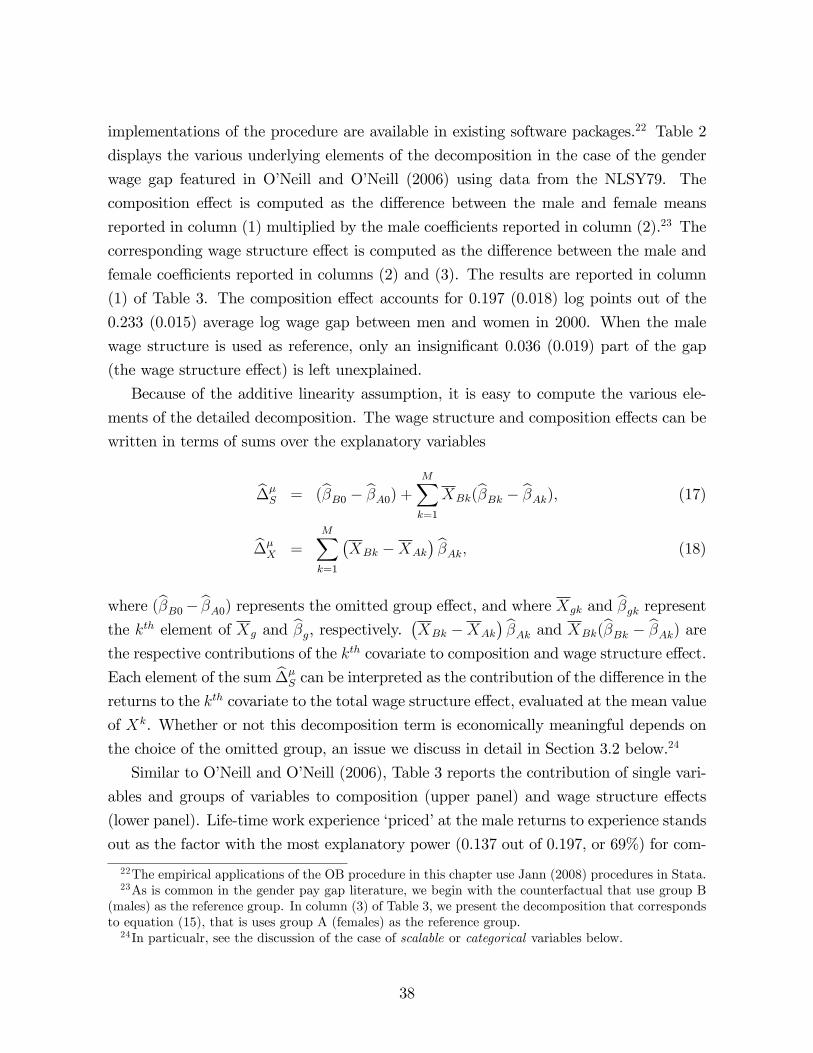
implementations of the procedure are available in existing software packages.22 Table 2

displays the various underlying elements of the decomposition in the case of the gender

wage gap featured in O�Neill and O�Neill (2006) using data from the NLSY79. The

composition e¤ect is computed as the di¤erence between the male and female means

reported in column (1) multiplied by the male coe¢ cients reported in column (2).23 The

corresponding wage structure e¤ect is computed as the di¤erence between the male and

female coe¢ cients reported in columns (2) and (3). The results are reported in column

(1) of Table 3. The composition e¤ect accounts for 0.197 (0.018) log points out of the

0.233 (0.015) average log wage gap between men and women in 2000. When the male

wage structure is used as reference, only an insigni�cant 0.036 (0.019) part of the gap

(the wage structure e¤ect) is left unexplained.

Because of the additive linearity assumption, it is easy to compute the various ele-

ments of the detailed decomposition. The wage structure and composition e¤ects can be

written in terms of sums over the explanatory variables

b��S = (b�B0 � b�A0) + MX

k=1

XBk(b�Bk � b�Ak); (17)

b��X =

MXk=1

�XBk �XAk

� b�Ak; (18)

where (b�B0� b�A0) represents the omitted group e¤ect, and where Xgk and b�gk representthe kth element of Xg and b�g, respectively. �XBk �XAk

� b�Ak and XBk(b�Bk � b�Ak) arethe respective contributions of the kth covariate to composition and wage structure e¤ect.

Each element of the sum b��S can be interpreted as the contribution of the di¤erence in the

returns to the kth covariate to the total wage structure e¤ect, evaluated at the mean value

of Xk. Whether or not this decomposition term is economically meaningful depends on

the choice of the omitted group, an issue we discuss in detail in Section 3.2 below.24

Similar to O�Neill and O�Neill (2006), Table 3 reports the contribution of single vari-

ables and groups of variables to composition (upper panel) and wage structure e¤ects

(lower panel). Life-time work experience �priced�at the male returns to experience stands

out as the factor with the most explanatory power (0.137 out of 0.197, or 69%) for com-

22The empirical applications of the OB procedure in this chapter use Jann (2008) procedures in Stata.23As is common in the gender pay gap literature, we begin with the counterfactual that use group B

(males) as the reference group. In column (3) of Table 3, we present the decomposition that correspondsto equation (15), that is uses group A (females) as the reference group.24In particualr, see the discussion of the case of scalable or categorical variables below.

38

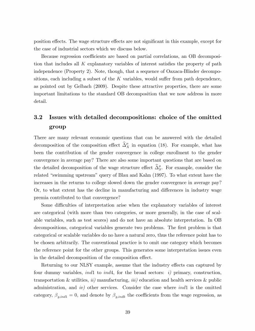
position e¤ects. The wage structure e¤ects are not signi�cant in this example, except for

the case of industrial sectors which we discuss below.

Because regression coe¢ cients are based on partial correlations, an OB decomposi-

tion that includes all K explanatory variables of interest satis�es the property of path

independence (Property 2). Note, though, that a sequence of Oaxaca-Blinder decompo-

sitions, each including a subset of the K variables, would su¤er from path dependence,

as pointed out by Gelbach (2009). Despite these attractive properties, there are some

important limitations to the standard OB decomposition that we now address in more

detail.

3.2 Issues with detailed decompositions: choice of the omitted

group

There are many relevant economic questions that can be answered with the detailed

decomposition of the composition e¤ect b��X in equation (18). For example, what has

been the contribution of the gender convergence in college enrollment to the gender

convergence in average pay? There are also some important questions that are based on

the detailed decomposition of the wage structure e¤ect b��S. For example, consider the

related �swimming upstream�query of Blau and Kahn (1997). To what extent have the

increases in the returns to college slowed down the gender convergence in average pay?

Or, to what extent has the decline in manufacturing and di¤erences in industry wage

premia contributed to that convergence?

Some di¢ culties of interpretation arise when the explanatory variables of interest

are categorical (with more than two categories, or more generally, in the case of scal-

able variables, such as test scores) and do not have an absolute interpretation. In OB

decompositions, categorical variables generate two problems. The �rst problem is that

categorical or scalable variables do no have a natural zero, thus the reference point has to

be chosen arbitrarily. The conventional practice is to omit one category which becomes

the reference point for the other groups. This generates some interpretation issues even

in the detailed decomposition of the composition e¤ect.

Returning to our NLSY example, assume that the industry e¤ects can captured by

four dummy variables, ind1 to ind4, for the broad sectors: i) primary, construction,

transportation & utilities, ii) manufacturing, iii) education and health services & public

administration, and iv) other services. Consider the case where ind1 is the omitted

category, �g;ind1 = 0, and denote by �g;indk the coe¢ cients from the wage regression, as

39

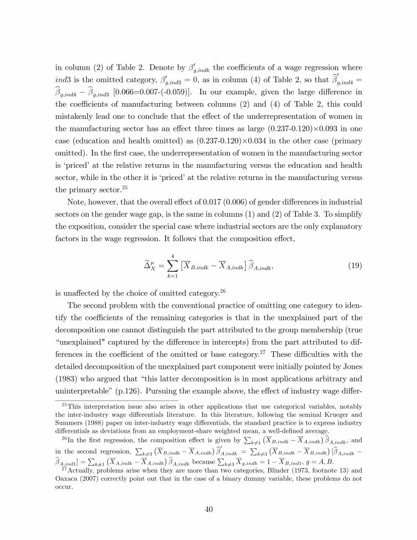
in column (2) of Table 2. Denote by �0g;indk the coe¢ cients of a wage regression where

ind3 is the omitted category, �0g;ind3 = 0, as in column (4) of Table 2, so that b�0g;ind4 =b�g;ind4 � b�g;ind3 [0.066=0.007-(-0.059)]. In our example, given the large di¤erence in

the coe¢ cients of manufacturing between columns (2) and (4) of Table 2, this could

mistakenly lead one to conclude that the e¤ect of the underrepresentation of women in

the manufacturing sector has an e¤ect three times as large (0.237-0.120)�0.093 in onecase (education and health omitted) as (0.237-0.120)�0.034 in the other case (primaryomitted). In the �rst case, the underrepresentation of women in the manufacturing sector

is �priced�at the relative returns in the manufacturing versus the education and health

sector, while in the other it is �priced�at the relative returns in the manufacturing versus

the primary sector.25

Note, however, that the overall e¤ect of 0.017 (0.006) of gender di¤erences in industrial

sectors on the gender wage gap, is the same in columns (1) and (2) of Table 3. To simplify

the exposition, consider the special case where industrial sectors are the only explanatory

factors in the wage regression. It follows that the composition e¤ect,

b��X =

4Xk=1

�XB;indk �XA;indk

� b�A;indk; (19)

is una¤ected by the choice of omitted category.26

The second problem with the conventional practice of omitting one category to iden-

tify the coe¢ cients of the remaining categories is that in the unexplained part of the

decomposition one cannot distinguish the part attributed to the group membership (true

�unexplained" captured by the di¤erence in intercepts) from the part attributed to dif-

ferences in the coe¢ cient of the omitted or base category.27 These di¢ culties with the

detailed decomposition of the unexplained part component were initially pointed by Jones

(1983) who argued that �this latter decomposition is in most applications arbitrary and

uninterpretable�(p.126). Pursuing the example above, the e¤ect of industry wage di¤er-

25This interpretation issue also arises in other applications that use categorical variables, notablythe inter-industry wage di¤erentials literature. In this literature, following the seminal Krueger andSummers (1988) paper on inter-industry wage di¤erentials, the standard practice is to express industrydi¤erentials as deviations from an employment-share weighted mean, a well-de�ned average.26In the �rst regression, the composition e¤ect is given by

Pk 6=1

�XB;indk �XA;indk

� b�A;indk, andin the second regression,

Pk 6=3

�XB;indk �XA;indk

� b�0A;indk = Pk 6=3

�XB;indk �XB;indk

�[b�A;indk �b�A;ind1] =Pk 6=1

�XA;indk �XA;indk

� b�A;indk because Pk 6=3Xg;indk = 1�XB;ind1, g = A;B.27Actually, problems arise when they are more than two categories, Blinder (1973, footnote 13) and

Oaxaca (2007) correctly point out that in the case of a binary dummy variable, these problems do notoccur.

40

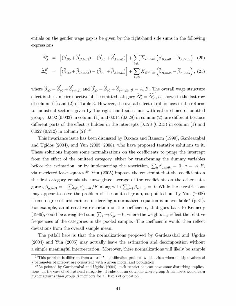
entials on the gender wage gap is be given by the right-hand side sums in the following

expressions

b��S =

h(b�0B0 + b�0B;ind1)� (b�0A0 + b�0A;ind1)i+X

k 6=1

XB;indk

�b�B;indk � b�A;indk� (20)

c��S

0=

h(b�B0 + b�B;ind3)� (b�A0 + b�A;ind3)i+X

k 6=3

XB;indk

�b�0B;indk � b�0A;indk� ; (21)where b�g0 = b�0g0 + b�0g;ind1 and b�0g0 = b�g0 + b�g;ind3, g = A;B. The overall wage structuree¤ect is the same irrespective of the omitted category b��

S =c��S

0, as shown in the last row

of column (1) and (2) of Table 3. However, the overall e¤ect of di¤erences in the returns

to industrial sectors, given by the right hand side sums with either choice of omitted

group, -0.092 (0.033) in column (1) and 0.014 (0.028) in column (2), are di¤erent because

di¤erent parts of the e¤ect is hidden in the intercepts [0.128 (0.213) in column (1) and

0.022 (0.212) in column (2)].28

This invariance issue has been discussed by Oaxaca and Ransom (1999), Gardeazabal

and Ugidos (2004), and Yun (2005, 2008), who have proposed tentative solutions to it.

These solutions impose some normalizations on the coe¢ cients to purge the intercept

from the e¤ect of the omitted category, either by transforming the dummy variables

before the estimation, or by implementing the restriction,P

k �g;indk = 0, g = A;B,

via restricted least squares.29 Yun (2005) imposes the constraint that the coe¢ cient on

the �rst category equals the unweighted average of the coe¢ cients on the other cate-

gories, �g;ind1 = �P

k 6=1 �g;indk=K along withPK

k=1 �g;indk = 0. While these restrictions

may appear to solve the problem of the omitted group, as pointed out by Yun (2008)

�some degree of arbitrariness in deriving a normalized equation is unavoidable" (p.31).

For example, an alternative restriction on the coe¢ cients, that goes back to Kennedy

(1986), could be a weighted sum,P

k wk�gk = 0, where the weights wk re�ect the relative

frequencies of the categories in the pooled sample. The coe¢ cients would then re�ect

deviations from the overall sample mean.

The pitfall here is that the normalizations proposed by Gardeazabal and Ugidos

(2004) and Yun (2005) may actually leave the estimation and decomposition without

a simple meaningful interpretation. Moreover, these normalizations will likely be sample

28This problem is di¤erent from a �true" identi�cation problem which arises when multiple values ofa parameter of interest are consistent with a given model and population.29As pointed by Gardeazabal and Ugidos (2004), such restrictions can have some disturbing implica-

tions. In the case of educational categories, it rules out an outcome where group B members would earnhigher returns than group A members for all levels of education.

41

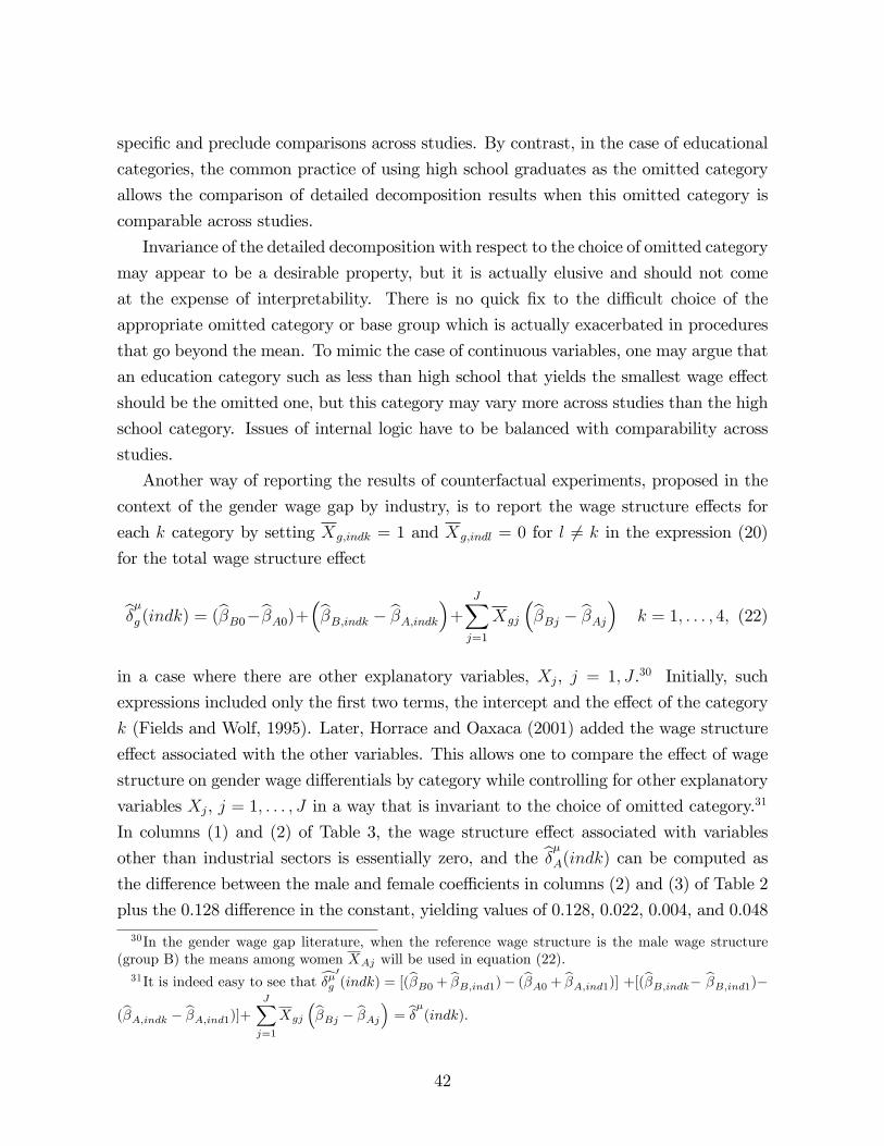
speci�c and preclude comparisons across studies. By contrast, in the case of educational

categories, the common practice of using high school graduates as the omitted category

allows the comparison of detailed decomposition results when this omitted category is

comparable across studies.

Invariance of the detailed decomposition with respect to the choice of omitted category

may appear to be a desirable property, but it is actually elusive and should not come

at the expense of interpretability. There is no quick �x to the di¢ cult choice of the

appropriate omitted category or base group which is actually exacerbated in procedures

that go beyond the mean. To mimic the case of continuous variables, one may argue that

an education category such as less than high school that yields the smallest wage e¤ect

should be the omitted one, but this category may vary more across studies than the high

school category. Issues of internal logic have to be balanced with comparability across

studies.

Another way of reporting the results of counterfactual experiments, proposed in the

context of the gender wage gap by industry, is to report the wage structure e¤ects for

each k category by setting Xg;indk = 1 and Xg;indl = 0 for l 6= k in the expression (20)for the total wage structure e¤ect

b��g (indk) = (b�B0�b�A0)+�b�B;indk � b�A;indk�+ JXj=1

Xgj

�b�Bj � b�Aj� k = 1; : : : ; 4; (22)

in a case where there are other explanatory variables, Xj, j = 1; J .30 Initially, such

expressions included only the �rst two terms, the intercept and the e¤ect of the category

k (Fields and Wolf, 1995). Later, Horrace and Oaxaca (2001) added the wage structure

e¤ect associated with the other variables. This allows one to compare the e¤ect of wage

structure on gender wage di¤erentials by category while controlling for other explanatory

variables Xj, j = 1; : : : ; J in a way that is invariant to the choice of omitted category.31

In columns (1) and (2) of Table 3, the wage structure e¤ect associated with variables

other than industrial sectors is essentially zero, and the b��A(indk) can be computed asthe di¤erence between the male and female coe¢ cients in columns (2) and (3) of Table 2

plus the 0.128 di¤erence in the constant, yielding values of 0.128, 0.022, 0.004, and 0.048

30In the gender wage gap literature, when the reference wage structure is the male wage structure(group B) the means among women XAj will be used in equation (22).31It is indeed easy to see that c��g 0(indk) = [(b�B0 + b�B;ind1)� (b�A0 + b�A;ind1)] +[(b�B;indk� b�B;ind1)�

(b�A;indk � b�A;ind1)]+ JXj=1

Xgj

�b�Bj � b�Aj� = b��(indk).42

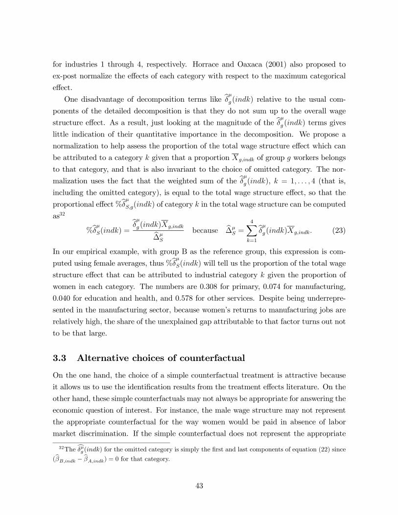
for industries 1 through 4, respectively. Horrace and Oaxaca (2001) also proposed to

ex-post normalize the e¤ects of each category with respect to the maximum categorical

e¤ect.

One disadvantage of decomposition terms like b��g (indk) relative to the usual com-ponents of the detailed decomposition is that they do not sum up to the overall wage

structure e¤ect. As a result, just looking at the magnitude of the b��g (indk) terms giveslittle indication of their quantitative importance in the decomposition. We propose a

normalization to help assess the proportion of the total wage structure e¤ect which can

be attributed to a category k given that a proportion Xg;indk of group g workers belongs

to that category, and that is also invariant to the choice of omitted category. The nor-

malization uses the fact that the weighted sum of the b��g (indk), k = 1; : : : ; 4 (that is,

including the omitted category), is equal to the total wage structure e¤ect, so that the

proportional e¤ect%b��S;g(indk) of category k in the total wage structure can be computedas32

%b��S(indk) = b��g (indk)Xg;indkb��S

because b��S =

4Xk=1

b��g (indk)Xg;indk: (23)

In our empirical example, with group B as the reference group, this expression is com-

puted using female averages, thus %b��S(indk) will tell us the proportion of the total wagestructure e¤ect that can be attributed to industrial category k given the proportion of

women in each category. The numbers are 0.308 for primary, 0.074 for manufacturing,

0.040 for education and health, and 0.578 for other services. Despite being underrepre-

sented in the manufacturing sector, because women�s returns to manufacturing jobs are

relatively high, the share of the unexplained gap attributable to that factor turns out not

to be that large.

3.3 Alternative choices of counterfactual

On the one hand, the choice of a simple counterfactual treatment is attractive because

it allows us to use the identi�cation results from the treatment e¤ects literature. On the

other hand, these simple counterfactuals may not always be appropriate for answering the

economic question of interest. For instance, the male wage structure may not represent

the appropriate counterfactual for the way women would be paid in absence of labor

market discrimination. If the simple counterfactual does not represent the appropriate

32The c��g (indk) for the omitted category is simply the �rst and last components of equation (22) since(b�B;indk � b�A;indk) = 0 for that category.

43

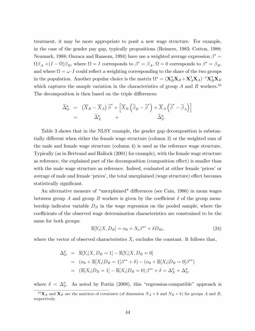
treatment, it may be more appropriate to posit a new wage structure. For example,

in the case of the gender pay gap, typically propositions (Reimers, 1983; Cotton, 1988;

Neumark, 1988; Oaxaca and Ransom, 1994) have use a weighted average expression �� =

�A +(I � )�B, where = I corresponds to �� = �A, = 0 corresponds to �� = �B,and where = ! �I could re�ect a weighting corresponding to the share of the two groupsin the population. Another popular choice is the matrix � = (X|

BXB+X|AXA)

�1X|BXB

which captures the sample variation in the characteristics of group A and B workers.33

The decomposition is then based on the triple di¤erences:

b��O =

�XB �XA

� b�� + hXB

�b�B � b���+XA

�b�� � b�A�i= b��

X + b��S:

Table 3 shows that in the NLSY example, the gender gap decomposition is substan-

tially di¤erent when either the female wage structure (column 3) or the weighted sum of

the male and female wage structure (column 4) is used as the reference wage structure.

Typically (as in Bertrand and Hallock (2001) for example), with the female wage structure

as reference, the explained part of the decomposition (composition e¤ect) is smaller than

with the male wage structure as reference. Indeed, evaluated at either female �prices�or

average of male and female �prices�, the total unexplained (wage structure) e¤ect becomes

statistically signi�cant.

An alternative measure of �unexplained" di¤erences (see Cain, 1986) in mean wages

between group A and group B workers is given by the coe¢ cient � of the group mem-

bership indicator variable DB in the wage regression on the pooled sample, where the

coe¢ cients of the observed wage determination characteristics are constrained to be the

same for both groups:

E[YijX;DB] = �0 +Xi��� + �DBi; (24)

where the vector of observed characteristics Xi excludes the constant. It follows that,

��O = E[YijX;DB = 1]� E[YijX;DB = 0]= (�0 + E[XijDB = 1]�

�� + �)� (�0 + E[XijDB = 0]���)

= (E[XijDB = 1]� E[XijDB = 0) ��� + � = ��

X +��S;

where � = ��S. As noted by Fortin (2008), this �regression-compatible� approach is

33XA and XB are the matrices of covariates (of dimension NA � k and NB � k) for groups A and B,respectively.

44

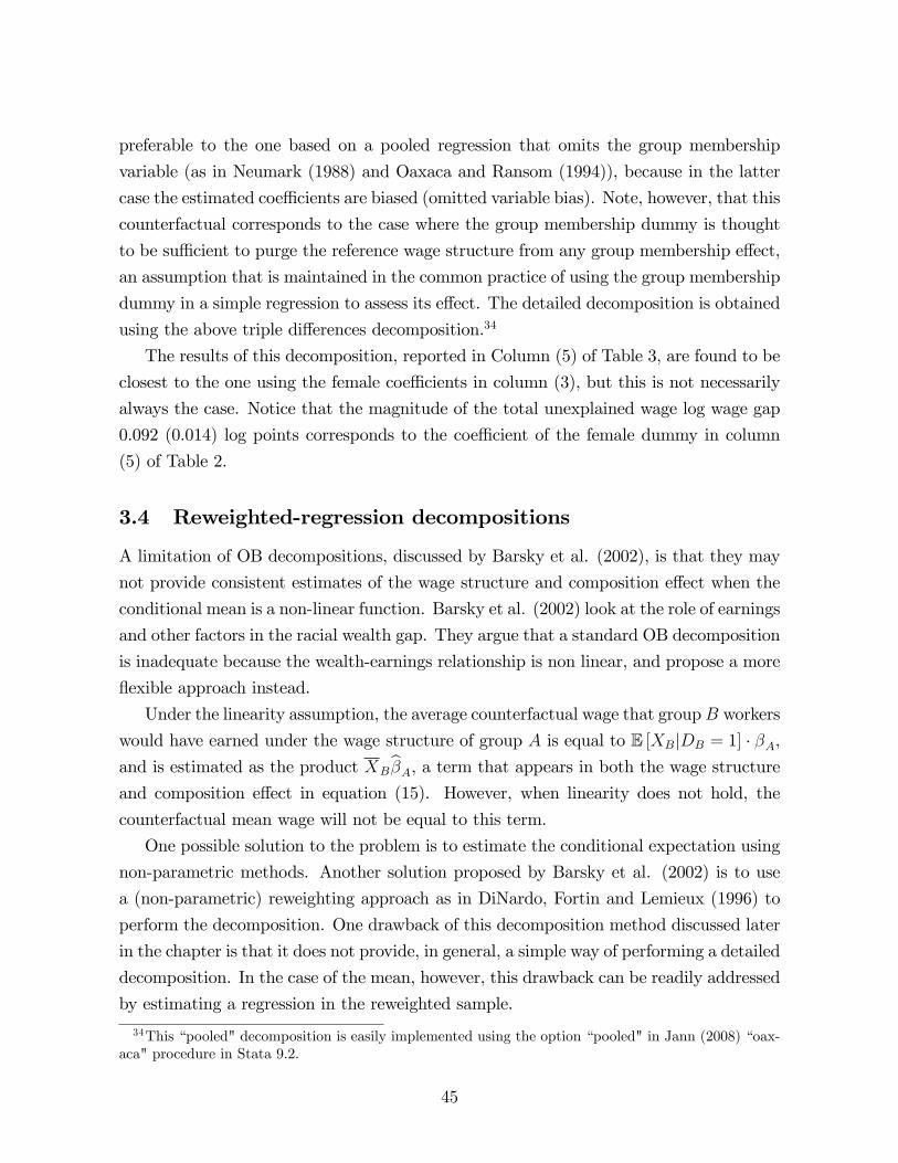
preferable to the one based on a pooled regression that omits the group membership

variable (as in Neumark (1988) and Oaxaca and Ransom (1994)), because in the latter

case the estimated coe¢ cients are biased (omitted variable bias). Note, however, that this

counterfactual corresponds to the case where the group membership dummy is thought

to be su¢ cient to purge the reference wage structure from any group membership e¤ect,

an assumption that is maintained in the common practice of using the group membership

dummy in a simple regression to assess its e¤ect. The detailed decomposition is obtained

using the above triple di¤erences decomposition.34

The results of this decomposition, reported in Column (5) of Table 3, are found to be

closest to the one using the female coe¢ cients in column (3), but this is not necessarily

always the case. Notice that the magnitude of the total unexplained wage log wage gap

0.092 (0.014) log points corresponds to the coe¢ cient of the female dummy in column

(5) of Table 2.

3.4 Reweighted-regression decompositions

A limitation of OB decompositions, discussed by Barsky et al. (2002), is that they may

not provide consistent estimates of the wage structure and composition e¤ect when the

conditional mean is a non-linear function. Barsky et al. (2002) look at the role of earnings

and other factors in the racial wealth gap. They argue that a standard OB decomposition

is inadequate because the wealth-earnings relationship is non linear, and propose a more

�exible approach instead.

Under the linearity assumption, the average counterfactual wage that groupB workers

would have earned under the wage structure of group A is equal to E [XBjDB = 1] � �A,and is estimated as the product XB

b�A, a term that appears in both the wage structure

and composition e¤ect in equation (15). However, when linearity does not hold, the

counterfactual mean wage will not be equal to this term.

One possible solution to the problem is to estimate the conditional expectation using

non-parametric methods. Another solution proposed by Barsky et al. (2002) is to use

a (non-parametric) reweighting approach as in DiNardo, Fortin and Lemieux (1996) to

perform the decomposition. One drawback of this decomposition method discussed later

in the chapter is that it does not provide, in general, a simple way of performing a detailed

decomposition. In the case of the mean, however, this drawback can be readily addressed

by estimating a regression in the reweighted sample.

34This �pooled" decomposition is easily implemented using the option �pooled" in Jann (2008) �oax-aca" procedure in Stata 9.2.

45

To see this, let (Xi) be the reweighting function, discussed in section 4.5, that

makes the characteristics of group A workers similar to those of group B workers. The

counterfactual coe¢ cients �CA and the counterfactual mean XC

A, are then estimated as:35

b�CA =

Xi2A

b(Xi) �Xi �X|i

!�1�Xi2A

b(Xi) � YAi �Xi

XC

A =Xi2A

b(Xi) �Xi;

where plim(XC

A) = plim(XB) = E(XjDB = 1).36 If the conditional expectation of Y

given X was linear, both the weighted and unweighted regressions would yield the same

consistent estimate of �A., i.e. we would have plim(b�CA) = plim(b�A) = �A. When the

conditional expectation is not linear, however, the weighted and unweighted estimates of

�A generally di¤er since OLS minimizes speci�cation errors over di¤erent samples.37

Consider the �reweighted-regression�decomposition of the overall wage gap b��O;R ,

where

b��O;R =

�XBb�B �XC

Ab�CA�+ �XC

Ab�CA �XA

b�A�= b��

S;R + b��X;R:

The composition e¤ect b��X;R can be divided into a pure composition e¤ect b��

X;p using

the wage structure of group A, and a component linking to the speci�cation error in the

35When considering covariates X, we use the subscript g to denote the group whose characteristicsare �adjusted" with reweighting.36We show in Section 4 that the reweighting factor (X) is de�ned as the ratio of the marginal

distributions of X for groups B and A, (X) = dFXB(X)=dFXA

(X). As a result, the reweighteddistribution of X for group A should be the same as the original distribution of X in group B. Thisimplies that the mean value of X in the reweighted sample, X

C

A, should be the same as the mean valueof X for group B, XB .37When the conditional expectation is non-linear, the OLS estimate of � can be interpreted as the one

which minimizes the square of the speci�cation error E(Y jX) � X� over the distribution of X. Sincethe expected value of the OLS estimate of � depends on the distribution of X, di¤erences in � over twosamples may either re�ect true underlying di¤erences in the conditional expectation (i.e. in the wagestructure), or �spurious� di¤erences linked to the fact that the distribution of X is di¤erent in thetwo samples. For example, if E(Y jX) is convex in X, the expected value of � will tend to grow as thedistribution of X shifts up, since the relationship between Y and X gets steeper as X becomes larger.

46

linear model, b��X;e:

b��X;R =

�XC

A �XA

� b�A +XC

A

hb�CA � b�Ai= b��

X;p + b��X;e:

The wage structure e¤ect can be written as

b��S;R = XB

�b�B � b�CA�+ �XB �XC

A

� c�CA= b��

S;p + b��S;e

and reduces to the �rst term b��S;p as the reweighting error b��

S;e goes to zero in large

samples (plim�XB �X

C

A

�= 0) plim(b��

S;e) = 0 ).

The reweighted-regression decomposition is similar to the usual OB decomposition

except for two small di¤erences. The �rst di¤erence is that the wage structure e¤ect is

based on a comparison between b�B and the weighted estimate b�CA instead of the usualunweighted estimate b�A. As discussed in Firpo, Fortin, and Lemieux (2007), this ensuresthat the di¤erence b�B � b�CA re�ects true underlying di¤erences in the wage structurefor group A and B, as opposed to a misspeci�cation error linked to the fact that the

underlying conditional expectation is non-linear. Note that is also useful to check whether

the reweighting error�XB �X

C

A

� b�CA is equal to zero (or close to zero), as it should bewhen the reweighting factor b(X) is consistently estimated.The other di¤erence relative to the OB decomposition is that the composition e¤ects

consists of a standard term�XC

A �XA

� b�A plus the speci�cation error XC

A

hb�CA � b�Ai.If the model was truly linear, the speci�cation error term would be equal to zero. Com-

puting the speci�cation error is important, therefore, for checking whether the linear

model is well speci�ed, and adjusting the composition e¤ect in the case where the linear

speci�cation is found to be inaccurate.

In the case where the conditional expectation E(YijXi; D = d) is estimated non-

parametrically, a whole di¤erent procedure would have to be used to separate the wage

structure into the contribution of each covariate. For instance, average derivative meth-

ods could be used to estimate an e¤ect akin to the � coe¢ cients used in standard decom-

positions. Unfortunately, these methods are di¢ cult to use in practice, and would not

be helpful in dividing up the composition e¤ect into the contribution of each individual

covariate.

On a related note, Kline (2009) points out that the standard OB decomposition can

47

be interpreted as a reweighting estimator where the weights have been linearized as a

function of the covariates. This suggests that the procedure may actually be more robust

to departures from linearity than what has been suggested in the existing literature.

Since the procedure is robust to these departures and remains the method of choice

when linearity holds, Kline (2009) points out that it is �doubly robust� in the sense of

Robins, Rotnizky, and Zhao (1994) and Egel, Graham, and Pinto (2009).

3.5 Extensions to limited dependent variable models

OB decompositions have been extended to cases where the outcome variable is not a

continuous variable. To mention a few examples, Gomulka and Stern (1990) study the

changes over time in labor force participation of women in the United Kingdom using

a probit model. Even and Macpherson (1990) decomposes the male-female di¤erence

in the average probability of unionization, while Doiron and Riddell (1994) propose a

decomposition of the gender gap in unionization rate based on a �rst order Taylor series

approximation of the probability of unionization. Fitzenberger et al. (2006) used a

probit model to decompose changes over time in the rate of unionization in West and

East Germany. Fairlie (1999; 2005) discuss the cases of the racial gaps in self-employment

and computer ownership. Bauer and Sinning (2008) discuss the more complicated cases of

a count data model, for example where the dependent variable is the number of cigarettes

smoked by men and women (Bauer, Göhlmann, and Sinning, 2007), and of the truncated

dependent variable, where for example the outcome of interest is hours of work.

In the case of a limited dependent variable Y , the conditional expectation of Y is

typically modelled as a non-linear function in X, E(YgjX; �g) = G(X; �g). For example,if Y is a dichotomous outcome variable (Y = 0; 1) and Y �g = X�g+�g is a latent variable

which is linear in X, it follows that E(YgjX; �g) = G(X�g) where G(�) is the PDF of �g.When �g follows a standard normal distribution, we have a standard probit model and

G(�) = �(�). More generally, under various assumptions regarding the functional formG and/or the distribution of the error terms �g, the models are estimated by maximum

likelihood.

Because E(YgjDg = 1) = E�E(YgjX; �g)jDg = 1

�= E

�G(X; �g)jDg = 1

�6= G

�E[Xj

Dg = 1]; �g�, the decomposition cannot simply be computed by plugging in the estimated

��s and the mean values of X�s, as in the standard OB decomposition. Counterfactual

conditional expectations have to be computed instead, and averaged across observa-

tions. For example, if group A is thought to be the reference group, E(YBjDA = 1) =

48

E [G(X; �B)jDA = 1] will be the counterfactual conditional expectation of YB that would

prevail if the coe¢ cients of the determinants of self-employment (for example) for group

B were the same as for group A. This involves computing predicted (i.e. expected) values

based on the estimated model for group B, G(X; �B), over all observations in group A,

and averaging over these predicted values.

The mean gap between group B and group A is then decomposed as follows

��O = E(YBjDB = 1)]� E(YAjDA = 1)

= E [G(X; �B)jDB = 1]� E [G(X; �A)jDA = 1]

=�E [G(X; �B)jDB = 1]� E [G(X; �A)jDB = 1]

�+�[E [G(X; �A)jDB = 1]� E [G(X; �A)jDA = 1]

�= ��

S + ��X ;

into a component that attributes di¤erences in the mean outcome variable to di¤erences

in the characteristics of the individuals, and a component that attributes these di¤erences

to di¤erences in the coe¢ cients.

The same di¢ cult issues in the appropriate choice of counterfactuals persist for more

general non-linear models. In addition, extra care has to be taken to verify that the

sample counterfactual conditional expectation lies within the bounds of the limited de-

pendent variable. For example, Fairlie (1999) checks that average self-employment for

Blacks predicted from the White coe¢ cients is not negative.

The non-linear decomposition may perform better than the linear alternative (linear

probability model, LPM) when the gap is located in the tails of the distribution or when

there are very large di¤erences in the explanatory variables, which e¤ects would remain

unbounded in a LPM. On the other hand, there are many challenges in the computation

of detailed decompositions for non-linear models. Because of non-linearity, the detailed

decomposition of the two components into the contribution of each variable, even if

the decomposition was linearized using marginal e¤ects, would not add up to the total.

Gomulka and Stern (1990) and Fairlie (2005) have proposed alternative methodologies

based on a series of counterfactuals, where the coe¢ cient of each variable is switched to

reference group values in sequence. In the latter cases, the decomposition will be sensitive

to the order of the decomposition, that is will be path dependent. We discuss these issues

further in the context of the decompositions of entire distributions in Section 5.

49

3.6 Statistical inference

OB decompositions have long been presented without standard errors. More recently,

Oaxaca and Ransom (1998), followed by Greene (2003, p. 53-54), have proposed approxi-

mate standard errors based the delta method under the assumption that the explanatory

variables were �xed.38 A more modern approach where, as above, (Y;X) are stochastic

was suggested and implemented by Jann (2005). In cases where the counterfactuals are

not a simple treatment, or where a non-linear estimator is used, boostrapping the entire

procedure may prove to be the practical alternative.

4 Going beyond the Mean - Distributional Methods

Developing new decomposition methods for distributional statistics other than the mean

has been an active research area over the last 15 years. In this section, we discuss a

number of procedures that have been suggested for decomposing general distributional

statistics. We focus on the case of the aggregate decomposition, though some of the

suggested methods can be extended to the case of the detailed decomposition, which

we discuss in section 5. We begin by looking at the simpler case of a variance decom-

position. The decomposition is obtained by extending the classic analysis of variance

approach (based on a between/within group approach) to a general case with covariates

X. We then turn to new approaches based on various �plugging in�methods such as

JMP�s residual imputation method and Machado and Mata (2005)�s conditional quantile

regression method. Finally, we discuss methods that focus on the estimation of counter-

factuals for the entire distribution. These methods are either based on reweighting or on

the estimation of the conditional distribution.

Most of this recent research was initially motivated by the dramatic growth in earnings

inequality in the United States. Prior to that episode, the literature was considering

particular summary measures of inequality such as the variance of logs and the Gini

coe¢ cient. For instance, Freeman (1980, 1984) looks at the variance of log wages in his

in�uential work on the e¤ect of unions on wage dispersion. This research establishes

that unions tend to reduce wage dispersion as measured by the variance of log wages.

Freeman shows that despite the inequality-enhancing e¤ect of unions on the between-

group component of inequality, the overall e¤ect of unions is to reduce inequality because

of the even larger e¤ect of unions on within-group inequality.

38This corresponds to an experimental setting where, for example, regression analysis was used toassess the impact of various soils and fertilizers (X) on agricultural yields Y .

50

One convenient feature of the variance is that it can be readily decomposed into

a within- and between-group component. Interestingly, related work in the inequality

literature shows that other measures such as the Gini or Theil coe¢ cient are also decom-

posable into a within and between group component.39

Note that the between vs. within decomposition is quite di¤erent in spirit from the

aggregate or detailed OB decomposition discussed in the previous section. There are

advantages and disadvantages to this alternative approach. On the positive side, looking

at between- and within-group e¤ects can help understand economic mechanisms, as in

the case of unions, or the sources of inequality growth (Juhn, Murphy, and Pierce, 1993).

On the negative side, the most important drawback of the between vs. within de-

composition is that it does not hold in the case of many other interesting inequality

measures such as the interquartile ranges, the probability density function, etc. This is a

major shortcoming since looking at what happens where in the distribution is important

for identifying the factors behind changes or di¤erences in distributions. Another draw-

back of the between vs. within approach is that it does not provide a straightforward

way of looking at the speci�c contribution of each covariate, i.e. to perform a detailed

decomposition. One �nal drawback is that with a rich enough set of covariates the num-

ber of possible groups becomes very large, and some parametric restrictions have to be

introduced to keep the estimation problem manageable.

In response to these drawbacks, a new set of approaches have been proposed for per-

forming aggregate decompositions on any distributional statistic. Some approaches such

as Juhn, Murphy, and Pierce (1993), Donald, Green, and Paarsch (2000), and Machado

and Mata (2005) can be viewed as extensions of the variance decomposition approach

where the whole conditional distribution (instead of just the conditional variance) are

estimated using parametric approaches. Others such as DiNardo, Fortin, and Lemieux

(1996) completely bypass the problem of estimating conditional distributions and are, as

such, closer cousins to estimators proposed in the program evaluation literature.

4.1 Variance decompositions

Before considering more general distributional statistics, it is useful the recall the steps

used to obtain the standard OB decomposition. The �rst step is to assume that the

conditional expectation of Y given X is linear, i.e. E(Y jX) = X�. This follows directlyfrom the linearity and zero conditional mean assumptions (Assumptions 10 and 11) in-

39See, for instance, Bourguignon (1979), Cowell (1980), and Shorrocks (1980, 1984).

51

troduced in Section 2. Using the law of conditional expectations, it then follows that

the unconditional mean is E(Y ) = E(E(Y jX)) = E(X)�. This particular property of themean is then used to compute the OB decomposition.

In light of this, it is natural to think of extending this type of procedure to the case

of the variance. Using the analysis of variance formula, the unconditional variance of Y

can be written as:40

V ar(Y ) = E[V ar(Y jX)] + E�[E(Y jX)� E(Y )]2

= E[V ar(Y jX)] + E

�[X� � E(X)�]2

= E[V ar(Y jX)] + �0V ar(X)�;

where the expectations are taken over the distribution of X. The �rst component of the

equation is the within-group component (also called residual variance), while the second

component is the between-group component (also called regression variance). Writing

V ar(Y jX;Dg = 1) �vg(X), g = A;B, we can write the di¤erence in variances across

groups B and A as

�VO = E [vB(X)jDB = 1]�E [vA(X)jDB = 0]+�

0BV ar [XjDB = 1] �B��0AV ar [XjDB = 0] �A:

A few manipulations yield �VO = �

VX +�

VS , where

�VX = fE [vA(X)jDB = 1]� E [vA(X)jDB = 0]g+�0A fV ar [XjDB = 1]� V ar [XjDB = 0]g �A

and

�VS = fE [vB(X)jDB = 1]� E [vA(X)jDB = 1]g+(�B � �A)

0V ar [XjDB = 1] (�B � �A):

While it is straightforward to estimate the regression coe¢ cients (�A and �B) and the

covariance matrices of the covariates (V ar [XjDB = 0] and V ar [XjDB = 1]), the within-

group (or residual) variance terms vA(X) and vB(X) also have to be estimated to compute

the decomposition.

Several approaches have been used in the literature to estimate vA(X) and vB(X).

The simplest possible approach is to assume that the error term is homoscedastic, in

which case vA(X) = �2A and vB(X) = �2B, and the two relevant variance parameters

can be estimated from the sampling variance of the error terms in the regressions. The

40See for example, Theorem B.4 in Greene (2003).

52

homoscedasticity assumption is very strong, however. When errors are heteroscedastic,

di¤erences between �2A and �2B can re�ect spurious composition e¤ects, in which case the

decomposition will attribute to the wage structure e¤ect (�VS ) what should really be a

composition e¤ect (�VX). Lemieux (2006b) has shown this was a major problem when

looking at changes in residual wage inequality in the United States since the late 1980s.

A simple way of capturing at least some of the relationship between the covariates

and the conditional variance is to compute the variance of residuals for a limited number

of subgroups of �cells�. For instance, Lemieux (2006b) shows estimates for 20 di¤erent

subgroups of workers (based on education and experience), while Card (1996) divides the

sample in �ve quintiles based on predicted wages Xb�.Finally, one could attempt to estimate a more general speci�cation for the condi-

tional variance by running a �second step�model for squared regression residual b�2 =�Y �Xb��2 on some speci�cation of the covariates. For example, assuming that vA(X) =X�, we can estimate estimate b� by running a regression of b�2 on X.41 We can then writethe two aggregate components of the variance decomposition as:

�VX = f(E [XjDB = 1]� E [XjDB = 0]) �Ag+�0A fV ar [XjDB = 1]� V ar [XjDB = 0]g �A

(25)

and

�VS = fE [XjDB = 1] (�B � �A)g+ (�B � �A)

0V ar [XjDB = 1] (�B � �A): (26)

Compared to the standard OB decomposition for the mean, which only requires es-

timating a (regression) model for the conditional mean, in the case of the variance, we

also need to estimate a model for the conditional variance. While this is quite feasi-

ble in practice, we can already see a number of challenges involved when decomposing

distributional parameters beyond the mean:

� The estimation is more involved since we need to estimate models for two, insteadof just one, conditional moment. Furthermore, little guidance is typically available

on �reasonable�speci�cations for the conditional variance. For instance, in the case

of wages, the Mincer equation provides a reasonably accurate and widely accepted

speci�cation for the conditional mean, while no such standard model is available

for the conditional variance.41Estimating these simple models of the conditional cross-sectional variance is a special case of the

large time-series literature on the estimation of auto-regressive conditional heteroskedasticity models(ARCH, GARCH, etc.).

53

� Computing the detailed decomposition is more complicated since the between-groupcomponent is a quadratic form in the ��s. This yields a number of interaction terms

that are di¢ cult to interpret.

Since the complexity of decomposition methods already increases for a distributional

measure as simple and convenient as the variance, this suggests these problems will be

compounded in the case of other distributional measures such as quantiles. Indeed, we

show in the next subsection that for quantiles, attempts at generalizing the approach

suggested here require estimating the entire conditional distribution of Y given X. This

is a more daunting estimation challenge, and we now discuss solutions that have been

suggested in the literature.

4.2 Going beyond the variance: general framework

An important limitation of summary measures of dispersion such as the variance, the

Gini coe¢ cient or the Theil coe¢ cient is that they provide little information regarding

what happens where in the distribution. This is an important shortcoming in the litera-

ture on changes in wage inequality where many important explanations of the observed

changes have speci�c implications for speci�c points of the distribution. For instance, the

minimum wage explanation suggested by DiNardo, Fortin, and Lemieux (1996) should

only a¤ects the bottom end of the distribution. At the other extreme, explanations based

on how top executives are compensated should only a¤ect the top of the distribution.

Other explanations based on de-unionization (Freeman, 1993, Card, 1992, and DiNardo,

Fortin, and Lemieux, 1996) and the computerization of �routine�jobs (Autor, Levy and

Murnane, 2003) tend to a¤ect the middle (or �lower middle�) of the distribution. As a

result, it is imperative to go beyond summary measures such as the variance to better

understand the sources of growing wage inequality.

Going beyond summary measures is also important in many other interesting eco-

nomic problems such the sources of the gender wage gap and the impact of social pro-

grams on labor supply.42 The most common approach for achieving this goal is to perform

a decomposition for various quantiles (or di¤erences between quantiles like the 90-10 gap)

of the distribution. Unfortunately, as we point out in the introduction, it is much more

di¢ cult to decompose quantiles than the mean or even the variance. The basic prob-

lem is that the law of iterated expectations does not hold in the case of quantiles, i.e.42See Albrecht, Björklund, and Vroman (2003) who look at whether there is a glass ceiling in female

earnings, and Bitler, Gelbach and Hoynes (2006) who study the distributional e¤ects of work incentiveprograms on labor supply.

54

Qg;� 6= EX [Qg;� (X)], where Qg;� , is the � th quantile of the (unconditional) distribution ofYg, and Qg;� (X) is the corresponding conditional quantile.

As it turns out, one (implicitly) needs to know the entire conditional distribution of

Yg given X given to compute Qg;� . To see this, note that

� = FYg(Qg;� ) = E[FYg jXg(Qg;� jX)] =ZFYg jXg(Qg;� jX)dFXg(X); g = A;B;

where FYg jXg(�) is the cumulative distribution of Y conditional on X in group g. Given

� , it is possible to implicitly use this equation to solve out for Qg;� . It is also clear that in

order to do so we need to know the conditional distribution function FYg jXg(�), as opposedto just the conditional mean and variance, as was the case for the variance. Estimating

an entire conditional distribution function for each value of (YgjX) is a di¢ cult problem.Various decomposition methods that we discuss in detail below suggest di¤erent ways of

handling this challenge.

But before covering them in detail, we recall the basic principles underlying these

methods. As in Section 2, we focus on cumulative distributions since any standard

distribution statistic, such as a quantile, can be directly computed from the cumulative

distribution. For instance, quantiles of the counterfactual distribution can be obtained

by inverting FY CA : QCA;� = F

�1Y CA(�):

For the sake of presentational simplicity, we introduce a simpli�ed notation relative

to Section 2. We use FXg instead of FXjDg to represent the marginal distribution of X,

and FYg jXg to represent FYg jX;Dg the conditional distributions, for g = A;B introduced

in equation (4). We use the shorthand FY CA instead of FY CA :X=XjDB to represent the

key counterfactual distribution of interest introduced in equation (5), which mixes the

distribution of characteristics of group B with the wage structure from group A:

FY CA (y) =

ZFYAjXA(yjX)dFXB(X): (27)

Three general approaches have been suggested in the decomposition literature for

estimating the counterfactual distribution FY CA (y). A �rst general approach, initially

suggested by Juhn, Murphy and Pierce (1993), replaces each value of YB for group B

with a counterfactual value of Y CA = g(YB; X), where g(�; �) is an imputation function.The idea is to replace YB from group B with a counterfactual value of Y CA that holds the

same rank in the conditional distribution FYAjXA(�j�) as it did in the original distributionof YB. As we discussed in Section 2.2.3, this is done in practice using a residual imputation

55

procedure. Machado and Mata (2005) and Autor, Katz, and Kearney (2005) have later

suggested other approaches, based on conditional quantile regressions, to transform a

wage observation YB into a counterfactual observation Y CA .

A second approach proposed by DiNardo, Fortin, and Lemieux (1996) [DFL] is based

on the following manipulation of equation (27):

FY CA (y) =

ZFYAjXA(yjX)(X)dFXA(X); (28)

where (X) =dFXB(X)=dFXA(X) is a reweighting factor. This makes it clear that the

counterfactual distribution FY CA (�) is simply a reweighted version of the distributionFYA(�). The reweighting factor is a simple function of X that can be easily estimated

using standard methods such as a logit or probit. The basic idea of the DFL approach is

to start with group A, and then replace the distribution of X of group A (FXA(�)) withthe distribution of X of group B (FXB(�)) using the reweighting factor (�).The third set of approaches also works with equation (27) starting with group B, and

then replacing the conditional distribution FYB jXB(Y jX) with FYAjXA(Y jX). Doing sois more involved, from an estimation point of view, than following the DFL approach.

The problem is that the conditional distributions depend on both X and y, while the

reweighting factor (X) only depends on X.

Under this third set of approaches, one needs to directly estimate the conditional

distribution FY jX(yjX). Parametric approaches for doing so were suggested by Don-ald, Green, and Paarsch (2000) who used a hazard model approach, and Fortin and

Lemieux (1998) who suggested estimating an ordered probit. More recently, Cher-

nozhukov, Fernandez-Val, and Melly (2009) suggest estimating distributional regressions

(e.g. a logit, for each value of y). In all cases, the idea is to replace the conditional

distribution for group B, FYB jXB(yjX), with an estimate of the conditional distributionFYAjXA(yjX) obtained using one of these methods.In the next subsections, we discuss how these various approaches can be implemented.

We also present some results regarding their statistical properties, and address compu-

tational issues linked to their implementation.

4.3 Residual Imputation Approach: JMP

ProcedureAs we explain above, Juhn, Murphy, and Pierce (1993) propose an imputation ap-

proach where the wage YB from group B is replaced by a counterfactual wage Y CA where

56

both the returns to observables and unobservables are set to be as in group A. The im-

plementation of this procedure is divided in two steps. First, unobservables are replaced

by counterfactual unobservables, as in equation (9). Second, counterfactual returns to

observables are also imputed, as in equation (12).43

Under the assumption of additive linearity (Assumption 10), the original wage equa-

tion for individual i from group B,

YBi = Xi�B + �Bi where �Bi = hB("i)

allows the returns to unobservables to be group-speci�c. Under the assumption of rank

preservation (14), the �rst counterfactual is computed as

Y C;2Ai = Xi�B + �C;2Ai ; (29)

where

�C;2Ai = F�1�AjX(�Bi(xi); xi);

and �Bi(xi) is the conditional rank of �Bi in the distribution of residuals for group B

(�Bi(xi) = F�B jX (�BijX = xi)). A second counterfactual is then obtained by also replac-

ing the returns to observable characteristics �B with �A

Y C;3Ai = Xi�A + �C;2Ai :

Under the assumptions of linearity and rank preservation, this counterfactual wage

should the same as Y CAi, the counterfactual wage obtained by replacing the wage structure

mB(�) with mA(�).In practice, it is straightforward to estimate �A and �B using OLS under the as-

sumptions of linearity and zero conditional mean. It is much less clear, however, how to

perform the residual imputation procedure described above. Under the strong assump-

tion that the regression residuals �g are independent of X, it follows that

�C;2Ai = F�1�A(�Bi):

Under this independence assumption, one simply needs to compute the rank of the resid-

43Juhn, Murphy, and Pierce (1993) actually consider multiple time periods and proposed an additionalcounterfactual where the returns to observables are set to their mean across time periods, a complexcounterfactual treatment.

57

ual �Bi in the marginal distribution (distribution over the whole sample) of residuals for

group B, and then pick the corresponding residuals in the marginal distribution of resid-

uals for group A. If �Bi is at the 70th percentile of the distribution of residuals of group B

(�Bi = :7), then �C;2Ai will simply be the 70

th percentile of the distribution of residuals for

group A. In practice, most applications of the JMP procedure use this strong assump-

tion of independence because there is little guidance as to how a conditional imputation

procedure could be used instead.

LimitationsSince independence of regression residuals is unrealistic, a more accurate implemen-

tation of JMP would require deciding how to condition on X when performing the impu-

tation procedure. If X consists of a limited number of groups or �cells�, then one could

perform the imputation within each of these groups. In general, however, it is di¢ cult

to know how to implement this ranking/imputation procedure in more general cases. As

a result, other procedures such as the quantile method of Machado and Mata (2005) are

increasingly being used as an alternative to JMP.

Another limitation of the JMP procedure is that there is no natural way of extending

it to the case of the detailed decomposition for the composition e¤ect.

AdvantagesOne advantage of the two-step procedure is that it provides a way of separating

the between- and within-group components, as in a variance decomposition. This plays

an important role in the inequality literature, since JMP concluded that most of the

inequality growth from the 1960s to the 1980s was linked to the residual inequality

component.

It is not clear, however, what is meant by between- and within-group components in

the case of distributional measures like the 90-10 gap that are not decomposable. A better

way of justifying JMP is that Y = X� + � represents a structural model where X are

observed skills, while � represents unobserved skills. One can then perform simulation

exercises asking what happens to the distribution when one either replaces returns to

observed or unobserved skills (see also Section 2.2.3).

This economic interpretation also requires, however, some fairly strong assumptions.

The two most important assumptions are the linearity of the model (assumption 10,

mg (Xi; "i) = Xi�g + �gi) and rank preservation (assumption 14). While linearity can be

viewed as a useful approximation, rank preservation is much stronger since it means that

someone with the same unobserved skills would be in the exact same position, conditional

on X, in either group A or B. Just adding measurement error to the model would result

58

in a violation of rank preservation.

Finally, if one is willing to interpret a simple regression as a decomposition between

observed and unobserved skills, this can be combined with methods other than JMP.

For instance, DFL perform regression adjustments to illustrate the e¤ects of supply and

demand factors on wages.44

4.4 Methods based on conditional quantiles

ProcedureLike JMP, Machado and Mata (2005, MM from hereinafter) propose a procedure

based on transforming a wage observation YB into a counterfactual observation Y CA .

The main advantage relative to JMP is that their estimation procedure based on quan-

tile regressions (Koenker and Bassett, 1978) provides an explicit way of estimating the

(inverse) conditional distribution function F�1YAjXA(�; �) in the transformation g(Y;X) =F�1YAjXA(FYB jXB(Y jX); X). One important di¤erence, however, is that instead of trans-forming each actual observation of YBi into a counterfactual Y CAi, MM use a simulation

approach where quantiles are drawn at random.

More speci�cally, since

Y CA = F�1YAjXA(FYB jXB(Y jX); X);

and �B(Y jX) =FYB jXB(Y jX) follows a uniform distribution, one can think of doing the

following:

1. Draw a simulated value � s from a uniform distribution s = 1; : : : ; S.

2. Estimate a linear quantile regression for the � ths quantile, and use the estimated

result to predict simulated values of both YBs and Y CAs.45 The reason for using quantile

regressions is that:

Y CAs=F�1YAjXA(� s; X) and YBs=F

�1YB jXB(� s; X);

where F�1YAjXA(�; �) and F�1YB jXB(�; �) are the conditional quantile functions for the �

ths quan-

tile in group A and B, respectively.

3. Compare the simulated distributions of YBs and Y CAs to obtain measures of the wage

44See also Lemieux (2002).45For each random draw s, MM also draw a vector of covariatesXs from the observed data and perform

the prediction for this value only. Melly (2005) discusses more e¢ cient ways of computing dsitributionsusing this conditional quantile regression approach.

59

structure e¤ect. The composition e¤ect is computed as the complement to the overall

di¤erence.

A key implementation question is how to specify the functional forms for the con-

ditional quantile functions. MM suggest a linear speci�cation in the X that can be

estimated using quantile regression methods. The conditional quantile regression models

can be written as:

Qg;� (Y jX)=F�1Yg jXg(� ;X) = X�g;� ; g = A;B

Table 4 reports in the top panel the results of the Machado-Mata procedure applied to

our gender gap example using the male wage structure as reference.46 It shows that the

median gender log wage gap in the central column gives almost the same results for the

aggregate decomposition as the OB mean gender log wage gap decomposition displayed

in column (1) of Table 3. Going across the columns to compare quantile e¤ects shows

that gender di¤erences in characteristics are much more important at the bottom (10th

centile) than at the top (90th centile) of the wage distribution. Indeed, some signi�cant

wage structure e¤ects emerge at the 90th percentile.

LimitationsThis decomposition method is computationally demanding, and becomes quite cum-

bersome for data sets numbering more than a few thousand observations. Bootstrapping

quantile regressions for sizeable number of quantiles � (100 would be a minimum) is

computationally tedious with large data sets. The implementation of the procedure can

be simpli�ed by estimating a large number of quantile regressions (say 99, one for each

percentile from 1 to 99) instead of drawing values of � s at random.47

Another limitation is that the linear speci�cation is restrictive and �nding the correct

functional for the conditional quantile regressions can be very tedious. For instance, if

there is a spike at the minimum wage in the wage distribution, this will result in �at

spots in quantile regressions that would have to be captured with spline functions with

knots that depend on X. Accurately describing simple distribution with mass points (as

is commonly observed in wage data) can, therefore, be quite di¢ cult to do using quantile

regressions.

As pointed out by Chernozhukov, Fernandez-Val, and Melly (2009), it is not very

46The estimates were computed with Melly�s implementation �rqdeco�in Stata.47See Melly (2005) for a detailed description of this alternative procedure. Gosling, Machin, and

Meghir (2000) and Autor, Katz, and Kearney (2005) also use a similar idea in their empirical applicationsto changes in the distribution of wages over time.

60

natural to estimate inverse conditional distribution functions (quantile regressions) when

the main goal of counterfactual exercises is to replace the conditional distribution function

FYB jXB with FYAjXA to obtain equation (27). Chernozhukov, Fernandez-Val, and Melly

(2009) suggest instead to estimate directly distributional regression models for FY jX(�; �),which is a more direct way of approaching the problem.

AdvantagesOne advantage of the MM approach is that it provides a natural way of performing

a detailed decomposition for the wage structure component. The idea is to successively

replace the elements of �B;� by those of �A;� when performing the simulations, keeping

in mind that this type of detailed decomposition is path dependent. Unfortunately, the

MM does not provide a way of performing the detailed decomposition for the composition

e¤ect.48 This is a major drawback since the detailed decomposition of the composition

e¤ects is always clearly interpretable, while the detailed decomposition of the wage struc-

ture e¤ect arbitrarily depends on the choice of the omitted group.

4.5 Reweighting methods

ProcedureAs we mention in Section 4.2, another way of estimating the counterfactual distribu-

tion FY CA (�) is to replace the marginal distribution of X for group A with the marginal

distribution of X for group B using a reweighting factor (X). This idea was �rst in-

troduced in the decomposition literature by DiNardo, Fortin and Lemieux [DFL] (1996).

While DFL focus on the estimation of counterfactual densities in their empirical appli-

cation, the method is easily applicable to any distributional statistic.

In practice, the DFL reweighting method is similar to the propensity score reweighting

method commonly used in the program evaluation literature (see Hirano, Imbens, and

Ridder, 2003). For instance, in DFL�s application to changes in wage inequality in the

United States, time is viewed as a state variable, or in the context of the treatment e¤ects

literature as a treatment.49 The impact of a particular factor or set of factors on changes

in the wage distribution over time is constructed by considering the counterfactual state

48Machado and Mata (2005) suggest computing the detailed decomposition for the composition e¤ectusing an unconditional reweighting procedure. This is invalid as a way of performing the decompositionfor the same reason that a OB decomposition would be invalid if the � coe¢ cient used for one covari-ate was estimated without controlling for the other covariates. We propose a conditional reweightingprocedure in the next section that deals adequately with this issue.49This view of course makes more sense when some policy or other change has taken place over time

(see Biewen (2001).

61

of the world where the distribution of this factor remained �xed in time, maintaining the

assumption 6 of invariance of the conditional distribution. Note that by contrast with the

notation of this chapter, in DFL, time period 1 is used as reference group.50 The choice

of period 0 or period 1 as the reference group is analogous to the choice of whether the

female or the male wage structure should be the reference wage structure in the analysis

of the gender wage gap and is expected to yield di¤erent results in most cases.

In DFL, manipulations of the wage distributions, computed through reweighting,

are applied to non-parametric estimates of the wage density, which can be particularly

useful when local distortions, from minimum wage e¤ects for example, are at play. To be

consistent with the rest of this section, however, we focus our discussion on the cumulative

distribution instead of the density. The key counterfactual distribution of interest, shown

in equation (27) (distribution of wages that would prevail for workers in group A if they

had the distribution of characteristics of group B) is constructed, as shown in equation

(28), using the reweighting factor

(X) =dFXB(X)

dFXA(X):

Although the reweighting factor is the ratio of two multivariate marginal distribu-

tion functions (of the covariates X), this expression can be simpli�ed using Bayes�rule.

Remembering that Bayes�rule states that

P (BijA) = P (AjBi) � P (Bi)=Xj

P (AjBj) � P (Bj):

We have

Pr(XjDB = 1) =Pr(DB = 1jX) � dF (X)RxPr(DB = 1jX) � dF (X)

=Pr(DB = 1jX)Pr(DB = 1)

and a similar expression for DB = 0. Since dFXA(X) = Pr(XjDB = 0) and dFXB(X) =

Pr(XjDB = 1), the reweighting factor that keeps all conditioning variables as in period

0 becomes

(X) =Pr(XjDB = 1)

Pr(XjDB = 0)=Pr(DB = 1jX)=Pr(DB = 1)

Pr(DB = 0jX)=Pr(DB = 0):

The reweighting factor can be easily computed by estimating a probability model

for Pr(DB = 1jX), and using the predicted probabilities to compute a value b(X) foreach observation. DFL suggest estimating a �exible logit or probit model, while Hirano,

50On the other hand, by analogy with the treatment e¤ects literature, Firpo, Fortin, and Lemieux(2007) use time period 0 as the reference group.

62

Imbens, and Ridder propose to use a non-parametric logit model.51

The reweighting decomposition procedure can be implemented in practice as follows:

1. Pool the data for group A and B and run a logit or probit model for the probability

of belonging to group B:

Pr(DB=1jX) = 1� Pr(DB=0jX) = 1� Pr(" > �h(X)�) = �(�h(X)�) (30)

where �() is either a normal or logit link function, and h(X) is a polynomial in X.

2. Estimate the reweighting factor b(X) for observations in group A using the pre-dicted probability of belonging to group B (cPr(DB = 1jX)) and A (cPr(DB = 0jX) =1 � cPr(DB = 1jX)), and the sample proportions in group B (cPr(DB = 1)) and A

(cPr(DB = 0)): b(X) = cPr(DB = 1jX)=cPr(DB = 1)cPr(DB = 0jX)=cPr(DB = 0):

3. Compute the counterfactual statistic of interest using observations from the group

A sample reweighted using b(X).In DFL, the main object of interest is the probability density function, which is

estimated using kernel density methods. The density for group A and the counterfactual

density can be estimated as follows using kernel density methods, whereK(:) is the kernel

function:52

bfYA(y) =1

h �NA

Xi2A

K

�Yi � yh

�;

bfY CA (y) =1

h �NA

Xi2A

b(Xi) �K�Yi � yh

�:

Consider the density function for group A, fYA(y), and the counterfactual density fY CA (y).

The composition e¤ect in a decomposition of densities is:

�f(y)X = fY CA (y)� fYA(y): (31)

Various statistics from the wage distribution, such as the 10th, 50th, and 90th per-

centile, or the variance, Gini, or Theil coe¢ cients can be computed either from the

51The estimator suggested by Hirano, Imbens, and Ridder (2003) is a series estimator applied to thecase of a logit model. The idea is to add increasingly higher order polynomial terms in the covariatesas the size of the sample increases. Importantly, they also show that this approach yields an e¢ cientestimate of the treatment e¤ect.52The two most popular kernel functions are the Gaussian and the Epanechnikov kernel.

63

counterfactual density or the counterfactual distribution using the reweighting factor.

The latter procedure is easier to use as it simply involves computing (weighted) statis-

tics using standard computer packages. For example, the counterfactual variance can be

computed as: dV arY CA = 1

NA

Xi2A

b(Xi) ��Yi � b�Y CA �2 ;

where the counterfactual mean b�Y CA is:

b�Y CA = 1

NA

Xi2A

b(Xi) � Yi:

For the 90-10, 90-50, and 50-10 wage di¤erentials, the sought-after contributions to

changes in inequality are computed as di¤erences in the composition e¤ects, for example,

�90�10X = [QCA;:9 �QA;:9]� [QCA;:1 �QA;:1]: (32)

Table 5 presents, in panel A, the results of a DFL decomposition of changes over time

in male wage inequality using large samples from combined MORG-CPS data as in Firpo,

Fortin, and Lemieux (2007). In this decomposition, the counterfactual distribution of

wages in 1983/85 is constructed by reweighting the characteristics of workers in 1983/85

(time period 0) so that they look like those of 2003/05 (time period 1) workers, holding

the conditional distribution of wages in 1983/05 �xed.53 The results of the aggregate

decomposition, reported in the �rst three rows of Table 5, show that composition e¤ects

play a large role in changes in overall wage inequality, as measured by the 90-10 log

wage di¤erential or the variance of log wages. But the wage structure e¤ects are more

important when looking for increases at the top of the wage distribution, as measured

by the 90-50 log wage di¤erential, or decreases in the bottom, as measured by the 50-10

log wage di¤erential.

AdvantagesThe main advantage of the reweighting approach is its simplicity. The aggregate

decomposition for any distributional statistics is easily computed by running a single

probability model (logit or probit) and using standard packages to compute distributional

statistics with b(Xi) as weight.

53By contrast, in the original DiNardo, Fortin, and Lemieux (1996) decomposition, workers in 1988(time period 1) were reweighed to look like workers in 1979 (time period 0). The counterfactual distrib-ution of wages was asking what would the distribution of wages look like if the workers�characteristicshad remained at 1979 levels.

64

Another more methodological advantage is that formal results from Hirano, Imbens,

and Ridder (2003) and Firpo (2007, 2010) establish the e¢ ciency of this estimation

method. Note that although it is possible to compute analytically the standard errors

of the di¤erent elements of the decomposition obtained by reweighting, it is simpler in

most cases to conduct inference by bootstrapping.54

For these two reasons, we recommend the reweighting approach as the method of

choice for computing the aggregate decomposition. This recommendation even applies

in the simple case of the mean decomposition. As pointed out by Barsky et al. (2002), a

standard OB decomposition based on a linear regression model will yield biased estimates

of the decomposition terms when the underlying conditional expectation of Y given X is

non-linear (see Section 3.4). They suggest using a reweighting approach as an alternative,

and the results of Hirano, Imbens, and Ridder (2003) can be used to show that the

resulting decomposition is e¢ cient.

LimitationsA�rst limitation of the reweighting method is that it is not straightforwardly extended

to the case of the detailed decomposition. One exception is the case of binary covariates

where it is relatively easily to compute the corresponding element of the decomposition.

For instance, in the case of the union status (a binary covariate), DFL show how to

compute the component of the composition corresponding to this particular covariate. It

also relatively easy to compute the corresponding element of the wage structure e¤ect. We

discuss in Section 5 other options that can be used in the case of non-binary covariates.

As in the program evaluation literature, reweighting can have some undesirable prop-

erties in small samples when there is a problem of common support. The problem is

that the estimated value of (X) becomes very large when Pr(DB = 1jX) gets closeto 1. While lack of common support is a problem for any decomposition procedure,

Frolich (2004) �nds that reweighting estimators perform particularly poorly in this con-

text, though Busso, DiNardo, and McCrary (2009) reach the opposite conclusion using

a di¤erent simulation experiment.55

Finally, even in cases where a pure reweighting approach has some limitations, there

may be gains in combining reweighting with other approaches. For instance, we discuss

54The analytical standard errors have to take account of the fact that the logit or probit model usedto construct the reweighting factor is estimated. Firpo, Fortin and Lemieux (2007) show how to performthis adjustment. In practice, however, it is generally simpler to bootstrap the whole estimation procedure(both the estimation of the logit/probit to construct the weights and the computation of the variouselements of the decomposition).55In principle, other popular methods in the program evaluation literature such as matching could be

used instead of reweighting.

65

in the next section how reweighting can be used to improve a decomposition based on

the RIF-regression approach of Fortin, Firpo, and Lemieux (2009). Lemieux (2002) also

discusses how an hybrid approach based on DFL reweighting and the JMP decomposition

procedure can be used to compute both the between- and within-group components of

the composition and wage structure e¤ects.

4.6 Methods based on estimating the conditional distribution

Procedure(s)As mentioned above, when we �rst introduced the key counterfactual distribution of

interest in equation (5), an alternative approach to the construction of this counterfac-

tual is based on the estimation of the conditional distribution of the outcome variable,

FYAjXA(yjX). The counterfactual distribution is then estimated by integrating this con-ditional distribution over the distribution of X in group B.

Two early parametric methods based on this idea were suggested by Donald, Green,

and Paarsch (2000), and Fortin and Lemieux (1998).56 Donald, Green and Paarsch

propose estimating the conditional distribution using a hazard model. The (conditional)

hazard function is de�ned as

h(yjX) = f(yjX)S(yjX) ;

where S(yjX) = 1 � F (yjX) is the survivor function. Therefore, the conditional distri-bution of the outcome variable, F (yjX), or its density, f(yjX), is easily recovered fromthe estimates of the hazard model. For instance, in the standard proportional hazard

model57

h(yjX) = exp(X�)h0(y);

estimates of � and of the baseline hazard h0(y) can be used to recover the conditional

distribution

F (yjX) = 1� exp(��0(y) exp(X�));

where �0(y) =Rh0(u)du is the integrated baseline hazard.

56Foresi and Perrachi (1995) proposed to use a sequence of logit models to estimate the conditionaldistribution of excess returns.57Donald, Green and Paarsch (2000) use a more general speci�cation of the proportional hazard model

where � and h0(y) are allowed to vary for di¤erent values (segments) of y.

66

Fortin and Lemieux (1998) suggest estimating an ordered probit model instead of a

hazard model. They consider the following model for the outcome variable Y :

Y = ��1(Y �);

where �(�) is a monotonically increasing transformation function. The latent variableY �, interpreted as a latent �skill index�by Fortin and Lemieux, is de�ned as

Y � = X� + ";

where " is assumed to follow a standard normal distribution. It follows that the condi-

tional distribution of Y is given by

F (yjX) = �(�X�+ �(y)):

Fortin and Lemieux implement this in practice by discretizing the outcome variable

into a large number of small bins. Each bin j corresponds to values of Y between the

two thresholds cj�1 and cj. The conditional probability of Y being in bin j is

Prob(cj�1 � Y � cjjX) = �(�X�+ �(cj))� �(�X�+ �(cj�1)):

This corresponds to an ordered probit model where the �(cj) parameters (for j = 1; ::J)

are the usual latent variable thresholds. The estimated values of � and of the thresholds

can then be used to construct the counterfactual distribution, just as in Donald, Green,

and Paarsch (2000).

To be more concrete, the following steps could be used to estimate the counterfactual

distribution FY CA (y) at the point y = cj:

1. Estimate the ordered probit for group A. This yields estimates b�A and b�A(cj), theordered probit parameters.

2. Compute the predicted probability bFYAjXA(cjjXi) = �(�Xib�A + b�A(cj)) for eachindividual i in group B.

3. For each threshold cj, compute the sample average of bFYAjXA(cjjXi) over all obser-vations in group B: bFY CA (cj) = 1

NB

Xi2B

�(�Xib�A + b�A(cj)):Repeating this for a large number of values of y = cj will provide an estimate of the

67

counterfactual distribution FY CA (y).

In a similar spirit, Chernozhukov, Fernandez-Val, and Melly (2009) suggest a more

�exible distribution regression approach for estimating the conditional distribution F (yjX).The idea is to estimate a separate regression model for each value of y. They consider the

model F (yjX) = �(X�(y)), where �(�) is a known link function. For example, if �(�)is a logistic function, �(y) can be estimated by creating a dummy variable 1IfYi � ygindicating whether the value of Yi is below y, where 1I f�g is the indicator function, andrunning a logit regression of 1IfYi � yg on Xi to estimate �(y).

Similarly, if the link function is the identity function (�(z) = z) the probability model

is a linear probability model. If the link function is the normal CDF (�(z) = �(z)) the

probability model is a probit. Compared to Fortin and Lemieux (1998), Chernozhukov,

Fernandez-Val, and Melly (2009) suggest estimating a separate probit for each value of

y, while Fortin and Lemieux use a more restrictive model where only the intercept (the

threshold in the ordered probit) is allowed to change for di¤erent values of y.

As above, the counterfactual distribution can be obtained by �rst estimating the re-

gression model (probit, logit, or LPM) for group A to obtain the parameter estimatesb�A(y), computing the predicted probabilities �(Xib�A(y)), and averaging over these pre-dicted probabilities to get the counterfactual distribution bFY CA (y):

bFY CA (y) = 1

NB

Xi2B

�(Xib�A(y)):Once the counterfactual distribution bFY CA (y) has been estimated, counterfactual quan-

tiles can be obtained by inverting the estimated distribution function. Consider QC�;A,

the � th quantile of the counterfactual distribution FY CA (�). The estimated counterfactualquantile is: bQCA;�= bF�1Y CA (�):It is useful to illustrate graphically how the estimation of the counterfactual distribu-

tion bFY CA (y) and the inversion into quantiles can be performed in practice. Figure 1 �rstshows the actual CDF�s for group A, FYA(�), and B, FYB(�), respectively. The squares inbetween the two cumulative distributions illustrate examples of counterfactuals computed

using the one of the method discussed above.

For example, consider the case of the median wage for group B, QB;:5. Using the

distribution regression approach of Chernozhukov, Fernandez-Val, and Melly (2009), one

can estimate, for example, a LPM by running a regression of 1If(Yi � QB;:5g on Xi for

68

group A. This yields an estimate of b�A(y = QB;:5) that can then be used to computebFY CA (y = QB;:5). This counterfactual proportion is represented by the square on the

vertical line over y = QB;:5 in Figure 1.

Figure 2 then illustrates what happens when a similar exercise is performed for a

larger number of values of y (100 in this particular �gure). It now becomes clear from

the �gure how to numerically perform the inversion. In the case of the median, the

total gap between group A and B is QB;:5�QA;:5. The counterfactual median can thenbe estimated by picking the corresponding point QCA;:5 on the counterfactual function

de�ned by the set of points estimated by running a set of LPM at di¤erent values of y.

In practice, one could compute the precise value of QCA;:5 by estimating the LPMs (or a

logit or probit) for a large number of values of y, and then �connecting the dots� (i.e.

using linear interpolations) between these di¤erent values.

Figure 2 also illustrates one of the key messages of the chapter listed in the introduc-

tion, namely that is it easier to estimate models for proportions than quantiles. In Figure

2, the di¤erence in the proportion of observations under a given value of y is simply the

vertical distance between the two cumulative distributions, FYB(y) � FYA(y). Decom-posing this particular gap in proportion is not a very di¢ cult problem. As discussed in

Section 3.5, one can simply run a LPM and perform a standard OB decomposition. An

alternative also discussed in Section 3.5 is to perform a nonlinear decomposition using a

logit or probit model. The conditional distribution methods of Fortin and Lemieux (1998)

and Chernozhukov, Fernandez-Val, and Melly (2009) essentially amount to computing

this decomposition in the vertical dimension.

By contrast, it is not clear at �rst glance how to decompose the horizontal distance,or quantile gap, between the two curves. But since the vertical and horizontal are just two

di¤erent ways of describing the same di¤erence between the two cumulative distributions

FYB(y) and FYA(y), one can perform a �rst decomposition either vertically or horizontally,

and then invert back to get the decomposition in the other dimension. Since decomposing

proportions (the vertical distance) is relatively easy, this suggests �rst performing the

decomposition on proportions at many points of the distribution, and then inverting

back to get the decomposition in the quantile dimension (the horizontal distance).

Table 5 reports, in panels B and C, the results of the aggregate decomposition results

for male wages using the method of Chernozhukov, Fernandez-Val, and Melly (2009). The

counterfactual wage distribution is constructed by asking what would be the distribution

of wages in 1983/85 if the conditional distribution was as in 2003/05. Panel B uses the

69

LPM to estimate �(Xib�A(y)) while the logit model is used in Panel C.58 The �rst rows ofPanel B and C show the changes in the wage di¤erentials based on the �tted distributions,

so that any discrepancies between these rows in the �rst row of Panel A shows the

estimation errors. The second rows report the composition e¤ects computed as the

di¤erence between the �tted distribution in 1983/85 and the counterfactual distribution.

Given our relatively large sample, the di¤erences across estimators in the di¤erent panels

are at times statistically di¤erent. However, the results from the logit estimation in

Panel C give results that are qualitatively similar to the DFL results shown in Panel A,

with composition e¤ects being relatively more important in accounting for overall wage

inequality, as measured by the 90-10 log wage di¤erential, and wage structure e¤ects

playing a relatively more important role in increasing wage inequality at the top and

reducing wage inequality at the bottom.

LimitationsIf one is just interested in performing an aggregate distribution, it is preferable to sim-

ply use the reweighting methods discussed above. Like the conditional quantile methods

discussed in Section 4.4, conditional distribution methods require some parametric as-

sumptions on the distribution regressions that may or may not be valid. Chernozhukov,

Fernandez-Val, and Melly�s distribution regression approach is more �exible than earlier

suggestions by Donald, Green and Paarsch (2000) and Fortin and Lemieux (1998), but

it potentially involves estimating a large number of regressions.

Running unconstrained regressions for a large number of values of y may result, how-

ever, in non-monotonicities in the estimated counterfactual distribution bFY CA (y). Smooth-ing or related methods then have to be used to make sure that the counterfactual dis-

tribution is monotonic and, thus, invertible into quantiles.59 By contrast, reweighting

methods require estimating just one �exible logit or probit regression, which is very easy

to implement in practice.

AdvantagesAn important advantage of distribution regression methods over reweighting is that

they can be readily generalized to the case of the detailed decomposition, although these

decomposition will be path dependent. We show in the next section how Chernozhukov,

Fernandez-Val, and Melly�s distribution regression approach, and the related RIF regres-

sion method of Firpo, Fortin and Lemieux (2009) can be used to perform a detailed

58The estimation was performed using Melly�s �counterfactual" Stata procedure. The computation ofthe variance and gini were based on the estimation of 100 centiles.59Chernozhukov, Fernandez-Val, and Melly (2009) use the method of Chernozhukov, Fernandez-Val,

and Galichon (2010) to ensure that the function is monotonic.

70

decomposition very much in the spirit of the traditional OB decomposition for the mean.

4.7 Summary

In this section we discuss most of the existing methods that have been proposed to per-

form an aggregate decomposition for general distributional statistics. While all these

methods could, in principle, yield similar results, we argue that DFL reweighting is the

method of choice in this context for two main reasons. First, it is simple to implement as

it simply involves estimating a single logit or probit model for computing the reweight-

ing factors. Counterfactual values of any distributional statistical can then be readily

computed from the reweighted sample. By contrast, methods that yield counterfactual

estimates of quantiles or the whole CDF require estimating a separate model at a large

number of points in the distribution.

The second advantage of reweighting is that there are well established results in

the program evaluation that show that the method is asymptotically e¢ cient (Hirano,

Imbens, and Ridder, 2003, and Firpo, 2007).

5 Detailed decompositions for general distributional

statistics

In this Section, we extend the methods introduced above for the aggregate decomposition

to the case of the detailed decomposition. We �rst show that conditional distribution

methods based on distribution regressions can be used to compute both the composition

and wage structure subcomponents of the detailed decomposition. We then discuss a

related method based the RIF-regressions introduced in Firpo, Fortin, and Lemieux

(2009). The main advantage of this last procedure is that it is regression based and,

thus, as easy to use in practice as the traditional OB method.

The other methods proposed in Section 4 are not as easy to extend to the case of the

detailed decomposition. We discuss, nonetheless, which elements of the detailed decom-

position can be estimated using these various methods, and under which circumstances

it is advantageous to use these methods instead of others.

5.1 Methods based on the conditional distribution

Procedure

71

In the case where the speci�cation used for the distribution regression is the LPM, the

aggregate decomposition of Section 4.6 can be generalized to the detailed decomposition

as follows. Since the link function for the LPM is �(z) = z, the counterfactual distribution

used earlier becomes:

bFY CA (y) = 1

NB

Xi2B

Xib�A(y) = XBb�A(y):We can also write:

bFYB(y)� bFYA(y) =h bFYB(y)� bFY CA (y)i+ h bFY CA (y)� bFYA(y)i

= XB (b�B(y)� b�A(y)) + �XB �XA

� b�A(y);where the �rst term is the familiar wage structure e¤ect, while the second term is the

composition e¤ect. The above equation can, therefore, be used to compute a detailed

decomposition of the di¤erence in the proportion of workers below wage y between groups

A and B. We obtain the detailed distribution of quantiles by i) computing the di¤erent

counterfactuals for each element of X and � sequentially, for a large number of values of

y, and ii) inverting to get the corresponding quantiles for each detailed counterfactual.

A similar approach could also be used when the link function is a probit or a logit by

using the procedure suggested in Section 3.5.

AdvantagesThe main advantage of this method based on distribution regressions and the global

inversion of counterfactual CDF into counterfactual quantiles (as in Figure 2) is that it

yields a detailed decomposition comparable to the OB decomposition of the mean.

LimitationsOne limitation of this method is that it involves computing a large number of coun-

terfactuals CDFs and quantiles, as the procedure has to be repeated for a sizable number

of values of y. This can become cumbersome because of the potential non-monotonicity

problems discussed earlier. Furthermore, the procedure su¤ers from the problem of path

dependence since the di¤erent counterfactual elements of the detailed decomposition have

to be computed sequentially. For these reasons, we next turn to a simpler approach based

on a local, as opposed to a global, inversion of the CDF.

72

5.2 RIF-regression methods

ProcedureRIF-regression methods provide a simple way of performing detailed decompositions

for any distributional statistic for which an in�uence function can be computed. Although

we focus below on the case of quantiles of the unconditional distribution of the outcome

variable, our empirical example includes the case of the variance and Gini. The procedure

can be readily used to address glass ceiling issues in the context of the gender wage gap,

or changes in the interquartile range in the context of changes in wage inequality. It

can be used to either perform OB- type detailed decompositions, or a slightly modi�ed

�hybrid�version of the decomposition suggested by Firpo, Fortin, and Lemieux (2007)

(reweighting combined with RIF regressions, as in Section 3.4 for the mean).

A RIF-regression (Firpo, Fortin, and Lemieux, 2009) is similar to a standard regres-

sion, except that the dependent variable, Y , is replaced by the (recentered) in�uence

function of the statistic of interest. Consider IF (y; �), the in�uence function correspond-

ing to an observed wage y for the distributional statistic of interest, �(FY ). The recentered

in�uence function (RIF) is de�ned as RIF(y; �) = �(FY ) + IF(y; �), so that it aggregates

back to the statistics of interest (RRIF(y; �) � dF (y) = �(FY )). In its simplest form, the

approach assumes that the conditional expectation of the RIF (Y ; �) can be modelled as

a linear function of the explanatory variables,

E [RIF (Y ; �) jX] = X + ";

where the parameters can be estimated by OLS.60

In the case of quantiles, the in�uence function IF (Y;Q� ) is given by (� � 1I fY � Q�g) =fY (Q� ), where 1I f�g is an indicator function, fY (�) is the density of the marginal distri-bution of Y , and Q� is the population � -quantile of the unconditional distribution of Y .

As a result, RIF (Y ;Q� ) is equal to Q� + IF (Y;Q� ), and can be rewritten as

RIF(y;Q� ) = Q� +� � 1I fy � Q�g

fY (Q� )= c1;� � 1I fy > Q�g+ c2;� ; (33)

where c1;� = 1=fY (Q� ) and c2;� = Q� � c1;� � (1� �). Except for the constants c1;�and c2;� , the RIF for a quantile is simply an indicator variable 1I fY � Q�g for whetherthe outcome variable is smaller or equal to the quantile Q� . Using the terminology

introduced above, running a linear regression of 1I fY � Q�g on X is a distributional

60Firpo, Fortin, and Lemieux (2009) also propose other more �exible estimation procedures.

73

regression estimated at y = Q� , using the link function of the linear probability model

(�(z) = z).

There is, thus, a close connection between RIF regressions and the distributional

regression approach of Chernozhukov, Fernandez-Val, and Melly (2009). In both cases,

regression models are estimated for explaining the determinants of the proportion of

workers earning less than a certain wage. As we saw in Figure 2, in Chernozhukov,

Fernandez-Val and Melly (2009) estimates of models for proportions are then globally

inverted back into the space of quantiles. This provides a way of decomposing quantiles

using a series of simple regression models for proportions.

Figure 3 shows that RIF-regressions for quantiles are based on a similar idea, ex-

cept that the inversion is only performed locally. Suppose that after estimating a model

for proportions, we compute a counterfactual proportion based on changing either the

mean value of a covariate, or the return to the covariate estimated with the LPM regres-

sion. Under the assumption that the relationship between counterfactual proportions

and counterfactual quantiles is locally linear, one can then go from the counterfactual

proportion to the counterfactual quantile (both illustrated in Figure 3) by moving along

a line with a slope given by the slope of the counterfactual distribution function. Since

the slope of a cumulative distribution is the just the probability density function, one can

easily go from proportions to quantiles by dividing the elements of the decomposition for

proportions by the density.

While the argument presented in Figure 3 is a bit heuristic, it provides the basic

intuition for how we can get a decomposition model for quantiles by simply dividing a

model for proportions by the density. As we see in equation (33), in the RIF for quantiles,

the indicator variable 1I fy � Q�g is indeed divided by fY (Q� ) (i.e. multiplying by theconstant c1;� ).

Firpo, Fortin, and Lemieux (2009) explain how to �rst compute the RIF, and then

run regressions of the RIF on the vector of covariates. In the case of quantiles, the RIF is

�rst estimated by computing the sample quantile bQ� , and estimating the density at thatpoint using kernel methods. An estimate of the RIF of each observation, dRIF(Yi;Q� ), isthen obtained by plugging in the estimates bQ� and bf( bQ� ) into equation (33).Letting the coe¢ cients of the unconditional quantile regressions for each group be

b g;� = Xi2G

Xi �X|i

!�1�Xi2G

dRIF(Ygi;Qg;� ) �Xi; g = A;B (34)

74

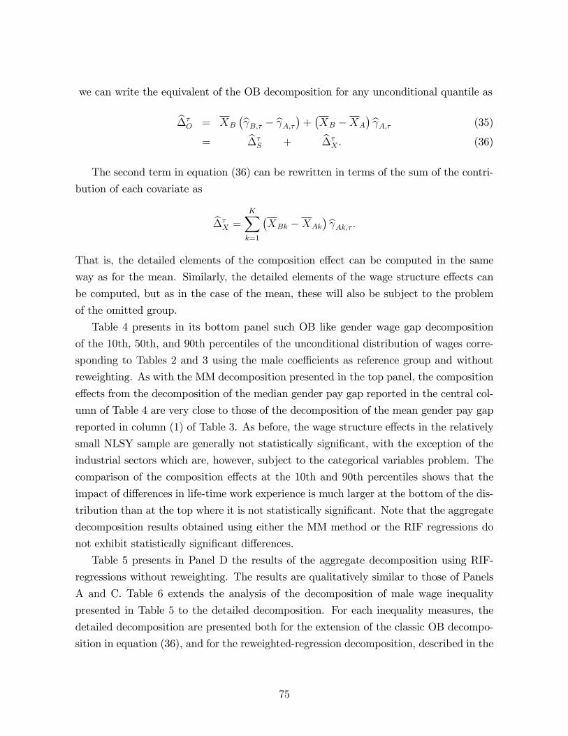
we can write the equivalent of the OB decomposition for any unconditional quantile as

b��O = XB

�b B;� � b A;��+ �XB �XA

� b A;� (35)

= b��S + b��

X : (36)

The second term in equation (36) can be rewritten in terms of the sum of the contri-

bution of each covariate as

b��X =

KXk=1

�XBk �XAk

� b Ak;� :That is, the detailed elements of the composition e¤ect can be computed in the same

way as for the mean. Similarly, the detailed elements of the wage structure e¤ects can

be computed, but as in the case of the mean, these will also be subject to the problem

of the omitted group.

Table 4 presents in its bottom panel such OB like gender wage gap decomposition

of the 10th, 50th, and 90th percentiles of the unconditional distribution of wages corre-

sponding to Tables 2 and 3 using the male coe¢ cients as reference group and without

reweighting. As with the MM decomposition presented in the top panel, the composition

e¤ects from the decomposition of the median gender pay gap reported in the central col-

umn of Table 4 are very close to those of the decomposition of the mean gender pay gap

reported in column (1) of Table 3. As before, the wage structure e¤ects in the relatively

small NLSY sample are generally not statistically signi�cant, with the exception of the

industrial sectors which are, however, subject to the categorical variables problem. The

comparison of the composition e¤ects at the 10th and 90th percentiles shows that the

impact of di¤erences in life-time work experience is much larger at the bottom of the dis-

tribution than at the top where it is not statistically signi�cant. Note that the aggregate

decomposition results obtained using either the MM method or the RIF regressions do

not exhibit statistically signi�cant di¤erences.

Table 5 presents in Panel D the results of the aggregate decomposition using RIF-

regressions without reweighting. The results are qualitatively similar to those of Panels

A and C. Table 6 extends the analysis of the decomposition of male wage inequality

presented in Table 5 to the detailed decomposition. For each inequality measures, the

detailed decomposition are presented both for the extension of the classic OB decompo-

sition in equation (36), and for the reweighted-regression decomposition, described in the

75

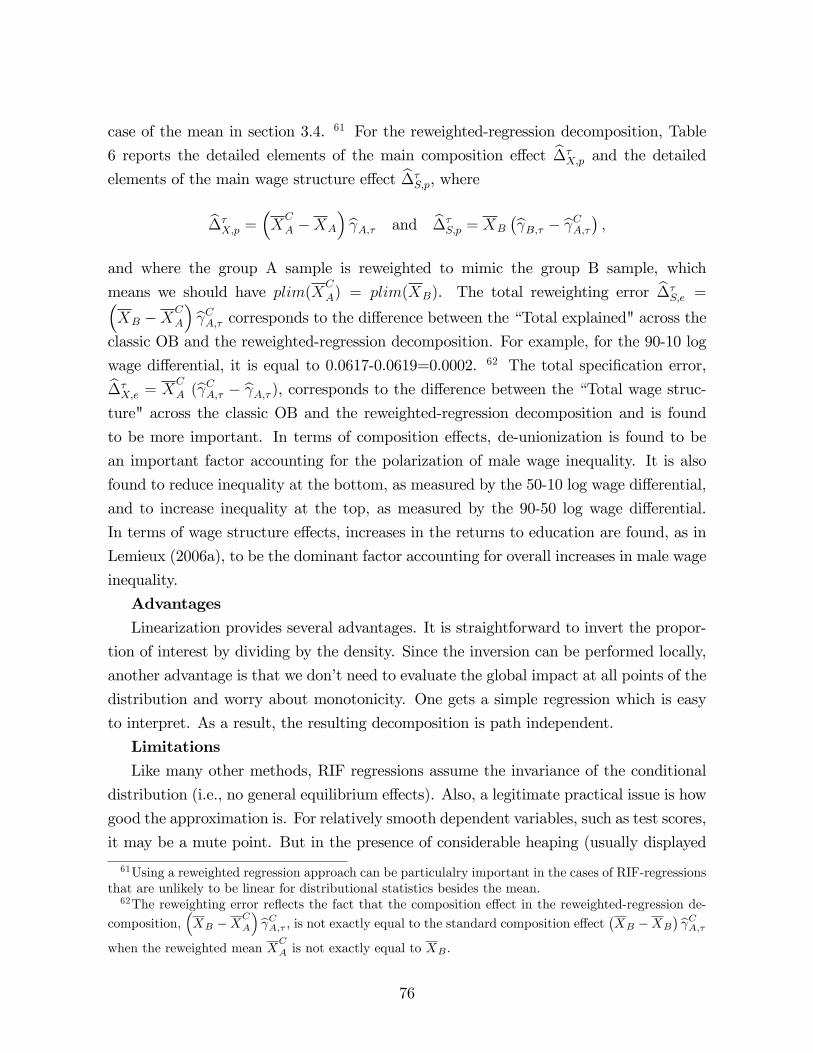
case of the mean in section 3.4. 61 For the reweighted-regression decomposition, Table

6 reports the detailed elements of the main composition e¤ect b��X;p and the detailed

elements of the main wage structure e¤ect b��S;p, where

b��X;p =

�XC

A �XA

�b A;� and b��S;p = XB

�b B;� � b CA;�� ;and where the group A sample is reweighted to mimic the group B sample, which

means we should have plim(XC

A) = plim(XB). The total reweighting error b��S;e =�

XB �XC

A

�b CA;� corresponds to the di¤erence between the �Total explained" across theclassic OB and the reweighted-regression decomposition. For example, for the 90-10 log

wage di¤erential, it is equal to 0.0617-0.0619=0.0002. 62 The total speci�cation error,b��X;e = X

C

A (b CA;� � b A;� ), corresponds to the di¤erence between the �Total wage struc-ture" across the classic OB and the reweighted-regression decomposition and is found

to be more important. In terms of composition e¤ects, de-unionization is found to be

an important factor accounting for the polarization of male wage inequality. It is also

found to reduce inequality at the bottom, as measured by the 50-10 log wage di¤erential,

and to increase inequality at the top, as measured by the 90-50 log wage di¤erential.

In terms of wage structure e¤ects, increases in the returns to education are found, as in

Lemieux (2006a), to be the dominant factor accounting for overall increases in male wage

inequality.

AdvantagesLinearization provides several advantages. It is straightforward to invert the propor-

tion of interest by dividing by the density. Since the inversion can be performed locally,

another advantage is that we don�t need to evaluate the global impact at all points of the

distribution and worry about monotonicity. One gets a simple regression which is easy

to interpret. As a result, the resulting decomposition is path independent.

LimitationsLike many other methods, RIF regressions assume the invariance of the conditional

distribution (i.e., no general equilibrium e¤ects). Also, a legitimate practical issue is how

good the approximation is. For relatively smooth dependent variables, such as test scores,

it may be a mute point. But in the presence of considerable heaping (usually displayed

61Using a reweighted regression approach can be particulalry important in the cases of RIF-regressionsthat are unlikely to be linear for distributional statistics besides the mean.62The reweighting error re�ects the fact that the composition e¤ect in the reweighted-regression de-

composition,�XB �X

C

A

� b CA;� , is not exactly equal to the standard composition e¤ect �XB �XB

� b CA;�when the reweighted mean X

C

A is not exactly equal to XB .

76

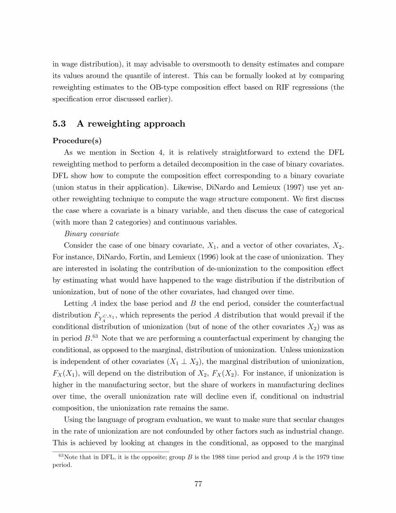
in wage distribution), it may advisable to oversmooth to density estimates and compare

its values around the quantile of interest. This can be formally looked at by comparing

reweighting estimates to the OB-type composition e¤ect based on RIF regressions (the

speci�cation error discussed earlier).

5.3 A reweighting approach

Procedure(s)As we mention in Section 4, it is relatively straightforward to extend the DFL

reweighting method to perform a detailed decomposition in the case of binary covariates.

DFL show how to compute the composition e¤ect corresponding to a binary covariate

(union status in their application). Likewise, DiNardo and Lemieux (1997) use yet an-

other reweighting technique to compute the wage structure component. We �rst discuss

the case where a covariate is a binary variable, and then discuss the case of categorical

(with more than 2 categories) and continuous variables.

Binary covariate

Consider the case of one binary covariate, X1, and a vector of other covariates, X2.

For instance, DiNardo, Fortin, and Lemieux (1996) look at the case of unionization. They

are interested in isolating the contribution of de-unionization to the composition e¤ect

by estimating what would have happened to the wage distribution if the distribution of

unionization, but of none of the other covariates, had changed over time.

Letting A index the base period and B the end period, consider the counterfactual

distribution FYC;X1A

, which represents the period A distribution that would prevail if the

conditional distribution of unionization (but of none of the other covariates X2) was as

in period B.63 Note that we are performing a counterfactual experiment by changing the

conditional, as opposed to the marginal, distribution of unionization. Unless unionization

is independent of other covariates (X1 ? X2), the marginal distribution of unionization,

FX(X1), will depend on the distribution of X2, FX(X2). For instance, if unionization is

higher in the manufacturing sector, but the share of workers in manufacturing declines

over time, the overall unionization rate will decline even if, conditional on industrial

composition, the unionization rate remains the same.

Using the language of program evaluation, we want to make sure that secular changes

in the rate of unionization are not confounded by other factors such as industrial change.

This is achieved by looking at changes in the conditional, as opposed to the marginal

63Note that in DFL, it is the opposite; group B is the 1988 time period and group A is the 1979 timeperiod.

77

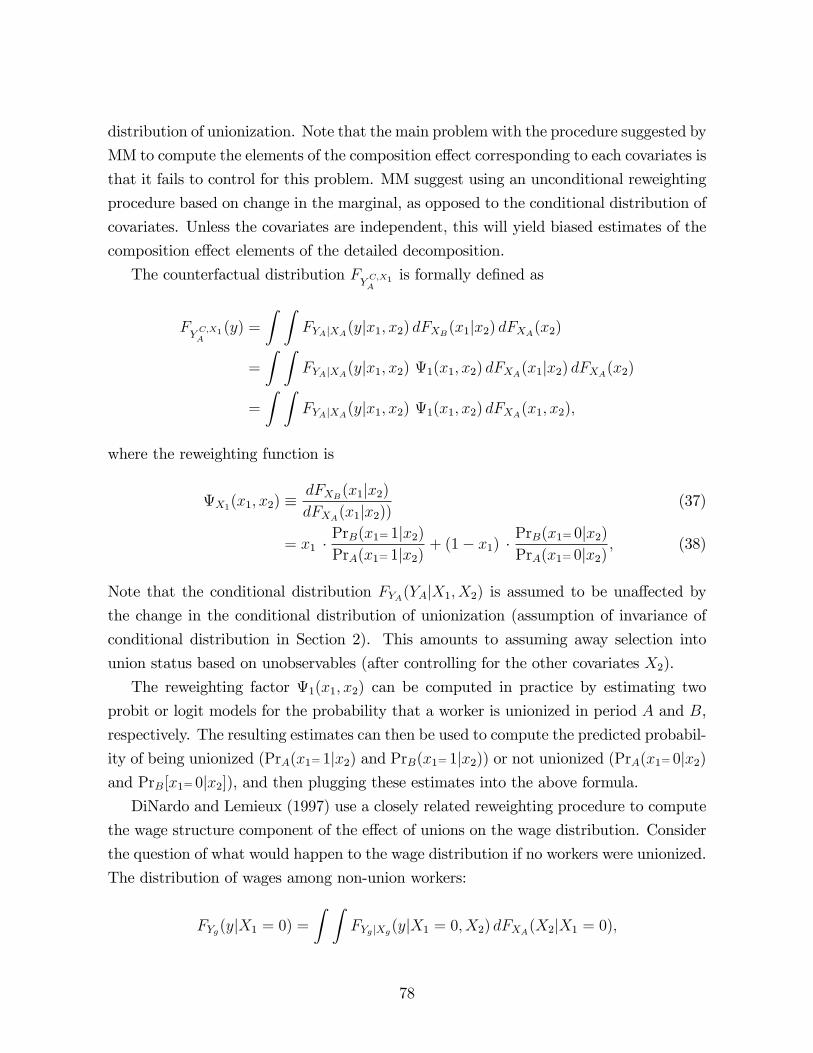
distribution of unionization. Note that the main problem with the procedure suggested by

MM to compute the elements of the composition e¤ect corresponding to each covariates is

that it fails to control for this problem. MM suggest using an unconditional reweighting

procedure based on change in the marginal, as opposed to the conditional distribution of

covariates. Unless the covariates are independent, this will yield biased estimates of the

composition e¤ect elements of the detailed decomposition.

The counterfactual distribution FYC;X1A

is formally de�ned as

FYC;X1A

(y) =

Z ZFYAjXA(yjx1; x2) dFXB(x1jx2) dFXA(x2)

=

Z ZFYAjXA(yjx1; x2) 1(x1; x2) dFXA(x1jx2) dFXA(x2)

=

Z ZFYAjXA(yjx1; x2) 1(x1; x2) dFXA(x1; x2);

where the reweighting function is

X1(x1; x2) �dFXB(x1jx2)dFXA(x1jx2))

(37)

= x1 �PrB(x1= 1jx2)PrA(x1= 1jx2)

+ (1� x1) �PrB(x1= 0jx2)PrA(x1= 0jx2)

; (38)

Note that the conditional distribution FYA(YAjX1; X2) is assumed to be una¤ected bythe change in the conditional distribution of unionization (assumption of invariance of

conditional distribution in Section 2). This amounts to assuming away selection into

union status based on unobservables (after controlling for the other covariates X2).

The reweighting factor 1(x1; x2) can be computed in practice by estimating two

probit or logit models for the probability that a worker is unionized in period A and B,

respectively. The resulting estimates can then be used to compute the predicted probabil-

ity of being unionized (PrA(x1= 1jx2) and PrB(x1= 1jx2)) or not unionized (PrA(x1= 0jx2)and PrB[x1= 0jx2]), and then plugging these estimates into the above formula.DiNardo and Lemieux (1997) use a closely related reweighting procedure to compute

the wage structure component of the e¤ect of unions on the wage distribution. Consider

the question of what would happen to the wage distribution if no workers were unionized.

The distribution of wages among non-union workers:

FYg(yjX1 = 0) =Z Z

FYg jXg(yjX1 = 0; X2) dFXA(X2jX1 = 0);

78

is not a proper counterfactual since the distribution of other covariates, X2, may not be

the same of union and non-union workers. DiNardo and Lemieux (1997) suggest solving

this problem by reweighting non-union workers so that their distribution of X2 is the

same as for the entire workforce. The reweighting factor that accomplishes this at time

A and B are A;S1(X2) and B;S1(X2), respectively, where:

g;S1(X2) =Prg(X1= 0)

Prg(X1= 0jX2); g = A;B:

Using these reweighting terms, we can write the counterfactual distribution of wages

that would have prevailed in absence of unions as:

FYC;S1g

(y) =

Z ZFYg jXg(yjX1 = 0; X2) g;S1(X2) dFXg(X2; X1 = 0); g = A;B:

These various counterfactual distributions can then be used to compute the contri-

bution of unions (or another binary variable x1) to the composition e¤ect, �F (y)X1

, and to

the wage structure e¤ect, �F (y)S1

:

�F (y)X1

= FYA(y)� FY C;X1A(y); (39)

and

�F (y)S1

=hFYA(y)� FY C;S1A

(y)i�hFYB(y)� FY C;S1B

(y)i: (40)

Although we need three di¤erent reweighting factors (X1(x1; x2), A;S1(x2), and

B;S1(x2)) to compute the elements of the detailed wage decomposition corresponding

to x1, these three reweighting factors can be constructed from the estimates of the two

probability models PrA(x1= 1jx2) and PrB(x1= 1jx2). As before, once these reweightingfactors have been computed, the di¤erent counterfactual statistics are easily obtained

using standard statistical packages.

General covariates

It is di¢ cult to generalize the approach suggested above to the case of covariates that

are not binary. In the case of the composition e¤ect, one approach that has been followed

in the applied literature consists of sequentially adding covariates in the probability model

Pr(DB=1jX) used to compute(X).64 For instance, start with Pr(DB=1jX1) , compute1(X1) and the counterfactual statistics of interest by reweighting. Then do the same

64See, for example, Butcher and DiNardo (2002) and Altonji, Bharadwaj, and Lange (2008).

79

thing with Pr(DB=1jX1; X2), etc.One shortcoming of this approach is that the results depend of the order in which the

covariates are sequentially introduced, just like results from a sequential decomposition

for the mean also depend on the order in which the covariates are introduced in the

regression. For instance, estimates the e¤ect of unions that fail to control for any other

covariates may be overstated if union workers tend to be concentrated in industries

that would pay high wages even in the absence of unions. As pointed out by Gelbach

(2009), the problem with sequentially introducing covariates can be thought of as an

omitted variable problem. Unless there are compelling economic reasons for �rst looking

at the e¤ect of some covariates without controlling for the other covariates, sequential

decompositions will have the undesirable property of depending (strongly in some cases)

on the order of the decomposition (path dependence).65

Fortunately, there is a way around the problem of path dependence when performing

detailed decompositions using reweighting methods. The approach however still su¤ers

from the adding-up problem and is more appropriate when only the e¤ect of a particular

factor is of interest. To illustrate this approach, consider a case with three covariates X1,

X2, and X3. In a sequential decomposition, one would �rst control for X1 only, then for

X1 and X2, and �nally for X1, X2, and X3. On the one hand, the regression coe¢ cient on

X1 and/or X2 in regressions that fail to control for X3 are biased because of the omitted

variable problem. The corresponding elements of a detailed OB decomposition for the

mean based on these estimated coe¢ cients would, therefore, be biased too.

On the other hand, the coe¢ cient on the last covariate to be introduced in the re-

gression (X3) is not biased since the other covariates (X1 and X2) are also controlled

for. So although order matters in a sequential regression approach, the e¤ect of the last

covariate to be introduced is not a¤ected by the omitted variable bias.

The same logic applies in the case of detailed decompositions based on a reweight-

ing approach. Intuitively, the di¤erence in the counterfactual distribution one gets by

reweighting with X1 and X2 only, comparing to reweighting with X1, X2, and X3 should

yield the appropriate contribution of X3 to the composition e¤ect.

To see this more formally, consider the group A counterfactual distribution that would

65Both Butcher and DiNardo (2002) and Altonji, Bharadwaj, and Lange (2008) consider cases wherethere is indeed a good reason for following a particular order in the decomposition. For instance, Altonji,Bharadwaj, and Lange (2008) argue that, when looking at various youth outcomes, one should �rstcontrol for predetermined factors like gender and race before controlling for other factors determinedlater in life (AFQT score, educational achievement, etc.). In such a situation, the decomposition iseconometrically interpretable even if gender and race are introduced �rst without controlling for theother factors.

80

prevail if the distribution of X3, conditional on X1, X2, was as in group B:

FYC;X3A

(y) =

ZFYAjXA(yjX)dFXB(X3jX1; X2)dFXA(X1; X2);

=

ZFYAjXA(yjX)X3jX1;X2

(X1; X2)dFXA(X3jX1; X2)dFXA(X1; X2);

=

ZFYAjXA(yjX)X3jX1;X2

(X1; X2)dFXA(X1; X2; X3);

where the reweighting factor X3jX1;X2(X1; X2) can be written as:

X3jX1;X2(X1; X2) �

dFXB(X3jX1; X2)

dFXA(X3jX1; X2)

=dFXB(X1; X2; X3)=dFXB(X1; X2)

dFXA(X1; X2; X3)=dFXA(X1; X2)

= (X1; X2; X3)=X1;X2(X1; X2):

(X1; X2; X3) is the reweighting factor used to compute the aggregate decomposition

in Section 4.5. X1;X2(X1; X1) is a reweighting factor based on all the covariates except

the one considered for the detailed decomposition (X3). As before, Bayes�rule can be

used to show that:

X3jX1;X2(X1; X2) =

Pr(X1; X2jDB = 1)

Pr(X1; X2jDB = 0)=Pr(DB = 1jX1; X2)=Pr(DB = 1)

Pr(DB = 0jX1; X2)=Pr(DB = 0):

Once again, this new reweighting factor is easily computed by running a probit

or logit regression (with X1 and X2 as covariates) and using predicted probability to

estimate X3jX1;X2(X1; X2).

This reweighting procedure for the detailed decomposition is summarized as follows:

1. Compute the reweighting factor using all covariates, (X).

2. For each individual covariate k, compute the reweighting factor using all covariates

but Xk, X�k(X�k).

3. For each covariate k, compute the counterfactual statistic of interest using the ratio

of reweighting factors (X)=X�k(X�k) as weight, and compare it to the counterfactual

statistic obtained using only(X) as weight. The di¤erence is the estimated contribution

of covariate k to the composition e¤ect.

Note that while this procedure does not su¤er from path dependence, the contribution

of each covariates does not sum up to the total contribution of covariates (aggregate

composition e¤ect). The di¤erence is an interaction e¤ect between the di¤erent covariates

81

which is harder to interpret.

AdvantagesThis reweighting procedure shares most of the advantages of the other reweighting

procedures we proposed for the aggregate decomposition. First, it is generally easy to

implement in practice. Second, by using a �exible speci�cation for the logit/probit, it

is possible to get estimates of the various components of the decomposition that de-

pend minimally on functional form assumptions. Third, the procedure yields e¢ cient

estimates.

LimitationsWith a large number of covariates, one needs to compute a sizable number of reweight-

ing factors to compute the various elements of the detailed decomposition. This can be

tedious, although it does not require that much in terms of computations since each

probit/logit is easy to estimate. Another disadvantage of the suggested decomposition

is that although it does not su¤er from the problem of path dependence, we are still left

with an interaction term which is di¢ cult to interpret. For these reasons, we suggest to

�rst use a regression-based approach like the RIF-regression approach discussed above,

which is essentially as easy to compute as a standard OB decomposition. The reweighting

procedure suggested here can then be used to probe these results, and make sure they

are robust to the functional-form assumptions implicit in the RIF-regression approach.

5.4 Detailed decomposition based on conditional quantiles

As we mentioned earlier, the method of Machado andMata (2005) can be used to compute

the wage structure sub-components of the detailed decomposition. These components are

computed by sequentially switching the coe¢ cients of the quantile regressions for each

covariate from their estimated valued for group B to their estimated values for group

A. This sequential switching cannot be used, however, to compute the sub-components

of the composition e¤ect of the detailed decomposition. Rather, Machado and Mata

(2005) suggest an unconditional reweighting approach to do so. This does not provide a

consistent e¤ect since the e¤ect of the reweighted covariate of interest gets confounded by

other covariates correlated with that same covariate. For instance, if union workers are

more concentrated in manufacturing, doing an unconditional reweighting on unions will

also change the fraction of workers in manufacturing. In this sense the e¤ect of unions is

getting confounded by the e¤ect of manufacturing.

This is a signi�cant drawback since it is arguably more important to conduct a detailed

82

decomposition for the composition e¤ect than for the wage structure e¤ect. As discussed

earlier, there are always some interpretation problems with the detailed components of

the wage structure e¤ect because of the omitted group problem.

One solution is to use the conditional reweighting procedure described above instead.

But once this type of reweighting approach is used, there is no need to estimate (condi-

tional) quantile regressions. Unless the quantile regressions are of interest on their own,

it is preferable to use a more consistent approach, such as the one based on the estimation

of RIF-regressions, for estimating the detailed components of both the wage structure

and composition e¤ects.

6 Extensions

In this section, we present three extensions to the decomposition methods discussed

earlier. We �rst consider the case where either the ignorability or the zero conditional

mean assumptions are violated because of self-selection or endogeneity of the covariates.

We next discuss the situation where some of these problems can be addressed when

panel data are available. We conclude the section by discussing the connection between

conventional decomposition methods and structural modelling.

6.1 Dealing with self-selection and endogeneity

The various decomposition procedures discussed up to this point provide consistent es-

timates of the aggregate composition and wage structure e¤ects under the ignorability

assumption. Stronger assumptions, such as conditional mean independence (for decom-

positions of the mean) or straight independence, have to be invoked to perform the

detailed decomposition. In this section we discuss some alternatives for estimating the

decomposition when these assumptions fail. We mostly focus on the case of the OB

decomposition of the mean, though some of the results we present could be extended to

more general distributional statistics.

We consider three scenarios, �rst introduced in Section 2.1.6, under which the OB

decomposition is inconsistent because of a failure of the ignorability or conditional inde-

pendence assumption. In the �rst case, the problem is that individuals from groups A

and B may self-select di¤erently into the labor market. For instance, participation deci-

sions of men (group B) may be di¤erent from participation decisions of women (group

A) in ways that are not captured by observable characteristics. In the second case, we

83

consider what happens when individuals can self-select into group A or B (for instance

union and non-union jobs) on the basis of unobservables. The third case is a standard

endogeneity problem where the covariates are correlated with the error term. For exam-

ple, education (one of the covariate) may be correlated with the error term because more

able individuals tend to get more schooling.

1. Di¤erential self-selection within groups A and B.

One major concern when decomposing di¤erences in wages between two groups with

very di¤erent labor force participation rates is that the probability of participation de-

pends on unobservables " in di¤erent ways for groups A and B. This is a well known

problem in the gender wage gap literature (Blau and Kahn, 2006, Olivetti and Petrongolo,

2008, Mulligan and Rubinstein, 2008, etc.) and in the black-white wage gap literature

(Neal and Johnson, 1996).

Our estimates of decomposition terms may be directly a¤ected when workers of groups

A and B self-select into the labor market di¤erently. Thus, controlling for selection

based on observables and unobservables is necessary to guarantee point identi�cation of

the decomposition terms. If no convincing models for self-selection is available a more

agnostic approach based on bounds has also been recently proposed. Therefore, follow-

ing Machado (2009), we distinguish three branches in the literature of self-selection:i)

selection on observables; ii) selection based on unobservables; iii) bounds.

Selection based on observables and, when panel data are available, on time-invariant

unobserved components can be used to impute values for the missing data on wages of

non-participants. Representative papers of this approach are Neal and Johnson (1996),

Johnson et al. (2000), Neal (2004), Blau and Kahn (2006) and Olivetti and Petrongolo

(2008). These papers are typically concerned with mean or median wages. However,

extensions to cumulative distribution functions or general �-wage gaps could also be

considered.

When labor market participation is based on unobservables, correction procedures

for the mean wages are also available. In these procedures, a control variate is added

as a regressor in the conditional expectation function. The exclusion restriction that an

available instrument Z does not belong to the conditional expectation function also needs

to be imposed.66 Leading parametric and nonparametric examples are Heckman (1974,

1976), Duncan and Leigh (1980), Dolton, Makepeace, and Van Der Klaauw (1989), Vella

66As is well known, selection models can be identi�ed on the basis of functional restrictions even whenan excluded instrumental variable is not available. This is no longer viewed, however, as a credibleidenti�cation strategy. We, therefore, only focus on the case where an instrumental variable is available.

84

(1998), Mulligan and Rubinstein (2008).

In this setting, the decomposition can be performed by adding a control variate

�g(Xi; Zi) to the regression. In most applications, �g(Xi; Zi) is the usual inverse Mills�

ratio term obtain by �tting a probit model of the participation decision. Note that the

addition of this control variate slightly changes the interpretation of the decomposition.

The full decomposition for the mean is now

�� = (�B0 � �A0) +KXk=1

XBk (�Bk � �Ak) + �B(�B � �A)

+

KXk=1

�XBk �XAk

��Ak +

��B � �A

��A:

where �A and �B are the estimated coe¢ cients on the control variates. The decompo-

sition provides a full accounting for the wage gap that also includes di¤erences in both

the composition of unobservables (��B � �A

��A) and in the return to unobservables

(�B(�B � �A)). This treats symmetrically the contribution of observables (the X�s) andunobservables in the decomposition.

A third approach uses bounds for the conditional expectation function of wages for

groups A and B. With those bounds one can come up with bounds for the wage

structure e¤ect, ��S, and the composition e¤ect, �

�X . Let �

�S = E

��E [YBjX;DB = 1]

� E [YAjX;DB = 1]�jDB = 1

�. Then, letting DS be a dummy indicating labor force

participation, we can write the conditional expected wage as,

E [YgjX;Dg] = E [YgjX;Dg; DS = 0]

+Pr (DS = 1jX;Dg) (E [YgjX;Dg; DS = 1]� E [YgjX;Dg; DS = 0])

and therefore

Lg + Pr (DS = 1jX;Dg) (E [YgjX;Dg; DS = 1]� Lg)� E [YgjX;Dg]� Ug + Pr (DS = 1jX;Dg) (E [YgjX;Dg; DS = 1]� Ug)

where Lg and Ug are lower and upper bounds of the distribution of Yg, for g = A;B.

85

Therefore,

(E [YBjX;DB = 1; DS = 1]� E [YAjX;DB = 1; DS = 1]) Pr (DS = 1jX;DB = 1)+ (LB � UA) Pr (DS = 0jX;DB = 1)

� E [YBjX;DB = 1]� E [YAjX;DB = 1]� (E [YBjX;DB = 1; DS = 1]� E [YAjX;DB = 1; DS = 1]) Pr (DS = 1jX;DB = 1)

+ (UB � LA) Pr (DS = 0jX;DB = 1) :

This bounding approach to the selection problem may also use restrictions motivated by

econometric or economic theory to narrow the bounds, as in Manski (1990) and Blundell

et al. (2010).

2. Self-Selection into groups A and B

In the next case we consider, individuals have the choice to belong to either group A

or B. The leading example is the choice of the union status of workers. The traditional

way of dealing with the problem is to model the choice decision and correct for selection

biases using control function methods.67

As discussed in Section 2.1.6, it is also possible to apply instrumental variable methods

more directly without explicitly modelling the selection process into groups A and B.

Angrist and Imbens (1994) show that this will identify the wage gap for the subpopulation

of compliers who are induced by the instrument to switch from one group to the other.

3. Endogeneity of the covariates

The standard assumption used in the OB decomposition is that the outcome variable

Y is linearly related to the covariates, X, and that the error term � is conditionally

independent of X, as in equation (1). Now consider the case where the conditional

independence assumption fails because one or several of the covariates are correlated with

the error term. Note that while the ignorability assumption may hold even if conditional

independence fails, we consider a general case here where neither assumption holds.

As is well known, the conventional solution to the endogeneity problem is to use

instrumental variable methods. For example, if we suspect years of education (one of

the covariate) to be correlated with the error term in the wage equation, we can still

estimate the model consistently provided that we have a valid instrument for years of

67See for instance, the survey of Lewis (1986) who concludes that these methods yield unreliableestimates of the union wage gap. Given these negative results and the lack of credible instrumentsfor unionization, not much progress has been made in this literature over the last two decades. Oneexception is DiNardo and Lee (2004) who use a regression discontinuity design.

86

education. The decomposition can then be performed by replacing the OLS estimates of

the � coe¢ cients by their IV counterparts.

Of course, in most cases it is di¢ cult to come up with credible instrumentation

strategies. It is important to remember, however, that even when the zero conditional

mean assumption E(�jX) = 0 fails, the aggregate decomposition may remain valid,

provided that ignorability holds. This would be the case, for example, when unobserved

ability is correlated with education, but the correlation (more generally the conditional

distribution of ability given education) is the same in group A and B. While we are not

able to identify the contribution of education vs. ability in this context (unless we have

an instrument), we know that they are no systematic ability di¤erences between groups

A and B once we have controlled for education. As a result, the aggregate decomposition

remains valid.

6.2 Panel data

An arguably better way of dealing with the selection and endogeneity problems mentioned

above is to use panel data. Generally speaking, panel data methods can be used to

compute consistent estimates of the ��s in each of the three cases discussed earlier. For

example, if the zero conditional mean assumption holds once we also control for a person-

speci�c �xed e¤ects �i in a panel of length T (E(�itjXi1; ::; XiT ; �i)), we can consistently

estimate � using standard panel data methods (�xed e¤ects, �rst di¤erences, etc.). This

provides an alternative way of dealing with endogeneity problems when no instrumental

variables are available.

As we also discussed earlier, panel data can be used to impute wages for years where

an individual is not participating in the labor market (e.g. Olivetti and Petrongolo

(2008)). Note that in cases where groups are mutually exclusive (e.g. men vs. women),

it may still be possible to estimate �xed e¤ect models if the basic unit used is the �rm (or

related concepts) instead, or in addition to the individual (Woodstock, 2008). Care has

to be exercised in those circumstances to ensure that the �rm �xed e¤ect is the same for

both female and male employees of the same �rm. Another important issue with these

models is the di¢ culty of interpretation of the di¤erences in male and female intercepts

which may capture the unobserved or omitted individual and �rm e¤ects.

Panel data methods have also been used to adjust for the selection into groups in cases

where the same individual is observed in group A and B. For example, Freeman (1984)

and Card (1996) estimate the union wage gap with panel data to control for the selection

87

of workers into union status. Lemieux (1998) uses a more general approach where the

return to the �xed e¤ect may be di¤erent in the union and non-union sector. He also

shows how to generalize the approach to the case of a decomposition of the variance.

Without loss of generality, assume that the return to the �xed e¤ect for non-union

workers (group A) is 1, while it is equal to �B for union workers. The mean decomposition

adjusted for �xed e¤ects yields:

�� = (�B0 � �A0) +KXk=1

XBk (�Bk � �Ak) + �B(�B � 1)

+

KXk=1

�XBk �XAk

��Ak +

��B � �A

�:

The interpretation of the decomposition is the same as in a standard OB setting

except that��B � �A

�now represents the composition e¤ect term linked to non-random

selection into the union sector, while the wage structure term �B(�B � 1) captures acorresponding wage structure e¤ect.

More sophisticated model with several levels of �xed e¤ects have also been used in

practice. For instance, Abowd et al. (2008) decompose inter-industry wage di¤erentials

into various components that include both individual- and �rm-speci�c �xed e¤ects.

6.3 Decomposition in structural models

In Section 2, we pointed out that decomposition methods were closely related to meth-

ods used in the program evaluation literature where it is not necessary to estimate a

fully speci�ed structural model to estimate the main parameter of interest (the ATT ).

Provided that the ignorability assumption is satis�ed, we can perform an aggregate de-

composition without estimating an underlying structural model.

There are some limits, however, to what can achieved without specifying any structure

to the underlying economic problem. As we just discussed in Section 6.1, one problem

is that the ignorability assumption may not hold. Under this scenario, more explicit

modelling may be useful for correcting biases in the decomposition due to endogeneity,

self-selection, etc.

Another problem that we now address concerns the interpretation of the wage struc-

ture components of the detailed decomposition. Throughout this chapter, we have pro-

posed a number of ways of estimating these components for both the mean and more

general distributional statistics. In the case of the mean, the interpretation of the de-

88

tailed decomposition for the wage structure e¤ect is relatively straightforward. Under

the assumption (implicit in the OB decomposition) that the wage equations are truly

linear and the errors have a zero conditional mean, we can think of the wage setting

model as a fully specify structural model. The � coe¢ cients are the �deep�structural

parameters of the model, and these structural parameters are used directly to perform

the decomposition.

Things become more complicated once we go beyond the mean. For instance, in the

case of the variance (section 4.1), recall that the wage structure e¤ect from equation (26)

which depends on the parameters of both the models for the conditional mean (�) and

for the variance (�).

Take, for example, the case where one of the covariates is the union status of workers.

The parameter � captures the �compression�, or within-group, e¤ect, while the para-

meter � captures the �wage gap�, or between-group, e¤ect. These two terms have a

distinct economic interpretation as they re�ect di¤erent channels through which union

wage policies tend to impact the wage distribution.

In the case of more general distributional statistics, the wage structure e¤ect depends

on an even larger number of underlying parameters capturing the relationship between the

covariates and higher order moments of the distribution. As a result, the wage structure

part of the detailed decomposition becomes even harder to interpret, as it potentially

depends on a large number of underlying parameters.

In some cases, this may not pose a problem from an interpretation point of view. For

instance, we may only care about the overall e¤ect of unions, irrespective of whether it is

coming from a between- or within-group e¤ect (or corresponding components for higher

order moments). But in other cases this type of interpretation may be unsatisfactory.

Consider, for example, the e¤ect of education on the wage structure. Like unions, edu-

cation may in�uence wage dispersion through a between- or within-group channel. The

between-group component is linked to the traditional return to education (e¤ect on con-

ditional means), but education also has a substantial e¤ect on within-group dispersion

(see, e.g., Lemieux, 2006b). All these e¤ects are combined together in the decomposition

methods proposed in Section 5, which is problematic if we want to know, for instance,

the speci�c contribution of changes in the return to education to the growth in wage

inequality.

In these circumstances, we need to use a more structural approach to get a more

economically interpretable decomposition of the wage structure e¤ect. The decomposi-

tion method of Juhn, Murphy and Pierce (1993) is, in fact, an early example of a more

89

structurally-based decomposition. In their setting, the model for the conditional mean

is interpreted as an underlying human capital pricing equation. Likewise, changes in

residual wage dispersion (given X) are interpreted as re�ecting an increase in the return

to unobservable skills.

As we discussed in Section 4.3, the fact that Juhn, Murphy and Pierce (1993)�s

provides a richer interpretation of the wage structure e¤ect by separating the within- and

between-group components is an important advantage of the method. We also mentioned,

however, that the interpretation of the decomposition was not that clear for distributional

statistics going beyond the variance, and that the procedure typically imposes substantial

restrictions on the data that may or may not hold. By contrast, a method like DFL

imposes very little restrictions (provided that the probit/logit model used for reweighting

is reasonably �exible), though it is more limited in terms of the economic interpretation

of the wage structure e¤ect.

In light of this, the challenge is to �nd a way of imposing more explicit structure on the

economic problemwhile making sure the underlying model ��ts�the data reasonably well.

One possible way of achieving this goal is to go back to the structural form introduced in

Section 2 (Ygi = mg (Xi; "i)), and use recent results from the literature on nonparametric

identi�cation of structural functions to identify the functions mg(�). As discussed inSection 2.2.1, this can be done by invoking results obtained by Matzkin (2003), Blundell

and Powell (2007) and Imbens and Newey (2009). Generally speaking, it is possible to

identify the functions mg(�) nonparametrically under the assumptions of independenceof " (Assumption 8), and strict monotonicity of mg(�) in " (Assumption 9).But while it is possible, in principle, to nonparametrically identify the functionsmg(�),

there is no guarantee that the resulting estimates will be economically interpretable. As

a result, a more common approach used in the empirical literature is to write down a

more explicit (and parametric) structural model, but carefully look at whether the model

adequately �ts the data. Once the model has been estimated, simulation methods can

then be used to compute a variety of counterfactual exercises. The counterfactuals then

form the basis of a more economically interpretable decomposition of the wage structure

e¤ect.

To take a speci�c example, consider Keane and Wolpin (1997) model of career pro-

gression of young men where educational and occupational choices are explicitly modeled

using a dynamic programming approach. After carefully looking at whether the estimated

model is rich enough to adequately �t the distribution of wages, occupational choices,

and educational achievement, Keane and Wolpin use the estimated model to decompose

90

the distribution of lifetime utility (itself computed using the model). They conclude

that 90 percent of the variance of lifetime utility is due to skill endowment heterogeneity

(schooling at age 16 and unobserved type). By contrast, choices and other developments

happening after age 16 have a relatively modest impact on the variance of lifetime util-

ity.68 The general idea here is to combine structural estimation and simulation methods

to quantify the contribution of the di¤erent parameters of interest to some decomposi-

tions of interest. These issues are discussed in more detail in the chapter on structural

methods by Keane, Wolpin, and Todd (2010).

One last point is that the interpretation problem linked to the wage structure e¤ect

does not apply to the detailed decomposition for the composition e¤ect. In that case,

each component is based on a clear counterfactual exercise that does not require an

underlying structure to be interpretable. The aggregate decomposition is based on the

following counterfactual exercise: what would be the distribution of outcomes for group A

if the distribution of the covariates for group A were the same as for group B? Similarly,

the detailed decomposition is based on a conditional version of the counterfactual. For

example, one may want to ask what would be the distribution of outcomes for group A

if the distribution of unionization (or another covariate) for group A was the same as for

group B, conditional on the distribution of the other covariates remaining the same.

These interpretation issues aside, it may still be useful to use a more structural

approach when we are concerned about the validity of the decomposition because of

self-selection, endogeneity, etc. For instance, in Keane and Wolpin (1997), the choice of

schooling and occupation is endogenous. Using standard decomposition methods to look,

for instance, at the contribution of the changing distribution of occupations to changes

in the distribution wages would yield invalid results because occupational choice is en-

dogenous. In such a context, structural modelling, like the IV and selection methods

discussed in Section 6.1, can help recover the elements of the decomposition when stan-

dard methods fail because of endogeneity or self-selection. But the problem here is quite

distinct from issues with the wage structure e¤ect where standard decomposition meth-

ods are limited because of an interpretation problem, and where structural modelling

provides a natural way of resolving this interpretation problem. By contrast, solutions

to the problem of endogeneity or self-selection are only as a good as the instruments (or

related assumptions) used to correct for these problems. As a result, the value added of

68Note, however, that Ho¤man (2009) �nds that skill endowments have a sizably smaller impactin a richer model that incorporates comparative advantage (across occupations), search frictions, andexogenous job displacement.

91

the structural approach is much more limited in the case of the composition e¤ect than

in the case of the wage structure e¤ect.

This last point is very clear in the emerging literature where structural modelling is

used in conjunction with experimental data. For example, Card and Hyslop (2005) use

experimental data from the Self Su¢ ciency Project (SSP) to look at why individuals

o¤ered with a generous work subsidy are less likely to receive social assistance (SA).

By de�nition, there is no composition e¤ect since the treatment and control groups are

selected by random assignment. In that context, the average treatment e¤ect precisely

corresponds to the wage structure e¤ect (or �SA� structure e¤ect in this context) in

a decomposition of the di¤erence between the treatment and control group. It is still

useful, however, to go beyond this aggregate decomposition to better understand the

mechanisms behind the measured treatment e¤ect. Card and Hyslop (2005) do so by

estimating a dynamic search model.

This provides much more insight into the �black box�of the treatment e¤ect than

what a traditional decomposition exercise would yield. Remember that the detailed wage

structure component in a OB type decomposition is based on the di¤erence between the

return to di¤erent characteristics in the two groups. In a pure experimental context like

the SSP project, this simply re�ects some heterogeneity in the treatment e¤ect across

di¤erent subgroups. Knowing about the importance of heterogeneity in the treatment

e¤ect is important from the point of view of the generalizability of the results. But unlike

a structural approach, it provides relatively little insight on the mechanisms underlying

the treatment e¤ect.

7 Conclusion

The development of new decomposition methods has been a fertile area of research over

the last 10-15 years. Building on the seminal work of Oaxaca (1973) and Blinder (1973), a

number of procedures that go beyond the mean have been suggested and used extensively

in practice. In this chapter, we have reviewed these methods and suggested a number of

�best practices�for researchers interested in these issues. We have also illustrated how

these methods work in practice by discussing existing applications and working through

a set of empirical examples throughout the chapter.

Another important and recent development in this literature has linked decomposition

methods to the large and growing literature on program evaluation and treatment e¤ects.

This connection is useful for several reasons. First, it helps clarify some interpretation

92

issues with decompositions. In particular, results from the treatment e¤ect literature can

be used to show, for example, that we can give a structural interpretation to an aggregate

decomposition under the assumption of ignorability. Another bene�t of this connection

is that formal results about the statistical properties of treatment e¤ect estimators can

also be directly applied to decomposition methods. This helps guide the choice of decom-

position methods that have good statistical properties, and conduct inference on these

various components of the estimated decomposition.

But this connection with the treatment e¤ect literature also comes at a cost. While

no structural modelling is required to perform a decomposition or estimate a treatment

e¤ect, these approaches leave open the question of what are the economic mechanisms

behind the various elements of the decomposition (or behind the treatment e¤ect). Now

that the connection between decomposition methods and the treatment e¤ect literature

has been well established, an important direction for future research will be to improve

the connection between decomposition methods and structural modelling.

The literature on inequality provides some useful hints on how this connection can

be useful and improved upon. In this literature, decomposition methods have helped

uncover the most important factors behind the large secular increase in the distribution

of wages. Those include the return to education, de-unionization, and the decline in

the minimum wage, to include a few examples. These �ndings have spurred a large

number of more conceptual studies trying to provide formal economic explanations for

these important phenomena. In principle, these explanations can then be more formally

confronted to the data by writing down and estimating a structural model, and using

simulation methods to quantify the role of these explanations.

This suggest a two-step research strategy where �over the shelf�decomposition meth-

ods, like those discussed in this chapter, can �rst be used to uncover the main forces un-

derlying an economic phenomenon of interest. More �structural�decomposition methods

could then be used to better understand the economics behind the more standard de-

composition results. We expect such a research strategy to be a fruitful area of research

in the years to come.

References

Abowd, John M., Francis Kramarz, Paul Lengerman, and Sebastien Roux (2008), �Per-

sistent Inter-Industry Wage Di¤erences: Rent Sharing and Opportunity Costs"

Working paper.

93

Albrecht, James, Anders Björklund, and Susan Vroman (2003), �Is There a Glass

Ceiling in Sweden?" Journal of Labor Economics 21: 145-178.

Altonji, Joseph G. and Rebecca Blank (1999), �Race and Gender in the Labor Market,"

in Handbook of Labor Economics, Vol. 3C, ed. by O. Ashenfelter, and D. Card.

Elsevier Science, Amsterdam.

Altonji, Joseph G. and Rosa L. Matzkin (2005), �Cross Section and Panel Data Esti-

mators for Nonseparable Models with Endogenous Regressors," Econometrica, 73:

1053-1102.

Altonji, Joseph G., P. Bharadwaj, and Fabian Lange (2008), �Changes in the charac-

teristics of American youth: Implications for adult outcomes. Working paper, Yale

University.

Angrist, Joshua and Guido W. Imbens (1994), �Identi�cation and Estimation of Local

Average Treatment E¤ects�, Econometrica 62: 467�476.

Athey, Susan and Guido W. Imbens (2006), �Identi�cation and Inference in Nonlinear

Di¤erence-In-Di¤erencesModels," Econometrica 74: 431-497.

Autor, David H., Frank Levy, and Richard Murnane (2003), �The Skill Content of

Recent Technological Change: An Empirical Exploration," Quarterly Journal of

Economics 118: 1279-1333.

Autor, David H., Lawrence B. Katz and Melissa S. Kearney (2005), �Rising Wage

Inequality: The Role of Composition and Prices.�NBERWorking Paper No. 11628,

September.

Barsky, R., John Bound, K. Charles, and J. Lupton (2002), �Accounting for the Black-

White Wealth Gap: A Nonparametric Approach,�Journal of the American Statis-

tical Association 97: 663-673.

Bauer, Thomas K., Silja Göhlmann, and Mathias Sinning (2007), �Gender di¤erences

in smoking behavior", Health Economics 19: 895�909.

Bauer, Thomas K. and Mathias Sinning (2008), �An Extension of the Blinder�Oaxaca

Decomposition to Nonlinear Models", Advances in Statistical Analysis 92: 197�206.

Bertrand, Marianne, and Kevin F. Hallock (2001), �The Gender Gap in Top Corporate

Jobs," Industrial and Labor Relations Review 55: 3-21.

94

Biewen, Martin (2001), �Measuring the E¤ects of Socio-Economic Variables on the

Income Distribution: An Application to the Income Distribution: An Application

to the East German Transition Process�, Review of Economics and Statistics 83:

185-190.

Bitler, Marianne P., Jonah B. Gelbach, and Hilary W. Hoynes (2006), �What Mean

Impacts Miss: Distributional E¤ects of Welfare Reform Experiments� American

Economic Review 96: 988-1012.

Black, Dan, Amelia Haviland, Seth Sanders, and Lowell Taylor (2008), �Gender Wage

Disparities among the Highly Educated", Journal of Human Resources 43: 630-659.

Blau, Francine D. and Lawrence M. Kahn (1992), �The Gender Earnings Gap: Learning

from International Comparisons", American Economic Review 82: 533�538.

Blau, Francine D. and Lawrence M. Kahn (1997), �Swimming Upstream: Trends in the

Gender Wage Di¤erential in the 1980s," Journal of Labor Economics 15: 1-42.

Blau, Francine D. and Lawrence M. Kahn (2003), �Understanding International Di¤er-

ences in the Gender Pay Gap," Journal of Labor Economics 21: 106�144.

Blau, Francine D. and Lawrence M. Kahn (2006), �The US gender pay gap in the 1990s:

Slowing convergence," Industrial & Labor Relations Review, 60(1): 45-66.

Blinder, Alan (1973), �Wage Discrimination: Reduced Form and Structural Estimates,�

Journal of Human Resources 8:436�455.

Blundell, Richard, and James L. Powell (2007), �Censored regression quantiles with

endogenous regressors," Journal of Econometrics 141: 65-83.

Blundell, Richard, Martin Browning , and Ian Crawford (2010), �Best Nonparametric

Bounds on Demand Responses," Econometrica 76: 1227�1262.

Bourguignon, Francois (1979), �Decomposable Income Inequality Measures", Econo-

metrica 47: 901�920

Bourguignon, F. and Francisco H.G. Ferreira (2005), �Decomposing Changes in the

Distribution of Household Incomes: Methodological Aspects," in The Microeco-

nomics of Income Distribution Dynamics in East Asia and Latin America," F.

Bourguignon, F.H.G. Ferreira and N. Lustig (eds.) World Bank. pp. 17-46.

95

Bourguignon,F. , Francisco H.G. Ferreira, and Philippe G. Leite (2008), "Beyond Oaxaca�

Blinder: Accounting for di¤erences in household income distributions," Journal of

Economic Inequality 6: 117-148.

Busso, Matias, John DiNardo, and Justin McCrary (2009), �New Evidence on the Finite

Sample Properties of Propensity Score Matching and Reweighting Estimators�IZA

Discussion Paper No. 3998.

Butcher, Kristin F. and John DiNardo (2002), "The Immigrant and native-born wage

distributions: Evidence from United States censuses," Industrial and Labor Rela-

tions Review 56: 97-121.

Cain, Glen (1986), �The Economic Analysis of Labor Market Discrimination: a Survey,�

in Ashenfelter, O.C. and R. Layard, editors, Handbook of Labor Economics, North-

Holland, vol 1, pp.709-730

Card, David (1992), �The E¤ects of Unions on the Distribution of Wages: Redistribution

or Relabelling?�NBER Working Paper 4195, Cambridge: Mass.: National Bureau

of Economic Research, 1992.

Card, David (1996), �The E¤ect of Unions on the Structure of Wages: A Longitudinal

Analysis�, Econometrica 64: 957-979.

Card, David, and Dean R. Hyslop (2005), �Estimating the E¤ects of a Time-Limited

Earnings Subsidy for Welfare-Leavers�, Econometrica 73:1723�1770.

Chay, Kenneth Y., and David S. Lee (2000), �Changes in Relative Wages in the 1980s:

Returns to Observed and Unobserved Skills and Black-White Wage Di¤erentials,�

Journal of Econometrics, 99(1), 1-38.

Chernozhukov, Victor, Ivan Fernandez-Val, and Blaise Melly (2009), �Inference on

Counterfactual Distributions," forthcoming in Econometrica.

Chernozhukov, Victor, Ivan Fernandez-Val, and A. Galichon (2010), �Quantile and

Probability Curves without Crossing," forthcoming in Econometrica.

Chiquiar, Daniel and Gordon H. Hanson (2005), �International migration, self-selection,

and the distribution of wages: Evidence from Mexico and the United States",

Journal of Political Economy 113: 239-281.

96

Cowell, Frank A. (1980), �On the Structure of Additive Inequality Measures", Review

of Economic Studies 47: 521�531.

Denison, E.F. (1962), The sources of economic growth in the United States and the

alternatives before us, Supplementary Paper No. 13, New York, Committee for

Economic Development.

DiNardo, John, Nicole M. Fortin, and Thomas Lemieux (1996), �Labor Market Insti-

tutions and the Distribution of Wages, 1973-1992: A Semiparametric Approach,�

Econometrica 64: 1001-1044.

DiNardo, John, and David S. Lee (2004), �Economic Impacts of New Unionization On

Private Sector Employers: 1984-2001,�The Quarterly Journal of Economics 119:

1383-1441.

DiNardo, John and Thomas Lemieux (1997), �Diverging Male Inequality in the United

States and Canada, 1981-1988: Do Institutions Explain the Di¤erence,�Industrial

and Labor Relations Review 50: 629-651.

Dolton, Peter John, Gerald Henry Makepeace and Wilbert Van Der Klaauw (1986),

�Sample Selection and Male-Female Earnings Di¤erentials in the Graduate Labour

Market". Oxford Economic Papers 38: 317�341.

Doiron, Denise J. and W. Craig Riddell (1994) �The Impact of Unionization on Male-

Female Earnings Di¤erences in Canada," Journal of Human Resources 29: 504-534.

Donald, Stephen G., David A. Green, and Harry J. Paarsch (2000), �Di¤erences in

Wage Distributions between Canada and the United States: An Application of a

Flexible Estimator of Distribution Functions in the Presence of Covariates Source�

Review of Economic Studies 67: 609-633.

Duncan, Gregory M. and Duane E. Leigh (1980), �Wage Determination in the Union and

Nonunion Sectors: A Sample Selectivity Approach,�Industrial and Labor Relations

Review 34: 24-34

Egel, Daniel, Bryan Graham, and Cristine Pinto (2009), �E¢ cicient Estimation of Data

Combination Problems by the Method of Auxiliary-to-Study Tilting." Mimeo.

Even, William E. and David A. Macpherson (1990), Plant size and the decline of union-

ism", Economics Letters 32: 393�398

97

Fairlie, Robert W. (1999), The absence of the african-american owned business: an

analysis of the dynamics of self�employment", Journal of Labor Economics 17:

80�108.

Fairlie, Robert W. (2005), �An Extension of the Blinder-Oaxaca Decomposition Tech-

nique to Logit and Probit Models", Journal of Economic and Social Measurement

30: 305�316.

Fields, Judith, and Edward N.Wol¤ (1995), �Interindustry Wage Di¤erentials and the

Gender Wage Gap." Industrial and Labor Relations Review 49: 105-120.

Firpo, Sergio (2007), �E¢ cient Semiparametric Estimation of Quantile Treatment Ef-

fects,�Econometrica, 75: 259 - 276.

Firpo, Sergio (2010), �Identi�cation and Estimation of Distributional Impacts of Inter-

ventions Using Changes in Inequality Measures�EESP-FGV, mimeo.

Firpo, Sergio, Nicole M. Fortin, and Thomas Lemieux (2007), �Decomposing Wage Dis-

tributions using Recentered In�uence Functions Regressions", mimeo, University

of British Columbia.

Firpo, Sergio, Nicole M. Fortin, and Thomas Lemieux (2009) �Unconditional Quantile

Regressions,�Econometrica 77(3): 953-973.

Fitzenberger, Bernd, Karsten Kohn and Qingwei Wang (2009), �The Erosion of Union

Membership in Germany: Determinants, Densities, Decompositions", Journal of

Population Economics, forthcoming.

Foresi, Silverio and Franco Peracchi (1995), �The Conditional Distribution of Excess

Returns: an Empirical Analysis", Journal of the American Statistical Association

90: 451-466.

Fortin, Nicole M., and Thomas Lemieux (1998), �Rank Regressions, Wage Distributions,

and the Gender Gap", Journal of Human Resources 33: 610�643.

Fortin, Nicole M. (2008), �The Gender Wage Gap among Young Adults in the United

States: The Importance of Money vs. People,�Journal of Human Resources, 43:

886-920.

Freeman, Richard B. (1980), �Unionism and the Dispersion of Wages,�Industrial and

Labor Relations Review 34: 3-23.

98

Freeman, Richard B. (1984), �Longitudinal Analysis of the E¤ect of Trade Unions,"

Journal of Labor Economics 2: 1-26.

Freeman, Richard B. (1993), �How Much has Deunionization Contributed to the Rise of

Male Earnings Inequality?�In Sheldon Danziger and Peter Gottschalk, eds. Uneven

Tides: Rising Income Inequality in America. New York: Russell Sage Foundation,

133-63.

Frolich, Markus (2004), �Finite-Sample Properties of Propensity-Score Matching and

Weighting Estimators,�Review of Economics and Statistics 86: 77-90.

Gardeazabal, Javier and Arantza Ugidos (2004), �More on the Identi�cation in Detailed

Wage Decompositions,�Review of Economics and Statistics 86: 1034�57.

Gelbach, Jonah B. (2002), �Identi�ed Heterogeneity in Detailed Wage Decompositions,"

mimeo, University of Maryland at College Park.

Gelbach, Jonah B. (2009), �When Do Covariates Matter? And Which Ones, and How

Much?" mimeo, Eller College of Management, University of Arizona.

Gomulka, Joanna and Nicholas Stern (1990), �The employment of married women in

the United Kingdom, 1970�1983", Economica 57: 171�199.

Gosling, Amanda, Stephen Machin, and Costas Meghir (2000), "The Changing Distri-

bution of Male Wages in the U.K," Review of Economic Studies 67: 635-666.

Greene, William H. (2003), Econometric Analysis. 5th ed. Upper Saddle River, NJ:

Pearson Education

Heckman, James (1974), �Shadow Prices, Market Wages and Labor Supply," Econo-

metrica 42: 679�694.

Heckman, James (1976), �The Common Structure of Statistical Models of Truncation,

Sample Selection and Limited Dependent Variables and a Simple Estimator for

Such Models,�Annals of Economic and Social Measurement 5: 475-492.

Heckman, James (1979), �Sample Selection Bias as a Speci�cation Error,�Econometrica

47: 153-163.

99

Heckman, James J., Je¤rey Smith and Nancy Clements (1997), �Making the Most Out

of Programme Evaluations and Social Experiments: Accounting for Heterogeneity

in Programme Impacts", Review of Economic Studies, 64(4): 487�535.

Heckman, James J., Hidehiko Ichimura, and Petra Todd (1997), �Matching As An

Econometric Evaluation Estimator: Evidence from Evaluating a Job Training Pro-

gramme," Review of Economic Studies, 64: 605-654.

Heckman, James J., Hidehiko Ichimura, Je¤rey Smith and Petra Todd (1998), �Char-

acterizing Selection Bias Using Experimental Data," Econometrica 66: 1017-1098.

Heywood, John S. and Daniel Parent (2008), �The White-Black Wage Gap and the

Method of Pay," mimeo, McGill University.

Hirano, Kiesuke, Guido W. Imbens, and Geert Ridder, (2003), �E¢ cient Estimation of

Average Treatment E¤ects Using the Estimated Propensity Score,�Econometrica

71, 1161�1189.

Holland, Paul W. (1986), �Statistics and Causal Inference," Journal of the American

Statistical Association 81(396): 945-960.

Ho¤man, Florian (2009), �An Empirical Model of Life-Cycle Earnings and Mobility

Dynamics,�University of Toronto, Department of Economics, mimeo.

Horrace, William and Ronald L. Oaxaca (2001), �Inter-Industry Wage Di¤erentials and

the Gender Wage Gap: An Identi�cation Problem," Industrial and Labor Relations

Review, 54: 611-618.

Imbens, Guido W. and Whitney K. Newey (2009) �Identi�cation and Estimation of Tri-

angular Simultaneous Equations Models Without Additivity," Econometrica 77(5):

1481 - 1512.

Jann, Ben (2005), �Standard Errors for the Blinder-Oaxaca Decomposition", German

Stata Users�GroupMeetings 2005. Available from http://repec.org/dsug2005/oaxaca

se handout.pdf.

Jann, Ben (2008), �The Oaxaca-Blinder Decomposition for Linear Regression Models,"

Stata Journal 8: 435�479.

Jones, Frank Lancaster (1983), �On Decomposing the Wage Gap: A Critical Comment

on Blinder�s Method", Journal of Human Resources 18: 126�130.

100

Johnson, William, Yuichi Kitamura, and Derek Neal (2000), �Evaluating a Simple

Method for Estimating Black-White Gaps in Median Wages," American Economic

Review 90:339�343.

Jorgenson, D. W. and Z. Griliches (1967), �The Explanation of Productivity Change�

Review of Economic Studies 34: 249-283

Juhn, Chinhui, Kevin M. Murphy, and Brooks Pierce (1991), �Accounting for the Slow-

down in Black-White Wage Convergence," in Workers and Their Wages: Changing

Patterns in the United States, ed. by M. H. Kosters. American Enterprise Institute,

Washington.

Juhn, Chinhui, Kevin M. Murphy, and Brooks Pierce (1993), �Wage Inequality and the

Rise in Returns to Skill,�Journal of Political Economy 101: 410-442.

Keane, Michael P. and Kenneth I. Wolpin (1997), �The Career Decisions of Young

Men,�Journal of Political Economy, 105: 473-522.

Keane, Michael P., Kenneth I. Wolpin, and Petra Todd (2010), �Dynamic Structure

Modeling," in Handbook of Labor Economics, Vol. 4, ed. by O. Ashenfelter, and

D. Card. Elsevier Science, Amsterdam.

Kendrick, John W. (1961), Productivity Trends in the United States, Princeton, Prince-

ton University Press.

Kennedy, Peter (1986), �Interpreting Dummy Variables," Review of Economics and

Statistics 68): 174-175.

Kline, Pat (2009), �Blinder-Oaxaca as a Reweighting Estimator�UC Berkeley mimeo.

Koenker, Roger and G. Bassett (1978), �Regression Quantiles,�Econometrica, 46, 33-

50.

Krueger, Alan B. and Lawrence H. Summers (1988), �E¢ ciency Wages and the Inter-

Industry Wage Structure," Econometrica 56(2): 259-293.

Krieg, John M. and Paul Storer (2006), �How Much Do Students Matter? Applying

the Oaxaca Decomposition to Explain Determinants of Adequate Yearly Progress,"

Contemporary Economic Policy, 24: 563�581.

101

Leibbrandt, Murray, James A. Levinsohn, and Justin McCrary (2005), �Incomes in

South Africa Since the Fall of Apartheid�NBER Working Paper 11384

Lemieux, Thomas (2002), �Decomposing Changes in Wage Distributions: a Uni�ed

Approach,�The Canadian Journal of Economics 35: 646-688.

Lemieux, Thomas (2006a), �Post-secondary Education and Increasing Wage Inequal-

ity", American Economic Review 96: 195-199.

Lemieux, Thomas (2006b),�Increasing Residual Wage Inequality: Composition E¤ects,

Noisy Data, or Rising Demand for Skill?", American Economic Review 96: 461-498.

Lewis, H. Gregg (1963), Unionism and Relative Wages in the United States, Chicago:

University of Chicago Press.

Lewis, H. Gregg (1986), Union Relative Wage E¤ects: A Survey, Chicago: University

of Chicago Press.

Neumark, David (1988), �Employers�Discriminatory Behavior and the Estimation of

Wage Discrimination," Journal of Human Resources, 23: 279-295.

Machado, José F. and José Mata (2005), �Counterfactual Decomposition of Changes in

Wage Distributions Using Quantile Regression�, Journal of Applied Econometrics

20: 445�465.

Machado, Cecilia (2009), �Selection, Heterogeneity and the GenderWage Gap�, Columbia

University, Economics Department, mimeo.

Manski, Charles F. (1990), �Nonparametric Bounds on Treatment E¤ects," American

Economic Review, 80(2): 319-323.

Matzkin, Rosa L. (2003), �Nonparametric estimation of nonadditive random functions,"

Econometrica 71(5):1339-1375.

McEwan, P.J. and Marshall, J.H. (2004) Why does academic achievement vary across

countries? Evidence from Cuba and Mexico," Education Economics 12: 205-217.

Melly, Blaise (2006), �Estimation of counterfactual distributions using quantile regres-

sion," University of St. Gallen, Discussion Paper.

Melly, Blaise (2005), "Decomposition of di¤erences in distribution using quantile regres-

sion," Labour economics 12: 577-590.

102

Mulligan, Casey B. and Yona Rubinstein (2008), �Selection, Investment, and Women�s

Relative Wages Over Time,�Quarterly Journal of Economics, 123: 1061-1110.

Neal, Derek A. and W. Johnson (1996), �The Role of Premarket Factors in Black-White

Wage Di¤erences," Journal of Political Economy 104: 869-895.

Neal, Derek A. (2004), �The Measured Black-White Wage Gap Among Women Is Too

Small," Journal of Political Economy, 112: S1-S28.

Ñopo, Hugo (2008) �Matching as a Tool to Decompose Wage Gaps," Review of Eco-

nomics and Statistics 90: 290-299.

Oaxaca, Ronald (1973), �Male-Female Wage Di¤erentials in Urban Labor Markets,�

International Economic Review 14: 693-709.

Oaxaca, Ronald L. and Michael R. Ransom(1994), �On discrimination and the decom-

position of wage di¤erentials". Journal of Econometrics 61: 5�21.

Oaxaca, Ronald L. and Michael R. Ransom (1998), �Calculation of Approximate Vari-

ances for Wage Decomposition Di¤erentials," Journal of Economic and Social Mea-

surement 24: 55�61.

Oaxaca, Ronald L. and Michael R. Ransom (1999), �Identi�cation in Detailed Wage

Decompositions,�Review of Economics and Statistics 81: 154�157.

Oaxaca, Ronald L. (2007), �The challenge of measuring labor market discrimination

against women," Swedish Economic Policy Review, 14: 199�231.

Olivetti, Claudia and Barbara Petrongolo (2008), �Unequal Pay or Unequal Employ-

ment? A Cross-Country Analysis of Gender Gaps,�Journal of Labor Economics,

26: 621-654.

O�Neill, June and Dave O�Neill (2006), �What Do Wage Di¤erentials Tell Us about

Labor Market Discrimination?�in The Economics of Immigration and Social Policy,

edited by Soloman Polachek, Carmel Chiswich, and Hillel Rapoport. Research in

Labor Economics 24:293-357.

Reimers, CorneliaW. (1983), �Labor Market Discrimination Against Hispanic and Black

Men", Review of Economics and Statistics, 65: 570�579.

103

Robins, James, Andrea Rotnizky, and Lue Ping Zhao (1994), �Estimation of Regression

Coe¢ cients When Some Regressors Are Not Always Observed.� Journal of the

American Statistical Association 89: 846-866.

Rosenbaum Paul R. and Donald B. Rubin (1983), �The Central Role of the Propensity

Score in Observational Studies for Causal E¤ects,�Biometrika 70: 41-55.

Rosenbaum Paul R. and Donald B. Rubin (1984), �Reducing Bias in Observational

Studies Using Subclassi�cation on the Propensity Score," Journal of the American

Statistical Association 79: 516-524.

Rothe, Christoph (2009), �Nonparametric Estimation of Distributional Policy E¤ects,

mimeo, University of Mannheim.

Shorrocks, Anthony F. (1980), �The Class of Additively Decomposable Inequality Mea-

sures", Econometrica 48: 613�625

Shorrocks, Anthony F. (1984), �Inequality Decomposition by Population Subgroups",

Econometrica, 52: 1369�1385.

Shorrocks, Anthony F. (1999), �Decomposition Procedures for Distributional Analysis:

A Uni�ed Framework Based on the Shapley Value", University of Essex, Depart-

ment of Economics, mimeo.

Solow, Robert (1957), �Technical Change and the Aggreagate Production Function�

Review of Economics and Statistics, 39: 312-320

Sohn, Ritae (2008), �The Gender Math Gap: Is It Growing?," mimeo, SUNY Albany.

Vella, Frank (1998), �Estimating Models with Sample Selection Bias: A Survey," Jour-

nal of Human Resources 33: 127-169.

Woodcock, Simon D. (2008), �Wage Di¤erentials in the Presence of Unobserved Worker,

Firm, and Match Heterogeneity?" Labour Economics 15: 772�794.

Yun, Myeong-Su (2005), �A Simple Solution to the Identi�cation Problem in Detailed

Wage Decomposition", Economic Inquiry, 43: 766-772. with �Erratum," Economic

Inquiry (2006), 44: 198.

104

Yun, Myeong-Su (2008), �Identi�cation Problem and Detailed Oaxaca Decomposition:

A General Solution and Inference," Journal of Economic and Social Measurement

33: 27-38.

105

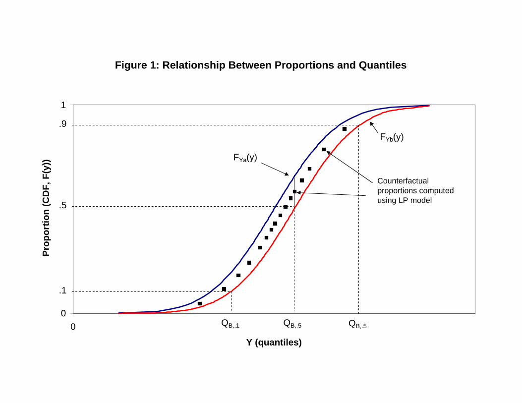
Figure 1: Relationship Between Proportions and Quantiles

0

1

0

Y (quantiles)

Prop

ortio

n (C

DF,

F(y

))

FYb(y)

FYa(y)

QB,.5

.5

.1

QB,.5QB,.1

.9

Counterfactual proportions computed using LP model

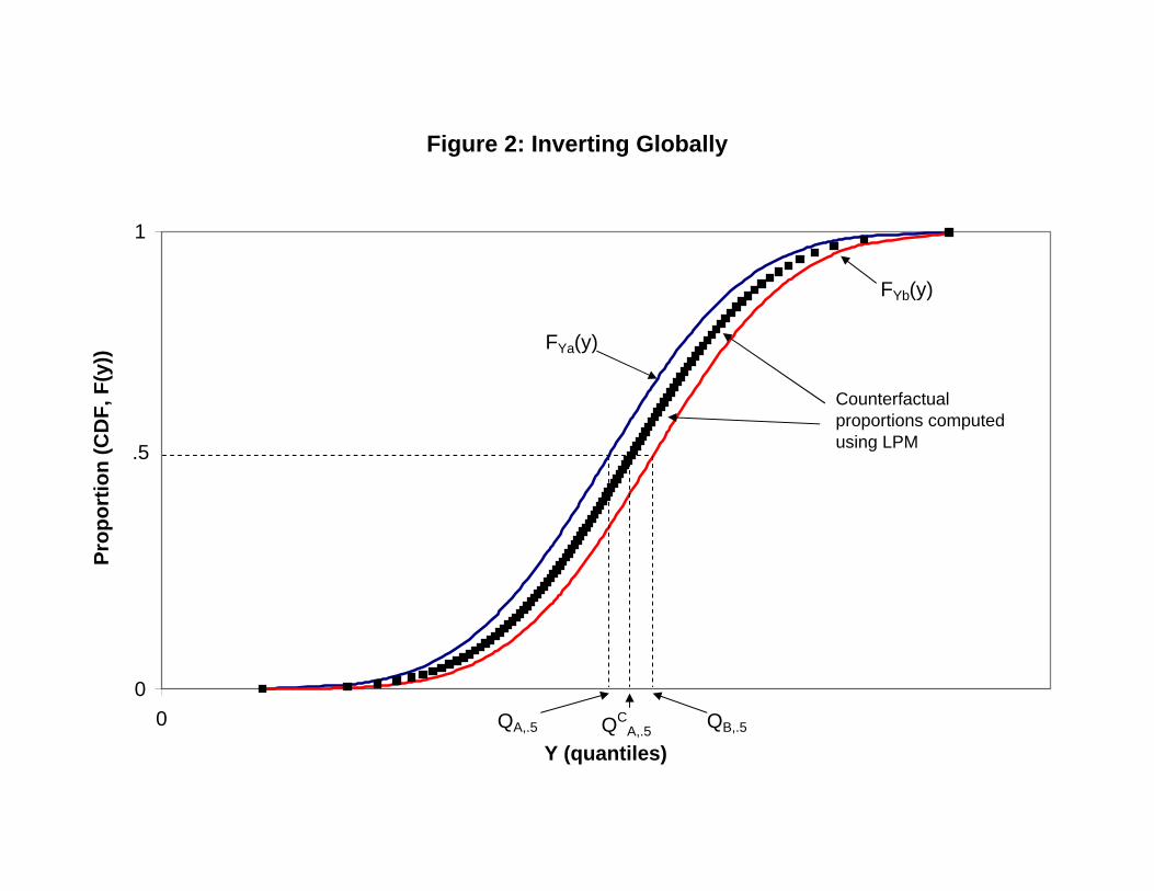
Figure 2: Inverting Globally

0

1

0

Y (quantiles)

Prop

ortio

n (C

DF,

F(y

))

FYb(y)

FYa(y)

QCA,.5

.5

QB,.5QA,.5

Counterfactual proportions computed using LPM

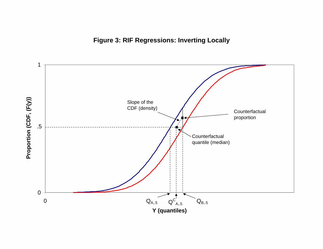
Figure 3: RIF Regressions: Inverting Locally

0

1

0

Y (quantiles)

Prop

ortio

n (C

DF,

(F(y

))

QCA,.5

.5

Counterfactual quantile (median)

QB,.5QA,.5

Counterfactualproportion

Slope of the CDF (density)

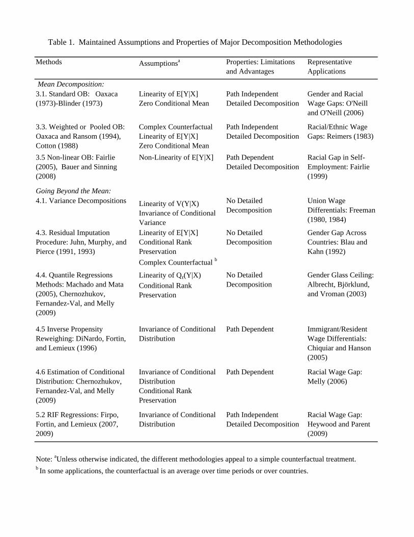
Table 1. Maintained Assumptions and Properties of Major Decomposition Methodologies

Methods Assumptionsa Properties: Limitations and Advantages

Representative Applications

Mean Decomposition:3.1. Standard OB: Oaxaca (1973)-Blinder (1973)

Linearity of E[Y|X] Zero Conditional Mean

Path Independent Detailed Decomposition

Gender and Racial Wage Gaps: O'Neill and O'Neill (2006)

3.3. Weighted or Pooled OB: Oaxaca and Ransom (1994), Cotton (1988)

Complex Counterfactual Linearity of E[Y|X] Zero Conditional Mean

Path Independent Detailed Decomposition

Racial/Ethnic Wage Gaps: Reimers (1983)

3.5 Non-linear OB: Fairlie (2005), Bauer and Sinning (2008)

Non-Linearity of E[Y|X] Path Dependent Detailed Decomposition

Racial Gap in Self-Employment: Fairlie (1999)

Going Beyond the Mean:4.1. Variance Decompositions Linearity of V(Y|X)

Invariance of Conditional Variance

No Detailed Decomposition

Union Wage Differentials: Freeman (1980, 1984)

4.3. Residual Imputation Procedure: Juhn, Murphy, and Pierce (1991, 1993)

Linearity of E[Y|X] Conditional Rank Preservation Complex Counterfactual b

No Detailed Decomposition

Gender Gap Across Countries: Blau and Kahn (1992)

4.4. Quantile Regressions Methods: Machado and Mata (2005), Chernozhukov, Fernandez-Val, and Melly (2009)

Linearity of Qτ(Y|X) Conditional Rank Preservation

No Detailed Decomposition

Gender Glass Ceiling: Albrecht, Björklund, and Vroman (2003)

4.5 Inverse Propensity Reweighing: DiNardo, Fortin, and Lemieux (1996)

Invariance of Conditional Distribution

Path Dependent Immigrant/Resident Wage Differentials: Chiquiar and Hanson (2005)

4.6 Estimation of Conditional Distribution: Chernozhukov, Fernandez-Val, and Melly (2009)

Invariance of Conditional Distribution Conditional Rank Preservation

Path Dependent Racial Wage Gap: Melly (2006)

5.2 RIF Regressions: Firpo, Fortin, and Lemieux (2007, 2009)

Invariance of Conditional Distribution

Path Independent Detailed Decomposition

Racial Wage Gap: Heywood and Parent (2009)

Note: aUnless otherwise indicated, the different methodologies appeal to a simple counterfactual treatment. b In some applications, the counterfactual is an average over time periods or over countries.

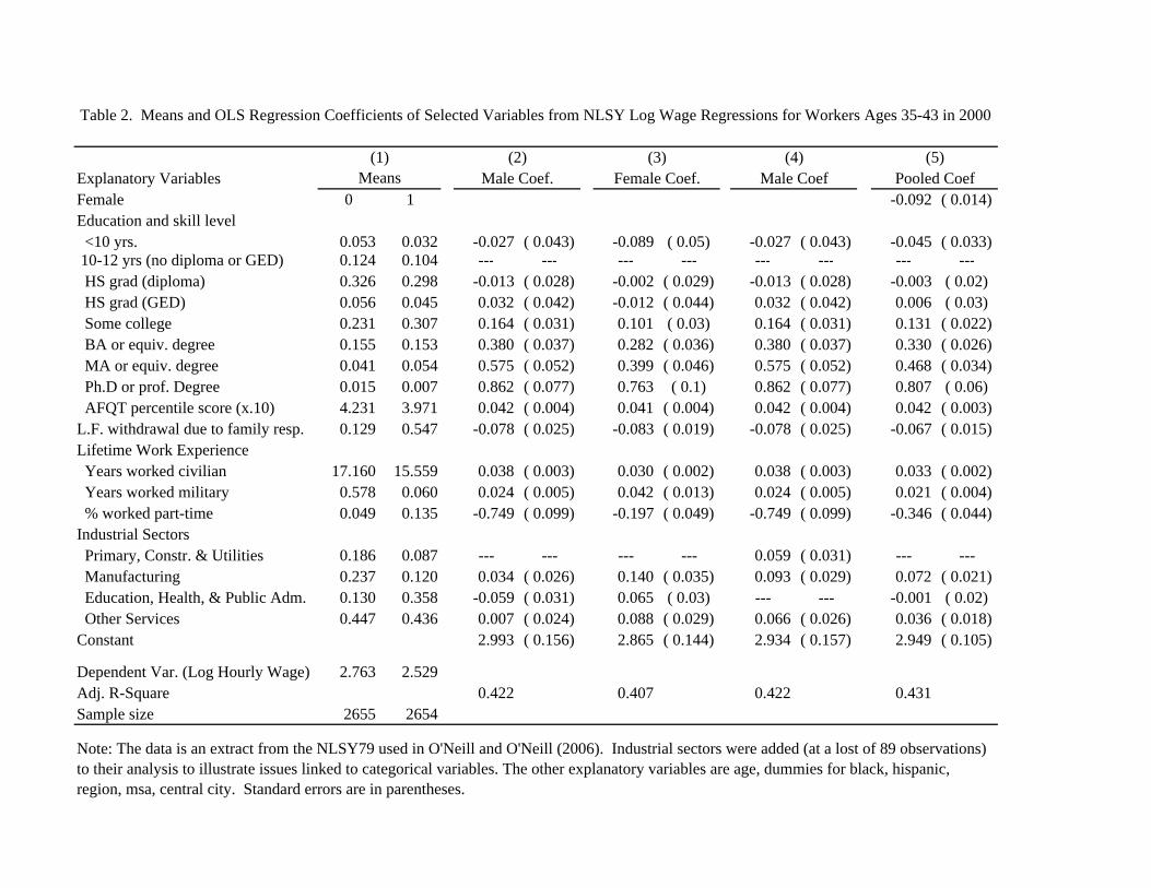
Explanatory VariablesFemale 0 1 -0.092 ( 0.014)Education and skill level <10 yrs. 0.053 0.032 -0.027 ( 0.043) -0.089 ( 0.05) -0.027 ( 0.043) -0.045 ( 0.033) 10-12 yrs (no diploma or GED) 0.124 0.104 --- --- --- --- --- --- --- --- HS grad (diploma) 0.326 0.298 -0.013 ( 0.028) -0.002 ( 0.029) -0.013 ( 0.028) -0.003 ( 0.02) HS grad (GED) 0.056 0.045 0.032 ( 0.042) -0.012 ( 0.044) 0.032 ( 0.042) 0.006 ( 0.03) Some college 0.231 0.307 0.164 ( 0.031) 0.101 ( 0.03) 0.164 ( 0.031) 0.131 ( 0.022) BA or equiv. degree 0.155 0.153 0.380 ( 0.037) 0.282 ( 0.036) 0.380 ( 0.037) 0.330 ( 0.026) MA or equiv. degree 0.041 0.054 0.575 ( 0.052) 0.399 ( 0.046) 0.575 ( 0.052) 0.468 ( 0.034) Ph.D or prof. Degree 0.015 0.007 0.862 ( 0.077) 0.763 ( 0.1) 0.862 ( 0.077) 0.807 ( 0.06) AFQT percentile score (x.10) 4.231 3.971 0.042 ( 0.004) 0.041 ( 0.004) 0.042 ( 0.004) 0.042 ( 0.003)L.F. withdrawal due to family resp. 0.129 0.547 -0.078 ( 0.025) -0.083 ( 0.019) -0.078 ( 0.025) -0.067 ( 0.015)Lifetime Work Experience Years worked civilian 17.160 15.559 0.038 ( 0.003) 0.030 ( 0.002) 0.038 ( 0.003) 0.033 ( 0.002) Years worked military 0.578 0.060 0.024 ( 0.005) 0.042 ( 0.013) 0.024 ( 0.005) 0.021 ( 0.004) % worked part-time 0.049 0.135 -0.749 ( 0.099) -0.197 ( 0.049) -0.749 ( 0.099) -0.346 ( 0.044)Industrial Sectors Primary, Constr. & Utilities 0.186 0.087 --- --- --- --- 0.059 ( 0.031) --- --- Manufacturing 0.237 0.120 0.034 ( 0.026) 0.140 ( 0.035) 0.093 ( 0.029) 0.072 ( 0.021) Education, Health, & Public Adm. 0.130 0.358 -0.059 ( 0.031) 0.065 ( 0.03) --- --- -0.001 ( 0.02) Other Services 0.447 0.436 0.007 ( 0.024) 0.088 ( 0.029) 0.066 ( 0.026) 0.036 ( 0.018)Constant 2.993 ( 0.156) 2.865 ( 0.144) 2.934 ( 0.157) 2.949 ( 0.105)

Dependent Var. (Log Hourly Wage) 2.763 2.529Adj. R-Square 0.422 0.407 0.422 0.431Sample size 2655 2654

Means Female Coef.Male Coef. Male Coef

Table 2. Means and OLS Regression Coefficients of Selected Variables from NLSY Log Wage Regressions for Workers Ages 35-43 in 2000

Pooled Coef

Note: The data is an extract from the NLSY79 used in O'Neill and O'Neill (2006). Industrial sectors were added (at a lost of 89 observations) to their analysis to illustrate issues linked to categorical variables. The other explanatory variables are age, dummies for black, hispanic, region, msa, central city. Standard errors are in parentheses.

(1) (2) (3) (4) (5)

 

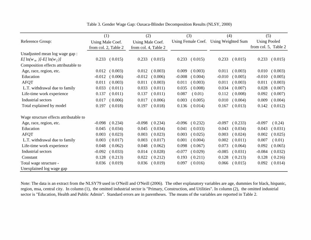
Reference Group:

Unadjusted mean log wage gap : E[ ln(w m )]-E[ ln(w f )] 0.233 ( 0.015) 0.233 ( 0.015) 0.233 ( 0.015) 0.233 ( 0.015) 0.233 ( 0.015)Composition effects attributable to Age, race, region, etc. 0.012 ( 0.003) 0.012 ( 0.003) 0.009 ( 0.003) 0.011 ( 0.003) 0.010 ( 0.003) Education -0.012 ( 0.006) -0.012 ( 0.006) -0.008 ( 0.004) -0.010 ( 0.005) -0.010 ( 0.005) AFQT 0.011 ( 0.003) 0.011 ( 0.003) 0.011 ( 0.003) 0.011 ( 0.003) 0.011 ( 0.003) L.T. withdrawal due to family 0.033 ( 0.011) 0.033 ( 0.011) 0.035 ( 0.008) 0.034 ( 0.007) 0.028 ( 0.007) Life-time work experience 0.137 ( 0.011) 0.137 ( 0.011) 0.087 ( 0.01) 0.112 ( 0.008) 0.092 ( 0.007) Industrial sectors 0.017 ( 0.006) 0.017 ( 0.006) 0.003 ( 0.005) 0.010 ( 0.004) 0.009 ( 0.004) Total explained by model 0.197 ( 0.018) 0.197 ( 0.018) 0.136 ( 0.014) 0.167 ( 0.013) 0.142 ( 0.012)

Wage structure effects attributable to Age, race, region, etc. -0.098 ( 0.234) -0.098 ( 0.234) -0.096 ( 0.232) -0.097 ( 0.233) -0.097 ( 0.24) Education 0.045 ( 0.034) 0.045 ( 0.034) 0.041 ( 0.033) 0.043 ( 0.034) 0.043 ( 0.031) AFQT 0.003 ( 0.023) 0.003 ( 0.023) 0.003 ( 0.025) 0.003 ( 0.024) 0.002 ( 0.025) L.T. withdrawal due to family 0.003 ( 0.017) 0.003 ( 0.017) 0.001 ( 0.004) 0.002 ( 0.011) 0.007 ( 0.01) Life-time work experience 0.048 ( 0.062) 0.048 ( 0.062) 0.098 ( 0.067) 0.073 ( 0.064) 0.092 ( 0.065) Industrial sectors -0.092 ( 0.033) 0.014 ( 0.028) -0.077 ( 0.029) -0.085 ( 0.031) -0.084 ( 0.032) Constant 0.128 ( 0.213) 0.022 ( 0.212) 0.193 ( 0.211) 0.128 ( 0.213) 0.128 ( 0.216)Total wage structure - Unexplained log wage gap

0.036 ( 0.019) 0.036 ( 0.019) 0.097 ( 0.016) 0.066 ( 0.015) 0.092 ( 0.014)

Note: The data is an extract from the NLSY79 used in O'Neill and O'Neill (2006). The other explanatory variables are age, dummies for black, hispanic, region, msa, central city. In column (1), the omitted industrial sector is "Primary, Construction, and Utilities". In column (2), the omitted industrial sector is "Education, Health and Public Admin". Standard errors are in parentheses. The means of the variables are reported in Table 2.

(1) (2) (3) (4) (5)

Table 3. Gender Wage Gap: Oaxaca-Blinder Decomposition Results (NLSY, 2000)

Using Male Coef. from col. 2, Table 2

Using Female Coef. Using Weighted Sum Using Male Coef. from col. 4, Table 2

Using Pooled from col. 5, Table 2

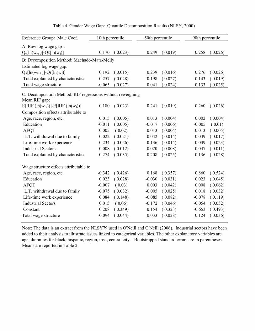
 Reference Group: Male Coef.

A: Raw log wage gap : Qτ[ln(wm )]-Qτ[ln(wf)] 0.170 ( 0.023) 0.249 ( 0.019) 0.258 ( 0.026)

Estimated log wage gap: Qτ[ln(wm )]-Qτ[ln(wf)] 0.192 ( 0.015) 0.239 ( 0.016) 0.276 ( 0.026) Total explained by characteristics 0.257 ( 0.028) 0.198 ( 0.027) 0.143 ( 0.019) Total wage structure -0.065 ( 0.027) 0.041 ( 0.024) 0.133 ( 0.025)

Mean RIF gap: E[RIFτ(ln(wm))]-E[RIFτ(ln(wf))] 0.180 ( 0.023) 0.241 ( 0.019) 0.260 ( 0.026)Composition effects attributable to Age, race, region, etc. 0.015 ( 0.005) 0.013 ( 0.004) 0.002 ( 0.004) Education -0.011 ( 0.005) -0.017 ( 0.006) -0.005 ( 0.01) AFQT 0.005 ( 0.02) 0.013 ( 0.004) 0.013 ( 0.005) L.T. withdrawal due to family 0.022 ( 0.021) 0.042 ( 0.014) 0.039 ( 0.017) Life-time work experience 0.234 ( 0.026) 0.136 ( 0.014) 0.039 ( 0.023) Industrial Sectors 0.008 ( 0.012) 0.020 ( 0.008) 0.047 ( 0.011) Total explained by characteristics 0.274 ( 0.035) 0.208 ( 0.025) 0.136 ( 0.028)

Wage structure effects attributable to Age, race, region, etc. -0.342 ( 0.426) 0.168 ( 0.357) 0.860 ( 0.524) Education 0.023 ( 0.028) -0.030 ( 0.031) 0.023 ( 0.045) AFQT -0.007 ( 0.03) 0.003 ( 0.042) 0.008 ( 0.062) L.T. withdrawal due to family -0.075 ( 0.032) -0.005 ( 0.025) 0.018 ( 0.032) Life-time work experience 0.084 ( 0.148) -0.085 ( 0.082) -0.078 ( 0.119) Industrial Sectors 0.015 ( 0.06) -0.172 ( 0.046) -0.054 ( 0.052) Constant 0.208 ( 0.349) 0.154 ( 0.323) -0.653 ( 0.493)Total wage structure -0.094 ( 0.044) 0.033 ( 0.028) 0.124 ( 0.036)

Table 4. Gender Wage Gap: Quantile Decomposition Results (NLSY, 2000)

10th percentile 50th percentile 90th percentile

Note: The data is an extract from the NLSY79 used in O'Neill and O'Neill (2006). Industrial sectors have been added to their analysis to illustrate issues linked to categorical variables. The other explanatory variables are age, dummies for black, hispanic, region, msa, central city. Bootstrapped standard errors are in parentheses. Means are reported in Table 2.

B: Decomposition Method: Machado-Mata-Melly

C: Decomposition Method: RIF regressions without reweighing

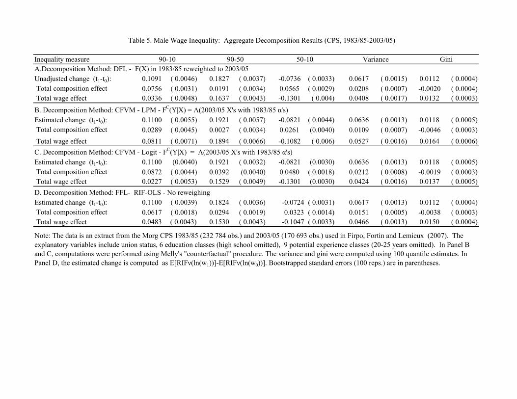
 Inequality measure

Unadjusted change (t1-t0): 0.1091 ( 0.0046) 0.1827 ( 0.0037) -0.0736 ( 0.0033) 0.0617 ( 0.0015) 0.0112 ( 0.0004) Total composition effect 0.0756 ( 0.0031) 0.0191 ( 0.0034) 0.0565 ( 0.0029) 0.0208 ( 0.0007) -0.0020 ( 0.0004) Total wage effect 0.0336 ( 0.0048) 0.1637 ( 0.0043) -0.1301 ( 0.004) 0.0408 ( 0.0017) 0.0132 ( 0.0003)

Estimated change (t1-t0): 0.1100 ( 0.0055) 0.1921 ( 0.0057) -0.0821 ( 0.0044) 0.0636 ( 0.0013) 0.0118 ( 0.0005) Total composition effect 0.0289 ( 0.0045) 0.0027 ( 0.0034) 0.0261 (0.0040) 0.0109 ( 0.0007) -0.0046 ( 0.0003) Total wage effect 0.0811 ( 0.0071) 0.1894 ( 0.0066) -0.1082 ( 0.006) 0.0527 ( 0.0016) 0.0164 ( 0.0006)

Estimated change (t1-t0): 0.1100 (0.0040) 0.1921 ( 0.0032) -0.0821 (0.0030) 0.0636 ( 0.0013) 0.0118 ( 0.0005) Total composition effect 0.0872 ( 0.0044) 0.0392 (0.0040) 0.0480 ( 0.0018) 0.0212 ( 0.0008) -0.0019 ( 0.0003) Total wage effect 0.0227 ( 0.0053) 0.1529 ( 0.0049) -0.1301 (0.0030) 0.0424 ( 0.0016) 0.0137 ( 0.0005)

Estimated change (t1-t0): 0.1100 ( 0.0039) 0.1824 ( 0.0036) -0.0724 ( 0.0031) 0.0617 ( 0.0013) 0.0112 ( 0.0004) Total composition effect 0.0617 ( 0.0018) 0.0294 ( 0.0019) 0.0323 ( 0.0014) 0.0151 ( 0.0005) -0.0038 ( 0.0003) Total wage effect 0.0483 ( 0.0043) 0.1530 ( 0.0043) -0.1047 ( 0.0033) 0.0466 ( 0.0013) 0.0150 ( 0.0004)

         

50-10 VarianceA.Decomposition Method: DFL - F(X) in 1983/85 reweighted to 2003/05

D. Decomposition Method: FFL- RIF-OLS - No reweighing

B. Decomposition Method: CFVM - LPM - FC(Y|X) = Λ(2003/05 X's with 1983/85 α's)

C. Decomposition Method: CFVM - Logit - FC(Y|X) = Λ(2003/05 X's with 1983/85 α's)

Note: The data is an extract from the Morg CPS 1983/85 (232 784 obs.) and 2003/05 (170 693 obs.) used in Firpo, Fortin and Lemieux (2007). The explanatory variables include union status, 6 education classes (high school omitted), 9 potential experience classes (20-25 years omitted). In Panel B and C, computations were performed using Melly's "counterfactual" procedure. The variance and gini were computed using 100 quantile estimates. In Panel D, the estimated change is computed as E[RIFν(ln(w1))]-E[RIFν(ln(w0))]. Bootstrapped standard errors (100 reps.) are in parentheses.

Table 5. Male Wage Inequality: Aggregate Decomposition Results (CPS, 1983/85-2003/05)

Gini90-10 90-50

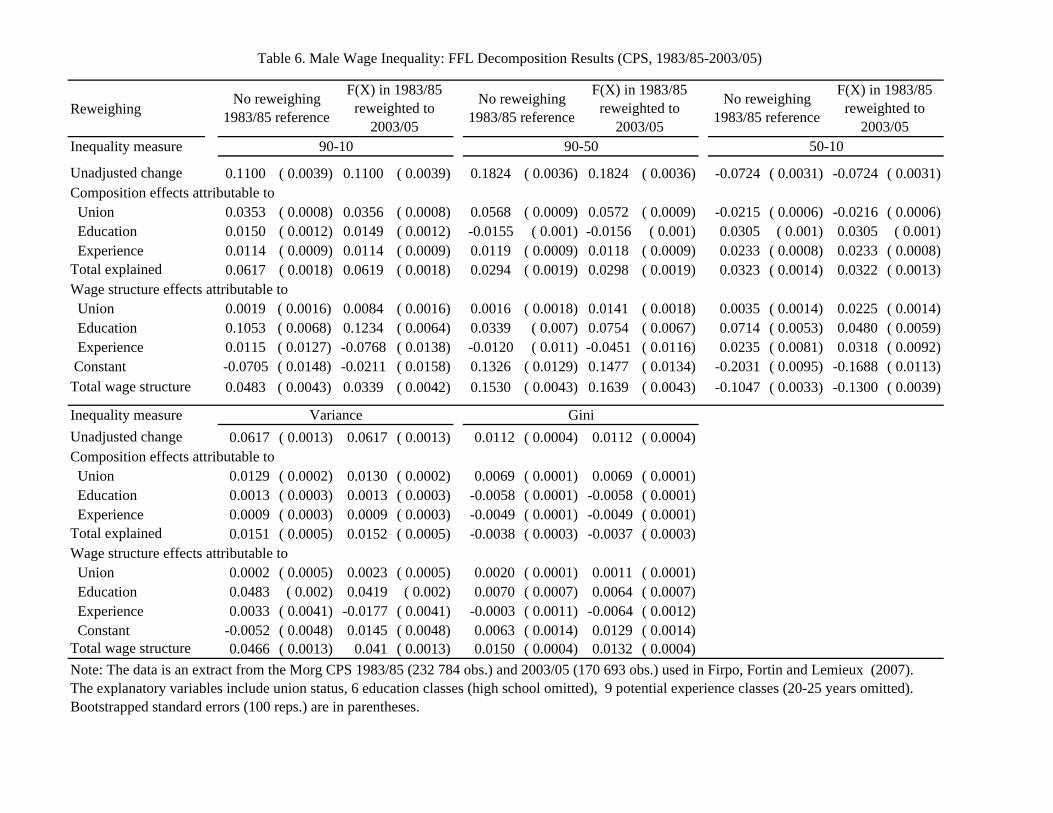
Reweighing

Inequality measure

Unadjusted change 0.1100 ( 0.0039) 0.1100 ( 0.0039) 0.1824 ( 0.0036) 0.1824 ( 0.0036) -0.0724 ( 0.0031) -0.0724 ( 0.0031)Composition effects attributable to Union 0.0353 ( 0.0008) 0.0356 ( 0.0008) 0.0568 ( 0.0009) 0.0572 ( 0.0009) -0.0215 ( 0.0006) -0.0216 ( 0.0006) Education 0.0150 ( 0.0012) 0.0149 ( 0.0012) -0.0155 ( 0.001) -0.0156 ( 0.001) 0.0305 ( 0.001) 0.0305 ( 0.001) Experience 0.0114 ( 0.0009) 0.0114 ( 0.0009) 0.0119 ( 0.0009) 0.0118 ( 0.0009) 0.0233 ( 0.0008) 0.0233 ( 0.0008)Total explained 0.0617 ( 0.0018) 0.0619 ( 0.0018) 0.0294 ( 0.0019) 0.0298 ( 0.0019) 0.0323 ( 0.0014) 0.0322 ( 0.0013)Wage structure effects attributable to Union 0.0019 ( 0.0016) 0.0084 ( 0.0016) 0.0016 ( 0.0018) 0.0141 ( 0.0018) 0.0035 ( 0.0014) 0.0225 ( 0.0014) Education 0.1053 ( 0.0068) 0.1234 ( 0.0064) 0.0339 ( 0.007) 0.0754 ( 0.0067) 0.0714 ( 0.0053) 0.0480 ( 0.0059) Experience 0.0115 ( 0.0127) -0.0768 ( 0.0138) -0.0120 ( 0.011) -0.0451 ( 0.0116) 0.0235 ( 0.0081) 0.0318 ( 0.0092) Constant -0.0705 ( 0.0148) -0.0211 ( 0.0158) 0.1326 ( 0.0129) 0.1477 ( 0.0134) -0.2031 ( 0.0095) -0.1688 ( 0.0113)Total wage structure 0.0483 ( 0.0043) 0.0339 ( 0.0042) 0.1530 ( 0.0043) 0.1639 ( 0.0043) -0.1047 ( 0.0033) -0.1300 ( 0.0039)

Inequality measureUnadjusted change 0.0617 ( 0.0013) 0.0617 ( 0.0013) 0.0112 ( 0.0004) 0.0112 ( 0.0004)Composition effects attributable to Union 0.0129 ( 0.0002) 0.0130 ( 0.0002) 0.0069 ( 0.0001) 0.0069 ( 0.0001) Education 0.0013 ( 0.0003) 0.0013 ( 0.0003) -0.0058 ( 0.0001) -0.0058 ( 0.0001) Experience 0.0009 ( 0.0003) 0.0009 ( 0.0003) -0.0049 ( 0.0001) -0.0049 ( 0.0001)Total explained 0.0151 ( 0.0005) 0.0152 ( 0.0005) -0.0038 ( 0.0003) -0.0037 ( 0.0003)Wage structure effects attributable to Union 0.0002 ( 0.0005) 0.0023 ( 0.0005) 0.0020 ( 0.0001) 0.0011 ( 0.0001) Education 0.0483 ( 0.002) 0.0419 ( 0.002) 0.0070 ( 0.0007) 0.0064 ( 0.0007) Experience 0.0033 ( 0.0041) -0.0177 ( 0.0041) -0.0003 ( 0.0011) -0.0064 ( 0.0012) Constant -0.0052 ( 0.0048) 0.0145 ( 0.0048) 0.0063 ( 0.0014) 0.0129 ( 0.0014)Total wage structure 0.0466 ( 0.0013) 0.041 ( 0.0013) 0.0150 ( 0.0004) 0.0132 ( 0.0004)

Table 6. Male Wage Inequality: FFL Decomposition Results (CPS, 1983/85-2003/05)

90-10 90-50 50-10

Variance Gini

Note: The data is an extract from the Morg CPS 1983/85 (232 784 obs.) and 2003/05 (170 693 obs.) used in Firpo, Fortin and Lemieux (2007). The explanatory variables include union status, 6 education classes (high school omitted), 9 potential experience classes (20-25 years omitted). Bootstrapped standard errors (100 reps.) are in parentheses.

No reweighing 1983/85 reference

No reweighing 1983/85 reference

F(X) in 1983/85 reweighted to

2003/05

F(X) in 1983/85 reweighted to

2003/05

No reweighing 1983/85 reference

F(X) in 1983/85 reweighted to

2003/05