11/5/2013

1

Decomposition Methods: The Case of Mean and Beyond

Nicole M Fortin, UBCSpecial LectureDepartment of Economics, Yale University

Lecture on Decomposition Methods

Relies heavily on the chapter “Decomposition Methods in Economics” (joint with Thomas Lemieux and Sergio Firpo) in the recent Handbook of Labor Economics (Volume 4A, 2011)

Uses the classic work of Oaxaca (1973) and Blinder (1973) for the meanas its point of departure

Focuses on recent developments (last 15 years) on how to go beyond the mean Connection with the treatment effect literature Procedures specific to the case of decompositions

Provides some examples to motivate the use of decomposition methods Provides empirical illustrations and discusses applications Suggests a “user guide” of best practices

Plan for the first part

Introduction A few motivating examples Oaxaca decompositions: a refresher Issues involved when going “beyond the mean”

A formal theory of decompositions Clarify the question being asked Decompositions as counterfactual exercises Formal connection with the treatment effect literature:

Identification: the central role of the ignorability (or unconfoundedness) assumption

Estimators for the “aggregate” decomposition: propensity score matching, reweighting, etc.

Introduction: motivating examples

1. Gender wage gap (Oaxaca-Blinder) Construction of counterfactuals

2. Union wage gap Link to the treatment effects literature

3. Understanding changes in wage inequality The case for going beyond the mean

11/5/2013

2

Gender Wage Gap Oaxaca (1973) was the first study (along with Blinder, 1973) aimed

at understanding the sources of the large gender gap in wage. Gender gap (difference between male and female average wages)

of 43 percent in the 1967 Survey of Economics Opportunity Question: how much of the gender gap can be “explained” by male-

female differences in human capital (education and labor market experience), occupational choices, etc? The “unexplained” part of the gender gap is often interpreted as representing

labor market discrimination, though other interpretations(unobserved skills) are possible too

Estimate OLS regressions of (log) wages on covariates/characteristics/endowments

Use the estimates to construct a counterfactual wage such as “what would be the average wage of women if they had the same characteristics as men?”

Glass ceiling effects give a case for of going beyond the case

•If the proportion of men across ranks was identical to women, the overall counterfactual average male salary would be: 31/100×152493.4 + 43.9/100×121483.4 + 25.1/100×106805.6 =127426.43, and the overall ratio would be 120623.1/127426.43 (*100)= 94.66%. • If the proportion of women across rank was identical to men, the overall counterfactual average female salary would be: 51.8/100×146047.5 + 30.7/100×114594.9 + 17.6/100×99708.87 =128259.3, and the overall ratio would be 134955.3/128259.3(*100)=95.03%. •Either way, more than 50% of the gap is accounted for by the gender differences in the proportion of faculty members across rank.

Table 1. Average Professorial Salaries at UBC in 2010

Gender Rank Numbers % of All

% of women

Average Salary

Female/ Male Ratio

Men All 968 100.0 134955.3 0.89 Women All 419 100.0 30.2 120623.1 Men Full 501 51.8 152493.4 0.96 Women Full 130 31.0 20.6 146047.5 Men Associate 297 30.7 121483.4 0.94 Women Associate 184 43.9 38.3 114594.9 Men Assistant 170 17.6 106805.6 0.93 Women Assistant 105 25.1 38.2 99708.87

Union Wage Gap Workers covered by collective bargaining agreement (minority of

workers in Canada, the U.S. or U.K.), or “union workers”, earn more on average than other workers.

One can do a Oaxaca-type decomposition to separate the “true” union effect from differences in characteristics between union and nonunion workers. The “unexplained” part of the decomposition is now the union effect.

Unlike the case of the gender wage gap, we can think of the union effect as a treatment effect since union status is manipulable (can in principle be switched on and off for a given worker)

Useful since tools and results from the treatment effect literature can be used in the context of this decomposition.

Results from the treatment effect can also be used in cases where the group indicator is not manipulable (e.g. men vs. women)

Classic example of variance decomposition!Source: Fortin and Lemieux (1997)

11/5/2013

3

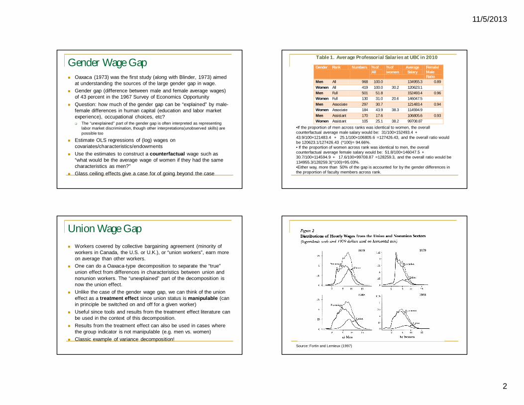
Changes in Wage Inequality Wage/earnings inequality has increased in many countries over the

last 30 years; in the 1990s we saw a polarization of earnings Decomposition methods have been used to look for explanations for

these changes, such as: Decline in unions and in the minimum wage Increase in the rate of return to education Technological change, international competition, etc.

We need to go “beyond the mean” which is more difficult than performing a standard Oaxaca decomposition for the mean.

Active area of research over the last 20 years. A number of procedures are now available, a few examples: Juhn, Murphy, and Pierce (1993): Imputation method DiNardo, Fortin, and Lemieux (1996): Reweighting method Machado and Mata (2005): Quantile regression-based method

-.2-.1

0.1

.2Lo

g W

age

Diff

eren

tial

0 .2 .4 .6 .8 1Quantile

Observed 1988/90-1976/78SmoothedObserved 2000/02-1988/90Smoothed

Figure 1. Changes in Real ($1979) Log Male Wages by Percentiles –MORG-CPS

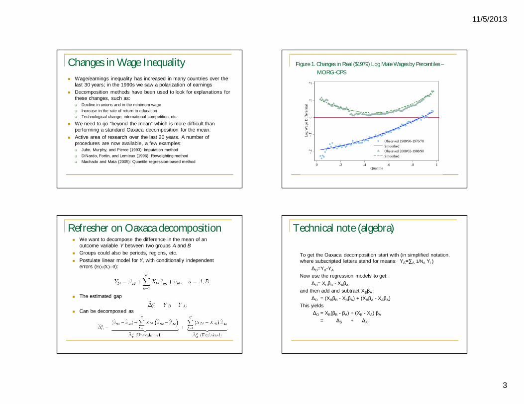
Refresher on Oaxaca decomposition We want to decompose the difference in the mean of an

outcome variable Y between two groups A and B Groups could also be periods, regions, etc. Postulate linear model for Y, with conditionally independent

errors (E(υ|X)=0):

The estimated gap

Can be decomposed as

Technical note (algebra)

To get the Oaxaca decomposition start with (in simplified notation, where subscripted letters stand for means: YA=∑A 1/NA Yi )

ΔO=YB-YA

Now use the regression models to get:ΔO= XBβB - XAβA

and then add and subtract XBβA :ΔO = (XBβB - XBβA) + (XBβA - XAβA)

This yieldsΔO = XB(βB - βA) + (XB - XA) βA

= ΔS + ΔX

11/5/2013

4

Some terminology The lecture focuses on wage decompositions The “explained” part of the decomposition will be called the

composition effect since it reflects differences in the distribution of the X’s between the two groups

The “unexplained” part of the decomposition will be called the wage structure effect as it reflects differences in the β’s, i.e. in the way the X’s are “priced” (or valued) in the labor market.

Studies sometimes refer to “price” (β’s) and “quantity” (X’s) effects instead.

In the “aggregate” decomposition, we only divide Δ into its two components ΔS (wage structure effect) and ΔX (composition effect).

In the “detailed” decomposition we also look at the contribution of each individual covariate (or corresponding β)

A few remarks We focus on this particular decomposition, but we could also change

the reference wage structure

Or add an interaction term:

Does not affect the substance of the argument in most cases. The “intercept” component of ΔS, βB0- βA0, is the wage structure

effect for the base group. Unless the other β’s are the same in group A and B, βB0- βA0 will arbitrarily depend on the base group chosen.

Well known problem, e.g. Oaxaca and Ransom (1999).

Oaxaca decompositions in Stata

Main command is “oaxaca.ado” (due to Ben Jann, U of Zurich, has to be downloaded)

Runs the regressions, computes the means, and computes the elements of the decomposition along with standard errors (see A Stata implementation of the Blinder-Oaxaca decomposition)

We provide all the programs used to produce the tables in the Handbook chapter at: http://faculty.arts.ubc.ca/nfortin/datahead.html

Here is an example of how this works for a standard male-female decomposition (Table 3 in our Handbook chapter from O’Neill and O’Neill (2006) using data from the NLSY79 in 2000) *** Table 3, Column 1;

oaxaca lropc00 age00 msa ctrlcity north_central south00 west hispanic black sch_10 diploma_hs ged_hs smcol bachelor_colmaster_col doctor_col afqtp89 famrspb wkswk_18 yrsmil78_00 pcntpt_22 manuf eduheal othind,by(female) weight(1)

/*weight(1) uses the group 1 coefficients as the reference coefficients, and weight(0) uses the group 2 coefficients */

detail(groupdem:age00 msa ctrlcity north_central south00 west hispanic black,groupaf:afqtp89,

grouped:sch_10 diploma_hs ged_hs smcol bachelor_colmaster_col doctor_col ,groupfam:famrspb,

groupex:wkswk_18 yrsmil78_00 pcntpt_22 ,groupind: manuf eduheal othind) ;

Here the base group is white, sch10-12, primary sector,

11/5/2013

5

Blinder-Oaxaca decomposition Number of obs = 5309

1: female = 02: female = 1

------------------------------------------------------------------------------lropc00 | Coef. Std. Err. z P>|z| [95% Conf. Interval]

-------------+----------------------------------------------------------------Differential |Prediction_1 | 2.762557 .0106598 259.16 0.000 2.741664 2.78345Prediction_2 | 2.529257 .0100367 252.00 0.000 2.509585 2.548928

Difference | .2333003 .0146413 15.93 0.000 .2046039 .2619967-------------+----------------------------------------------------------------Explained |

groupdem | .0115371 .0032919 3.50 0.000 .0050851 .0179891grouped | -.0124049 .0055175 -2.25 0.025 -.023219 -.0015907groupaf | .0108035 .0034414 3.14 0.002 .0040584 .0175486

groupfam | .0328186 .0106373 3.09 0.002 .0119698 .0536674groupex | .137095 .0112599 12.18 0.000 .1150259 .159164

groupind | .0174583 .0061707 2.83 0.005 .005364 .0295526Total | .1973076 .0180079 10.96 0.000 .1620128 .2326024

-------------+----------------------------------------------------------------Unexplained |

groupdem | -.0978872 .2338861 -0.42 0.676 -.5562956 .3605212grouped | .0454348 .0344576 1.32 0.187 -.0221009 .1129705groupaf | .0026284 .023485 0.11 0.911 -.0434014 .0486582

groupfam | .0025869 .0174562 0.15 0.882 -.0316266 .0368005groupex | .0475104 .0616535 0.77 0.441 -.0733281 .168349

groupind | -.0920156 .03294 -2.79 0.005 -.1565769 -.0274543_cons | .1277349 .2127739 0.60 0.548 -.2892944 .5447641Total | .0359927 .0185897 1.94 0.053 -.0004425 .0724279

------------------------------------------------------------------------------

Problems when going beyond the mean The case of the mean is simple because we can use the law of

conditional expectations, and then plug-in sample estimates

In non-linear models, things are also more complicated

11/5/2013

6

Problems when going beyond the mean Things get more complicated in cases such as the variance Using the analysis of variance formula, we can write the

unconditional variance as

So that the decomposition, where , has to include interactions terms between the covariates,

And could become even more complicated for more general distributional statistics such as quantiles, the Gini coefficient, etc.

Back to identification: what can we estimate using decompositions? Computing a Oaxaca decomposition is easy enough

Run OLS and compute mean values of X for each of the two groups In Stata, “oaxaca.ado” does that automatically and also yields standard

errors that reflect the fact both the β’s and the mean values of the X’s are being estimated.

But practitioners often wonder what we are really estimating for the following reasons (to list a few): What if some the X variables (e.g. years of education) are endogenous? What if there is some selection between (e.g. choice of being unionized or not) or

within (participation rates for men and women) the two groups under consideration?

What about general equilibrium effects? For example if we increase the level of human capital (say experience) of women to the level of men, this may depress the return to experience and invalidate the decomposition

Key question: Can we construct a valid counterfactual?

Recall that decompositions are based on counterfactuals

Recall that we can write:ΔO=YB-YA=(YB-YC) + (YC-YA),

where YC is the counterfactual wage members of group B (say women) would earn if they were paid like men (group A). Under the linearity assumption (of the regression model), we get:

YA= XAβA, YB= XBβB, and YC= XBβA.We then obtain the Oaxaca decomposition as follows:

ΔO = (XBβB - XBβA) + (XBβA - XAβA)= XB(βB - βA) + βA(XB - XA)= ΔS + ΔX

So with an estimate of the counterfactual YC one can compute the decomposition. This is a general point that holds for all decompositions, and not only for the mean

Counterfactual and treatment effects Generally speaking, one can think of treatment effects as the

difference between how people are actually paid, and how they would be paid under a different “treatment”.

Take the case of unions. YA : Average wage of non-union workers YB : Average wage of union workers YC : Counterfactual wage union members would earn if the were not

unionized ΔS = YB-YC = “union effect” on union workers is an average treatment

effect on the treated (ATET) This means that the identification/estimation issue involved in the

case of decomposition/counterfactual are the same as in the case of treatment effects.

This is very useful since we can then use results from the treatment effect literature.

11/5/2013

7

The wage structure effect (ΔS) can be interpreted as a treatment effect

The conditional independence assumption (E(ε|X)=0) usually invoked in Oaxaca decompositions can be replaced by the weaker ignorability assumption (Dg ╨ ε|X) to compute the aggregate decomposition

For example, ability (ε) can be correlated with education (X) as long as the correlation is the same in groups A and B.

This is the standard assumption used in “selection on observables” models where matching methods are typically used to estimate the treatment effect.

Main result: If we have YG=mG(X, ε) and ignorability, then: ΔS solely reflects changes in the m(.) functions (ATET) ΔX solely reflects changes in the distribution of X and ε

(ignorability key for this last result).

The wage structure effect (ΔS) can be interpreted as a treatment effect A number of estimators for ATET= ΔS have been proposed in the

treatment effect literature Inverse probability weighting (IPW), matching, etc.

Formal results exist, e.g. IPW is efficient for ATET (Hirano, Imbens, and Ridder, 2003) Quantile treatment effects (Firpo, 2007)

This has been widely used in the decomposition literature since DiNardo, Fortin, and Lemieux (1996).

Formal derivation of the identification result (Handbook chapter)

Formal derivation (2)

11/5/2013

8

Formal derivation (3) Some intuition about Proposition 1 The wage setting model we use, Yg =mg (X,ε) is very general

Includes the linear model yg = xβg + ε as a special case There are three reasons why wages can be different between

groups g=A and g=B: Differences in the wage setting equations ma (.) and mb (.) Differences in the distribution of X for the two groups Differences in the distribution of ε for the two groups

The ignorability assumption states that the distribution of ε given X is the same for the two groups, though this does not mean that E(ε|X)=0.

So once we control for differences between the X’s in the two groups, we also implicitly control for differences in the ε’s.

Only source of difference left is, thus, differences in the wage structures ma (.) and mb (.).

A few caveats discussed in the chapter

This general result (Proposition 1) only works for the aggregate decomposition. More assumptions have to be imposed to get at the detailed decomposition.

We are implicitly ruling out general equilibrium effects under assumption (simple counterfactual treatment).

For instance, in the absence of unions, wages in the nonunionsector may change as firms are no longer confronted with the threat of unionization

The wage structure observed among nonunion workers, ma (.), is no longer a valid counterfactual for union workers.

This is closely related to the difference between union wage gap (no general equilibrium effects) and union wage gain (possible general equilibrium effects) discussed by H. Gregg Lewis decades ago

Plan for the second part: Going beyond the mean Examples of distributional questions Quantile regressions: analogy with standard regressions

doesn’t work Constructing counterfactual distributions Aggregate decomposition: reweighting procedure Detailed decomposition:

Conditional reweighting Quantile regression based decomposition (Machado-Mata) Distributional regressions (Chernozhukov et al.) RIF-regression (Firpo, Fortin, and Lemieux)

Empirical application and implementation in Stata

11/5/2013

9

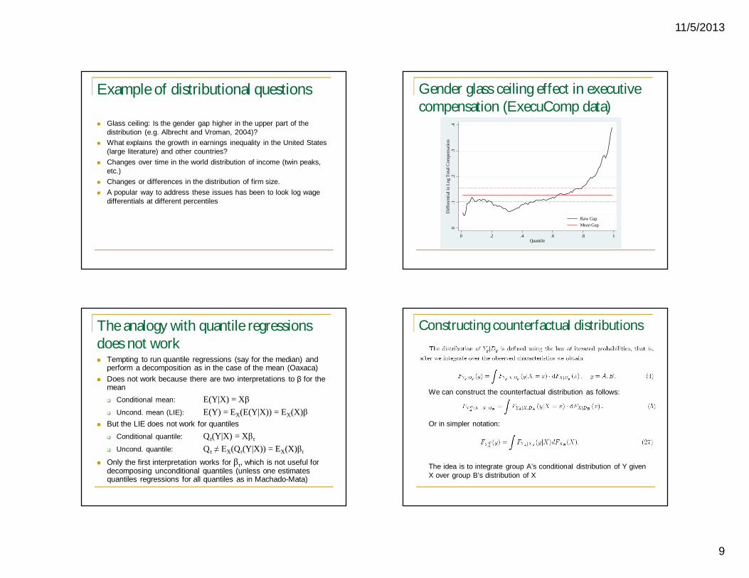
Example of distributional questions

Glass ceiling: Is the gender gap higher in the upper part of the distribution (e.g. Albrecht and Vroman, 2004)?

What explains the growth in earnings inequality in the United States (large literature) and other countries?

Changes over time in the world distribution of income (twin peaks, etc.)

Changes or differences in the distribution of firm size. A popular way to address these issues has been to look log wage

differentials at different percentiles

0.1

.2.3

.4D

iffer

entia

l in

Log

Tota

l Com

pens

atio

n

0 .2 .4 .6 .8 1Quantile

Raw GapMean Gap

Gender glass ceiling effect in executive compensation (ExecuComp data)

The analogy with quantile regressions does not work Tempting to run quantile regressions (say for the median) and

perform a decomposition as in the case of the mean (Oaxaca) Does not work because there are two interpretations to β for the

mean Conditional mean: E(Y|X) = Xβ Uncond. mean (LIE): E(Y) = EX(E(Y|X)) = EX(X)β

But the LIE does not work for quantiles Conditional quantile: Qτ(Y|X) = Xβτ

Uncond. quantile: Qτ ≠ EX(Qτ(Y|X)) = EX(X)βτ

Only the first interpretation works for βτ, which is not useful for decomposing unconditional quantiles (unless one estimates quantiles regressions for all quantiles as in Machado-Mata)

Constructing counterfactual distributions

We can construct the counterfactual distribution as follows:

Or in simpler notation:

The idea is to integrate group A’s conditional distribution of Y given X over group B’s distribution of X

11/5/2013

10

Constructing counterfactual distributions There are two general ways of estimating the counterfactual

distribution First approach is to start with group B and replace the conditional

distribution FYB|XB(y|X) with FYA|XA(y|X) This requires estimating the whole conditional distribution. Machado and Mata (2005) do so by estimating quantile

regressions for all quantiles, and inverting back Second approach is the opposite. Start with group A but replace the

distribution of X for group A (FXA(X)) by the distribution of X for group B (FXB(X)).

This is simpler since this only depends on X, while the conditional distribution depends on both X and Y.

Even better, all we need to do is to compute a reweighting factor

Constructing counterfactual distributions

This is the approach suggested by DiNardo, Fortin and Lemieux (1996)

The reweighting factor can be estimated using a simple logit (or probit) model since after some manipulations we get

To estimate Prob(DB=1|X), pool the two groups and estimate a logit for the probability of belonging to group B as a function of X

Reweighting procedure Reweighting procedure: a few lines of code*include a lot of non-linear interactions;

local edvar "sch_10 diploma_hs ged_hs smcol bachelor_col master_coldoctor_col";

foreach kv of local edvar {;

gen `kv'afqt=`kv‘*afqtp89; gen `kv'exp=`kv'*wkswk_18; }; gen expafqt=afqtp89*wkswk_18; gen expsq=wkswk_18^2;

gen yrsmilsq=yrsmil78_00^2;

***probit for male;

probit male age00 msa ctrlcity north_central south00 west hispanic black schl00 sch_10* diploma_hs* ged_hs* smcol* bachelor_col* master_col* doctor_col* afqtp89 expafqt wkswk_18 expsq yrsmil78_00 yrsmilsqpcntpt_22 manuf eduheal othind if female==0 | female==1 ;

predict pmale, p;

*/ top code weights if necessary */

summ pmale if male~=1, detail;

replace pmale=0.99 if pmale>0.99 & male~=1;gen phix=(pmale)/(1-pmale)*((1-pbar)/pbar) if female==2;

11/5/2013

11

Reweighting procedure

Very easy to use regardless of the distribution statistics being considered (variance, Gini coefficient, inter-quartile range, etc.)

Just compute the statistic for group A, group B, and group A reweighted to have the distribution of X of group B.

Example: in the case of the Gini coefficient, this yields estimates of GiniA, GiniB, and GiniAC

We can then estimate the composition effect as:ΔX = GiniAC - GiniA

And the wage structure effect as ΔS = GiniB – GiniAC

Standard errors can be computed using a bootstrap procedure (bootstrap the whole procedure starting with the logit or probit)

Going beyond the mean is a “solved” problem for the aggregate decomposition Can directly apply non-parametric methods (reweighting, matching,

etc.) from the treatment effect literature. Ignorability is crucial, but mG(X, ε) does not need to be linear Inference by bootstrap or analytical standard errors in the case of

reweighting (“generated regressor” correction required) Reweighting very easy to use with large and well behaved (no

support problem) data sets. Occasionally top-coding weight may be needed Good idea to check the fit!

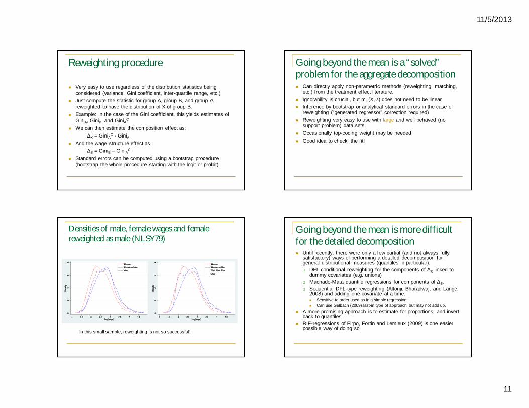
Densities of male, female wages and female reweighted as male (NLSY79)

In this small sample, reweighting is not so successful!

Going beyond the mean is more difficult for the detailed decomposition Until recently, there were only a few partial (and not always fully

satisfactory) ways of performing a detailed decomposition for general distributional measures (quantiles in particular): DFL conditional reweighting for the components of ΔX linked to

dummy covariates (e.g. unions) Machado-Mata quantile regressions for components of ΔS. Sequential DFL-type reweighting (Altonji, Bharadwaj, and Lange,

2008) and adding one covariate at a time. Sensitive to order used as in a simple regression. Can use Gelbach (2009) last-in type of approach, but may not add up.

A more promising approach is to estimate for proportions, and invert back to quantiles.

RIF-regressions of Firpo, Fortin and Lemieux (2009) is one easier possible way of doing so

11/5/2013

12

Going beyond the mean is more difficult for the detailed decomposition We also propose a more general conditional reweighting approach Intuition for components of ΔX:

When sequentially adding regressors, the effect for the last one is consistent since all other covariates have been controlled for.

Similarly, comparing the effect obtained by reweighting on all X’s vs. all X’s except Xk gives the correct effect of Xk.

Repeating the procedure for each Xk gives the right marginal contribution of each Xk, though the k effects do not sum up to the total (interaction effects).

A reweighting approach can also be used to compute the components of ΔS (as in DiNardo and Lemieux, 1997): Restrict sample to Xk=0 (or other base group value) Reweight on the X-k other covariates to have the same distribution

as in the full sample. Gives the distribution when the wage structure effect of Xk has been

set to zero.

Decomposing proportions is easier than decomposing quantiles Easy to do a decomposition by running LP models for the

probability of earning less (or more) than say $17/hrs, and compute a Oaxaca counterfactual on the proportions:

We may find 50% of men earn more than $17/hrs, while only 35% of women do, but if women “were paid as men”, perhaps 45% of women would earn more than $17/hrs

By contrast, much less obvious how to decompose the difference between the 50th quantile for men ($17/hrs) and women (say $14/hrs)

But the function linking proportions and quantiles is the cumulative distribution.

Counterfactual proportions → Counterfactual cumulative → Counterfactual quantiles

Can be illustrated graphically

Figure 1: Relationship Between Proportions and Quantiles

0

1

0 4

Y (quantiles)

Prop

ortio

n (c

umul

. pro

b. (F

(Y))

Men (A)

Women (B)

Q.5

.5

.1

Q.9Q.1

.9

Counterfactual proportions computed using LP model

Figure 3: Inverting Globally

0

1

0 4

Y (quantiles)

Prop

ortio

n (c

umul

. Pro

b. (F

(Y))

Men (A)

Women (B)

Q.5

.5

.1

Q.9Q.1

.9

Counterfactual proportions computed using LP model

11/5/2013

13

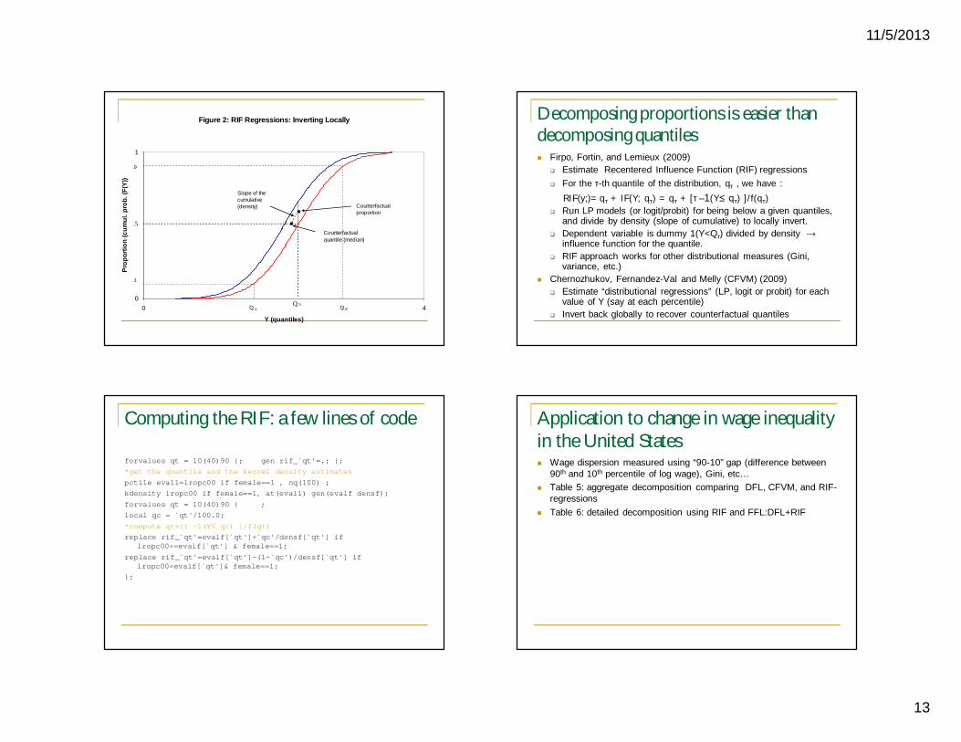
Figure 2: RIF Regressions: Inverting Locally

0

1

0 4

Y (quantiles)

Prop

ortio

n (c

umul

. pro

b. (F

(Y))

Q.5

.5Counterfactual quantile (median)

.1

Q.9Q.1

.9

Counterfactualproportion

Slope of the cumulative(density)

Decomposing proportions is easier than decomposing quantiles Firpo, Fortin, and Lemieux (2009)

Estimate Recentered Influence Function (RIF) regressions For the τ-th quantile of the distribution, qτ , we have :

RIF(y;)= qτ + IF(Y; qτ) = qτ + [τ –1(Y≤ qτ) ]/f(qτ) Run LP models (or logit/probit) for being below a given quantiles,

and divide by density (slope of cumulative) to locally invert. Dependent variable is dummy 1(Y<Qτ) divided by density →

influence function for the quantile. RIF approach works for other distributional measures (Gini,

variance, etc.) Chernozhukov, Fernandez-Val and Melly (CFVM) (2009)

Estimate “distributional regressions” (LP, logit or probit) for each value of Y (say at each percentile)

Invert back globally to recover counterfactual quantiles

Computing the RIF: a few lines of code

forvalues qt = 10(40)90 {; gen rif_`qt'=.; };*get the quantile and the kernel density estimates

pctile eval1=lropc00 if female==1 , nq(100) ;kdensity lropc00 if female==1, at(eval1) gen(evalf densf);

forvalues qt = 10(40)90 { ;local qc = `qt'/100.0;

*compute qτ+[τ –1(Y≤ qτ) ]/f(qτ) replace rif_`qt'=evalf[`qt']+`qc'/densf[`qt'] if

lropc00>=evalf[`qt'] & female==1;

replace rif_`qt'=evalf[`qt']-(1-`qc')/densf[`qt'] if lropc00<evalf[`qt']& female==1;

};

Application to change in wage inequality in the United States Wage dispersion measured using “90-10” gap (difference between

90th and 10th percentile of log wage), Gini, etc… Table 5: aggregate decomposition comparing DFL, CFVM, and RIF-

regressions Table 6: detailed decomposition using RIF and FFL:DFL+RIF

11/5/2013

14

Aggregate Decomposition FFL Methodology: RIF-regressions+ Reweighting Because ν(F) = EX [E[RIF(y; ν) |X = x]] = E[X|T = t] γν , by analogy with

the Oaxaca decomposition, we can write Δν

O = E [X|T = 1](γν1- γν0)+ (E [X|T = 1] -E [X|T = 0]) γν0

If we are concerned that the linearity assumption may not hold, we can use the reweighted sampleΔν

O,R = E [X|T = 1](γν1- γν01) + (E [X|T =1]- E [X0|T = 1]) γν01Δν

S,P ΔνS,e

+ (E [X0|T = 1] -E [X|T = 0]) γν0 + E [X0|T = 1](γν01 - γ ν0)Δν

X ,P ΔνX,e

It is like running two Oaxaca-Blinder decompositions on RIF(y; ν) OB1) with sample 1 and sample 01 to get the pure wage structure

effect ΔνS,P ,

OB2) with sample 0 and sample 01 to get the pure composition effect Δν

X ,P.

FFL Methodology: RIF-regressions+ Reweighting The wage structure effect: Δν

S,R = E [X|T = 1](γν1- γν01) + ΔνS,e

where γν01 are the period 1 coefficients estimated in sample 0 reweighted to look like period 1,

The reweighting error ΔνS,e =(E [X|T =1]- E [X0|T = 1]) γν01 goes to

zero in a large sample, where E [X0|T = 1] is the mean of the reweighted sample. Nice way to check reweighting spec!

The composition effect: ΔνX ,R = (E [X0|T = 1] -E [X|T = 0]) γν0+ Δν

X,ewhere γν01 are the period 1 coefficients estimated in sample 0 reweighted to look like period 1.

The specification error ΔνX,e =E [X0|T = 1](γν01 - γ ν0) corresponds to

the difference in the composition effects estimated by reweighting and RIF regressions, where E [X0|T = 1] is the mean of the reweighted sample.

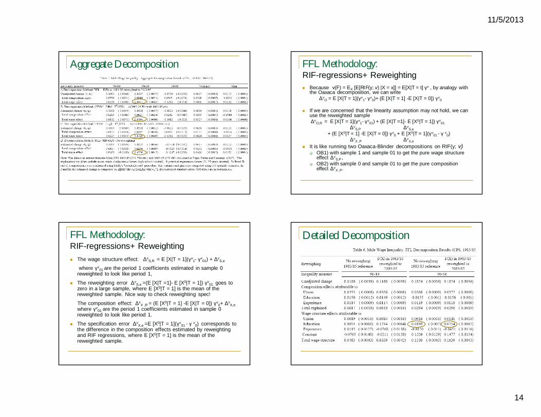
Detailed Decomposition

11/5/2013

15

Detailed Decomposition

Standard errors are obtained by bootstrapping the entire procedure, typical of models involving quantiles, i.e. dependent variable is an estimated variable

Example of bootstrapping procedures, as well as all programs and data for Handbook chapter are downloadable at http://faculty.arts.ubc.ca/nfortin/datahead.html

The “rifreg.ado” routine, that include RIF for variance and Gini, is also available there