Embed Size (px)
Citation preview
Questioni di Economia e Finanza(Occasional Papers)
Non-performing loans and the supply of bank credit: evidence from Italy
by Matteo Accornero, Piergiorgio Alessandri, Luisa Carpinelli and Alberto Maria Sorrentino
Num
ber 374M
arch
201
7

Questioni di Economia e Finanza(Occasional papers)
Number 374 – March 2017
Non-performing loans and the supply of bank credit: evidence from Italy
by Matteo Accornero, Piergiorgio Alessandri, Luisa Carpinelli and Alberto Maria Sorrentino

The series Occasional Papers presents studies and documents on issues pertaining to
the institutional tasks of the Bank of Italy and the Eurosystem. The Occasional Papers appear
alongside the Working Papers series which are specifically aimed at providing original contributions
to economic research.
The Occasional Papers include studies conducted within the Bank of Italy, sometimes
in cooperation with the Eurosystem or other institutions. The views expressed in the studies are those of
the authors and do not involve the responsibility of the institutions to which they belong.
The series is available online at www.bancaditalia.it .
ISSN 1972-6627 (print)ISSN 1972-6643 (online)
Printed by the Printing and Publishing Division of the Bank of Italy

NON-PERFORMING LOANS AND THE SUPPLY OF BANK CREDIT: EVIDENCE FROM ITALY
by Matteo Accornero*, Piergiorgio Alessandri*, Luisa Carpinelli* and Alberto Maria Sorrentino*
Abstract
We employ an extensive dataset on borrower-level loans to study the influence of non-performing loans (NPLs) on the supply of bank credit to nonfinancial firms in Italy between 2008 and 2015. We use time-varying firm fixed effects to control for shifts in demand and changes in borrower characteristics, and we also exploit the supervisory interventions associated with the 2014 Asset Quality Review to identify exogenous variations in the banks’ NPL ratios. We find that banks’ lending behavior is not causally affected by the level of NPL ratios: the negative correlation between NPL ratios and credit growth in our data is mostly generated by changes in firms’ conditions and contractions in their demand for credit. However, the exogenous emergence of new NPLs and the associated increase in provisions can cause a negative adjustment in credit supply.
JEL Classification: E51, E58, G00, G21. Keywords: credit register, credit risk, credit supply, non-performing loans.
Contents
1. Introduction .......................................................................................................................... 5
2. The role of NPLs: transmission mechanisms and existing evidence ................................... 7
3. Our dataset ........................................................................................................................... 9
4. NPL ratios across banks and over time .............................................................................. 11
5. The impact of NPL ratios on credit supply ........................................................................ 13
6. The impact of changes in NPLs on credit supply .............................................................. 16
6.1 A difference-in-difference approach ........................................................................ 17
6.2. An IV approach ........................................................................................................ 18
7. Discussion of the results .................................................................................................... 20
8. Conclusions ........................................................................................................................ 22
References .............................................................................................................................. 23
Figures and tables ................................................................................................................... 25
Appendix: ............................................................................................................................... 38
_______________________________________
* Bank of Italy. DG for Economics, Statistics and Research.

1. Introduction
Does a build-up in non-performing exposures (NPLs) impair banks’ capacity to finance the
real economy? This question ranks high on the list of issues European policy makers have been
grappling with over the past few years. The reasons are clear. Since the onset of the global financial
crisis in 2008, the stocks of NPLs on the balance sheets of European banks have risen substantially;
in Italy NPLs tripled, reaching 18 per cent of total loans in 2015. Besides raising concerns on the
soundness of the banking sector, this phenomenon might trigger a vicious circle where the
contraction in credit supply driven by the level of NPLs lead to lower growth, a slower recovery and
hence a further deterioration in bank balance sheets.
Yet, as of today, formal evidence on the role and importance of bad legacy assets in shaping
banks’ lending policies is hard to come by. Two main issues need to be addressed in this discussion;
one is conceptual, the other methodological. First, the raw correlation between credit quality (either
in stock or flow terms) and credit growth observed in aggregated data can be misleading because
rising NPLs are largely the endogenous product of a prolonged economic stagnation that weakens
both the demand and the supply of credit. Second, there is a good deal of confusion between the
stock and the flow of NPLs as the key factor that could depress lending. The debate has focused to a
great extent on the level of NPL ratios, yet often referring to arguments that are more likely to apply
to variations in those ratios. The implications of higher NPL ratios and increasing NPL ratios are
not necessarily the same, even from a theoretical point of view. High NPL ratios might in principle
exert a permanent effect on banks via a riskier asset side, which could spur the combined influence
on credit of regulatory constraints, market pressures on funding and a risk-taking mechanism. An
increase in NPL ratios presumably produces an effect via profit and loss accounting, inducing banks
to temporarily modify their lending policy while they adjust some quantities, notably provisions, to
restore equilibrium in their balance sheets. In short, assessing whether the stock of NPLs affects
credit supply involves two tasks: one is to disentangle supply and demand, the other one is to
separate the related but distinct mechanisms through which stocks and flows of NPLs might affect
credit.
We address the first issue thanks to the granularity of our unique dataset, where the NPL
ratios of all Italian banks are merged with information on banks’ balance sheets and with data on
borrower-level loans to Italian firms between 2008 and 2015. Since firms typically borrow from
more than one bank at the same time, we can use time-varying firm fixed effects to capture
unobserved changes in borrower characteristics, and test whether banks with different credit quality
behaved in a different way towards the same firm at the same point in time (Jiménez et al., 2014). In
this set up, changes in firms’ profitability, creditworthiness, investment opportunities and demand
5
for funds are separately accounted for, and the significance of the indicator of credit quality – if any
– can be safely interpreted as evidence of supply-side effects.
To examine the impact of the level of NPL ratios, we exploit the variability across banks and
time of the share of non-performing exposures in our large panel of over 500 banks to assess how
this weighs on credit. To separately account for the implications of exogenous variations in NPLs,
we take advantage of the information coming from the Asset Quality Review (AQR), the in-depth
supervisory credit book revision of 130 European banking groups carried out by the European
Central Bank and national supervisory authorities in 2014. If the balance sheet adjustments brought
about by the AQR in December 2014 were (i) not correlated with changes in firms’ conditions in
2015, and (ii) not entirely anticipated by the banks that took part in it, then they can be seen as
exogenous “shocks” and, as such, can help us understand whether fluctuations in NPLs are an
important driver of bank lending.1
We have two main results. First, the level of NPL ratios per se does not influence bank
lending. The negative correlation between NPL ratios and credit growth over the 8 years of analysis
is almost entirely driven by firm-related factors: once these are properly accounted for (in our case,
via time-varying firm fixed effects), a bank’s lending behavior appears to be unrelated to its NPL
ratio. However, consistently with previous literature, we find that other bank-related factors such as
capital ratios and size actively influence credit supply during the period under consideration.
Second, “exogenous” increases in NPLs may have a negative effect on bank lending, similarly to
negative shocks to banks’ capital buffers.
The fact that the NPL ratios did not matter suggests that, in our sample, their movements were
largely driven by cyclical phenomena rather than by bank-specific shocks. In particular, the
correlation in the data must have been caused by a deterioration in economic conditions that acted
simultaneously on banks (causing the increase in NPLs) and firms (leading to a drop in profitability
and a decline in the demand for loans). Of course this result might be specifically related to a period
of prolonged macroeconomic weakness; in more favorable conditions with booming demand for
credit the possibility that high NPL ratios might act as a drag on credit supply cannot be ruled out.
The remainder of the paper is organized as follows. In Section 2 we discuss the economics of
the relation between NPLs and credit supply and we summarize the existing literature on the topic.
In Section 3 we describe our dataset. In Section 4 we present a set of stylized facts on the relation
between NPLs, credit flows and bank funding costs. In Section 5 and 6 we move to a more formal
econometric analysis of, respectively, the level of NPL ratios and NPL variations. The results are
discussed further in Section 7. Section 8 concludes.
1 The logic and limitations of our identification strategy are discussed in detail in Section 6.
6

2. The role of NPLs: transmission mechanisms and existing evidence
In order to examine the relation between NPLs and credit supply, it is useful to make a
distinction between the impact of the level of NPL ratios and the impact of an increase of NPLs.
Simplifying to the core, evaluating how different levels of NPL ratios affect credit supply boils
down to making a sort of comparative statics exercise; gauging the impact of a rise of NPLs is
equivalent to assessing a transition from one state (one with lower NPL) to another (with higher
NPL). Of course, the mechanisms operating in the two scenarios are connected, yet we deem this
distinction particularly useful to clarify the mechanisms at work and we will use it as a guide to our
analysis.
The worse quality of the balance sheet associated to a high level of the stock of NPLs could in
principle affect the supply of credit through three types of channels: a mechanical accounting
mechanism, by which lower credit quality ultimately affects bank capital via risk weights, an
increase in funding costs stemming from heightened market pressures, and a change in the bank’s
risk-taking attitude.
First, high levels of NPLs imply a risky asset side. Given that intermediaries are subject to
prudential regulations on capital, a worsened credit quality translates into higher risk weights on
bank loan portfolios in the calculation of regulatory capital ratios as a measure to cover expected
risk. To cope with increased risk weights and capital absorption banks might decide to reduce the
size of their balance sheet. Furthermore, if the cost of capital becomes permanently higher due to
heightened credit risk, banks might adopt a permanently lower rate of expansion of their asset base.2
A second possibility is that high-NPL banks are forced to scale down their operations by
market pressure rather than deleveraging out of their own will. If a heavier burden of NPLs is taken
as a sign of higher idiosyncratic risk and/or lower managerial abilities, and if this is deemed not to
be fully offset by an adequate coverage ratio, then the bank’s external funding costs should also be
higher. In this case the higher funding costs brought about by higher NPLs can cause a decline in
loan supply.
Finally, NPLs might change banks’ risk attitudes. Thinly capitalized banks are more sensitive
to the “risk taking channel” of monetary policy and more willing to extend credit to weak borrowers
at times of low interest rates.3 Intriguingly, this channel pushes in the opposite direction compared
to those discussed above: in this case high-NPL banks have an incentive to lend more than their
2 Under IRB (internal ratings-based approach), banks must calculate their risk weights on the basis of the losses their realize on non-performing exposures (among other factors); in this case, the managers’ independent response to a rise in NPL might be reinforced by the regulatory pressure due to an increase in the capital absorption of the rest of the loan portfolio. 3 Jiménez et al. (2014).
7
competitors – and possibly more than they should, at overly lax conditions, and/or to the wrong
borrowers – following a ‘gamble for resurrection’ type of logic.4
On the other hand, increases in NPLs might have different implications. An rise of NPLs,
especially if large, unexpected and experienced at times of low profitability, implies a great deal of
adjustment for banks, both automatic and voluntary, to restore balance sheet conditions. Most of
this adjustment operates through the profit and loss account. To keep an appropriate coverage ratio
– and hence protect itself against risk associated to mounting NPLs – a bank must increase loan loss
provisions so to reduce its exposure to the borrowers’ defaults. Higher provisions depress the
bank’s return on assets and, if they are large or prolonged enough, can even cause profits to become
negative, depleting the capital base. In short, the readjustment on the asset side triggered by an
increase in NPLs may have broadly the same implications as a decline in capital, and a depletion of
the capital buffers is known to determine a contraction in credit supply.5
All in all, the lack of a well-defined theoretical framework makes it difficult to fully
characterize the interactions between these mechanisms and the conditions under which each of
them might operate. A higher level of NPL is likely to be associated with permanently higher risk
weights and higher funding costs; its effect on credit depends on whether the bank is able to offset
the contractionary pressures via adequate capitalization and coverage ratios. Since it relates to the
overall solvency of the bank, the risk appetite channel might also depend on the outstanding stock
of NPLs, particularly if the informational asymmetry between managers and external stakeholders
are pronounced and insiders have much better information on the actual quality of the assets. On the
other hand, an increase in NPL triggers mechanisms that rely on frictions that banks ought to be
able to mitigate in the longer term, when they have the possibility to raise capital or adjust
provisions without squeezing their profit margins too heavily.
The literature has thus far focused on the drivers rather than the implications of NPLs. These
have been found to depend both on bank characteristics and on the macroeconomic performance of
the economies where the banks operate.6 The relevance of macroeconomic dynamics highlights the
key endogeneity issue that undermines any attempt to identify a causal impact of NPLs on credit
supply: NPLs rise in countries and periods where economic activity stagnates and, consequently,
creditworthiness is deteriorated and the demand for credit also tends to be weak. This means that a
negative correlation between NPLs and credit volumes, in and by itself, means very little. The role
of bank-specific factors, on the other hand, corroborates the idea that NPLs might also act as a 4 See e.g. Krugman (1998). 5 See e.g. Froot and Stein (1998), Van den Heuvel (2008), Aiyar et al. (2014). Capital buffers also matter for the transmission of monetary policy (Gambacorta and Mistrulli, 2004). For the role of capital during crises, see Beltratti and Stultz (2012), Berger and Bouwman (2013), Dagher et al. (2014). 6 Bofondi and Ropele (2011), Louzis et al., (2012), Klein (2013), Messai and Jouini (2013).
8
signal on the (idiosyncratic) weakness or misbehavior of the underlying banks. Increases in NPLs
are indeed often anticipated by credit expansions and a loosening of lending standards.7 They are
also associated with prior reductions in banks’ overall cost efficiency, suggesting that the two
phenomena (high costs and high NPLs) might be symptoms of a common underlying problem, such
as poor managerial practices.8 As of today, however, little is known as to whether and how these
factors exert any influence on banks’ lending strategies.
Kaminsky and Reinhart (1999) note that high NPLs are often associated with the outbreak of
banking crises but both can be the result of macroeconomic forces that weaken simultaneously the
banking sector and the real economy, such as strong exchange rate appreciations. Balgova et al.
(2016) study the relation between output growth and changes in NPL stocks using aggregate data on
a panel of 100 countries between 1997 and 2014, finding that countries that actively reduced their
NPLs typically experienced higher growth rates. Bending et al. (2014) estimate dynamics
regressions using bank-level data for a sample of intermediaries from 16 European countries
(excluding Italy) and document that both NPL ratios and changes in NPLs are negatively correlated
with net growth in corporate and commercial loans in the following year. Cucinelli (2015) obtains a
similar result for Italy, arguing that both NPLs and the loan-loss provision ratio (two similar proxies
of the credit quality of the bank’s portfolio) have a negative impact on the supply of bank loans. A
common denominator on these works is the high level of aggregation of the data. The evidence
points to a strong negative correlation between NPLs and credit; however, endogeneity problems
are pervasive, and imply that moving from a statistical to a causal statement on the basis of country-
or bank-level observations is fairly problematic. Against this backdrop, our main contributions to
the debate are to (i) discriminate more explicitly between stocks and flows of NPLs, and (ii) exploit
a loan-level dataset where identification is stronger and causality can be established with a higher
degree of confidence.
3. Our dataset
Our analysis is based on an extensive dataset at the bank-firm level. For every firm we gather
information on credit obtained by any bank operating in Italy.9 For every bank, in turn, we recover a
large set of balance sheet indicators, including the NPL ratios. We rely on two main sources.
7 Keeton (1999), Jiménez and Saurina (2006). 8 Berger and De Young (1997). 9 We consider banking groups and individual banks for those not belonging to a group.
9
For bank-firm credit relationships we use information on outstanding loan amounts from the
Italian Credit Register (henceforth CR), over the period from 2008 to 2015. The CR records various
end-of-year information on all loans exceeding 30,000 euros.10 We focus on all non-financial firms,
including very small firms, such as sole proprietorships. Data on credit quantity consists of both
granted and drawn credit; as dependent variable we focus on granted credit, as this is more
responsive to supply dynamics. Loans are made of three different categories of credit: revolving
credit lines, term loans and loans backed by accounts receivable.
Our firm-level dataset includes overall 500 banks and more than 2 million borrowers, totaling
more than 4 million bank-firm relationships. In order to control for unobservable heterogeneity
through firm-time fixed effects, in our regressions we only include firms borrowing from at least
two banks. This still leaves more than 2 million bank-firm relationships, given that multiple lending
is particularly common in Italy across a large set of firms (Detragiache et al. 2000, Gobbi and Sette
2014), and therefore is not too restrictive of a condition. For computational reasons, when running
our regressions, we select a random sample of about 20 per cent of this universe.
Table 1 displays some basic statistics on our data. The first panel shows the average changes
in log credit granted over time, corresponding to the left-hand side variable that will be used in our
regressions. Credit granted to all firms decreased on average in all the years under analysis. The
statistics are reported for the whole of the banking sector and for some categories of intermediaries.
In particular we look at banks that underwent the Comprehensive Assessment of 2014 (AQR banks)
versus the remaining ones, and we also isolate mutual banks.11 This first distinction, as we will see
later, is particularly useful to try to assess the impact of exogenous variations of NPLs on credit
supply.12
We use bank-level information on a consolidated basis from the Supervisory and Statistical
Reports submitted by the intermediaries to the Bank of Italy. We gather information from both
balance sheet and profit and loss accounts to build some sensible indicators of banks’ structure and
health. The main variables that we consider are total assets, as a proxy of size, Tier 1 Ratio to
capture capitalization, Return on Equity for profitability, provisions over operating profit to assess
10 The threshold was reduced from 75,000 to 30,000 euros in 2009. In the analysis in which we include 2008 we restrict our sample to include only loans above the initial threshold of 75,000. For analysis restricted to post-2009 periods, we keep the threshold at 30,000 11 Mutual banks are characterized by a different business model with respect to other banks; they are local and not-for-profit cooperatives. Even if the recent legislative reform had the aim to stimulate these banks to be more integrated through the institution of a cooperative banking group, in the period under analysis these banks acted as a very different player. 12 In the appendix other data are reported as derived from the CR, which show the patterns of three very relevant features of bank-firm relationships. They will be used in our causal analysis to take into account the specific characteristics of the matching between borrowers and lenders.
10
the relevance of the yearly flows of provisions on operating margins and finally the cost to income
ratio as a measure of efficiency.
Table 2 shows how these variables changed over the period 2008-2015, for the aggregate of
the banking sector as well as across the sample split we already used for Table 1. Clearly, average
NPL ratios went up dramatically and the phenomenon was widespread across bank types. In
particular, the NPL ratio almost tripled since the beginning of 2008 for AQR banks and more than
tripled for other banks, including mutual banks. As a consequence, the impact of provisions over
operating profit grew largely between 2008 and 2014. In particular, there was a spike in 2013 and
2014, associated with the aforementioned Asset Quality Review. The flip side of the coin was that
profitability, which had declined since the beginning of the period analysed, turned negative in
2011, and again in 2013 driven by AQR banks that had been already recording losses since 2013; at
the same time, coverage ratios increased, reaching an average of 45 per cent. This was not
associated with a significant deleveraging process, given the continuous increase in capital.
Capitalization indeed grew throughout the 8-year period. For smaller banks, it almost reached 17
per cent; for larger banks (such as the AQR ones), after a steady increase, tier 1 ratio stood at over
12 per cent by the end of 2015.
4. NPL ratios across banks and over time
We start by exploiting bank-level data to illustrate how the relation between NPLs and credit
evolved in Italy over the last decade. Figure 1 documents that the aggregate NPL ratio has been
rising consistently over time. The aggregate ratio of NPLs over total credit was just around 6 per
cent at the outbreak of the Lehman crisis and it grew constantly reaching almost 20 per cent over
the following seven years. Credit growth to the Italian economy was negative for more than half of
the period under examination (Panel A). Panel B confirms that the phenomenon is particularly
pronounced for loans to firms.
To provide more informative qualitative evidence we also study heterogeneity across banks.
In particular, we examine the correlation between the banks’ NPL ratios measured at three specific,
important dates and their subsequent performance in terms of lending and profitability. The first
date we pick is the end of 2008: this provides a picture of the system in the immediate aftermath of
the Lehman default, at a time when Italian banks had not yet been affected by the global financial
crisis. The second snapshot is taken at the end of 2010, before Italy was hit by sovereign shocks that
caused further financial market distress (Bofondi et al. 2017) and the second prolonged recession
11
within less than ten years. The third date is December 2015: by that time the impact of the global
and sovereign shocks had fully materialized.
In the scatterplot of Figure 2 banks’ credit growth rates between 2008 and 2015 (vertical
axis) are plotted against their initial NPL ratios (horizontal axis). The correlation is very low. If one
separates the two sub-periods 2008-2010 and 2010-2015 (Figure 3), it becomes clear that in the first
two years after the Lehman crisis the correlation between credit quality and credit growth was
extremely weak and, if anything, positive rather than negative (green line). On the contrary, banks
that had higher NPL ratios as of December 2010 do seem to have lent less in the following years
(red line). The link remains however very tenuous leaving leeway to further investigations aimed at
finding possible answers to our research question.
The relationship between initial NPLs and future credit quality does not provide a clear
picture. In Figure 4 the banks are sorted on the horizontal axis based on their pre-Lehman NPL
ratios and the scatterplots show how these changed between 2008 and 2015. The initial ratios,
displayed in red, range from zero to just below 35 per cent. The distribution is roughly unchanged at
the end of 2010 (green dots). By the end of 2015 (blue dots) the increase in NPLs is more
pronounced and, more importantly, the initial ranking across banks is entirely lost: many of the
banks whose initial NPLs were below 10 per cent, for instance, appear to be in the same situation as
those that started with NPLs of 20 per cent or higher. This confirms that the cyclical conditions of
the Italian economy – a systemic risk factor common to all banks – were an important driver of the
NPLs.
To check whether banks with high NPL ratios share other common balance sheet
characteristics we examine next the relation between NPL ratios and some basic balance-sheet
indicators. In Figures 5-7 we plot the correlation between NPL ratios and, respectively, the log of
total assets, capital ratios and the cost to income ratio, focusing again on the three pivotal dates of
end-2008, end-2010 and end-2015. Figure 5 shows that up to 2010 higher NPLs were concentrated
among small banks, while by 2015 they had largely increased for all banks regardless of their size.
This widespread growth is consistent with figure 4 and is another sign of the emergence of
aggregate drivers of the NPLs linked to weak macroeconomic conditions. Figure 6 shows that the
correlation between NPLs and capital is fairly weak and changed sign over time, with a higher
concentration of NPLs in less capitalized banks at the end of our sample. Interestingly operating
costs seemed to be positively correlated with credit quality at times of low NPLs, as shown in
Figure 7. Although this correlation might be caused by a number of factors, one possibility is that a
higher presence of bank personnel and/or higher investments in IT might make intermediaries more
capable of screening and monitoring their clientele. In 2015 cost to income ratios had become much
12

less heterogeneous across banks with different credit quality, perhaps because the deep recession
had again largely wiped off longitudinal differences in the relationship between banks’
characteristics and NPL ratios.
The descriptive evidence suggests three broad remarks. First, balance sheet conditions
deteriorated rapidly for most banks, with soaring NPL ratios that also affected profitability. Second,
mechanisms of a prudential nature, both regulatory and self-enforced, were activated by the banks,
such as raising the coverage ratio and strengthening the capital base, with the aim of increasing
resilience, even at the cost of weakening current profits. Third, as we can argue from the figures,
banks with high NPL ratios do not share common balance sheet characteristics. Therefore the
accumulation of legacy assets across the population of banks must have been largely affected by
aggregate macroeconomic conditions. These also act on the demand side of the credit market.
Hence, this conclusion is also a reminder of the difficulty of identifying the supply-side effects of
NPLs.
5. The impact of NPL ratios on credit supply
As we said above, correlations can be informative, but only up to a point. The co-movements
between banks’ NPL ratios and their contemporaneous or future economic performance, including
their lending behavior, can be generated by a range of mechanisms many of which do not imply a
causal role for the quality of the banks’ portfolios. In order to move from correlation to causation
we use regression analysis. We estimate a credit supply equation where NPLs feature as a potential
driver of banks’ lending strategies and firm-time fixed effects are used to control for changes in
observed and unobserved borrower characteristics and for changes in demand. The presence of
time-varying effects at the firm level is made possible by the combination of firm-level data and
multiple lending relations between banks and firms and it clearly sets our analysis apart from
previous studies (see Section 2).13 We estimate the following benchmark regression:
∆ = + + + ∑ + . (1)
The dependent variable is the yearly (log) growth in credit granted by bank i to firm j at time
t. The advantage of using a borrower-level dataset that includes multiple lending relations is that a
time-varying borrower-specific effect αjt can be included among the regressors to control for shifts
13 The strategy was pioneered by Khwaja and Mian (2008).
13
in borrowers’ characteristics, including demand. Intuitively, as long as the demand-side shocks that
affect firm j (including for instance a drop in sales, or lack of investment opportunities) influence all
of its lending relations in the same way, the fixed effect αjt guarantees that their influence is
removed from the data and that the remaining regressors in equation (1) capture exclusively supply-
side factors. The presence of αjt is thus essentially what allows us to interpret the rest of the
equation as a model of the supply of credit. The key regressor is of course the bank-specific NPL
ratio (NPLit-1): if this ratio matters, banks with high NPLs should have lent less to firm j for any
given level of borrower characteristics, leading to γ<0. The regression also includes bank fixed
effects (αi) and various bank-level controls (Xit-1). Our measure of NPL ratio is net of the stock of
provisions.14
To get a better picture of the mechanism of interest, we start off with a naïve version of
equation (1) that does not include bank and firm controls and we then build it up by gradually
adding more information. The results are summarized in Table 3. The coefficient obtained from the
simple, univariate OLS regression in column 1 is positive but not significant. By introducing firm
fixed effects (column 2) we move to a ‘within firm’ type of analysis. This delivers a negative and
significant coefficient which is in line with what one might expect looking at patterns in the data:
for a given firm, high NPLs in the balance sheet of the lender are associated to a decline in credit
which is at least consistent with NPLs discouraging bank lending. The negative coefficient in
column 2 implies that the correlation between NPL ratios and credit is not entirely explained by
fixed firm characteristics: in other words, it rules out the possibility that firms that are altogether
“bad” (on account for instance of low productivity or poor management) are entirely responsible for
the link between high NPLs and declining credit flows in the data. A number of possible
interpretations remain open though. In particular, this specification cannot discriminate between (i)
a genuine supply-side effect of the NPL ratios and (ii) a plain correlation between NPLs and credit
caused by shocks that affect both banks and firms – such as those linked to the macroeconomic
cycle.
We introduce firm-time fixed effects in column 3, and keep them in all subsequent
specifications. Even without any additional control variable, the presence of these dummies renders
the NPL ratio statistically insignificant. This means that the behavior of two hypothetical banks in
our sample towards a common borrower j at any time t was not influenced by their NPL ratios. We
emphasize again that it is the presence of firm-level time-varying fixed effects (and hence of a
14 We could otherwise include the indicators of Gross NPL ratio and coverage ratio as two distinct regressors, and account separately for the impact of each. Yet we choose the more parsimonious version with just Net NPLs, as we deem that it incorporates the combined effect of credit quality and provisions. Results are robust to jointly introducing gross NPL ratios and coverage ratios.
14
bank-borrower level dataset) that makes it possible to draw this conclusion. This result is crucial in
answering our first question. The lack of significance of the regressor in column 3 implies that the
correlation between NPL ratios and credit growth in the data is driven by variations in borrower
characteristics. These are likely to include changes in firms’ riskiness, profitability and investment
opportunities, all of which largely deteriorated over our estimation sample. Changes in demand
could play an important role too. The demand for credit generally weakens in recessions, when
firms have fewer investment opportunities and are more uncertain about their future. Furthermore,
Alfaro et al. (2016) show that opaque and financially-constrained firms have a precautionary reason
to reduce their debt in ‘bad times’ (i.e. when volatility is high). This means that credit demand does
not change in the same way for all firms over the cycle. The number of financially-constrained
firms increases in bad times. If these firms demand less credit for precautionary reasons, then the
correlation between rising NPL and falling credit in column 2 might also be driven by demand
factors, which are instead removed by the firm-time fixed effects included in column 3.
The remainder of table 3 shows that the conclusion is confirmed if relationship-related
controls are added to the regression, i.e. if we account for some observable characteristics of the
bank-firm relationships (Column 4). Interestingly, results hold also when taking into consideration
bank-level time invariant heterogeneity, that is, when we plug also bank fixed effects (Column 5).
This is a particularly important specification, in that it controls for the different structural features of
banks, such as business models, that might have played a role in affecting bank credit supply.
Column 6 presents an even more demanding specification where the usual firm-time effects are
combined with bank-firm fixed effects that allow for possible unobserved non-random matching
between banks and firms. The conclusion is unchanged, as NPLs ratios are again irrelevant in
explaining change in granted credit.
Our descriptive statistics show that 2008-2015 was a period of rapidly changing (and mostly
deteriorating) balance sheets, so it is also important to examine the relevance of other balance sheet
indicators whose concurrent evolution accompanied the rise in NPL ratios. In Table 4 we expand
the specification of Table 3 to introduce observable bank characteristics such as size, capital ratio
and ROE. We repeat the regression with time-invariant firm fixed effects (column 1, like column 2
of Table 3), with firm-time fixed effects (column 2, like column 3 of Table 3), and with bank fixed
effects and relationship controls, to thoroughly account for structural and cyclical bank
heterogeneity and bank-firm non-random matching. The results show that also when including other
time-varying bank features, the NPL ratio remains insignificant (column 3, like column 5 of Table
3). Unlike the NPL ratio, bank capital is positive and significant in all three specifications. Finally,
bank size enters negatively if bank fixed effects are included, suggesting that banks that have grown
15
‘too big’ (relative to their average size over the period, which is captured by the fixed effect) are
relatively less willing to extend new credit. Notably, regressions without the bank fixed effects
show how mutual banks’ credit growth was consistently higher relative to other banks.
Before moving to the AQR analysis we briefly discuss an alternative version of table 3 where
the NPL ratio is replaced by the flow of new bad loans over outstanding loans (New Bad Loan
Rate), again lagged relative to the dependent variable. This flow variable measures the variation in
the lowest-quality segment of the banks’ NPLs and, as such, should capture some of the exogenous
shocks that hit banks’ balance sheets in our sample period. The results are reported in Table 5. The
coefficients are qualitatively similar to those obtained in the specifications based on the NPL ratios,
but the bad loan rate achieves statistical significance, albeit weak, even in some of the regressions
that include firm-time effects (see column 4). This is a first indication that NPL shocks might matter
even if the NPL ratio per se does not. However, this regressor may still be affected by an
endogeneity problem. In the next section we try to exploit the Asset Quality Review to get around
this problem.
6. The impact of changes in NPLs on credit supply Even if high NPL ratios do not discourage banks from lending, an exogenous variation in
these ratios may push them to change their lending policies. In this case NPLs do not constitute a
drag for the credit market but their fluctuations can cause a temporary contraction in the supply of
credit. To examine this possibility we adopt an ‘event study’ approach and study lending dynamics
around the 2014 Asset Quality Review (AQR) carried out by the European Central Bank.
The AQR was part of the Comprehensive Assessment, a year-long examination of the
resilience and positions of the 130 largest banks the euro area that the ECB undertook, together with
national supervisors, in preparation of the launch of the Single Supervisory Mechanism (SSM). The
AQR consisted in a check of the quality of the assets held at the end of 2013, based on a set of
common definitions. Much of its focus laid in the analysis of the loan book, and it basically verified
two aspects on a sample of loans selected from the riskiest portfolios: (i) the accuracy of loans’
classification in the performing and non-performing categories; (ii) the adequacy of the related
provisions, taking account of the valuations of the collateral covering the exposures. The second
step of the Comprehensive Assessment was to quantify the capital strengthening measures to be
taken, based on a stress test conducted with reference to a baseline and an adverse macroeconomic
scenario. Fifteen Italian banks took part in the comprehensive assessment; of these, 13 now fall
directly within the perimeter of the SSM.
16
If the balance sheet revisions associated to the AQR were at least in part (i) independent of the
business cycle conditions faced by the bank borrowers in the subsequent year and (ii) unanticipated
by the banks, then they can be interpreted as exogenous variations in the quality of the balance
sheets and exploited to understand how (if at all) banks adjusted their lending in response to them.15
We exploit this idea in two ways.
6.1 A difference-in-difference approach
First, we consider the whole set of Italian banks and compare the lending behavior of AQR
banks to that of non-AQR banks before and after the exercise, within a difference-in-difference type
specification.16 As mentioned, the AQR led to an increase in provisions and requirements across the
participating banks. Furthermore, the fact of being included in the review meant that these banks
faced at least a non-negligible risk of having to deal with a (supervisor-driven) downward revision
in the quality of their portfolios. This might have been a good enough reason to lend more
conservatively. Hence, the AQR might have induced a systematic downward shift in credit supply
for banks that were subjected to the review relative to those that were not.17 We examine this
possibility by testing whether the banks that received the “AQR treatment” displayed a different
lending behavior in the aftermath of the review compared to those that did not. Defining adequate
pre- and post-treatment time windows in this setup is far from trivial. We consider 2012-2013 as
the pre-treatment period and 2014-2015 as the post-treatment period. The AQR was announced on
October 23rd 2013, and conducted throughout 2014 based on bank-balance sheet results of end-
2013. Nevertheless, since (i) the review appeared in the media well before being its official
announcement, and (ii) banks tend to smooth out their balance sheet adjustments if possible,
focusing on too narrow a window of a few months around the end of 2014 would be misleading.
The results are reported in Table 6. Our dependent variable is the log change in credit
growth. Columns 1 and 2 show the simplest diff-in-diff specification, comparing the difference in
growth over the two periods between the two subsamples of banks via a bank dummy (AQR bank)
15 Both assumptions are rather demanding. Supervisors might have taken into account the characteristics of loan portfolios following 2013, and the nature, scope and broad objective of the AQR were obviously not a surprise for the banks in any way. However, while banks used a variety of internal models, the AQR was conducted based on a shared and unique framework. This implied that supervisors had limited margins for adopting different approaches towards different banks and based most of their assessments on end 2013 balance-sheets. Furthermore, the complexity of the process and the discrepancies among models were such that banks were unlikely to be able to accurately predict the outcome of the review. The identification strategy we discuss below hinges on the presumption that there were non-negligible differences between what the banks expected and what they observed when the process ended in December 2014. 16 The analysis is again conducted using matched bank-firm relations and firm fixed effects on the same dataset that was employed for the analysis of Tables 3-5. 17 Moral suasion and competitive pressures might have blunted the actual difference between being inside and outside the AQR list to some extent, but it is unlikely that they made it entirely irrelevant.
17
and a time dummy (post AQR). The positive coefficient in column 1 reveals that lending was on
average higher for AQR banks and this differential pattern continued after the supervisory exercise,
even when we take into account systematic bank differences by including bank fixed effects
(column 2). Column 3 and 4 allow to gauge whether heterogeneity in NPL ratios induced banks to
adjust their credit supply differently after the review took place. Interestingly, AQR banks still
appear to have lent at higher rates on average (column 3), but not more intensely in the AQR period,
as the interaction between the time and the bank dummy shows (columns 3 and 4). NPLs per se do
not weaken lending growth; in fact, NPL ratios have a puzzling positive coefficient. Nevertheless,
the negative interaction between NPL ratios and AQR dummy shows that AQR banks that had a
higher share of non-performing exposures lent on average relatively less, supporting the case of a
differentiated behavior across AQR banks based on their initial credit quality. As shown by the
triple interaction in column 4, after the revisions induced by the AQR, though, the impact of NPL
ratios within AQR banks seems mitigated. A possible interpretation for this is the improvement in
transparency and confidence yielded by the review; however many other factors, including a
relative improvement in macroeconomic conditions, could have played a role too.
The diff-in-diff specification suggests that the relation between NPL ratios and credit is not
clear-cut; in most cases the share of non-performing loans becomes insignificant once demand and
bank-level characteristics are properly accounted for, in line with the results in Section 5. At the
same time Table 6 suggests that the AQR subsample contains a great deal of heterogeneity, which
is precisely what we exploit in the next subsection.
6.2 An IV approach
The second step in our exploration of the AQR aims at identifying the impact on credit supply
of an exogenous variation in NPLs. The focus of the analysis therefore shifts to two measures of
changes in credit quality: the flow of provisions over operating profits (Provisions/Operating
Profits) and the flow of new NPLs over total outstanding loans (NewDefault rate). Since we are
after the effect of a variation in credit quality, these flow measures are more informative than the
underlying NPL ratios.
The revisions in banks’ balance sheets related to the AQR exercise provide a valuable
instrument for the change in credit quality recorded in 2014-15. For the 15 Italian banking groups
that were subjected to the AQR we use both reclassifications from performing to non-performing
portfolios and additional provisions set aside as a result of the review. These figures allow us to
18
build our two instruments: two measures of (AQR-related) changes in provisions and in NPL
ratios.18 We use the two following specifications:
∆ = + ⁄ + +
(2) ∆ = + + + The dependent variable is the log change in credit granted by bank i to borrower j between
2013 and 2014 and between 2014 and 2015. The key regressors are, alternatively, the flow of
provisions over operating profits that took place in 2014-15 (Provisions/Operating Profits), and the
flow of new NPL over total outstanding loans (NewDefault rate). Both indicators measure by how
much credit quality deteriorated in the period under analysis in banks’ balance sheets. Exploiting
our loan-level dataset, we again introduce a set of firm fixed effects (αj) that capture the overall
change in credit for each borrower over the period of interest. These are effectively the static
version of the firm-time fixed effects used in the regressions of Section 5. As in the previous case,
they are extremely important for identification because they allow us to focus on the differences
between banks that were lending to the same firm. The lagged net NPL ratio is included in the
controls (X) in all specifications.
We analyze Provisions/Operating Profits first. In order to focus on its exogenous variation we
instrument the regressor using alternatively two of the official outcomes of the AQR, namely (i)
provisions, expressed in basis points or as share of total assets, and (ii) variations in NPL ratios
associated with the reclassifications of loans to non-performing categories. The results are reported
in Table 7. The regressions are estimated both with and without bank characteristics and include the
usual set of relationship controls. The coefficient of interest is negative and significant in four
specifications out of six (see columns 3 to 6). This suggests that the negative adjustments that banks
had to make after the AQR did have a negative impact on lending.
In Table 8 we replicate the analysis using the New Default rate as a regressor instead of the
ratio of provisions to profits and instrumenting it with the variations in provisions and the variations
in NPL ratios brought about by the supervisory revision. As in the previous case, the exogenous
18 The validity of our instruments is confirmed by the first stage of the 2SLS estimation. All three instruments (AQR provisions in basis points, AQR provisions over total assets, and AQR-related NPL ratio change) appear to be well correlated with two endogenous variables (Provisions over Operating profits and New Default rate). The F test of excluded instruments is always way higher than threshold levels for not having weak instruments (Angrist and Pischke, 2009).
19

variation in default rates – as captured by the IV strategy – has a broad negative impact on credit
growth in four out of six specifications.
7. Discussion of the results The instrumental variable estimates discussed in Subsection 6.2 suggest that exogenous
shocks to the banks NPL ratios can indeed have a negative impact on credit supply. The opposite
conclusion would be very surprising. If and when they occur in a genuine ceteris paribus setup –
i.e. holding fixed banks’ coverage and capital ratios, their lending opportunities, etc. – NPL shocks
indeed are intuitively similar to other negative “exogenous” shocks that impair capitalization,
liquidity or profitability. These shocks have been documented in the literature to be relevant for
credit supply, and assessing their specific repercussions is beyond the specific focus of our paper19;
our analysis shows that exogenous shocks to credit quality go in the same direction. At the same
time, the regressions with firm-time fixed effects presented in Section 5.1 show that the link
between NPL ratios and credit growth in the data becomes very tenuous (in fact non-existent) if the
specification is rich enough to control properly for changes in observed and unobserved borrower
conditions. This finding is a signal that a decline in firms’ profitability, investment opportunities
and demand for credit might be the key common factors behind both the rise in NPLs and the drop
in credit flows. Demand might have played an important role too. At times of high economic
uncertainty, firms are known to invest less, which causes a decrease in their need for external
funding. Furthermore, firms that are exposed to the risk of losing access to credit markets
voluntarily engage in deleveraging with the aim of enhancing their resilience to adverse
idiosyncratic shocks.20
Taken together, this evidence suggests that, although important in principle, exogenous NPL
shocks must have played in practice a relatively minor role in Italy over the last decade. If the NPL
ratios had been fluctuating under the influence of exogenous shocks to the banks’ balance sheets (as
those associated to the AQR), then based on the IV results we would expect them to be a significant
driver of bank lending in our full-sample regressions. Clearly, that is not the case. A corollary of
this conclusion is that the NPL ratio in and of itself is unlikely to constitute a problem. Banks are
19 See e.g. Peek and Rosengren (2000), Khwaja and Mian (2008), Peydrò (2010) and Mora and Logan (2012). Although we do not identify specific shocks to capital or profitability, we use these balance sheet indicators as bank-level controls and find that the Tier 1 ratio has a positive effect on credit even after controlling for time-varying firm characteristics (see table 4). This confirms that capital is a relevant driver of bank lending in our sample too, as predicted by this strand of research. 20 Alfaro et al. (2016).
20

equipped to deal with non-performing exposures, and in a static situation (i.e. barring shocks) the
ratio would not snuff credit out irrespective of its level.
Finally, our diff-in-diff analysis of the AQR can be read as a way of checking what was the
relevance of genuine NPL shocks, or more generally the relative role of supply and demand factors,
in the delicate transition faced by the Italian economy between 2012 and 2014. Our results show
that, despite the causal effects revealed by the IV estimates, the AQR did not, all in all, decrease the
supply of bank credit. The negative impact of the review on the key balance sheet items, including
non-performing exposures, must have been quantitatively limited and more than compensated by
the positive impact of higher confidence and transparency.
We focus on the intensive margin of credit. NPLs might of course also influence credit supply
along other dimensions, for instance making loans more expensive or causing rationing problems.
Although it seems unlikely that these would vary leaving credit quantities unchanged, a more
thorough investigation of these possibilities would certainly be a worthwhile extension of
our work.
Where does this leave the debate on NPLs? If (i) the correlation between NPL ratios and
credit flows is largely endogenous, and (ii) the ratios only really ‘matter’ when they fluctuate for
exogenous reasons, it follows that any statement on whether or not NPLs constitute a problem
should be made conditional on a clear identification strategy and a reliable estimate of the nature
and size of the shocks faced by banks. Our empirical results do not extend of course to other
economies, nor necessarily to different historical episodes, but they clearly illustrate the crucial role
of identification in making causal statements on the relation between NPLs and credit dynamics
21
8. Conclusions
The steep increase in non-performing bank loans (NPLs) that took place after the financial
crises of 2008-2011 has brought the problem of ‘legacy assets’ to the center of the European policy
debate. If a decline in the quality of the loans discourages bank lending, the rise in NPLs observed
since 2008 might have played an important role in depriving European economies of much-needed
credit, making the recovery from the crisis harder than elsewhere. The case of Italy is an interesting
one to test this possibility: between 2008 and 2015 the aggregate NPL ratio of Italian banks
doubled, credit shrunk, and the country – where the structural relations between banks and firms are
notoriously strong – experienced two distinct recessions.
To investigate the linkage between NPLs and the supply of bank credit, we construct a rich
dataset that includes the universe of Italian banks and the evolution of their lending relations with
2.5 million borrowers over the last 8 years. The availability of loan-level information from the
Italian Credit Register allows us to control thoroughly for changes in the demand for credit: in
particular, we can zoom in on firms that were borrowing from more than one bank at once and
check whether they systematically obtained less funds from lenders that were burdened by a higher
NPL ratio. We also exploit for identification purposes the Asset Quality Review (AQR) carried out
by the European Central Bank in close cooperation with supervisory authorities in 2014.
Supervisors forced a number of adjustments to bank balance sheets which, being out of the control
of the banks, can be seen as an “exogenous” source of variation in NPLs.
We find that, although exogenous shocks to NPLs can indeed cause a decline in credit supply,
the correlation between NPLs and credit in our data is almost entirely driven by demand-side
effects. Once these are accounted for, NPL ratios have no discernible influence on banks’ lending
strategies. Our analysis also suggests that the overall impact of the AQR on bank lending was
positive rather than negative. At the margin, the revisions in write-downs and NPLs imposed by the
supervisors were bad news for both banks and borrowers; but bank lending rose in aggregate terms
after 2014, possibly on account of the decrease in uncertainty generated by the evaluation exercise.
In the current conjuncture improving resilience and rebuilding confidence in the banking
sector remains a critical policy objective, both in Italy and elsewhere. Addressing legacy assets is an
important part of this process. However, our work suggests that NPLs are an easy but unlikely
culprit for the weak credit flows observed in the past years, and that their role in shaping bank
behavior might be easily overestimated. Our results also suggest that forcing banks to liquidate
NPLs may not be the best option to kick-start credit. It might even be counterproductive; if the
liquidation of the NPLs generates losses that are large enough to reduce the banks’ capital ratios,
then, given that NPLs do not seem to matter while capital certainly does, the net impact of the sale
on credit supply might be negative rather than positive.
22
References
Alfaro, I., N. Bloom, X. Lin, 2016, The Finance-Uncertainty Multiplier, Stanford University
mimeo. Aiyar, S., C. W. Calomiris, J. Hooley, Y. Korniyenko, T. Wieladek, 2014, The international
transmission of bank capital requirements: Evidence from the UK, Journal of Financial Economics, 113, 3, 368-382.
Angrist, J. and J. Pischke, 2009, Mostly Harmless Econometrics: An Empiricist's Companion,
Princeton University Press. Balgova, M., M. Nies, A. Plekhanov, 2016, The economic impact of reducing non-performing
loans, European Bank for Reconstruction and Development Working Paper, 193. Beltratti, A., and R.M. Stulz, 2012, The credit crisis around the globe: why did some banks perform
better?, Journal of Financial Economics, 105, 1–17. Bending, T., M. Berndt, F. Betz, P. Brutscher, O. Nelvin, D. Revoltella, T. Slacik, M. Wolski, 2014,
Unlocking lending in Europe, European Investment Bank. Berger, A.N., and C.H.S. Bouwman, 2013, How does capital affect bank performance during
financial crises?, Journal of Financial Economics, 109, 1, 146-176. Berger, A.N., and R. De Young, 1997, Problem loans and cost efficiency in commercial banks,
Journal of Banking and Finance, 21, 849–870. Bofondi, M., L. Carpinelli, E. Sette, 2017, Credit Supply during a Sovereign Debt Crisis, Journal of
European Economic Association (forthcoming). Bofondi, M. and T. Ropele, 2011, Macroeconomic determinants of bad loans: evidence from Italian
banks, Bank of Italy Occasional Paper Series, 89. Cucinelli, D., 2015, The Impact of Non-performing Loans on Bank Lending Behavior: Evidence
from the Italian Banking Sector, Eurasian Journal of Business and Economics, 8, 16, 59-71. Dagher, J., G. Dell’Ariccia, L. Laeven, L. Ratnovski, H. Tong, 2014, Benefits and Costs of Bank
Capital, IMF Staff Discussion Note, 16/04. Detragiache, E., P. Garella L. Guiso, 2000, Multiple versus Single Banking Relationships: Theory
and Evidence, Journal of Finance, 55, 1133-1161. Froot, K.A. and J. Stein, 1998, Risk management, capital budgeting, and capital structure policy for
financial institutions: An integrated approach, Journal of Financial Economics, 47, 1, 55–82.
23
Gambacorta, L., and P. E. Mistrulli, 2004, Does bank capital affect lending behavior?, Journal of
financial intermediation, 13, 436-457.
Gobbi, G. and E. Sette, 2014, Do Firms Benefit from Concentrating their Borrowing? Evidence from the Great Recession, Review of Finance, 18, 2, 527-560.
Jiménez, G. and J. Saurina, 2006, Credit cycles, credit risk and prudential regulation, International Journal of Central Banking, 2, 65-98.
Jiménez, G., S. Ongena, J.L. Peydró, J. Saurina, 2014, Hazardous Times for Monetary Policy: What Do Twenty-Three Million Bank Loans Say About the Effects of Monetary Policy on Credit Risk-Taking?, Econometrica, 82, 463-505.
Kaminsky, G.L. and C.M. Reinhart, 1999, The Twin Crises: The Causes of Banking and Balance-of-Payments Problems, The American Economic Review, 89, 3, 473-500.
Keeton, W. R., 1999, Does faster loan growth lead to higher loan losses?, Federal Reserve Bank of Kansas City Economic Review, 84, 57-75.
Khwaja, A. I. and A. Mian, 2008, Tracing the impact of bank liquidity shocks: evidence from emerging market, American Economic Review, 98, 4, 1413-1441.
Klein, N., 2013, Non-Performing Loans in CESEE: Determinants and Impact on Macroeconomic Performance, International Monetary Fund Working Paper, 13/72.
Krugman, P., 1998, It's Baaack: Japan's Slump and the Return of the Liquidity Trap, Brookings Papers on Economic Activity, 2, 137-205.
Louzis, D. P., A.T. Vouldis, V.L. Metaxas, 2012, Macroeconomic and Bank-specific Determinants of Nonperforming Loans in Greece: A Comparative Study of Mortgage, Business, and Consumer Loan Portfolios, Journal of Banking & Finance, 36, 1012–1027.
Messai, A. S. and F. Jouini, 2013, Micro and macro determinants of non-performing loans, International Journal of economics and financial issues, 3, 4, 852-860.
Mora, N., and A. Logan, 2012, Shocks to bank capital: evidence from UK banks at home and away, Applied Economics, 44, 9, 1103-1119.
Peek, J. and E. S. Rosengren, 2000, Collateral Damage: Effects of the Japanese Bank Crisis on Real Activity in the United States, American Economic Review, 90, 1, 30-45.
Peydrò, J. L., 2010, Discussion of “The Effects of Bank Capital on Lending: What Do We Know, and What Does It Mean?”, International Journal of Central Banking, 6, 4, 55-69.
Van den Heuvel, S.J., 2008, The welfare cost of bank capital requirements, Journal of Monetary Economics, 55, 2, 298-320.
24
Figures and Tables
Figure 1: Aggregate NPL ratio, new NPL rate and lending growth, 2008-2015.
Panel A
NPL ratio and lending growth
This figure shows the negative correlation between the aggregate NPL ratio and the lending growth.
The blue line plots the NPL ratio; the red line plots the lending growth ratio.
Panel B
New NPL rate and lending growth
This figure plots shows the negative correlation between the annualized flow of new NPLs over total loans (New NPL rate) and the
lending growth. The blue line plots the new NPL ratio; the purple line plots the new NPL ratio to firms; the red line plots the lending
growth ratio; the green line plots the lending growth rate to firms.
-10
-5
0
5
10
15
20
npl ratio
lendinggrowth rate
-8
-6
-4
-2
0
2
4
6
8
10
new npl rate
new npl rate - firms
lending growth rate
lending growth rate tofirms
25

Figure 2: Growth rates of credit over the period 2008-15 for their initial NPL ratios.
Figure 2 plots banks’ credit growth rates between 2008 and 2015 (vertical axis) are plotted against their initial NPL ratios (horizontal
axis). The blue line plots the trend-line.
Figure 3: Growth rates of credit over the period 2008-2010 and 2010-15 for different initial NPL
ratios 2008 and 2010.
Figure 3 plots banks’ credit growth rates between 2008 and 2010 - vertical axis - are plotted against their initial NPL ratios -
horizontal axis (green items); banks’ credit growth rates between 2010 and 2015 - vertical axis - are plotted against their initial NPL
ratios - horizontal axis (red items). The green line plots the trend-line for the subsample 2008-2010; the red line plots the trend-line
for the subsample 2010-2015.
-200
0
200
400
600
800
1000
0 5 10 15 20 25 30 35 40
growth rate credit 15-08
-150
-100
-50
0
50
100
150
200
250
300
350
0 5 10 15 20 25 30 35 40
loan growth rate 2010-2008
loan growth rate 2015-2010
Lineare (loan growth rate2010-2008)
Lineare (loan growth rate2015-2010)
26
Figure 4: Bank level NPL ratio in 2008, 2010 and 2015.
Figure 4 plots banks sorted on the horizontal axis based on their pre-Lehman NPL ratios and show how these ratios changed between
2008 and 2015. The initial ratios are displayed in red (2008); the 2010 observations are pictured in green and the 2015 in blue.
Figure 5: Correlation between NPL ratios and total assets at end 2008, 2010, 2015.
Figure 5 plots the correlation between NPL ratio (x-axis) and the log of total assets (y-axis) at the three dates of December 2008 (red
items), December 2010 (green items); December 2015 (blue items). The red line plots the trend-line for the subsample 2008; the blue
line plots the trend-line for the subsample 2015.
0
5
10
15
20
25
30
35
40
45
0 50 100 150 200 250 300 350 400 450
200820152010
0
1
2
3
4
5
6
7
0 5 10 15 20 25 30 35 40 45
TotalAssets
NPL Ratio
2008
2010
2015
27

Figure 6: Correlation between NPL ratios and capital ratios at end 2008, 2010, 2015.
Figure 6 plots the correlation between NPL ratio (x-axis) and the tier 1 ratio (y-axis) at the three dates of December 2008 (red items),
December 2010 (green items); December 2015 (blue items). The red line plots the trend-line for the subsample 2008; the blue line
plots the trend-line for the subsample 2015.
Figure 7: Correlation between NPL ratios and the cost-income ratio at end 2008, 2010, 2015.
Figure 9 plots the correlation between NPL ratio (x-axis) and the cost income ratio (y-axis) at the three dates of December 2008 (red
items), December 2010 (green items); December 2015 (blue items). The red line plots the trend-line for the subsample 2008; the blue
line plots the trend-line for the subsample 2015.
0
2
4
6
8
10
12
0 10 20 30 40 50
Tier 1Ratio
x 10
NPL Ratio
2008
2010
2015
0
50
100
150
200
250
300
350
0 10 20 30 40 50
Cost IncomeRatio
NPL Ratio
2008
2010
2015
28
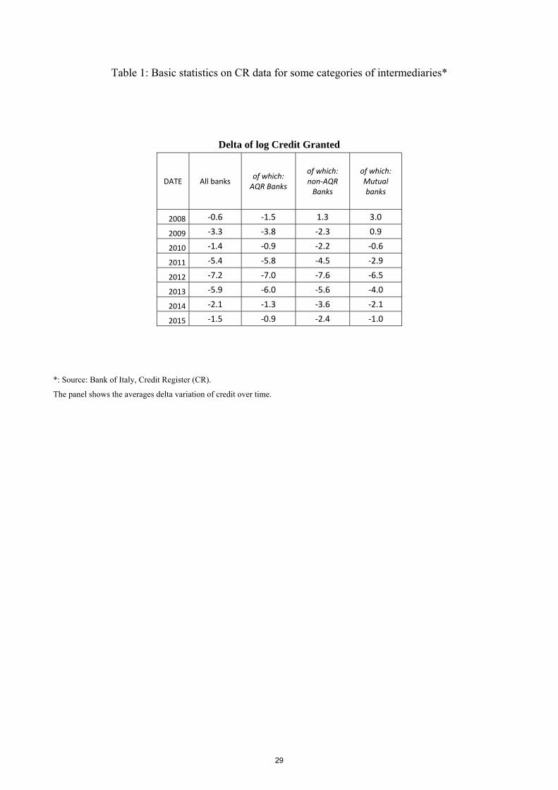
Table 1: Basic statistics on CR data for some categories of intermediaries*
Delta of log Credit Granted
DATE All banks of which: AQR Banks
of which: non-AQR
Banks
of which: Mutual banks
2008 -0.6 -1.5 1.3 3.0
2009 -3.3 -3.8 -2.3 0.9
2010 -1.4 -0.9 -2.2 -0.6
2011 -5.4 -5.8 -4.5 -2.9
2012 -7.2 -7.0 -7.6 -6.5
2013 -5.9 -6.0 -5.6 -4.0
2014 -2.1 -1.3 -3.6 -2.1
2015 -1.5 -0.9 -2.4 -1.0
*: Source: Bank of Italy, Credit Register (CR).
The panel shows the averages delta variation of credit over time.
29
Table 2: Bank characteristics*
All banks
[millions of euros and per cent]
DATE NPL
ratio
Coverage
ratio
Total
assets
T1
ratio
Leverage
ratio
Cost-income
ratio
Loan loss
provisions to
operating profit
RoE
2008 6.1 45.0 6,636 7.6 6.9 66.6 48.1 5.0
2009 9.0 39.5 6,836 8.9 7.1 61.7 60.4 4.1
2010 9.8 39.7 6,918 9.3 7.3 65.4 59.8 3.9
2011 11.0 39.8 6,964 10.1 7.5 67.6 66.6 -10.2
2012 13.2 39.3 7,138 11.1 7.1 60.9 80.4 -0.2
2013 15.9 41.7 6,725 11.1 7.1 65.7 128.8 -9.4
2014 17.7 44.5 6,706 12.3 7.1 62.0 102.1 -2.1
2015 18.1 45.4 6,696 12.7 7.2 63.7 70.3 2.7
of which
AQR banks
[millions of euros and per cent]
DATE NPL
ratio
Coverage
ratio
Total
assets
T1
ratio
Leverage
ratio
Cost-income
ratio
Loan loss
provisions to
operating profit
RoE
2008 6.3 46.1 158,367 6.9 6.6 66.9 50.0 5.2
2009 9.5 40.1 162,523 8.3 6.8 60.9 62.5 4.4
2010 10.1 40.4 166,710 8.8 7.0 64.7 60.5 4.3
2011 11.4 40.5 167,514 9.7 7.2 67.9 70.2 -13.9
2012 13.5 40.0 170,980 10.8 6.9 60.5 82.9 -0.9
2013 16.4 42.8 159,714 10.5 6.8 67.7 147.0 -12.8
2014 18.3 45.2 157,863 11.7 6.9 63.6 111.9 -3.6
2015 18.5 45.5 158,582 12.2 7.0 64.8 67.5 3.0
30
of which
non-AQR banks
[millions of euros and per cent]
DATE NPL
ratio
Coverage
ratio
Total
assets
T1
ratio
Leverage
ratio
Cost-income
ratio
Loan loss
provisions to
operating profit
RoE
2008 5.5 39.7 1,268 10.4 8.5 65.5 41.4 4.5
2009 7.3 36.7 1,392 10.9 8.3 64.9 50.8 3.2
2010 8.5 36.8 1,382 11.2 8.7 68.2 56.8 2.2
2011 9.7 36.8 1,440 11.5 8.6 66.5 54.4 2.5
2012 12.1 36.4 1,540 12.0 8.1 62.0 71.4 2.1
2013 14.2 37.4 1,533 12.9 7.8 59.3 82.5 0.9
2014 15.8 41.6 1,576 14.0 8.0 57.6 78.6 2.2
2015 16.8 44.9 1,576 14.5 8.2 60.3 77.7 1.7
of which
MUTUAL banks
[millions of euros and per cent]
DATE NPL
ratio
Coverage
ratio
Total
assets
T1
ratio
Leverage
ratio
Cost-income
ratio
Loan loss
provisions to
operating profit
RoE
2008 6.6 25.1 456 14.1 11.1 60.3 26.2 6.4
2009 8.0 24.0 495 14.5 10.9 68.3 43.3 3.8
2010 8.8 24.1 518 14.5 10.7 71.2 49.3 2.1
2011 10.3 24.8 545 14.3 10.3 68.1 55.5 2.0
2012 13.3 25.5 605 14.4 9.6 59.3 70.1 2.5
2013 16.1 30.5 638 14.7 9.1 57.4 91.3 0.5
2014 17.7 36.1 678 16.4 8.4 51.4 80.4 1.9
2015 19.1 39.8 670 16.8 8.5 56.5 88.9 -0.1
*: Source: Bank of Italy, supervisory reports.
NPL ratio is the ratio of non-performing loans to total loans. Coverage ratio is the ratio of loan loss provisions to non-performing
loans. Total assets is an average value in millions of euros. T1 ratio is the ratio of tier 1 capital to risk-weighted assets. Leverage
ratio is the ratio of equity to total assets. Cost-income ratio is the ratio of operational expenses to gross income. Loan loss provisions
to operating profit is the ratio of loan loss provisions to income net of operating expenses. RoE is the ratio of net profit to equity.
31
Table 3: Net NPL ratio (1) (2) (3) (4) (5) (6) VARIABLES No fixed
effects Firm fixed
effects Firm*time
Fixed effects Firm*time FE
Relationship ctrls Firm*time FE
Relationship ctrls Bank fixed effects
Firm*time FE Relationship ctrls Bank*firm fixed
effects Net NPL ratio 0.0741 -0.287*** 0.0282 -0.0605 -0.0650 -0.206 (0.0667) (0.0735) (0.0759) (0.0770) (0.129) (0.133) Drawn over granted -0.0162*** -0.0113*** -0.00584 (0.00348) (0.00267) (0.00478) Share of Overdraft 0.0999*** 0.0929*** 0.199*** (0.00432) (0.00357) (0.00925) Share of Total Granted -0.308*** -0.323*** -1.898*** (0.0135) (0.0125) (0.0272) Constant -4.203*** (0.530) Observations 911174 910124 897844 897844 897841 845230 R-squared 0.000 0.092 0.351 0.374 0.376 0.579
Robust standard errors in parentheses *** p<0.01, ** p<0.05, * p<0.1
32
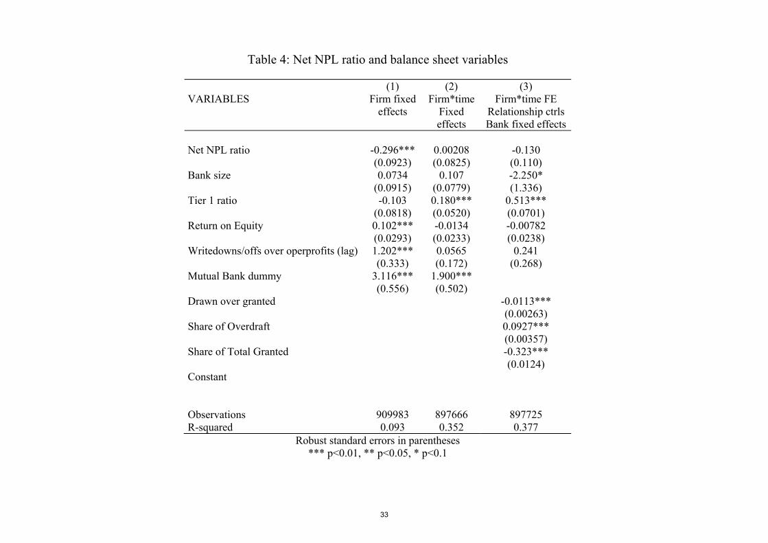
Table 4: Net NPL ratio and balance sheet variables
(1) (2) (3) VARIABLES Firm fixed
effects Firm*time
Fixed effects
Firm*time FE Relationship ctrls Bank fixed effects
Net NPL ratio -0.296*** 0.00208 -0.130 (0.0923) (0.0825) (0.110) Bank size 0.0734 0.107 -2.250* (0.0915) (0.0779) (1.336) Tier 1 ratio -0.103 0.180*** 0.513*** (0.0818) (0.0520) (0.0701) Return on Equity 0.102*** -0.0134 -0.00782 (0.0293) (0.0233) (0.0238) Writedowns/offs over operprofits (lag) 1.202*** 0.0565 0.241 (0.333) (0.172) (0.268) Mutual Bank dummy 3.116*** 1.900*** (0.556) (0.502) Drawn over granted -0.0113*** (0.00263) Share of Overdraft 0.0927*** (0.00357) Share of Total Granted -0.323*** (0.0124) Constant Observations 909983 897666 897725 R-squared 0.093 0.352 0.377
Robust standard errors in parentheses *** p<0.01, ** p<0.05, * p<0.1
33
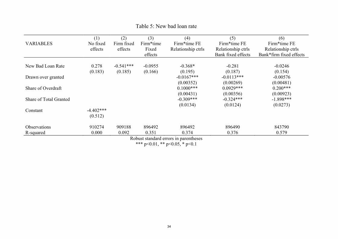
Table 5: New bad loan rate
(1) (2) (3) (4) (5) (6) VARIABLES No fixed
effects Firm fixed
effects Firm*time
Fixed effects
Firm*time FE Relationship ctrls
Firm*time FE Relationship ctrls Bank fixed effects
Firm*time FE Relationship ctrls
Bank*firm fixed effects New Bad Loan Rate 0.278 -0.541*** -0.0955 -0.368* -0.281 -0.0246 (0.183) (0.185) (0.166) (0.195) (0.187) (0.154) Drawn over granted -0.0167*** -0.0113*** -0.00576 (0.00352) (0.00269) (0.00481) Share of Overdraft 0.1000*** 0.0929*** 0.200*** (0.00431) (0.00356) (0.00923) Share of Total Granted -0.309*** -0.324*** -1.898*** (0.0134) (0.0124) (0.0273) Constant -4.402*** (0.512) Observations 910274 909188 896492 896492 896490 843790 R-squared 0.000 0.092 0.351 0.374 0.376 0.579
Robust standard errors in parentheses *** p<0.01, ** p<0.05, * p<0.1
34

Table 6: AQR and non-AQR banks
(1) (2) (3) (4) VARIABLES AQR bank 5.343*** 12.12*** (1.543) (4.032) AQR bank * post AQR 8.702*** 8.911*** 4.110 0.905 (2.738) (2.785) (5.796) (6.848) NPL ratio 0.151 0.779** (0.205) (0.379) Npl ratio * post AQR -0.115 -0.253 (0.161) (0.197) Npl ratio * AQR bank -0.977** -3.109** (0.493) (1.513) Npl ratio * AQR bank * post AQR 0.713 1.679* (0.651) (0.943) Relationship level controls yes yes yes yes Firm*Time fixed effects Bank fixed effects
yes no
yes yes
yes no
yes yes
Observations 633978 633968 595319 595316 R-squared 0.423 0.429 0.429 0.433
Robust standard errors in parentheses *** p<0.01, ** p<0.05, * p<0.1
35
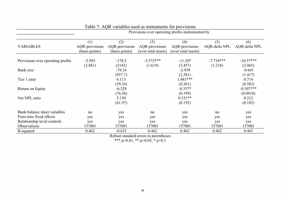
Table 7: AQR variables used as instruments for provisions
Provisions over operating profits instrumented by (1) (2) (3) (4) (5) (6) VARIABLES AQR-provisions
(basis points) AQR-provisions
(basis points) AQR-provisions (over total assets)
AQR-provisions (over total assets)
AQR-delta NPL AQR-delta NPL
Provisions over operating profits -3.993 -178.3 -5.572*** -11.28* -7.710*** -10.37*** (2.881) (2142) (1.619) (5.457) (1.218) (2.065) Bank size -78.16 -2.939 -0.641 (957.7) (2.381) (1.417) Tier 1 ratio 6.113 1.481*** 0.714 (59.34) (0.301) (0.583) Return on Equity -6.329 -0.357* -0.307*** (76.56) (0.199) (0.0910) Net NPL ratio 5.130 0.531** 0.212 (61.97) (0.192) (0.185) Bank balance sheet variables no yes no yes no yes Firm time fixed effects yes yes yes yes yes yes Relationship level controls yes yes yes yes yes yes Observations 157001 157001 157001 157001 157001 157001 R-squared 0.462 -0.632 0.462 0.462 0.462 0.463
Robust standard errors in parentheses *** p<0.01, ** p<0.05, * p<0.1
36
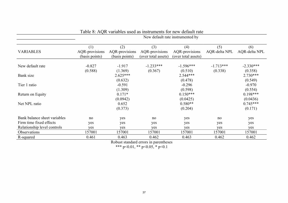
Table 8: AQR variables used as instruments for new default rate New default rate instrumented by (1) (2) (3) (4) (5) (6) VARIABLES AQR-provisions
(basis points) AQR-provisions
(basis points) AQR-provisions (over total assets)
AQR-provisions (over total assets)
AQR-delta NPL AQR-delta NPL
New default rate -0.827 -1.917 -1.233*** -1.596*** -1.713*** -2.330*** (0.588) (1.369) (0.367) (0.510) (0.338) (0.358) Bank size 2.625*** 2.544*** 2.730*** (0.632) (0.478) (0.549) Tier 1 ratio -0.591 -0.296 -0.970 (1.309) (0.598) (0.554) Return on Equity 0.171* 0.150*** 0.198*** (0.0942) (0.0425) (0.0436) Net NPL ratio 0.652 0.580** 0.745*** (0.373) (0.204) (0.171) Bank balance sheet variables no yes no yes no yes Firm time fixed effects yes yes yes yes yes yes Relationship level controls yes yes yes yes yes yes Observations 157001 157001 157001 157001 157001 157001 R-squared 0.461 0.463 0.462 0.463 0.462 0.462
Robust standard errors in parentheses *** p<0.01, ** p<0.05, * p<0.1
37

Appendix
Panel 1*
Average Share of Total Credit from each Bank
DATE All banks of which: AQR Banks
of which: non-AQR
Banks
of which: Mutual banks
2008 31.4 31.8 30.5 34.2
2009 34.9 35.0 34.7 38.9
2010 35.1 35.2 34.9 39.0
2011 34.8 34.8 34.9 39.1
2012 34.7 34.7 34.5 38.9
2013 34.6 34.7 34.6 39.1
2014 34.7 34.9 34.2 38.9
2015 34.6 35.0 33.9 38.8
Panel 2*
Drawn Credit over Granted Credit
DATE All banks of which: AQR Banks
of which: non-AQR
Banks
of which: Mutual banks
2008 71.8 76.4 62.6 60.8
2009 67.8 70.0 63.8 61.8
2010 68.3 69.9 65.3 63.6
2011 68.8 69.5 67.5 66.1
2012 72.8 75.3 68.3 67.3
2013 69.6 70.9 67.5 66.4
2014 90.1 103.6 66.3 65.4
2015 69.4 71.7 65.3 64.2
38
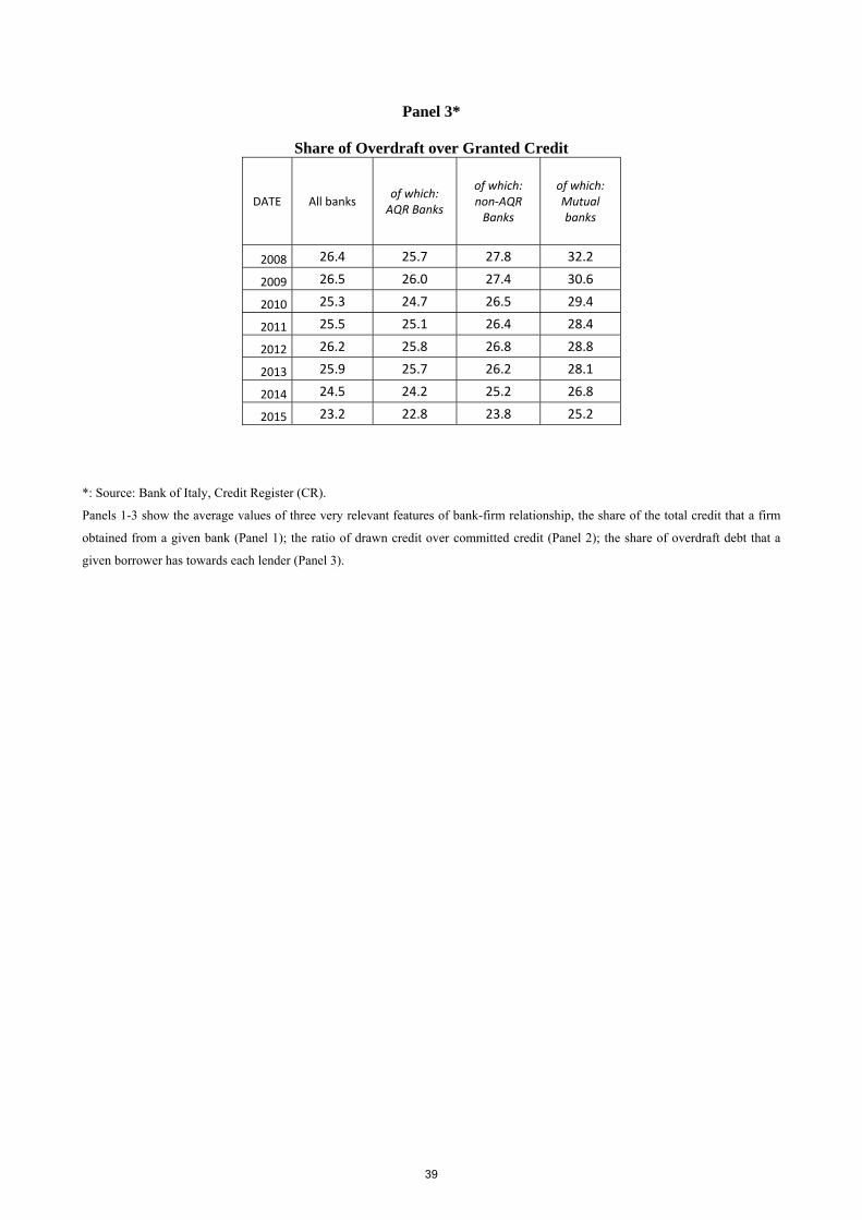
Panel 3*
Share of Overdraft over Granted Credit
DATE All banks of which: AQR Banks
of which: non-AQR
Banks
of which: Mutual banks
2008 26.4 25.7 27.8 32.2
2009 26.5 26.0 27.4 30.6
2010 25.3 24.7 26.5 29.4
2011 25.5 25.1 26.4 28.4
2012 26.2 25.8 26.8 28.8
2013 25.9 25.7 26.2 28.1
2014 24.5 24.2 25.2 26.8
2015 23.2 22.8 23.8 25.2
*: Source: Bank of Italy, Credit Register (CR).
Panels 1-3 show the average values of three very relevant features of bank-firm relationship, the share of the total credit that a firm
obtained from a given bank (Panel 1); the ratio of drawn credit over committed credit (Panel 2); the share of overdraft debt that a
given borrower has towards each lender (Panel 3).
39