Complex Systems 1 (1987) 923-938

Quantum Fractals

Siamak Amir-AziziAnthony J. G. HeyTimothy R. Morris

Department of Electronics and Computer Science,University of Southa.mpton, South amp ton 509 5NH, England

Abstract. T he fractal natu re of quantum paths contributing to Feyn­man path integral formul ation of Quantum mechanics is investigated.A comp ute r simula t ion of both one- and two-dimensional qu antumharmonic oscilla.tors yields resul ts in agreement wit h rigorou s resultson the Hausdorff-Besicovitch dimension for Brownian motion .

1. Introduction

It is well known that classical mechanics can be reformul ated in terms ofa min imum pr inciple. Th e Euler-Lagrange equ ations of mot ion follow fromdemanding tha t th e actio n

tS[x( t») = L(x , x)dt"

be stat iona ry with resp ect to va riat ions in the path x( t) taken betweenx(t j) = Xj and x( t /) = xI' An alternative formulat ion of quantum me­chanics, due to Feynman [1], is in terms of a kernel, F(x"t/; Xj ,ti), definedby

'Ii (x"t, ) = JdXiF(X"t' iXi, t;) 'Ii (Xi,t i)

T he kerne l is expresse d as a "path integra l": the path integral sums over a llpossible t rajectories x(t) from X(ti) = Xi to x(t,) = X, wit h an ampli tu dewhich depend s on the classica.l action for that path. Formally, th is is wri t tenas

r£(I,) = Xj iF( x"t'i xi ,ti) = (canst) J r ( .; )=r ; V x(t) exp[/iS[x(t)]]

where th e symbo l 'Dx(t ) is Feynman 's famous "sum over all pa th s", and theoverall constant does not concern us here. The sum over all paths may bedefined more precisely by int rod ucing a time lattice and dividing up the timeinterval , t f - t i, into equal t ime slices, e apa rt, and integra tin g over all X n ateach t ime slice In'

© 1987 Complex Systems Pub licat.ions , Inc.

924 s. Amir-Azizi, A. J. G. Hey, and T. R. Morris

where N = (t f - t;)/ c. The limit as N --> 00 defines th e pat h integral. Moredetails on pa th integr als and the relat ions hip to the Trotter pro duct formulaare to be found in the book by Schulman [2) .

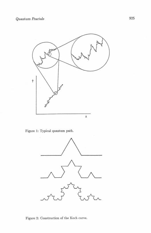
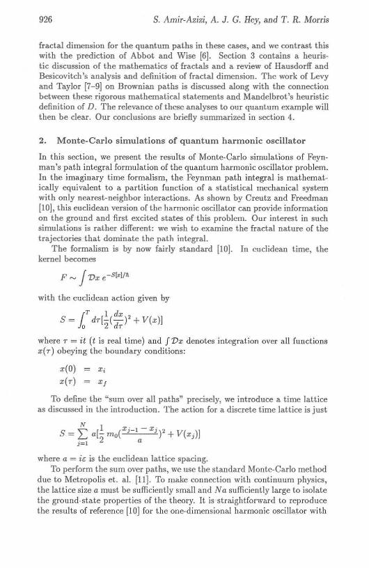
In thi s pap er , we are more concern ed with the question of which path sar e most impor tant in this path int egral. The class ical path correspondsto a minimum of the act ion, and since 6S is zero for small va riations 8x(t)about th e classical tr aj ect ory xc(t ), t hese paths interfere construct ively an ddominate the path integral as 1i -jo O. However, as observed by Feynma nand Hibbs (see figur e 1 taken from [1]), quantum mechanica l paths are veryirregu lar . Furtherm ore, as indicated in the figure, when obser ved at a finerresolution, t hey ap pear ju st as irregular as on the coarser resolu tion . Infact , t he pa th s a re everyw here contin uous but nowhere differenti ab le . T hisis the characteristic behavior of a fract al [3} and mathematicians, in par ticu­lar Hausdorff and Besicovitch [4,5], have investi gated th e propert ies of suchcu rves extensively. The classical example of a frac tal is th e so-called Kochcurve, which is cons t ructed by th e seque nce of steps shown in figure 2. Ateach increase in resolu tion by a facto r of 3, the length of th e curve increasesby 4/3. It is clear tha t the measured length of t his curve will depend on theresolut ion of our measuring instruments: the normal definition of length istherefore not very helpful for such objects. A modified definit ion of length forsuch self-simila r curves, the so-called fractal lengt h L , has been introducedby Mand elbrot [3J as

L = f(~x)D-l

where £ is the usual length measured when resolut ion is ~x and D , the fract aldimension , is a number chosen so that L will be independent of ~x in thelim it .6.x --+ O. (We will give a mathematically more precise defini t ion offra ct al dimension later in th e paper .) Not ice that for differen t iabl e curveswhose length , l, is independent of ~x, D reduces to one, the usual to po logicaldimension of a line. For the Koch cur ve, however, for two successive stepsf , = 4/3e, and ~x, = ~ (~x, ). Thus, demanding that the fractal lengt h Lbe independ ent of ~x yields the result D = f n4/ fn3 '" 1.2618.

Having obse rved th a t paths cont ribut ing to the path integral are con­tin uous but non-differentiable , one is naturally led to ask whether one candetermine a fractal dim ension for these paths . It is t his question which weset out to answer in thi s paper, and along t he way, we clar ify the connec­tion between qu antum mechan ics an d Brownian motio n, an d bet ween t hefract al dim ension of Mandelbrot and th e Hau sdorff-Besicovitch dimension ofmathemat icians.

T he pape r is constructed as follows. In th e next section, we discu ssMonte-Carlo simulat ions of quantum mechanics and exp licit ly ana lyze theproblem of one- and two-dimensional harmoni c oscillators using a euclideanvers ion of the path integral. Ou r da ta allows us to determine the relevant

Quantum Fractals

F igure 1: Typical quant um pat h.

Figure 2: Cons truction of t he Koch cu rve.

925

926 s. Amir-Azizi, A. J. G. Hey, and T. R. Morris

fractal dimension for the quantum paths in th ese cases. and we cont ras t thiswith th e prediction of Abbot and Wise (6). Section 3 contains a heuris­t ic discussion of the mathematics of fra ctals and a review of Hau sdorff andBesicovitch 's analysis and defini tion of fractal dimension. The wor k of Levyand Taylor [7- 9] on Brownian pa ths is discussed along with th e connectionbetween th ese rigorous mathematical state ments and Mandelbrot 's heuristicdefinition of D. The relevance of these analyses to OUf quantum example willth en be clear . O Uf conclusions are briefly summ arized in section 4.

2. Monte-Car lo s im ulat ions of qua ntum ha rm onic oscilla t or

In th is section, we present th e results of Monte-Carlo simu lations of Feyn­man's path integral formul ation of the quant um harm onic oscillator problem.In the imaginary time formali sm, the Feynman path integral is mathemat ­icaUy equivalent to a partit ion function of a stat ist ical mechan ical systemwith only nearest-neighbor interactions. As shown by Creutz and Freedman[10] , this euclidean version of the harmonic oscillator can provide informationon the grou nd and first excited states of this prob lem. Our interest in suchsimulat ions is ratber different: we wish to examine the fractal nature of thet rajectories t hat domin ate the path integral.

The formalism is by now fairly standard [IOJ. In euclidean time, thekernel becomes

F ~ JVx <-S«l/h

with the euclidean act ion given by

rT I dxS = Jo dr[2"(dr)' + Vex)]

where T = it (t is real t ime) and fVx denotes integrat ion over all funct ionsx(T) obeying the boundary condit ions:

x(O) = X;

x( r ) X J

To define the "sum over all paths" precisely, we introduce a time latti ceas discussed in the introdu ctio n. Th e action for a discrete t ime lat tice is just

N

S = L: a [~ mo(Xi- 'a- Xi)' + V (x;)J)=1

where a = ie is the euclidea n lattice spacing.To per form t he sum over paths, we use the standard Monte-Carlo method

due to Metropolis et . al. [I I]. To make connection with conti nuum physics,the lat t ice size a must be suffi ciently small and Na sufficiently large to isolatethe grou nd-state properties of the theory. It is st raightforward to reproducethe results of reference [10] for the one-dimensional harmoni c oscillator with

Quantum Fractals 927

1 ,V(x ) = 2 JlX .

To investigate the fractal charact er of the dominant paths cont ribut ingto th e path integral , we need to examine the varia tion in length of thesepaths as we vary the "resolut ion" of each simulat ion. Thus, for fixed t = Na ,we varied N an d a and calculated the average path length s as a funct ion ofa = Sr, Then, according to Mandelbrot's formu la

L = t(t>x)D-l

a plot of tn (t ) versus tn(t>T) has a slope of (1 - Dj , ena bling Mandelbrot 'sfract al dimension D to be determined.

T he numerical simulat ions were carried out on a number of IeL com­puters: the P ERQ and the 2970 at Southampton and the Dist ributed ArrayProcessor (DAP) at QMC London. A thermalizat ion t ime of 50 to 60 Monte­Carlo sweeps was allowed in most simulations. Values of "a " ran ged from0.02 to 0.1. For each value of a, th e optimum value of t he Monte-Carlochan ge, .!:lxopt, was found by finding t he value which resul ted in the fas testth ermalization and t he sma llest statist ical error. We found that tlxoPt equalto (a)l/2 was a good approximation in general. For each data poi nt , we gen­erated about 8000 sweeps; however , to minimi ze the effects of corre lations inthe Monte-Carlo data, measurements were carr ied out only on every tenthsweep. To est imat e the correlat ion in the remaining data, the method ofDaniell, Hey, and Mandula [12J was used .

Our results for th e one- and two-dimensional harmonic oscillator areshown in figures 3 and 4 respect ively. In both cases, we see t hat the so­called fractal dimension D is approximately 1.5. This is in contrast to thefract al dimension D = 2 suggested by Abbo t and Wise [61 in the context ofquantum tr ajectories.

How can our results be understood ? For Brownian motion, which as wewill see, is closely related to this quantu m mechanica l problem, it can berigoro usly shown {7-9] that the fractal dimension of a Brownian graph is 1.5for one-dimensional Brownian motion bu t 2 for two- or th ree-d imensionalmotion . Our results therefore seem surprising, since we do not expect thepresence of a smooth potential Vex) in t he quantum probl em to modifythese conclusions from Brownian motion . We were therefore led to exami nein more detail th e connect ion between Mandelbrot's heuri stic definition ofD and the rigorous math ematical results available on Brownian motion andth eir relevance to the quantum mechanical problem.

3. The Hausdorff-Besicovitch d imension

T he procedure to be described was first set down by Hausdorff and Besi­covitch [4,5] and is applicable to all kinds of geometrical ob jects. Since weare prim aril y interested in Feynm an paths, we will restrict our discussionto objects of topological dimension one: generaliza t ion to higher topologicaldimensions is st raightforward.

928 S. Amir-Aaiai, A. J. G. Hey, and T. R. Morr;s

7.00

6.80

6.68D = 1 - Slope

6.10 = 1.496

:;;-6.28

1~

eoc 6.00_~

5.801

-;;;~

u~:::. 5.60~

"" 5.10

5.20

5.00

1.80

1.68 ,-7 -6 -5 _4 -3 -2,

fn( ,c"T)

Figure 3: Quantum path in one space dimension.

Quant um Fractals 929

7.00 D = 1 - Slope

6.80 \= 1.496

6.60 -,:?

6.10j\

~

'\eoQ

.2

"3 6.20 \u

6.001~~

~

e..,

S""15.60

S. ,a:5.20

5.00 , ,-7 -6 -5 -1 -3 -2

fn(tJ.T)

Figure 4: Quantum path in two space dimensions.

930 S. Amir-Azizi, A. J. G. Hey, and T. R. Morris

To determine the Hausdorff-Besicovltch (HB) dimension, we first covert he cu rve completely with a finite set of sphe res of var ious radii "'Pi" . T hesespheres may overlap. For each of these sphe res , we ca lculate the quant ity

h{Pi) = {pol"

whe re d is a real nu mber whose value is arbitrary for the moment. We thensum the results:

alp;} = L h{Pi)

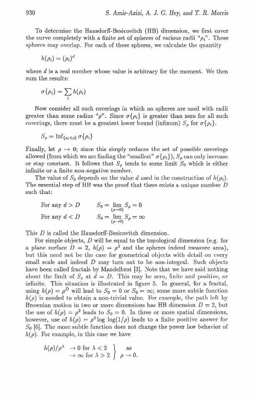
Now consider all such coverings in which no spheres arc used with radiigreater t han some radius "p". Since a{pil is. greater than zero for all suchcoverings, there must be a greatest lower bound (infinum) Sp for o- {Pi}'

F inally, let p -+ 0; since t his simply reduces the set of possib le cove ringsallowed (from which we are find ing the "smallest " a{piJ ), Sp can only increaseor stay constant . It follows that Sp te nds to some limit So which is eitherinfinite or a finite non-negative number.

The value of So dep ends on the value d used in the construction of h{pJTh e essent ial step of HB was the proof that there exists a unique number Dsuch that:

For any d > D

For any d < D

So = lim S, = 0(,_0)

So = lim S, = 00(p--+o)

Thi s D is called th e Hau sdorff-Besicovitch dimen sion .For simple ob jects, D will be equal to t he topological dimension (e.g. for

a plane surface D = 2, k(p) = p2 and the spheres indeed measure area) ,but th is need not be the case for geometrical objects wit h detail on everysmall scale and indeed D may turn out to be non-integra l. Such objectshave been called fractals by Mandelbrot [31. Note that we have said nothingabout the limit of Sp at d = D. This may be zero, finite and posit ive, orinfinite. Thi s sit uat ion is illustrated in figure 5. In general, for a fractal,using h(p) = pD will lead to So = 0 or So = 00 ; some more subt le funct ionk(p) is needed to ob tain a non-trivial value. For example, the path left byBrownian motion in two or more dimen sions has HB dimension D = 2, butthe use of h(p) = p2 leads to So = O. In th ree or more spat ial dimensions,however, use of h(p) = p' log log{l / p) leads to a finit e positi ve answer forSO[6J . T he more subtle funct ion does not change the power law behavior ofh(p). For exampl e, in th is case we have

h(p)/ pA --> 0 for A < 2} as---+ 00 for ,\ > 2 P ---+ O.

Quant um Fractals

Curve an dsimp le covering

Infinum coveringPi < P

p--+ O

931

Figure 5: Curve and simple coverings.

In a sense , the form of h(p) is indicating th at the HB dimen sion is infinites­imally less than two [3] since in fact:

h(p)/p ' --+ 00 for ), 2: 2 as p -+ o.

It should therefore be clear that h(p) need on ly be known up to a powerin p in order to determ ine the HB dimension . The funct ion h(p) that yieldsa finite positive resul t for So at d = D is known as the int rinsic (see figure6). T he limit So is known as the measure and we see here that it depends onthe funct ion h(p).

Some simple properties of the HB dimension are intui ti vely obvious (an deas ily proved):

1. D 2 (topological dimension of th e space), e.g. for our quantum pathsD2:1.

2. D .5 (topological dimension of th e space in which th e curve is embed­ded).

3. Th e HB dimension Dp of the pro ject ion of a curve down on to a sub­space sa t isfies Dp S D (where D is the HB dimen sion of the originalcurve).

We now discuss the connect ion of the HB dimension with Mandelbrot'sheurist ic definition of a fract al dimension. Mandelbrot defines D by th eformula

L = €(a)D- l

932 S. Amir-Azizi, A. J. G. Hey, and T . R. Morris

So

OL - - --- -r== = = = ==-7(do

Figure 6: Graph of So = limp.....oSp as a function of d.

where L is a quant ity ind ep endent of t he "reso lu t ion" G , and l is t he lengthof the curve at the resolution "an. Thi s formula st rictly only holds for st a­t istical ly self-sim ila r curves-curves whose behavior looks exact ly t he same(or sta t ist ica lly the sa me) on every scale.

Su ppose tha t instead of covering the cur ve wit h spheres of va rying radiiPi ~ p, we cove r t he curve wit h spheres of all th e same radi us "c". We canst ill consider all possible such coverings and form the infinum value of thequa nti ty, L h(a), where th e sum is over all spheres in the covering. In th iscase, t herefore, we ca n define a lengt h L(J. by

L. = Inf 2:h(a)=N h(a)= Nad

where N is the minimum number of spheres of radi us a needed to cover thecurve. Now consider the limit Lo of (N ad) as a -j. O. Since

we have

Lo 2 lim 5. = 50(0.-0)

Moreover , it is clea r that there must be some value D' such that

for allfor a ll

d > D', Lo = 0 whiled < D', Lo = 00 .

Quant um Fractals 933

T he inequa lity above th en imp lies th at D' 2: D.We may reformulate this definit ion of length and fract al dimension D

in te rms of "res olut ions" . If "a" is the resolutio n, then, using t his infinumcovering, we would call th e length of the curve f. = No. We may then rewriteour expression for La in te rms of eand a :

L . = f (a)d-l

If, further, we only determine thi s length f. up to some power of "a", thenthere will be some value of I'd" for which La will not depend on "a" as a ---+ O.This is d = D' = D.

Hence we arr ive at

L = f (a)D- l (L independent of a)

Alt hough this formula was origina lly int rod uced by Ma nd elb rot for self­simila r curves [3], it sho uld be clear from our derivat ion that , provided wecan determine the appropriate "a" for a given approximat ion to a fract al,th is formu la may be app lied to fractals tha t ar e not self-sim ilar.

Note that, except in very simple cases, no import ance can be at tached toth e va lue of L: t he formula being derived from approximations in the coveri ngand "e" being determined only up to a power law in "a" . T he determinat ionof the HB dimension is red uced to dete rmining th e behavior of the lengt h"f." as a power law in the resolution according to f. ex: a I - D .

4. T he frac tal dimension of paths associa t ed with the path int e-gra l

As stated before , the most import ant paths cont ribut ing to the path integra lare pa th s lyin g closely around the classical path which are highly irregularand non-different iab le on all scales. The natural ap proximat ion to thesepaths is that obtained by chopping up the pat h integral into t ime slices!:1t = E . Consider the action

Jm x2

S[;(J = (:2 - V (;( )) dt ,

for I< space dimensions ~ = Xl , ... , XK). Rotat ing into eucl idean sp ace, th epa th integral is

,,\,N-l 2J'D(x ( t) ) e ~ S[x( t )ln~,;/i:dKxn

e=tLJn : 1 {~(.£n+ l -Ln) + V (~ ). }

T he ju m p, .6.x, in the x position for a t ime increment .6.t = e is given by

(L>x)' {(Ln+l-;(m)'}rrN - I foo dK x e- i L{ :¥;(1::n+ l -lZ,1 )2 +V (~ )~}( ~ _ ~ ) '

n-l 00 n ~m+I ::.lo:.m

n~=Il J~oodKXne kL)¥;~+l ~)2 +V (~)~ }

Clearly, as e ---+ 0, the po tent ial ter m becomes unimportant and th e integralsfactorize. Hence, we ob tain (for sufficient ly small s ) the well-known resultthat

934 S. Amir-Azizi, A. J. G. Hey, and T. R. Morris

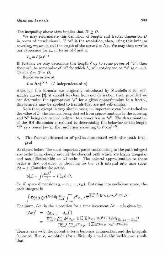
time

2E I-~=----------

~1

/~o

(

Figure 7: The graph.

!J.. x ......, c l / 2

)

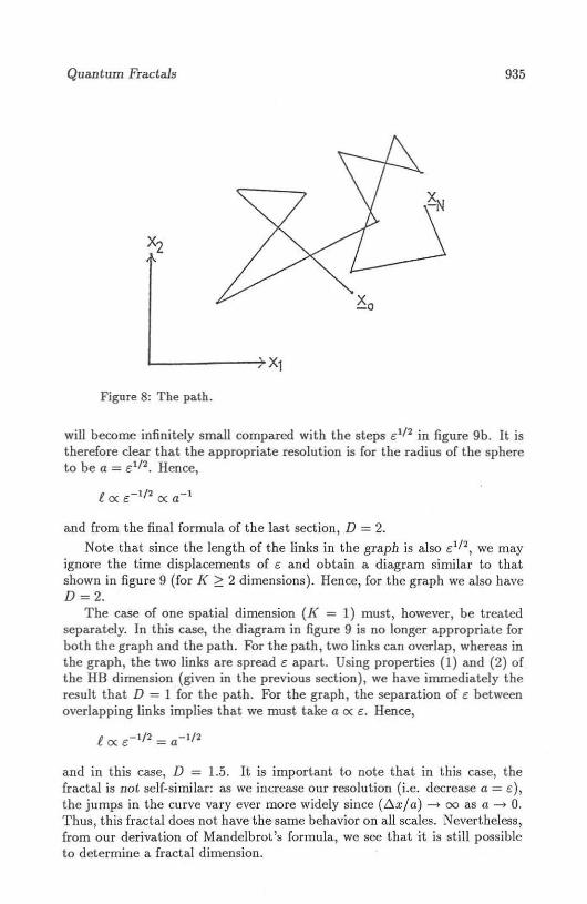
This formula is sufficient to determine the fractal dimension of both thegraph, a plot of ;r(t ) against time (see fignre 7), and the path , the trace leftin [{-space as time evolves (see figure 8) . Notice that the length of a link inboth the graph and t he path is , 1/2 (since e « , 1/2 for' ---> 0). This meansthat the total length of both graph and pat h for time slice t:>t = e may bedefined as l = N e l / 2 = (Tie) e1/ 2 = T e- 1/ 2 (wbere T is the total t ime).

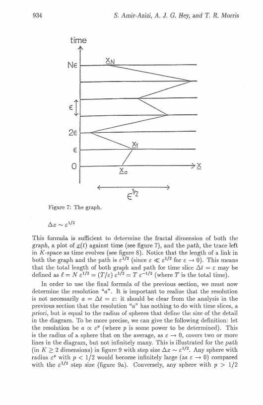
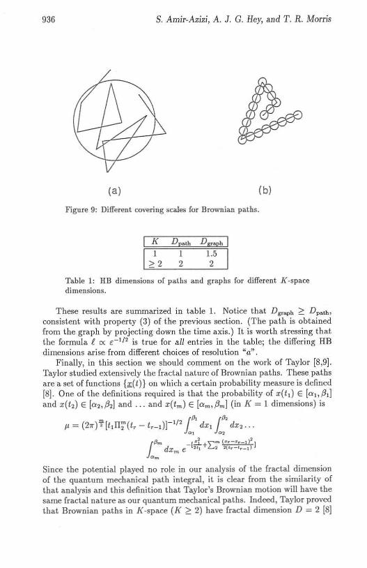
In order to use the final formula of the previous section, we must nowdetermine the resolution "an . It is important to realize that the resolutionis not necessarily a = ilt = s : it should be clear from the analysis in theprevious section that the resolu tion "a" has nothing to do with time slices , a.priori, but is equal to the radius of spheres that define the size of the detailin the diag ram. To be more precise, we can give the following definition: letthe resolution be a ex: £11 (where p is some power to be determined). Thisis the radius of a sphere that on the average, as e --+ 0, covers two or morelines in the diagram, but not infinitely many_ This is illustrated for the path(in J( ~ 2 dimensions) in figure 9 with step size ~x rv e1/ 2 . Any sphere withradius e with p < 112 would become infinitely large (as e ---> 0) comparedwith the el / 2 step size (fi gure gal. Conversely, any sphere with p > 1/ 2

Quant um Fractals 935

l..-----.... x,Figure 8: Th e path .

will become infinitely small compared with th e steps e. 1/ 2 in figure 9b. It istherefore clear that the appropriate resolut ion is for the radius of the sphereto be a = e. 1/ 2 • Hence,

lex: e.-1/ 2 ex: a - I

and from the final formula of the last section, D = 2.

Note that since the length of the links in the graph is also e.1/2, we mayignore t he time displacements of e and obtain a diagram similar to thatshown in fi gure 9 (for J( ~ 2 dimensions). Hence, for the graph we also haveD =2.

Th e case of one spatial dimension (I< = 1) must , however, be treatedsepara tely. In th is case, the diagram in figure 9 is no longer appropriate forboth the graph and the path. For the path , two links can overlap , whereas int he graph, the two links are spread e apar t. Using prop erti es (1) and (2) ofthe HB dimension (given in the previous section) , we have immedia tely theresult t hat D = 1 for the path. For the graph , the separat ion of e betweenoverlapping links implies that we must take a ex: e. Hence,

lex: £ - 1/2 = a -1 / 2

and in this case, D = 1.5. It is important to note that in this ease, thefractal is not self-similar : as we increase our resolutio n (i.e. decrease a =s ),the jumps in the curve vary ever more widely since (f:j.x/a) .......... 00 as a -+ O.Th us, thi s fractal does not have t he same behavior on all scales. Nevertheless,from our derivation of Mandelbrot's formula, we see that it is st ill possibleto determine a fractal dimension.

936 S. Amir-Aaizi, A. J. G. Hey, and T. R. Morris

(a ) (b)

Figure 9: Different covering scales for Brownian paths.

12

Table 1: HD dim ensions of paths and graphs for different J(-spacedime nsions.

These results arc summarized in table 1. Notice that Dgraph 2: D PAlh l

consistent with property (3) of the previous sect ion. (T he path is obtainedfrom the gra ph by projecting down th e time axis.) It is worth st ressing thatthe formula e ex &-1/ 2 is t rue for all entries in the table; th e differing HBdimensions ar ise from different choices of resolution "a" .

Fi nally, in this sect ion we should comment on the work of Taylor [8,9].Taylor studied extensively the fractal nature of Brownian paths. T hese pat hsarc a set of funct ions b :.(t )} on which a certain probability measure is defined[8]. One of the definit ions required is that the probability of x(ltl E [<>hPI]an d x( I, ) E [<>"P,] an d .. . and x(lm) E [<>m,Pml (in f{ = 1 dimensions) is

'" m -1/' lP, 1!J,I' = (2,,) ' [1 111, (I, - 1,_1)] dXI dx, ...

0' 1 0'2

13m ~ m ( "' '' -''' .. 1 )2

1 d X m e-12' 1 + L:2 2( 1" _' '' _1> Ja m

Since th e potential played no role in our analysis of th e fract al dimensionof th e quantum mechanical path int egral , it is clear from t he similarity ofthat analysis and thi s definition that Taylor's Brownian motion will have thesame fract al nature as our quantum mechanical path s. Indeed, Tay lor provedt hat Brownian paths in f{ -space ( f{ ~ 2) have fractal dim ension D = 2 [8]

Quant um Fractals 937

and that the graph of a one-dimen sional Brownian path has D = 1.5 [9).In addition, he obtained information regarding the measure and intrinsic forthese cases. For K = 2, the intrinsic for the path is L(p) = p210g log log(l / p),while for J( ~ 3, the intrinsic for the path is L(p) = p2 log log(l / p). (Th emore complicated expression for J( = 2 is due to the fact that the path isable to cross over itself infinitely often.) He also showed that for J( = 1, thegraph has zero measure with h(p) = p3/2.

In view of the correspondence between Taylor's rigorous definitions ofBrownian motion and the concept of the path integral as introduced byFeynman, it is comforting to note that our heuristic analysis yields answersin agreement with his work.

5. Concl usions

We have investigated the fractal nature of the dominant paths contribut­ing to Feynman 's path integral for the quantum oscillator in both one andtwo dimensions. A naive application of Mandelbrot's formula for fractal di­mension yields D = 1.5 in both cases, in contrast to the result of Abbottand Wise, who arrived at the result D = 2 for quantum motion , albeit ina different context. More worrying was the apparent contradiction with theresults of Taylor, who predicted D = 1.5 and D = 2 for graphs of one­and two-dimensional Brownian motion respect ively. Since the quantum me­chanical case differs only byan irrelevant potential function, we would expectthese results to be true for quantum paths. However, a clearer examination ofthe connection of Mandelbrot's definition of fractal dimension shows that theappropriate resolution must be chosen with care. For the one-dimensional os­cillator, the resolution is indeed the time separation, a , and we have D = 1.5.For the two-dimensional oscillator, the appropriate resolution is a1/ 2 corre­sponding to the average step size resulting in D = 2, in agreement with thatexpected from the work of Taylor.

Refe rences

[1] R. P. Feynman and A. R. Hibbs, Quantum Mechanics and Pat h Integrals,(McGraw Hill, New York , 1965).

[2] L. S. Schulman, Techniques and Applications of Path Integration, (JohnWiley & Sons, 1981).

{3] .B. B. Mandelbrot, Fractals: Form, Chance and Dimension, (Freeman, SanFrancisco, 1977).

[4J F. Hausdorff, Math Annalen, 79 (1918) 157.

[5J A. S. Besicovitch , Journal London Matll Soc., 9 (1934) 126.

[6) L. F. Abbott and M. B. Wise, American Journal of Physics, 49: 1 (1981)37- 39.

938 S. Amir-Azjzi, A. J. G. Hey, and T. R. M orris

[7] P. Levy, Giron Inst . Ital. Attuari., 16 (1953) I.

[8] S. J . Taylor, Proc. Camb . Pb il. Soc., 49 (1953) 31.

[9] S. J . Taylor, Proc. Camb. Pbil. Soc., 51 (1955) 265.

[10] M. Creutz and B. Freedman, Pbysics, 13 2 (1981) 427.

[11] N. Metropolis, A. W. Rosenbluth, M. N. Rosenbluth, A. R. Teller, and E.TeUer, J. Cbem. Phys. , 21 (1953) 1087.

[12] G. J. DanieU, A. J. G. Hey, and J . E. Mand ala, Phys. Rev. D, 30 (1984)2230.