Quantitative Strategies Research Notes

Quantitative StrategiesResearch Notes

GoldmanSachs

The Local Volatility SurfaceUnlocking the Information in Index Option Prices

Emanuel DermanIraj KaniJoseph Z. Zou

December 1995

QUANTITATIVE STRATEGIES RESEARCH NOTESSachsGoldman

Copyright 1995 Goldman, Sachs & Co. All rights reserved.

This material is for your private information, and we are not soliciting any action based upon it. This report is not tobe construed as an offer to sell or the solicitation of an offer to buy any security in any jurisdiction where such an offeror solicitation would be illegal. Certain transactions, including those involving futures, options and high yieldsecurities, give rise to substantial risk and are not suitable for all investors. Opinions expressed are our presentopinions only. The material is based upon information that we consider reliable, but we do not represent that it isaccurate or complete, and it should not be relied upon as such. We, our affiliates, or persons involved in thepreparation or issuance of this material, may from time to time have long or short positions and buy or sell securities,futures or options identical with or related to those mentioned herein.

This material has been issued by Goldman, Sachs & Co. and/or one of its affiliates and has been approved byGoldman Sachs International, regulated by The Securities and Futures Authority, in connection with its distributionin the United Kingdom and by Goldman Sachs Canada in connection with its distribution in Canada. This material isdistributed in Hong Kong by Goldman Sachs (Asia) L.L.C., and in Japan by Goldman Sachs (Japan) Ltd. Thismaterial is not for distribution to private customers, as defined by the rules of The Securities and Futures Authorityin the United Kingdom, and any investments including any convertible bonds or derivatives mentioned in thismaterial will not be made available by us to any such private customer. Neither Goldman, Sachs & Co. nor itsrepresentative in Seoul, Korea is licensed to engage in securities business in the Republic of Korea. Goldman SachsInternational or its affiliates may have acted upon or used this research prior to or immediately following itspublication. Foreign currency denominated securities are subject to fluctuations in exchange rates that could have anadverse effect on the value or price of or income derived from the investment. Further information on any of thesecurities mentioned in this material may be obtained upon request and for this purpose persons in Italy shouldcontact Goldman Sachs S.I.M. S.p.A. in Milan, or at its London branch office at 133 Fleet Street, and persons in HongKong should contact Goldman Sachs Asia L.L.C. at 3 Garden Road. Unless governing law permits otherwise, youmust contact a Goldman Sachs entity in your home jurisdiction if you want to use our services in effecting atransaction in the securities mentioned in this material.

Note: Options are not suitable for all investors. Please ensure that you have read and understood thecurrent options disclosure document before entering into any options transactions.

-2


SUMMARY

If you examine the structure of listed index optionsprices through the prism of the implied tree model,you observe the local volatility surface of the under-lying index.

In the same way as fixed income investors analyzethe yield curve in terms of forward rates, so indexoptions investors should analyze the volatility smilein terms of local volatilities.

In this report we explain the local volatility surface,give examples of its applications, and propose sev-eral heuristic rules of thumb for understanding therelation between local and implied volatilities. Inessence, the model allows the extraction of the fairlocal volatility of an index at all future times andmarket levels, as implied by current options prices.We use these local volatilities in markets with a pro-nounced smile to measure options market senti-ment, to compute the evolution of standard optionsimplied volatilities, to calculate the index exposureof standard index options, and to value and hedgeexotic options. In markets with significant smiles, allof our results show large discrepancies from theresults of the standard Black-Scholes approach.

Investors who buy or sell standard index options forthe exposure they provide, as well as market partici-pants interested in the fair price of exotic indexoptions, should find interest in the deviations wepredict from the Black-Scholes results._______________________________

Emanuel Derman (212) 902-0129Iraj Kani (212) 902-3561Joseph Z. Zou (212) 902-9794

_______________________________

We are grateful to Barbara Dunn for comments onthe manuscript.

-1


Table of Contents

THE IMPLIED VOLATILITY SURFACE............................................................... 1

THE IMPLIED VOLATILITY SURFACEBELIES THEBLACK-SCHOLESMODEL.. 2

THE LOCAL VOLATILITY SURFACE.................................................................. 4

THE ANALOGY BETWEENFORWARD RATES AND LOCAL VOLATILITIES ........ 7

USING THELOCAL VOLATILITY SURFACE..................................................... 10

Obtaining the local volatilities ............................................................. 10

The correlation between index level and index volatility .................... 13

Implied distributions and market sentiment ........................................ 14

The future evolution of the smile ........................................................ 14

The skew-adjusted index exposure of standard options ...................... 17

The theoretical value of barrier options ............................................... 19

Valuing path-dependent options using Monte Carlo simulation ......... 20

APPENDIX: The relation between local and implied volatilities ................... 25

1


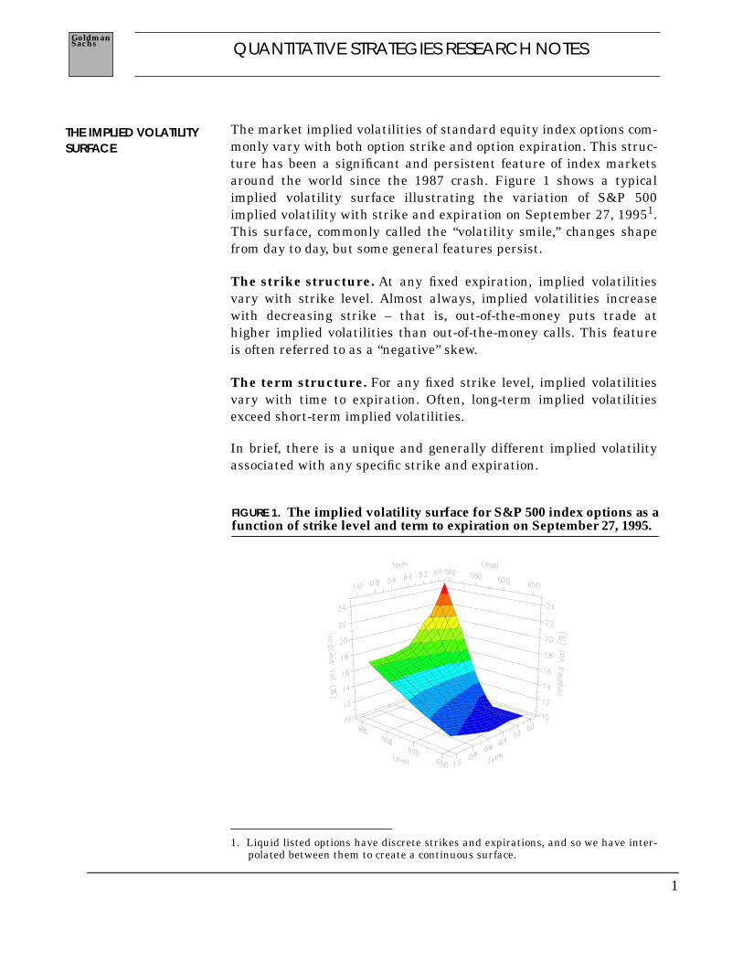
The market implied volatilities of standard equity index options com-monly vary with both option strike and option expiration. This struc-ture has been a significant and persistent feature of index marketsaround the world since the 1987 crash. Figure 1 shows a typicalimplied volatility surface illustrating the variation of S&P 500implied volatility with strike and expiration on September 27, 19951.This surface, commonly called the “volatility smile,” changes shapefrom day to day, but some general features persist.

The strike structure. At any fixed expiration, implied volatilitiesvary with strike level. Almost always, implied volatilities increasewith decreasing strike – that is, out-of-the-money puts trade athigher implied volatilities than out-of-the-money calls. This featureis often referred to as a “negative” skew.

The term structure. For any fixed strike level, implied volatilitiesvary with time to expiration. Often, long-term implied volatilitiesexceed short-term implied volatilities.

In brief, there is a unique and generally different implied volatilityassociated with any specific strike and expiration.

1. Liquid listed options have discrete strikes and expirations, and so we have inter-polated between them to create a continuous surface.

THE IMPLIED VOLATILITYSURFACE

FIGURE 1. The implied volatility surface for S&P 500 index options as afunction of strike level and term to expiration on September 27, 1995.

2


Each implied volatility depicted in the surface of Figure 1 is theBlack-Scholes implied volatility, Σ, the volatility you have to enterinto the Black-Scholes formula to have its theoretical option valuematch the option’s market price. Σ is the conventional unit in whichoptions market-makers quote prices. What does the varying volatilitysurface for Σ tell us about the model and the world it attempts todescribe?

The primary feature of the Black-Scholes [1973] model of options val-uation theory is that it is preference-free: since options can be hedged,their theoretical values do not depend upon investors’ risk prefer-ences. Therefore, an index option can be valued as though the returnon the underlying index is riskless.

A secondary feature of the theory is its assumption that returns onstocks or indexes evolve normally, with a local volatility σ thatremains constant over all times and market levels. Figure 2 contains aschematic representation of the index evolution in a binomial treeframework2. The constant index level spacing in the figure corre-sponds to the assumption of constant local return volatility. Thesetwo features leads to the Black-Scholes formula fora call on an index at level S with a volatility σ, with strike K and timeto expiration T, when the riskless interest rate is r.

2. In mathematical terms, the evolution over an infinitesimal time dt is described bythe stochastic differential equation

where S is the index level, µ is the index’s expected return and dZ is a Wienerprocess with a mean of zero and a variance equal to dt.

THE IMPLIED VOLATILITYSURFACE BELIES THEBLACK-SCHOLESMODEL

dSS

-------- µdt σdZ+=

CBS S σ r T K, , , ,( )

indexlevel

time

FIGURE 2. A schematic representation of index evolution in the Black-Scholes model.

3


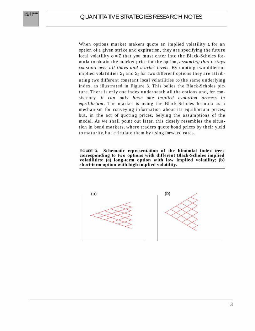
When options market makers quote an implied volatility Σ for anoption of a given strike and expiration, they are specifying the futurelocal volatility σ = Σ that you must enter into the Black-Scholes for-mula to obtain the market price for the option, assuming that σ staysconstant over all times and market levels. By quoting two differentimplied volatilities Σ1 and Σ2 for two different options they are attrib-uting two different constant local volatilities to the same underlyingindex, as illustrated in Figure 3. This belies the Black-Scholes pic-ture. There is only one index underneath all the options and, for con-sistency, it can only have one implied evolution process inequilibrium. The market is using the Black-Scholes formula as amechanism for conveying information about its equilibrium prices,but, in the act of quoting prices, belying the assumptions of themodel. As we shall point out later, this closely resembles the situa-tion in bond markets, where traders quote bond prices by their yieldto maturity, but calculate them by using forward rates.

FIGURE 3. Schematic representation of the binomial index treescorresponding to two options with different Black-Scholes impliedvolatilities: (a) long-term option with low implied volatility; (b)short-term option with high implied volatility.

(a) (b)

4


There is a simple extension to the strict Black-Scholes view of theworld that can achieve consistency with the index market’s impliedvolatility surface, without losing many of the theoretical and practi-cal advantages of the Black-Scholes model.

Rational market makers are likely to base options prices on theirestimates of future volatility3. To them, the Black-Scholes Σ is,roughly speaking, a sort of estimated average future volatility of theindex during the option’s lifetime. In this sense, Σ is a global measureof volatility, in contrast to the local volatility σ at any node in the treeof index evolution. Until now, theory has tended to disregard the dif-ference between Σ and σ. Our path from now on is to accentuate thisdifference, and deduce the market’s expectations of local σ from thevalues it quotes for global Σ.

The variation in market Σ indicates that the average future volatilityattributed to the index by the options market depends on the strikeand expiration of the option. A quantity whose average varies withthe range over which it’s calculated must itself vary locally. The vari-ation in Σ with strike and expiration implies a variation in σ withfuture index level and time. In other words, the implied volatilitysurface suggests an obscure, hitherto hidden, local volatility surface.

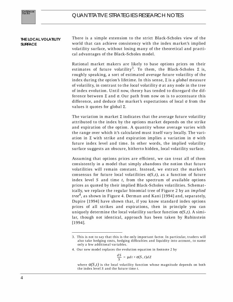
Assuming that options prices are efficient, we can treat all of themconsistently in a model that simply abandons the notion that futurevolatilities will remain constant. Instead, we extract the market’sconsensus for future local volatilities σ(S,t), as a function of futureindex level S and time t, from the spectrum of available optionsprices as quoted by their implied Black-Scholes volatilities. Schemat-ically, we replace the regular binomial tree of Figure 2 by an impliedtree4, as shown in Figure 4. Derman and Kani [1994] and, separately,Dupire [1994] have shown that, if you know standard index optionsprices of all strikes and expirations, then in principle you canuniquely determine the local volatility surface function σ(S,t). A simi-lar, though not identical, approach has been taken by Rubinstein[1994].

3. This is not to say that this is the only important factor. In particular, traders willalso take hedging costs, hedging difficulties and liquidity into account, to nameonly a few additional variables.

4. Our new model replaces the evolution equation in footnote 2 by

where σ(S,t) is the local volatility function whose magnitude depends on boththe index level S and the future time t.

THE LOCAL VOLATILITYSURFACE

dSS

-------- µdt σ S t,( )dZ+=

5


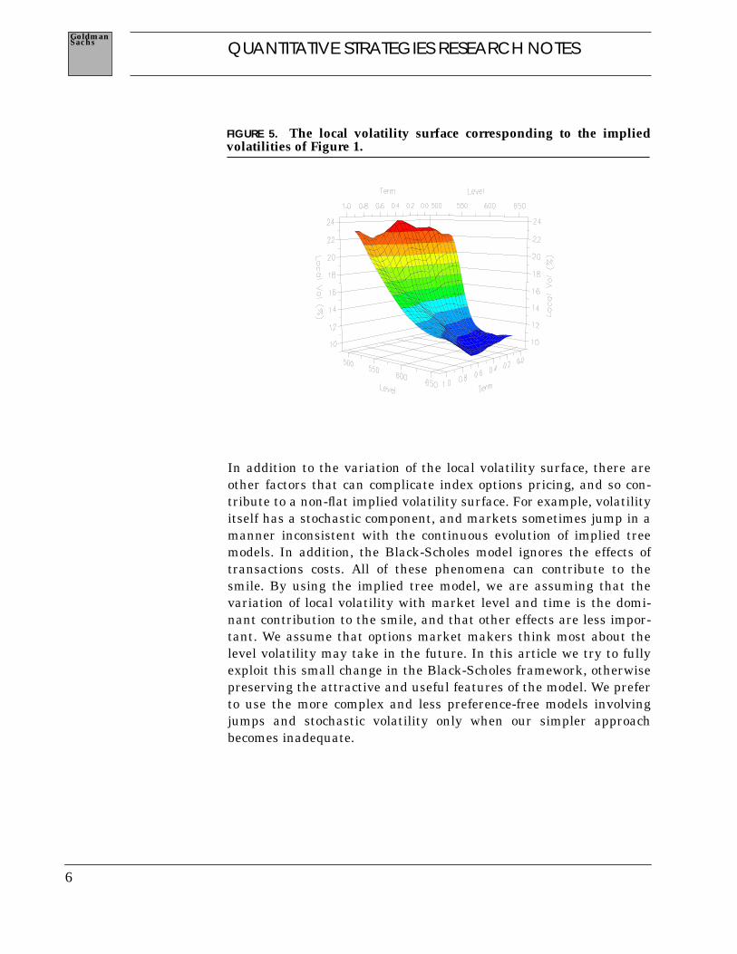
In essence, our model assumes that index options prices (that is,implied volatilities) are driven by the market’s view of local index vol-atility in the future. We have shown that you can theoretically extractthis view of the local volatility σ(S,t) from standard options prices.Readers familiar with the habits of options traders will realize thatthinking about future volatility is an intrinsic part of their job. Manytraders intuitively deduce future local volatilities from options prices.Our model provides a more quantitative and exact way of accomplish-ing this. Figure 5 displays the local volatility surface corresponding tothe implied volatility surface of Figure 1.

Our approach preserves many of the attractive facets of the Black-Scholes model, while extending it to achieve consistency with marketoptions prices. The great advantage of the Black-Scholes model in atrading environment is that it provides preference-free pricing. Itsinputs are current index levels, estimated dividend yields and inter-est rates, most of which are determined and well-known. All themodel asks of a user is one implied volatility, which it translates intoan option price, an index exposure, and so on.

The implied tree model preserves this quality. In brief, all it asks of auser is the implied Black-Scholes volatility of several liquid options ofvarious strikes and expirations. The model fits a consistent impliedtree to these prices, and then allows the calculation of the fair valuesand exposures of all (standard and exotic) options, consistent with allthe initial liquid options prices. Since traders know (or have opinionsabout) the market for current liquid standard options, this makes itespecially useful for valuing exotic index options consistently withthe standard index options used to hedge them.

indexlevel

time

FIGURE 4. The implied binomial tree.

6


In addition to the variation of the local volatility surface, there areother factors that can complicate index options pricing, and so con-tribute to a non-flat implied volatility surface. For example, volatilityitself has a stochastic component, and markets sometimes jump in amanner inconsistent with the continuous evolution of implied treemodels. In addition, the Black-Scholes model ignores the effects oftransactions costs. All of these phenomena can contribute to thesmile. By using the implied tree model, we are assuming that thevariation of local volatility with market level and time is the domi-nant contribution to the smile, and that other effects are less impor-tant. We assume that options market makers think most about thelevel volatility may take in the future. In this article we try to fullyexploit this small change in the Black-Scholes framework, otherwisepreserving the attractive and useful features of the model. We preferto use the more complex and less preference-free models involvingjumps and stochastic volatility only when our simpler approachbecomes inadequate.

FIGURE 5. The local volatility surface corresponding to the impliedvolatilities of Figure 1.

7


The implied-tree approach to modeling the volatility smile stressesthe use of local volatilities extracted from implied volatilities. Ourincentive to analyze value in terms of local quantities rather thanglobal averages is analogous to a similar historical development inthe analysis of fixed income securities more than a generation ago.

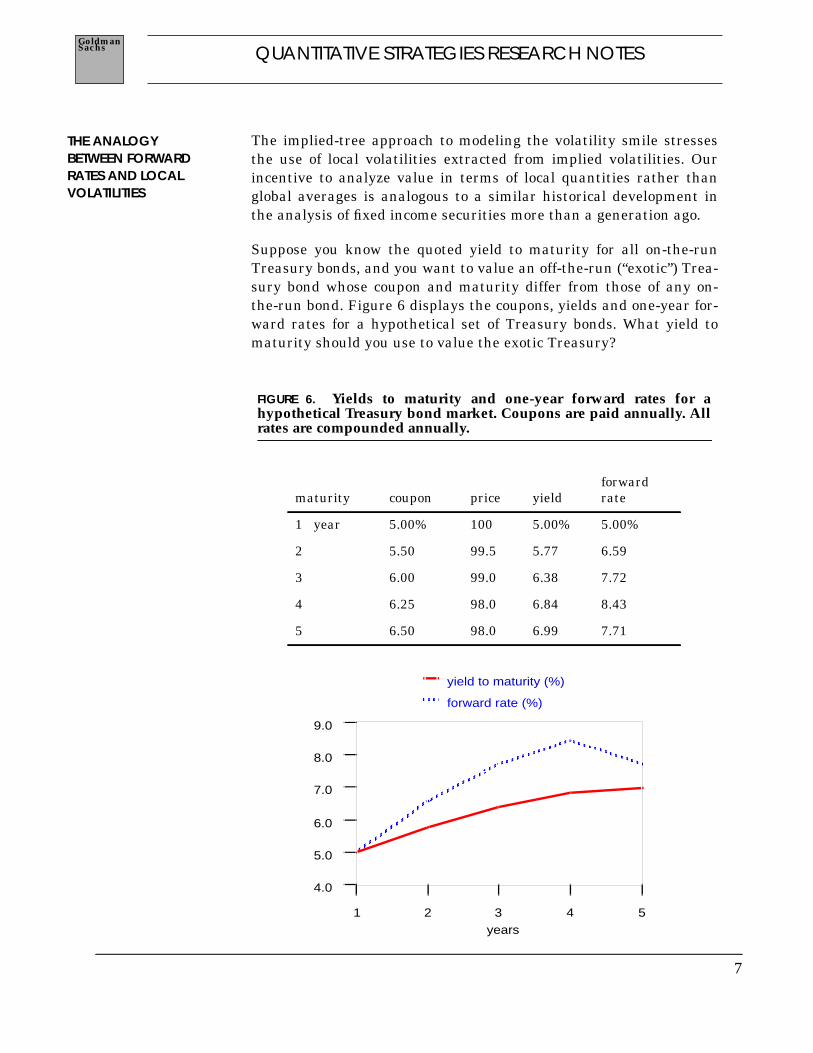
Suppose you know the quoted yield to maturity for all on-the-runTreasury bonds, and you want to value an off-the-run (“exotic”) Trea-sury bond whose coupon and maturity differ from those of any on-the-run bond. Figure 6 displays the coupons, yields and one-year for-ward rates for a hypothetical set of Treasury bonds. What yield tomaturity should you use to value the exotic Treasury?

THE ANALOGYBETWEEN FORWARDRATES AND LOCALVOLATILITIES

FIGURE 6. Yields to maturity and one-year forward rates for ahypothetical Treasury bond market. Coupons are paid annually. Allrates are compounded annually.

maturity coupon price yieldforwardrate

1 year 5.00% 100 5.00% 5.00%

2 5.50 99.5 5.77 6.59

3 6.00 99.0 6.38 7.72

4 6.25 98.0 6.84 8.43

5 6.50 98.0 6.99 7.71

yield to maturity (%)

forward rate (%)

years 1 2 3 4 5

4.0

5.0

6.0

7.0

8.0

9.0

8


There is a close analogy between the dilemma in trying to value anoff-the-run Treasury bond by picking the “correct” yield to maturityand the dilemma in trying to value an exotic option by picking the“correct” implied volatility. In the Treasury bond market, each bondhas its own yield to maturity. The yield to maturity of a bond is actu-ally the implied constant forward discount rate that equates thepresent value of a bond’s coupon and principal payments to its cur-rent market price. Similarly, in the index options market, each stan-dard option has its own implied volatility, which is the impliedconstant future local volatility that equates the Black-Scholes valueof an option to its current market price.

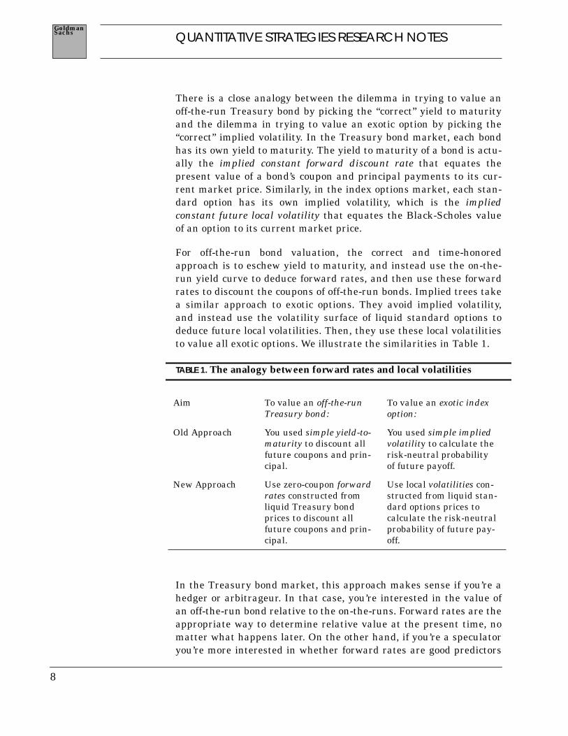
For off-the-run bond valuation, the correct and time-honoredapproach is to eschew yield to maturity, and instead use the on-the-run yield curve to deduce forward rates, and then use these forwardrates to discount the coupons of off-the-run bonds. Implied trees takea similar approach to exotic options. They avoid implied volatility,and instead use the volatility surface of liquid standard options todeduce future local volatilities. Then, they use these local volatilitiesto value all exotic options. We illustrate the similarities in Table 1.

In the Treasury bond market, this approach makes sense if you’re ahedger or arbitrageur. In that case, you’re interested in the value ofan off-the-run bond relative to the on-the-runs. Forward rates are theappropriate way to determine relative value at the present time, nomatter what happens later. On the other hand, if you’re a speculatoryou’re more interested in whether forward rates are good predictors

TABLE 1. The analogy between forward rates and local volatilities

Aim To value an off-the-runTreasury bond:

To value an exotic indexoption:

Old Approach You used simple yield-to-maturity to discount allfuture coupons and prin-cipal.

You used simple impliedvolatility to calculate therisk-neutral probabilityof future payoff.

New Approach Use zero-coupon forwardrates constructed fromliquid Treasury bondprices to discount allfuture coupons and prin-cipal.

Use local volatilities con-structed from liquid stan-dard options prices tocalculate the risk-neutralprobability of future pay-off.

9


of future rates, and arbitrage pricing is less important. Similarly, inthe equity index options market, local volatilities are the appropriateway to determine the value of an exotic option relative to standardoptions, no matter what future levels volatility takes.

You can lock in forward rates by buying a longer-term bond and sell-ing a shorter-term bond so that your net cost is zero. Analogously, youcan lock in forward (local) volatility by buying a calendar spread andselling butterfly spreads with a zero net cost.

10


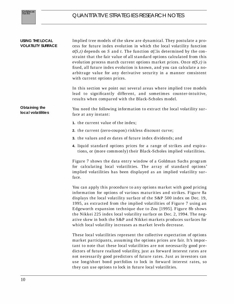
Implied tree models of the skew are dynamical. They postulate a pro-cess for future index evolution in which the local volatility functionσ(S,t) depends on S and t. The function σ() is determined by the con-straint that the fair value of all standard options calculated from thisevolution process match current options market prices. Once σ(S,t) isfixed, all future index evolution is known, and you can calculate a no-arbitrage value for any derivative security in a manner consistentwith current options prices.

In this section we point out several areas where implied tree modelslead to significantly different, and sometimes counter-intuitive,results when compared with the Black-Scholes model.

You need the following information to extract the local volatility sur-face at any instant:

1. the current value of the index;

2. the current (zero-coupon) riskless discount curve;

3. the values and ex dates of future index dividends; and

4. liquid standard options prices for a range of strikes and expira-tions, or (more commonly) their Black-Scholes implied volatilities.

Figure 7 shows the data entry window of a Goldman Sachs programfor calculating local volatilities. The array of standard options’implied volatilities has been displayed as an implied volatility sur-face.

You can apply this procedure to any options market with good pricinginformation for options of various maturities and strikes. Figure 8adisplays the local volatility surface of the S&P 500 index on Dec. 19,1995, as extracted from the implied volatilities of Figure 7 using anEdgeworth expansion technique due to Zou [1995]. Figure 8b showsthe Nikkei 225 index local volatility surface on Dec. 2, 1994. The neg-ative skew in both the S&P and Nikkei markets produces surfaces forwhich local volatility increases as market levels decrease.

These local volatilities represent the collective expectation of optionsmarket participants, assuming the options prices are fair. It’s impor-tant to note that these local volatilities are not necessarily good pre-dictors of future realized volatility, just as forward interest rates arenot necessarily good predictors of future rates. Just as investors canuse long/short bond portfolios to lock in forward interest rates, sothey can use options to lock in future local volatilities.

USING THE LOCALVOLATILITY SURFACE

Obtaining thelocal volatilities

11


FIGURE 7. Inputs to a program for calculating local volatilities. The plotshows the implied volatility surface for the S&P 500 index on October10, 1995. Estimated future dividends of the index are not displayed.

12


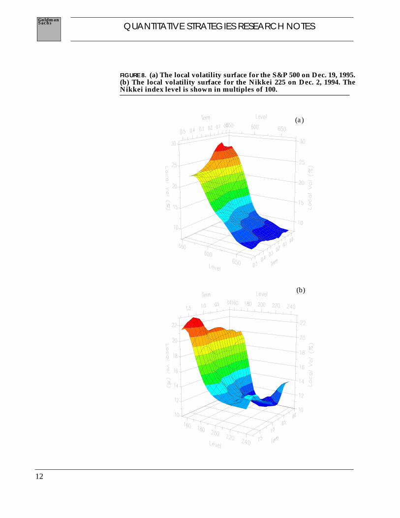
FIGURE 8. (a) The local volatility surface for the S&P 500 on Dec. 19, 1995.(b) The local volatility surface for the Nikkei 225 on Dec. 2, 1994. TheNikkei index level is shown in multiples of 100.

(a)

(b)

13


The local volatility surface indicates the fair value of local volatilityat future times and market levels. The most striking feature of Fig-ure 8 is the systematic decrease of local index volatility with increas-ing index level. This implied correlation between index level andlocal volatility is essentially responsible for all of the qualitative fea-tures of our results below.

The variation in S&P 500 local volatility displayed in Figure 8a isgenerally greater than the variation in implied volatility in Figure 7that produced it. For skewed options markets, we note the followingheuristic rule5:

Figure 9 illustrates this relationship. For theoretical insight, see theAppendix, and also Kani and Kamal [1996].

5. The three rules of thumb that appear below apply to short and intermediate termequity index options, where the correlation between index level and volatility ismost pronounced and the assumption of approximately linear skew seems to begood. For longer term options, other factors, such as stochastic volatility or vola-tility mean reversion, may start to blur the effects of correlation that we haveencapsulated in these three rules.

Rule of Thumb 1: Local volatility varies withmarket level about twice as rapidly as implied vol-atility varies with strike.

The correlationbetween index leveland index volatility

FIGURE 9. In the implied tree model, local volatility varies with indexlevel approximately twice as rapidly as implied volatility varieswith strike level.

volatility

level

implied

local

14


If you can estimate future index dividend yields and growth rates,you can use the local volatility surface to simulate the evolution ofthe index to generate index distributions at any future time. Figure10 shows the end-of-year S&P 500 distributions implied by liquidoptions prices during mid-July 1995, a turbulent time for the U.S.equity market. In generating these distributions we have assumedan expected annual growth rate of 6% and dividend yield of 2.5% peryear.

On Monday, July 17, the S&P 500 index closed at a record high of562.72. On Tuesday, July 18, the Dow Jones Industrials Indexdropped more than 50 points and the S&P closed at 558.46. OnWednesday, July 19, the Dow Jones fell about another 57 points, andthe S&P closed at 550.98. The shift in market sentiment during thesethree days is reflected in the changing shapes of the distributions.For instance, a shoulder at the 550 level materialized on July 18,indicating a more negative view of the market. By July 19, a peak atthe 480 level became apparent.

Investors whose views of future market distributions differ from thatimplied by options prices can take advantage of the differences bybuying or selling options.

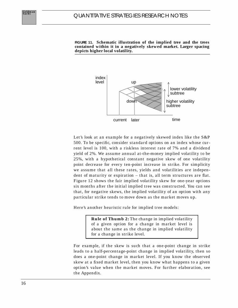
Once fitted to current interest rates, dividend yields and implied vol-atilities, the implied tree model produces a tree of future index levelsand their associated fair local volatility, as implied by options prices.Figure 11 displays a schematic version of the implied tree for a nega-tively skewed market. with its origin at the time labeled current.Assuming the market’s perception of local volatility remainsunchanged as time passes and the index moves, we can use theselocal volatilities to calculate the dependence of implied volatility onstrike at future times. If, at some time labeled later in Figure 11, theindex moves to either of the levels labeled up or down, the evolutionof the index is described by the subtrees labeled up or down. This isvalid provided no new information about future volatility, other thana market level move, has arrived between the time the initial treewas built and the time at which the index has moved to the start of anew subtree.You can use the up or down tree to calculate fair valuesfor options of all strikes and expirations at time later. You can thenconvert these prices into Black-Scholes implied volatilities, and socompute the fair future implied volatility surfaces and skew plots.

Implied distributionsand market sentiment

The future evolution ofthe smile

15


FIGURE 10. Implied S&P 500 distributions on Dec. 31, 1995, based onS&P 500 implied volatilities on July 17, 18 and 19, 1995. We assume agrowth rate of 6% and dividend yield of 2.5% to year end.

Probability (%)

400 45

0

500

550

600

650

700

0.00

3.00

6.00

9.00

12.00

400 45

0

500

550

600

650

700

0.00

3.00

6.00

9.00

12.00

400 45

0

500

550

600

650

700

0.00

3.00

6.00

9.00

12.00

Index Level

7/17/95

S&P close 562.72

7/18/95

S&P close 558.46

7/19/95

S&P close 550.98

16


Let’s look at an example for a negatively skewed index like the S&P500. To be specific, consider standard options on an index whose cur-rent level is 100, with a riskless interest rate of 7% and a dividendyield of 2%. We assume annual at-the-money implied volatility to be25%, with a hypothetical constant negative skew of one volatilitypoint decrease for every ten-point increase in strike. For simplicitywe assume that all these rates, yields and volatilities are indepen-dent of maturity or expiration – that is, all term structures are flat.Figure 12 shows the fair implied volatility skew for one-year optionssix months after the initial implied tree was constructed. You can seethat, for negative skews, the implied volatility of an option with anyparticular strike tends to move down as the market moves up.

Here’s another heuristic rule for implied tree models:

For example, if the skew is such that a one-point change in strikeleads to a half-percentage-point change in implied volatility, then sodoes a one-point change in market level. If you know the observedskew at a fixed market level, then you know what happens to a givenoption’s value when the market moves. For further elaboration, seethe Appendix.

Rule of Thumb 2: The change in implied volatilityof a given option for a change in market level isabout the same as the change in implied volatilityfor a change in strike level.

indexlevel

time

FIGURE 11. Schematic illustration of the implied tree and the treescontained within it in a negatively skewed market. Larger spacingdepicts higher local volatility.

current later

up

down

lower volatilitysubtree

higher volatilitysubtree

17


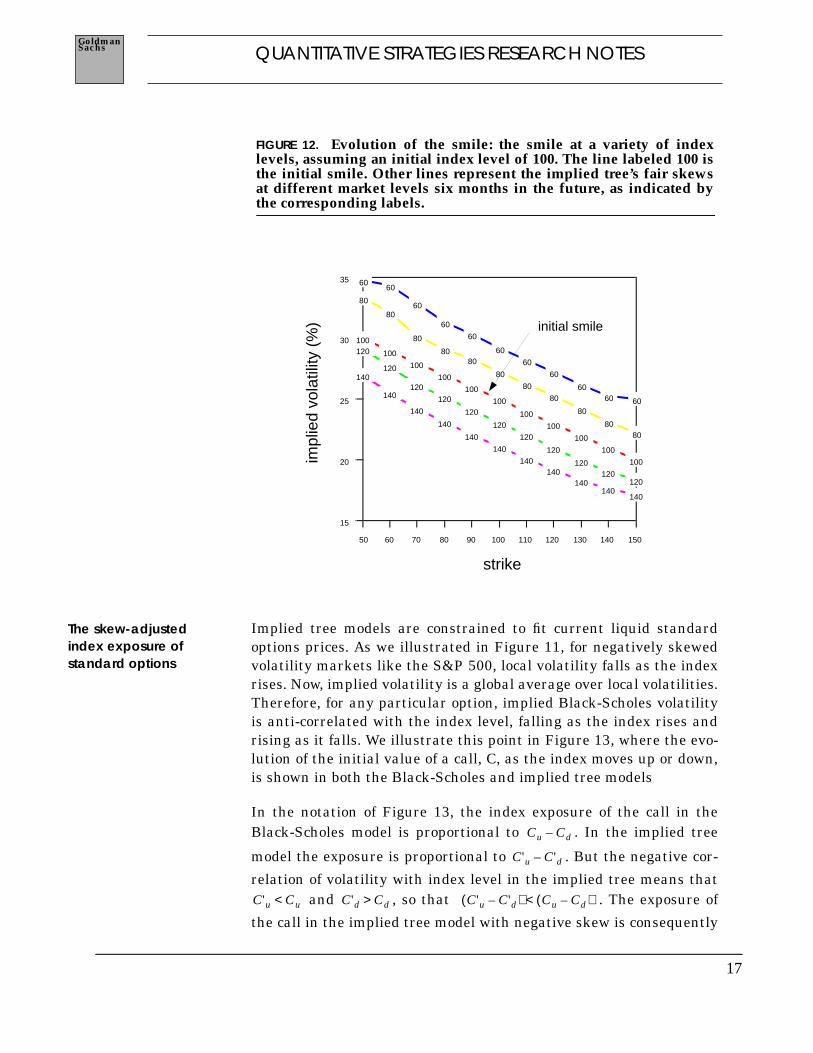
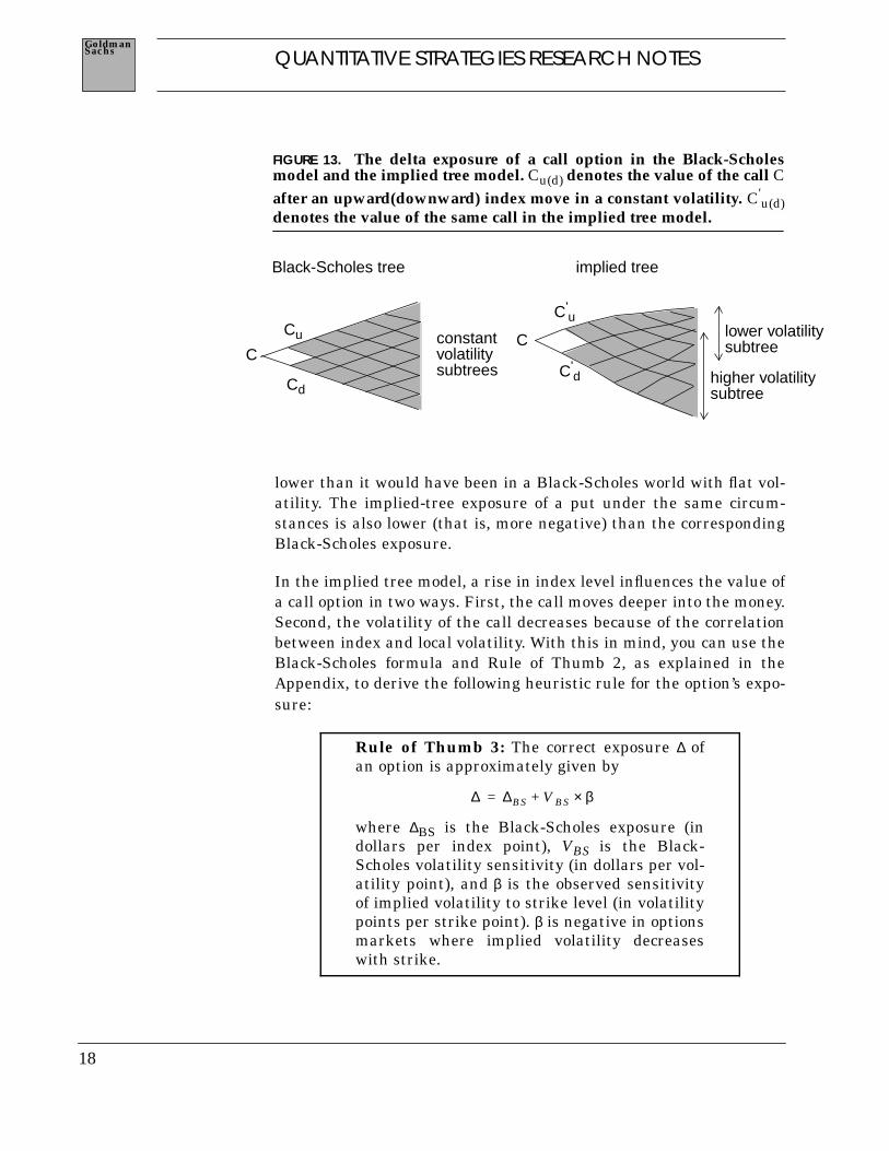
Implied tree models are constrained to fit current liquid standardoptions prices. As we illustrated in Figure 11, for negatively skewedvolatility markets like the S&P 500, local volatility falls as the indexrises. Now, implied volatility is a global average over local volatilities.Therefore, for any particular option, implied Black-Scholes volatilityis anti-correlated with the index level, falling as the index rises andrising as it falls. We illustrate this point in Figure 13, where the evo-lution of the initial value of a call, C, as the index moves up or down,is shown in both the Black-Scholes and implied tree models

In the notation of Figure 13, the index exposure of the call in theBlack-Scholes model is proportional to . In the implied tree

model the exposure is proportional to . But the negative cor-

relation of volatility with index level in the implied tree means that and , so that . The exposure of

the call in the implied tree model with negative skew is consequently

FIGURE 12. Evolution of the smile: the smile at a variety of indexlevels, assuming an initial index level of 100. The line labeled 100 isthe initial smile. Other lines represent the implied tree’s fair skewsat different market levels six months in the future, as indicated bythe corresponding labels.

50 60 70 80 90 100 110 120 130 140 150

15

20

25

30

35

140

140

140

140

140

140

140 140

140 140

140

120

120

120

120

120

120

120

120

120 120

120

80

80

80

80 80

80

80

80

80

80 80

60 60

60

60

60

60

60

60

60 60 60

100

100

100

100

100

100

100

100

100

100

100

strike

impl

ied

vola

tility

(%

) initial smile

The skew-adjustedindex exposure ofstandard options

Cu Cd–

C'u C'd–

C'u Cu< C'd Cd> C'u C'd–( ) Cu Cd–( )<

18


lower than it would have been in a Black-Scholes world with flat vol-atility. The implied-tree exposure of a put under the same circum-stances is also lower (that is, more negative) than the correspondingBlack-Scholes exposure.

In the implied tree model, a rise in index level influences the value ofa call option in two ways. First, the call moves deeper into the money.Second, the volatility of the call decreases because of the correlationbetween index and local volatility. With this in mind, you can use theBlack-Scholes formula and Rule of Thumb 2, as explained in theAppendix, to derive the following heuristic rule for the option’s expo-sure:

Rule of Thumb 3: The correct exposure ∆ ofan option is approximately given by

where ∆BS is the Black-Scholes exposure (indollars per index point), VBS is the Black-Scholes volatility sensitivity (in dollars per vol-atility point), and β is the observed sensitivityof implied volatility to strike level (in volatilitypoints per strike point). β is negative in optionsmarkets where implied volatility decreaseswith strike.

Black-Scholes tree implied tree

FIGURE 13. The delta exposure of a call option in the Black-Scholesmodel and the implied tree model. Cu(d) denotes the value of the call Cafter an upward(downward) index move in a constant volatility. C'

u(d)denotes the value of the same call in the implied tree model.

lower volatilitysubtree

higher volatilitysubtree

constantvolatilitysubtrees

Cu

Cd

C'u

C'd

Black-Scholes tree implied tree

CC

∆ ∆BS V BS β×+=

19


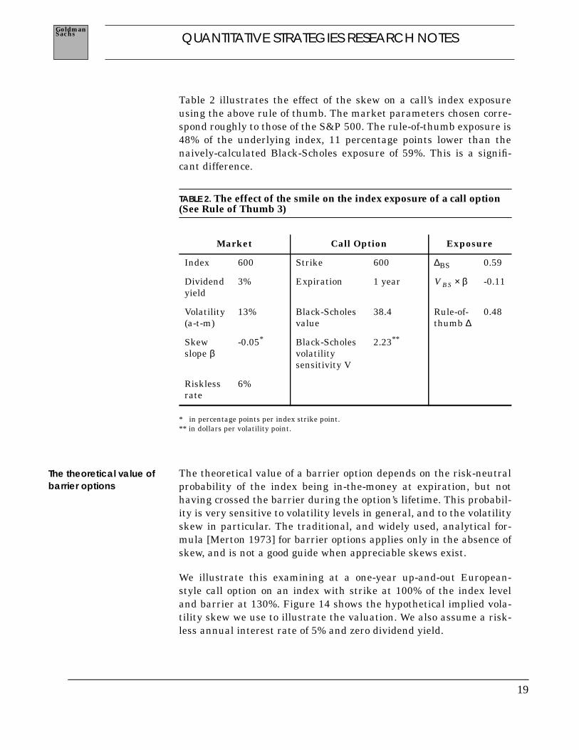
Table 2 illustrates the effect of the skew on a call’s index exposureusing the above rule of thumb. The market parameters chosen corre-spond roughly to those of the S&P 500. The rule-of-thumb exposure is48% of the underlying index, 11 percentage points lower than thenaively-calculated Black-Scholes exposure of 59%. This is a signifi-cant difference.

TABLE 2. The effect of the smile on the index exposure of a call option(See Rule of Thumb 3)

* in percentage points per index strike point.** in dollars per volatility point.

The theoretical value of a barrier option depends on the risk-neutralprobability of the index being in-the-money at expiration, but nothaving crossed the barrier during the option’s lifetime. This probabil-ity is very sensitive to volatility levels in general, and to the volatilityskew in particular. The traditional, and widely used, analytical for-mula [Merton 1973] for barrier options applies only in the absence ofskew, and is not a good guide when appreciable skews exist.

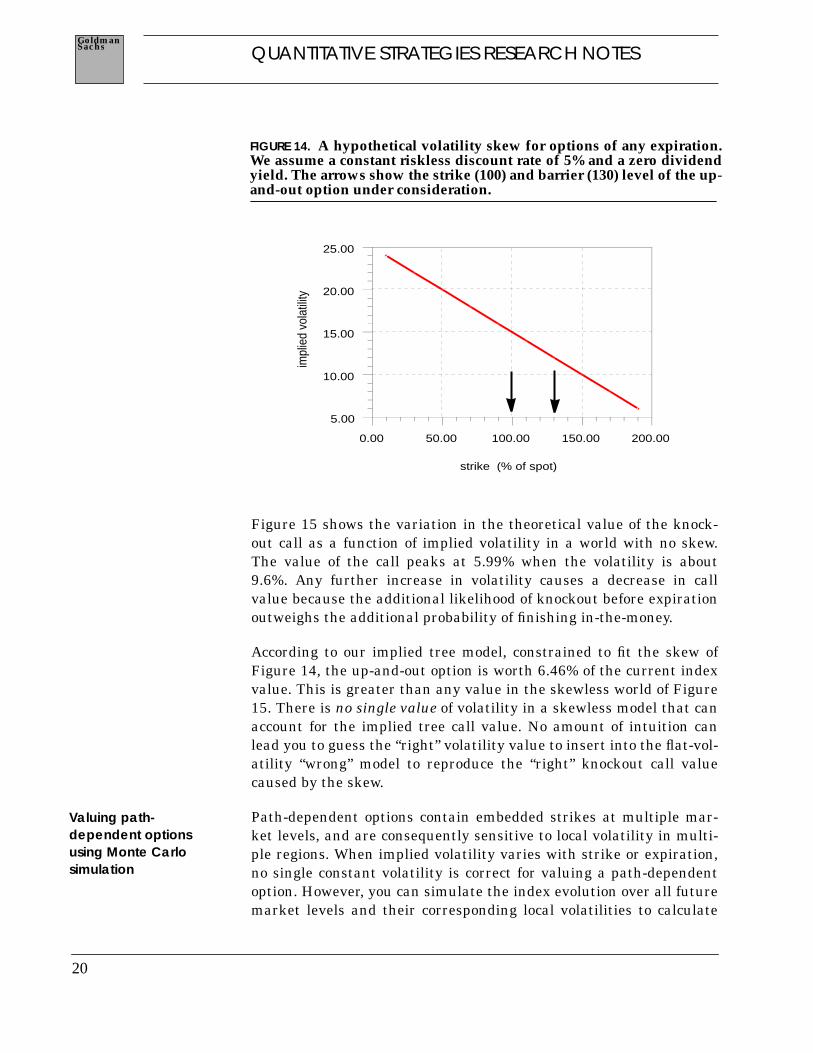
We illustrate this examining at a one-year up-and-out European-style call option on an index with strike at 100% of the index leveland barrier at 130%. Figure 14 shows the hypothetical implied vola-tility skew we use to illustrate the valuation. We also assume a risk-less annual interest rate of 5% and zero dividend yield.

Market Call Option Exposure

Index 600 Strike 600 ∆BS 0.59

Dividendyield

3% Expiration 1 year -0.11

Volatility(a-t-m)

13% Black-Scholesvalue

38.4 Rule-of-thumb ∆

0.48

Skewslope β

-0.05* Black-Scholesvolatilitysensitivity V

2.23**

Risklessrate

6%

V BS β×

The theoretical value ofbarrier options

20


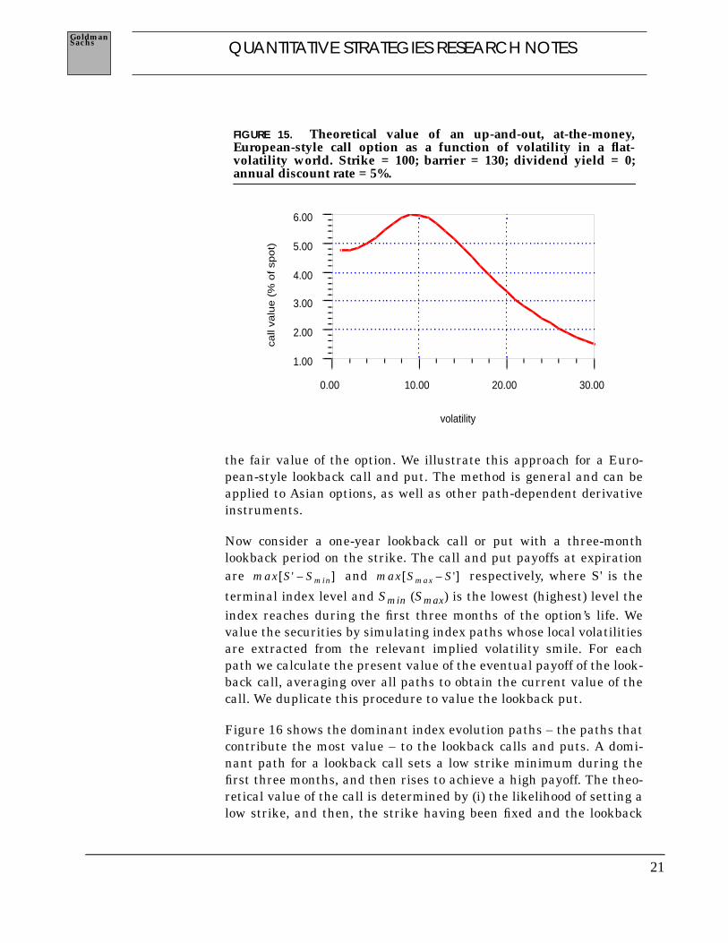
Figure 15 shows the variation in the theoretical value of the knock-out call as a function of implied volatility in a world with no skew.The value of the call peaks at 5.99% when the volatility is about9.6%. Any further increase in volatility causes a decrease in callvalue because the additional likelihood of knockout before expirationoutweighs the additional probability of finishing in-the-money.

According to our implied tree model, constrained to fit the skew ofFigure 14, the up-and-out option is worth 6.46% of the current indexvalue. This is greater than any value in the skewless world of Figure15. There is no single value of volatility in a skewless model that canaccount for the implied tree call value. No amount of intuition canlead you to guess the “right” volatility value to insert into the flat-vol-atility “wrong” model to reproduce the “right” knockout call valuecaused by the skew.

Path-dependent options contain embedded strikes at multiple mar-ket levels, and are consequently sensitive to local volatility in multi-ple regions. When implied volatility varies with strike or expiration,no single constant volatility is correct for valuing a path-dependentoption. However, you can simulate the index evolution over all futuremarket levels and their corresponding local volatilities to calculate

FIGURE 14. A hypothetical volatility skew for options of any expiration.We assume a constant riskless discount rate of 5% and a zero dividendyield. The arrows show the strike (100) and barrier (130) level of the up-and-out option under consideration.

strike (% of spot)

0.00 50.00 100.00 150.00 200.00

impl

ied

vola

tility

5.00

10.00

15.00

20.00

25.00

Valuing path-dependent optionsusing Monte Carlosimulation

21


the fair value of the option. We illustrate this approach for a Euro-pean-style lookback call and put. The method is general and can beapplied to Asian options, as well as other path-dependent derivativeinstruments.

Now consider a one-year lookback call or put with a three-monthlookback period on the strike. The call and put payoffs at expirationare and respectively, where S' is the

terminal index level and Smin (Smax) is the lowest (highest) level theindex reaches during the first three months of the option’s life. Wevalue the securities by simulating index paths whose local volatilitiesare extracted from the relevant implied volatility smile. For eachpath we calculate the present value of the eventual payoff of the look-back call, averaging over all paths to obtain the current value of thecall. We duplicate this procedure to value the lookback put.

Figure 16 shows the dominant index evolution paths – the paths thatcontribute the most value – to the lookback calls and puts. A domi-nant path for a lookback call sets a low strike minimum during thefirst three months, and then rises to achieve a high payoff. The theo-retical value of the call is determined by (i) the likelihood of setting alow strike, and then, the strike having been fixed and the lookback

FIGURE 15. Theoretical value of an up-and-out, at-the-money,European-style call option as a function of volatility in a flat-volatility world. Strike = 100; barrier = 130; dividend yield = 0;annual discount rate = 5%.

call

valu

e (

% o

f sp

ot)

volatility

0.00 10.00 20.00 30.00

1.00

2.00

3.00

4.00

5.00

6.00

max S' Smin–[ ] max Smax S'–[ ]

22


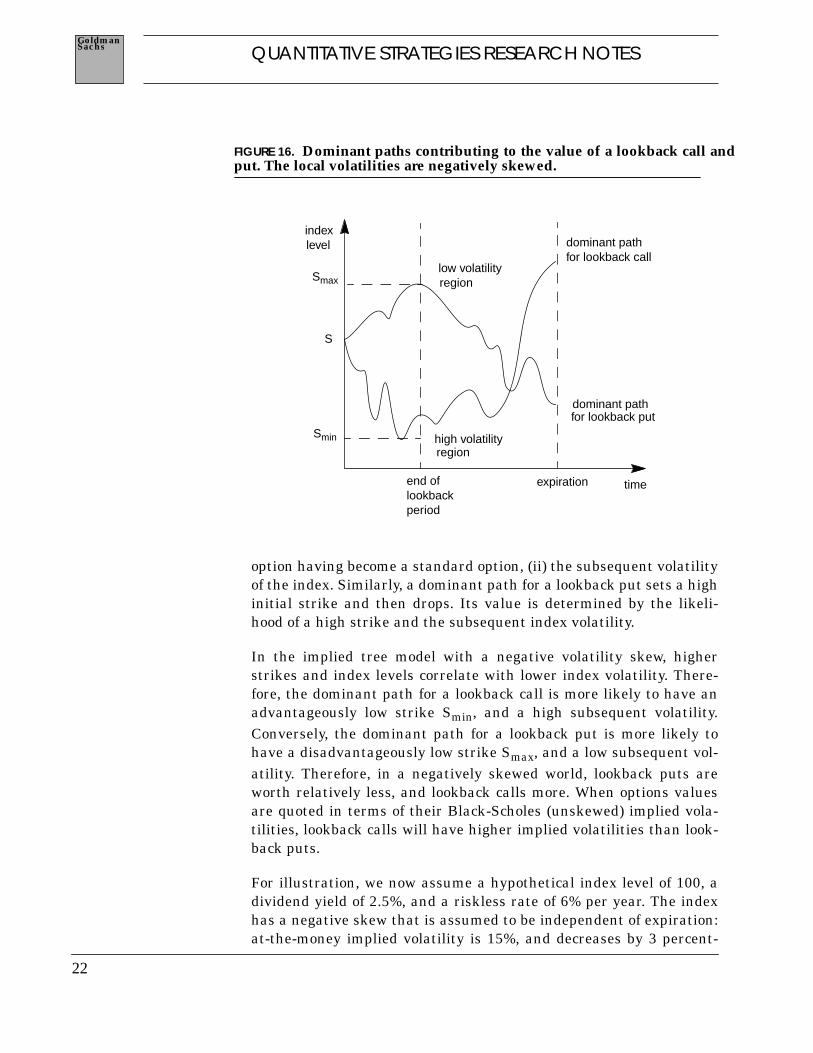
option having become a standard option, (ii) the subsequent volatilityof the index. Similarly, a dominant path for a lookback put sets a highinitial strike and then drops. Its value is determined by the likeli-hood of a high strike and the subsequent index volatility.

In the implied tree model with a negative volatility skew, higherstrikes and index levels correlate with lower index volatility. There-fore, the dominant path for a lookback call is more likely to have anadvantageously low strike Smin, and a high subsequent volatility.Conversely, the dominant path for a lookback put is more likely tohave a disadvantageously low strike Smax, and a low subsequent vol-atility. Therefore, in a negatively skewed world, lookback puts areworth relatively less, and lookback calls more. When options valuesare quoted in terms of their Black-Scholes (unskewed) implied vola-tilities, lookback calls will have higher implied volatilities than look-back puts.

For illustration, we now assume a hypothetical index level of 100, adividend yield of 2.5%, and a riskless rate of 6% per year. The indexhas a negative skew that is assumed to be independent of expiration:at-the-money implied volatility is 15%, and decreases by 3 percent-

FIGURE 16. Dominant paths contributing to the value of a lookback call andput. The local volatilities are negatively skewed.

time

indexlevel

end oflookbackperiod

expiration

S

Smin

Smax

dominant pathfor lookback call

dominant pathfor lookback put

high volatilityregion

low volatilityregion

23


age points for each increase of 10 index strike points. Using MonteCarlo simulation, we find the fair value of the lookback call to be10.8% of the index, and the value of the lookback put to be 5.8%. Inthe framework of an unskewed, Black-Scholes index, these valuescorrespond to an implied volatility of 15.6% for the lookback call and13.0% for the lookback put.

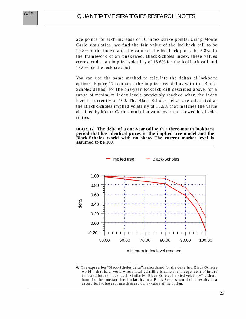
You can use the same method to calculate the deltas of lookbackoptions. Figure 17 compares the implied-tree deltas with the Black-Scholes deltas6 for the one-year lookback call described above, for arange of minimum index levels previously reached when the indexlevel is currently at 100. The Black-Scholes deltas are calculated atthe Black-Scholes implied volatility of 15.6% that matches the valueobtained by Monte Carlo simulation value over the skewed local vola-tilities.

6. The expression “Black-Scholes delta” is shorthand for the delta in a Black-Scholesworld – that is, a world where local volatility is constant, independent of futuretime and future index level. Similarly, “Black-Scholes implied volatility” is short-hand for the constant local volatility in a Black-Scholes world that results in atheoretical value that matches the dollar value of the option.

implied tree Black-Scholes

minimum index level reached

50.00 60.00 70.00 80.00 90.00 100.00

delta

-0.20

0.00

0.20

0.40

0.60

0.80

1.00

FIGURE 17. The delta of a one-year call with a three-month lookbackperiod that has identical prices in the implied tree model and theBlack-Scholes world with no skew. The current market level isassumed to be 100.

24


Note that the delta of the lookback call is always lower in the impliedtree model than in the Black-Scholes model. This mismatch in modeldeltas occurs because, in the implied tree model, the option’s sensitiv-ity to volatility also contributes to its index exposure through the cor-relation between volatility and index level (see Rule of Thumb 3). Themismatch is greatest where volatility sensitivity is largest, that is,where the minimum index level is close to the current index level.The mismatch is correspondingly smallest when the lowest level pre-viously reached is much lower than the current index level, since thelookback is effectively a forward contract with zero volatility sensitiv-ity. The fact that the theoretical delta of an at-the-money lookbackcall is negative – to hedge a long call position you must actually golong the index – is initially quite astonishing to market participants.

A similar effect holds for lookback puts, whose implied-tree deltas arealso always numerically lower (that is, negative and larger in magni-tude) than the corresponding Black-Scholes deltas.

25


In this appendix we provide some insight into our three rules ofthumb. Our treatment is intuitive; for a more rigorous approach seeKani and Kamal [1996].

We restrict ourselves to the simple case in which the value of localvolatility for an index is independent of future time, and varies lin-early with index level, so that

(A 1)

If you refer to the variation in future at-the-money local volatility asthe “forward” volatility curve, then you can call this variation withindex level the “sideways” volatility curve.

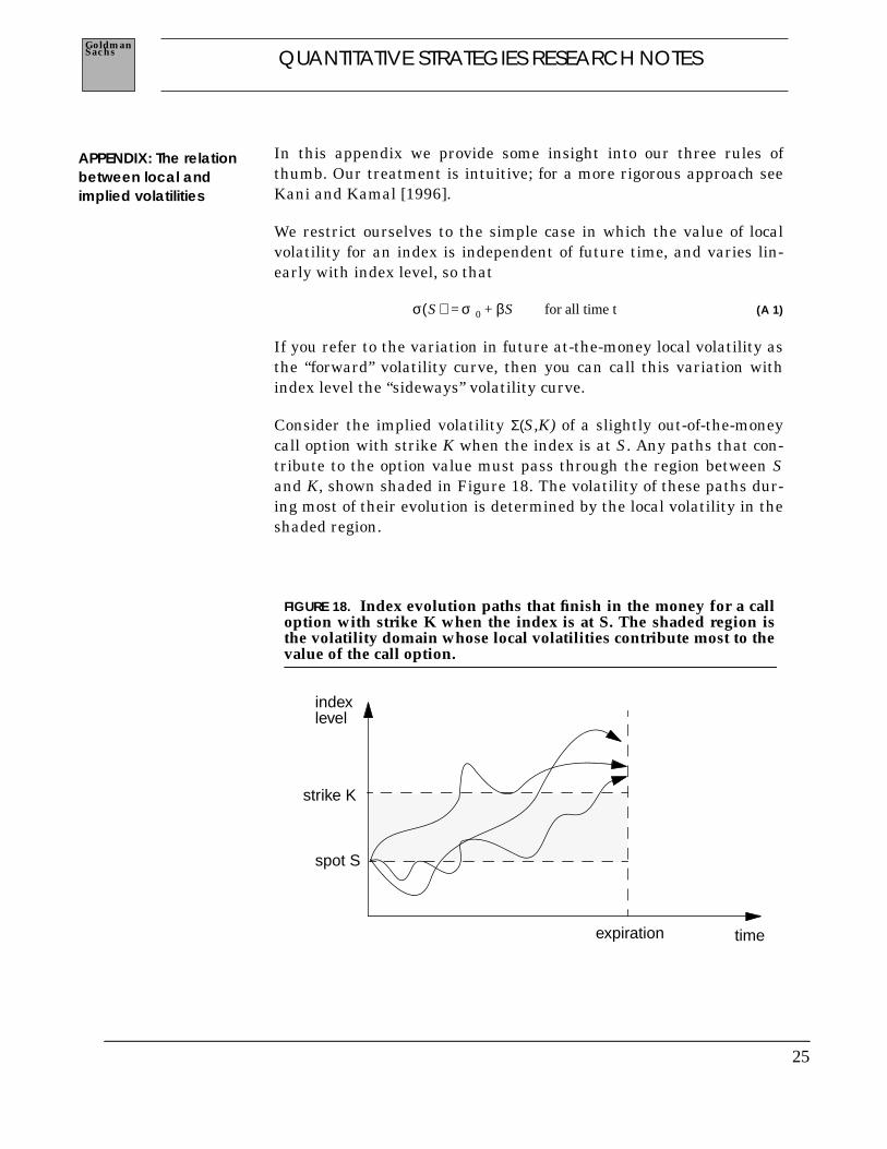
Consider the implied volatility Σ(S,K) of a slightly out-of-the-moneycall option with strike K when the index is at S. Any paths that con-tribute to the option value must pass through the region between Sand K, shown shaded in Figure 18. The volatility of these paths dur-ing most of their evolution is determined by the local volatility in theshaded region.

APPENDIX: The relationbetween local andimplied volatilities

σ S( ) σ0 βS for all time t+=

FIGURE 18. Index evolution paths that finish in the money for a calloption with strike K when the index is at S. The shaded region isthe volatility domain whose local volatilities contribute most to thevalue of the call option.

indexlevel

time

spot S

strike K

expiration

26


Because of this, you can roughly think of the implied volatility for theoption of strike K when the index is at S as the average of the localvolatilities over the shaded region, so that

(A 2)

By substituting Equation A1 into Equation A2 you can show that

(A 3)

Equation A3 shows that, if implied volatility varies linearly withstrike K at a fixed market level S, then it also varies linearly at thesame rate with the index level S itself. This is Rule of Thumb 2 onpage 16. Equation A1 then shows that local volatility varies with S attwice that rate, which is Rule of Thumb 1 on page 13. You can alsocombine Equation A1 and Equation A3 to write the relationshipbetween implied and local volatility more directly as

(A 4)

If represents the Black-Scholes formula for the

value of a call option in the presence of an implied volatility surface, then its exposure is given by

(A 5)

We have used the fact that , a consequence of Equation A3, in

writing the last identity. Equation A5 is equivalent to Rule of Thumb3 on page 18.

Σ S K,( ) 1K S–--------------- σ S'( ) S'd

S

K

∫≈

Σ S K,( ) σ0β2--- S K+( )+≈

Σ S K,( ) σ S( ) β2--- K S–( )+≈

CBS S Σ S K,( ) r t K, , , ,( )

Σ S K,( )

∆Sd

dCBS

S∂∂CBS

Σ∂∂CBS

S∂∂Σ⋅+= =

S∂∂CBS

Σ∂∂CBS

K∂∂Σ⋅+≈

S∂∂Σ

K∂∂Σ≈

27


REFERENCES

Black, F and M. Scholes (1973). The Pricing of Options and CorporateLiabilities. J. Political Economy, 81, 637-59.

Derman, E. and I. Kani (1994). Riding On A Smile, RISK, 7 (Febru-ary), 32-39.

Dupire, B. (1994). Pricing With A Smile, RISK, 7 (January), 18-20.

Kani, I and M. Kamal (1996). Goldman Sachs Quantitative StrategiesResearch Notes, forthcoming.

Merton, R.C. (1973). Theory of Rational Option Pricing, Bell Journalof Economics and Management Science, 4 (Spring), 141-183.

Rubinstein, M. (1994). Implied Binomial Trees, The Journal ofFinance, 49 (July), 771-818.

Zou, J. (1995). Goldman Sachs internal notes, unpublished.

28


SELECTED QUANTITATIVE STRATEGIES PUBLICATIONS

June 1990 Understanding Guaranteed Exchange-Rate ContractsIn Foreign Stock InvestmentsEmanuel Derman, Piotr Karasinskiand Jeffrey S. Wecker

January 1992 Valuing and Hedging Outperformance OptionsEmanuel Derman

March 1992 Pay-On-Exercise OptionsEmanuel Derman and Iraj Kani

June 1993 The Ins and Outs of Barrier OptionsEmanuel Derman and Iraj Kani

January 1994 The Volatility Smile and Its Implied TreeEmanuel Derman and Iraj Kani

May 1994 Static Options ReplicationEmanuel Derman, Deniz Ergenerand Iraj Kani

May 1995 Enhanced Numerical Methods for Optionswith BarriersEmanuel Derman, Iraj Kani, Deniz Ergenerand Indrajit Bardhan

Documents

Quantitative Strategies Research Notes