Quantitative Methods 2

Lecture 3

The Simple Linear

Regression Model

Edmund Malesky, Ph.D., UCSD

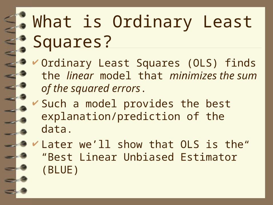
What is Ordinary Least Squares?

Ordinary Least Squares (OLS) finds the linear model that minimizes the sum of the squared errors.

Such a model provides the best explanation/prediction of the data.

Later we’ll show that OLS is the “Best Linear Unbiased Estimator” (BLUE)

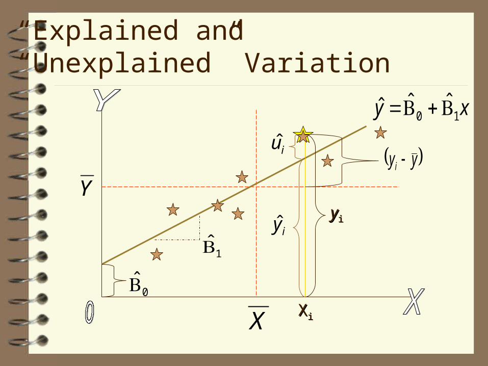
“Explained and “Unexplained” Variation

Y

X

XXii

yyii

0

1

xy 10ˆˆˆ

iy

iu yyi

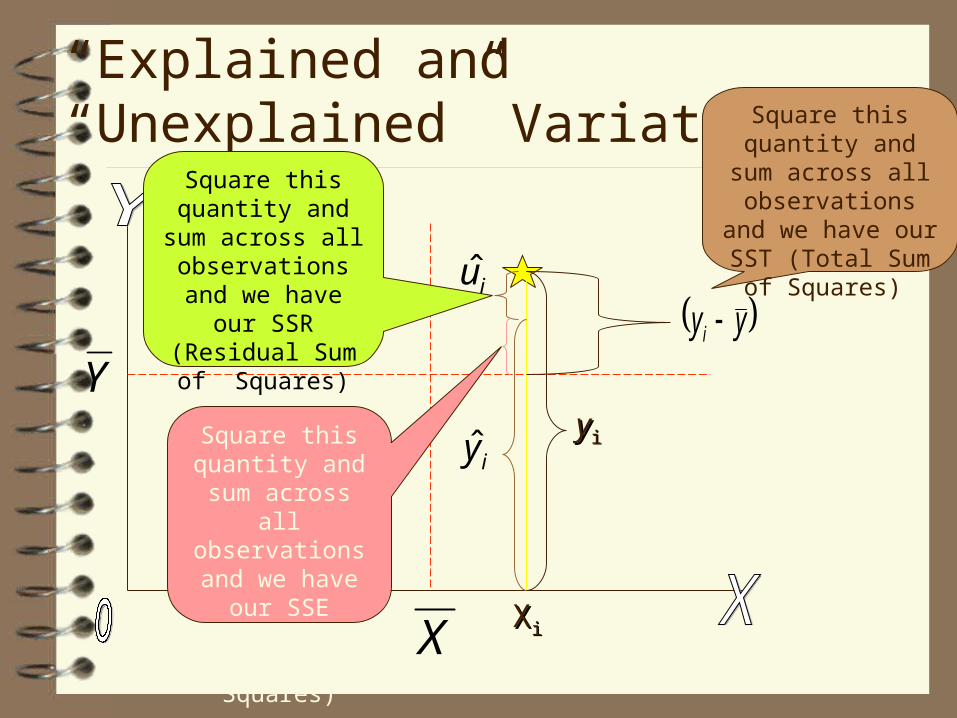
“Explained and “Unexplained” Variation

Y

XXii

yyiiiy

iu yyi

Square this quantity and sum across all observations and we have our SST

(Total Sum of Squares)

Square this quantity and sum

across all observations and we have our SSE (Explained Sum

of Squares)

X

Square this quantity and sum

across all observations and we have our SSR (Residual Sum of

Squares)

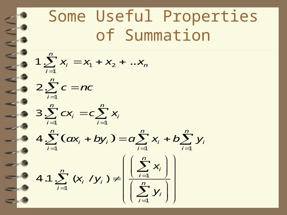
Some Useful Properties of Summation

1 21

1

1 1

1 1 1

1

1

1

1. ...

2.

3.

4.

4.1. ( / )

n

i ni

n

i

n n

i ii i

n n n

i i i ii i i

n

ini

i i ni

ii

x x x x

c nc

cx c x

ax by a x b y

x

x y

y

Some Useful Properties of Summation

Proofs of 7 and 8 in Appendix A of

Wooldridge1 1

1

2 2 2

1 1

1 1 1 1

5. ...and...

6. ( ) 0

7. ( ) ( )

8. ( )( ) ( ) ( ) ( * )

n n

i ii i

n

ii

n n

i ii i

n n n n

i i i i i i i ii i i i

y xy x

n n

x x

x x x n x

x x y y x y y x x y x y n x y

Minimizing the Sum of Squared Errors How to put the Least in OLS? In mathematical jargon we seek to minimize

the residual sum of squares (SSR), where:

n

iii yySSR

1

2ˆ

n

iiu

1

2ˆ

Picking the Parameters

To Minimize SSR, we need parameter estimates.

In calculus, if you wish to know when a function is at its minimum, you take the first derivative.

In this case we must take partial derivatives since we have two parameters (β0 & β1) to worry about.

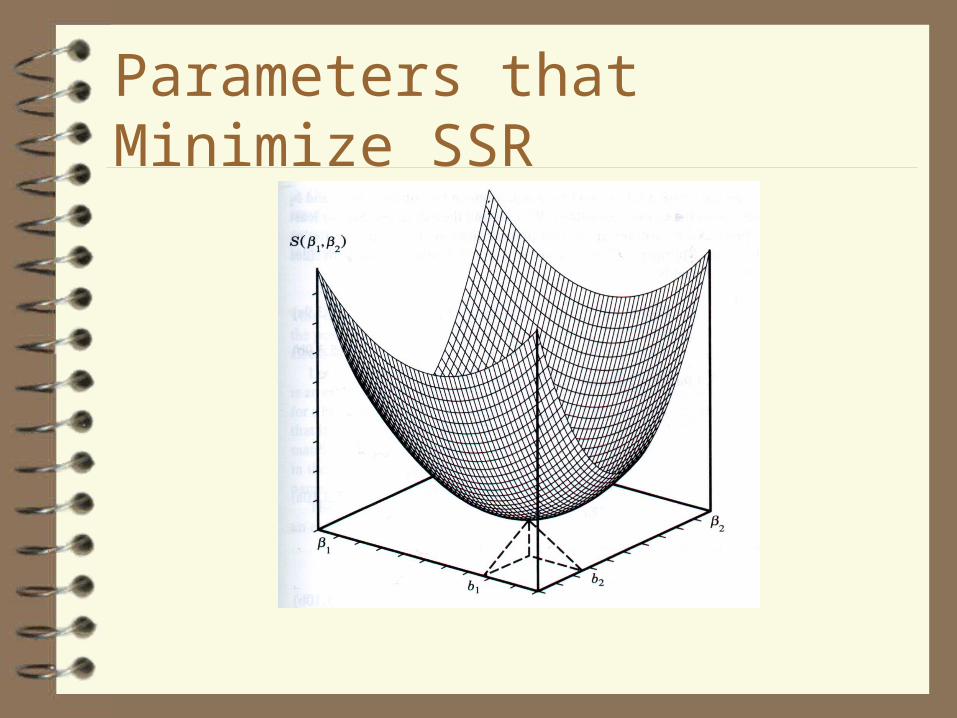
Parameters that Minimize SSR

Minimize the Squared Errors

The SSR Function is:

2ˆ( )i iSSR y y

n

i

uSSR1

2ˆ

20 1( )i iSSR y x

Substitute in our equation

for yhat.

Here comes the magic, Baby!

Simplify TermsPartial Derivative with respect to β0

Partial Derivative with respect to β1

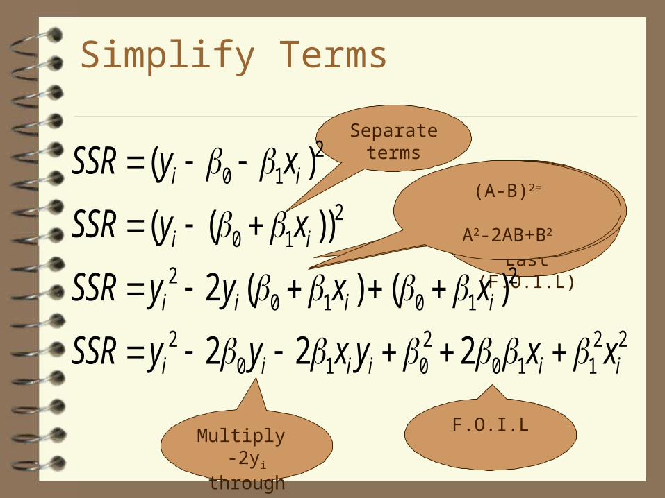
Simplify Terms

Separate terms

First, Outside,

Inside, Last (F.O.I.L)

20 1

20 1

2 20 1 0 1

2 2 2 20 1 0 0 1 1

( )

( ( ))

2 ( ) ( )

2 2 2

i i

i i

i i i i

i i i i i i

SSR y x

SSR y x

SSR y y x x

SSR y y x y x x

Multiply -2yi

through

F.O.I.L

(A-B)2=

A2-BA-AB+B2

(A-B)2=

A2-2AB+B2

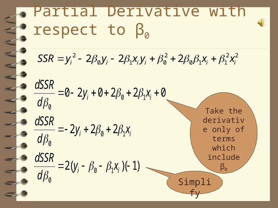
Partial Derivative with respect to β0

2 2 2 20 1 0 0 1 12 2 2i i i i i iSSR y y x y x x

0 10

0 10

0 10

0 2 0 2 2 0

2 2 2

2( )( 1)

i i

i i

i i

dSSRy x

d

dSSRy x

d

dSSRy x

d

Take the derivative

only of terms which

include β0

Simplify

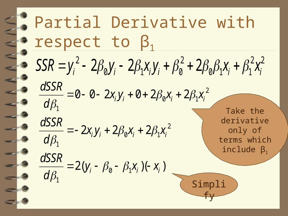
Partial Derivative with respect to β1

20 1

1

20 1

1

0 11

0 0 2 0 2 2

2 2 2

2( )( )

i i i i

i i i i

i i i

dSSRx y x x

d

dSSRx y x x

d

dSSRy x x

d

2 2 2 20 1 0 0 1 12 2 2i i i i i iSSR y y x y x x

Take the derivative

only of terms which include

β1

Simplify

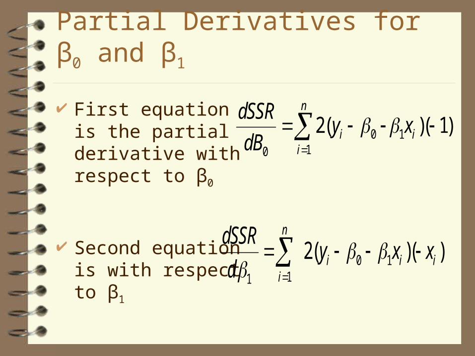
Partial Derivatives for β0 and β1

First equation is the partial derivative with respect to β0

Second equation is with respect to β1 0 1

11

2( )( )n

i i ii

dSSRy x x

d

0 110

2( )( 1)n

i ii

dSSRy x

dB

Simplify and Set Equal to Zero First equation is for β0, second is for β1

Set = 0 to find minimum point (Hats denote that parameters are estimates)

0 10

0 11

ˆ ˆ2 ( ) 0

ˆ ˆ2 ( ) 0

i i

i i i

dSSRy x

dB

dSSRx y x

d

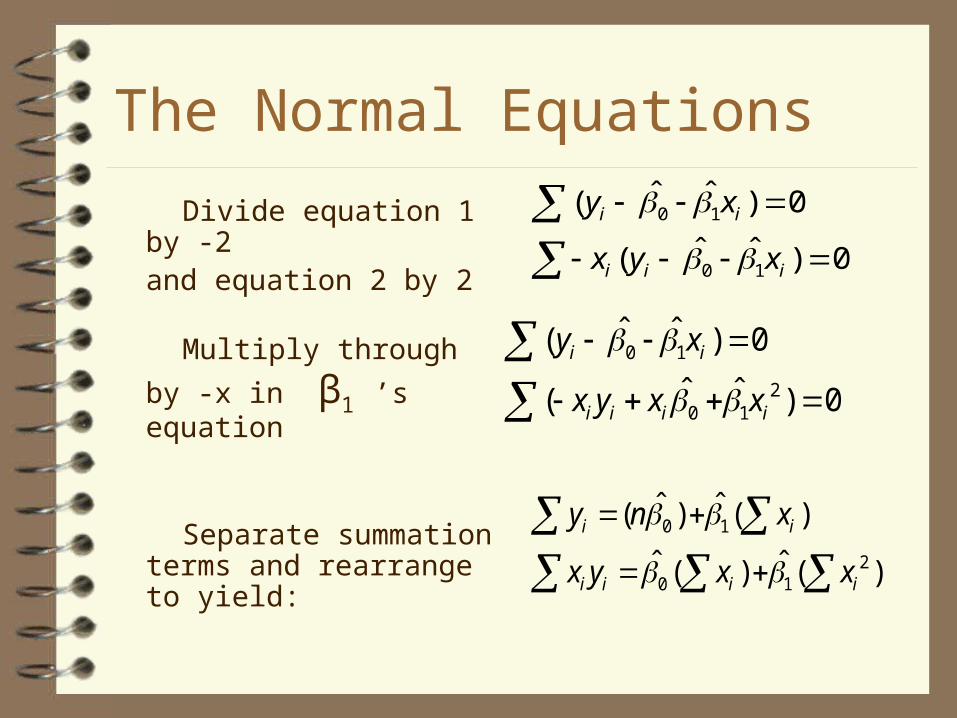
The Normal Equations

Divide equation 1 by -2and equation 2 by 2

Multiply through by -x in

β1 ’s equation

Separate summation terms and rearrange to yield:

0 1

0 1

ˆ ˆ( ) 0

ˆ ˆ( ) 0

i i

i i i

y x

x y x

0 1

20 1

ˆ ˆ( ) 0

ˆ ˆ( ) 0

i i

i i i i

y x

x y x x

0 1

20 1

ˆ ˆ( ) ( )

ˆ ˆ( ) ( )

i i

i i i i

y n x

x y x x

Solving the Normal Equations

Now we have two equations with two unknown terms: β0 and β1

These can be solved using algebra to calculate the values of both β0 and β1

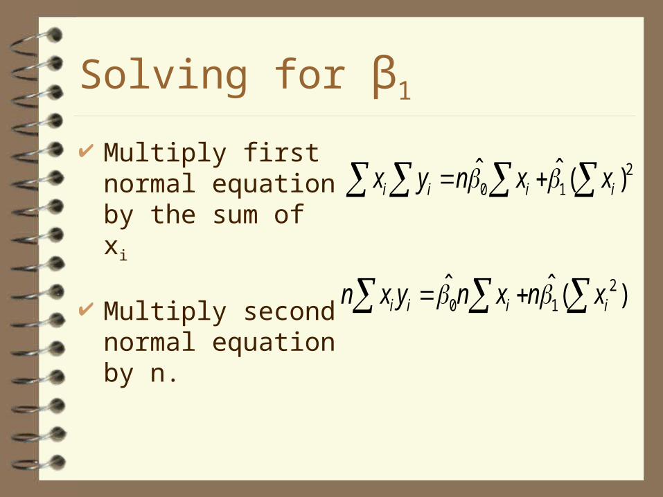
Solving for β1

Multiply first normal equation by the sum of xi

Multiply second normal equation by n.

20 1

ˆ ˆ ( )i i i ix y n x x

20 1

ˆ ˆ ( )i i i in x y n x n x

Still Solving for β1 … Now subtract first equation from the second This yields:

2 20 1 0 1

ˆ ˆ ˆ ˆ( ) ( )

i i i i

i i i i

n x y x y

n x n x n x x

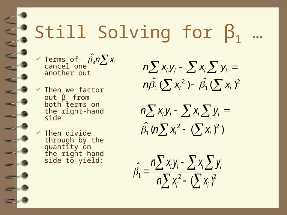
Still Solving for β1 …

2 21 1

ˆ ˆ( ) ( )

i i i i

i i

n x y x y

n x x

0ˆ

in x

2 21( ( ) )

i i i i

i i

n x y x y

n x x

Terms of cancel one another out

Then we factor out β1 from both terms on the right-hand side

Then divide through by the quantity on the right hand side to yield:

1 2 2ˆ

( )i i i i

i i

n x y x y

n x x

A Solution for β1 Now multiply

numerator & denominator by 1/n

Recall that:

This yields:

1 2

( )( )ˆ( )

i i

i

x x y y

x x

...and...i iy xy x

n n

1 22 2

ˆ( )

i ii i i i

i i

i i ii i

x yx y x y nx y n nnx x x

x x nn n n

1 2 2 2

( )( ) ( * )ˆ( )( ) ( )

i i i i

i i

x y n x y x y n x y

x n x x x n x

Tricky: Multiply both sides by1/n*1=1/n*n/n=n/n2

Why?I need to multiply three

separate numbers. I can’t simply split the 1/n.

Imagine I wanted to multiply½(5*10)=25. I can’t solve it

by multiplying 1/2(5)*1/2(10), which equals 12.5. That is like

multiplying by ¼. I need to multiply by ½*1=1/2*2/2=2/4.

Now, 2(1/2*5)(1/2*10)=25

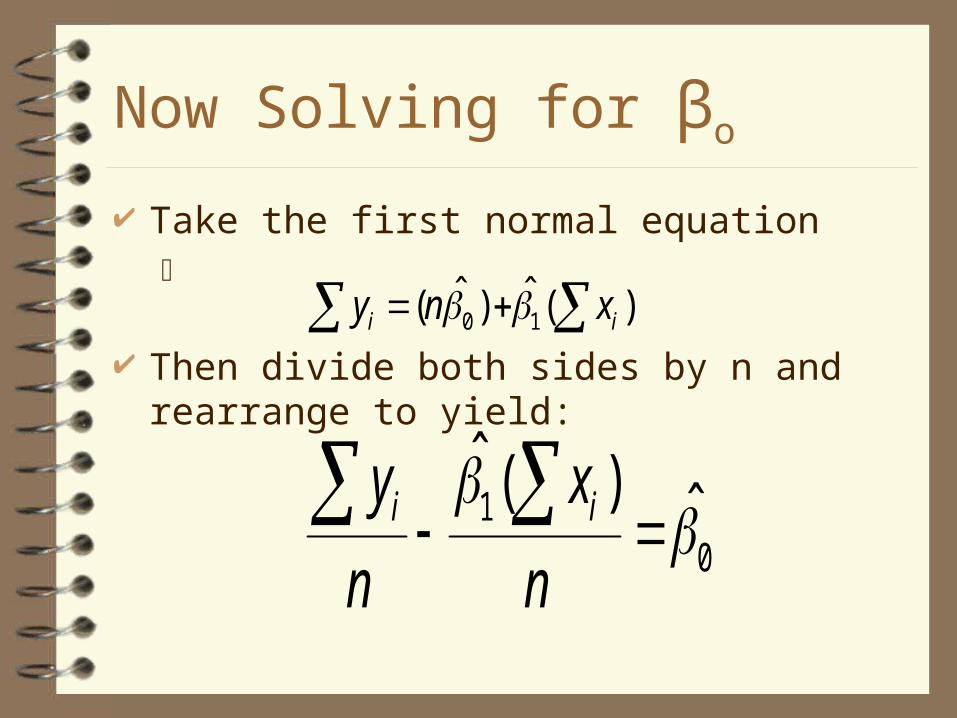
Now Solving for βo

Take the first normal equation

Then divide both sides by n and rearrange to yield:

0 1ˆ ˆ( ) ( )i iy n x

10

ˆ ( ) ˆi iy x

n n

A Solution for βo

Now again that recall that:

Thus:

0 1ˆ ˆy x

...and...i iy xy x

n n

But What Does It Mean?

Equation for β1 may not seem to make

intuitive sense at first But if we break it down into pieces, we can

begin to see the logic

1 2

( )( )ˆ( )

i i

i

x x y y

x x

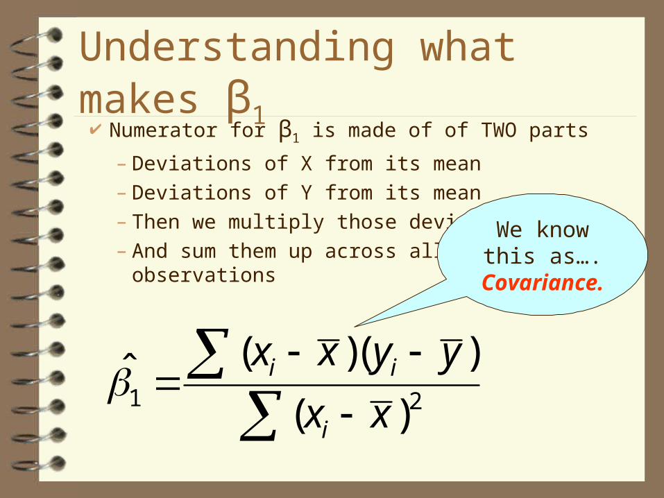
Understanding what makes β1 Numerator for β1 is made of of TWO parts

– Deviations of X from its mean– Deviations of Y from its mean– Then we multiply those deviations– And sum them up across all observations

1 2

( )( )ˆ( )

i i

i

x x y y

x x

We know this as….

Covariance.

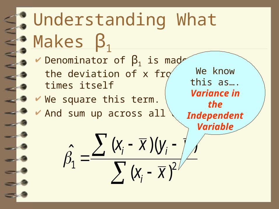
Understanding What Makes β1

Denominator of β1 is made up of the

deviation of x from its mean times itself We square this term. And sum up across all observations

1 2

( )( )ˆ( )

i i

i

x x y y

x x

We know this as….

Variance in the

Independent Variable

Understanding What Makes β1

Thus β1 is made of of changes in x times changes in

y, divided by changes in x squared – A.K.A “rise over run”

Notice if the changes in x are EQUAL to the changes in y, then β1 = 1

1 2

( )( )ˆ( )

i i

i

x x y y

x x

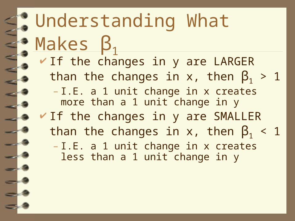
Understanding What Makes β1

If the changes in y are LARGER than the changes in x, then β1 > 1– I.E. a 1 unit change in x creates more than a 1

unit change in y If the changes in y are SMALLER than the

changes in x, then β1 < 1– I.E. a 1 unit change in x creates less than a 1

unit change in y

Understanding What Makes β1

This corresponds to our intuitive understanding of the slope of a line– How much change in y do we observe for each

change in x?

We can also see how β1 is calculated in

units of the dependent variable. – It is changes in the dependent variable over

changes in the independent variable

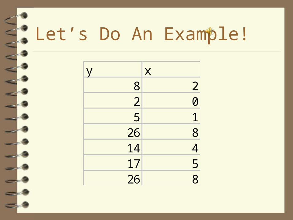
Let’s Do An Example!

y x8 22 05 1

26 814 417 526 8

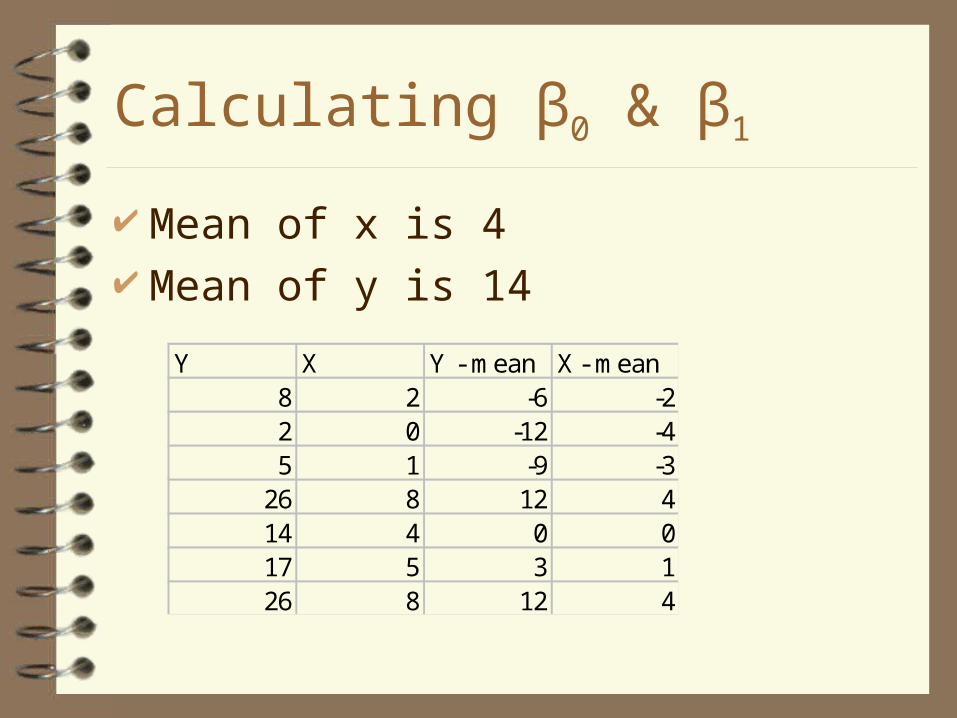
Calculating β0 & β1

Mean of x is 4 Mean of y is 14

Y X Y - mean X - mean8 2 -6 -22 0 -12 -45 1 -9 -3

26 8 12 414 4 0 017 5 3 126 8 12 4

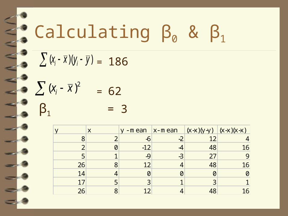
Calculating β0 & β1

= 186

= 62

β1 = 3

( )( )i ix x y y

y x y - mean x- mean (x-x)(y-y) (x-x)(x-x)8 2 -6 -2 12 42 0 -12 -4 48 165 1 -9 -3 27 9

26 8 12 4 48 1614 4 0 0 0 017 5 3 1 3 126 8 12 4 48 16

2( )ix x

Calculating βo and β1

βo = mean of y - β1 (mean of x) Recall that:

– mean of y = 14 & mean of x = 4

βo = 14 - 3(4) βo = 2 Our equation is: y = 2 + 3x

0 1ˆ ˆy x

Which Looks Like…This!

Regression of y on x

0

5

10

15

20

25

30

0 1 2 3 4 5 6 7 8 9

Calculating R2

Let’s return to SSR

Plug in βo and

solve to get

2 20 1

ˆ ˆˆ ( )i i iu y x

2 2 2 21 ˆ( ) ( )i i iy y x x u

SST SSE SSR

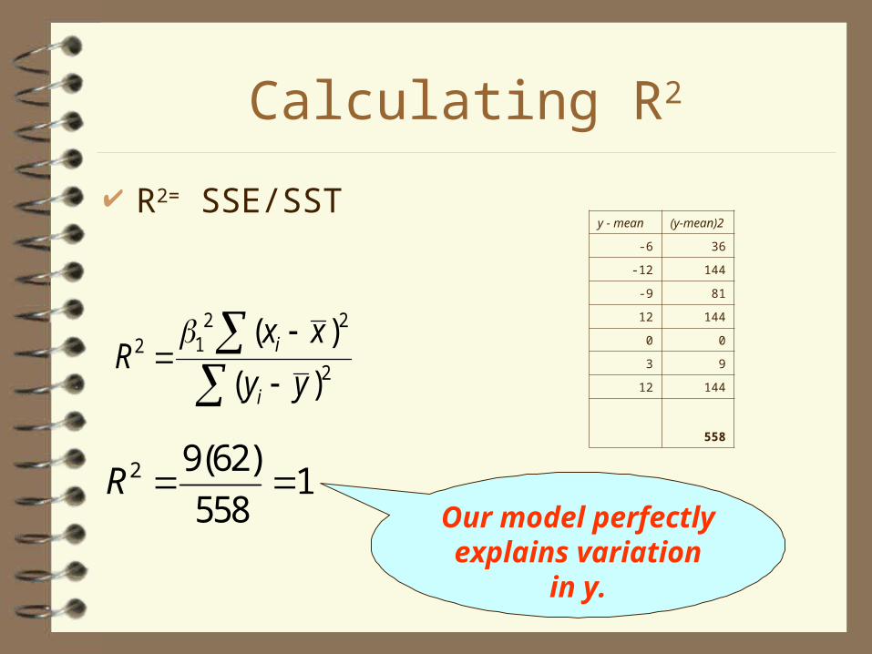
Calculating R2

R2= SSE/SST

2 212

2

( )

( )i

i

x xR

y y

2 9(62)

1558

R

y - mean (y-mean)2

-6 36

-12 144

-9 81

12 144

0 0

3 9

12 144

558

Our model perfectly explains

variation in y.