Embed Size (px)
Citation preview
QUANTITATIVE FINANCEPART II - PORTFOLIO CHOICE
Dr. Luo, Dan
May 30, 2020
Setup Mean-Variance Analysis Unconstrained Optimization Constrained Optimization Back to Portfolio Choice
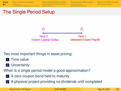
The Single Period Setup
Time 0 Time 1Known Capital Outlay Unknown Future Payoff
Two most important things in asset pricing:1 Time value2 Uncertainty
When is a single period model a good approximation?1 A zero coupon bond held to maturity2 A physical project providing no dividends until completed
QUANTITATIVE FINANCE SoF, SHUFE May 30, 2020 1 / 85
Setup Mean-Variance Analysis Unconstrained Optimization Constrained Optimization Back to Portfolio Choice
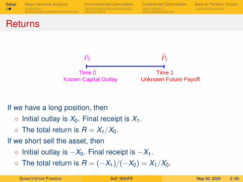
Returns
Time 0 Time 1Known Capital Outlay Unknown Future Payoff
If we have a long position, then� Initial outlay is X0. Final receipt is X1.� The total return is R = X1/X0.
If we short sell the asset, then� Initial outlay is −X0. Final receipt is −X1.� The total return is R = (−X1)/(−X0) = X1/X0.
QUANTITATIVE FINANCE SoF, SHUFE May 30, 2020 2 / 85
Setup Mean-Variance Analysis Unconstrained Optimization Constrained Optimization Back to Portfolio Choice
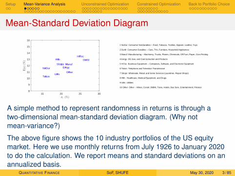
Mean-Standard Deviation Diagram
15 20 25 308
9
10
11
12
13
14
15
16
NoDur
Durbl
ManufEnrgy
HiTec
Telcm
Shops
Hlth
UtilsOther
1 NoDur Consumer Nondurables -- Food, Tobacco, Textiles, Apparel, Leather, Toys
2 Durbl Consumer Durables -- Cars, TVs, Furniture, Household Appliances
3 Manuf Manufacturing -- Machinery, Trucks, Planes, Chemicals, Off Furn, Paper, Com Printing
4 Enrgy Oil, Gas, and Coal Extraction and Products
5 HiTec Business Equipment -- Computers, Software, and Electronic Equipment
6 Telcm Telephone and Television Transmission
7 Shops Wholesale, Retail, and Some Services (Laundries, Repair Shops)
8 Hlth Healthcare, Medical Equipment, and Drugs
9 Utils Utilities
10 Other Other -- Mines, Constr, BldMt, Trans, Hotels, Bus Serv, Entertainment, Finance
A simple method to represent randomness in returns is through atwo-dimensional mean-standard deviation diagram. (Why notmean-variance?)
The above figure shows the 10 industry portfolios of the US equitymarket. Here we use monthly returns from July 1926 to January 2020to do the calculation. We report means and standard deviations on anannualized basis.
QUANTITATIVE FINANCE SoF, SHUFE May 30, 2020 3 / 85
Setup Mean-Variance Analysis Unconstrained Optimization Constrained Optimization Back to Portfolio Choice
Recap
We invest a total amount of X0 in N assets, with amount X0i for asset i ,i = 1,2, ...,N. Let wi = X0i/X0 be the weight of asset i . Obviously,∑N
i=1 wi = 1.
The, the portfolio return is
Rp =
∑Ni=1 RiwiX0
X0=
N∑i=1
wiRi .
Equivalently,
rp =N∑
i=1
wi ri , (1)
because∑N
i=1 wi = 1.
QUANTITATIVE FINANCE SoF, SHUFE May 30, 2020 4 / 85
Setup Mean-Variance Analysis Unconstrained Optimization Constrained Optimization Back to Portfolio Choice
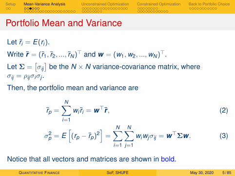
Portfolio Mean and Variance
Let ri = E(ri).
Write r = (r1, r2, ..., rN)> and w = (w1,w2, ...,wN)>.
Let Σ =[σij]
be the N × N variance-covariance matrix, whereσij = ρijσiσj .
Then, the portfolio mean and variance are
rp =N∑
i=1
wi ri = w>r , (2)
σ2p = E
[(rp − rp)2
]=
N∑i=1
N∑j=1
wiwjσij = w>Σw . (3)
Notice that all vectors and matrices are shown in bold.
QUANTITATIVE FINANCE SoF, SHUFE May 30, 2020 5 / 85
Setup Mean-Variance Analysis Unconstrained Optimization Constrained Optimization Back to Portfolio Choice
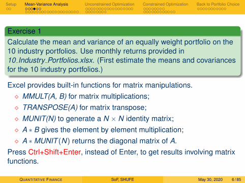
Exercise 1Calculate the mean and variance of an equally weight portfolio on the10 industry portfolios. Use monthly returns provided in10 Industry Portfolios.xlsx. (First estimate the means and covariancesfor the 10 industry portfolios.)
Excel provides built-in functions for matrix manipulations.� MMULT(A, B) for matrix multiplications;� TRANSPOSE(A) for matrix transpose;� MUNIT(N) to generate a N × N identity matrix;� A ∗ B gives the element by element multiplication;� A ∗MUNIT (N) returns the diagonal matrix of A.
Press Ctrl+Shift+Enter, instead of Enter, to get results involving matrixfunctions.
QUANTITATIVE FINANCE SoF, SHUFE May 30, 2020 6 / 85
Setup Mean-Variance Analysis Unconstrained Optimization Constrained Optimization Back to Portfolio Choice
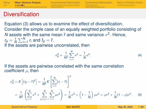
Diversification
Equation (3) allows us to examine the effect of diversification.Consider the simple case of an equally weighted portfolio consisting ofN assets with the same mean r and same variance σ2. Hence,rp = 1
N∑N
i=1 ri and rp = r .If the assets are pairwise uncorrelated, then
σ2p =
1N2
N∑i=1
σ2 =1Nσ2. (4)
If the assets are pairwise correlated with the same correlationcoefficient ρ, then
σ2p = E
[(rp − r)2
]=
1N2
E
N∑i=1
(ri − r)
2
=1
N2
N∑i=1
σ2 +N∑
j 6=i,j=1
N∑i=1
ρσ2
=1Nσ2 +
(1−
1N
)ρσ2 = ρσ2 +
1N
(1− ρ)σ2. (5)
QUANTITATIVE FINANCE SoF, SHUFE May 30, 2020 7 / 85
Setup Mean-Variance Analysis Unconstrained Optimization Constrained Optimization Back to Portfolio Choice
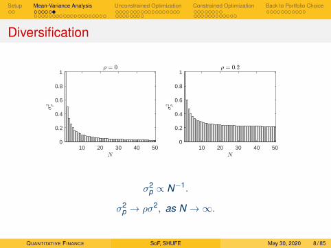
Diversification
10 20 30 40 500
0.2
0.4
0.6
0.8
1
10 20 30 40 500
0.2
0.4
0.6
0.8
1
σ2p ∝ N−1.
σ2p → ρσ2, as N →∞.
QUANTITATIVE FINANCE SoF, SHUFE May 30, 2020 8 / 85
Setup Mean-Variance Analysis Unconstrained Optimization Constrained Optimization Back to Portfolio Choice
The Markowitz Model
There are N assets with expected returns r1, r2, ..., rN , and covariancesσij = ρijσiσj , i , j = 1,2, ...,N.
A portfolio formed with the above assets is defined by the weightsw1,w2, ...,wN .
The quest is to find the minimum-variance portfolio for any (feasible)desired level of expected return.
QUANTITATIVE FINANCE SoF, SHUFE May 30, 2020 9 / 85
Setup Mean-Variance Analysis Unconstrained Optimization Constrained Optimization Back to Portfolio Choice
A Mathematical Formulation
Fix the expected return of a portfolio at rp. We need to find theminimum-variance portfolio that achieves rp.
minw1,w2,...,wN
12
N∑i=1
N∑j=1
wiσijwj , (6)
s.t .N∑
i=1
wi ri = rp,
N∑i=1
wi = 1.
The 1/2 is innocuous and just works to make the solution neater.
QUANTITATIVE FINANCE SoF, SHUFE May 30, 2020 10 / 85
Setup Mean-Variance Analysis Unconstrained Optimization Constrained Optimization Back to Portfolio Choice
Solution
The Markowitz Model provides the foundation for single-periodinvestment decisions by explicitly addressing the tradeoff betweenexpected return and variance of a portfolio.
We solve it using the Lagrangian method. We form the Lagrangian
L =12
N∑i=1
N∑j=1
wiσijwj − λ
(N∑
i=1
wi ri − rp
)− ζ
(N∑
i=1
wi − 1
), (7)
where λ and ζ are the Lagrangian Multipliers.
QUANTITATIVE FINANCE SoF, SHUFE May 30, 2020 11 / 85
Setup Mean-Variance Analysis Unconstrained Optimization Constrained Optimization Back to Portfolio Choice
Solution - continued
Differentiating the Lagrangian w.r.t. the weights and the multipliers, weget the following first order conditions (F.O.C.s).
N∑j=1
σijwj − λri − ζ = 0, for i = 1,2, ...,N, (8)
N∑i=1
wi ri = rp, (9)
N∑i=1
wi = 1. (10)
We use the fact σij = σji in (8). We have N + 2 linear equations forN + 2 unknowns. We can in principle solve the model with linearalgebra methods.
QUANTITATIVE FINANCE SoF, SHUFE May 30, 2020 12 / 85
Setup Mean-Variance Analysis Unconstrained Optimization Constrained Optimization Back to Portfolio Choice
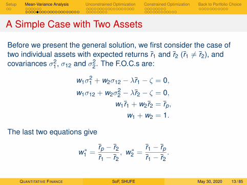
A Simple Case with Two Assets
Before we present the general solution, we first consider the case oftwo individual assets with expected returns r1 and r2 (r1 6= r2), andcovariances σ2
1, σ12 and σ22. The F.O.C.s are:
w1σ21 + w2σ12 − λr1 − ζ = 0,
w1σ12 + w2σ22 − λr2 − ζ = 0,
w1r1 + w2r2 = rp,
w1 + w2 = 1.
The last two equations give
w∗1 =rp − r2
r1 − r2, w∗2 =
r1 − rp
r1 − r2.
QUANTITATIVE FINANCE SoF, SHUFE May 30, 2020 13 / 85
Setup Mean-Variance Analysis Unconstrained Optimization Constrained Optimization Back to Portfolio Choice
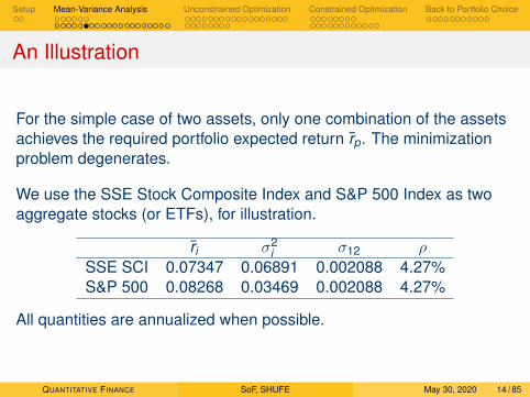
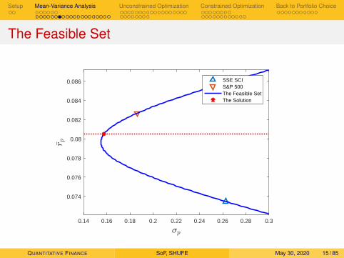
An Illustration
For the simple case of two assets, only one combination of the assetsachieves the required portfolio expected return rp. The minimizationproblem degenerates.
We use the SSE Stock Composite Index and S&P 500 Index as twoaggregate stocks (or ETFs), for illustration.
ri σ2i σ12 ρ
SSE SCI 0.07347 0.06891 0.002088 4.27%S&P 500 0.08268 0.03469 0.002088 4.27%
All quantities are annualized when possible.
QUANTITATIVE FINANCE SoF, SHUFE May 30, 2020 14 / 85
Setup Mean-Variance Analysis Unconstrained Optimization Constrained Optimization Back to Portfolio Choice
The Feasible Set
0.14 0.16 0.18 0.2 0.22 0.24 0.26 0.28 0.3
0.074
0.076
0.078
0.08
0.082
0.084
0.086 SSE SCIS&P 500The Feasible SetThe Solution
QUANTITATIVE FINANCE SoF, SHUFE May 30, 2020 15 / 85
Setup Mean-Variance Analysis Unconstrained Optimization Constrained Optimization Back to Portfolio Choice
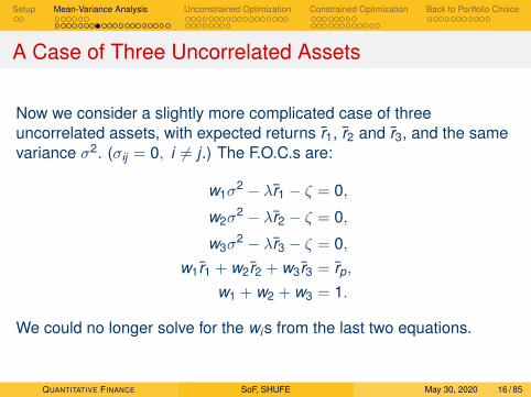
A Case of Three Uncorrelated Assets
Now we consider a slightly more complicated case of threeuncorrelated assets, with expected returns r1, r2 and r3, and the samevariance σ2. (σij = 0, i 6= j .) The F.O.C.s are:
w1σ2 − λr1 − ζ = 0,
w2σ2 − λr2 − ζ = 0,
w3σ2 − λr3 − ζ = 0,
w1r1 + w2r2 + w3r3 = rp,
w1 + w2 + w3 = 1.
We could no longer solve for the wis from the last two equations.
QUANTITATIVE FINANCE SoF, SHUFE May 30, 2020 16 / 85
Setup Mean-Variance Analysis Unconstrained Optimization Constrained Optimization Back to Portfolio Choice
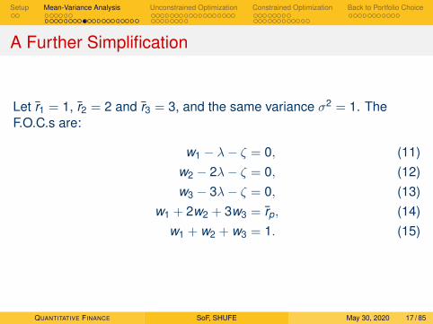
A Further Simplification
Let r1 = 1, r2 = 2 and r3 = 3, and the same variance σ2 = 1. TheF.O.C.s are:
w1 − λ− ζ = 0, (11)w2 − 2λ− ζ = 0, (12)w3 − 3λ− ζ = 0, (13)
w1 + 2w2 + 3w3 = rp, (14)w1 + w2 + w3 = 1. (15)
QUANTITATIVE FINANCE SoF, SHUFE May 30, 2020 17 / 85
Setup Mean-Variance Analysis Unconstrained Optimization Constrained Optimization Back to Portfolio Choice
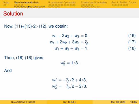
Solution
Now, (11)+(13)-2×(12), we obtain:
w1 − 2w2 + w3 = 0, (16)w1 + 2w2 + 3w3 = rp, (17)
w1 + w2 + w3 = 1. (18)
Then, (18)-(16) givesw∗2 = 1/3.
And
w∗1 = −rp/2 + 4/3,w∗3 = rp/2− 2/3.
QUANTITATIVE FINANCE SoF, SHUFE May 30, 2020 18 / 85
Setup Mean-Variance Analysis Unconstrained Optimization Constrained Optimization Back to Portfolio Choice
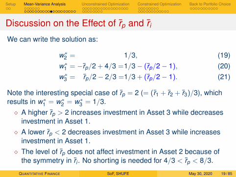
Discussion on the Effect of rp and ri
We can write the solution as:
w∗2 = 1/3, (19)w∗1 = −rp/2 + 4/3 =1/3− (rp/2− 1), (20)w∗3 = rp/2− 2/3 =1/3 + (rp/2− 1). (21)
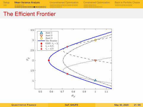
Note the interesting special case of rp = 2 (= (r1 + r2 + r3)/3), whichresults in w∗1 = w∗2 = w∗3 = 1/3.� A higher rp > 2 increases investment in Asset 3 while decreases
investment in Asset 1.� A lower rp < 2 decreases investment in Asset 3 while increases
investment in Asset 1.� The level of rp does not affect investment in Asset 2 because of
the symmetry in ri . No shorting is needed for 4/3 < rp < 8/3.
QUANTITATIVE FINANCE SoF, SHUFE May 30, 2020 19 / 85
Setup Mean-Variance Analysis Unconstrained Optimization Constrained Optimization Back to Portfolio Choice
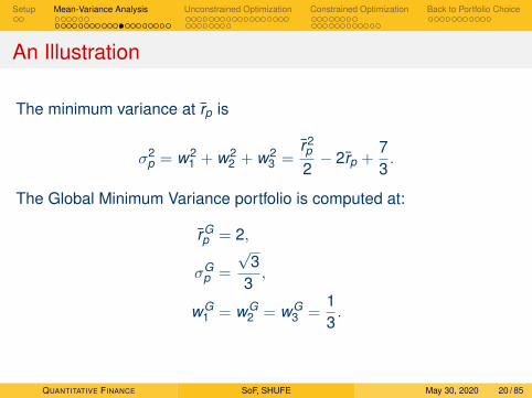
An Illustration
The minimum variance at rp is
σ2p = w2
1 + w22 + w2
3 =r2p
2− 2rp +
73.
The Global Minimum Variance portfolio is computed at:
rGp = 2,
σGp =
√3
3,
wG1 = wG
2 = wG3 =
13.
QUANTITATIVE FINANCE SoF, SHUFE May 30, 2020 20 / 85
Setup Mean-Variance Analysis Unconstrained Optimization Constrained Optimization Back to Portfolio Choice
The Efficient Frontier
0.5 0.6 0.7 0.8 0.9 1 1.1
1
1.5
2
2.5
3
3.5
QUANTITATIVE FINANCE SoF, SHUFE May 30, 2020 21 / 85
Setup Mean-Variance Analysis Unconstrained Optimization Constrained Optimization Back to Portfolio Choice
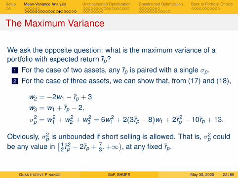
The Maximum Variance
We ask the opposite question: what is the maximum variance of aportfolio with expected return rp?
1 For the case of two assets, any rp is paired with a single σp.2 For the case of three assets, we can show that, from (17) and (18),
w2 = −2w1 − rp + 3w3 = w1 + rp − 2,
σ2p = w2
1 + w22 + w2
3 = 6w21 + 2(3rp − 8)w1 + 2r2
p − 10rp + 13.
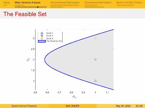
Obviously, σ2p is unbounded if short selling is allowed. That is, σ2
p couldbe any value in
[12 r2
p − 2rp + 73 ,+∞
), at any fixed rp.
QUANTITATIVE FINANCE SoF, SHUFE May 30, 2020 22 / 85
Setup Mean-Variance Analysis Unconstrained Optimization Constrained Optimization Back to Portfolio Choice
The Feasible Set
QUANTITATIVE FINANCE SoF, SHUFE May 30, 2020 23 / 85
Setup Mean-Variance Analysis Unconstrained Optimization Constrained Optimization Back to Portfolio Choice
No Short Selling Constraint
minw1,w2,...,wN
12
N∑i=1
N∑j=1
wiσijwj , (22)
s.t .N∑
i=1
wi ri = rp,
N∑i=1
wi = 1,
wi ≥ 0, for i = 1, 2, ...,N.
This is a Quadratic Program with a quadratic objective function andlinear equality and inequality constraints.We can solve it numerically, e.g., using Excel solver for a relativelysmall number of assets and other professional programs for hundredsor thousands of assets.
QUANTITATIVE FINANCE SoF, SHUFE May 30, 2020 24 / 85
Setup Mean-Variance Analysis Unconstrained Optimization Constrained Optimization Back to Portfolio Choice
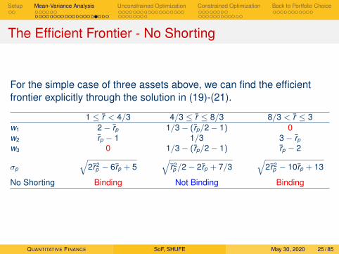
The Efficient Frontier - No Shorting
For the simple case of three assets above, we can find the efficientfrontier explicitly through the solution in (19)-(21).
1 ≤ r < 4/3 4/3 ≤ r ≤ 8/3 8/3 < r ≤ 3w1 2− rp 1/3− (rp/2− 1) 0w2 rp − 1 1/3 3− rp
w3 0 1/3− (rp/2− 1) rp − 2
σp
√2r 2
p − 6rp + 5√
r 2p /2− 2rp + 7/3
√2r 2
p − 10rp + 13
No Shorting Binding Not Binding Binding
QUANTITATIVE FINANCE SoF, SHUFE May 30, 2020 25 / 85
Setup Mean-Variance Analysis Unconstrained Optimization Constrained Optimization Back to Portfolio Choice
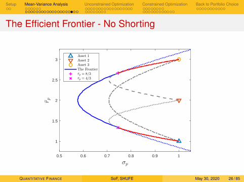
The Efficient Frontier - No Shorting
0.5 0.6 0.7 0.8 0.9 1
1
1.5
2
2.5
3
QUANTITATIVE FINANCE SoF, SHUFE May 30, 2020 26 / 85
Setup Mean-Variance Analysis Unconstrained Optimization Constrained Optimization Back to Portfolio Choice
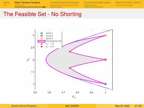
The Feasible Set - No Shorting
QUANTITATIVE FINANCE SoF, SHUFE May 30, 2020 27 / 85
Setup Mean-Variance Analysis Unconstrained Optimization Constrained Optimization Back to Portfolio Choice
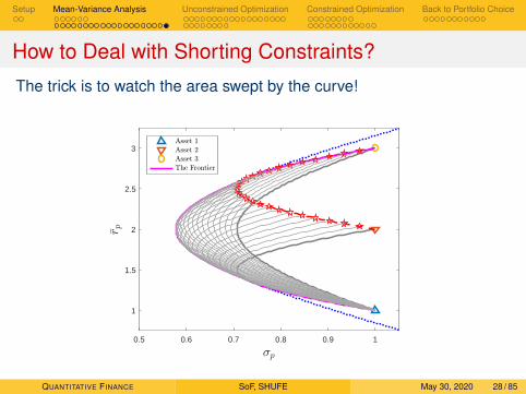
How to Deal with Shorting Constraints?
The trick is to watch the area swept by the curve!
0.5 0.6 0.7 0.8 0.9 1
1
1.5
2
2.5
3
QUANTITATIVE FINANCE SoF, SHUFE May 30, 2020 28 / 85
Setup Mean-Variance Analysis Unconstrained Optimization Constrained Optimization Back to Portfolio Choice
Unconstrained Optimization
A general mathematical formulation of multivariate unconstrainedoptimization is as follows.
minx∈Rn
f (x), (23)
where f (x) is the objective function.
Here, we assume all functions are well-behaved1, that is, sufficientlysmooth, e.g., twice-continuously differentiable.
Maximization problems can be transformed into equivalentminimizations by simply putting a negative sign before f (x).
maxx∈Rn
f (x) ⇔ minx∈Rn
−f (x). (24)
1Or the functions can be well approximated by well-behaved ones.QUANTITATIVE FINANCE SoF, SHUFE May 30, 2020 29 / 85
Setup Mean-Variance Analysis Unconstrained Optimization Constrained Optimization Back to Portfolio Choice
Univariate Minimization
A univariate unconstrained optimization problem considers anobjective function in one dimension.
minx∈R
f (x) (25)
Importance of univariate optimization:1 Many real problems corresponds to finding the optimum of
univariate functions (e.g., optimal hedge ratios of derivatives).2 Multivariable optimization methods in commercial use today
mostly contain a line search step.3 Fundamental ideas are best illustrated with univariate cases, and
they usually carry over to multivariate optimization.
QUANTITATIVE FINANCE SoF, SHUFE May 30, 2020 30 / 85
Setup Mean-Variance Analysis Unconstrained Optimization Constrained Optimization Back to Portfolio Choice
Solution
Definition of a solution x∗:(i) Global Minimum: There exists a point x∗ s.t. f (x∗) ≤ f (x), ∀x ∈ R.(ii) Strong Local minimum: There exists a point x∗ s.t. f (x∗) < f (x),∀x ∈ U(x∗), where U(x∗) is a neighbourhood of x∗.
(iii) Weak Local Minima: There exists a neighbourhood U(x∗) of x∗
s.t. f (x∗) ≤ f (x), ∀x ∈ U(x∗).
Clearly, (i) ; (ii), (ii) ; (i), (ii)⇒ (iii), (iii) ; (ii), (i)⇒ (iii), and(iii) ; (i).
QUANTITATIVE FINANCE SoF, SHUFE May 30, 2020 31 / 85
Setup Mean-Variance Analysis Unconstrained Optimization Constrained Optimization Back to Portfolio Choice
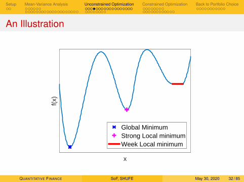
An Illustration
x
f(x)
Global MinimumStrong Local minimumWeek Local minimum
QUANTITATIVE FINANCE SoF, SHUFE May 30, 2020 32 / 85
Setup Mean-Variance Analysis Unconstrained Optimization Constrained Optimization Back to Portfolio Choice
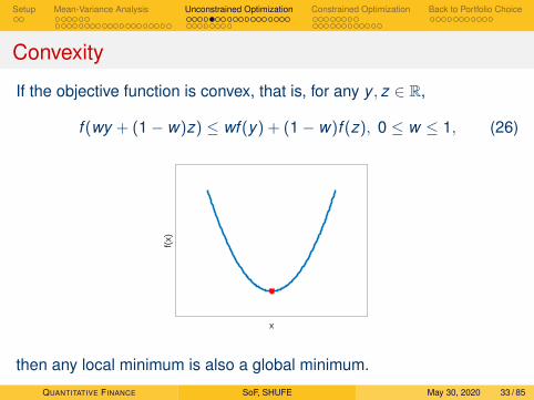
Convexity
If the objective function is convex, that is, for any y , z ∈ R,
f (wy + (1− w)z) ≤ wf (y) + (1− w)f (z), 0 ≤ w ≤ 1, (26)
x
f(x)
then any local minimum is also a global minimum.
QUANTITATIVE FINANCE SoF, SHUFE May 30, 2020 33 / 85
Setup Mean-Variance Analysis Unconstrained Optimization Constrained Optimization Back to Portfolio Choice
Discussion on Convexity
Convexity is a general concept used in optimization theory. Itdescribes the property of having an optimum for a function.
Convexity combines both stationarity (stable points) and curvature intoa single concept.
However, it is inconvenient to use for a specific function. For thewell-behaved functions considered here, first derivatives give us ameasure of the rate of change of the function. Second derivatives giveus a measure of curvature of the function or the rate of change of thefirst derivatives.
QUANTITATIVE FINANCE SoF, SHUFE May 30, 2020 34 / 85
Setup Mean-Variance Analysis Unconstrained Optimization Constrained Optimization Back to Portfolio Choice
Discussion on Convexity
x
f(x)
df(x)/dx>0
df(x)/dx<0
df(x)/dx=0,
d2f(x)/dx2>0
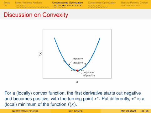
For a (locally) convex function, the first derivative starts out negativeand becomes positive, with the turning point x∗. Put differently, x∗ is a(local) minimum of the function f (x).
QUANTITATIVE FINANCE SoF, SHUFE May 30, 2020 35 / 85
Setup Mean-Variance Analysis Unconstrained Optimization Constrained Optimization Back to Portfolio Choice
Necessary and Sufficient Conditions for an Optimum
For a well-behaved twice continuously differentiable function f (x), thepoint x∗ is an optimum iff:
df (x)
dx
∣∣∣∣x∗
= 0 (stationarity),
and
d2f (x)
dx2
∣∣∣∣x∗> 0 (minimum),
or
d2f (x)
dx2
∣∣∣∣x∗< 0 (maximum).
QUANTITATIVE FINANCE SoF, SHUFE May 30, 2020 36 / 85
Setup Mean-Variance Analysis Unconstrained Optimization Constrained Optimization Back to Portfolio Choice
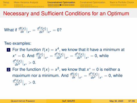
Necessary and Sufficient Conditions for an Optimum
What if df (x)dx
∣∣x∗ = d2f (x)
dx2
∣∣x∗ = 0?
Two examples:1 For the function f (x) = x4, we know that it have a minimum at
x∗ = 0. And df (x)dx
∣∣x∗ = d2f (x)
dx2
∣∣x∗ = d3f (x)
dx3
∣∣x∗ = 0, while
d4f (x)dx4
∣∣x∗ > 0.
2 For the function f (x) = x3, we know that x∗ = 0 is neither amaximum nor a minimum. And df (x)
dx
∣∣x∗ = d2f (x)
dx2
∣∣x∗ = 0, while
d3f (x)dx3
∣∣x∗ > 0.
QUANTITATIVE FINANCE SoF, SHUFE May 30, 2020 37 / 85
Setup Mean-Variance Analysis Unconstrained Optimization Constrained Optimization Back to Portfolio Choice
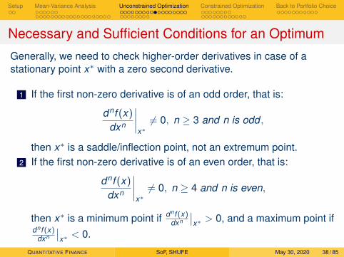
Necessary and Sufficient Conditions for an Optimum
Generally, we need to check higher-order derivatives in case of astationary point x∗ with a zero second derivative.
1 If the first non-zero derivative is of an odd order, that is:
dnf (x)
dxn
∣∣∣∣x∗6= 0, n ≥ 3 and n is odd ,
then x∗ is a saddle/inflection point, not an extremum point.2 If the first non-zero derivative is of an even order, that is:
dnf (x)
dxn
∣∣∣∣x∗6= 0, n ≥ 4 and n is even,
then x∗ is a minimum point if dnf (x)dxn
∣∣x∗ > 0, and a maximum point if
dnf (x)dxn
∣∣x∗ < 0.
QUANTITATIVE FINANCE SoF, SHUFE May 30, 2020 38 / 85
Setup Mean-Variance Analysis Unconstrained Optimization Constrained Optimization Back to Portfolio Choice
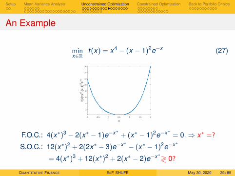
An Example
minx∈R
f (x) = x4 − (x − 1)2e−x (27)
-1 -0.5 0 0.5 1 1.5 2
x
2
4
6
8
10
12
14
16
f(x)
=x4
-(x-
1)2e-x
F.O.C.: 4(x∗)3 − 2(x∗ − 1)e−x∗ + (x∗ − 1)2e−x∗ = 0.⇒ x∗ =?
S.O.C.: 12(x∗)2 + 2(2x∗ − 3)e−x∗ − (x∗ − 1)2e−x∗
= 4(x∗)3 + 12(x∗)2 + 2(x∗ − 2)e−x∗≷ 0?
QUANTITATIVE FINANCE SoF, SHUFE May 30, 2020 39 / 85
Setup Mean-Variance Analysis Unconstrained Optimization Constrained Optimization Back to Portfolio Choice
Discussions
Three observations:1 The F.O.C. may be a nonlinear equation which is often as difficult
to solve as the original optimization problem.2 The sign of higher-order derivatives may be difficult to determine.3 In practical problems, the objective functions and the derivatives
may only be computed numerically.In sum, unconstrained univariate optimization problems may not be asstraightforward as you thought.
QUANTITATIVE FINANCE SoF, SHUFE May 30, 2020 40 / 85
Setup Mean-Variance Analysis Unconstrained Optimization Constrained Optimization Back to Portfolio Choice
Multivariate Optimization
Now we extend to unconstrained minimization of a function in ndimensions.
minx∈Rn
f (x), (28)
where f (x) is the twice-continuously differentiable objective function.
We can likewise define global, weak local, and strong local minima, aswell as convexity, in n dimensions.
QUANTITATIVE FINANCE SoF, SHUFE May 30, 2020 41 / 85
Setup Mean-Variance Analysis Unconstrained Optimization Constrained Optimization Back to Portfolio Choice
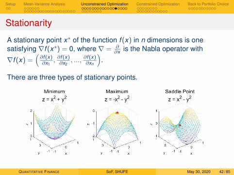
Stationarity
A stationary point x∗ of the function f (x) in n dimensions is onesatisfying ∇f (x∗) = 0, where ∇ = ∂
∂x is the Nabla operator with
∇f (x) =(∂f (x)∂x1
, ∂f (x)∂x2
, ..., ∂f (x)∂xn
).
There are three types of stationary points.
QUANTITATIVE FINANCE SoF, SHUFE May 30, 2020 42 / 85
Setup Mean-Variance Analysis Unconstrained Optimization Constrained Optimization Back to Portfolio Choice
Necessary Conditions for an Optimum
The conditions are simply multivariate extensions of univariate ones.
Necessary conditions for a weak local minimum
C1. ∇f (x∗) = 0 (stationarity).C2. ∇2f (x∗) is positive semi-definite. That is, v>∇2f (x∗)v ≥ 0, for alln × 1 vector v 6= 0.
Here, ∇2f (x) =
∂2f (x)
∂x21
∂2f (x)∂x1∂x2
· · · ∂2f (x)∂x1∂xn
∂2f (x)∂x2∂x1
∂2f (x)
∂x22· · · ∂2f (x)
∂x2∂xn
· · · · · · · · · · · ·∂2f (x)∂xn∂x1
∂2f (x)∂xn∂x2
· · · ∂2f (x)
∂x2n
.It is called the Hessian Matrix after German mathematician LudwigOtto Hesse. It describes the local curvature of f (x).
QUANTITATIVE FINANCE SoF, SHUFE May 30, 2020 43 / 85
Setup Mean-Variance Analysis Unconstrained Optimization Constrained Optimization Back to Portfolio Choice
Sufficient Conditions for an Optimum
The conditions are again simply multivariate extensions of univariateones.
Sufficient conditions for a strong local minimum
C1. ∇f (x∗) = 0 (stationarity).C2. ∇2f (x∗) is positive definite. That is, v>∇2f (x∗)v > 0, for all n × 1vector v 6= 0.
QUANTITATIVE FINANCE SoF, SHUFE May 30, 2020 44 / 85
Setup Mean-Variance Analysis Unconstrained Optimization Constrained Optimization Back to Portfolio Choice
The Recipe
1 Correctly formulate the optimization problem.2 Find a point x∗ that could potentially be a solution (satisfying the
necessary conditions).3 Verify this point x∗ is certainly a solution (satisfying the sufficient
conditions).
QUANTITATIVE FINANCE SoF, SHUFE May 30, 2020 45 / 85
Setup Mean-Variance Analysis Unconstrained Optimization Constrained Optimization Back to Portfolio Choice
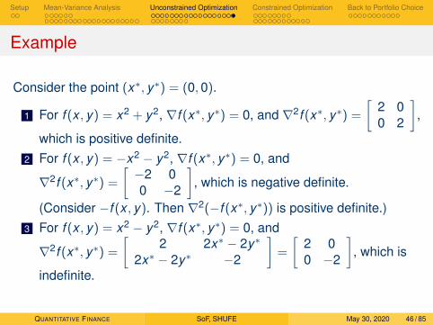
Example
Consider the point (x∗, y∗) = (0,0).
1 For f (x , y) = x2 + y2, ∇f (x∗, y∗) = 0, and ∇2f (x∗, y∗) =
[2 00 2
],
which is positive definite.2 For f (x , y) = −x2 − y2, ∇f (x∗, y∗) = 0, and
∇2f (x∗, y∗) =
[−2 00 −2
], which is negative definite.
(Consider −f (x , y). Then ∇2(−f (x∗, y∗)) is positive definite.)3 For f (x , y) = x2 − y2, ∇f (x∗, y∗) = 0, and
∇2f (x∗, y∗) =
[2 2x∗ − 2y∗
2x∗ − 2y∗ −2
]=
[2 00 −2
], which is
indefinite.
QUANTITATIVE FINANCE SoF, SHUFE May 30, 2020 46 / 85
Setup Mean-Variance Analysis Unconstrained Optimization Constrained Optimization Back to Portfolio Choice
A Different Perspective
Before we turn to constrained optimization, we provide another intuitivediscussion of the methods we covered for unconstrained optimization.Again, it would help us understand the unconstrained approach, andmore importantly, it can be easily extended to the constrained situation.
We would understand what the second order conditions for optimalityare and also why they are. We will use an algebraic approach,exploiting the matrix of second derivatives called the Hessian matrix.Then we will see later that the conditions for the constrained case canbe easily stated in terms of a bordered Hessian matrix2.
2Many applied mathematics students use it for a long time without knowing itsrelevance.
QUANTITATIVE FINANCE SoF, SHUFE May 30, 2020 47 / 85
Setup Mean-Variance Analysis Unconstrained Optimization Constrained Optimization Back to Portfolio Choice
The Univariate Case
The 2nd order approximation to f (x) near x is
f (x) = f (x) + fx (x)(x − x) +12
fxx (x)(x − x)2. (29)
Hence,
df = fx (x)dx +12
fxx (x)(dx)2, (30)
where df = f (x)− f (x) and dx = x − x .
QUANTITATIVE FINANCE SoF, SHUFE May 30, 2020 48 / 85
Setup Mean-Variance Analysis Unconstrained Optimization Constrained Optimization Back to Portfolio Choice
The Univariate Case
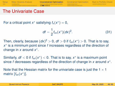
For a critical point x∗ satisfying fx (x∗) = 0,
df =12
fxx (x∗)(dx)2. (31)
Then, clearly, because (dx)2 > 0, df > 0 if fxx (x∗) > 0. That is to say,x∗ is a minimum point since f increases regardless of the direction ofchange in x around x∗.
Similarly, df < 0 if fxx (x∗) < 0. That is to say, x∗ is a maximum pointsince f decreases regardless of the direction of change in x around x∗.
Note that the Hessian matrix for the univariate case is just the 1× 1matrix [fxx (x∗)].
QUANTITATIVE FINANCE SoF, SHUFE May 30, 2020 49 / 85
Setup Mean-Variance Analysis Unconstrained Optimization Constrained Optimization Back to Portfolio Choice
The Two-Variable Case
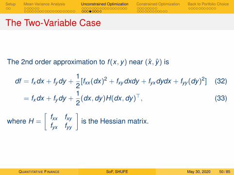
The 2nd order approximation to f (x , y) near (x , y) is
df = fxdx + fydy +12
[fxx (dx)2 + fxydxdy + fyxdydx + fyy (dy)2] (32)
= fxdx + fydy +12
(dx ,dy)H(dx ,dy)>, (33)
where H =
[fxx fxyfyx fyy
]is the Hessian matrix.
QUANTITATIVE FINANCE SoF, SHUFE May 30, 2020 50 / 85
Setup Mean-Variance Analysis Unconstrained Optimization Constrained Optimization Back to Portfolio Choice
The Two-Variable Case
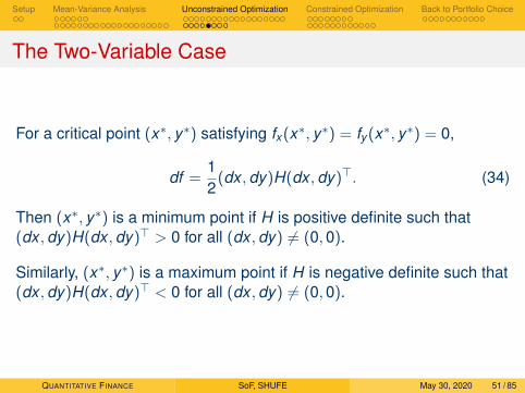
For a critical point (x∗, y∗) satisfying fx (x∗, y∗) = fy (x∗, y∗) = 0,
df =12
(dx ,dy)H(dx ,dy)>. (34)
Then (x∗, y∗) is a minimum point if H is positive definite such that(dx ,dy)H(dx ,dy)> > 0 for all (dx ,dy) 6= (0,0).
Similarly, (x∗, y∗) is a maximum point if H is negative definite such that(dx ,dy)H(dx ,dy)> < 0 for all (dx ,dy) 6= (0,0).
QUANTITATIVE FINANCE SoF, SHUFE May 30, 2020 51 / 85
Setup Mean-Variance Analysis Unconstrained Optimization Constrained Optimization Back to Portfolio Choice
Exercise 2Do the analysis for the three-variable case.
QUANTITATIVE FINANCE SoF, SHUFE May 30, 2020 52 / 85

Setup Mean-Variance Analysis Unconstrained Optimization Constrained Optimization Back to Portfolio Choice
Exercise 2Do the analysis for the three-variable case.
The 2nd order approximation to f (x , y , z) near (x , y , z) is
df = fxdx + fydy + fzdz +12
(dx ,dy ,dz)H(dx ,dy ,dz)>, (35)
where H =
fxx fxy fxzfyx fyy fyzfzx fzy fzz
is the Hessian matrix.
For a critical point (x∗, y∗, z∗) satisfying fx = fy = fz = 0,
df =12
(dx ,dy ,dz)H(dx ,dy ,dz)>. (36)
Hence (x∗, y∗, z∗) is a minimum point if H is positive definite, and amaximum point if H is negative definite.
QUANTITATIVE FINANCE SoF, SHUFE May 30, 2020 53 / 85
Setup Mean-Variance Analysis Unconstrained Optimization Constrained Optimization Back to Portfolio Choice
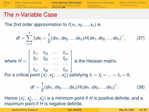
The n-Variable Case
The 2nd order approximation to f (x1, x2, ..., xn) is
df =n∑
i=1
fidxi +12
(dx1,dx2, ...,dxn)H(dx1,dx2, ...,dxn)>, (37)
where H =
f11 f12 · · · f1nf21 f22 · · · f2n· · · · · · · · · · · ·fn1 fn2 · · · fnn
is the Hessian matrix.
For a critical point (x∗1 , x∗2 , ..., x
∗n ) satisfying f1 = f2 = ... = fn = 0,
df =12
(dx1,dx2, ...,dxn)H(dx1,dx2, ...,dxn)>. (38)
Hence (x∗1 , x∗2 , ..., x
∗n ) is a minimum point if H is positive definite, and a
maximum point if H is negative definite.QUANTITATIVE FINANCE SoF, SHUFE May 30, 2020 54 / 85
Setup Mean-Variance Analysis Unconstrained Optimization Constrained Optimization Back to Portfolio Choice
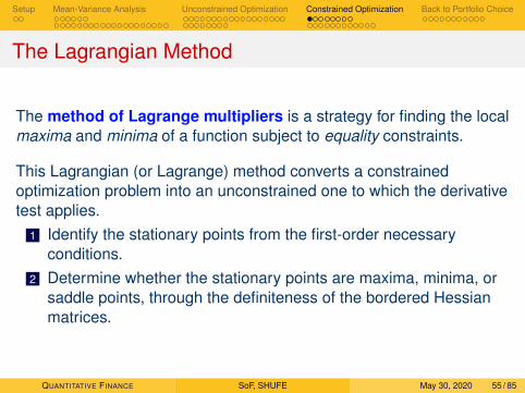
The Lagrangian Method
The method of Lagrange multipliers is a strategy for finding the localmaxima and minima of a function subject to equality constraints.
This Lagrangian (or Lagrange) method converts a constrainedoptimization problem into an unconstrained one to which the derivativetest applies.
1 Identify the stationary points from the first-order necessaryconditions.
2 Determine whether the stationary points are maxima, minima, orsaddle points, through the definiteness of the bordered Hessianmatrices.
QUANTITATIVE FINANCE SoF, SHUFE May 30, 2020 55 / 85
Setup Mean-Variance Analysis Unconstrained Optimization Constrained Optimization Back to Portfolio Choice
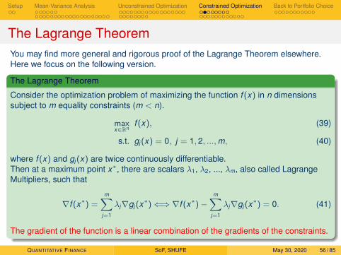
The Lagrange TheoremYou may find more general and rigorous proof of the Lagrange Theorem elsewhere.Here we focus on the following version.
The Lagrange Theorem
Consider the optimization problem of maximizing the function f (x) in n dimensionssubject to m equality constraints (m < n).
maxx∈Rn
f (x), (39)
s.t. gj (x) = 0, j = 1, 2, ...,m, (40)
where f (x) and gj (x) are twice continuously differentiable.Then at a maximum point x∗, there are scalars λ1, λ2, ..., λm, also called LagrangeMultipliers, such that
∇f (x∗) =m∑
j=1
λj∇gj (x∗)⇐⇒ ∇f (x∗)−m∑
j=1
λj∇gj (x∗) = 0. (41)
The gradient of the function is a linear combination of the gradients of the constraints.
QUANTITATIVE FINANCE SoF, SHUFE May 30, 2020 56 / 85
Setup Mean-Variance Analysis Unconstrained Optimization Constrained Optimization Back to Portfolio Choice
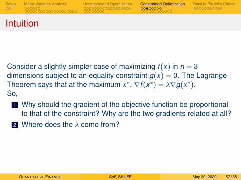
Intuition
Consider a slightly simpler case of maximizing f (x) in n = 3dimensions subject to an equality constraint g(x) = 0. The LagrangeTheorem says that at the maximum x∗, ∇f (x∗) = λ∇g(x∗).So,
1 Why should the gradient of the objective function be proportionalto that of the constraint? Why are the two gradients related at all?
2 Where does the λ come from?
QUANTITATIVE FINANCE SoF, SHUFE May 30, 2020 57 / 85
Setup Mean-Variance Analysis Unconstrained Optimization Constrained Optimization Back to Portfolio Choice
Intuition: For the Case of a Single Constraint
1 The set of points satisfying g(x) = 0 is a surface in 3 dimensions,or a (maybe oddly shaped) balloon.
2 The set of points satisfying f (x) = k is another surface in 3dimensions, or another (maybe oddly shaped) balloon.
3 Take k to be a very large number, larger than the maximum of f (x)under the constraint. Then the Balloon g(x) = 0 lies inside theballoon f (x) = k .
QUANTITATIVE FINANCE SoF, SHUFE May 30, 2020 58 / 85
Setup Mean-Variance Analysis Unconstrained Optimization Constrained Optimization Back to Portfolio Choice
Intuition: For the Case of a Single Constraint
4 Now gradually shrink k , by leaking the air in the outer balloon. Atsome point, the outer balloon will touch the inner one at themaximum under constraint.
5 At the touching point of the maximum, the two balloons should betangent, hence their normal vectors, given by their gradients,should be both perpendicular to the same tangent plane thusparallel to each other.
6 Recall the Geometrical interpretation of a gradient: The directionof the gradient is the direction of fastest increase of the function ata certain point, and its magnitude is the rate of increase in thatdirection.
7 Hence, in contrast to the direction of increase, f (x) and g(x) neednot have the same rate of increase since the two balloons mayhave different shapes. The scaling constant λ results.
This explanation works for any n if you think of hyper-balloons.QUANTITATIVE FINANCE SoF, SHUFE May 30, 2020 59 / 85
Setup Mean-Variance Analysis Unconstrained Optimization Constrained Optimization Back to Portfolio Choice
A Pictorial Illustration
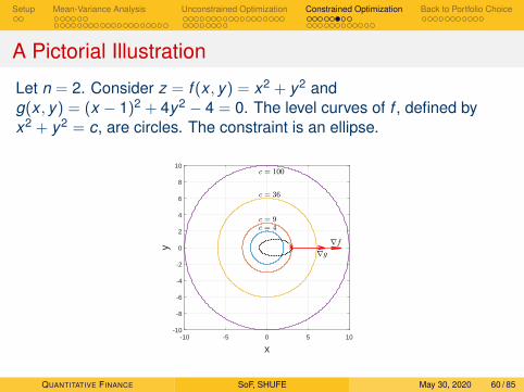
Let n = 2. Consider z = f (x , y) = x2 + y2 andg(x , y) = (x − 1)2 + 4y2 − 4 = 0. The level curves of f , defined byx2 + y2 = c, are circles. The constraint is an ellipse.
-10 -5 0 5 10
x
-10
-8
-6
-4
-2
0
2
4
6
8
10y
QUANTITATIVE FINANCE SoF, SHUFE May 30, 2020 60 / 85
Setup Mean-Variance Analysis Unconstrained Optimization Constrained Optimization Back to Portfolio Choice
Intuition: For the Case of Multiple Constraints
Once we understood the case with one constraint, extension tomultiple constraints are straightforward.
Consider the case of maximizing f (x) in n dimensions subject to mequality constraints gj(x) = 0.
1 The Lagrange Theorem says that at the maximum x∗,∇f (x∗) =
∑mj=1 λj∇gj(x∗).
2 This tells us that any direction of change that is perpendicular toall the gradients ∇gj must be perpendicular to the gradient ∇f aswell.
3 This in turn means that you cannot increase f without violating atleast one of the constraints.
QUANTITATIVE FINANCE SoF, SHUFE May 30, 2020 61 / 85
Setup Mean-Variance Analysis Unconstrained Optimization Constrained Optimization Back to Portfolio Choice
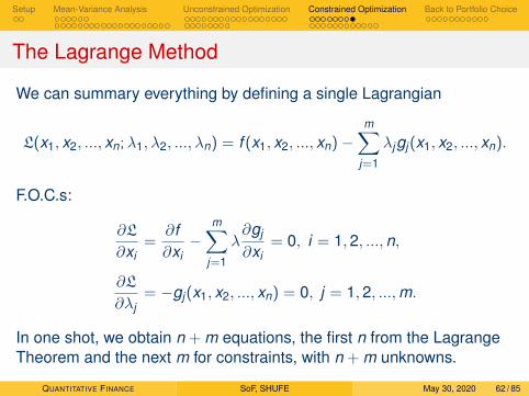
The Lagrange Method
We can summary everything by defining a single Lagrangian
L(x1, x2, ..., xn;λ1, λ2, ..., λn) = f (x1, x2, ..., xn)−m∑
j=1
λjgj(x1, x2, ..., xn).
F.O.C.s:
∂L
∂xi=
∂f∂xi−
m∑j=1
λ∂gj
∂xi= 0, i = 1,2, ...,n,
∂L
∂λj= −gj(x1, x2, ..., xn) = 0, j = 1,2, ...,m.
In one shot, we obtain n + m equations, the first n from the LagrangeTheorem and the next m for constraints, with n + m unknowns.
QUANTITATIVE FINANCE SoF, SHUFE May 30, 2020 62 / 85
Setup Mean-Variance Analysis Unconstrained Optimization Constrained Optimization Back to Portfolio Choice
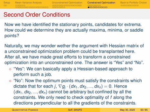
Second Order Conditions
Now we have identified the stationary points, candidates for extrema.How could we determine they are actually maxima, minima, or saddlepoints?
Naturally, we may wonder wether the argument with Hessian matrix ofa unconstrained optimization problem could be transplanted here.After all, we have made great efforts to transform a constrainedoptimization into an unconstrained one. The answer is “Yes” and “No”.� “Yes”: We can basically apply a Hessian-based approach to
perform such a job.� “No”: Now the optimum points must satisfy the constraints which
dictate that for each j , ∇gj · (dx1,dx2, ...,dxn) = 0. Hence(dx1,dx2, ...,dxn) cannot be arbitrary but confined by all theconstraints. We only need to check optimality of f along thedirections perpendicular to all the gradients of the constraints.
QUANTITATIVE FINANCE SoF, SHUFE May 30, 2020 63 / 85
Setup Mean-Variance Analysis Unconstrained Optimization Constrained Optimization Back to Portfolio Choice
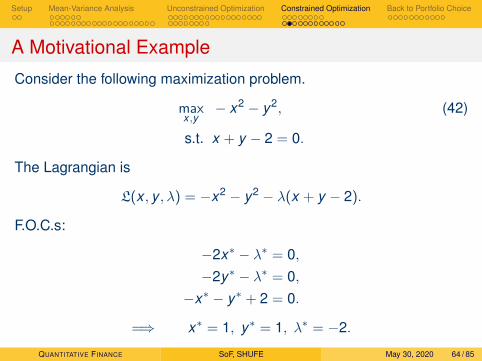
A Motivational Example
Consider the following maximization problem.
maxx ,y
− x2 − y2, (42)
s.t. x + y − 2 = 0.
The Lagrangian is
L(x , y , λ) = −x2 − y2 − λ(x + y − 2).
F.O.C.s:
−2x∗ − λ∗ = 0,−2y∗ − λ∗ = 0,
−x∗ − y∗ + 2 = 0.
=⇒ x∗ = 1, y∗ = 1, λ∗ = −2.
QUANTITATIVE FINANCE SoF, SHUFE May 30, 2020 64 / 85
Setup Mean-Variance Analysis Unconstrained Optimization Constrained Optimization Back to Portfolio Choice
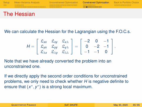
The Hessian
We can calculate the Hessian for the Lagrangian using the F.O.C.s.
H =
Lxx Lxy LxλLyx Lyy LyλLλx Lλy Lλλ
=
−2 0 −10 −2 −1−1 −1 0
.Note that we have already converted the problem into anunconstrained one.
If we directly apply the second order conditions for unconstrainedproblems, we only need to check whether H is negative definite toensure that (x∗, y∗) is a strong local maximum.
QUANTITATIVE FINANCE SoF, SHUFE May 30, 2020 65 / 85
Setup Mean-Variance Analysis Unconstrained Optimization Constrained Optimization Back to Portfolio Choice
The Hessian
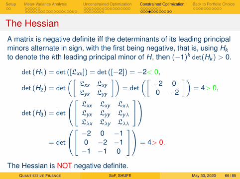
A matrix is negative definite iff the determinants of its leading principalminors alternate in sign, with the first being negative, that is, using Hkto denote the k th leading principal minor of H, then (−1)k det(Hk ) > 0.
det (H1) = det ([Lxx ]) = det ([−2]) = −2< 0,
det (H2) = det
([Lxx LxyLyx Lyy
])= det
([−2 00 −2
])= 4> 0,
det (H3) = det
Lxx Lxy LxλLyx Lyy LyλLλx Lλy Lλλ
= det
−2 0 −10 −2 −1−1 −1 0
= 4> 0.
The Hessian is NOT negative definite.QUANTITATIVE FINANCE SoF, SHUFE May 30, 2020 66 / 85
Setup Mean-Variance Analysis Unconstrained Optimization Constrained Optimization Back to Portfolio Choice
The Bordered Hessian
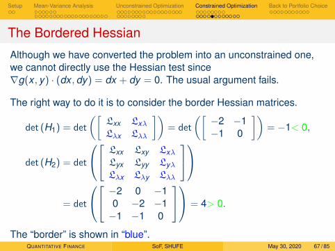
Although we have converted the problem into an unconstrained one,we cannot directly use the Hessian test since∇g(x , y) · (dx ,dy) = dx + dy = 0. The usual argument fails.
The right way to do it is to consider the border Hessian matrices.
det (H1) = det
([Lxx LxλLλx Lλλ
])= det
([−2 −1−1 0
])= −1< 0,
det (H2) = det
Lxx Lxy LxλLyx Lyy LyλLλx Lλy Lλλ
= det
−2 0 −10 −2 −1−1 −1 0
= 4> 0.
The “border” is shown in “blue”.QUANTITATIVE FINANCE SoF, SHUFE May 30, 2020 67 / 85
Setup Mean-Variance Analysis Unconstrained Optimization Constrained Optimization Back to Portfolio Choice
The Bordered Hessian - General Result
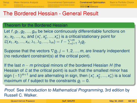
Theorem for the Bordered HessianLet f ,g1,g2, ...,gm be twice continuously differentiable functions onx1, x2, ..., xn, and (x∗1 , x
∗2 , ..., x
∗n ) is a critical/stationary point for
L(x1, x2, ..., xn;λ1, λ2, ..., λm) = f −∑m
j=1 λjgj .
Suppose that the vectors ∇gj , j = 1,2, ...,m, are linearly independent(no redundant constraint(s) at the critical point).
If the last n −m principal minors of the bordered Hessian H (theHessian of L at the critical point) is such that the smallest minor hassign (−1)m+1 and are alternating in sign, then (x∗1 , x
∗2 , ..., x
∗n ) is a local
maximum of f subject to the constraints gj = 0.
Proof. See Introduction to Mathematical Programming, 3rd edition byRussell C. Walker.
QUANTITATIVE FINANCE SoF, SHUFE May 30, 2020 68 / 85
Setup Mean-Variance Analysis Unconstrained Optimization Constrained Optimization Back to Portfolio Choice
The Bordered Hessian - General Result
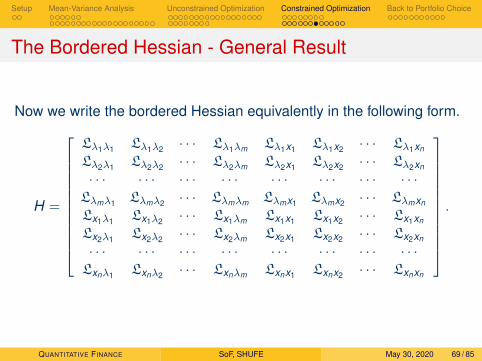
Now we write the bordered Hessian equivalently in the following form.
H =
Lλ1λ1 Lλ1λ2 · · · Lλ1λm Lλ1x1 Lλ1x2 · · · Lλ1xn
Lλ2λ1 Lλ2λ2 · · · Lλ2λm Lλ2x1 Lλ2x2 · · · Lλ2xn
· · · · · · · · · · · · · · · · · · · · · · · ·Lλmλ1 Lλmλ2 · · · Lλmλm Lλmx1 Lλmx2 · · · Lλmxn
Lx1λ1 Lx1λ2 · · · Lx1λm Lx1x1 Lx1x2 · · · Lx1xn
Lx2λ1 Lx2λ2 · · · Lx2λm Lx2x1 Lx2x2 · · · Lx2xn
· · · · · · · · · · · · · · · · · · · · · · · ·Lxnλ1 Lxnλ2 · · · Lxnλm Lxnx1 Lxnx2 · · · Lxnxn
.
QUANTITATIVE FINANCE SoF, SHUFE May 30, 2020 69 / 85
Setup Mean-Variance Analysis Unconstrained Optimization Constrained Optimization Back to Portfolio Choice
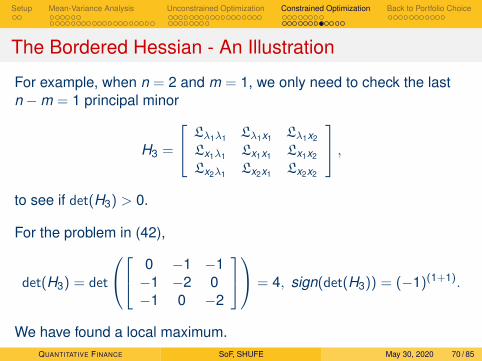
The Bordered Hessian - An Illustration
For example, when n = 2 and m = 1, we only need to check the lastn −m = 1 principal minor
H3 =
Lλ1λ1 Lλ1x1 Lλ1x2
Lx1λ1 Lx1x1 Lx1x2
Lx2λ1 Lx2x1 Lx2x2
,to see if det(H3) > 0.
For the problem in (42),
det(H3) = det
0 −1 −1−1 −2 0−1 0 −2
= 4, sign(det(H3)) = (−1)(1+1).
We have found a local maximum.QUANTITATIVE FINANCE SoF, SHUFE May 30, 2020 70 / 85
Setup Mean-Variance Analysis Unconstrained Optimization Constrained Optimization Back to Portfolio Choice
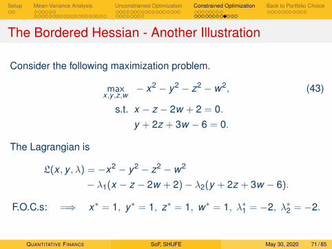
The Bordered Hessian - Another Illustration
Consider the following maximization problem.
maxx ,y ,z,w
− x2 − y2 − z2 − w2, (43)
s.t. x − z − 2w + 2 = 0.y + 2z + 3w − 6 = 0.
The Lagrangian is
L(x , y , λ) = −x2 − y2 − z2 − w2
− λ1(x − z − 2w + 2)− λ2(y + 2z + 3w − 6).
F.O.C.s: =⇒ x∗ = 1, y∗ = 1, z∗ = 1, w∗ = 1, λ∗1 = −2, λ∗2 = −2.
QUANTITATIVE FINANCE SoF, SHUFE May 30, 2020 71 / 85
Setup Mean-Variance Analysis Unconstrained Optimization Constrained Optimization Back to Portfolio Choice
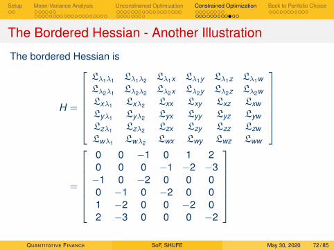
The Bordered Hessian - Another Illustration
The bordered Hessian is
H =
Lλ1λ1 Lλ1λ2 Lλ1x Lλ1y Lλ1z Lλ1wLλ2λ1 Lλ2λ2 Lλ2x Lλ2y Lλ2z Lλ2wLxλ1 Lxλ2 Lxx Lxy Lxz LxwLyλ1 Lyλ2 Lyx Lyy Lyz LywLzλ1 Lzλ2 Lzx Lzy Lzz LzwLwλ1 Lwλ2 Lwx Lwy Lwz Lww
=
0 0 −1 0 1 20 0 0 −1 −2 −3−1 0 −2 0 0 00 −1 0 −2 0 01 −2 0 0 −2 02 −3 0 0 0 −2
QUANTITATIVE FINANCE SoF, SHUFE May 30, 2020 72 / 85
Setup Mean-Variance Analysis Unconstrained Optimization Constrained Optimization Back to Portfolio Choice
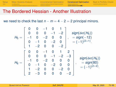
The Bordered Hessian - Another Illustration
we need to check the last n −m = 4− 2 = 2 principal minors.
H5 =
0 0 −1 0 10 0 0 −1 −2−1 0 −2 0 00 −1 0 −2 01 −2 0 0 −2
,sign(det(H5))= sign(−12)
= (−1)(2+1).
H6 =
0 0 −1 0 1 20 0 0 −1 −2 −3−1 0 −2 0 0 00 −1 0 −2 0 01 −2 0 0 −2 02 −3 0 0 0 −2
,sign(det(H6))
= sign(80)
= (−1)(2+2).
QUANTITATIVE FINANCE SoF, SHUFE May 30, 2020 73 / 85
Setup Mean-Variance Analysis Unconstrained Optimization Constrained Optimization Back to Portfolio Choice
A Final Word
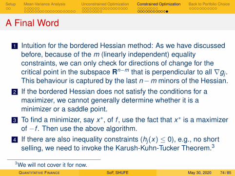
1 Intuition for the bordered Hessian method: As we have discussedbefore, because of the m (linearly independent) equalityconstraints, we can only check for directions of change for thecritical point in the subspace Rn−m that is perpendicular to all ∇gj .This behaviour is captured by the last n−m minors of the Hessian.
2 If the bordered Hessian does not satisfy the conditions for amaximizer, we cannot generally determine whether it is aminimizer or a saddle point.
3 To find a minimizer, say x∗, of f , use the fact that x∗ is a maximizerof −f . Then use the above algorithm.
4 If there are also inequality constraints (hj(x) ≤ 0), e.g., no shortselling, we need to invoke the Karush-Kuhn-Tucker Theorem.3
3We will not cover it for now.QUANTITATIVE FINANCE SoF, SHUFE May 30, 2020 74 / 85
Setup Mean-Variance Analysis Unconstrained Optimization Constrained Optimization Back to Portfolio Choice
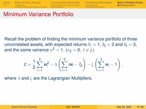
Minimum Variance Portfolio
Recall the problem of finding the minimum variance portfolio of threeuncorrelated assets, with expected returns r1 = 1, r2 = 2 and r3 = 3,and the same variance σ2 = 1. (σij = 0, i 6= j .)
L =12
3∑i=1
w2i − λ
(3∑
i=1
iwi − rp
)− ζ
(3∑
i=1
wi − 1
),
where λ and ζ are the Lagrangian Multipliers.
QUANTITATIVE FINANCE SoF, SHUFE May 30, 2020 75 / 85
Setup Mean-Variance Analysis Unconstrained Optimization Constrained Optimization Back to Portfolio Choice
Minimum Variance Portfolio
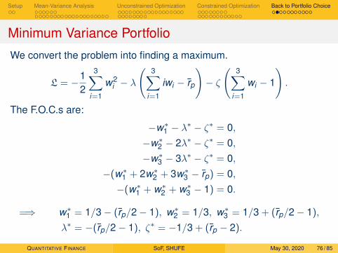
We convert the problem into finding a maximum.
L = −12
3∑i=1
w2i − λ
(3∑
i=1
iwi − rp
)− ζ
(3∑
i=1
wi − 1
).
The F.O.C.s are:
−w∗1 − λ∗ − ζ∗ = 0,−w∗2 − 2λ∗ − ζ∗ = 0,−w∗3 − 3λ∗ − ζ∗ = 0,
−(w∗1 + 2w∗2 + 3w∗3 − rp) = 0,−(w∗1 + w∗2 + w∗3 − 1) = 0.
=⇒ w∗1 = 1/3− (rp/2− 1), w∗2 = 1/3, w∗3 = 1/3 + (rp/2− 1),
λ∗ = −(rp/2− 1), ζ∗ = −1/3 + (rp − 2).
QUANTITATIVE FINANCE SoF, SHUFE May 30, 2020 76 / 85
Setup Mean-Variance Analysis Unconstrained Optimization Constrained Optimization Back to Portfolio Choice
Minimum Variance Portfolio
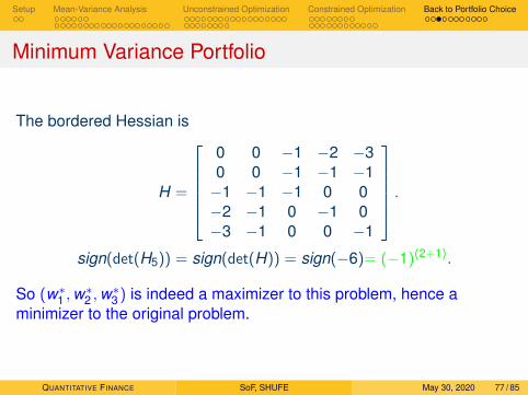
The bordered Hessian is
H =
0 0 −1 −2 −30 0 −1 −1 −1−1 −1 −1 0 0−2 −1 0 −1 0−3 −1 0 0 −1
.sign(det(H5)) = sign(det(H)) = sign(−6)= (−1)(2+1).
So (w∗1 ,w∗2 ,w
∗3 ) is indeed a maximizer to this problem, hence a
minimizer to the original problem.
QUANTITATIVE FINANCE SoF, SHUFE May 30, 2020 77 / 85
Setup Mean-Variance Analysis Unconstrained Optimization Constrained Optimization Back to Portfolio Choice
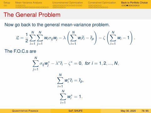
The General Problem
Now go back to the general mean-variance problem.
L =12
N∑i=1
N∑j=1
wiσijwj − λ
(N∑
i=1
wi ri − rp
)− ζ
(N∑
i=1
wi − 1
).
The F.O.C.s areN∑
j=1
σijw∗j − λ∗ri − ζ∗ = 0, for i = 1,2, ...,N,
N∑i=1
w∗i ri = rp,
N∑i=1
w∗i = 1.
QUANTITATIVE FINANCE SoF, SHUFE May 30, 2020 78 / 85
Setup Mean-Variance Analysis Unconstrained Optimization Constrained Optimization Back to Portfolio Choice
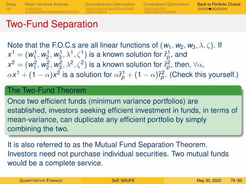
Two-Fund Separation
Note that the F.O.C.s are all linear functions of (w1,w2,w3, λ, ζ). Ifx1 = (w1
1 ,w12 ,w
13 , λ
1, ζ1) is a known solution for r1p , and
x2 = (w21 ,w
22 ,w
23 , λ
2, ζ2) is a known solution for r2p , then, ∀α,
αx1 + (1− α)x2 is a solution for αr1p + (1− α)r2
p . (Check this yourself.)
The Two-Fund TheoremOnce two efficient funds (minimum variance portfolios) areestablished, investors seeking efficient investment in funds, in terms ofmean-variance, can duplicate any efficient portfolio by simplycombining the two.
It is also referred to as the Mutual Fund Separation Theorem.Investors need not purchase individual securities. Two mutual fundswould be a complete service.
QUANTITATIVE FINANCE SoF, SHUFE May 30, 2020 79 / 85
Setup Mean-Variance Analysis Unconstrained Optimization Constrained Optimization Back to Portfolio Choice
Two-Fund Separation - Discussions
The Two-Fund Theorem relies crucially on the following assumptions.1 Investors only care mean and variance.2 Investors have the same assessment of the means, variances and
covariances.3 A single-period investment horizon.
All the three assumptions are tenuous in reality. But the theoremprovides a good way to understand the investment process.� For instance, if investors care more than mean and variance and
invest for multiple periods, the two-fund separation is no longattained. However, we may have a three-fund separation.4
4See Merton, Robert C., 1973. An intertemporal capital asset pricing model,Econometrica 41(5), 867-887. We will not cover it in this course.
QUANTITATIVE FINANCE SoF, SHUFE May 30, 2020 80 / 85
Setup Mean-Variance Analysis Unconstrained Optimization Constrained Optimization Back to Portfolio Choice
Adding a Riskfree Asset
So far we have focused on risky assets with σ > 0.
Introduction of a riskfree asset with σ = 0 enables borrowing andlending at the riskfree rate rf .
Perhaps surprisingly, adding one more riskfree asset causes amathematical degeneracy hence greatly simplifies the shape of theefficient frontier.
For a portfolio with a weight α (α ≤ 1) in the riskfree asset and a weight1− α in a risky asset with mean return of r and standard deviation σ,
rp = αrf + (1− α)r , σp = (1− α)σ.
QUANTITATIVE FINANCE SoF, SHUFE May 30, 2020 81 / 85
Setup Mean-Variance Analysis Unconstrained Optimization Constrained Optimization Back to Portfolio Choice
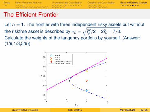
The Efficient Frontier
Let rf = 1. The frontier with three independent risky assets but withoutthe riskfree asset is described by σp =
√r2p /2− 2rp + 7/3.
Calculate the weights of the tangency portfolio by yourself. (Answer:(1/9,1/3,5/9))
QUANTITATIVE FINANCE SoF, SHUFE May 30, 2020 82 / 85
Setup Mean-Variance Analysis Unconstrained Optimization Constrained Optimization Back to Portfolio Choice
The One-Fund TheoremAny efficient portfolio is a combination of riskfree borrowing/lendingand a single fund of risky assets.
Note that on the aggregate level, borrowing and lending cancel out.The weights would be 100% in the risky fund, and 0% in the riskfreeasset.
We are ready to study market equilibrium, for instance, the CapitalAsset Pricing Model.
QUANTITATIVE FINANCE SoF, SHUFE May 30, 2020 83 / 85
Setup Mean-Variance Analysis Unconstrained Optimization Constrained Optimization Back to Portfolio Choice
Question
Question on the Tangency PortfolioWhat are the weights of the tangency portfolio?
QUANTITATIVE FINANCE SoF, SHUFE May 30, 2020 84 / 85
Setup Mean-Variance Analysis Unconstrained Optimization Constrained Optimization Back to Portfolio Choice
Question
Question on the Tangency PortfolioWhat are the weights of the tangency portfolio?
The frontier of risky assets is the curve σ2p = r2
p /2− 2rp + 7/3.Differentiate both sides, we obtain:
2σpdσp = rpdrp − 2drp, =⇒drp
dσp=
2σp
rp − 2
The slope of the tangency line is rp−rfσp
. Let the two slopes equal.
=⇒ rp =14/3− 2rf
2− rf.
Then w1 = 1/3− (rp/2− 1),w2 = 1/3,w3 = 1/3 + (rp/2− 1).
QUANTITATIVE FINANCE SoF, SHUFE May 30, 2020 85 / 85