Embed Size (px)
Citation preview
QUANTITATIVE FINANCE RESEARCH CENTRE QUANTITATIVE F
INANCE RESEARCH CENTRE
QUANTITATIVE FINANCE RESEARCH CENTRE
Research Paper 264 December 2009
Simulation of Diversified Portfolios in a Continuous Financial Market
Eckhard Platen and Renata Rendek
ISSN 1441-8010 www.qfrc.uts.edu.au

Simulation of
Diversified Portfolios in
a Continuous Financial Market
Eckhard Platen 1 and Renata Rendek1
December 1, 2009
Abstract. In this paper we analyze the simulated behavior of diversifiedportfolios in a continuous financial market. In particular, we focus on equallyweighted portfolios. We illustrate that these well diversified portfolios con-stitute good proxies of the growth optimal portfolio. The multi-asset marketmodels considered include the Black-Scholes model, the Heston model, theARCH diffusion model, the geometric Ornstein-Uhlenbeck volatility modeland the multi-currency minimal market model. The choice of these modelswas motivated by the fact that they can be simulated almost exactly and,therefore, very accurately also over longer periods of time. Finally, we pro-vide examples, which demonstrate the robustness of the diversification phe-nomenon when approximating the growth optimal portfolio of a market byan equal value weighted portfolio. Significant outperformance of the marketcapitalization weighted portfolio by the equal value weighted portfolio can beobserved for models.
2000 Mathematics Subject Classification: 91B28, 62P05, 62P20
Key words and phrases: Growth optimal portfolio, Diversification Theorem, di-versified portfolios, equally weighted portfolio, exact simulation.
1University of Technology Sydney, School of Finance & Economics and Department of
Mathematical Sciences, PO Box 123, Broadway, NSW, 2007, Australia

1 Introduction
Diversification is a concept that has been successfully applied for centuries. Whenconstructing a diversified portfolio (DP) the proportion of the value of the hold-ing in any individual security, relative to the total portfolio value, convergessufficiently fast to zero as the number of securities increases. In the literature re-lated to portfolio optimization DPs play a significant role, see Karatzas & Shreve(1998). Their asymptotic properties have been analyzed by Bjork & Naslund(1998), Hofmann & Platen (2000), Platen (2004a) and Guan, Liu & Chong (2004).Additionally, a notion of diversification in a particular modern portfolio sense canbe found in Fernholz (2002).
We consider DPs under the benchmark approach described in Platen (2002) and(2004b). This concept is related to the notion of a growth optimal portfolio
(GOP). The GOP is defined as the portfolio that maximizes expected logarithmicutility from terminal wealth, see Kelly (1956). The GOP is the best performingportfolio in the long run and can be used in derivative pricing, risk managementand portfolio optimization. It appears in a wide range of literature including,for instance, Long (1990), Artzner (1997), Bajeux-Besnainou & Portait (1997),Karatzas & Shreve (1998), Kramkov & Schachermayer (1999), Becherer (2001),Platen (2002) and Goll & Kallsen (2003).
In practice, it is difficult to construct proxies of the GOP based on estimatesof risk premia. It is, in principle, not possible to estimate any drift parameterwith sufficient significance to be useful in sample based portfolio optimization,see Fama & French (2003) and DeMiguel, Garlappi & Uppal (2009). However,the Diversification Theorem proved in Platen (2005), shows that for a sequenceof regular jump diffusion financial markets, any sequence of DPs is a sequence ofapproximate GOPs. This allows one in practice to approximate the GOP by anywell diversified global market index.
This paper aims to demonstrate the robustness of the Diversification Theorem bysimulating the GOP and DPs under various continuous financial market models.We emphasize that these simulations are exact or almost exact. The only approx-imation we allow is the approximation of integrals with respect to functions offinite variation. This avoids typical problems of stochastic numerical simulationas questions related to the non-Lipschitzness of coefficients, numerical stabilityand potential negative values for positive processes, propagation of errors, etc..By focusing on almost exact simulations we make our results much more reli-able than is typically achieved when using discrete time approximations of SDEsbased on various schemes. The simulation results presented here give an impres-sion about the closeness of DPs to the GOP when these are constructed from realmarket data, see, for instance, Platen & Rendek (2008).
We will simulate asset prices with dynamics modeled by the multi-asset Black-Scholes model, see Black & Scholes (1973); the multi-asset Heston model, see
2

Heston (1993); the multi-asset ARCH-diffusion model, see Nelson (1990) andFrey (1997); the multi-asset geometric Ornstein-Uhlenbeck volatility model, seeWiggins (1987) or Follmer & Schweizer (1993); and the multi-currency minimalmarket model, see Platen (2001). These examples will illustrate the robustness ofthe diversification effect. The simulation studies will confirm that the convergencebehavior of DPs towards the GOP appears to be largely model independent. Thisprovides an important robustness property for applications of the benchmark ap-proach. Finally, the paper makes the observation that for models, where theprimary security accounts when expressed in units of the GOP are strict super-martingales, a well diversified portfolio, like the equal value weighted portfolio,significantly outperforms the typical market portfolio in the long run.
This paper is structured as follows. Section 2 defines DPs in a continuous financialmarket. Sections 3-8 describe exact or almost exact simulation of continuousfinancial market models. These sections also include simulation study of DPsunder various model dynamics. In Section 3 we consider the multi-asset Black-Scholes model dynamics; in Section 4 the multi-asset Heston model dynamics;in Section 5 the multi-asset ARCH diffusion model dynamics; in Section 6 themulti-asset geometric Ornstein-Uhlenbek volatility model dynamics; in Section 7the multi-currency minimal market model; and, finally, in Section 8 the multi-currency generalized minimal market model dynamics. Section 9 concludes.
2 Diversified Portfolios
Given a filtered probability space (Ω,A,A, P ), where A = (At)t∈[0,∞) is the fil-tration which satisfies the usual conditions, we consider markets with continuoussecurity prices. Trading uncertainty is modeled by independent standard (A, P )-Wiener processes W k = W k
t , t ∈ [0,∞), for k ∈ 1, 2, . . . , d and d ∈ 1, 2, . . ..We consider a sequence of continuous financial market (CFM) models SC
(d) indexed
by a number d ∈ 1, 2, . . .. For given d the corresponding CFM comprises d + 1primary security accounts, denoted by S0
(d), S1(d), . . . , S
d(d). These include a savings
account S0(d) = S0
(d)(t), t ∈ [0,∞), which is the locally riskless primary securityaccount expressed by
S0(d)(t) = exp
∫ t
0
rsds
< ∞ (2.1)
for t ∈ [0,∞), where r = rt, t ∈ [0,∞) denotes the adapted short rate.
As shown in Platen & Heath (2006), in the dth CFM SC(d) there exists a unique
GOP Sδ∗(d) = Sδ∗
(d)(t), t ∈ [0,∞). The dth GOP is a strictly positive portfolio that
maximizes the expected log-utility from terminal wealth, that is E(
ln(
Sδ(d)(T )
))
for any T ∈ [0,∞), over all strictly positive portfolios Sδ(d) for d ∈ 1, 2, . . .,
3
see Kelly (1956). It is a central object in the dth financial market SC(d) with
outstanding mathematical properties.
In particular, one can use the GOP as benchmark. Let us, therefore, define the jthsequence of benchmarked primary security account processes Sj
(d) = Sj
(d)(t), t ∈[0,∞) by the ratio
Sj
(d)(t) =Sj
(d)(t)
Sδ∗(d)(t)
(2.2)
for t ∈ [0,∞) and j ∈ 0, 1, . . . , d, d ∈ 1, 2, . . ..We also define a benchmarked portfolio process Sδ
(d) = Sδ(d)(t), t ∈ [0,∞) in
SC(d), where its value at time t is given by
Sδ(d)(t) =
d∑
j=0
δjt S
j
(d)(t). (2.3)
The self-financing property of this portfolio is visible in the form of the followingstochastic differential equation (SDE)
dSδ(d)(t) =
d∑
j=0
δjt dSj
(d)(t) (2.4)
for t ∈ [0,∞). Here, the vector of process of the predictable number of units in-vested δ = δt = (δ0
t , δ1t , . . . , δ
dt )
⊤, t ∈ ℜ+ represents the corresponding strategy,if the Ito integral
∫ t
0
δjsdSj
(d)(s) (2.5)
exists for all j ∈ 0, 1, . . . , d, d ∈ 1, 2, . . . and t ∈ [0,∞).
All strategies and portfolios we will consider are self-financing. Moreover, sinceself-financing portfolios can, in general, become zero or negative in value, weconsider in the following portfolios which are strictly positive.
Furthermore, we define for SC(d) the fraction πj
δ,t of Sδ(d)(t) that is invested in the
jth benchmarked primary security account Sj
(d)(t), j ∈ 1, 2, . . . , d, at time t,which is given by the formula
πjδ,t = δj
t
Sj
(d)(t)
Sδ(d)(t)
(2.6)
for j ∈ 1, 2, . . . , d. Note that fractions can be negative but always sum to one,that is
d∑
j=0
πjδ,t = 1 (2.7)
4

for t ∈ [0,∞).
Let us now describe potential proxies for the GOP. For a sequence of CFMs(
SC(d)
)
d∈1,2,... we call a corresponding sequence
(
Sδ(d)
)
d∈1,2,... of strictly positive
portfolio processes Sδ(d) a sequence of diversified portfolios (DPs) if some constants
K1, K2 ∈ (0,∞) and K3 ∈ 1, 2, . . . exist, independently of d, such that ford ∈ K3, K3 + 1, . . . the inequality
|πjδ,t| ≤
K2
d1
2+K1
(2.8)
holds almost surely for all j ∈ 0, 1, . . . , d and t ∈ [0,∞). This means that fora DP the fractions decline sufficiently fast for increasing d but need not to beequal.
We need to assume that in a given sequence of CFMs the primary security ac-counts are sufficiently different. Otherwise, one cannot expect that any diversi-fication is possible in the market under consideration. To achieve a sufficientlyregular market let us ensure that each of the independent sources of tradinguncertainty influences only a restricted range of benchmarked primary securityaccounts. More precisely, we assume the following regularity condition:
E(
(σk(d)(t))
2)
≤ K5 (2.9)
for all t ∈ [0,∞), d ∈ 1, 2, . . ., k ∈ 1, 2, . . . , d and a constant K5 ∈ (0,∞).Here σk
(d)(t) is referred to as the k-th total specific volatility for SC(d) and is defined
by the sum
σk(d)(t) =
d∑
j=0
|σj,k
(d)(t)| (2.10)
for k ∈ 1, 2, . . .. The (j, k)th specific volatility σj,k
(d), is the volatility of the jthbenchmarked primary security account with respect to the kth source of tradinguncertainty, see Platen & Heath (2006).
Furthermore, to measure the distance between an approximating portfolio Sδ(d)
and the GOP Sδ∗(d) we define the tracking rate Rδ
(d)(t) at time t by
Rδ(d)(t) =
d∑
k=1
(
d∑
j=0
πjδ,tσ
j,k
(d)(t)
)2
(2.11)
for t ∈ [0,∞). Note that one can show that the tracking rate vanishes when Sδ(d)
equals Sδ∗(d). This is simply the consequence of the fact that the benchmarked
GOP is a constant and, thus, has zero returns.
For a sequence(
SC(d)
)
d∈1,2,... of CFMs a sequence of strictly positive portfolios
(
Sδ(d)
)
d∈1,2,... is called a sequence of approximate GOPs when the corresponding
5

sequence of tracking rates vanishes in probability, that is
limd→∞
Rδ(d)(t) = 0 (2.12)
for all t ∈ [0,∞).
In reality one observes that well diversified, global stock portfolios behave verysimilar. This can be mathematically verified without imposing any major mod-eling assumptions. The Diversification Theorem proved in Platen (2005), showsthat for a regular sequence of CFMs, see (2.9), any sequence of DPs is a sequenceof approximate GOPs. Moreover, for any d ∈ K3, K3 + 1, . . . and t ∈ [0,∞),the expected tracking rate of a given DP can be shown to satisfy the estimate
E(
Rδ(d)(t)
)
≤ (K2)2K5
d2K1. (2.13)
Here, K1, K2, K5 ∈ (0,∞) and K3 ∈ 1, 2, . . ..This theorem is similar to the Law of Large Numbers and of practical significance.It allows us to approximate the GOP by any diversified global market index. Itis very important to note that this result is model independent. It states thatapproximation of the GOP can be achieved by avoiding any calculation of theexact theoretical GOP fractions. This allows to overcome in practice the problemof risk premia which is, in principle, not possible with sufficient significance tobe useful in portfolio optimization, see Fama & French (2003) and DeMiguel,Garlappi & Uppal (2009). By the Diversification Theorem one obtains proxiesfor the GOP in a robust manner as will be discussed in Sections 3-8.
In the following sections we illustrate the robustness of the diversification effectby simulation of diversified portfolios for various market models. By exploitingthe nature of the market dynamics considered the simulation will be performedexactly or almost exactly. This is highly important since we want to study thediversification phenomenon over long periods of time.
To keep the presentation simple and transparent we consider in this paper onlytwo types of indices, market capitalization weighted indices (MCIs) and equally
weighted indices (EWIs). The indices constructed in this study are all self-financing portfolios. We characterize the indices in terms of fractions as in (2.6).For an MCI we define the fraction of wealth held in the jth constituent at timetn by the ratio
πjδMCI ,tn
=δjMCI,tn
Sjtn
∑d
i=1 δiMCI,tn
Sitn
, (2.14)
for j ∈ 1, 2, . . . , d, where δjMCI,tn
denotes the number of units of the jth con-stituent available in the market at time tn. An equally weighted index EWI isobtained by setting all fractions equal at the beginning of each trading period.The jth fraction of an EWI is then simply given by the constant ratio
πjδEWI ,tn
=1
d(2.15)
6

for j = 1, 2, . . . , d. Given the respective fractions, the value of a portfolio attime tn is recursively obtained according to the relation
Sδtn
= Sδtn−1
(
1 +d∑
j=1
πjδ,tn−1
Sjtn − Sj
tn−1
Sjtn−1
)
(2.16)
or equivalently
Sδtn
= Sδtn−1
+
d∑
j=1
δjtn−1
(
Sjtn − Sj
tn−1
)
. (2.17)
According to a given marked dynamics we simulate for the long period of T = 150years the benchmarked trajectories of d + 1 = 1001 primary security accounts,sampling twice a week. For simplicity we set the interest rate to zero. Thus, theinverse of the benchmarked savings account provides the GOP when denominatedin domestic currency, that is
Sδ∗t = (S0
t )−1. (2.18)
The product of the GOP with the jth benchmarked primary security accountyields the value of the jth primary security account denominated in domesticcurrency, that is,
Sjt = Sj
t Sδ∗t , (2.19)
for j ∈ 0, 1, . . . , d. The initial values Sj0, j ∈ 0, 1, . . . , d, are generated ac-
cording to a Pareto distribution with parameters λ = 1.1 and x0 = λ−1λ
, seeSimon (1958). For each model we plot the first 20 benchmarked primary securityaccount processes in the respective figures in Sections 3-8. We also give an im-pression about the typical squared volatility process in these sections. Moreover,we plot for each market dynamics the simulated GOP as well as the EWI and theMCI, constructed from the simulated primary security accounts as described in(2.19). Additionally, we display in a separate figure for each market dynamics thebenchmarked EWI and the benchmarked MCI. The benchmarked GOP is simplythe constant one.
3 Multi-asset Black-Scholes Model
In this paper we use exact or almost exact simulation techniques for solutions ofSDEs. When using discrete time numerical schemes for simulation there may beissues when dealing with non-Lipschitz continuous drift or diffusion coefficients.Also problems concerning numerical stability may arise or negative values couldbe obtained for strictly positive processes. Therefore, we describe in the followingsections methods of exact and almost exact simulation of various market models,which avoid in principle, most of these problems. For simplicity, this presentationdescribes simulation methods for independent benchmarked primary security ac-counts. However, the case of dependent benchmarked primary security accounts
7

0 50 100 1500
2
4
6
8
10
12
Figure 3.1: Simulated benchmarked primary security accounts under the Black-Scholes model
can be handled analogously. For details on simulation of correlated assets werefer to Platen & Rendek (2009).
Let us first describe the standard market model, which is the multi-asset Black-Scholes model, see Black & Scholes (1973). Under this model the benchmarkedprimary security accounts can be represented by the following matrix SDE
dSt =
d∑
k=1
BkStdW k
t , (3.1)
for t ∈ [0,∞). Here S = St = (S0t , S
1t , . . . , S
dt )
⊤, t ∈ [0,∞) is a vector ofbenchmarked primary security accounts, and B
k = [Bk,i,j]di,j=1 is a d×d diagonalparameter matrix, with elements
Bk,i,j = bj,k for i = j
0 otherwise(3.2)
for k, i, j ∈ 1, 2, . . . , d. Note that Sj, j ∈ 1, 2, . . . , d forms here a martingale.
The multi-asset Black-Scholes model can be simulated exactly. The matrix SDE(3.1) has an exact solution, see Platen & Heath (2006). The jth benchmarkedprimary security accounts can be represented by
Sjt = Sj
0 exp
− 1
2
d∑
k=1
(
bj,k)2
t +
d∑
k=1
bj,kW kt
. (3.3)
Therefore, for the time discretization 0 < t0 < t1 < · · · < ∞, where ti = ∆i,
8

0 50 100 1500
100
200
300
400
500
600
GOP
EWI
MCI
Figure 3.2: Simulated GOP, EWI and MCI under the Black-Scholes model
0 50 100 1500.55
0.6
0.65
0.7
0.75
0.8
0.85
0.9
0.95
1
1.05
benchmarked MCI
benchmarked EWI
Figure 3.3: Simulated benchmarked GOP, EWI and MCI under the Black-Scholesmodel
i ∈ 0, 1, . . ., we obtain the exponential
Sjti+1
= Sj0 exp
− 1
2
(
bj,j)2
ti+1 + bj,jW jti+1
(3.4)
for the jth independent benchmarked primary security account under the Black-Scholes model.
Let us now illustrate the fundamental phenomenon of diversification by simu-lating in a Black-Scholes market diversified portfolios. This can be exactly per-
9

formed without any error as described above. We simulate 1001 independentbenchmarked primary security accounts with bj,j = 0.2 for j ∈ 0, 1, . . . , 1000according to (3.4) end display the first 20 resulting trajectories in Fig.3.1. We em-phasize that these benchmarked primary security accounts are here martingales.Here, the independent initial value Sj
0 is generated using the Pareto distributionwith parameters λ = 1.1 and x0 = λ−1
λ, see Simon (1958). This models the fact
that there is a great variety in the market capitalization of stocks.
In Fig 3.2 we show the simulated GOP, the EWI and the MCI. In this case theEWI approximates rather well the GOP. The MCI seems to be initially a goodproxy of the GOP, however after this initial time period it diverges from the GOP.Most likely some large stock values emerge and the resulting large fractions ofthese stocks distort the performance of the market index. These fractions of thecorresponding primary security accounts are simply to large to be acceptable asthose of a DP and, thus violate the conditions of the Diversification Theorem.This phenomenon is also illustrated in Fig.3.3 where we display the benchmarkedGOP, Sδ∗
t = 1, as well as the benchmarked EWI simulated under the Black-Scholes model and the benchmarked MCI constructed from 1000 benchmarkedprimary security accounts. Note that initially in the first 10 years, sometimes thebenchmarked EWI, sometimes the benchmarked MCI performed better. However,in the long term simulation we clearly see that the benchmarked EWI convergesin the long run to the benchmarked GOP, while the benchmarked MCI tendsdownwards. In this figure we also note that the benchmarked MCI has muchlarger variance then the benchmarked EWI.
4 Multi-asset Heston Model
The Heston model, see Heston (1993), can be described by a set of two matrixSDEs in the form
dSt = diag(
√
V t
)
diag(
St
)(
AdW1
t + BdW2
t
)
, (4.1)
dV t = (a − EV t) dt + F diag(√
V t
)
dW1
t , (4.2)
for t ∈ [0,∞). Here S = St = (S0t , S
1t , . . . , S
dt )
⊤, t ∈ [0,∞) is a vector ofbenchmarked primary security accounts which are supermartingales, see Platen
& Heath (2006). Moreover, W1
= W 1
t = (W 1,1t , W 1,2
t , . . . , W 1,dt )⊤, t ∈ [0,∞)
and W2
= W 2
t = (W 2,1t , W 2,2
t , . . . , W 2,dt )⊤, t ∈ [0,∞) are independent vectors
of correlated Wiener processes. That is
Wk
t = CkW
kt , (4.3)
where Ck = [Ck,i,j]di,j=1 and W
k = W kt = (W k,1
t , W k,2t , . . . , W k,d
t )⊤, t ∈ [0,∞),k ∈ 1, 2 is again a vector of independent Wiener processes.
10

0 50 100 1500
0.2
0.4
0.6
0.8
1
1.2
1.4
1.6
1.8
Figure 4.1: Simulated benchmarked primary security accounts under the Hestonmodel
Additionally, A = [Ai,j ]di,j=1 is a diagonal matrix with elements
Ai,j =
i for i = j0 otherwise
(4.4)
and B = [Bi,j]di,j=1 is a diagonal matrix with elements
Bi,j =
√
1 − 2i for i = j
0 otherwise.(4.5)
Moreover, V = V t = (V 1t , V 2
t , . . . , V dt )⊤, t ∈ [0,∞) is a vector of squared
volatilities, a = (a1, a2, . . . , ad)⊤; and E = [Ei,j]di,j=1 is a diagonal matrix with
elements
Ei,j = κi for i = j
0 otherwise,(4.6)
and F = [F i,j]di,j=1 is a diagonal matrix with elements
F i,j =
γi for i = j0 otherwise.
(4.7)
One method for the exact simulation of the Heston model has been discussed inBroadie & Kaya (2006). We use here a simplified almost exact simulation of thebenchmarked primary security accounts under the Heston model. This methodinvolves exact simulation of the squared volatility processes and almost exactsimulation of the independent benchmarked primary security accounts, given thetrajectories of the squared volatilities as explained in Platen & Rendek (2009).
11

0 50 100 1500
0.05
0.1
0.15
0.2
0.25
0.3
0.35
0.4
Figure 4.2: Simulated squared volatility under the Heston model
We obtain the value of the jth squared volatility V jti+1
at time ti+1, i ∈ 0, 1, . . .,by sampling directly from the noncentral chi-square distribution χ
′2νj
(λj) with νj
degrees of freedom and noncentrality parameter λj . That is
V jti+1
=γ2
j (1 − exp−κj∆)4κj
χ′2νj
(
4κje−κj∆
γ2j (1 − e−κj∆)
V jti
)
, (4.8)
where νj =4aj
γ2j
. Sampling from the noncentral chi-square distribution is discussed,
for instance, in Glasserman (2004). The resulting simulation method for V j isexact.
Let us now describe the almost exact simulation of the vector of logarithms ofthe benchmarked assets X t = ln(St). Following Broadie & Kaya (2006) we mayrepresent the jth value of Xj
ti+1at time ti+1 in the form
Xjti+1
= Xjti
+j
γj
(
V jti+1
− V jti− aj∆
)
+
(
jκj
γj
− 1
2
)∫ ti+1
ti
V ju du (4.9)
+√
1 − 2j
∫ ti+1
ti
√
V ju dW 2,j
u .
Furthermore, the distribution of
∫ ti+1
ti
√
V ju dW 2,j
u , (4.10)
given the path of V j, is Gaussian with mean zero and variance∫ ti+1
tiV j
u du, since V j
is independent of the Brownian motion W 2,j for all j ∈ 1, 2, . . . , d. Moreover,
12

0 50 100 1500
100
200
300
400
500
600
700
800
900
1000
GOP
EWI
MCI
Figure 4.3: Simulated GOP, EWI and MCI under the Heston model
0 50 100 1500.4
0.5
0.6
0.7
0.8
0.9
1
1.1
benchmarked MCI
benchmarked EWI
Figure 4.4: Simulated benchmarked GOP, EWI and MCI under the Heston model
it is possible to approximate∫ ti+1
tiV j
u du given the path of the process V j. We usehere the well known trapezoidal rule
∫ ti+1
ti
V ju du ≈ ∆
2
(
V jti
+ V jti+1
)
. (4.11)
Consequently,
∫ ti+1
ti
√
V ju dW 2,j
u ≈ N(
0,∆
2
(
V jti
+ V jti+1
)
)
. (4.12)
13

This approximation can be achieved with high accuracy, by the above quadratureformula. For the multi-asset Heston model this results in an efficient almost exactsimulation technique by conditioning.
We now use for the benchmarked primary security accounts the multi-asset Hes-ton model with independent prices. We display the first 20 simulated independentbenchmarked primary security accounts under the multi-asset Hestion model inFig. 4.1. These benchmarked primary security accounts are supermartingales.The parameters in (4.8) are estimated by a Heston fit to the SPX surface as ofthe close on Sep 15, 2005, see Gatheral (2006). The jth squared volatility pro-cess is simulated according to (4.8) for initial value V j
0 = 0.0174, aj = 0.0469,κj = 1.3253, γj = 0.3877, j ∈ 0, 1, . . . , 1000. The correlation parameter is hereset to j = −0.7165 in order to reflect the leverage effect, see Black (1976). The
initial values Sj0 are again generated from the Pareto distribution. Additionally,
we display in Fig. 4.2 a typical trajectory of the squared volatility process V j
under the Heston model simulated exactly with the formula (4.8).
In Fig 4.3 we display the simulated GOP, EWI and MCI under the Heston model.Also here the EWI provides a good proxy for the GOP. The MCI however, doesnot perform as good as the GOP and the EWI. Additionally, in Fig. 4.4 weillustrate the benchmarked GOP, Sδ∗
t = 1, the benchmarked EWI and the bench-marked MCI obtained from 1000 benchmarked primary security accounts. Thisplot clearly shows the convergence of the benchmarked EWI to the benchmarkedGOP. The benchmarked MCI, similar to the simulation under the Black-Scholesmodel, has downward trend.
5 Multi-asset ARCH-diffusion Model
The continuous time limits of some popular time series models in finance canbe described by a multi-dimensional ARCH-diffusion model. The class of ARCHand GARCH time series models was originally proposed in Engle (1982). TheARCH diffusion model is obtained as a continuous time limit of the innovationprocess of the GARCH(1, 1) and NGARCH(1, 1) models, see Nelson (1990) andFrey (1997). The ARCH-diffusion model can be described by the following set oftwo matrix SDEs in the form
dSt = diag(
√
V t
)
diag(
St
)(
AdW1
t + BdW2
t
)
, (5.1)
dV t = (a − EV t) dt + F diag (V t) dW1
t , (5.2)
for t ∈ [0,∞). Here S = St = (S0t , S
1t , . . . , S
dt )
⊤, t ∈ [0,∞) denotes againa vector of benchmarked primary security accounts which are supermartingales.
Furthermore, W1
= W 1
t = (W 1,1t , W 1,2
t , . . . , W 1,dt )⊤, t ∈ [0,∞) and W
2=
W 2
t = (W 2,1t , W 2,2
t , . . . , W 2,dt )⊤, t ∈ [0,∞) are independent vectors of correlated
Wiener processes. Additionally, A = [Ai,j]di,j=1 is a diagonal matrix with elements
14

0 50 100 1500
5
10
15
20
25
30
Figure 5.1: Simulated benchmarked primary security accounts under the ARCH-diffusion model
as in (4.4), and B = [Bi,j]di,j=1 is a diagonal matrix with elements (4.5). Moreover,V = V t = (V 1
t , V 2t , . . . , V d
t )⊤, t ∈ [0,∞) is a vector of squared volatilities,a = (a1, a2, . . . , ad)
⊤; E = [Ei,j]di,j=1 is a diagonal matrix with elements as in(4.6); and F = [F i,j]di,j=1 is a diagonal matrix with elements as in (4.7).
In the given case we can simulate the jth squared volatility process V j, j ∈0, 1, . . . almost exactly by approximating the time integral via the trapezoidalrule in the following exact representation
V jti+1
= exp
(
−κj −1
2γ2
j
)
ti+1 + γjW1,jti+1
(5.3)
×(
V jt0
+ aj
i∑
k=0
∫ tk+1
tk
exp
(
κj +1
2γ2
j
)
s − γjW1,js
ds
)
.
This yields the approximation
V j∆ti+1
= exp
(
−κj −1
2γ2
j
)
ti+1 + γjW1,jti+1
(5.4)
×(
V jt0
+ aj
∆
2
i∑
k=0
[
exp
(
κj +1
2γ2
j
)
tk − γjW1,jtk
+ exp
(
κj +1
2γ2
j
)
tk+1 − γjW1,jtk+1
])
for ti = ∆i, i ∈ 0, 1, . . ..
Let us now describe the almost exact simulation of the vector Xt = ln(
St
)
.
Following Platen & Rendek (2009), we may represent the jth value of Xjti+1
at
15

0 50 100 1500
0.05
0.1
0.15
0.2
0.25
0.3
0.35
0.4
Figure 5.2: Simulated squared volatility under the ARCH-diffusion model
time ti+1 in the following way:
Xjti+1
= Xjti− 1
2
∫ ti+1
ti
V ju du +
2j
γj
(
√
V jti+1
−√
V jti
)
(5.5)
−2j
γj
∫ ti+1
ti
(
aj
2√
V ju
−(
κj
2+
γ2j
8
)√
V ju
)
du
+√
1 − 2j
∫ ti+1
ti
√
V ju dW 2,j
u .
Furthermore, the distribution of
∫ ti+1
ti
√
V ju dW 2,j
u , (5.6)
conditioned on the path of V j , is Gaussian with mean zero and variance∫ ti+1
tiV j
u du,
because V j is independent of the Brownian motion W 2,j for all j ∈ 1, 2, . . . , d.Moreover, it is possible to approximate
∫ ti+1
tiV j
u du given the path of the process
V j . We use here the following trapezoidal approximation
∫ ti+1
ti
V ju du ≈ ∆
2
(
V jti
+ V jti+1
)
(5.7)
to obtain∫ ti+1
ti
√
V ju dW 2,j
u ≈ N(
0,∆
2
(
V jti
+ V jti+1
)
)
. (5.8)
16

0 50 100 1500
100
200
300
400
500
600
700
800
900
1000
EWI
GOP
MCI
Figure 5.3: Simulated GOP, EWI and MCI under the ARCH-diffusion model
0 50 100 150
0.4
0.5
0.6
0.7
0.8
0.9
1
1.1
1.2
1.3
benchmarked EWI
benchmarked MCI
Figure 5.4: Simulated benchmarked GOP, EWI and MCI under the ARCH-diffusion model
Similarly, it is possible to approximate the integral in the form
∫ ti+1
ti
(
aj
2√
V ju
−(
κj
2+
γ2j
8
)√
V ju
)
du ≈ (5.9)
∆
2
aj
2√
V jti
−(
κj
2+
γ2j
8
)
√
V jti
+aj
2√
V jti+1
−(
κj
2+
γ2j
8
)
√
V jti+1
.
This approximation can be achieved with high accuracy by using the simple
17

0 50 100 1500
0.5
1
1.5
Figure 6.1: Simulated benchmarked primary security accounts under the geomet-ric Ornstein-Uhlenbeck volatility model
quadrature formula. We obtain an efficient almost exact simulation technique byconditioning for the multi-asset ARCH-diffusion model.
Let us now simulate the benchmarked primary security accounts as a multi-dimensional ARCH diffusion, as described above. We make the squared volatilityprocess the same for all benchmarked primary security accounts, where we seta = 0.0469, κ = 1.3253, γ = 1 and V0 = 0.0174, as calibrated by comparisonto the Heston squared volatility process. Furthermore, the driving noise of eachof the benchmarked asset prices is independent from each other. It is, however,correlated with = −0.7165 to the corresponding squared volatility process.In Fig. 5.1 we show the first 20 resulting benchmarked risky primary securityaccounts. A typical trajectory of the squared volatility under the ARCH-diffusionmodel is displayed in Fig. 5.2.
The Fig. 5.3 display the corresponding GOP, EWI and MCI. Moreover, Fig. 5.4exhibits the benchmarked GOP, Sδ∗
t = 1, the benchmarked EWI and the bench-marked MCI. Also here the EWI appears to be a very good proxy of the GOP,while the MCI does not come close enough to the GOP to be acceptable as agood proxy.
18

0 50 100 1500
0.05
0.1
0.15
0.2
0.25
0.3
0.35
0.4
0.45
Figure 6.2: Simulated squared volatility under the geometric Ornstein-Uhlenbeckvolatility model
6 Geometric Ornstein-Uhlenbeck Volatility
Model
Similar as in the Heston and the ARCH-diffusion model we generate the bench-marked asset prices by using some stochastic volatility that is now a geometricOrnstein-Uhlenbeck process. The geometric Ornstein-Uhlenbeck volatility modelcan be described by the following set of two matrix SDEs in the form
dSt = diag (expV t) diag(
St
)(
AdW1
t + BdW2
t
)
, (6.1)
dV t = (a − EV t) dt + F dW1
t , (6.2)
for t ∈ [0,∞). Here S = St = (S0t , S
1t , . . . , S
dt )
⊤, t ∈ [0,∞) denotes againa vector of benchmarked primary security accounts which are supermartingales.
Furthermore, W1
= W 1
t = (W 1,1t , W 1,2
t , . . . , W 1,dt )⊤, t ∈ [0,∞) and W
2=
W 2
t = (W 2,1t , W 2,2
t , . . . , W 2,dt )⊤, t ∈ [0,∞) are independent vectors of correlated
Wiener processes. Additionally, A = [Ai,j]di,j=1 is a diagonal matrix with elementsas in (4.4), and B = [Bi,j]di,j=1 is a diagonal matrix with elements (4.5). Moreover,
expV =
expV t =(
expV 1t , expV 2
t , . . . , expV dt )⊤
, t ∈ [0,∞)
(6.3)
is a vector of volatilities, whose elements are correlated exponents of the Ornstein-Uhlenbeck processes. Additionally a = (a1, a2, . . . , ad)
⊤; E = [Ei,j]di,j=1 is adiagonal matrix with elements as in (4.6); and F = [F i,j]di,j=1 is a diagonal matrixwith elements as in (4.7).
19

0 50 100 1500
100
200
300
400
500
600
700
800
900
GOP
EWI
MCI
Figure 6.3: Simulated GOP, EWI and MCI under the geometric Ornstein-Uhlenbeck volatility model
0 50 100 1500.4
0.5
0.6
0.7
0.8
0.9
1
1.1
1.2
1.3
1.4
benchmarked EWI
benchmarked MCI
Figure 6.4: Simulated benchmarked GOP, EWI and MCI under the geometricOrnstein-Uhlenbeck volatility model
As before we consider simulation of independent benchmarked primary securityaccounts. We obtain the value of the jth volatility exp
V jti
at time ti, i ∈0, 1, . . ., by the following exact solution
expV jti = exp
V j0 e−κjti +
aj
κj
(
1 − e−κjti)
+ γje−κjti
i∑
k=1
∫ tk
tk−1
eκjsdW 1,js
.
(6.4)
20

Here∫ tk
tk−1
eκjsdW 1,js ∼ N
(
0,1
2κ
(
e2κjtk − e2κjtk−1
)
)
. (6.5)
The resulting simulation method for expV j is exact.
Let us now describe the almost exact simulation of the vector Xt = ln(
St
)
.
Again, following Platen & Rendek (2009), we may represent the jth value ofXj
ti+1at time ti+1 in the following way:
Xjti+1
= Xjti− 1
2
∫ ti+1
ti
e2Vju du +
j
γj
(
eV
jti+1 − eV
jti
)
(6.6)
−j
γj
∫ ti+1
ti
((
aj +γ2
j
2
)
eVju − κjV
ju eV
ju
)
du
+√
1 − 2j
∫ ti+1
ti
eVju dW 2,j
u .
Furthermore, the distribution of
∫ ti+1
ti
eVju dW 2,j
u , (6.7)
conditioned on the path of V j , is Gaussian with mean zero and variance∫ ti+1
tie2V
ju du,
because V j is independent of the Brownian motion W 2,j for all j ∈ 1, 2, . . . , d.Moreover, it is possible to approximate
∫ ti+1
tie2V
ju du given the path of the process
V j . We use here the following trapezoidal approximation
∫ ti+1
ti
e2Vju du ≈ ∆
2
(
e2Vjti + e
2Vjti+1
)
(6.8)
to obtain∫ ti+1
ti
eVju dW 2,j
u ≈ N(
0,∆
2
(
e2Vjti + e
2Vjti+1
)
)
. (6.9)
Similarly, it is possible to approximate the integral in the form
∫ ti+1
ti
((
aj +γ2
j
2
)
eVju − κjV
ju eV
ju
)
du ≈ (6.10)
∆
2
((
aj +γ2
j
2
)
eVjti − κjV
jtieV
jti +
(
aj +γ2
j
2
)
eV
jti+1 − κjV
jti+1
eV
jti+1
)
.
This approximation can be achieved with high accuracy by using the simplequadrature formula. We obtain an efficient almost exact simulation technique byconditioning for the multi-asset geometric Ornstein-Uhlenbeck volatility model.
We now simulate the benchmarked primary security accounts from a multi-dimensional geometric Ornstein-Uhlenbeck volatility model, as described above.
21

0 50 100 1500
2
4
6
8
10
12
Figure 7.1: Simulated benchmarked primary security accounts under the MMM
We make the squared volatility process e2V j
calibrated by comparison to theHeston and the ARCH-diffusion squared volatility processes, where we set aj =−2.2143, κj = 1.3253, γj = 0.52 and V j
0 = −2.0257, j ∈ 0, 1, . . . , 1000. Fur-thermore, the driving noise of each of the benchmarked asset prices is independentfrom each other. It is, however, correlated with j = −0.7165 to the correspondingsquared volatility process. In Fig. 6.1 we show the first 20 resulting benchmarkedrisky primary security accounts. A typical trajectory of the squared volatilityunder the geometric Ornstein-Uhlenbeck model is displayed in Fig. 6.2.
The Fig. 6.3 displays the corresponding GOP, EWI and MCI. Moreover, Fig. 6.4exhibits the benchmarked GOP, Sδ∗
t = 1, the benchmarked EWI and the bench-marked MCI. Also here the EWI appears to be a very good proxy of the GOP.As before the MCI does not come close enough to the GOP to be acceptable asa good proxy.
7 Multi-currency Minimal Market Model
Let us now consider the stylized multi-currency minimal market model (MMM)similar to the version of the MMM described in Platen (2001) and Platen & Heath(2006). This time we model the jth benchmarked primary security account bythe expression
Sjt =
1
Y jt αj
t
, (7.1)
where αjt = αj
0 expηjt, j ∈ 0, 1, . . . , d. Here ηj is the jth net growth rate forj ∈ 0, 1, . . . , d, and Y j
t is the time t value of the square root process Y j , which
22

0 50 100 1500
0.1
0.2
0.3
0.4
0.5
0.6
0.7
0.8
Figure 7.2: Simulated squared volatility under the MMM
satisfies the SDE
dY jt =
(
1 − ηjY jt
)
dt +
√
Y jt dW j
t (7.2)
for t ∈ [0,∞), where we set Y j0 = 1
ηj for j ∈ 0, 1, . . . , d. Here W = W t =
(W 1t , W 2
t , . . . , W dt )⊤, t ∈ [0,∞) is a vector of correlated Wiener processes.
Note also that under the MMM, Sj(ϕj(t)) = Y jt αj
t is a squared Bessel process ofdimension four in the, so called, ϕj-time. That is,
dSj(ϕj(t)) = 4dϕj(t) + 2√
Sj(ϕj(t))dW j(ϕj(t)) (7.3)
for t ∈ [0,∞), where one has
ϕj(t) =αj
0
4ηj
(
expηjt − 1)
(7.4)
and
dW j(ϕj(t)) = dW jt
√
dϕj(t)
dt. (7.5)
The inverse Sj(ϕj(t)) of the jth squared Bessel process of dimension four in ϕj-time is here represented by the following SDE
dSj(ϕj(t)) = −2(
Sj(ϕj(t)))
3
2
dW j(ϕj(t)) (7.6)
for t ∈ [0,∞). It can be shown that Sj is a strict supermartingale, see Protter(2004) and Platen & Heath (2006).
23

0 50 100 15010
−1
100
101
102
103
104
105
106
GOP
EWI
MCI
Figure 7.3: Simulated GOP, EWI and MCI under the MMM model in the log-scale
0 50 100 1500
0.2
0.4
0.6
0.8
1
1.2
1.4
benchmarked MCI
benchmarked EWI
Figure 7.4: Simulated benchmarked GOP, EWI and MCI under the MMM model
Let us now explain the simulation of independent benchmarked primary securityaccounts under the MMM. Given the time discretization 0 < t0 < t1 < . . . , whereti = ∆i, i ∈ 0, 1, . . . we first obtain (7.4) for i ∈ 0, 1, . . . and j ∈ 0, 1, . . . , d.The next step is to simulate for the jth benchmarked primary security accountfour independent Wiener processes W k,j, k ∈ 1, 2, 3, 4 in ϕj time. This can beachieved by simply calculating
W k,jti+1
= W k,jti
+√
ϕj(ti+1) − ϕj(ti)Zki+1, (7.7)
24

where Zki+1 ∼ N (0, 1) is a standard Gaussian random variable. Here k ∈ 1, 2, 3, 4,
j ∈ 0, 1, . . . , d and i ∈ 0, 1, . . ..Then the jth benchmarked primary security account at time ti+1 is simulated bythe expression
Sjti+1
= Sj(
ϕj(ti+1))
=1
∑4k=1
(
wk + W k,jti+1
)2 , (7.8)
where Sj0 =
∑4k=1(w
k)2 and i ∈ 0, 1, . . ..Let us now simulate the benchmarked risky primary security accounts accordingto the MMM. These processes are strict supermartingales. In our simulation weuse the net growth rate ηj = 0.09 and scaling αj
0 = 0.05 for the MMM and plot inFig. 7.1 the first 20 resulting risky benchmarked primary security accounts. Thejth volatility equals under the MMM at time ti the expression Sj
tiαj
ti. In Fig. 7.2
we plot a typical squared volatility under the MMM.
The GOP, EWI and MCI are displayed in Fig 7.3 in log-scale to see the significantgrowth over the time period. The benchmarked GOP, benchmarked EWI andbenchmarked MCI are shown in Fig. 7.4. The EWI represents a good proxy forthe GOP even though the benchmarked primary security accounts are here strictsupermartingales and trend systematically downward, as exhibited in Fig. 7.1.The MCI again does not perform as good as the EWI and the GOP.
8 Multi-currency Generalized Minimal Market
Model (GMMM)
Let us now describe a generalized version of the MMM, which uses some stochasticmarket activity time τj . We model the jth benchmarked primary security accountby the expression
Sjt =
1
Y j(τj(t))αj(τj(t)), (8.9)
where αj(τj(t)) = αj0 expηjτj(t) and
dY j(τj(t)) =(
1 − ηjY j(τj(t)))
dτj(t) +√
Y j(τj(t))dW j(τj(t)) (8.10)
is the SDE of a time transformed square root process, j ∈ 0, 1, . . . , d. Here W
= W (τj(t)) = (W 1(τj(t)), W 2(τj(t)), . . . , Wd(τj(t)))
⊤, t ∈ [0,∞) is a vector ofcorrelated Wiener processes in τj-time. Moreover, we use the jth market activitytime
τj(t) = τj(0) +
∫ t
0
mjsds, (8.11)
25

0 50 100 1500
2
4
6
8
10
12
14
Figure 8.5: Simulated benchmarked primary security accounts under the GMMMmodel
where τj(0) > 0, see Breymann, Kelly & Platen (2005). Here the jth marketactivity process mj is modeled by a linear diffusion process with SDE
dmjt = κj
(
mj − mjt
)
dt + γjmjtdW j
t , (8.12)
for t ∈ [0,∞). Here the W j are correlated Wiener processes in t-time. Note thatthe equation (8.10) can be rewritten for Y j
t in t-time in the following way
dY jt =
(
1 − ηjY jt ))
mjtdt +
√
Y jt mj
tdW jt , (8.13)
for t ∈ [0,∞), where
dW jt =
√
1
mjt
dW j(τj(t)), (8.14)
j ∈ 1, 2, . . . , d.Since under the GMMM the τj-time is stochastic there will be a need for numericalintegration and the simulation method of the GMMM will be only almost exact. Itcan be, however, as accurate as required by making the time step size sufficientlysmall.
Given the time discretization 0 < t0 < t1 < . . . , where ti = ∆i, i ∈ 0, 1, . . ., we
26
0 50 100 1500
0.2
0.4
0.6
0.8
1
1.2
1.4
1.6
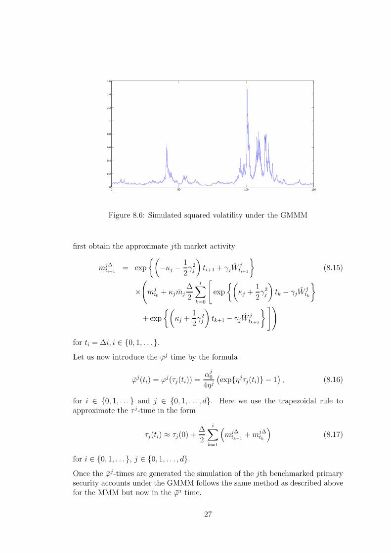
Figure 8.6: Simulated squared volatility under the GMMM
first obtain the approximate jth market activity
mj∆ti+1
= exp
(
−κj −1
2γ2
j
)
ti+1 + γjWjti+1
(8.15)
×(
mjt0
+ κjmj
∆
2
i∑
k=0
[
exp
(
κj +1
2γ2
j
)
tk − γjWjtk
+ exp
(
κj +1
2γ2
j
)
tk+1 − γjWjtk+1
])
for ti = ∆i, i ∈ 0, 1, . . ..Let us now introduce the ϕj time by the formula
ϕj(ti) = ϕj(τj(ti)) =αj
0
4ηj
(
expηjτj(ti) − 1)
, (8.16)
for i ∈ 0, 1, . . . and j ∈ 0, 1, . . . , d. Here we use the trapezoidal rule toapproximate the τ j-time in the form
τj(ti) ≈ τj(0) +∆
2
i∑
k=1
(
mj∆tk−1
+ mj∆tk
)
(8.17)
for i ∈ 0, 1, . . ., j ∈ 0, 1, . . . , d.Once the ϕj-times are generated the simulation of the jth benchmarked primarysecurity accounts under the GMMM follows the same method as described abovefor the MMM but now in the ϕj time.
27

0 50 100 15010
−2
10−1
100
101
102
103
104
105
106
MCI
EWI
GOP
Figure 8.7: Simulated GOP, EWI and MCI under the GMMM model in thelog-scale
0 50 100 1500
0.5
1
1.5
2
2.5
benchmarked EWI
benchmarked MCI
Figure 8.8: Simulated benchmarked GOP, EWI and MCI under the GMMMmodel
As a final model we simulate the multi-currency GMMM. This model generalizesthe MMM by introducing a random market activity time τj . In our simulationwe use one common market time τ defined by the process m with parametersm = 1, κ = 0.1 and γ = 0.1. The net growth rate ηj and the scaling αj
0 are asin the MMM. In Fig. 8.5 we illustrate the resulting benchmarked risky primarysecurity accounts. Under the GMMM the jth squared volatility equal at time tithe product Sj
tiαj
0 expηjτj(ti)mj∆ti
. In Fig.8.6 a typical path of squred volatilityunder the GMMM is exhibited.
28

The GOP, EWI and MCI are displayed in Fig 8.7 in the log-scale. The bench-marked GOP, benchmarked EWI and benchmarked MCI are exhibited in Fig.8.8.Here also the benchmarked primary security accounts are strict supermartingalesand trend downwards in Fig.8.5. This systematic downward trend, however, doesnot destroy the property predicted by the diversification theorem that the EWIconstitutes a good proxy of the GOP when observed over a considerably longtime period. The MCI again does not converge in an acceptable manner to theGOP.
The last two models demonstrated that in the case when the benchmarked pri-mary security accounts are strict supermartingales, the EWI can significantlyoutperform in the long run the MCI. This is an important observation since theMMM appears to be a reasonably realistic market model.
9 Conclusion
We considered in this paper diversified portfolios under various financial marketmodels. All benchmarked primary security accounts under the various multi-assetmodels are supermartingales. The benchmarked primary security accounts of thetwo versions of the multi-currency minimal market model are strict supermartin-gales, which means that these trend systematically downwards. This is also thecase for the typical market capitalization weighted index. It turns out that welldiversified portfolios, such as the equal value weighted index, approximate thegrowth optimal portfolio rather accurately when simulated under all consideredmarket model dynamics. However, for the two versions where benchmarked pri-mary security accounts are strict supermartingales the difference between equalweighted index and market capitalization weighted index is remarkable. This pa-per successfully illustrates the applicability and robustness of the DiversificationTheorem to large markets.
References
Artzner, P. (1997). On the numeraire portfolio. In Mathematics of Derivative
Securities, pp. 53–58. Cambridge University Press.
Bajeux-Besnainou, I. & R. Portait (1997). The numeraire portfolio: A newperspective on financial theory. The European Journal of Finance 3, 291–309.
Becherer, D. (2001). The numeraire portfolio for unbounded semimartingales.Finance Stoch. 5, 327–341.
Bjork, T. & B. Naslund (1998). Diversified portfolios in continuous time. Eu-
ropean Finance Review 1, 361–387.
29

Black, F. (1976). Studies of stock market volatility changes. Proceedings of the
American Statistical Association, Business and Economic Statistics Sec-
tion, 177–181.
Black, F. & M. Scholes (1973). The pricing of options and corporate liabilities.J. Political Economy 81, 637–654.
Breymann, W., L. Kelly, & E. Platen (2005). An intraday empirical analysisof currencies. (working paper).
Broadie, M. & O. Kaya (2006). Exact simulation of stochastic volatility andother affine jump diffusion processes. Operations Research 54(2), 217–231.
DeMiguel, A., L. Garlappi, & R. Uppal (2009). Optimal versus naive diver-sification: How inefficient is the 1/n portfolio strategy? Rev. Financial
Studies 22(5), 1915–1953.
Engle, R. F. (1982). Autoregressive conditional heteroskedasticity with esti-mates of the variance of U.K. inflation. Econometrica 50(4), 987–1007.
Fama, E. F. & K. R. French (2003). The CAPM: Theory and evidence. CRSPWorking Paper No. 550, University of Chicago, 25 pp.
Fernholz, E. R. (2002). Stochastic Portfolio Theory, Volume 48 of Appl. Math.
Springer.
Follmer, H. & M. Schweizer (1993). A microeconomic approach to diffusionmodels for stock prices. Math. Finance 3, 1–23.
Frey, R. (1997). Derivative asset analysis in models with level-dependentand stochastic volatility. Mathematics of Finance, Part II. CWI Quar-
terly 10(1), 1–34.
Gatheral, J. (2006). The Volatility Surface. A Practitioner’s Guide. John Wiley& Sons, Inc.
Glasserman, P. (2004). Monte Carlo Methods in Financial Engineering, Vol-ume 53 of Appl. Math. Springer.
Goll, T. & J. Kallsen (2003). A complete explicit solution to the log-optimalportfolio problem. Ann. Appl. Probab. 13(2), 774–799.
Guan, L. K., X. Liu, & T. K. Chong (2004). Asymptotic dynamics and VaR oflarge diversified portfolios in a jump-diffusion market. Quant. Finance. 4(2),129–139.
Heston, S. L. (1993). A closed-form solution for options with stochastic volatil-ity with applications to bond and currency options. Rev. Financial Stud-
ies 6(2), 327–343.
Hofmann, N. & E. Platen (2000). Approximating large diversified portfolios.Math. Finance 10(1), 77–88.
Karatzas, I. & S. E. Shreve (1998). Methods of Mathematical Finance, Vol-ume 39 of Appl. Math. Springer.
30

Kelly, J. R. (1956). A new interpretation of information rate. Bell Syst. Techn.
J. 35, 917–926.
Kramkov, D. O. & W. Schachermayer (1999). The asymptotic elasticity ofutility functions and optimal investment in incomplete markets. Ann. Appl.
Probab. 9, 904–950.
Long, J. B. (1990). The numeraire portfolio. J. Financial Economics 26, 29–69.
Nelson, D. B. (1990). ARCH models as diffusion approximations. J. Economet-
rics 45, 7–38.
Platen, E. (2001). A minimal financial market model. In Trends in Mathemat-
ics, pp. 293–301. Birkhauser.
Platen, E. (2002). Arbitrage in continuous complete markets. Adv. in Appl.
Probab. 34(3), 540–558.
Platen, E. (2004a). A benchmark framework for risk management. In Stochastic
Processes and Applications to Mathematical Finance, pp. 305–335. Proceed-ings of the Ritsumeikan Intern. Symposium: World Scientific.
Platen, E. (2004b). A class of complete benchmark models with intensity basedjumps. J. Appl. Probab. 41, 19–34.
Platen, E. (2005). Diversified portfolios with jumps in a benchmark framework.Asia-Pacific Financial Markets 11(1), 1–22.
Platen, E. & D. Heath (2006). A Benchmark Approach to Quantitative Finance.Springer Finance. Springer.
Platen, E. & R. Rendek (2008). Empirical evidence on Student-t log-returnsof diversified world stock indices. Journal of statistical theory and prac-
tice 2(2), 233–251.
Platen, E. & R. Rendek (2009). Almost exact simulation of multi-dimensionalstochastic volatility models. (working paper).
Protter, P. (2004). Stochastic Integration and Differential Equations (2nd ed.).Springer.
Simon, H. A. (1958). The size distribution of business firms. The American
Economic Review 48, 607–617.
Wiggins, J. B. (1987). Option values under stochastic volatility. Theory andempirical estimates. J. Financial Economics 19, 351–372.
31