Embed Size (px)
Citation preview

Quantitative Applicationsof Mass Spectrometry
Irma LavagniniUniversity of Padova, Padova, Italy
Franco MagnoUniversity of Padova, Padova, Italy
Roberta SeragliaNational Council of Research, Padova, Italy
Pietro TraldiNational Council of Research, Padova, Italy

Copyright � 2006 John Wiley & Sons Ltd, The Atrium, Southern Gate, Chichester,West Sussex PO19 8SQ, England
Telephone (þ44) 1243 779777
Email (for orders and customer service enquiries): [email protected] our Home Page on www.wileyeurope.com or www.wiley.com
All Rights Reserved. No part of this publication may be reproduced, stored in a retrieval system
or transmitted in any form or by any means, electronic, mechanical, photocopying, recording,
scanning or otherwise, except under the terms of the Copyright, Designs and Patents Act 1988or under the terms of a licence issued by the Copyright Licensing Agency Ltd, 90 Tottenham
Court Road, London W1T 4LP, UK, without the permission in writing of the Publisher.
Requests to the Publisher should be addressed to the Permissions Department, John Wiley &
Sons Ltd, The Atrium, Southern Gate, Chichester, West Sussex PO19 8SQ, England, or emailedto [email protected], or faxed to (þ44) 1243 770620.
Designations used by companies to distinguish their products are often claimed as trademarks.
All brand names and product names used in this book are trade names, service marks,
trademarks or registered trademarks of their respective owners. The Publisher is not associated
with any product or vendor mentioned in this book.
This publication is designed to provide accurate and authoritative information in regard tothe subject matter covered. It is sold on the understanding that the Publisher is not engaged
in rendering professional services. If professional advice or other expert assistance is required,
the services of a competent professional should be sought.
Other Wiley Editorial Offices
John Wiley & Sons Inc., 111 River Street, Hoboken, NJ 07030, USA
Jossey-Bass, 989 Market Street, San Francisco, CA 94103-1741, USA
Wiley-VCH Verlag GmbH, Boschstr. 12, D-69469 Weinheim, Germany
John Wiley & Sons Australia Ltd, 42 McDougall Street, Milton, Queensland 4064, Australia
JohnWiley&Sons (Asia) Pte Ltd, 2 Clementi Loop #02-01, JinXingDistripark, Singapore 129809
John Wiley & Sons Canada Ltd, 22 Worcester Road, Etobicoke, Ontario, Canada M9W 1L1
Wiley also publishes its books in a variety of electronic formats. Some content that appears inprint may not be available in electronic books.
Library of Congress Cataloging-in-Publication DataQuantitative applications of mass spectrometry/Irma Lavagnini . . . [et al.].
p. cm.Includes bibliographical references and index.
ISBN-13: 978-0-470-02516-1 (pbk. : acid-free paper)
ISBN-10: 0-470-02516-6 (pbk. : acid-free paper)
1. Mass spectrometry. 2. Chemistry, Analytic–Quantitative.I. Lavagnini, Irma.
QD96.M3Q83 2006
5430.65–dc22 2005036663
British Library Cataloguing in Publication Data
A catalogue record for this book is available from the British Library
ISBN-13 978-0-470-02516-1 (Paperback)
ISBN-10 0-470-02516-6 (Paperback)
Typeset in 10/12 pt Times by Thomson Press (India) Ltd, New Delhi, IndiaPrinted and bound in Great Britain by TJ International Ltd, Padstow, Cornwall
This book is printed on acid-free paper responsibly manufactured from sustainable forestry in
which at least two trees are planted for each one used for paper production.

To our past, present and future students who stimulate our interestin the research and who, hopefully, have learnt or will learn
something from our efforts

Contents
Preface ix
Acknowledgements xi
Introduction xiii
1 What Instrumental Approaches are Available 1
1.1 Ion Sources 11.1.1 Electron Ionization 31.1.2 Chemical Ionization 41.1.3 Atmospheric Pressure Chemical Ionization 61.1.4 Electrospray Ionization 81.1.5 Atmospheric Pressure Photoionization 111.1.6 Matrix-assisted Laser Desorption/Ionization 12
1.2 Mass Analysers 141.2.1 Mass Resolution 141.2.2 Sector Analysers 151.2.3 Quadrupole Analysers 191.2.4 Time-of-flight 25
1.3 GC/MS 271.3.1 Total Ion Current (TIC) Chromatogram 271.3.2 Reconstructed Ion Chromatogram (RIC) 281.3.3 Multiple Ion Detection (MID) 29
1.4 LC/MS 291.5 MS/MS 30
1.5.1 MS/MS by Double Focusing Instruments 301.5.2 MS/MS by Triple Quadrupoles 311.5.3 MS/MS by Ion Traps 321.5.4 MS/MS by Q-TOF 34
References 34
2 How to Design a Quantitative Analysis 37
2.1 General Strategy 38

2.1.1 Project 412.1.2 Sampling 412.1.3 Sample Treatment 422.1.4 Instrumental Analysis 432.1.5 Method Validation 53
References 53
3 How to Improve Specificity 55
3.1 Choice of a Suitable Chromatographic Procedure 563.1.1 GC/MS Measurements in Low and
High Resolution Conditions 563.1.2 LC/ESI/MS and LC/APCI/MS Measurements 61
3.2 Choice of a Suitable Ionization Method 793.3 An Example of High Specificity and Selectivity
Methods: The Dioxin Analysis 853.3.1 Use of High Resolution MID Analysis 853.3.2 NICI in the Analysis of Dioxins, Furans
and PCBs 933.3.3 MS/MS in the Detection of Dioxins,
Furans and PCBs 953.4 An Example of MALDI/MS in Quantitative Analysis
of Polypeptides: Substance P 101References 106
4 Some Thoughts on Calibration and Data Analysis 107
4.1 Calibration Designs 1084.2 Homoscedastic and Heteroscedastic Data 108
4.2.1 Variance Model 1094.3 Calibration Models 109
4.3.1 Unweighted Regression 1094.3.2 Weighted Regression 1194.3.3 A Practical Example 126
4.4 Different Approaches to Estimate Detection andQuantification Limits 130
References 132
Index 135
viii CONTENTS

Preface
This book has been born from the long-term collaboration (and friend-ship!) existing between two research groups operating in the Padovaarea. The first has operated for more than 30 years in the fieldof analytical chemistry, the second for nearly the same amount oftime in organic mass spectrometry. The exchange of specific knowledgeand experiences between the two groups has been very fruitful, inparticular in the development phase of quantitative analyses by massspectrometry. Both operative and theoretical aspects have been theobjects of many discussions and this was fundamental to clarify thosedoubts that have arisen for those working in the research and analyticalfields.
In the last two decades mass spectrometry has shown a phenomenalgrowth and nowadays it is an essential tool in environmental andbiomedical fields. The problem that can arise from this wide expansionis that mass spectrometry is often mainly considered as a ‘magic box’ inwhich on one side a sample is introduced and on the other side theanalytical data come out. The software (and the marketing!) hasremoved all the doubts and critical analysis of the data.
With this book we wish to present some very basic information to thescientists and technicians working in the field of quantitative organicmass spectrometry.
Our efforts have been devoted to authoring a book that is easy to readfor researchers who are not necessarily physicists or chemists, butmainly for those who, for the first time, face all the problems arisingfrom the development and use of a quantitative procedure. The lastchapter presents a description of the theoretical aspects related tocalibration and data analysis and is devoted to those who wish tolearn more about these aspects.
The picture we have chosen for the cover is a Dolomite peak. Leavingaside the banal shape similarity with a chromatographic peak, thischoice was made because the mountain is a good teacher of life: ifyou want to reach the top of the peak directly you must exert a lot ofenergy or, alternatively, you must study its structure and choose theright way to reach the summit with less effort. In other words each

mountain climbed requires both a general strategy and many tacticalchoices to be performed along the way. Thus, the same approach mustbe used in the development of a quantitative analysis by mass spectro-metry: be sure of each step you are doing, otherwise the peak willremain out of reach!
x PREFACE

Acknowledgements
The authors wish to thank sincerely Dr. Roberta Zaugrando (VeniceUniversity) for the dioxine analysis data and Profs. Gloriano Moneti andGiuseppe Pieraccini (Florence University) for the data related to testos-terone analysis.

Introduction
Nowadays, mass spectrometry (MS) is one of the most frequentlyemployed techniques in performing quantitative analysis. Its specificity,selectivity and typical limit of detection are more than enough to dealwith most analytical problems.
This is the result of significant effort, either from the scientistsworking in the field or from the manufacturing industry, devoted tothe development of new ionization methods, expanding the applicationfields of the technique, and new analysers capable of increasing thespecificity mainly by collisional experiments (MS/MS or ‘‘tandem massspectrometry’’) or by high mass accuracy measurements.
Thus, the MS panorama is made up of many instrumental configura-tions, each of which have specific positive and negative aspects anddifferent cost/benefit ratios.
Of course, these mass spectrometric approaches are usually employedwhen linked to suitable chromatographic (C) systems. The synergismobtained allows C-MS to be used worldwide and is of considerableinterest to researchers involved in basic chemistry, environmental andfood controls, biochemistry, biology and medicine.
It is to be expected that this diffusion will grow in the future, due tothe relevance of the information that quantitative MS can provide, inparticular in the field of public health. For this reason, some basicinformation on the phenomena which form the basis of differentinstrumental approaches, the general strategy to be employed for thedevelopment of a quantitative analysis, the role of the specificity in thiscontext and some theoretical aspects on calibration and data analysis,are of interest and this book aims to cover, as simply as possible, allthese aspects.

1What Instrumental Approaches
are Available
The fantastic development of mass spectrometry (MS) in the last 30 yearshas led this technique to be applied practically in all analytical fields. Wefocus our attention on the application in the organic, biological andmedical fields which nowadays represent the environment in which MSfinds the widest application. This chapter is devoted to a short descrip-tion of the different instrumental approaches currently in use andcommercially available.
MS is based on the production of ions from the analyte, their analysiswith respect to their mass to charge ratio (m/z) values and theirdetection. Consequently, at instrumental level three components areessential to perform mass spectrometric experiment: (i) ion source; (ii)mass analyser; and (iii) detector (Figure 1.1). Of course, the perfor-mances of these three components reflect on the quality of bothquantitative and qualitative data. It must be emphasized that generallythese three components are spatially separated (Figure 1.1a) and only intwo cases [Paul ion trap and Fourier transform mass spectrometerwithout external source(s)] can they occupy the same physical spaceand, consequently, the ionization and mass analysis must be separated intime (Figure 1.1b).
1.1 ION SOURCES
The ion production is the phenomenon which highly affects the qualityof the mass spectrometric data obtained. The choice of the ionization
Quantitative Applications of Mass Spectrometry I. Lavagnini, F. Magno, R. Seraglia and P. Traldi
# 2006 John Wiley & Sons, Ltd

method to be employed is addressed by the physico-chemical propertiesof the analyte(s) of interest (volatility, molecular weight, thermolability,complexity of the matrix in which the analyte is contained).
Actually the ion sources usually employed can be subdivided into twomain classes: those requiring sample in the gas phase prior to ionization;and those able to manage low volatility and high molecular weightsamples.
The first class includes electron ionization (EI) and chemical ioniza-tion (CI) sources which represent those worldwide most diffused, due totheir extensive use in GC/MS systems. The other ones can be furtherdivided into those operating with sample solutions [electrospray ioniza-tion (ESI), atmospheric pressure chemical ionization (APCI), atmo-spheric pressure photoionization (APPI)] and those based on thecontemporary sample desorption and ionization from a solid substrate[matrix - assisted laser desorption/ionization (MALDI) and LDI].
Figure 1.1 Schemes of MS systems ‘in space’ (a) and ‘in time’ (b)
2 WHAT INSTRUMENTAL APPROACHES ARE AVAILABLE
1.1.1 Electron Ionization
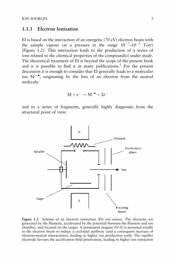
EI is based on the interaction of an energetic (70 eV) electron beam withthe sample vapour (at a pressure in the range 10�7–10�5 Torr)(Figure 1.2). This interaction leads to the production of a series ofions related to the chemical properties of the compound(s) under study.The theoretical treatment of EI is beyond the scope of the present bookand it is possible to find it in many publications.1 For the presentdiscussion it is enough to consider that EI generally leads to a molecularion Mþ ., originating by the loss of an electron from the neutralmolecule:
M þ e� ! Mþ� þ 2e�
and to a series of fragments, generally highly diagnostic from thestructural point of view:
Figure 1.2 Scheme of an electron ionization (EI) ion source. The electrons aregenerated by the filament, accelerated by the potential between the filament and ionchamber, and focused on the target. A permanent magnet (N–S) is mounted axiallyto the electron beam to induce a cycloidal pathway (and a consequent increase ofelectron-neutral interactions), leading to higher ion production yield. The repellerelectrode favours the acceleration field penetration, leading to higher ion extraction
ION SOURCES 3
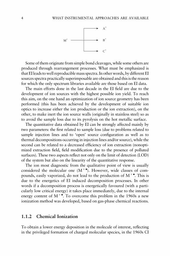
Some of them originate from simple bond cleavages, while some others areproduced through rearrangement processes. What must be emphasized isthat EI leads to well reproduciblemass spectra. In otherwords, by different EIsources spectra practically superimposable are obtained and this is the reasonfor which the only spectrum libraries available are those based on EI data.
The main efforts done in the last decade in the EI field are due to thedevelopment of ion sources with the highest possible ion yield. To reachthis aim, on the one hand an optimization of ion source geometry has beenperformed (this has been achieved by the development of suitable ionoptics to increase either the ion production or the ion extraction), on theother, to make inert the ion source walls (originally in stainless steel) so asto avoid the sample loss due to its pyrolysis on the hot metallic surface.
The quantitative data obtained by EI can be strongly affected mainly bytwo parameters: the first related to sample loss (due to problems related tosample injection lines and to ‘open’ source configuration as well as tothermal decompositions occurring in injection lines and/or source), while thesecond can be related to a decreased efficiency of ion extraction (nonopti-mized extraction field, field modification due to the presence of pollutedsurfaces). These two aspects reflect not only on the limit of detection (LOD)of the system but also on the linearity of the quantitative response.
The ion most diagnostic from the qualitative point of view is usuallyconsidered the molecular one (Mþ .). However, wide classes of com-pounds, easily vaporized, do not lead to the production of Mþ .. This isdue to the energetics of EI induced decomposition processes. In otherwords if a decomposition process is energetically favoured (with a parti-cularly low critical energy) it takes place immediately, due to the internalenergy content of Mþ .. To overcome this problem in the 1960s a newionization method was developed, based on gas-phase chemical reactions.
1.1.2 Chemical Ionization
To obtain a lower energy deposition in the molecule of interest, reflectingin the privileged formation of charged molecular species, in the 1960s CI
A+
B+
C+
M+
4 WHAT INSTRUMENTAL APPROACHES ARE AVAILABLE

methods were proposed.2 They are based on the production in the gasphase of acidic or basic species, which further react with a neutralmolecule of analyte leading to [MþH]þ or [M � H]� ions, respectively.Generally, protonation reactions of the analyte are those more widelyemployed; the occurrence of such reactions is related to the proton affinity(PA) of M and the reactant gas, and the internal energy of the obtainedspecies are related to the difference between these proton affinities. Thus,as an example, considering an experiment performed on an organicmolecule with PA value of 180 kcal/mol (PAM), it can be protonated by re-action with CHþ
5 (PACH4¼ 127 kcal/mol), H3Oþ (PAH2O ¼ 165 kcal/mol),
but not with NHþ4 (PANH3
¼ 205 kcal/mol).3 This example shows animportant point about CI: it can be effectively employed to select speciesof interest in complex matrices. In other words, by a suitable selection of areacting ion [AH]þ one could produce [MH]þ species of molecules withPA higher than that of A. Furthermore the extension of fragmentation canbe modified in terms of the difference of [PAM – PAA].
From the operative point of view CI is simply obtained by introducingthe neutral reactant species inside an EI ion source in a ‘close’ configura-tion, by which quite high reactant pressure can be obtained (Figure 1.3).
Figure 1.3 Scheme of a chemical ionization (CI) ion source. The electron entranceand ion exit holes are of reduced dimension in order to obtain, inside the ionchamber, effective pressure of the reagent gas
ION SOURCES 5

If the operative conditions are properly set the formation of abundant[AH]þ species (or, in the case of negative ions B�) is observed in highyield. Of course, attention must be paid in particular in the case ofquantitative analysis to reproduce carefully these experimental condi-tions, because they reflect substantially on the LOD values.
CI, as well as EI, requires the presence of samples in vapour phase andconsequently it cannot be applied for nonvolatile analytes. Efforts havebeen made from the 1960s to develop ionization methods overcomingthese aspects and, among them, field desorption (FD)4 and fast atombombardment (FAB)5 resulted in highly effective methods and opened newapplications for mass spectrometry. More recently new techniques havebecome available and are currently employed for nonvolatile samples:APCI,6 ESI,7 APPI8 and MALDI9 represent nowadays the most used forthe analysis of high molecular weight, high polarity samples.
For these reasons, we describe these methods.
1.1.3 Atmospheric Pressure Chemical Ionization
APCI6 was developed starting from the consideration that the yield of agas-phase reaction does not depend only on the partial pressure of thetwo reactants, but also on the total pressure of the reaction environ-ment. For this reason the passage from the operative pressure of0.1–1 Torr, present inside a classical CI source, to atmospheric pressurewould, in principle, lead to a relevant increase in ion production and,consequently, to a relevant sensitivity increase.
At the beginning of the research devoted to the development ofthe APCI method, the problem was the choice of the ionizing device.The most suitable and effective one was, and still is, a coronadischarge. The important role of this ionization method mainly liesin its possible application to the analysis of compounds of interestdissolved in suitable solvents: the solution is injected in a heatedcapillary (typical temperatures in the range 350–400 �C), whichbehaves as a vaporizer. The solution is vaporized and reaches outsidefrom the capillary the atmospheric pressure region where the coronadischarge takes place. Usually the vaporization is assisted by a nitrogenflow coaxial to the capillary (Figure 1.4). The ionization mechanism istypically the same present in CI experiments (Figure 1.5). The solventmolecules, present in high abundance, are statistically privileged tointeract with the electron beam originated from the corona discharge;the ions so formed react with other solvent molecules leading to
6 WHAT INSTRUMENTAL APPROACHES ARE AVAILABLE
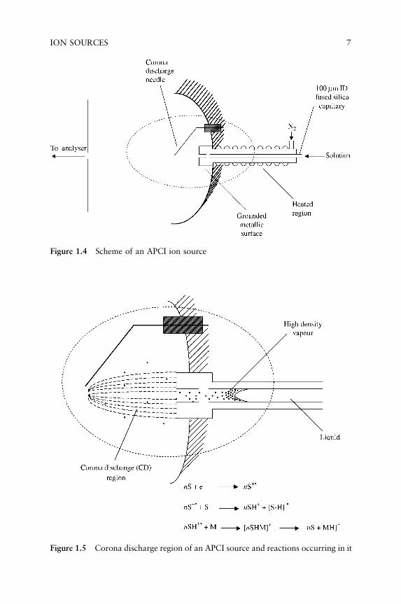
Figure 1.4 Scheme of an APCI ion source
Figure 1.5 Corona discharge region of an APCI source and reactions occurring in it
ION SOURCES 7

protonated (in the case of positive ions analysis) or deprotonated(negative ions analysis) species, which are the reactant for the analyteionization. One problem which, at the beginning of its development,APCI exhibited was the presence of analyte molecules still solvated,i.e. the presence of clusters of analyte molecules with different num-bers of solvent molecules. To obtain a declustering of these species,different approaches have been proposed, among which nonreactivecollision with target gases (usually nitrogen) and thermal treatmentsare those considered most effective and currently employed. Differentinstrumental configurations, based on a different angle between thevaporizer and entrance capillary (or skimmer) have been proposed;180 � (in line) and 90 � (orthogonal) geometries are those most widelyemployed.
In particular, in the case of quantitative analysis, a particular caremust be devoted to finding the best operating conditions (vaporizingtemperature and solution flow) of the APCI source, which lead to themost stable signals, and carefully maintaining these conditions for all themeasurements.
1.1.4 Electrospray Ionization
ESI7 is obtained by injection, through a metal capillary line, of solutionsof analyte in the presence of a strong electrical field. The production ofions by ESI can be considered as due to three main steps: (i) productionof charged drops in the region close to the metal capillary exit; (ii) fastdecreasing of the charged drop dimensions due to solvent evaporationand, through phenomena of coulombic repulsion, formation of chargeddrop of reduced dimension; (iii) production of ions in the gas phaseoriginated from small charged droplets.
The experimental device for an ESI experiment is shown in Figure 1.6.The analyte solution exits from the metal capillary (external diameter,rc, in the order of 10�4 m) to which a potential (Vc) of 2–5 kV is applied;the counter electrode is placed at a distance (d) ranging from 1 to 3 cm.This counter electrode in an ESI source is usually a skimmer with a 10 morifice or an ‘entrance heated capillary’ (internal diameter 100–500 m;length 5–10 cm), which represents the interface to the mass spectro-metric analyser. Considering the thickness of the metal capillary, theelectrical field (Ec) close to it is particularly high. For example, forVc¼ 2000 V, rc¼10�4 m and d ¼ 0:02 m, an Ec in the order of6 � 106 V/cm has been calculated by Pfeifer and Hendricks.10 This
8 WHAT INSTRUMENTAL APPROACHES ARE AVAILABLE

electrical field interacts with solution and the charged species presentinside the solution move in the field direction, leading to the formationof the so called ‘Taylor cone’.11 If the electrical field is high enough, aspray is formed from the cone apex, consisting of small chargeddroplets. In the case of positive ion analysis, i.e. when the needle isplaced at a positive voltage, the droplets bear positive charge andvice versa in the case of negative ion analysis. A charged drop movesthrough the atmosphere for the field action in the direction of thecounter electrode. The solvent evaporation leads to the reduction ofthe drop dimensions and to a consequent increase of the electrical fieldperpendicular to the droplet surface. For a specific value of dropletradius the ion repulsion becomes stronger than surface tension and inthese conditions the droplet explosion takes place.
Two mechanisms have been proposed for the formation of gaseousions from small charged droplets. The first model, called ‘charge residuemechanism’ (CRM) was proposed by Dole in 196812 and describes theprocess as sequential scissions leading to the production of smalldroplets bearing one or more charges but only one analyte molecule.When the last, few solvent molecules evaporate the charge(s) remains
Figure 1.6 Scheme of ESI ion source and enlarged view of droplet generationregion. (Taylor cone and droplet dimension are not to the same scale)
ION SOURCES 9

deposited on the analyte structure, which gives rise to the most stablegaseous ion.
More recently, Iribarne and Thomson have proposed a differentmechanism, describing the direct emission of gaseous ions from thedroplets, after it has reached a certain dimension.13 This process, calledthe ‘ion evaporation mechanism’ (IEM) is predominant on the coulom-bic fission for droplets of radius, r, lower than 10 m.
From the above, the reader can consider the factors which can affectthe ion production and consequently the sensitivity and reproducibilityin ESI measurements. The ion intensity exhibits with respect to analyteconcentration a typical trend, analogous to that reported, as an exam-ple, in Figure 1.7. A linear portion with a slope of about 1 is present forlow concentration until 10�6 M, followed by a slow saturation with aweak intensity decreasing at the highest concentrations (10�3 M). Thelinear portion, where intensity is proportional to concentration, is theonly region suitable for quantitative analysis. The general trend of theplot can be explained considering that in the system there is not just asingle analyte: further electrolytes are always present, for example,impurities, co-analytes and buffer. It should be emphasized that foranalyte concentrations lower than 10�5 M, the electrospray phenom-enon occur due to the presence of electrolytes as impurities, which leadto the electrical conductivity necessary for the ‘Taylor cone’ production.
Also, in the case of ESI sources, ‘in line’ or ‘orthogonal’ geometrieshave been proposed and employed.
Figure 1.7 Plot of ion intensity vs analyte (morphine HCl) concentration obtainedby ESI experiments. Reprinted from P. Kebarle and L. Tang, Anal. Chem. 65, 980A(1993), with permission from the American Chemical Society
10 WHAT INSTRUMENTAL APPROACHES ARE AVAILABLE

1.1.5 Atmospheric Pressure Photoionization
A method recently developed consists in the irradiation, by a normalkrypton (Kr) lamp, of the vaporized solution of the sample of interest atatmospheric pressure (APPI).8 The instrumental set up is very similar tothat already described for the APCI system (Figure 1.8). In this case, theneedle for corona discharge is no longer present, while the solutionvaporizer is exactly the same as for the APCI source. On a side of thesource the Kr lamp is mounted, so that the vapour solution can beirradiated by photons with energies up to 10.6 eV. The photoionizationfollows a simple general rule: a molecule with ionization energy (IEM)can be ionized by photons with energy En¼hn only when:
IEM � En
Considering that the most of solvents employed in liquid chromato-graphy (LC) methods have an IE higher than 10.6 eV and consequentlycannot be ionized by interaction with photon coming from the Kr lamp,the APPI method seems to be, in principle, highly effective for liquidchromatography/mass spectrometry (LC/MS) analysis of compounds
Figure 1.8 Scheme of an APPI ion source
ION SOURCES 11

exhibiting IE lower than 10.6 eV. In the case of compounds of interestwith IE > 10.6 eV, the use of dopants (i.e. substances photoionizableacting as intermediates in the ionization of the molecule of interest) hasbeen proposed.8
Some investigations have shown that some unexpected reactions cantake place in the APPI source, indicating that it can be applied not onlyfor analytical purposes but also for fundamental studies of organic andenvironmental chemistry.14
1.1.6 Matrix-assisted Laser Desorption/Ionisation
MALDI9 consists of the interaction of a laser beam with a solid sampleconstituted by a suitable matrix in which the analyte is present at verylow molar ratio (1:10 000) (Figure 1.9). This interaction leads to the
Figure 1.9 Scheme of MALDI ion source and reactions occurring in the highdensity plume originated by laser irradiation. BS, beam splitter (a portion of the laserbeam is used to start the spectrum acquisition); A, attenuator (to regulate the laserbeam intensity); L, focusing lens, S, slit; M, mirror
12 WHAT INSTRUMENTAL APPROACHES ARE AVAILABLE
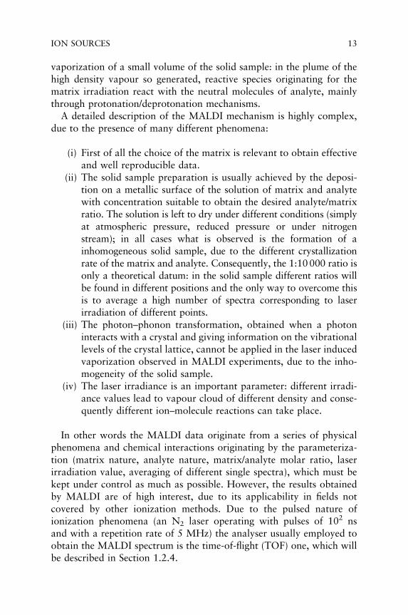
vaporization of a small volume of the solid sample: in the plume of thehigh density vapour so generated, reactive species originating for thematrix irradiation react with the neutral molecules of analyte, mainlythrough protonation/deprotonation mechanisms.
A detailed description of the MALDI mechanism is highly complex,due to the presence of many different phenomena:
(i) First of all the choice of the matrix is relevant to obtain effectiveand well reproducible data.
(ii) The solid sample preparation is usually achieved by the deposi-tion on a metallic surface of the solution of matrix and analytewith concentration suitable to obtain the desired analyte/matrixratio. The solution is left to dry under different conditions (simplyat atmospheric pressure, reduced pressure or under nitrogenstream); in all cases what is observed is the formation of ainhomogeneous solid sample, due to the different crystallizationrate of the matrix and analyte. Consequently, the 1:10 000 ratio isonly a theoretical datum: in the solid sample different ratios willbe found in different positions and the only way to overcome thisis to average a high number of spectra corresponding to laserirradiation of different points.
(iii) The photon–phonon transformation, obtained when a photoninteracts with a crystal and giving information on the vibrationallevels of the crystal lattice, cannot be applied in the laser inducedvaporization observed in MALDI experiments, due to the inho-mogeneity of the solid sample.
(iv) The laser irradiance is an important parameter: different irradi-ance values lead to vapour cloud of different density and conse-quently different ion–molecule reactions can take place.
In other words the MALDI data originate from a series of physicalphenomena and chemical interactions originating by the parameteriza-tion (matrix nature, analyte nature, matrix/analyte molar ratio, laserirradiation value, averaging of different single spectra), which must bekept under control as much as possible. However, the results obtainedby MALDI are of high interest, due to its applicability in fields notcovered by other ionization methods. Due to the pulsed nature ofionization phenomena (an N2 laser operating with pulses of 102 nsand with a repetition rate of 5 MHz) the analyser usually employed toobtain the MALDI spectrum is the time-of-flight (TOF) one, which willbe described in Section 1.2.4.
ION SOURCES 13

1.2 MASS ANALYSERS
The mass analysis of ions in the gas phase is based on their interactionwith electrical and magnetic fields. Originally the main component ofthese devices was a magnetic sector which separates the ions withrespect to their m/z ratio. Until the 1960s most of the mass spectro-meters devoted to physics, organic and organometallic chemistry werebased on this approach, and high resolution conditions were (and stillare) generally acquired by the use of an electrostatic sector. The double-focusing instruments were (and are) of large dimension (at least 2 m2)and required the use of heavy magnet and large pumping systems.
In the 1960s, mainly due to the efforts of the Paul group at BonnUniversity, the development of devices based on electrodynamic fieldsfor mass analysis led to the production of quadrupole mass filters andion traps of small dimension, so that the mass spectrometer became abench-top instrument.
The ease of use of these devices, the ease of interfacing them with datasystems and, over all, the relatively low cost were the factors that movedmass spectrometry from high level, academic environments to applica-tion laboratories, in which the instrument is considered just in terms ofits analytical performances.
In this section, the analysers currently most widely employed will bedescribed, in terms of the physical phenomena on which they are based,of their performances and their ease of use.
1.2.1 Mass Resolution
The main characteristic of a mass analyser is its resolution, defined as itscapability to separate two neighbouring ions. The resolution necessaryto separate two ions of mass M and (M þ�M) is defined as:
R ¼ M=�M
Then, as an example, the resolution necessary to separate N2þ (exact
mass¼28.006158) from COþ (exact mass¼ 27.994915) is:
R ¼ M=�M ¼ 28=0:011241 ¼ 2490
From the theoretical point of view, the resolution parameters can bedescribed by Figure 1.10. It follows that a relevant parameter is the
14 WHAT INSTRUMENTAL APPROACHES ARE AVAILABLE

valley existing between the two peaks. Usually resolution data arerelated to 10 % valley definition.
If the peak shape is approximately gaussian the resolution can be obtainedby a single peak. In fact, as shown by Figure 1.10, the mass difference, �M,is equal to the peak width at 5 % of its height and, accordingly to thegaussian definition, it is about two times the full width at half maximumheight (FWHM). Consequently, by this approach it is possible to estimatethe resolution of a mass analyser simply by looking at a single peak, withoutintroduction of two isobaric species of different accurate mass.
The resolution present in different mass analysers can be affected bydifferent parameters and different definitions can be employed. Thus, inthe case of a magnetic sector instrument the above 10 % valley definitionis usually employed, while in the case of a quadrupole mass filter theoperating conditions are such to keep �M constant through the entiremass range. Consequently, in the case of a quadrupole mass filter theresolution will be 1000 at m/z 1000 and 100 at m/z 100, while in thecase of magnetic sector the resolution will be, for example, 1000 at m/z1000 and 10 000 at m/z 100.
This parameter will be useful to evaluate and compare the perfor-mances of different instrumental approaches.
1.2.2 Sector Analysers
At the beginning of the last century, after fundamental studies byThompson and Aston, which led to the development of the first effective
Figure 1.10 Mass resolution parameters
MASS ANALYSERS 15

mass spectrograph, the first sector instrument was developed by Demp-ster.15 As shown in Figure 1.11, in the Dempster instrument the ions areaccelerated by means of a negative potential which could be changedfrom 500 to 1750 V. The ion beam collimated by the slit S1 enters inuniform magnetic field B.
From the equations:
mv2=2 ¼ zVðkinetic energy ¼ potential energyÞ ð1:1Þ
and
mv2=R ¼ zvBðcentrifugal force ¼ centripetal forceÞ ð1:2Þ
it follows that:
m=z ¼ B2R2=2V ð1:3Þ
where m is ion mass, z is ion charge, V is acceleration potential, v isspeed acquired by the ion after acceleration and R is the circularpathway radius of the ion inside the magnetic field.
Pumps
IS
S1S2
D
B•
Figure 1.11 Dempster mass spectrometer. IS, ion source; S1, ion source slit; B,180 � magnetic field; S2, collector slit; D, electrostatic detector
16 WHAT INSTRUMENTAL APPROACHES ARE AVAILABLE

This shows the capability of a magnetic analyser to separate ions withdifferent m/z ratios with respect to B or V. By scanning B or V it is thenpossible to focus, through the slit S2, all the ionic species generatedinside the source, separated and ordered with respect to their m/z ratio.Dempster chose to perform the acceleration voltage scan, being difficultat that time to perform regular and reproducible B scans. Dempstercalled his instrument a ‘mass spectrometer’ but this definition wasdebated by Aston.16 In fact, using R from Equation (1.2) one can obtain:
R ¼ mv=Bz ð1:4Þ
This relationship shows that all the ions entering the magnetic fieldand having the same charge and the same momentum, follow a circularpathway with an equal radius R, independently from their mass, whileions with different momenta follow pathways of different radii. For thisreason, Aston suggested that the most appropriate term for Dempster’sinstrument would be ‘momentum spectrometer’ and not ‘mass spectro-meter’. However, for ions generated inside the ion source, Equation(1.3) is valid and the term ‘mass spectrometer’ is appropriate.
The physical application of mass spectrometers for the determinationof natural isotope ratios and accurate mass of different nuclides gave riseto the development of instruments with high performance, in particularwith increasing resolution. This led to the design of instruments basedon the use of magnetic and electrostatic sectors.17 The researchersengaged in these developments determined that the resolution is mainlyaffected by four different factors:
(i) ion beam spatial divergence;(ii) kinetic energy distribution of ions with the same m/z value;(iii) the curvature radius of the ion pathway inside the magnetic field;(iv) the width of the ion source and collector slit.
The ion beam emerging from an ion source is, in general, inhomoge-neous either in direction or in kinetic energy. It means that the ion beamis partially divergent and consequently it enters in the analyser regionwith directions inside a y angle. With respect to kinetic energy distribu-tion, it must be taken into account that not all ions generated insidethe ion source experiment the same accelerating field, the potentialbeing inhomogeneous inside the source itself and, considering thatmv2=2 ¼ zV, the V inhomogeneity is reflected in the kinetic energyinhomogeneity.
MASS ANALYSERS 17

Both these negative aspects are corrected by the use of magnetic andelectrostatic sectors.
In 1933 Stephens18 demonstrated that a magnetic sector leads todirection focusing of the ion beam. Just from the descriptive point ofview let us consider the trajectory of an ion beam generated by thesource S and focused by the magnetic field at the point C (Figure 1.12).The beam pathway is perpendicular to the field and follows the curveof radius r. If an ion enters the magnetic sector with an angle lowerthan 90 �, it undergoes the field action for a longer time and conse-quently its deviation will be wider, leading to its focusing at C. If theangle is greater than 90 � the residence time inside the magnetic fieldwill be lower: its deviation will be smaller and the ion will again befocused at C. From the qualitative point of view, we can say that amagnetic sector focuses at the same point all ions having the samemass, charge and velocity. Hence, a magnetic sector exhibits not only aseparating power, but also a focusing one. For these reasons, instru-ments employing a magnetic sector as a mass analyser were commonlycalled ‘single focusing instruments’, leading to direction focusing of theion beam.
The use of electrostatic sectors is highly effective to overcome theinhomogeneity in kinetic energy. In these devices the ions are subjectedto the action of a radial electrostatic field E with direction perpendicularto B. In the field E, generated by two parallel electrodes of cylindricalsection (Figure 1.13), the ions are subjected to the action of a centripetalforce zE. Calling mv2=R their centrifugal force it will be:
zE ¼ mv2=R ð1:5Þ
Figure 1.12 Direction focusing action of a magnetic sector
18 WHAT INSTRUMENTAL APPROACHES ARE AVAILABLE

which, considering that zV ¼ 12 mv2, leads to the equation:
R ¼ 2V=E ð1:6Þ
This equation shows that ions accelerated by V and subjected to theaction of E follow a circular pathway of radius R, independently fromtheir mass. For E¼ constant, only the ions with identical kinetic energypass through the exit slit: the electrostatic sector consequently acts as akinetic energy filter. Hence analysers employing B and E fields (forexample, Figure 1.14) are called ‘double focusing instruments’.19
Double-focusing instruments exhibit a resolution up to 100 000. Ofcourse the maximum value of resolution corresponds to very narrow slitwidth and consequently can be achieved in low sensitivity conditions.
1.2.3 Quadrupole Analysers
Quadrupole mass filter20,21 and quadrupole ion trap22,23 are currentlythe mass analysers most widely employed. They were both developed bythe Paul group (Nobel Prize for physics in 1989) at Bonn University. Thetheoretical data of the behaviour of an ion in a quadrupole electricalfield is highly complex. Here only a picture of such behaviour is given inorder to give the reader a view of what is happening inside these devices.
Both systems start from the same considerations: ions of different m/zvalues will interact in a different manner with alternate electrical fields
Figure 1.13 Velocity focusing action of an electrostatic sector
MASS ANALYSERS 19

Fig
ure
1.1
4Sch
eme
of
adouble
focu
sing
mass
spec
trom
eter
.L
1,
firs
tfiel
d-f
ree
regio
n;
L2,
seco
nd
fiel
d-f
ree
regio
n

(radio frequency, RF). Many different devices were developed to studythis interaction21 but, in the analytical world, the quadrupole mass filterand ion trap are the most widely employed.
1.2.3.1 Quadrupole Mass Filter20,21
Let us consider an ion ejected from an ion source interacting with aquadrupole field generated by four hyperbolic section rods, as shown inFigure 1.15. On the rods a potential of the type U � Vcos ot is applied(where U is the direct current potential and Vcos ot is the RF potential).Ions which enter in this system oscillate in both x and y directions by theaction of this field.
Let us consider the parameters that affect this motion; they are the ionm/z value, the U, V, o values and r0, i.e. the dimension of the mass filter.If we define now two quantities taking into consideration all theseparameters, i.e.:
a ¼ 4zU=mr 20 o
2 ð1:7Þ
q ¼ 2zV=mr 20 o
2 ð1:8Þ
it is possible to draw a ‘stability diagram’ of the device, i.e. to define thea and q values by which the ions follow ‘stable’ trajectories inside the
Figure 1.15 Quadrupole mass filter. The ions are injected in the z direction
MASS ANALYSERS 21

inter-rod space. Outside this stability diagram the a and q values will besuch that the ions will discharge on the rods. The stability diagramusually employed for a quadrupole mass filter is reported in Figure 1.16.
Looking at the a and q definitions it follows that ions with different m/zvalues exhibit different values of a and q. Furthermore, keeping U, V and oconstant, it is possible to overlap on the same diagram a straight line, whoseslope is dependent on the a/q ratio. In fact, the a/q ratio can be calculated as:
a=q ¼ ð4zU=mr20o
2Þðmr20o
2=2zVÞ ¼ 2U=V ð1:9Þ
which leads to
a ¼ ð2U=VÞq ð1:10Þ
This equation represents a straight line in the a, q space, crossing theorigin of axes and whose slope is dependent on the U/V ratio. If wechoose suitable values, a straight line as that reported in Figure 1.16 canbe obtained. It just crosses the apex of the stability diagram and, in theseconditions, all the ions exhibiting a and q values out from the apex willfollow unstable trajectories. If the V and U values are increased, keepingthe U/V ratio constant, ions will increase their a, q values (see Equations1.7 and 1.8) and, when the straight line portion inside the apex of thestability diagram is reached, they will follow stable trajectories, passingthrough the rods and reaching the detector placed after the rodsthemselves. Hence, by scanning both U and V (maintaining the ratioU/V¼ constant) all the ions can be selectively detected.
The above described behaviour well explains the term ‘quadrupolemass filter’ of the device. One point to be emphasized is that by varying
Figure 1.16 q, a stability diagram of a quadrupole mass filter
22 WHAT INSTRUMENTAL APPROACHES ARE AVAILABLE

the U/V ratio it is possible to vary the straight line slope and conse-quently its portion inside the stability diagram. Using this approach it ispossible to play on the peak width/ion current ratio. In other words,moving the straight line closer to the apex it is possible to obtain a betterresolution but the sensitivity may show a significant decrease.
1.2.3.2 Quadrupole Ion Trap22,23
The Paul ion trap is constituted by three electrodes arranged in acylindrical symmetry (Figure 1.17). When a suitable U þ V cosotpotential is applied on the intermediate electrode (ring electrode) andthe two end-cap electrodes are grounded, a quadrupolar field isgenerated and the ions inside the trap follow trajectories confined ina well defined space region. Even in this case the behaviour of the iontrap can be described by defining a and q quantities analogous to thosegiven for the quadrupole mass filter, leading to a stability diagram(Figure 1.18).
Most ion traps commercially available use, as potential applied to thering electrode, only a RF voltage (Vcosot). Consequently the stability
End-cap electrode
End-cap electrode
Ring electrodez0
r0
Figure 1.17 Quadrupole ion trap
MASS ANALYSERS 23

diagram related to the a, q pairs is in this case just a ‘stability line’related to the q values only:
q ¼ �4zV=mr20o
2 ð1:11Þ
From this equation it follows that, for constant values of V, r0 and o,ions of different m/z values exhibit different q values and one canimagine different ions lying on the q axis at q values inversely propor-tional to their m/z values (Figure 1.19). If m/z, V, ro and o values areappropriate, all the ions remain trapped inside the device. By scanning
Figure 1.18 q, a stability diagram of a quadrupole ion trap
Figure 1.19 Portion of the stability diagram of a quadrupole ion trap. In the absenceof U (DC) component, decreasing q values correspond to ions of increasing m/z values
24 WHAT INSTRUMENTAL APPROACHES ARE AVAILABLE

V, the q values of the various ions increase and once their q valuereaches the limit of the stability diagram their trajectory increases alongthe z axis: they are ejected from the trap and detected.
It is to be emphasized that the quadrupole ion trap has specificbehaviour that makes it unique. First of all MS/MS experiments (whichwill be discussed in detail in Section 1.5.3) are easy to perform and thefragmentation yield is so high that sequential collisional experiments(MSn) can be performed.23 Secondly, the resolution available by ion traphas been proven to be up to 106.23 Unfortunately, instruments with theselatter performances are not still available and only resolution of a fewthousand are present in commercial instruments, employed only forpartial portions of the mass spectrum. Furthermore two other pointsare worth noting: on the one hand, the theoretical high mass rangeavailable, obtained by the use of a supplementary RF voltage (ion trapwith mass range up to m/z 8000 are available); on the other, the highsensitivity of the device (ions produced are not lost during the scanning).23
These facilities have led to the production of an ion trap with powerfulperformances for gas chromatography/mass spectrometry (GC/MS) andLC/ESI(APCI)/MS systems.
1.2.4 Time-of-flight
Time-of-flight (TOF)24 is surely, from the theoretical point of view, thesimplest mass analyser. In its ‘linear’ configuration it consists only of anion source and a detector, between which a region under vacuum, withoutany field, is present. Ions with a m/z accelerated by the action of a field Vacquire a speed v. The potential energy will be equal to the acquiredkinetic energy (Equation 1.1). If, from this equation, we put in the v value:
v ¼ ½ð2zV=mÞ 1=2 ð1:12Þ
it is easy to observe that ions of different m/z values exhibit differentspeeds, inversely proportional to the square root of their m/z values. Ifthe ion follows a linear pathway inside a field-free region of length l,considering that v¼ l/t, i.e. t¼ l/v, it follows that:
t ¼ lðm=2zVÞ1=2 ð1:13Þ
This equation shows that ions of different m/z value reach the detectorat different times, proportional to the square root of their m/z value. Forthis reason this device is called ‘time-of-flight’ (Figure 1.20).
MASS ANALYSERS 25

The calibration of the time scale with respect to m/z value can beeasily obtained by injection of samples of known mass.
Of course, this analyser cannot operate in a continuous mode as thesector and quadrupole ones. In this case, an ion pulsing phase isrequired: the shorter the pulse, the better defined is the mass valueand the peak shape.
Furthermore, the ions emerging from the source are usually nothomogenous with respect to their speed (this effect mainly arises fromthe inhomogeneity of the acceleration field). Of course, a distribution ofkinetic energy will reflect immediately on the peak shape and widekinetic energy distribution will lead to enlarged peak shape, with theconsequent decrease in resolution. To overcome this, differentapproaches have been proposed and that usually employed consists ofa reflectron device. As shown in Figure 1.21, the reflectron is constitutedby a series of ring electrodes and a final plate. The plate is placed at afew hundred volts over the V values employed for ion acceleration. Byusing a series of resistors, the different ring electrodes are placed atdecreasing potentials. When an ion beam with kinetic energy Ek ��Ek
interacts with this field, the ion with excess kinetic energy (Ek þ�Ek)
Figure 1.20 Scheme of a linear TOF mass analyser
Figure 1.21 Scheme of reflectron TOF
26 WHAT INSTRUMENTAL APPROACHES ARE AVAILABLE

will penetrate that field following a pathway longer than that followedby ions with mean kinetic energy Ek. In contrast, ions with lower kineticenergy will follow a shorter pathway. This phenomenon leads to athickening of the ion arrival time distribution with a consequent,significant increase in mass resolution.
Nowadays, TOF systems with resolution up to 20 000 are commer-cially available.
1.3 GC/MS25
The coupling of a mass spectrometer with a gas chromatographic systemwas realized in the 1960s and immediately the scientific communityrecognized the high power of the system. In the beginning the onlychromatographic columns available were packed ones, operating withcarrier gas flows in the order of 10 mL/min. Considering the simplerelationship between pumping speed (P, L/s) and gas flow (f, mL/min)corresponding to the maintenance of a vacuum in the order of 10�5
Torr:
P ¼ 103f ð1:14Þ
It follows that a direct coupling of a packed column with a massspectrometer is practically impossible and consequently the use of aHe separator was necessary. This led, at the beginning of GC/MSdevelopment, to severe limitations of the system, which completelydisappeared when capillary columns were introduced. Nowadays, GC/MS systems are robust, reliable, sensitive and highly specific instru-ments. Their main power is due to the fact that they can be effectivelyemployed for qualitative and quantitative analyses. In most systems, thechromatographic column directly reaches the ion source, usually oper-ating in EI and CI conditions.
The system can operate in three different modes, briefly describedbelow.
1.3.1 Total Ion Current (TIC) Chromatogram
The chromatogram is obtained by sequential MS scanning (typical times arein the order 0.2–0.5 s); the data system takes the sum of the signal due todifferent ions present in each spectrum (TIC) and plots the signal so
GC/MS25 27
obtained with respect to the analysis time. The chromatograms are conse-quently related to the TIC due to the background (baseline) and to thedifferent components eluting from the chromatographic column (chroma-tographic peaks).
For quantitative analysis it must be taken into consideration thatdifferent compounds exhibit a different ionization yield and conse-quently lead to a different TIC signal. For such a reason, the use of aninternal standard (IS) is essential to obtain reliable quantitative data.These aspects will be discussed in detail in Chapters 2 and 3.
For the qualitative point of view, once the data file corresponding tothe TIC chromatogram is obtained, it is easy to obtain the mass spectraof various components by just looking at the data with respect to theirretention time.
1.3.2 Reconstructed Ion Chromatogram (RIC)
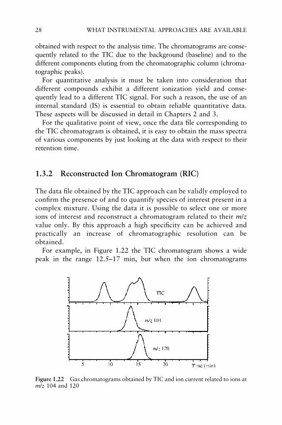
The data file obtained by the TIC approach can be validly employed toconfirm the presence of and to quantify species of interest present in acomplex mixture. Using the data it is possible to select one or moreions of interest and reconstruct a chromatogram related to their m/zvalue only. By this approach a high specificity can be achieved andpractically an increase of chromatographic resolution can beobtained.
For example, in Figure 1.22 the TIC chromatogram shows a widepeak in the range 12.5–17 min, but when the ion chromatograms
Figure 1.22 Gas chromatograms obtained by TIC and ion current related to ions atm/z 104 and 120
28 WHAT INSTRUMENTAL APPROACHES ARE AVAILABLE

relating to m/z 104 and 120 values are reconstructed, it is found that thepeak is due to the partial overlapping of two different components.
1.3.3 Multiple Ion Detection (MID)
In the case of trace analysis, it is useful not to perform the scan of all thespectra, but to consider the different m/z values characteristic of themass spectrum of the compound of interest. Using this approach, ahigher speed monitoring of the chromatographic eluate can be obtainedand valid quantitative data are obtained even for species present at ppblevel. This approach can be applied either on mass units or on accuratemass values, leading to an increase of specificity of the method.
1.4 LC/MS26
In the beginning, the coupling of LC with traditional (EI, CI) sources wasunsuccessful, due to the high solvent level present in LC eluate. Someattempts were made to remove the solvent by ‘moving belt’ systems andto use the solvent itself as reactant for low pressure CI experiments. Thesituation changed with the development of atmospheric pressure ionsources, such as in APCI, ESI and, to a minor extent, APPI.
Nowadays these systems are widely employed and allow the applica-tion of mass spectrometry in fields (especially biological and biomedical)which only a few decades were completely off limits.
A typical arrangement for LC/MS measurements is shown inFigure 1.23. It consists of a LC pump, LC column, APCI or ESI sourceand mass spectrometer. The LC pump system and the LC column mustbe chosen considering the source employed. In fact, due to the differentionization mechanisms, each source has its own optimum eluent flowrate and solvent polarity. The APCI source operates properly with eluentflow rates higher than those employed for ESI and is compatible with a
Figure 1.23 Scheme of the LC/MS coupling
LC/MS26 29

nonpolar mobile phase. Typical eluent flow rates employed with an APCIsource are in the range 4.0–0.5 mL/min: below 0.4 mL/min an unstableanalyte signal can be observed due to nonreproducible discharge pro-cesses. This implies the use of a conventional LC pump and normal(3–4.6 mm ID) and narrow-bore (1–2 mm ID) LC column.
A modern ESI source can work with eluent flow rate up to 1 mL/min,even if the optimum value is about 0.2–0.3 mL/min. A normal LCcolumn can be used by splitting the eluent before the entrance in the ESIsource, while narrow-bore LC columns are normally employed withoutsplitting. The most recent ESI developments lead to micro-ESI and nano-ESI, employed for high sensitivity measurements and applications wheresample amounts are limited (i.e. proteomic, pharmacokinetic studies,etc.). Flow rates in the range 100–10 000 nL/min are normally usedand can be obtained by a capillary LC pump, equipped with a capillary(0.15–0.8 mm ID) and nano (20–100 mm ID) LC column.
As in the case of GC/MS, TIC chromatogram, RIC and MID can beobtained.
1.5 MS/MS27
MS/MS is based on the use of a first mass analyser, employed to selections of interest, and a second mass analyser devoted to the analysis ofthe decomposition products of the preselected ions.
The MS/MS experiment can be subdivided into four different steps:
(i) ion generation;(ii) ion selection;(iii) selected ion decomposition;(iv) mass analysis of the selected ion decomposition products.
These steps can occur in different space regions and in this case theexperiment is called MS/MS ‘in space’, or in the same space region andconsequently they must be time separated. The latter approach is calledMS/MS ‘in time’.
1.5.1 MS/MS by Double Focusing Instruments
The first experiments of MS/MS were generated by the study of thenaturally occurring decomposition of selected ions in the region between
30 WHAT INSTRUMENTAL APPROACHES ARE AVAILABLE

the magnetic and electrostatic sector of a double focusing instrument(see, for example, Figure 1.14).28 The ions of interest, produced in theion source, were selected by fixing the related B value. The decomposi-tion products were analysed by scanning the electrostatic sector. Inorder to increase the yield of ion fragmentation a ‘collision cell’, i.e. asmall box in which a collision gas (typical pressures in the range10�2–10�3 Torr) was inserted in that region, and a fantastic increaseof product ion abundance number and abundance was observed.The method was called collisional-induced decomposition (CID) andin the first years of its application its main use was in the field ofstructural analysis of gaseous ions.
However, in the 1980s some papers appeared, showing the power ofthe method in the analysis of compounds of interest present in complexmixtures. In fact, without the use of any separative method, it ispossible, by direct introduction of a complex mixture and selection ofthe ion characterizing the analyte, to determine its presence and, in somecases, to obtain some quantitative data.
1.5.2 MS/MS by Triple Quadrupoles
The real introduction of the MS/MS system in the analytical worldstarted with the development of triple quadrupole (QQQ) systems,29
shown schematically in Figure 1.24. The ions of interest (Mþ), producedby the suitable ionization method, are selected by Q1, by choosing theappropriate U and V values. The collision gas is injected in Q2, whichoperates in RF only (i.e. it behaves as an ion lens). The ions originatingby collisionally induced decomposition of Mþ are analysed by Q3.
This instrumental arrangement allows a wide series of collisional experi-ments to be performed, among which the most analytically relevant are:
(i) product ion scan: identification of the decomposition product ofa selected ionic species;
Figure 1.24 Scheme of a triple quadrupole (QQQ) system for MS/MS experiments
MS/MS27 31

(ii) parent ion scan: identification of all the ionic species whichproduce the same fragment ion;
(iii) neutral loss scan: identification of all the ionic species whichdecompose through the loss of the same neutral fragment.
The collisional phenomena occurring in a triple quadrupole (as well asin sector machines) lead to the production of an ion population with awide internal energy distribution, due to the statistics of the preselectedion – target gas interactions. Hence, various decomposition channels,exhibiting different critical energies, can be activated and the resultingMS/MS spectrum is, in general, particularly reach of peaks and, conse-quently, of analytical information.
What are the parameters which one can vary in a MS/MS experimentby QQQ? Two parameters are the nature of the target gas (the larger thetarget dimension, the higher the internal energy deposition on thepreselected ion: in other words, Ar is more effective than He) and itspressure (the higher the pressure, the higher the probability of multiplecollisions leading to increased decompositions: of course the pressuremust not exceed the limit compromising the ion transmission!). But,over all, the kinetic energy of colliding ions, which can be varied bysuitable electrostatic lenses placed between Q1 and Q2, plays a funda-mental role in MS/MS experiments.
1.5.3 MS/MS by Ion Traps
More recently, ion trap showed interesting behaviour for MS/MSexperiments.23 It represents an example of MS/MS ‘in time’. In fact,the sequence ion isolation – collision – product ions analysis is per-formed in the same physical space and consequently must be time-separated. A typical sequence is reported in Figure 1.25.
The ions are generated inside the ion trap (or injected in the trap aftertheir outside generation) for a suitable time, chosen in order to optimizethe number of trapped ions (a too high ion density leads to degraded datadue to space-charge effects). The ions inside the trap exhibit motionfrequency depending on their m/z values. The ion selection phase isachieved by the application, on the two end-caps, of a supplementaryRF voltage with all the ion frequencies but the ion of interest one. In theseconditions all the undesidered ions are ejected from the trap and only thatof interest remains trapped. The collision of the preselected ion is againperformed by resonance with the supplementary RF field with a frequency
32 WHAT INSTRUMENTAL APPROACHES ARE AVAILABLE

corresponding to that of ion motion, but with an intensity such to maintainthe ion trajectory inside the trap walls. The ion collides with the He atoms,present in the trap as buffer gas and, once sufficient internal energy isacquired, it decomposes: the product ions so generated remain trapped andby the main RF scan they are ejected from the trap and detected.
It should be emphasized that the collisional data obtained by ion trapare quite different from those achieved by QQQ. In fact in this case theenergy deposition is a step-by-step phenomenon.30 Each time thatthe ion is accelerated by the supplementary RF field up and down insidethe trap, it acquires, through collision with He atoms, a small amountof internal energy. When the internal energy necessary to activate thedecomposition channel(s) at the lowest critical energy is reached, the ionfragments. In other words, while in the case of QQQ the wide internalenergy distribution from collisional experiments leads to the productionof a large set of product ions, in the case of ion trap only a few productions are detected, originating from the decomposition processes atlowest critical energy.
This aspect could be considered negative from the analytical point ofview: in fact a better structural characterization can be achieved by thepresence of a wider product ions set. But it can be easily and effectivelyovercome by the ability of ion trap to perform multiple MS/MSexperiments. In fact the sequence shown in Figure 1.25 can be repeatedby selection, among the collisionally generated product ions, of an ionicspecies of interest, its collision and the detection of its product ions(MS3). This process can be repeated more times (MSn), allowing on theone hand to draw a detailed decomposition pattern related to low energy
Figure 1.25 Sequential pulses of supplementary and main RF voltages employed toperform MS/MS experiments by ion trap
MS/MS27 33

decomposition channels, and on the other to obtain fragment ions of highdiagnostic value from the structural point of view (and hence analyticallyhighly relevant). Hence, by ion trap it is possible to perform MSn
experiments, which cannot be obtained by the QQQ approach.
1.5.4 MS/MS by Q-TOF
Recently a new MS/MS instrument has become available, exhibiting aspecificity higher than that achieved by QQQ or ion trap systems. It isbased on a ‘hybrid’ configuration, employing mass analysers based ondifferent separation principles. The system, usually called Q-TOF isshown schematically in Figure 1.26. The ion of interest, generated inthe source S, is selected by the quadrupole mass filter Q1. Collisions takeplace in Q2 (a quadrupole operating in RF only). The product ions areanalysed by a TOF analyser. Considering the high resolution conditionsavailable by TOF, by this approach the accurate masses of the collision-ally generated product ions (as well as of the precursor) can be easilyobtained, allowing the determination of their elemental composition. Thispossibility leads to a significant increase in the specificity of MS/MS data.
REFERENCES
1. T. D. Mark and G. H. Dunn (Eds) Electron Impact Ionization, Springer–Verlag, Wien
(1985).
Figure 1.26 Scheme of a Q-TOF system. S, ion source; Q1, quadrupole for theselection of ionic species of interest; Q2, collision region (Q2 operates in RF only);IP, ion pusher; R, reflectron; D, detector
34 WHAT INSTRUMENTAL APPROACHES ARE AVAILABLE

2. A. G. Harrison, Chemical Ionization Mass Spectrometry, CRC Press, Boca Raton
(1983).
3. S. G. Lias, J. E. Bartness, J. F. Liebamnn, J. L. Holmes, R. D. Levin and W. G.
Mallard, J. Phys. Chem. Ref. Data, 17 (Suppl. 1) (1988).
4. H. D. Beckey, Principles of Field Ionization and Field DesorptionMass Spectrometry,
Pergamon, London (1975).
5. M. Barber, R. S. Bordoli, G. J. Elliott, R. D. Sedgwick and A. N. Tyler, Anal. Chem.,
54, 645–657A (1982).
6. A. P. Bruins, Mass Spectrom. Rev., 10, 53–77 (1991).
7. (a) M. Yamashita and J. B. Fenn, J. Phys. Chem., 88, 4451–4459 (1988); (b) M.
Yamashita and J. B. Fenn, J. Phys. Chem., 88, 4671–4675 (1988).
8. D. B. Robb, T. R. Covey and A. P. Bruins, Anal. Chem., 72, 3653–3659 (2000).
9. M. Karas, D. Bahar and U. Griessmann, Mass Spectrom. Rev., 10, 335–357 (1991).
10. R. J. Pfeiffer and C. D. Hendricks, AIAA J., 6, 496–502 (1968).
11. G. L. Taylor, Proc. R. Soc. London Ser. A, 280, 383–387 (1964).
12. M. Dole, L. L. Mack, R. L. Hines, R. C. Mobley, L. D. Ferguson and M. B. Alice, J.
Chem. Phys., 49, 2240–2249 (1968).
13. J. V. Iribarne and B. A. Thomson, J. Chem. Phys., 2287–2294 (1976).
14. P. Traldi and E. Marotta in Advances in Mass Spectrometry, Vol. 16, A. E. Ashcroft,
G. Brenton and J. J. Monagan (Eds), Elsevier, Amsterdam (2004), pp. 275–293.
15. A. J. Dempster, J. Phys. Rev., 11, 316–320 (1918).
16. F. W. Aston, Nature, 127, 813–820 (1931).
17. (a) J. H. Beynon in Mass Spectrometry and its Applications to Organic Chemistry,
Elsevier, Amsterdam (1960), pp. 4–27; (b) F. A. White and G. Wood in Mass
Spectrometry Applications in Science and Engineering, John Wiley & Sons, Inc., New
York (1986), pp. 51–66.
18. W. E. Stephens, Phys. Rev., 45, 513–518 (1934).
19. (a) F. A. White, F. M. Rourke and J. M. Sheffield, Appl. Spectr., 12, 46–52 (1958);
(b) T. Wachs, P. F. Bente and F. W. McLafferty, Int. J. Mass Spectrom. Ion Phys., 9,
333–341 (1972); (c) J. H. Beynon, R. G. Cooks and J. W. Amy, Anal. Chem., 45, 1023
(1973); (d) H. Hintenberger and L. A. Konig, Z. Naturforsch. A, 12, 443–452 (1957);
(e) R. P. Morgan, J. H. Beynon, R. H. Bateman and B. N. Green, Int. J. Mass
Spectrom. Ion Phys., 28, 171–191 (1978).
20. (a) W. Paul and H. Steinwedel, Ger. Pat. 944, 900 (1956); US Pat. 2, 939, 952 (1960);
(b) W. Paul and H. Steinwedel, Z. Naturforsch. A, 8, 44 (1953); (c) W. Paul, H. P.
Reinhard and U. von Zahn, Z. Phys., 152, 153 (1958).
21. P. H. Dawson (Ed.) Quadrupole Mass Spectrometry and its Applications, Elsevier,
Amsterdam (1976).
22. R. E. March and R. J. Hughes, Quadrupole Storage Mass Spectrometry, John Wiley
& Sons, Inc., New York (1989).
23. R. E. March and J. F. J. Todd (Eds) Practical Aspects of Ion Trap Mass Spectrometry,
Vols I–III, CRC Press, Boca Raton (1995).
24. (a) W. C. Wiley and I. H. McLaren, Rev. Sci. Instr., 26, 1150–1157 (1955); (b) R. J.
Cotter, Anal. Chem., 64, 1027A–1039A (1992); (c) B. A. Mamyrin, V.I. Karataev,
D. V. Shmikk and V. A. Zagulin, Sov. Phys.– JETP, 37, 45–48 (1973); (d) B. A.
Mamyrin, Int. J. Mass Spectrom. Ion Proc., 131, 1–19 (1994).
25. J. Abian and E. Gelpi in Mass Spectrometry in Biomolecular Sciences, R. Caprioli, A.
Malorni and G. Sindona (Eds), NATO ASI Series, Series C: Mathematical and
REFERENCES 35

Physical Sciences, Vol. 475, Kluwer Academic Publisher, Dordecht (1996),
pp. 437–460.
26. (a) B. E. Erickson, Anal. Chem., 72, 711A–716A (2000); (b) W. M. Niessen,
J. Chromatogr. A, 856, 179–197 (1999).
27. F. W. McLaffery (Ed.) Tandem Mass Spectrometry, John Wiley & Sons, Inc., New
York, (1983).
28. R. G. Cooks, J. H. Beynon, R. M. Caprioli and G. R. Lester, Metastable Ions,
Elseveier, Amsterdam (1973).
29. R. A. Yost and C. G. Enke in Tandem Mass Spectrometry, F. W. McLaffery (Ed.),
John Wiley & Sons, Inc., New York (1983), pp. 175–195.
30. J. Gronova, C. Paradisi, P. Traldi and U. Vettori, Rapid Commun. Mass Spectrom., 4,
306–313 (1990).
36 WHAT INSTRUMENTAL APPROACHES ARE AVAILABLE
2How to Design a Quantitative
Analysis
Chemical analyses are measure procedures and consequently the generalconcepts of metrology can be applied to them. According to metrology,in order to obtain reliable results from a measurement, it must refer tocertified standards. This allows a valid comparison of measurementsperformed in different conditions and at different times. Furthermore,two different measurements are compatible only when the relateduncertainty value is provided.
In the past most attention was focused on the reproducibility ofmeasurements but nowadays the interest is mainly focused on thepossibility of comparing the results obtained by different laboratories.This interest originates from various aspects of globalization, theincrease and liberalization of work trade, the achievement of uniformityof analysis and medical treatment and the growing, common interest inenvironmental problems and planet health.
In this frame, retention of the calibration procedure is essential. It canbe defined as ‘all the operations which allow to establish, under givenconditions, the relationship between the value of a quantity indicated byan instrument or any other measurement system and the correspondingvalue present in a standard sample’. The results of a calibrationprocedure are given sometimes as a calibration constant or a series ofcalibration constants expressed in a calibration diagram. For an instru-mental measurement this diagram represents the response of the instru-ment itself to different values of the quantity under measurement. Thecurve linking the points so obtained is called the calibration curve. An
Quantitative Applications of Mass Spectrometry I. Lavagnini, F. Magno, R. Seraglia and P. Traldi
# 2006 John Wiley & Sons, Ltd

uncertainty band should be added to the calibration curve. All thesepoints will be treated in detail in Chapter 4.
The calibration of an instrument is a very specific operation that musttake place at a very precise moment. After calibration the instrument canbe used; calibration remains constant for some time. Calibration mustbe checked and sometimes adjustment of the instrument or a newcalibration operation become necessary.
As far as chemistry is concerned, the most required measurements arethe different forms of concentration (mass concentration, volume con-centration, molar fraction and so on). Therefore standard differentsubstances at different concentrations are needed. In general the idealstandard is a sample of a pure substance diluted in known proportionsinto a proper matrix.
Very often the analytical method cannot guarantee either a completeseparation or a complete recovery of the substances present in thematerial to be analysed, or the absence of interferences. For that reasonit is necessary to use a reference matrix as similar as possible to thecomposition of the material to be analysed.
In the case of particularly complex matrices (both organic andinorganic) reference material is not prepared mixing its own compo-nents, but starting from a material similar to the one that has to beanalysed (such as sludges or animal tissue, for instance). The determina-tion of the concentration of each different component is done analyti-cally with specific precautions (and often with the help of several anddifferent laboratories).
It is important to highlight the effort made during recent years notonly by the researchers belonging to different scientific fields to fixstandards fitting all branches of science and technology, but also theeffort made by people working in different sectors to adopt a standardterminology and procedures for solving the problems of measurementquality which may be used in different scientific branches such asphysics, chemistry, clinical chemistry and laboratory medicine.
After these general considerations on the metrology approach, we willfocus our attention on the procedures generally adopted in the projectand design of a quantitative analysis.
2.1 GENERAL STRATEGY
The general strategy employed in the design of a quantitative analysis isshown schematically in Figure 2.1. It consists of many different steps,
38 HOW TO DESIGN A QUANTITATIVE ANALYSIS

each of which is relevant to the achievement of valid results. If, after thedevelopment of the procedure, the data obtained are not satisfactory forthe solution of the analytical problem, the whole procedure must restartwith the use of a different analytical method. On the left side of the flowchart one important parameter, the analysis time, is reported; it becomesparticularly important when the number of samples to be analysed ishigh: in this case a high throughput becomes essential.
In general the cost/benefits ratio of the possible different analyticalapproaches must be evaluated: the low ratio value obtained for mass
Choice of theinternal (external)
standard(s)
Calibrationcurve
Analytical problem
Performance characteristics: detection and quantification capabilities,
selectivity, etc.
Choice at the analytical method(s)
Sampling(s)
Analytical sample preparation
Instrumental measurements
Processing and analitical results
Data evaluation in terms of theanalytical problem
NO
YES
Time
Solution ofthe analytical problem
Figure 2.1 Flow chart of the different steps to be followed in the development of aquantitative analysis
GENERAL STRATEGY 39

spectrometric approaches is not related to the low costs, but rather tothe high value of benefits in terms of sensitivity and specificity, as well asto their high throughput.
The analytical methods mainly employed can be subdivided into twobroad classes, the chemical-physical and immunometric ones. Massspectrometry, with all its possible operative configurations, belongs tothe former group.
At this point it may be useful to define a series of quantities which givethe performance characteristics of an analytical procedure:
ApplicabilityThe applicability pertains to the analyte identity, its concentrationrange, and the acceptable uncertainty.
SpecificityThe specificity is the capability of an analytical method to revealonly one analyte in the presence of other components.
SelectivityThe selectivity is the capability of an analytical method in quanti-fying analytes in the presence of interfering species.
PrecisionThe precision is the accordance among independent resultsobtained in the same operating conditions.
AccuracyThe accuracy evaluates the proximity between the true (or theaccepted reference value) and the found value; the inaccuracycomprises the random error and the bias.
TruenessThe trueness is the proximity between the true (or the acceptedreference value) and the mean value of several repeated measure-ments.
RecoveryThe recovery is the estimation, in per cent, of the amount of thespecies recovered in the analytical procedure.
RangeThe range is defined as the difference between the minimum andmaximum response level.
Linear dynamic rangeThis is the concentration interval where the signal changes linearlywith the analytical concentration.
Critical levelThis is the minimum signal which can be distinguished from thebackground with a defined confidence level.
40 HOW TO DESIGN A QUANTITATIVE ANALYSIS

Limit of detectionThis is the lowest quantity or concentration of the analyte whichcan be detectable with a defined confidence level.
Limit of quantificationThis is the lowest quantity or concentration of the analyte whoseresponse is measured with a defined precision.
SensitivityThis is the slope of the calibration curve.
ResistanceThis quantity expresses the capability of the method to give thesame analytical result for the same sample even in presence ofchanges of experimental conditions (e.g. different laboratories,different instrumentation, different days of analysis).
Robustness (or Ruggedness)This quantity expresses the capability of the method to be notstrongly dependent on small changes in operating conditions (e.g.temperature, pH).
2.1.1 Project
The design of a project for a quantitative analysis is generated by aninput related to the kind of analyte(s) of interest, its possible quantityand the substrate in which the analyte(s) is present. These three pointsmust be carefully analysed to make the best choices in terms of analyterecovery and instrumental set-up.
2.1.2 Sampling
The sampling must be done in a manner which warrants no change inthe analyte composition from the qualitative and quantitative points ofviews, and the achievement of statistically significant results.
Two sampling approaches can be employed, strongly dependent onthe substrate in which the analyte is present. The first is based on on-line, in-field measurements with the instrument present on the site ofinterest and the sampling is carried out by a device directly connected tothe instrument. This is the case, for example, of quadrupole gasanalysers: the gaseous substrate (usually air at atmospheric or reducedpressure) is directly injected in an EI source and the gaseous analytepartial pressures are immediately determined by mass analysis.The second approach, the most common one, is based on off-line
GENERAL STRATEGY 41

measurements: in this case the substrate containing the analyte(s) ofinterest is brought to the laboratory, where analyte extraction proce-dures and instrumental measurements are performed. A mixed proce-dure can also be considered, based on the analyte extraction in thefield and its analysis in the laboratory. This is the case in which sampl-ing cartridges or solid phase microextraction (SPME) devices areemployed.
There are some general rules to be followed for a correct sampling:
(i) the sampling must be carried out by trained and qualifiedpersonnel;
(ii) each lot to be analysed must be sampled separately;(iii) the sampling devices must be appropriate and must guarantee
the absence of any contamination;(iv) the incremental samples must be drawn in different points of the
lot or sub-lot;(v) the aggregate sample is obtained by mixing the incremental
samples;(vi) the laboratory samples are obtained from the homogenized
aggregate sample;(vii) the samples must be suitably stored.
A correct labelling of the laboratory sample is fundamental: it wouldcontain sample name, sampling date and place, and lot and any informa-tion useful for the analyst.
2.1.3 Sample Treatment
The analytical sample preparation is a particularly critical point. Itconsists usually in several steps: analyte extraction from matrix, extractpurification and, when necessary, extract concentration, and chemicaltransformation (derivatization) of the analyte in the form more suitablefor the analysis.
An effective development of the sample preparation for the expectedanalyte levels requires specific knowledge of the chemical and physicalproperties of the analyte and of the matrix. The different sampleextraction procedures commonly employed are summarized in Figure 2.2.Their description is beyond the aim of the present work and the readercan find details on the different approaches in scientific and technicalliterature.
42 HOW TO DESIGN A QUANTITATIVE ANALYSIS

2.1.4 Instrumental Analysis
A quantitative analysis based on MS methods is usually carried out byhyphenated techniques, mainly GC/MS and LC/MS. There are somesimilarities and some differences among the problems arising from thetwo approaches and some of these aspects will be discussed in detail inChapter 3. At this stage the same treatment can be used for bothapproaches. In fact, the same methodologies are employed to obtainthe related chromatogram and the quantitative measurements arealways related to the relationship between instrumental response andsample quantity (or concentration).
2.1.4.1 Quantitative Analysis by GC/MS and LC/MS
GC/MS and LC/MS measurements can be performed in differentoperating conditions:
(i) Full scan. Full scan spectra (in the mass range of interest) arecontinuously recorded, with typical scanning speed in the order0.2–1 s. The chromatographic signal is obtained by the sum ofthe MS signals due to all the ions detected in the selected massrange or to selected ions (full scan – selected extraction ion
Matrix
Solid Liquid
Gas phase extraction• Static head space (SHS)• Dynamic head space (DHS)Solid phase microextraction (SPME)Supercritical fluid extraction (SFE)
Solid–liquid extraction• Soxhlet• Ultrasonic extraction• Matrix solid phase dispersion• Accelerated solvent extraction• Microwave assisted extractionSupercritical fluid extraction (SFE)
Liquid–liquid extraction• Separatory funnel• Continuous extraction• Simultaneous distillation extraction (SDE)Solid phase extraction (SPE)Solid phase microextraction (SPME)Stir bar sorptive extraction (SBSE)
Gas phase extraction• Static head space (SHS)• Dynamic head space (DHS)• Purge & trap (P&T)Solid phase microextraction (SPME)Supercritical fluid extraction (SFE)
Volatile
Nonevolatile
Sam
ples
Figure 2.2 Different sample extraction procedures commonly employed
GENERAL STRATEGY 43

profile) when resolution in the m/z domain is utilized to improveinadequate resolution in the time domain. It should be empha-sized that molecules of different structures exhibit differentionization yields and consequently the number of ions (and thechromatographic peak areas) can be different for different com-pounds present in equal molar ratio. For this reason the use of acalibration procedure becomes essential.
(ii) Selected ion monitoring (SIM) or multiple ion detection (MID).The mass spectrometer operates by jumping on m/z values highlydiagnostic for the analyte of interest. By this approach a drasticreduction of the chemical background is obtained; in otherwords, all the components for which the diagnostic ions arenot present in their mass spectra and possibly interfering with theanalyte [with identical or similar retention time (r.t.) values] arenot detected. The SIM (or MID) analysis can be performed byoperating on integer m/z values (i.e. in low resolution conditions)or, as will be described in Chapter 3, on accurate mass values (i.e.in high resolution conditions). Considering that isobaric ions ofdifferent elemental composition lead to different values of accu-rate mass, it follows that by the latter approach a clear increase inspecificity and selectivity is obtained, in their turns reflecting onan increase in detection limits and sensitivity. However, also inthis case, the use of an internal standard is essential.
As an example, the partial TIC chromatogram of a urinesample extract is shown in Figure 2.3(a). The peak at r.t. �19min corresponds to bis-tetramethylsilane derivatives of testoster-one, whose EI mass spectrum is characterized by the presence ofhigh abundant ions at m/z 432 (M+.), 417 ([M – CH3]+) and 301([M – C6H15OSi]+). The absolute quantity of testosterone wasdetermined in the order of 100 pg. The selection and monitoringof the ions at m/z 432, 417 and 301 led to a chromatogram withonly the peak due to testosterone. As shown in Figure 2.3(b), anincrease in detection limits and sensitivity is obtained. Theselected ion signal-to-noise ratio for a sample containing 5 pgis analogous to that shown in Figure 2.3(a) (100 pg).
(iii) MS/MS and MSn. A further increase in specificity and selectivitycan be obtained by collisional experiments on ionic speciesdiagnostic for the analyte and the recording of collisionallyproduced fragment ions. It is easy to achieve the selection of adiagnostic ion, and the production of a diagnostic fragmentpractically eliminates all the interfering species. This method
44 HOW TO DESIGN A QUANTITATIVE ANALYSIS

can be further improved by the use of sequential collision experi-ments (MSn), such as those possible with ion trap instruments.Also, for this approach the use of an internal standard is essential.The recording of the ion current related to collisionally generatedions is usually called selected reaction monitoring (SRM).
2.1.4.2 Calibration Curves
A most rigorous description of this topic is given in Chapter 4. At thispoint, it is useful to give a description on how to obtain a valid calibrationcurve that can be successfully used for quantitative measurements.
Figure 2.3 (a) TIC gas chromatogram of a urine sample containing about 100 pg/mL of testosterone. (b) MID chromatogram of a urine sample containing 5 pg/mL oftestosterone
GENERAL STRATEGY 45

Quantitative measurements are usually based on the construction of arelationship between the instrumental response and the analyte concen-tration/amount. The slope of this curve is called the sensitivity orcalibration factor S. In the case of GC/MS and LC/MS measurementsthe instrumental response is the analyte peak area (as obtained by eitherTIC or selected ion current). This relationship would be, in someconcentration ranges, linear but, due to experimental and/or observa-tional errors, the experimental points are (hopefully weakly) scatteredabout the straight line.
Apart from random fluctuations, the relationship between the instru-mental response and the concentration/amount may be disturbed byinterferences, matrix effects and by the simultaneous presence of thesetwo effects. We here disregard the interference problem as we trust thatthe use of a hyphenated instrument which combines time and m/zresolution can eliminate it. The matrix effect, which modifies thesensitivity of the analysis, must be still considered and can be handledby the addition of standards of the analyte to the sample (StandardAddition Method). However, when the matrix effect is negligible orwhen the matrix can be satisfactorily reproduced, the usual ‘external’calibration procedure can be successfully adopted.
The Standard Addition Method can be used to determine theunknown level of a known analyte in a unreproducible matrix. By thisapproach a plot, as shown in Figure 2.4, is obtained. Once prepared astandard solution of the analyte at known concentration Cst, a constantvolume of the unknown solution Vu is added to each of four (or more)flasks of equal volume Vf. At this point increasing (and well measured)volumes of the standard solution Vst are added to each flask and thesolutions are brought to the same volume by adding solvent and thenmeasured. By this approach it is easy to calculate the unknownconcentration C0 of the analyte. Considering that the analyte concen-tration in a flask can be expressed as:
Cu ¼ ðC0Vu þ CstVstÞ=Vf ¼ C0Vu=Vf þ CstVst=Vf ð2:1Þ
and that the response R is the product of the calibration factor S and theconcentration, Equation (2.1) can be written as:
R ¼ S � C0Vu=Vf þ S � C ð2:2Þ
where C ¼ CstVst=Vf:Equation (2.2) represents a straight line with intercept equal to
S � C0Vu=Vf. The null response is obtained at C ¼ �C0Vu=Vf (Figure 2.5)
46 HOW TO DESIGN A QUANTITATIVE ANALYSIS

Figure 2.4 Peak area calibration with external standard
10
8
6
4
2
00–40 –20
–2
20 40 60 80
Csa, µg/mL
Res
pons
e
x-interceptat y=0
Figure 2.5 Example of the determination of the concentration of a known analyteby standard addition
GENERAL STRATEGY 47
and consequently the unknown concentration C0 can be easily calcu-lated as:
C0 ¼ �CVf=Vu
In other words, by spiking a solution containing the analyte of interest atunknown concentration with known volumes of the analyte standardsolution, it is possible to determine its concentration in the original solution.
2.1.4.3 Internal Standard
In general the analytical procedure is affected by various analyticalerrors, deriving from either sample and standard solutions manipula-tions or instrumental problems (e.g. instability of instrumentalresponse). For these reasons the approach followed implies the additionof an internal standard (IS), which compensates for the various analy-tical errors and is particularly effective in the case of highly complexsubstrates. A known compound at a fixed concentration is added to theunknown sample before any sample treatment and purification proce-dure to give a separate peak in the chromatogram.
It follows that only a high structural similarity between the analyte ofinterest and the IS can guarantee an equal efficiency of extraction of bothfrom the analytical sample and this aspect is fully satisfied when stableisotope labelled derivatives of the analyte are used as the IS. In theseconditions a biunivocal relationship is obtained between the ratio of thepeak areas corresponding to analyte and IS and the molar ratio [analyte]/[IS].
Three kinds of IS are usually employed:
(i) A compound with r.t. value different from that of the analyte,homologous to the analyte, leading to a fragment Aþ identical tothe analyte fragment. In SIM conditions a chromatogram such asthat shown in Figure 2.6(a) is obtained.
(ii) A compound of the same chemical class of the analyte leading toions with the same m/z value [in this case, as in (i), it must exhibit adifferent r.t. value] or a different m/z value (in this case the r.t. valuecan be different or equal to that of the analyte) (see Figure 2.6b).
(iii) A stable isotope labelled derivative of the analyte (usuallycontaining 2H, 13C, 15N or 18O). It will exhibit the same r.t.value as the analyte but different m/z value (Figure 2.6c). Thisrepresents the most valid approach, but it clashes with the cost oflabelled standard compounds.
48 HOW TO DESIGN A QUANTITATIVE ANALYSIS

It must be emphasized that labelled standard must satisfy somerequirements. Thus, in the case of deuterated derivatives:
� at least three deuterium atoms must be present in the molecule, tolead to a mass shift of three units from the molecular species of theanalyte. For a lower number of deuterium atoms, possible inter-ferences with the isotopic peak of the analyte (M+1, natural 13C-containing and Mþ2 natural 18O-containing species) can occur;
� the percentage of deuterium must be as high as possible and thepercentage of undeuterated component must be as low as possible;
� the deuterium atoms must be introduced in well defined positionsof the molecule, without changing the stereochemistry of themolecule itself;
� the deuterium atoms must be inserted in stable positions, without thepossibility of any exchange with hydrogen during storage and use.
As an example, the structure of 2H3-testosterone employed as IS intestosterone quantitative analysis and the SIM chromatogram related totestosterone and 2H3-testosterone are reported in Figure 2.7.
1% ISA
m/z
min
1% IS A
m/z 1m/z 2
min
1% 1% IS
Am/z 1m/z 2
min
1% IS
Am/z 1m/z 2
min
ISA
m/z
min
(a)
(b)
(c)
Figure 2.6 Examples of the different results obtained in SIM conditions by the useof different IS: (a) compound with a r.t. different from the analyte, leading to afragment of the same m/z value of that chosen for the analyte (A) detection; (b)compound of the same chemical class of the analyte giving a ionic species isobaricwith the analyte (left) or with a different m/z value and different (centre) and equal(right) retention; (c) a stable isotope labelled derivative of the analyte. It will exhibitthe same r.t. of the analyte, but a different m/z value
GENERAL STRATEGY 49

Fig
ure
2.7
SIM
chro
mato
gra
mof
test
ost
erone
(m/z
288)
and
2H
3-t
esto
ster
one
(m/z
291)

The calibration curve is obtained by analysis of different samples withdifferent [analyte]/[IS] molar ratio, taking the concentration of IS asconstant. The data obtained for the calibration curve of testosterone,derivatized by hexafluorobutyric acid (HFBA), are reported in Fig-ure 2.8. The calibration curve has been obtained from the partial SIMchromatogram shown in Figure 2.9, from which the peak areas ofanalyte and IS can be easily calculated.
At this stage some comments on the use of stable isotope labelledderivatives as IS are required. Let us consider a theoretical SIM experiment,in which the analyte and the IS with masses different by more than threeunits are injected in quantities A and S, respectively. Consider that theanalyte and the IS give rise to ions at m/z values m1 and m2, respectively.The contributions of the analyte to m1 and m2 intensities are a1A and a2Arespectively, while the contributions of the IS to m1 and m2 are b1S and b2S.In these conditions, the ratio R of the measured peak areas is given by:
R ¼ a1A þ b1S
a2A þ b2Sð2:3Þ
If the isotope labelled IS is isotopically pure, the contribution of theanalyte to mass m2 is negligible, a2A << b2S, and Equation (2.3) becomes:
R ¼ ða1=b2SÞA þ b1=b2 ð2:4Þ
Run
Testosterone (pg/mL)2H3-testosterone (pg/mL)
[Testosterone]/[2H3-testosterone]
1
0
100
0
2
2.5
100
0.025
3
25
100
0.25
4
100
100
1.0
5
250
100
2.5
2.5
1.0
0.250.025
2.5
R
25 100 250 pg/µ L
Are
a m
/z 6
80/A
rea
m/z
683
Figure 2.8 Testosterone, derivatized by HFBA, calibration curve
GENERAL STRATEGY 51

Fig
ure
2.9
SIM
chro
mato
gra
ms
use
dto
ach
ieve
the
cali
bra
tion
curv
ein
Fig
ure
2.8
(HFB
A-t
esto
ster
one
der
ivati
ve:
m/z
680;
2H
3-H
FB
A-
test
ost
erone
der
ivati
ve:
m/z
683)
When the IS is not isotopically pure, b2S becomes smaller, the use of alinear regression straight line as the calibration curve is incorrect and thecalibration function can be only approximated by a quadratic equation.1
2.1.5 Method Validation
At the end of this chapter dealing with the strategy to perform a correctanalysis and with the performance characteristics (see above) whichallow its evaluation, a question arises whether the analytical proceduremeets the intended requirements. The process by which the control isdone is called ‘method validation’. Even if there are different opinionsconcerning the terminology of the performance characteristics, methodvalidation is generally defined as ‘validation of a method establishes, bysystematic laboratory studies, that the method is fit-for-purpose, i.e. itsperformance characteristics are capable of producing results in line withthe needs of the analytical problem’.2
REFERENCES
1. J. R. Chapman and E. Bailey, J. Chromatogr., 89, 215 (1974).
2. CITAC/EURACHEM, Guide to Quality in Analytical Chemistry: An Aid to
Accreditation (2002).
GENERAL STRATEGY 53

3How to Improve Specificity
Of course, any analytical method must be as specific as possible. Thismeans that instrumental data taken into consideration must be strictlyrelated to the physico-chemical properties of the analyte of interest.
In this respect MS is a highly effective technique: for example, in mostcases, the EI spectra well characterize, from a structural point of view,the organic molecule under study on the basis of molecular andfragment ions. This is generally (but not always) true when we considera pure analyte: when it is present, at low concentration, in a complexmixture, its direct identification (and quantification) can be inferred bythe presence of isobaric ions originating from other different compoundspresent in the mixture.
For these reasons the coupling with chromatographic [GC,1 LC,1,2
capillary zone electrophoresis (CZE),3 gel permeation chromatography(GPC),2 supercritical fluid chromatography (SFC)4] methods has been,and is considered, of high interest allowing on the one hand theachievement of mass spectral data of the analyte, possibly without anyinterfering species, and on the other giving further analytical data, i.e.the r.t. values of the different species present in the mixture.
However, even using a chromatographic/MS approach, sometimes theselectivity of the system is not enough to obtain valid and wellreproducible measurements. Consider, for example, an analyte presentat trace level in a matrix so complex to lead to a practically unresolvedchromatogram. In this case the r.t. datum is lost. Furthermore, due tothe very low level of the analyte, both RIC or multiple ion monitoringmeasurements may fail, leading to signals with a very low signal-to-noise ratio, due to the presence of co-eluting species leading to isobaricmolecular or fragment ions.
Quantitative Applications of Mass Spectrometry I. Lavagnini, F. Magno, R. Seraglia and P. Traldi
# 2006 John Wiley & Sons, Ltd

In these cases a higher specificity is required; this chapter is devotedto the possible instrumental approaches which can be employed forthis aim.
3.1 CHOICE OF A SUITABLE CHROMATOGRAPHICPROCEDURE
Of course this choice is strictly related to the physico-chemical proper-ties of the analyte of interest. However, it can be also influenced by twoother aspects:
(i) the instrumental availability in the laboratory;(ii) the ‘cultural’ tradition of the researchers operating in the labora-
tory.
In other words, this choice is affected by the instruments present in thelaboratory and by the knowledge and past experience of the researchers.What is often observed in the literature is that different chromato-graphic/MS approaches are proposed for the same analyte.
In this chapter the methods most widely employed, i.e. GC/MS, andLC/MS, will be described and some examples will be given.
3.1.1 GC/MS Measurements in Low and High ResolutionConditions
A chromatographic process is the result of different phenomena:
� thermodynamic (due to analyte–mobile phase–stationary phaseinteractions)
� kinetic (due to relative motion of the analyte).
A GC system is shown schematically in Figure 3.1. The sample isvaporized into a heated injector (sample introduction in Figure 3.1)and is transferred inside the column by the action of the carrier gas(mobile phase). Separation takes place by the interaction of the variousanalytes with the stationary phase.1
Two different kinds of columns are usually employed for chromato-graphic separation: packed and capillary ones, with internal diameter>0.5 and <0.5 mm, respectively. The former exhibit higher retention
56 HOW TO IMPROVE SPECIFICITY

volume and capacity, while the latter show higher efficiency andpermeability.
Due to its performance, as well as to the lower carrier gas flow,allowing direct coupling with a mass spectrometer, the latter approach isusually employed.
The coupling of GC with MS leads to positive aspects for bothtechniques:
� from the MS point of view, the coupling allows the introductioninside the ion source of the different analytes, (possibly) wellseparated from each other;
� from the GC point of view, MS is a sensitive, universal and specificdetector.
Hence, an increase in specificity is innate in the GC/MS approach, inparticular when the SIM and MID methodologies described in Chapter1 are employed. However, a further, and noteworthy, increase can beobtained when the mass spectrometer is operating at high resolutionconditions. As described in Chapter 1, high resolution allows theaccurate mass value of ions generated from different analytes to bedetermined. The accurate mass is dependent on the elemental composi-tion of the ions. Hence, isobaric ions (i.e. exhibiting the same integermass) of different elemental composition exhibit different values ofexact mass. These different values can be evidenced only by highresolution measurements.
This aspect can be validly employed to increase the selectivity of ameasurement. Consider, as an example, the partial chromatograms
Figure 3.1 Scheme of a gas chromatographic system
CHOICE OF A SUITABLE CHROMATOGRAPHIC PROCEDURE 57

reported in Figure 3.2. The TIC chromatogram (Figure 3.2a) shows, inthe r.t. window of interest, a series of peaks. Consider that we areinterested in the quantification of methyl stearate. Its elemental formula,C19H38O2, leads to an accurate mass value of 298.2872. If we operate inlow resolution conditions, we can perform a SIM experiment selectingthe integer mass value of 298. Using this approach the chromatogram ofFigure 3.2(b) is obtained, which indicates that the peak at r.t. 10.5 mincorresponds to species producing ions (molecular or fragment) at m/z298. At first sight this MID peak could be employed for methyl stearatequantification but, when selectivity is increased by increasing the MSresolution, it follows that only one portion of the chromatographic peakat 10.5 min is due to methyl stearate (Figure 3.2c). The other portion ofthe peak is due to another ionic species with the same integer m/z value(298), but with a different accurate mass value. These two species wereunresolved when operating in low resolution mode and consequentlyquantitative measurements performed in these conditions would lead toincorrect results.
This example does not mean that high resolution conditions arealways essential for the achievement of valid GC/MS results. In mostcases, low resolution MS is more effective and an example of the validityof this approach will be given in the next section. However, in someother cases, in the particular in the presence of highly complex matrices
Figure 3.2 Partial gas chromatogram of a mixture containing methyl stearateobtained in different operating conditions: (a) by TIC; (b) by low resolution multipleion detection of Mþ. of methyl stearate (m/z 298); (c) by high resolution (10 000)multiple ion detection of Mþ. of methyl stearate (m/z 298.2872)
58 HOW TO IMPROVE SPECIFICITY
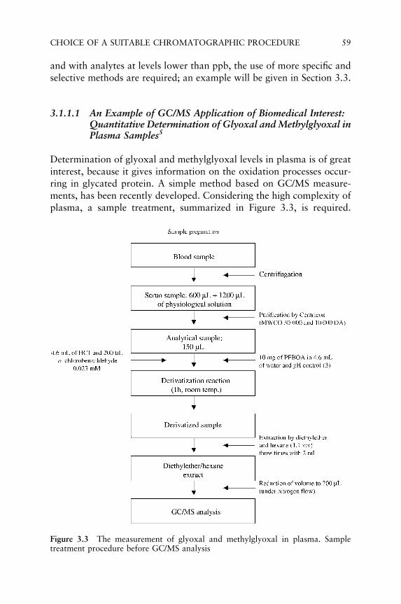
and with analytes at levels lower than ppb, the use of more specific andselective methods are required; an example will be given in Section 3.3.
3.1.1.1 An Example of GC/MS Application of Biomedical Interest:Quantitative Determination of Glyoxal and Methylglyoxal inPlasma Samples5
Determination of glyoxal and methylglyoxal levels in plasma is of greatinterest, because it gives information on the oxidation processes occur-ring in glycated protein. A simple method based on GC/MS measure-ments, has been recently developed. Considering the high complexity ofplasma, a sample treatment, summarized in Figure 3.3, is required.
Figure 3.3 The measurement of glyoxal and methylglyoxal in plasma. Sampletreatment procedure before GC/MS analysis
CHOICE OF A SUITABLE CHROMATOGRAPHIC PROCEDURE 59

Glyoxal and methylglyoxal were evaluated after derivatization withO-(3,3,4,5,6-pentafluorobenzyl)hydroxylamine hydrochloride (PFBOA).The derivatization procedure, described in the literature for glyoxal andmethylglyoxal measurements in various natural matrices6 and partiallymodified for this purpose,5 leads to the formation of O-PFB oximes, asshown in Figure 3.4. To obtain the calibration curve, four solutions ofglyoxal with different concentrations (5.5, 11, 55 and 166 mg/L) wereprepared. In parallel, an IS (o-chlorobenzaldehyde) solution (0.023 mM)was prepared; 150 mL of the various glyoxal solutions and 200 mL of theIS were dissolved in 4.6 mL of an HCl solution (pH 3). After mixing, thepH was carefully checked and adjusted. The resulting solution wastreated with 10 mg of PFBOA and stirred at room temperature for 1 h.After the addition of 0.5 mg of NaCl, O-PFB oximes were extractedwith diethyl ether/hexane 1:1 v/v (3 � 2 mL), stirring for 5 min, and theorganic phase was dried over Na2SO4 and filtered. The volume wasreduced to 0.2 mL under nitrogen flow before GC/MS analysis. Themass spectrometer was operating in low resolution MID modeand signals at m/z 181 (base peak of PFBOA derivatives), 300 (IS)and 448 (the oximes derived from glyoxal) were recorded. The resultingcalibration curve (y ¼ 4:463x þ 16:009) showed a high R2 value(0.9978).
For the analysis of plasma samples, 4.6 mL of HCl solution (pH 3)were added to 150 mL aliquots of the final filtrate. To this solution,200 mL of o-chlorobenzaldehyde solution (0.023 mM) were added andthe pH was adjusted to 3 with a few drops of 0.1 M HCl. Thederivatization procedure was exactly the same as that used for thecalibration curve.
Figure 3.4 Derivatization reaction of glyoxal and methylglyoxal with PFBOAbefore GC/MS analysis. Reproduced from Lapolla et al. (2003)5, with permissionfrom John Wiley & Sons, Ltd
60 HOW TO IMPROVE SPECIFICITY

Methylglyoxal was identified according to literature data: oxime peakrelative r.t. and monitoring the ions at m/z 181 and 462.7,8 Compoundswere quantified on the basis of the sum of signals; concentration ofglyoxal and methylglyoxal were calculated on the calibration line of thesum of glyoxal syn and anti PFBOA dioxime signals. The r.t. of syn andanti o-chlorobenzaldehyde O-PFB oximes and synþ anti and antiþ antimethylglyoxal and glyoxal O-PFB oximes are listed in Table 3.1.
To evaluate the effect of sample storage on glyoxal and methylglyoxalquantitative measurements, plasma samples were stored at �70 �C for 1month: the glyoxal and methyglyoxal levels before and after storageremained practically the same, with variation remaining within theexperimental standard deviation.
An example of the results achievable by this method is shown inFigure 3.5, illustrating the GC/MS results for a healthy subject and adiabetic patient (in the latter case, higher glyoxal and methylglyoxal areto be expected). Peak 1 is due to o-chlorobenzaldehyde, employed as IS,peaks 2 to the stereoisomeric O-PFB oximes of methylglyoxal and peaks3 to the O-PFB oximes of glyoxal. As may be seen from the MIDchromatogram of Figure 3.5, higher abundances of glyoxal and methyl-glyoxal were observed in the plasma sample from the diabetic patient.
The method was applied to the study of glyoxal and methylglyoxallevels for 10 poorly controlled type 2 diabetic patients and a controlgroup of 20 subjects. The obtained results showed that the glyoxal andmethylglyoxal mean levels were 27.2� 8.6 and 29.3�5.5 mg/mL,respectively, for the former group, while in the case of healthy subjectsthese levels were 12.5� 0.5 and 8.5� 0.5 mglmL.
3.1.2 LC/ESI/MS and LC/APCI/MS Measurements
The development of a LC/MS analytical method depends on differentfactors, which will be briefly described.
Table 3.1 Retention time of syn and anti o-chlorobenzaldehydeO-PFB oximes and synþ anti and antiþ anti methylglyoxal andglyoxal O-PFB oximes
Peak Compound Retention time (min)
1 o-Chlorobenzaldehyde (IS) 31.53 ; 32.012 Methylglyoxal 31.79 ; 32.203 Glyoxal 32.73 ; 32.92
CHOICE OF A SUITABLE CHROMATOGRAPHIC PROCEDURE 61

Figure 3.5 MID chromatograms of plasma samples treated as shown in Figure 3.3.(a) Diabetic patient in poor metabolic control; (b) healthy subject. Peaks 1 are due tosyn and anti o-chlorobenzaldehyde O-PFB oximes employed as internal standard.Peaks 2 are due to the synþ anti and antiþ anti methylglyoxal O-PFB oximes. Peaks3 are due to the synþ anti and antiþ anti glyoxal O-PFB oximes. Reproduced fromLapolla et al. (2003)5, with permission from John Wiley & Sons, Ltd
62 HOW TO IMPROVE SPECIFICITY

First of all, the choice of the ionization technique strongly depends onthe chemical properties of the analyte(s) of interest. In fact, as brieflydescribed in Chapter 1, ESI and APCI are not ‘universal’ ionizationtechniques, due to the different ionization mechanisms operating inthese API sources.
In general ESI is more compatible with the following analytes:
� ionic molecules;� compounds containing heteroatoms (able to be easily protonated in
solution);� acidic and basic organic compounds;� proteins, peptides and oligonucleotides (with formation of multiple
charged ions).
APCI is more compatible with small molecules, which can be mod-erately polar to nonpolar and samples not necessarily containingheteroatoms [e.g. polyaromatic hydrocarbons, polychlorobiphenyls(PCBs), fatty acids, triglycerides, benzodiazepines, carbamates], whilethermally (or photosensitive) compounds are not suitable for thisapproach: in fact they may decompose or react in the heated nebulizerregion of the ion source. Moreover, APCI/MS analysis of proteins,peptides and oligonucleotides should be avoided, due to a severedecrease in sensitivity with respect to ESI/MS.
A relevant parameter to be considered in the set-up of a LC/MSanalytical procedure is the identification of the proper LC method. Alsothe different ionization mechanisms operating in the two API sourcesmust be considered. The LC methods compatibility with ESI and APCIare summarized in Table 3.2.
Once the most convenient LC method and the appropriate APItechnique to be employed are identified, particular attention must begiven to the eluent flow rate and composition.
Table 3.2 LC method compatibility with API sources
LC mode ESI APCI
Reversed phase High ModerateNormal phase Low HighSize exclusion High LowIon pair Moderate ModerateIon exchange Low LowHydrophobic interaction Low LowImmunoaffinity High Low
CHOICE OF A SUITABLE CHROMATOGRAPHIC PROCEDURE 63

The eluent flow rate compatibility of ESI and APCI are different. In fact,while ‘‘classical’’ ESI can accept flow rate in the range of 1–5 mL/min to1 mL/min, APCI works appropriately with flow rate in the range 0.5–4mL/min. These differences can be ascribed to the different ionizationmechanisms operating in these two API sources.
In LC/APCI/MS analysis, an irreproducible analyte signal is observedoperating with flow rate below 0.4 mL/min due to the formation of anunstable plasma of ionized solvent molecules around the dischargeneedle, which does not lead to the proper ionization of analyte(s). Incontrast, at high eluent flow rate the droplets formed in the ESI sourceare large and they take longer to reach the point of fission. Conse-quently, the process of ion production in the atmospheric pressuresource (region) may not be optimal. The typical flow rates of thedifferent LC columns together with the compatibility with ESI andAPCI are reported in Table 3.3. As can be seen, the column internaldiameter should be chosen to best fit the optimal flow rate range of theinterface employed (Figure 3.6). Depending on the geometry andtypes of ESI source available in the laboratory, the use of flow splittingprocedure may be necessary for optimizing the instrumental responseof analyte(s). Henion and Maylin9 have shown that a detection limitof 500 pg for methylparathion can be obtained using a 4.6 mm IDcolumn with a split ratio of 99:1, while, using a 0.5 mm ID, fused silicapacked column without splitter, 50 pg of phenotiazine can be easilydetected.
A negative aspect of the use of a column with flow rate <0.1 mL/minis the need for special LC pumping systems, required to maintain theflow rate, to reduce the gradient dwell times and to ensure low deadvolumes.
Regarding the eluent composition, many solvents, commonly used intraditional LC analysis, are compatible with API interfaces.
Table 3.3 Flow rate and API interface compatibility
Typical flow rate Compatibility
Column ID (mm) (mL/min) ESI APCI
4.6 1.0 Yes (split 10:1) Yes3.9 0.5 Yes (split 5:1) Yes2.1 0.2 Yes (split 1:1) Yes1.0 40–50 mL/min Yes No
Capillary <10 mL/min Yes No
64 HOW TO IMPROVE SPECIFICITY

Using an ESI source, solvents with low surface tension, high con-ductivity and low heat of solvation are preferred. The optimization ofthese parameters leads to a correct droplet nebulization and desolvationwith a high yield of ion production. However, even if water is a goodsolvent for ions, its high surface tension makes desolvation and iondesorption quite difficult. As can be seen from Figure 3.7, decreasing thewater percentage in the solvent used, an increase in the analyte signal isobtained. In general, high percentages of organic modifiers in the LCeluent lead to an increase in sensitivity. This is particularly evident whena gradient LC/MS run is employed: the absolute analyte response canchange when comparing early and later eluting species, as shown inFigure 3.8. Figure 3.8 shows the chromatogram of a solution containinghomologous alcohols at the same concentration obtained by gradient
Figure 3.7 LC/ESI/MS analysis of penicillinG solutions in water:methanol 20:80(v:v) and 80:20 (v:v)
Figure 3.6 Relationship between LC column internal diameters, flow rates and ESI/APCI operating conditions
CHOICE OF A SUITABLE CHROMATOGRAPHIC PROCEDURE 65

LC/ESI/MS analysis. As can be seen, the response of heptanol (r.t. about6 min) is higher than that of ethanol (r.t. about 1 min), due to the higherpercentage of methanol present in the eluent. In other words, to obtainvalid results by quantitative analysis by gradient LC/ESI/MS, the r.t. ofthe IS should be very close to that of the analyte(s) of interest.
In LC/APCI/MS, the eluent composition is not as critical as in LC/ESI/MS. Taking into account that proton transfer reaction is the mostcommon ionization mechanism active in APCI conditions, the relativeproton affinity of the solvent and of the analyte must be balanced foroptimizing the sensitivity. Generally, methanol is a better choice thanacetonitrile in LC/APCI/MS measurements.
For both the ionization techniques particular attention must be paidto the choice of the buffer. Volatile buffer [i.e. ammonium acetate,ammonium formate, acetic acid, formic acid (FA) or trifluoroacetic acid(TFA)] is preferred to nonvolatile buffer (i.e. phosphates, sulfates,borates and citrates), because the latter can reduce the sensitivity andlead to signal suppression, as show in Figure 3.9. Buffers must be chosenso that they have low molecular weight, high charge density and theymust be hydrophilic.
In general, ESI interface can tolerate volatile buffer concentration lessthan 20 mM, while using an APCI source the volatile buffer concentra-tion can be up to 100 mM. For nonvolatile buffer, the concentrationmust be kept as low as possible to avoid ion source contamination.
Figure 3.8 Chromatogram of an equimolar solution of homologous C2–C7aliphatic alcohols obtained by gradient LC/ESI/MS analysis
66 HOW TO IMPROVE SPECIFICITY

The choice of buffer concentration is a compromise between goodchromatographic separation and good MS response.
As stated above, ESI is highly effective for the analysis of peptides, buttheir quantitation in complex biomatrices at low concentration level (inthe order of mg/mL or ng/mL) is a difficult task, owing to interferencefrom the proteins and peptides present in high amounts in biologicalsamples. A simple and rapid method has been recently developed for thedetermination of a novel antiviral peptide, sifuvirtide, in monkeyplasma.10 The amino acid sequence of this peptide is reported in Fig-ure 3.10(a). The analytical method employed was based on the coupling,via a timed valve switching, of a SPE column with a LC/ESI/MSinstrument, operating in MS/MS mode. The IS used was a syntheticanalogue peptide, 127I4-sifuvirtide (Figure 3.10b), containing four 127Iatoms on the tyrosine residues of the peptide and showing the same MSbehaviour and physico-chemical characteristics of the unlabelled pep-tide. For both peptides, the ESI/MS positive ion mass spectra, obtainedby infusing a 10 mg/mL solution of sifuvirtide and its 127I4-derivative inwater/acetonitrile (50:50; v/v) at a flow rate of 5 mL/min, are character-ized by an intense peak corresponding to [Mþ 5H]5þ ions at m/z 946.5and 1047.2, respectively, together with less intense peaks correspondingto [Mþ4H]4þ and [Mþ 3H]3þ. Once the MS behaviour of the peptideswas characterized, better conditions for LC analysis were tested. Takinginto account that the addition of an organic acid, such as FA or TFA,into the mobile phase generally leads to a better LC separation and to a
Figure 3.9 Relationship between LC/ESI/MS signal intensity and salt concentra-tion: for high salt concentration signal suppression phenomena become relevant
CHOICE OF A SUITABLE CHROMATOGRAPHIC PROCEDURE 67

better ionization yield in ESI conditions, different percentages of FA andTFA (ranging from 0 to 5 %) were added to the mobile phases. Themobile phases considered were water/acetonitrile and water/methanol50/50 v:v. Better results were achieved using water/acetonitrile with0.1 % FA, even if no significant differences were found using acetonitrileor methanol as organic modifiers. In order to obtain higher specificityand selectivity, the analysis were performed in MS/MS conditions, bymonitoring collisionally generated fragments of the analyte and of theIS. For both peptides, a relatively high abundance of [Mþ 5]5þ ions wasobtained and used for MS/MS experiments. The LC/ESI/MS/MS spectraof [Mþ 5]5þ ions of both peptides are reported in Figure 3.11, whereintense peaks originating from (b33)5þ peptide fragments are abundantfor both compounds. The selected reaction monitoring (SRM) detectionset up for quantitative analysis of sifuvirtide was the transition m/z946.5 ([Mþ5]5þ) ! 871.8 [(b33)5þ] for the analyte and for IS, 127I4-sifuvirtide, was m/z 1087.2 ([Mþ 5]5þ) ! 972.3 [(b33)5þ]. Calibrationsamples were prepared by spiking known quantities of the sifuvirtideinto deactivated drug-free plasma. Each calibration curve consisted of100 mL of blank samples (plasma sample processed without IS), 100 mLof zero samples [plasma sample processed with 10 mL of IS workingsolution (5 mg/mL)], and 100 mL of six samples with a concentration ofsifuvirtide ranging from 4.88 to 5000 ng/mL [processed with 10 mL of ISworking solution (5 mg/mL)]. Then 100 mL of analyte and IS solutionwere introduced onto the extraction column for on-line preparation andLC/MS/MS analysis. The chromatograms of SRM analysis of sifuvirtidein plasma are shown in Figure 3.12, while the related calibration curve is
Acetyl-Ser-Trp-Glu-Thr-Trp-Glu-Arg-GLu-lle-Glu-Asn-Tyr-Thr-Arg-Gln-lle-Tyr-Arg-lle-Leu-
1 5 10 15 20
-GLu-GLu-Ser-Gln-Glu-Gln-Gln-Asp-Arg-Asn-Glu-Arg-Asp-Leu-Leu-Glu-COOH
25 30 35
1 5 10 15 20
25 30 35
(b) Acetyl-Ser-Trp-Glu-Thr-Trp-Glu-Arg-GLu-lle-Glu-Asn-(2l)Tyr-Thr-Arg-Gln-lle-(2l)Tyr-Arg-lle-Leu-
-GLu-GLu-Ser-Gln-Glu-GIn-Gln-Asp-Arg-Asn-Glu-Arg-Asp-Leu-Leu-Glu-COOH
(a)
Figure 3.10 Amino acid sequences of (a) sifuvirtide and (b) 127I4-sifuvirtide(employed as IS). Reproduced from Dai et al. (2005)10 with permission from JohnWiley & Sons, Ltd
68 HOW TO IMPROVE SPECIFICITY

reported in Figure 3.13. Validation of the method demonstrated that thelinear calibration curve covered the range 4.88–5000 ng/mL, and thecorrelation coefficients were above 0.9923. The limit of detection (LOD)with signal-to-noise ratio higher than 12 was calculated as 1.22 ng/mL.The intra- and inter batch precision were less than 12.7 and 9.1 %,
Figure 3.11 Collisional spectra (MS/MS) of the species: (a) [Mþ 5]5þ (m/z 946) forsifuvirtide; (b) [Mþ 5]5þ (m/z 1047) for the IS. Reproduced from Dai et al. (2005)10
with permission from John Wiley & Sons, Ltd
CHOICE OF A SUITABLE CHROMATOGRAPHIC PROCEDURE 69

Figure 3.12 SRM chromatograms of sifuvirtide (left) and IS (right) in: (a) drug freemonkey plasma; (b) at zero concentration but with the addition of IS; (c) lower limitof quantitation (LOQ) (4.88 ng/mL); (d) upper LOQ (5000 ng/mL). Reproducedfrom Dai et al. (2005)10 with permission from John Wiley & Sons, Ltd
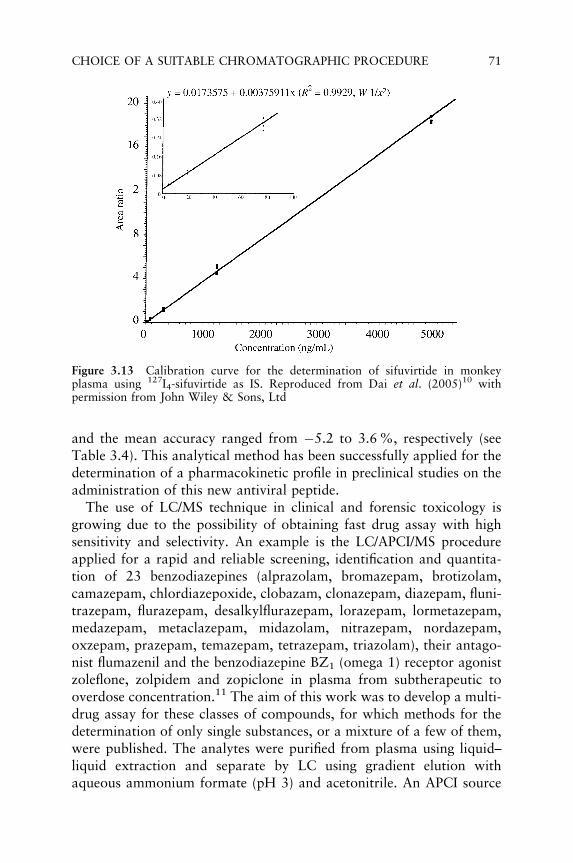
and the mean accuracy ranged from �5.2 to 3.6 %, respectively (seeTable 3.4). This analytical method has been successfully applied for thedetermination of a pharmacokinetic profile in preclinical studies on theadministration of this new antiviral peptide.
The use of LC/MS technique in clinical and forensic toxicology isgrowing due to the possibility of obtaining fast drug assay with highsensitivity and selectivity. An example is the LC/APCI/MS procedureapplied for a rapid and reliable screening, identification and quantita-tion of 23 benzodiazepines (alprazolam, bromazepam, brotizolam,camazepam, chlordiazepoxide, clobazam, clonazepam, diazepam, fluni-trazepam, flurazepam, desalkylflurazepam, lorazepam, lormetazepam,medazepam, metaclazepam, midazolam, nitrazepam, nordazepam,oxzepam, prazepam, temazepam, tetrazepam, triazolam), their antago-nist flumazenil and the benzodiazepine BZ1 (omega 1) receptor agonistzoleflone, zolpidem and zopiclone in plasma from subtherapeutic tooverdose concentration.11 The aim of this work was to develop a multi-drug assay for these classes of compounds, for which methods for thedetermination of only single substances, or a mixture of a few of them,were published. The analytes were purified from plasma using liquid–liquid extraction and separate by LC using gradient elution withaqueous ammonium formate (pH 3) and acetonitrile. An APCI source
Figure 3.13 Calibration curve for the determination of sifuvirtide in monkeyplasma using 127I4-sifuvirtide as IS. Reproduced from Dai et al. (2005)10 withpermission from John Wiley & Sons, Ltd
CHOICE OF A SUITABLE CHROMATOGRAPHIC PROCEDURE 71

was preferred to an ESI one because it is much less susceptible to ionsuppression.12,13 After screening and identification in full-scan mode ofall the analytes, their quantitation was performed by MID analysis. Forquantitative analysis the analytes were divided into four different groupsaccording to their therapeutic range and each group was assigned to oneof four separately recorded traces with specific gain values as given inTable 3.5. The target ions of compounds eluting close to the end of atime window were monitored also in the following time window and, inanalogy, target ions of compounds eluting close to the beginning of atime window were monitored in the respective preceding time window(Table 3.5). This allowed quantification of the respective analytes even ifthe separation line of the time windows was not situated exactlybetween the peaks. For all the compounds the monitored ions were
Table 3.4 Accuracy and precision of sifuvirtide determination in pooled plasmafrom healthy rhesus monkeys at different concentration levels
Concentration (ng/mL)
Group 4.88 19.5 78.1 312.5 1250 5000 Linearity
Day 1 5.5 19.5 83 342 1209 4853 y ¼ A þ Bx4.3 17.4 71 324 1313 5153 A ¼ 0:037485.1 18.6 74 318 1310 4904 B ¼ 0:002107
Mean 4.9 18 76 328 1277 4970 R2 ¼ 0:9939SD 0.6 1.1 6 12 59 161RSD(%) 12.7 5.8 7.8 3.8 4.6 3.2Accuracy(%) 1.3 �5.4 �2.7 5.0 2.2 �0.6Day 2 4.6 18.7 77 301 1229 5235 y ¼ A þ Bx
5.5 17.4 71 323 1275 5078 A ¼ 0:018464.8 18.6 86 296 1391 5124 B ¼ 0:003611
Mean 5.0 18.2 78 307 1298 5146 R2 ¼ 0:9945SD 0.4 0.8 7 14 83 81RSD(%) 9.1 4.2 9.5 4.6 6.4 1.6Accuracy(%) 1.6 �6.6 �0.2 �1.8 3.9 2.9Day 3 5.1 20.9 84 275 1218 4832 y ¼ A þ Bx
4.4 17.8 81 274 1402 5103 A ¼ 0:014875.2 17.7 83 313 1311 5111 B ¼ 0:003985
Mean 4.9 18.8 83 287 1310 5015 R2 ¼ 0:9923SD 0.5 1.8 1.9 22 92 159RSD(%) 9.3 9.8 2.3 7.8 7.1 3.2Accuracy(%) 0.6 �3.6 5.9 �8.1 4.8 0.33-day mean 4.9 18.5 79 307 1295 50443-day SD 0.5 1.2 5.7 23.0 70.3 143.6Total RSD(%) 9.1 6.3 7.2 7.5 5.4 2.8Total accuracy(%) 1.2 �5.2 1.0 �1.6 3.6 0.9
SD, standard deviation; RSD, relative standard deviation.
72 HOW TO IMPROVE SPECIFICITY
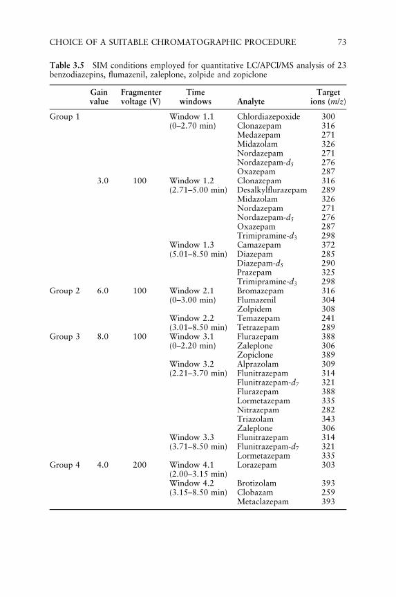
Table 3.5 SIM conditions employed for quantitative LC/APCI/MS analysis of 23benzodiazepins, flumazenil, zaleplone, zolpide and zopiclone
Gain Fragmenter Time Targetvalue voltage (V) windows Analyte ions (m/z)
Group 1 Window 1.1 Chlordiazepoxide 300(0–2.70 min) Clonazepam 316
Medazepam 271Midazolam 326Nordazepam 271Nordazepam-d5 276Oxazepam 287
3.0 100 Window 1.2 Clonazepam 316(2.71–5.00 min) Desalkylflurazepam 289
Midazolam 326Nordazepam 271Nordazepam-d5 276Oxazepam 287Trimipramine-d3 298
Window 1.3 Camazepam 372(5.01–8.50 min) Diazepam 285
Diazepam-d5 290Prazepam 325Trimipramine-d3 298
Group 2 6.0 100 Window 2.1 Bromazepam 316(0–3.00 min) Flumazenil 304
Zolpidem 308Window 2.2 Temazepam 241(3.01–8.50 min) Tetrazepam 289
Group 3 8.0 100 Window 3.1 Flurazepam 388(0–2.20 min) Zaleplone 306
Zopiclone 389Window 3.2 Alprazolam 309(2.21–3.70 min) Flunitrazepam 314
Flunitrazepam-d7 321Flurazepam 388Lormetazepam 335Nitrazepam 282Triazolam 343Zaleplone 306
Window 3.3 Flunitrazepam 314(3.71–8.50 min) Flunitrazepam-d7 321
Lormetazepam 335Group 4 4.0 200 Window 4.1 Lorazepam 303
(2.00–3.15 min)Window 4.2 Brotizolam 393(3.15–8.50 min) Clobazam 259
Metaclazepam 393
CHOICE OF A SUITABLE CHROMATOGRAPHIC PROCEDURE 73

[MþH]þ ionic species, except for brotizolam, clobazam, lorazepam andmetaclazepam due to interferences with other analytes. Differentlabelled ISs have been employed because the use of trimipramine-d3,a typical standard for liquid–liquid extraction of these compounds,14
did not lead to sufficient validation data for all the analytes. Thedifferent IS were assigned to the different analytes in the followingcombination:
� diazepam-d5 for zolpidem, midazolam, lormetazolam, tetrazepamand camazepam;
� flunitrazepam-d7 for zopiclone, bromazepam, flurazepam, desalk-ylflurazepam, oxazepam, lorazepam, nitrazepam and flunitraze-pam;
� nordazepam-d5 for flumazepam, chlordiazepoxide, zaleplone,medazepam, clonazepam, nordazepam, temazepam, brotizolam,metaclazepam, diazepam and prazepam;
� trimipramine-d3 for alprazolam, triazolam and clobazam.
The analytical procedure was validated according to the internation-ally accepted recommendation and interfering peaks due to commondrugs typically taken in combination with analytes could be excludedbasing on their different r.t. values. This is clearly shown in Figure 3.14where typical MID chromatograms of an extract of plasma sample,spiked with IS and the analytes, is reported. The response for all theanalytes was linear from subtherapeutic to overdose concentration(Table 3.6). A weighted (1/c2, where c is the concentration) least-squaresmodel was used for calculation of calibration curves to account for theunequal variances (heteroscedasticity) across the calibration range. Thelow- and high-level recoveries ranged from 87.4 to 113.6 % for all theanalytes but bromazepam. It should be emphasized that all LODsdetermined in full-scan mode were at least equal to the correspondingLOQs in MID mode. The LOQs corresponded to the lowest concentra-tions used for the calibration curves with a signal-to-noise ratio of atleast 10.
This multi-drug assay has proven to be applicable to more than 100authentic plasma samples in daily routine work. As an example, theMID chromatogram obtained from an extract of an authentic plasmasample, analysed for compliance monitoring, is reported in Figure 3.15.As can be seen, well resolved peaks due to oxazepram, lorazepam,nitrazepam and clonazepam were detected: the amount of these analyteswas estimated to be 0.08, 0.01, 0.04 and 0.03 mg/L, respectively.
74 HOW TO IMPROVE SPECIFICITY

Fig
ure
3.1
4Sm
ooth
edand
mer
ged
SIM
chro
mato
gra
ms
norm
ali
zed
wit
hre
spec
tto
the
most
abundant
IStr
imip
ram
ine-
d3
of
abla
nk
pla
sma
extr
act
(a),
of
abla
nk
pla
sma
extr
act
spik
edw
ith
0.2
mg/L
dia
zepam
-d5,
0.0
1m
g/L
flunit
raze
pam
-d7,
0.2
mg/L
nord
iaze
pam
-d5
and
1.0
mg/L
trim
ipra
min
e-d
3(b
)and
of
abla
nk
pla
sma
spik
edw
ith
ISs
and
the
analy
tes
at
ther
apeu
tic
conce
ntr
ati
ons
(c).
Rep
roduce
dfr
om
Kra
tzsc
het
al.
(2004)1
1w
ith
per
mis
sion
from
John
Wil
ey&
Sons,
Ltd

Table
3.6
Ther
apeu
tic
conce
ntr
ati
on
range,
linea
rity
,L
OD
,L
OQ
and
reco
ver
ydata
of
the
LC
/APC
I/M
Sass
ay
for
the
studie
ddru
gs
Ther
apeu
tic
Lim
its
(mg/L
)R
ecover
y
conce
ntr
ati
on
Lin
eari
tyC
oef
fici
ent
of
LO
DL
OQ
Conce
ntr
ati
on
Mea
n�
SD
Dru
gra
nge
(mg/L
)ra
nge
(mg/L
)det
erm
inati
on
(R2)
(sca
nm
ode)
(SIM
mode)
(mg/L
)(%
)
Alp
razo
lam
0.0
05–0.1
20.0
025–0.1
50.9
98
0.0
025
0.0
025
0.0
05
96.0
�2.6
0.1
296.0
�6.2
Bro
maze
pam
0.0
8–0.2
0.0
4–0.2
50.5
51
0.0
10.0
40.0
844.6
�55.1
0.2
39.4
�81.3
Bro
tizo
lam
0.0
01–0.0
30.0
005–0.0
375
0.9
89
0.0
005
0.0
005
0.0
01
104.1
�4.4
0.0
399.4
�5.8
Cam
aze
pam
0.1
–0.6
0.0
5–0.7
50.9
90
0.0
10.0
50.1
104.5
�2.7
0.6
104.1
�6.0
Chlo
rdia
zepoxid
e0.4
–3.0
0.2
–3.7
50.9
96
0.0
10.2
0.4
104.5
�3.1
3.0
102.6
�1.5
Clo
baza
m0.1
–1.2
0.0
5–1.5
0.9
69
0.0
10.0
50.1
87.4
�3.5
1.2
97.6
�6.2
Clo
naze
pam
0.0
1–0.0
50.0
05–0.0
065
0.9
82
0.0
05
0.0
05
0.0
1106.7
�2.1
0.0
597.9
�3.4
Dia
zepam
0.2
–2.0
0.1
–2.5
0.9
92
0.0
10.1
0.2
100.5
�7.3
2.0
98.7
�1.2
Flu
maze
nil
0.0
2–0.1
0.0
1–0.1
25
0.9
91
0.0
10.0
10.0
2102.5
�2.1
0.1
94.9
�3.9
Flu
nit
raze
pam
0.0
1–0.0
30.0
05–0.0
375
0.9
91
0.0
05
0.0
05
0.0
1104.1
�2.3
0.0
399.4
�4.4
Flu
raze
pam
0.0
05–0.1
50.0
025–0.1
875
0.9
93
0.0
025
0.0
025
0.0
05
102.1
�7.5
0.1
591.1
�5.7
Des
alk
ylfl
ura
zepam
0.0
05–0.1
50.0
025–0.1
875
0.9
92
0.0
05
0.0
025
0.0
05
103.9
�7.0
0.1
598.6
�5.5
Lora
zepam
0.0
2–0.2
50.0
1–0.3
125
0.9
97
0.0
20.0
10.0
2101.3
�4.2
0.2
5101.7
�6.7

Lorm
etaze
pam
0.0
01–0.0
30.0
005–0.0
375
0.9
87
0.0
005
0.0
005
0.0
01
101.9
�5.9
0.0
397.9
�4.7
Med
aze
pam
0.0
01–0.0
30.0
005–0.0
375
0.9
87
0.0
005
0.0
005
0.0
01
101.9
�5.9
0.0
397.9
�4.7
Met
acl
aze
pam
0.0
5–0.2
0.0
25–0.2
50.9
92
0.0
25
0.0
25
0.0
5103.0
�2.2
0.2
92.1
�4.2
Mid
azo
lam
0.0
4–0.2
50.0
2–0.5
0.9
96
0.0
05
0.0
20.0
4101.2
�2.3
0.4
99.5
�5.3
Nit
raze
pam
0.0
04–0.2
0.0
02–0.2
50.9
94
0.0
02
0.0
02
0.0
04
98.5
�6.8
0.2
97.9
�4.6
Nord
aze
pam
0.2
–2.0
0.1
–2.5
0.9
91
<0.0
10.1
0.2
103.4
�2.1
2.0
100.7
�4.3
Oxaze
pam
0.0
2–2.0
0.0
1–2.5
0.9
92
0.0
01
0.0
10.0
2104.7
�1.1
2.0
99.6
�5.6
Pra
zepam
0.0
1–2.0
0.0
05–2.5
0.9
95
0.0
01
0.0
05
0.0
193.5
�6.2
2.0
97.6
�5.1
Tem
aze
pam
0.0
2–1.0
0.0
1–1.2
50.9
91
0.0
05
0.0
10.0
2104.9
�1.9
1.0
89.1
�8.1
Tet
raze
pam
0.0
5–0.6
0.0
25–0.7
50.9
93
0.0
05
0.0
25
0.0
5105.1
�2.3
0.6
100.7
�3.6
Tri
azo
lam
0.0
02–0.1
0.0
01–0.1
25
0.9
97
0.0
01
0.0
01
0.0
02
96.0
�6.1
0.1
96.1
�6.7
Zale
plo
ne
0.0
1–0.1
0.0
05–0.1
25
0.9
92
0.0
05
0.0
05
0.0
197.9
�3.8
0.1
99.7
�3.7
Zolp
idem
0.0
8–0.4
0.0
4–0.5
0.9
90
0.0
10.0
40.0
8103.3
�2.4
0.4
104.1
�3.3
Zopic
lone
0.0
1–0.1
50.0
05–0.1
875
0.9
97
0.0
025
0.0
05
0.0
1113.6
�3.5
0.1
5109.8
�11.4
LO
D,
lim
itof
det
ecti
on;
LO
Q,
lim
itof
quanti
tati
on.

Fig
ure
3.1
5Sm
ooth
edand
mer
ged
chro
mato
gra
ms
of
an
extr
act
of
an
auth
enti
cpla
sma
sam
ple
subm
itte
dfo
rco
mpli
ance
monit
ori
ng
indic
ati
ng
0.0
3m
g/L
of
clonaze
pam
,0.0
1m
g/L
of
lora
zepam
,0.0
4m
g/L
of
nit
aze
pam
and
0.0
8m
g/L
of
oxaze
pam
.R
epro
duce
dfr
om
Kra
tzsc
het
al.
(2004)1
1w
ith
per
mis
sion
from
John
Wil
ey&
Sons,
Ltd

3.2 CHOICE OF A SUITABLE IONIZATION METHOD
As described in Chapter 1, different ionization methods are nowadaysavailable and their choice is mainly related to the physico-chemicalproperties of the analytes of interest, as well as to the chromatographicsystem employed for the analyses.
In the case of a complex matrix, it reasonable to assume that it iscomposed of many different classes of compounds, exhibiting physico-chemical and thermodynamic properties different from each other.
These properties can be validly employed to develop a methodexhibiting high selectivity. As discussed in Section 1.1.2, gas-phaseprotonation reactions:
M þ AHþ ! MHþ þ A
take place only if the proton affinity of M is higher than that of A.Consequently, the choice of a suitable reactant AHþ can make possiblethe selective ionization of M, leaving neutral all the molecular specieswith proton affinity values lower than that of A. In other words, it ispossible to use gas-phase protonation by CI experiments to detect onlyanalytes with PA values higher than or equal to that of the reactant A.
This approach becomes more selective in the case of negative ionformation through electron attachment or deprotonation reaction:
M þ e� ! M�:
M þ B� ! ½M � H� þ BH
As an example of the complementarity of the results which can beachieved by the use of different ionization methods, the positive andnegative ion spectra of a secondary metabolite of Aspergillus WentiiWehmer15 (namely 15-acetoxyhexadecylcitraconic anhydride, com-pound 1, Figure 3.16), are reported in Figure 3.17.
Figure 3.16 Structure of 15-acetoxyhexadecylcitraconic anhydride (1)
CHOICE OF A SUITABLE IONIZATION METHOD 79
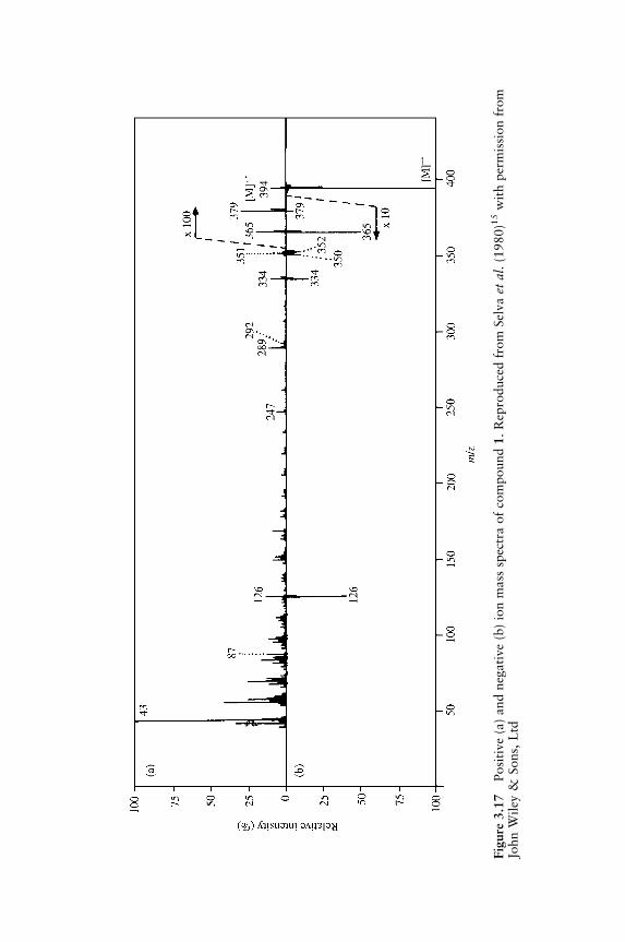
Fig
ure
3.1
7Posi
tive
(a)
and
neg
ati
ve
(b)
ion
mass
spec
tra
of
com
pound
1.
Rep
roduce
dfr
om
Sel
va
etal
.(1
980)1
5w
ith
per
mis
sion
from
John
Wil
ey&
Sons,
Ltd

As can be seen, the positive ion mass spectrum shows diagnostic ionsof very low abundance (the Mþ. species exhibits a relative abundance of0.01 %), while in negative ion mode (obtained by electron attachmentreactions) the M-. species represent the base peak of the spectrum andonly a few fragments (all well related to the molecular structure) aredetectable. This behaviour is in agreement with the high stability of themolecular anions of maleic anhydride derivatives, which can be formedby thermal electron and secondary electron capture, leading to long-lived species by nuclear excited resonance processes, and is also inagreement with the charge localization concept.
This approach can be employed also to obtain a fingerprinting ofmolecules of interest present in complex matrices without the need forchromatographic separation. The data obtained in the identification ofdicarboxylic aciduria, an inborn error of metabolism, are a goodexample of this approach.16 Dicarboxylic aciduria may arise fromseveral inherited or acquired conditions which cause an enzymaticblockage or a metabolitic overflow of mitochondrial b-oxidation ofmedium chain monocarboxylic fatty acid. The biochemical consequenceis a shunt towards a microsomal o-oxidation and synthesis of thecorresponding dicarboxylic acids, particularly sebacic (C10:0), suberic(C8:0) and adipic (C6:0) acids. Figure 3.18 shows the GC/MS profile ofthe urinary organic acids of a 3-year-old boy affected by progressiveneuromuscular deterioration.
The power of NICI(OH�) for a rapid and direct mapping of urinaryorganic acids is shown by the data reported in Figure 3.19. Figure3.19(a) shows the electron impact spectrum of the whole acidic fractionof the sample investigated. Most of the TIC is due to low mass ionic
Figure 3.18 TIC chromatogram of the urinary organic acid extract of a 3-year-oldboy affected by progressive neuromuscular deterioration. Peak 1, succinic acid;peak 2, adipic acid; peak 3, suberic acid; peak 4, sebacic acid. Reproduced fromRinaldo et al. (1985)16 with permission from John Wiley & Sons, Ltd
CHOICE OF A SUITABLE IONIZATION METHOD 81

Fig
ure
3.1
9M
ass
spec
tra
of
the
nonder
ivati
zed
uri
nary
extr
act
leadin
gto
the
chro
mato
gra
mof
Fig
ure
3.1
8obta
ined
under
:(a
)E
Ico
ndit
ions;
(b)
elec
tron
att
ach
men
tco
ndit
ions;
(c)
NIC
I(O
H�
)co
ndit
ions.
Rep
roduce
dfr
om
Rin
ald
oet
al.(1
985)1
6w
ith
per
mis
sion
from
John
Wil
ey&
Sons,
Ltd

species, while no molecular peaks of the dicarboxylic acids are shown.Figure 3.19(b) illustrates the negative ion mass spectrum of the sameurinary fraction, obtained under electron attachment conditions. Mole-cular species of the dicarboxylic moieties are still not detectable, thoughionic species at higher mass value are present. This result can beexplained by the fact that electron attachment underlines molecularspecies with high electron affinity. The abundant ions present in thespectrum (Figure 3.19b) do not correspond necessarily to the molecularspecies present at highest rates in the mixture, but only to moietiesexhibiting the highest electron affinity.
A qualitative profile of the urinary acidic fraction can be clearlyobtained only under hydroxyl negative ion chemical ionization[NICI(OH�)] conditions. Figure 3.19(c) illustrates the forecast [M –H]� species of dicarboxylic acids detected by GC/MS, which are easilydetected (sebacic acid at m/z 201, suberic acid at m/z 173, adipic acid atm/z 145 and succinic acid at m/z 117). In addition, other ions are presentat m/z 89, presumably due to lactic acid.
Summarizing the data shown in Figure 3.19, it follows that:
(i) EI does not lead to any significant results due either to the co-presence of a large number of compounds or to the ineffective-ness of the method in detecting carboxylic acid molecular ions.
(ii) Electron attachment provides evidence of the compounds exhi-biting the highest electron affinity present in urine, but not theacids of interest.
(iii) NICI performed by reaction with gas-phase generated OH�,strongly favours the classic acid–base reaction:
RCOOH þ OH� ! RCOO� þ H2O
with the formation of acid anions.What is observed in analytical methods requiring sample vaporization
(EI and CI) can be transferred to more recently developed ionizationmethods operating with sample solution, in particular in electrosprayconditions.
As an example, the results obtained in the analysis by ESI of a rawextract of artichoke of phytochemical interest are reported in Figure3.20. The electrospray spectrum obtained in positive ion mode is highlycomplex, with peaks practically at every m/z value. Furthermore themost abundant peaks do not correspond to any compound describedamong the main components of the natural extract. In contrast, the
CHOICE OF A SUITABLE IONIZATION METHOD 83

Fig
ure
3.2
0Posi
tive
ion
(a)
and
neg
ati
ve
ion
(b)
ESI
mass
spec
tra
of
ara
wex
tract
of
art
ichoke

negative ion spectrum shows only a few, well defined peaks due tomolecular anions typical of this botanic species.
In all the examples reported above a major point must be emphasized:in negative ion spectra, apart from the identification of structurallydiagnostic ions, a wide decrease in so-called ‘chemical noise’ (i.e. thechemical background due to the presence of many ionic species) isobserved, with a consequent increase in the signal-to noise ratio.
3.3 AN EXAMPLE OF HIGH SPECIFICITY ANDSELECTIVITY METHODS: THE DIOXINANALYSIS
3.3.1 Use of High Resolution MID Analysis
A clear example of the improvement in sensitivity and selectivity, whichcan be obtained by the use of MID in high resolution conditions inquantitative analysis, is the analytical method employed for the deter-mination of polychlorodibenzodioxin (PCDD) and polychlorodibenzo-furan (PCDF) congeners (PCDD/F) in different matrices. The structuresand the list of the toxicologically more relevant PCDD/F are reported inFigure 3.21.
Figure 3.21 Structures of the toxicologically more relevant tetra, penta, hexa,hepta and octa CDD and CDF
AN EXAMPLE OF HIGH SPECIFICITY AND SELECTIVITY METHODS 85

It should be emphasized that this approach fully satisfies the US EPA1613 (Revision B), the European standard EN-1948-1 and the OntarioMinistry of Environment (MOE) methods, all requiring the monitoringof the total concentration of all PCDD/F by high resolution gaschromatography/high resolution mass spectrometry (HRGC/HRMS) atppq levels.
The first problem in this kind of analysis arises from the analyticalsample preparation. The flow chart related to sample treatment isreported in Figure 3.22. Two extraction procedures can be employed,depending on the nature of the substrate of interest (solid or liquid) andthe related results can give an evaluation of extraction procedure.Extraction–purification–separation phases are required and threedifferent labelled standards are introduced in different steps of thepurification treatment:
� IS (15 congeners of 2,3,7,8–13C12 from tetraCDD/F to octaCDD,isotopic purity �99 %);
� purification standard (PS) (2,3,7,8-tetra13C12DD, isotopic purity�96 %);
Figure 3.22 Flow chart of the sample treatment usually employed for PCDD/Fanalysis
86 HOW TO IMPROVE SPECIFICITY

� recovery standard (RS) (1,2,3,4-tetra13C12DD, 1,2,3,7,8,9-Hexa13C12DD, isotopic purity �99 %).
From their levels, it is possible to evaluate the extraction yield.The time scale, reported on the left of Figure 3.22, should be noted:
the whole procedure requires aproximately 22 h!The example reported below concerns the analysis of a certified
sediment, with a total content of PCDD and PCDF of 20042� 4706pg/g. The instrument used was a double focusing mass spectrometer,operating in EI positive ion mode. The instrumental parameters wereaccurately optimized, in order to obtain a mass resolution of 12 000 andthe ions used for the different MID windows are reported in Table 3.7.The electron beam energy employed was 45 eV (instead of thecommonly employed 70 eV).
The TIC chromatogram obtained by full scan analysis is reported inFigure 3.23. As can be seen, the baseline is very high, suggesting thatmany compounds are present in the extract and are not separated by thedeveloped chromatographic procedure. The RIC obtained for the Mþ oftetraCDD (at m/z 320; accurate mass value 319.8965) is reported inFigure 3.24. Taking into account that under the GC conditions used the2,3,7,8-tetraCDD r.t. is 30–31 min, it is impossible to distinguish thetetrachlorodioxin peaks from the background. The same results areobtained for all PCDD/F.
When the GC/MS analysis is carried out under high resolutionMID conditions (Table 3.7), the RIC reported in Figure 3.25 isobtained. A large increase in signal-to-noise ratio is obtained. In theRIC chromatogram based on MID data related to Mþ. ions oftetraCDD, an abundant and well resolved chromatographic peak isobtained at r.t. 30.52 min, as shown in Figure 3.26(a). This peakcorresponds to 2,3,7,8-tetraCDD. The RIC chromatogram related toMþ� ions of 2,3,7,8-tetra13C12DD (used as IS) and of 1,2,3,4-tet-ra13C12DD (used as RS) are reported in Figure 3.26(b). It should beemphasized that in each MID analysis an accurate mass range isapplied in order to determine the ions due to both the analyte andto the corresponding labelled ISs. Once the 2,3,7,8-tetraCDD/ISarea ratio is determined, the calibration curve allows the analyteconcentration in the original sample to be obtained and its recoveryduring the purification procedure to be determined by measuring theIS/RS peak ratio. Analogous results have been obtained for all PCDD/Fcongeners.
AN EXAMPLE OF HIGH SPECIFICITY AND SELECTIVITY METHODS 87

Table 3.7 MID time windows employed in high resolution GC/high resolution MSof PCDD/F
Start End Accurate IonNo. (min) (min) mass identification Compound
303.9016 M TetraCDF305.8987 Mþ 2 TetraCDF315.9419 M Tetra13C12DF (IS or RS)317.9389 Mþ 2 Tetra13C12DF (IS or RS)
1 28.30 34.00 319.8965 M TetraCDD321.8936 Mþ 2 TetraCDD331.9368 M Tetra13C12DD (IS or RS)333.9338 Mþ 2 Tetra13C12DD (IS or RS)354.9792a LOCKa PFKa
339.8598 Mþ 2 PentaCDF341.8569 Mþ 4 PentaCDF351.9000 Mþ 2 Penta13C12DF (IS or RS)353.8970 Mþ 4 Penta13C12DF (IS or RS)
2 34.00 38.00 355.8547 Mþ 2 PentaCDD357.8518 Mþ 4 PentaCDD367.8949 Mþ 2 Penta13C12DD (IS or RS)369.8919 Mþ 4 Penta13C12DD (IS or RS)354.9792a LOCKa PFKa
373.8208 Mþ 2 HexaCDF375.8178 Mþ 4 HexaCDF383.8639 M Hexa13C12DF (IS or RS)385.8609 Mþ 2 Hexa13C12DF (IS or RS)
3 38.00 41.30 389.8156 Mþ 2 HexaCDD391.8127 Mþ 4 HexaCDD401.8559 Mþ 2 Hexa13C12DD (IS or RS)403.8529 Mþ 4 Hexa13C12DD (IS or RS)430.9728a LOCKa PFKa
407.7818 Mþ 2 HeptaCDF409.7788 Mþ 4 HeptaCDF417.8250 M Hepta13C12DF (IS or RS)419.8220 Mþ 2 HeptaCDF
4 41.30 48.00 423.7767 Mþ 2 HeptaCDD425.7738 Mþ 4 HeptaCDD435.8169 Mþ 2 Hepta13C12DD (IS or RS)437.814 Mþ 4 Hepta13C12DD (IS or RS)430.9728a LOCKa PFKa
441.7428 Mþ 2 OctaCDF443.7399 Mþ 4 OctaCDF457.7377 Mþ 2 OctaCDD
5 48.00 55.00 459.7348 Mþ 4 OctaCDD469.7780 Mþ 2 Octa13C12DD (IS or RS)471.7750 Mþ 4 Octa13C12DD (IS or RS)442.9728a LOCKa PFKa
aPFK, perfluorokerosene used as mass calibrant.
88 HOW TO IMPROVE SPECIFICITY

Fig
ure
3:2
3T
ICch
rom
ato
gra
mof
ace
rtifi
edse
dim
ent
wit
ha
tota
lco
nte
nt
of
PC
DD
/Fof
20.0
42�
4.7
06
pg/g

Fig
ure
3.2
4R
ICre
late
dto
Mþ
.of
tetr
aCD
D(m
/z320)
obta
ined
by
elab
ora
tion
of
the
dat
ale
adin
gto
the
TIC
chro
mat
ogr
amof
Fig
ure
3.2
3

Fig
ure
3.2
5M
IDch
rom
ato
gra
mof
the
cert
ified
sedim
ent
extr
act
obta
ined
inhig
hre
solu
tion
condit
ions

Fig
ure
3.2
6R
ICch
rom
ato
gra
m,base
don
the
hig
hre
solu
tion
MID
data
,re
late
dto
Mþ
.io
ns
of
tetr
aC
DD
(a);
the
pea
kdet
ecte
dat
30.5
2m
inco
rres
ponds
to2,3
,7,8
-tet
raC
DD
.R
ICch
rom
ato
gra
mre
late
dto
Mþ
.io
ns
of
2,3
,7,8
-T13C
12D
D(u
sed
as
IS)
and
of
1,2
,3,4
-T13C
12D
D(u
sed
as
RS)
(b)

3.3.2 NICI in the Analysis of Dioxins, Furans and PCBs17
As discussed in Chapter 1, the specificity of a MS method can beincreased by employing selective ionization methods or the MS/MSapproach. These have also been employed in the case of polychlorinateddibenzo-p-dioxins, dibenzofurans and biphenyls.
The power of NICI has been tested by the use of differentreagent gases. In the case of methane, thermal electrons are gene-rated by EI of neutral methane, mainly through two differentmechanisms:
CH4 þ ep ! CHþ:4 þ et þ ep
CH4 þ ep ! CHþ3 þ H: þ et þ ep
where ep represents a primary electron and et is the thermal electronreleased from the methane molecule. The thermal electron interacts withthe neutral molecule M of the analyte, giving rise to an odd electronmolecular anion M�.:
M þ et ! M�::
The yield of these processes is to some extent dependent on experimentalconditions (temperature, ion source type, reactant gas pressure, traces ofoxygen, electron energy, concentration of the analyte), which need to becarefully optimized. Oehme and colleagues18 compared the dataobtained by EI and NICI. Detection limits in the range 0.2–3 pg werefound for 4,6-chlorinated PCDFs, octaCDF, octaCDD, pentaCDD andhexaCDD in NICI conditions, while higher values (3–20 pg) wherefound in EI conditions.
More recently a comparative analysis of dioxins and furans performedby high resolution, electron ionization mass spectrometry and NICI hasbeen carried out by Koester et al.,19 demonstrating the positive andnegative aspects of the two approaches. Comparable detection limitswere obtained (100–200 fg for EI, 50–100 fg for NICI). Other studieshave been carried out using O2, CH4/O2, CH4/N2O, iC4H10/CH2Cl2O2,Ar/CH4, H2, Ar, Xe, SF6, and He as reagent gas. The results obtained,summarized in Table 3.8, have been critically evaluated and comparedby Chernetsova et al.17
AN EXAMPLE OF HIGH SPECIFICITY AND SELECTIVITY METHODS 93

Table 3.8 Detection limits and characteristic ions in NCI mass spectra of PCDDs,PCDFs and PCBs with different reagent gases
Reagent gases PCDDS PCDFS PCBS
CH4 M�, Cl�, [M�Cl]�,[M�2Cl]�, [M-H]�,[M-3Cl]�,[M�4Cl]�,[M�xClþ xH]�
Detection limit10-11–10-14 g(except 2,3,7,8-tetraCDD)
M�, Cl�, [M�2Cl]�,[M�xClþ xH]�
Detection limit10-10–10-13 g
M�, Cl�, [M�Cl]�,[M�2Cl]�,[M�3Cl]�,[M�4Cl]�, [M�H]�,[M�ClþH]�
Detection limit10-12–10-14 g
CH4/O2 M�, [M�ClþO]�,[MþO2�C6H2
Cl2O2]� (m/z 176)Detection limit10-10–10-11 g.Possible todistinguish isomers
M�, [M�ClþO]�,Cl�, [M�ClþH]�
M�, [M-ClþO]�,[M�Cl]�, [M�H]�,Cl�, [M�2Cl]�,[M�ClþH]�,[M�HClþO2]�
O2 M�, [M�ClþO]�
[MþO2
-C6H2Cl2O2]-
(m/z 176)Detection limit10-10–10-12 g.Possible todistinguishisomers
M�, [M�ClþO]�,Cl�
—
O2 (APCI) M�, [M�ClþO]�,[MþO2-C6H2Cl2O2]�
(m/z 176), [M�H]�
Detection limit10-10–10-13 g.Possible todistinguish isomers
[M�ClþO]�, Cl� —
CH4/N2O M�, [MþOH]�,[MþOH-Cl]�,[MþO-Cl]�,[M�Cl]�
Detection limit ca.10-11 g for a fewcompounds.Possible todistinguish isomers
— —
i-C4H10//CH2Cl2/O2
[M�ClþO]�
Detection limit ca.10-10 g withoutpreliminary GCseparation
[M�ClþO]�
Detection limit ca.10-10 g withoutpreliminary GCseparation
[M�ClþO]�
Detection limit ca.10-10 g withoutpreliminary GCseparation
94 HOW TO IMPROVE SPECIFICITY

3.3.3 MS/MS in the Determination of Dioxins, Furans andPCBs20
The selectivity by high resolution MS and NICI can be reached alsoby MS/MS experiments. In an early paper by March et al., a rapidscreening technique, based on the MS/MS approach by an ion trap, was
Ar/CH4 M�, Cl�, [M�Cl]�,[M�2Cl]�,[MþH�Cl]�,[M�3Cl]�
Detection limit ca.10�12–10�14 g
— —
H2 M�, [M-Cl]�, Cl�;[M-ClþO]�
(in presence of O2)Detection limit ca.10-12 g for a fewcompounds
— —
He M�, Cl�, [M�Cl]� — —Ar M�, Cl�, [M�Cl]� — —Xe M�, Cl� — —SF6 Cl� — —NH3 — — M�, Cl�, [M�Cl]�,
[M�2Cl]�,[M�3Cl]�,[M�4Cl]�,[M�ClþH]�
Detection limit10-12–10-14 g
Ar/O2 — — M�, [M-ClþO]�,[M�HClþO2]�
When the numberof chlorine atoms <4,the sensitivity is betterthan using CH4/O2
CH4/H2O — — M�, [M�ClþO]�,[M�HClþO2]�
When the number ofchlorine atoms >4,the sensitivity is betterthan using CH4/O2
Table 3.8 (Continued)
Reagent gases PCDDS PCDFS PCBS
AN EXAMPLE OF HIGH SPECIFICITY AND SELECTIVITY METHODS 95

reported for the investigation and quantitative analysis of tetraCDD.21
Figure 3.27 shows the chromatograms obtained by high resolution MSand by ion trap MS/MS experiments. The former originated by the ionsignal obtained in SIM mode for m/z value 321.8936 ([Mþ 2]þ. speciesof molecular ion), while the latter is due to the signal of the collision-ally generated ion at m/z 259 (originating from a primary COCl. loss).The two chromatograms are practically superimposable, indicatingthat the possible differences in critical energies related to the COCl.
loss from the different isomers does not affect the quantitative mea-surements.
The ion traps currently available allow multiple reaction monitoring(i.e. select different ions to be subjected to further collisions) to beperformed and consequently product ions from tetra- to octaCDDs/CDFs can be monitored in a single chromatographic acquisition.
The scan function (i.e. the graphical representation of the variation ofthe potentials applied on the ion trap electrodes with respect to time)employed for MS/MS quantitative analysis of tetraCDD22 is shown inFigure 3.28. The main RF voltage (applied on the ring electrode) isincreased, to eject from the ion trap all ions with m/z values lower than160. In order to avoid space-charge effects a first ionization stage (200 ms)is applied: it allows the optimum duration of the real ionizationphase, which was always lower than 20 ms, to be determined. At thisstage, all ions are trapped inside the device and by the application of a
Figure 3.27 Two chromatograms for tetraCDDs obtained from a clam extract.(a) The chromatogram has been obtained in high resolution MID conditions for theMþ. ions at m/z 321.8936; (b) the chromatogram was obtained by monitoring theproduct ion signal (m/z 259) obtained by collision of the Mþ. ions. Reproduced fromMarch et al. (2000)21 with permission from Elsevier
96 HOW TO IMPROVE SPECIFICITY

RF ramp (on the ring electrode) and of a broadband waveform (on thetwo end cap electrodes) all the ions with m/z values lower than 320 andhigher than 322 are ejected from the trap. In these conditions Mþ. and[Mþ 2]þ. ions of tetraCDDs are the only ions present inside the trap.The application of a supplementary RF voltage on the two end caps withresonance frequency corresponding to the ions at m/z 320 and 322 leadsto the activation of collisional phenomena of these ions with the Heatoms present in the trap as buffer gas. The collisionally induceddecomposition products are then ejected from the ion trap by increasingthe main RF voltage and detected.
The scan function can be rapidly changed during the chromatographicrun, so that different ions can be selected, decomposed and the relateddecomposition product ions detected.
The TIC of the mixture described in Table 3.9, is reported inFigure 3.29.22 (The diamonds on the abscissa indicate the change ofscan function.) The peak number–compound correspondence is
Figure 3.28 Scan function employed for MS/MS of tetraCDD. Reproduced fromSplendore et al. (1997)22 with permission from Elsevier
AN EXAMPLE OF HIGH SPECIFICITY AND SELECTIVITY METHODS 97
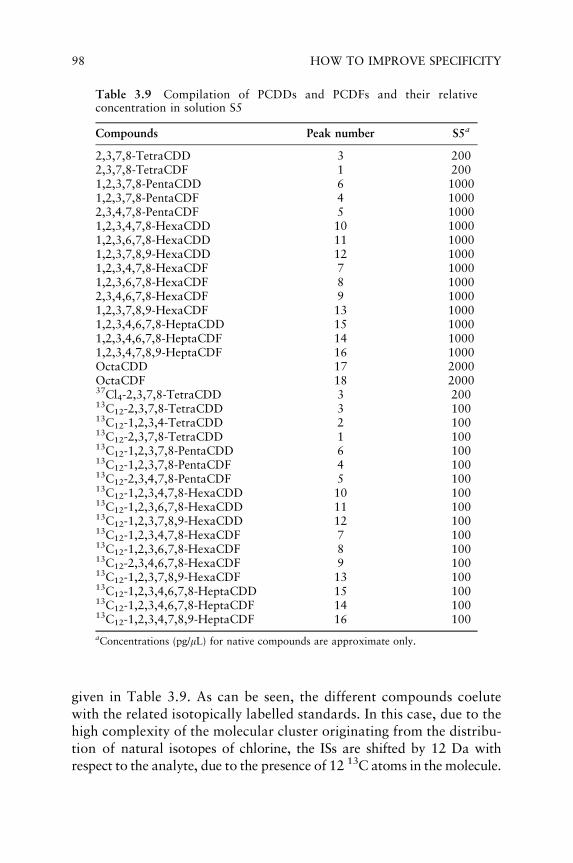
given in Table 3.9. As can be seen, the different compounds coelutewith the related isotopically labelled standards. In this case, due to thehigh complexity of the molecular cluster originating from the distribu-tion of natural isotopes of chlorine, the ISs are shifted by 12 Da withrespect to the analyte, due to the presence of 12 13C atoms in the molecule.
Table 3.9 Compilation of PCDDs and PCDFs and their relativeconcentration in solution S5
Compounds Peak number S5a
2,3,7,8-TetraCDD 3 2002,3,7,8-TetraCDF 1 2001,2,3,7,8-PentaCDD 6 10001,2,3,7,8-PentaCDF 4 10002,3,4,7,8-PentaCDF 5 10001,2,3,4,7,8-HexaCDD 10 10001,2,3,6,7,8-HexaCDD 11 10001,2,3,7,8,9-HexaCDD 12 10001,2,3,4,7,8-HexaCDF 7 10001,2,3,6,7,8-HexaCDF 8 10002,3,4,6,7,8-HexaCDF 9 10001,2,3,7,8,9-HexaCDF 13 10001,2,3,4,6,7,8-HeptaCDD 15 10001,2,3,4,6,7,8-HeptaCDF 14 10001,2,3,4,7,8,9-HeptaCDF 16 1000OctaCDD 17 2000OctaCDF 18 200037Cl4-2,3,7,8-TetraCDD 3 20013C12-2,3,7,8-TetraCDD 3 10013C12-1,2,3,4-TetraCDD 2 10013C12-2,3,7,8-TetraCDD 1 10013C12-1,2,3,7,8-PentaCDD 6 10013C12-1,2,3,7,8-PentaCDF 4 10013C12-2,3,4,7,8-PentaCDF 5 10013C12-1,2,3,4,7,8-HexaCDD 10 10013C12-1,2,3,6,7,8-HexaCDD 11 10013C12-1,2,3,7,8,9-HexaCDD 12 10013C12-1,2,3,4,7,8-HexaCDF 7 10013C12-1,2,3,6,7,8-HexaCDF 8 10013C12-2,3,4,6,7,8-HexaCDF 9 10013C12-1,2,3,7,8,9-HexaCDF 13 10013C12-1,2,3,4,6,7,8-HeptaCDD 15 10013C12-1,2,3,4,6,7,8-HeptaCDF 14 10013C12-1,2,3,4,7,8,9-HeptaCDF 16 100
aConcentrations (pg/mL) for native compounds are approximate only.
98 HOW TO IMPROVE SPECIFICITY

Thus, peak 1 is due to 2,3,7,8-tetraCDF and its coeluting 13C-labelledisotopomer and consequently two different scan functions must beactivated.
Typical data obtained by this approach are show in Figure 3.30,in which the marked tailing of the octachlorodioxin (peak 17 ofFigure 3.29) and furan (peak 18 of Figure 3.29) are reported.22 Theselected ion chromatograms are related to the isolated molecular ionsignal intensities (before any collision) in Figure 3.30(b) and to thefragment ion signal intensities obtained by collision in Figure 3.30(a)(see the related MS/MS spectra in the Figure).
An extensive comparison of the results obtained for the determina-tion of PCDD/F by high resolution GC/high resolution MS, MS/MSexperiments by both QQQ and MS/MS performed by ion traphas been reported in the literature.20 In general, the high resolutionGC/high resolution MS detection limit was lower than those of QQQand ion trap, as shown in Figure 3.31. However, evidence wasfound that all interferences are not eliminated in high resolutionGC/high resolution MS conditions and consequently MS/MS is ofhigh interest.
Figure 3.29 TIC chromatogram obtained after the mass spectrum mergingprocedure for PCDD/F contained in 1 mL of solution S5. The peak identificationis given in Table 3.9. Reproduced from Splendore et al. (1997)22 with permissionfrom Elsevier
AN EXAMPLE OF HIGH SPECIFICITY AND SELECTIVITY METHODS 99

Figure 3.30 Unmerged ion chromatograms for three co-eluting octachlorinatedcompounds. Each chromatogram is composed of the signal intensities of the ionicspecies identified on the ordinate. (a) The fragment ion signal intensities wereobtained by collisional spectra, and one such mass spectrum is displayed for eachcompound. (b) The isolated molecular ion signal intensities were obtained prior tocollision, and a mass spectrum that shows the isolated molecular ions is displayedfor each compound. Reproduced from Splendore et al. (1997)22 with permissionfrom Elsevier
100 HOW TO IMPROVE SPECIFICITY

3.4 AN EXAMPLE OF MALDI/MS IN QUANTITATIVEANALYSIS OF POLYPEPTIDES: SUBSTANCE P
As described in Chapter 1, MALDI favours the formation of molecularspecies ([MþH]þ, [M-H]�) and is particularly effective for the MSanalysis of macromolecules, either from synthesis (polymers) or fromnatural substrates (proteins, oligonucleotides, polysaccharides).
Figure 3.31 Ion signals obtained with each instrument for low concentrations of2,3,7,8-tetraCDD: (a) high resolution conditions, 0.5 pg injected, the signal intensitysum due to m/z 320 and 322 is shown; (b) triple quadrupole, 1.0 pg injected, thesignal intensity sum due to m/z 257 and 259 is shown; (c) ion trap, 0.5 pg injected,the signal intensity sum due to m/z 257, 259, 194 and 196 is shown. The signal-to-noise ratios are approximately 30 in the first case, 50 in the second and 15 in thelast one. Reproduced from March et al. (2000)21 with permission from Elsevier
AN EXAMPLE OF MALDI/MS IN QUANTITATIVE 101

As emphasized in Chapter 1, the mechanisms through which mole-cular species are generated are quite complex, based on both physicaland chemical phenomena strongly reflected in the spectrum quality. Forthese reasons the use of MALDI for quantitative analysis seemed to be,in principle, practically impossible. However, recently some papers haveappeared on MALDI application for quantitative analysis of biologicallyrelevant polypeptides in a complex matrix, proving that, once accurateset-up of the different instrumental parameters has been performed,valid quantitative data can be obtained.
As an example of this approach, we report here the data obtained inthe analysis of Substance P (SP) in rat brain.23
SP (Figure 3.32) is a peptide neurotransmitter distributed in theperipheral and central nervous system, where it acts as a neuromodu-lator. Abnormal levels of SP are associated with disorders such asschizophrenia and Huntington’s, Parkinson’s and Alzheimer’s diseases.Its presence in a variety of tissues and its participation in variousdiseases make the quantitative analysis of SP extremely relevant.
MALDI/TOF MS has become a valuable and important analyticaltool in biological research owing to its ability to analyse low concentra-tions of peptides and proteins in complex biological mixtures and it hasbeen employed in the development of a quick method for detecting anddetermining the SP level in rat brain tissue using a-cyano-4-hydroxycin-namic acid (HCCA) as matrix. The method is based on analysing the SPlevel in the rat brain by immunoprecipitation, in which the SP polyclonalantibodies are raised, followed by solid phase extraction. The levels ofSP were determined by measuring the abundance of [MþH]þ ions byusing the calibration curves constructed by external standards. Theinfluence of the laser on the signal intensities and sample preparationtechniques including flight time deviation for accurate mass measure-ments were evaluated. In combination with MALDI/MS, CZE analyseswere also performed and the results obtained by the two analyticalapproaches were compared.
Due to the complex biological fluid mixtures (brain tissue extracts), itwas necessary to isolate low concentrations of the analyte of interestfrom the biological fluid prior to the MALDI/MS analysis. Immunoaffi-nity capture of the analyte from the biological mixture is a method thatpre-concentrates the analyte and provides the most selective form ofanalyte isolation.24 High affinity polyclonal SP antibodies were used tospecifically purify and enrich the SP. During incubation the SP wascaptured on the antibody, and after a series of washes the immun-oprecipitated samples were subjected to a MALDI sample preparation
102 HOW TO IMPROVE SPECIFICITY

Fig
ure
3.3
2Str
uct
ure
of
Subst
ance
P.
Rep
roduce
dfr
om
Babu
etal
.(2
004)2
3w
ith
per
mis
sion
from
Els
evie
r

step. MS analysis of the immunoprecipitated sample confirmed thepresence of SP for the detection of the related [MþH]þ species atm/z 1348.8.
The laser power was found to be an important parameter, stronglyaffecting the peak [MþH]þ intensity. MS analyses were performed withdifferent laser power, ranging from the minimum intensity necessary forsignal production to the maximum intensity, which was very close to thedetector saturation. Through a series of experiments using SP concen-tration ranging from 50 to 250 fmol/mL, the laser intensity was set to theinitial minimum energy and further increased until an acceptable andwell reproducible signal was obtained.
In order to maximize the signal quality and reproducibility, the laserintensity, the sample preparation methods, the crystallization processand the m/z ranges were carefully adjusted. Ten samples were preparedfor different HCCA/analyte combination. Every mass spectrum wasrecorded as the sum of 40 consecutive spectra collected from a selectedspot on the probe tip and the average peak intensity values were takenfor analysis.
Using this instrumental parameterization, the system was calibratedusing angiotensin II (Ang II) and ACTH fragment 18-39 (ACTH) asexternal standards to normalize the SP [MþH]þ peak intensities. Forthis, a working curve was a first generated for these external standards.Singly charged Ang II and ACTH [MþH]þ ion peak intensities wereused to generate the curve. Regression analysis resulted in the followinglinear equations:
y ¼ 516:4x þ 121:73 ðAng IIÞy ¼ 560:17x þ 79:32 ðACTHÞ
with correlation coefficients of 0.9988 (Ang II) and 0.9899 (ACTH),respectively, where x is the Ang II and ACTH concentrations and y theanalyte peak intensity.
The SP working curves were constructed for a standard SP concentra-tion series by measuring the peak height mass spectral response as afunction of SP concentration. Angiotensin II, ACTH (1 pmol/mL each)and different SP concentrations (from 0.5 to 20 pmol/mL) were premixedwith the matrix. SP [MþH]þ peak intensity for the different SPconcentrations was normalized to the ([Ang IIþH]þþ [ACTHþH]þ)peaks, and the normalized response was plotted as a function of the SPconcentration. The SP working curve response (Figure 3.33) followed alinear relationship (y ¼ 0:1144x þ 0:2145) over the concentration range
104 HOW TO IMPROVE SPECIFICITY

used with a correlation coefficient of 0.9988 and a 0.74 % relativestandard deviation.
The immunoprecipitated samples (A and B) from brain tissue weresubjected to MS analysis, and, as mentioned earlier, the mass spectrumwas acquired at fixed MALDI conditions. The singly charged [MþH]þ
ion peak corresponding to the SP molecular mass was observed. The SPconcentrations were determined in the brain tissue extracts from twoindividuals and are reported in Table 3.10, together with the dataobtained for the same sample by CZE (ultraviolet detection), showinggood agreement between the results achieved by the two techniques.
Table 3.10 MALDI/MS and CZE quantification of SP in the ratbrain
Substance P (pmol/mg protein)
Immunoprecipitated MALDI/MS CZEsamples (n ¼ 10) (n ¼ 3)
A 0.12� 0.06 0.23� 0.04B 0.36� 0.05 0.38� 0.02
Protein concentration (mg/mL): sample A¼ 2.495; sample B¼ 2.201.
Figure 3.33 SP calibration curve. [SPþH]þion peak intensity (normalized to[MþH]þ peak intensity of angiotensin II and ACTH) versus SP concentration.Reproduced from Babu et al. (2004)23 with permission from Elsevier
AN EXAMPLE OF MALDI/MS IN QUANTITATIVE 105

REFERENCES
1. A. Braithwaite and F. J. Smith in Chromatographic methods, 4th Edition, Chapman
and Hall, New York (1985).
2. L. R. Snyder and J. J. Kirkland in Introduction to Modern Liquid Chromatography,
2nd Edition, John Wiley & Sons, Inc., New York (1979).
3. M. Khaledi (Ed.) High Performance Capillary Electrophoresis: Theory, Techniques
and Applications, John Wiley & Sons, Inc., New York (1998).
4. R. M. Smith (Ed.) Supercritical Fluid Chromatography, The Royal Society of
Chemistry, London (1989).
5. A. Lapolla, R. Flamini, T. Tonus, D. Fedele, A. Senesi, R. Reitano, E. Marotta, G. Pace,
R. Seraglia and P. Traldi, Rapid Commun. Mass Spectrom., 17, 876–878 (2003).
6. R. Flamini, G. De Luca and R. Di Stefano, Vitis, 41, 107–114 (2002).
7. G. De Revel and A. Berthirand, J. Sci. Food Agric., 61, 267–272 (1993).
8. A. Lapolla, R. Flamini, A. Dalla Vedova, A. Senesi, R. Reitano, D. Fedele, E. Basso, R.
Seraglia and P. Traldi, Clin. Chem. Lab. Med., 41, 1166–1173 (2003).
9. J. D. Henion and G. A. Maylin, Biomed. Mass Spectrom., 7, 115–121 (1980).
10. S. Dai, H. Song, G. Dou, X. Qian, Y. Zhang, Y. Cai, X. Liu and Z. Tang, Rapid
Commun. Mass Spectrom., 19, 1273–1282 (2005).
11. C. Kratzsch, O. Tenberhen, F. T. Peters, A. A. Weber, T. Kraemer and H.H. Maurer,
J. Mass Spectrom., 39, 856–872 (2004).
12. H. H. Maurer, C. J. Schmitt, A. A. Weber and T. Kraemer, J. Chromatogr.B, 748,
125–135 (2000).
13. K. A. Mortier, K. M. Clauwaert, W. E. Lambert, J. F. Bocxlaer, E. G. Van den
Eeckhout, C. H. Van Peteghen and A. P. De Leenheer, Rapid Commun. Mass
Spectrom., 15, 1773–1775 (2001).
14. H. H. Maurer in Mass Spectral and GCData of Drugs, Poisons, Pesticides, Pollutants
and their Metabolites, Part 4, K. Pfleger, H. H. Maurer and A. Weber (Eds), John
Wiley & Sons, Ltd, Weinheim (2000).
15. A. Selva, P. Traldi, L. Camarda and G. Nasini, Biomed. Mass Spectrom., 7, 148–152
(1980).
16. P. Rinaldo, G. Miolo, L. Chiandetti, F. Zacchello, S. Daolio and P. Traldi, Biomed.
Mass Spectrom., 12, 570–576 (1985).
17. E. S. Chernetsova, A. I. Revelsky, I. A. Revelsky, I. A. Mikhasenko and T.G.
Sobolevsky, Mass Spectrom. Rev., 21, 373–387 (2002).
18. M. Oehme, S. Manø, A. Mikalsen and P. Kirschmer, Chemosphere, 15, 607–617
(1986).
19. C. J. Koester, R. L. Harless and R. H. Hites, Chemosphere, 24, 421–426 (1992).
20. J. B. Plomley, H. Lausevic and R. E. March, Mass Spectrom. Rev., 19, 305–365
(2000).
21. R. E. March, M. Splendore, E. J. Reiner, R. S. Mercer, J. B. Plomley, D. S. Waddell
and K. A. McPherson, Int. J. Mass Spectrom. Ion Processes, 197, 283–297 (2000).
22. M. Splendore, J. B. Plomley, R. E. March and R. S. Mercer, Int. J. Mass Spectrom.
Ion Processes, 165/166, 595–609 (1997).
23. C. V. S. Babu, J. Lee, D. S. Lho and Y. S. Yoo, J. Chromatogr. B, 807, 307–313 (2004).
24. R. W. Nelson, J. S. Krone, A. C. Bieber and P. Williams, Anal. Chem. 67, 1153–1158
(1995).
106 HOW TO IMPROVE SPECIFICITY

4Some Thoughts on Calibration
and Data Analysis
Quantitative analysis and estimation of detection limits in the concen-tration domain require, in general, a previous calibration step. Thereforein this chapter we will describe and discuss thoroughly the calibrationprocedure and we will adapt it, following statistical arguments, to theproblem of the determination of the critical level LC, of the limit of detec-tion LD and of the limit of quantification LQ.1–7 We here will mainlyrefer to the papers of Gibbons and colleagues8 and of Schwartz9–10 forthe definitions and the calculation procedure adopted.
As outlined in Chapter 2, the samples used in the calibration design inGC/MS analysis are solutions at various known concentrations of theanalyte and at constant known concentration of the IS. Consequently,the dependent variable y in the calibration plot is the ratio of the analyteand of the IS responses, and the independent variable x is the knownconcentration ratio. This procedure is valid under the basic assumptionthat the error in response ratio is greater than that in the concentrationratio of the standard solutions. Otherwise, the reverse, a regression ofconcentration ratios on the response ratios, must be carried out.
We will treat both straight line and quadratic models since a curvaturein the calibration plot can arise for two main reasons:11 a large dynamicrange and the eventual use of an IS of type A, isotopically labelledcompound. It is well known that, in the case of a not isotopically purestandard, the curve of the isotope ratio (ratio of the ion current observedfor the unlabelled species to that of the labelled species) versus the molar
Quantitative Applications of Mass Spectrometry I. Lavagnini, F. Magno, R. Seraglia and P. Traldi
# 2006 John Wiley & Sons, Ltd

ratio (ratio of the unlabelled to labelled compounds) is theoreticallycurvilinear.12
The same two reasons imply very often the non constant variance ofthe response ratios at different concentration ratios.13 Consequentlyordinary least-squares regression must be substituted for weighted least-squares procedure, where the inverse of the variance is used as weightingfactor.
4.1 CALIBRATION DESIGNS
It is noteworthy to outline that the calibration design used for theestimation of detection limits can be quite different1,2,5 from that usedfor a quantitative analysis. In the former case the known concentrationsof the spiked solutions must be in the range of the hypothesizeddetection limit, whereas in the latter the standard solutions must bracketthe unknown concentration. In particular, some authors suggest that theblank solution response must be inserted in the regression procedurewhen the detection limits are required. It is common opinion that thenumber of suitably spaced calibration points can range between sevenand ten to obtain a reliable model for the calibration line1,6,8 and thatthe basic pattern must be repeated several times, at least eight to tenreplicates7,14 to gain information about the overall variances of theresponses at the various concentrations. This requirement is due to thefact that a considerable source of variability is always the preparation ofthe sample and of the calibration solutions.
4.2 HOMOSCEDASTIC AND HETEROSCEDASTICDATA
Ordinary least squares (OLS) regression is used with data of uniformvariance, the homoscedastic case, whereas weighted least squares (WLS)regression is appropriate under heteroscedastic conditions to draw theright model from the calibration data. It is known that WLS does notgreatly affect the parameter estimates but it has a deep effect on theestimates of the precision and consequently on the detection limitestimate.9 To verify whether homoscedasticity or heteroscedasticityexists two approaches can be followed: (i) Bartlett’s test is done tocompare the variances of the replicates at different concentrationlevels;15 (ii) the plot of residuals fitting an unweighted least squares
108 SOME THOUGHTS ON CALIBRATION AND DATA ANALYSIS

line versus predicted values is examined. A funnel shape indicates anincreasing variability with increasing response magnitude, i.e. withconcentration. A more immediate analysis of the uniformity of theexperimental variances with concentration is simply the plot of thedifferences of each replicate from the mean of the replicates at eachconcentration. Values close to zero indicate uniformity in the variance.
4.2.1 Variance Model
In the case of heteroscedasticity it is profitable to plot the experimentalvariances s2 or the standard deviations s versus the concentration c andto calculate by regression the relative model. The availability of therelationship s2=c will be very useful in the weighted regression analysis,in the calculation of detection and quantification limits and in general inthe operation of inverse regression (see Section 4.3.1.2). Different typesof s2 function of concentration can be evaluated. Common models are:s2 depending on c via a linear or a quadratic model; s2 changing with c inan exponential way.
A recent paper7 claims, on the basis of numerous experiments inatomic absorption spectroscopy, GC/MS and inductively coupledplasma mass spectrometry, that the measurement error of an analyticalmethod is of two types: constant at very low concentration; propor-tional to the concentration at higher concentration. Consequently thevariance of the response is represented as s2 ¼ a0 þ a1c2.
4.3 CALIBRATION MODELS
The more popular model is always the straight line independent ofscedasticity. Sometimes nonlinear calibration relationships have to beused, in particular when a wide dynamic range is explored. In this case,simple quadratic functions are completely satisfactory. Depending onthe test of scedasticity the unweighted or the weighted regressionprocedure is followed.
4.3.1 Unweighted Regression
In this section we describe a least squares univariate regression analysisof response y on the analyte concentration x using a linear, first-order
CALIBRATION MODELS 109

model (straight line):
y ¼ b0 þ b1x þ e ð4:1Þ
and a linear, second-order model (quadratic model):
y ¼ b0 þ b1x þ b2x2 þ e ð4:2Þ
The independent variable x is assumed unaffected by error, b0, b1, andb2 are the parameters of the model and e represents a normallydistributed random error, with mean zero and constant variances2; e � Nð0; s2Þ. The signal, therefore, is thought to be composed of adeterministic component predictable by the model and a randomcomponent e. Figure 4.1 illustrates the assumptions concerning e inthe case of a straight line. The b parameters are unknown and the leastsquares regression furnishes their estimates by using a set of experi-mental data points ðxi; yiÞ. Thus we write:
yy ¼ b0 þ b1x ð4:10Þ
or
yy ¼ b0 þ b1x þ b2x2 ð4:20Þ
y = b0 + b1 x
Concentration
Res
pons
e
Figure 4.1 Model for linear regression in the homoscedastic case, showingdistributions of measurements around the true calibration line
110 SOME THOUGHTS ON CALIBRATION AND DATA ANALYSIS

where yy represents the predicted response of y for a given x.It is common practice to use software packages to calculate estimates
of the parameters and any other statistics of interest but we here reportalso the explicit formulas for any cases treated.
4.3.1.1 Straight Line Calibration Curve
The least squares estimates of parameters and of their variances inEquation (4.10) are given by:
b0 ¼ �yy � b1�xx ð4:3Þ
b1 ¼
Pn1
iðxi � �xxÞyi
Pn1
iðxi � �xxÞ2ð4:4Þ
s2b0
¼ s2y=x
1
nþ �xx2
Pn1
iðxi � �xxÞ2
2664
3775 ð4:5Þ
s2b1
¼s2y=xPn
1iðxi � �xxÞ2
ð4:6Þ
s2y=x ¼
Pn1
iðyi � yyiÞ2
n � 2ð4:7Þ
where n is the overall data point number:
n ¼Xk
1
jmj
k is the number of the concentration levels and mj is the number ofreplicates at the level j
�xx ¼
Pn1
ixi
n
�yy ¼
Pn1
iyi
n
CALIBRATION MODELS 111

and s2y=x is the residual variance of the regression. It represents an
estimate of the error variance s2 if the model is correct.The adequacy of the model can be tested in several ways:16
(i) by the evaluation of the correlation coefficient
r ¼ n�xy � �x�y
½n�x2 � ð�xÞ212½n�y2 � ð�yÞ2
12
;
(ii) by the use of the lack of fit test;(iii) by inspection of the behaviour of the residuals versus concentra-
tion.
The first procedure is to be discouraged as it can lead to misinterpreta-tion, the second one requires a good number of data points; the third isgraphical in nature, easy to do and very revealing as to whether theassumptions on the errors e and the model are correct.
4.3.1.2 Discrimination
The analytical application of the calibration curve is always thediscrimination, i.e. obtaining x from an analytical response y, x ¼ðy � b0Þ=b1. The degree of uncertainty on x depends on two factors:the uncertainty associated with the estimates b0 and b1, which impliesthe nonuniqueness of the regression line; and the uncertainty associatedwith the experimental response reading. A common way to take intoaccount these two sources of error for x is the use of the ð1 � aÞ100%two-sided prediction intervals whose limits are:
y ¼ b0 þ b1x tð1�a=2; n�2Þsy=x 1 þ 1
nþ ðx � �xxÞ2
Pn1
iðxi � �xxÞ2
2664
3775
1=2
ð4:8Þ
where tð1�a=2;n�2Þ is ð1 � a=2Þ100 percentage point of Student’s t-dis-tribution on n � 2 degrees of freedom.17 Equation (4.8) refers to a singley reading but, if the average �yym of m replicates y1; y2; . . . ; ym isconsidered, it changes into:
�yy ¼ b0 þ b1x tð1�a=2; n�2Þsy=x1
mþ 1
nþ ðx � �xxÞ2
Pn1
iðxi � �xxÞ2
2664
3775
1=2
ð4:9Þ
112 SOME THOUGHTS ON CALIBRATION AND DATA ANALYSIS

When m is very large, m ! 1, Equation (4. 9) collapses to:
y ¼ b0 þ b1x tð1�a=2;n�2Þsy=x1
nþ ðx � �xxÞ2
Pn1
iðxi � �xxÞ2
2664
3775 ð4:10Þ
which is usually called the ð1 � aÞ100% regression band.The real significance of Equations (4.8)–(4.10) is as follows: at a fixed
x, the intervals whose limits are given by these equations contain theresponse y, �yym, �yym!1, respectively, with probability 1 � a. Figure 4.2shows the prediction and the regression bands relative to the three casesillustrated. At this point, given an y0 value, we are able to calculate thecorresponding x0 and its limits of confidence x�
0 , xþ0 . In Figure 4.3 two
graphical procedures used to calculate x0, x�0 and xþ
0 are shown. In thefirst case, the discrimination interval ðx�
0 ; xþ0 Þ is obtained by intersecting
the two-sided prediction interval with a straight line y ¼ y0 (Figure4.3a). This definition of the interval relies on the fact that we accept aslimits for x0, values of x whose relevant predicted values exhibit
Figure 4.2 Ordinary least squares regression analysis: the middle line is thecalibration line, the bounding lines are the regression bands (plots of Equation 4.10)and prediction intervals (plots of Equation 4.8 and Equation 4.9 with m ¼ 8)
CALIBRATION MODELS 113

y0
y0
X0- X0 X0
+
X0- X0 X0
+
Concentration
Res
pons
eR
espo
nse
Concentration
(a)
(b)
Figure 4.3 (a) The y ¼ y0 line comprises the graphical solution for confidencelimits of the discriminated value x0 by intersecting the prediction intervals. (b) Aconfidence interval on the response axis is converted into a discrimination intervalon the x axis by observing where it intersects the confidence band on the regressionline
114 SOME THOUGHTS ON CALIBRATION AND DATA ANALYSIS

ð1 � aÞ100% prediction intervals with the experimental response y0 asthe upper and the lower limits. Alternatively in Figure 4.3(b) theð1 � aÞ100% confidence interval for x0 is obtained by intersectingthe ð1 � a=2Þ100% confidence interval of y0 with the two-sidedð1 � a=2Þ100% regression band (Equation 4.10) on y ¼ b0 þ b1x andprojecting the intersections onto the x axis.18 The basic idea of thissecond approach is that all the points of the shaded area have coordi-nates belonging jointly to the confidence intervals of y0 and of theregression line. In both cases the graphical procedures can be replacedby the analytical approach.
Referring to Figure 4.3(a), the limits x�0 , xþ
0 are obtained as solution ofthe equations:
y0 ¼ b0 þ b1x�0 þ tð1�a=2; n�2Þsy=x
1
mþ 1
nþ ðx�
0 � �xxÞ2
Pn1
iðxi � �xxÞ2
2664
3775
1=2
ð4:11aÞ
y0 ¼ b0 þ b1xþ0 � tð1�a=2; n�2Þsy=x
1
mþ 1
nþ ðxþ
0 � �xxÞ2
Pn1
iðxi � �xxÞ2
2664
3775
1=2
ð4:11bÞ
Referring to Figure 4.3(b), the limits x�0 , xþ
0 are calculated using theequations:
y0 þ tð1�a=4;m�1Þsy0¼ b0 þ b1xþ
0
� tð1�a=4; n�2Þsy=x1
nþ ðxþ
0 � �xxÞ2
Pn1
iðxi � �xxÞ2
2664
3775
1=2
ð4:12aÞ
y0 � tð1�a=4;m�1Þsy0¼ b0 þ b1x�
0
þ tð1�a=4; n�2Þsy=x1
nþ ðx�
0 � �xxÞ2
Pn1
iðxi � �xxÞ2
2664
3775
1=2
ð4:12bÞ
where sy0is the experimental standard deviation of the mean y0 of m
responses. Obviously the value of sy0must be close to sy=x=m.
CALIBRATION MODELS 115

4.3.1.3 Detection and Quantification Limits
The availability of the calibration line and of related prediction func-tions coming from a well suited calibration design permits the calcula-tion of the critical, detection and quantification limits according to awell established procedure.8,19 Following the current literature1,3,8 thecritical level LC is the assay signal above which a response is reliablyattributed to the presence of analyte at concentration xC; the detectionlimit LD is the signal corresponding to an analyte concentration level xD,also called the minimum detectable concentration, which may be apriori expected to be recognized; finally, the quantification limit LQ is,in response units, a signal whose precision satisfies an expected value.The availability of the calibration function permits the immediatetransfer from the signal to the concentration domain for the abovedescribed limits (Figure 4.4). On the basis of statistical considerationsthe critical level is defined by the rejection of the null hypothesis H0:concentration ¼ 0 at the critical level a (for example, a ¼ 0:05) (type Ierror rate). Referring to Figure 4.4 we mean that the intercept, i.e. thesignal at concentration equal to zero, has only 5% probability toovercome the critical level LC, so that any response greater than LC isreliably attributed to the presence of analyte. For LD, a type II error or
Figure 4.4 The critical level (xC, LC) and the detection level (xD, LD). The figureincludes the calibration curve with confidence intervals for a predicted observation
116 SOME THOUGHTS ON CALIBRATION AND DATA ANALYSIS

false negative error, must be invoked. Namely, a concentration xC givesa mean response equal to LC but a single response is found over LC onlywith a probability of 50%; therefore the false negative error rate b isequal to 50%. Following these considerations the detection limit LD
must be defined controlling the b value which usually is set equal to a.The xD value is the abscissa of the intersection of a parallel line to the xaxis passing through LC with the lower one-sided ð1 � bÞ100% predic-tion function.
The quantification limit LQ can be defined in different ways:
(i)LQ � b0
sLC
¼ 10
a net response equal to ten times the standard deviation at the lowestdetectable signal LC;8
(ii)LQ
sy=x 1 þ 1n þ
ðxQ��xxÞ2
�ðxi��xxÞ2
h i1=2¼ 10
a signal ten times the standard deviation of the prediction value at theconcentration xQ;3
(iii)LQ � b0
sb0
¼ 10
a net signal equal to ten times the standard deviation of the intercept ofthe calibration curve.6
4.3.1.4 Quadratic Calibration Curve
It is common practice that techniques used over a wide concentrationrange, such as GC/MS, can exhibit curvilinear calibration plots fitted bythe equation:
yy ¼ b0 þ b1x þ b2x2
By simple arrangement the model changes into:
yy ¼ �yy þ b1ðx � �xxÞ þ b2ðx2 � x2Þ
CALIBRATION MODELS 117

where
�yy ¼
Pn1
iyi
n�xx ¼
Pn1
ixi
nx2 ¼
Pn1
ix2
n
and n is the overall number of calibration points.The parameters b1 and b2, estimated by least-squares procedure, are:
b1 ¼sff sxy � sfxsfy
�
b2 ¼sxxsfy � sfxsxy
�
where
� ¼ sxxsff � s2fx
sxx ¼Xn
1
ix2i � n�xx2
sfx ¼Xn
1
ix3i � n�xxx2
sff ¼Xn
1
ix4i � nðx2Þ2
sxy ¼Xn
1
ixiyi � n�xx�yy
sfy ¼Xn
1
ix2i yi � nx2�yy:
Regression analysis also gives formulas for the coefficient variances andcovariances:
s2b1
¼sff
�s2y=x
s2b2
¼ sxx
�s2y=x
s2b1;b2
¼ �sfx
�s2y=x
s2b0 ¼ 1
nþ
�xx2sff
�þ x2
2sxx
��
2�xxx2sfx
�
!s2y=x
118 SOME THOUGHTS ON CALIBRATION AND DATA ANALYSIS

where
s2y=x ¼
Pn1 iðyi � yyiÞ2
n � 3
estimates the measurement population variance s2.Following the same arguments reported in Section 4.3.1.2, Equations
(4.8)–(4.10) for the prediction and regression bands now become:
y ¼ �yyþb1ðx� �xxÞþb2ðx2 �x2Þ tð1�a=2;n�3Þsy=x½1þUðxÞ1=2 ð4:13Þ
�yym ¼ �yyþb1ðx� �xxÞþb2ðx2 �x2Þ tð1�a=2;n�3Þsy=x1
mþUðxÞ
�1=2
ð4:14Þ
�yym!1¼ �yyþb1ðx� �xxÞþb2ðx2 �x2Þ tð1�a=2;n�3Þsy=x½UðxÞ1=2 ð4:15Þ
where
UðxÞ ¼ 1
nþ ðx � �xxÞ2 sff
�þ ðx2 � x2Þ2 sxx
�� 2ðx � �xxÞðx2 � x2Þ
sfx
�:
Figure 4.5 shows a three-parameter parabolic calibration functiontogether with the two-sided 95% regression band and the associatedtwo-sided prediction functions.
To discriminate an unknown x0 value with its confidence limits froman experimental y0 response and to calculate xC, xD, and xQ the sameguidelines used for the straight line model are to be followed. The morecumbersome mathematics involved in the analytical calculation can beeasily overcome resorting to graphical solution.
4.3.2 Weighted Regression
When repeated measurements for each concentration level are availablethe scedasticity of the data can be evaluated. It is known that disregard-ing the heteroscedasticity slightly affects the estimates of the parametersbut heavily influences confidence and detection limits. The successfulapproach in treating this case is weighted regression analysis. The dataare weighted so that the homoscedasticity is obtained in the transformeddata. Each measurement yi at concentration level xiði ¼ 1; 2; . . . ; nÞ ismultiplied with the weighting factor w
1=2i ¼ s=si, where s2
i is thevariance of the replicate responses obtained at the concentration level
CALIBRATION MODELS 119

xi and s2 is the unknown common variance of all the weightedmeasurements.
4.3.2.1 Weighted Straight Line Calibration Curve
The WLS estimates b0w and b1w of the parameters b0 and b1 in Equation(4.1) and their variances are given by the following formulas:
b0w ¼ �yyw � b1w�xxw ð4:16Þ
b1w ¼
Pn1
iwiðxi � �xxwÞyi
Pn1
iwiðxi � �xxwÞ2ð4:17Þ
s2b0w
¼ 1Pwi
þ �xx2wP
wiðxi � �xxwÞ2
!ðsy=xÞ2
w ð4:18Þ
s2b1w
¼ 1Pwiðxi � �xxwÞ2
ðsy=xÞ2w ð4:19Þ
ðsy=xÞ2w ¼
Pwiðyi � yyiwÞ2
n � 2ð4:20Þ
Equation (4.15)
Equation (4.13)
Concentration
Res
pons
e
Figure 4.5 OLS regression analysis: a three-parameter parabolic calibrating func-tion (middle line) with its regression bands (dashed curve) and prediction functions
120 SOME THOUGHTS ON CALIBRATION AND DATA ANALYSIS

where yyiw ¼ b0w þ b1wxi is the predicted response at level xi
�xxw ¼P
wixiPwi
and
�yyw ¼P
wiyiPwi
:
A residual standard deviation near unity, ðsy=xÞw 15 is obtained usingthe inverse variance 1=s2
i as wi at each concentration level xi.The values of the variances s2
i , i.e. of the weights, can be estimated bymodelling the variance or the standard deviation as a function ofconcentration (see Section 4.2.1).
A two-sided ð1 � aÞ100% weighted prediction interval around apredicted response yyiw at concentration xi is calculated as:
yiw ¼ yyiw tð1�a=2; n�2Þðsy=xÞw
1
wiþ UwðxiÞ
�1=2
ð4:21Þ
where
UwðxÞ ¼1Pwi
þ ðx � �xxwÞ2Pwiðxi � �xxwÞ2
:
We remark again that the first term inside the parentheses is the varianceof a single response at xi.
Therefore this term changes into 1=mwi when we predict a mean of mresponses. For m ! 1 this term vanishes and Equation (4.21) thendescribes the regression band of a WLS straight line. Figure 4.6 shows aquadratic calibration curve together with the regression band and thetwo-sided prediction curves.
4.3.2.2 Discrimination and Detection Limits
The same arguments developed in Sections 4.3.1.2 and 4.3.1.3 hold. Todiscriminate an unknown x0 value and its relative confidence limits x�
0
and xþ0 from a known response y0, the two procedures above described
CALIBRATION MODELS 121

can be followed. The first approach gives:
y0 ¼ b0w þ b1wx�0 þ tð1�a=2;n�2Þðsy=xÞw
1
mwx�0
þ Uwðx�0 Þ
" #1=2
ð4:22aÞ
and
y0 ¼ b0w þ b1wxþ0 � tð1�a=2; n�2Þðsy=xÞw
1
mwxþ0
þ Uwðxþ0 Þ
" #1=2
ð4:22bÞ
where the weights wx�0
and wxþ0
are obtained from the model of thestandard deviation or of the variance. The limits x�
0 and xþ0 are obtained
by solving a quadratic equation or by an easy graphical procedure.The second procedure gives:
y0 þ tð1�a=4;m�1Þsy0 ¼ b0w þ b1wxþ0 � tð1�a=4;n�2Þðsy=xÞwUwðxþ
0 Þ1=2
ð4:23aÞ
Concentration
Res
pons
e
Figure 4.6 WLS regression analysis: straight line calibrating function and itsregressions bands (dashed line) and prediction functions
122 SOME THOUGHTS ON CALIBRATION AND DATA ANALYSIS

and
y0 � tð1�a=4;m�1Þsy0 ¼ b0w þb1wx�0 þ tð1�a=4;n�2Þðsy=xÞwUwðx�
0 Þ1=2 ð4:23bÞ
where the term sy0is the experimental standard deviation of the mean y0
of m measurements. Again the analytical or the graphical procedurefurnishes the x�
0 and xþ0 limits.
Equation (4.21), calculated at xi ¼ 0 using the ð1 � aÞ100 percentagepoint of Student’s t-distribution (one-sided interval), determines yþwwhich is assumed as the critical signal LCw and then:
xCw ¼ LCw � b0w
b1wð4:24Þ
Obtaining of LCw requires the insertion of an estimate of the weight w0
at zero concentration. Two approaches can be followed: the use of theweight at the lowest spiking concentration3 or the extrapolated valueobtained with the model of the variance.8 Intersection of the parallel tothe abscissa at the level LCw with the lower ð1 � bÞ100% one-sidedprediction function gives the detection limit xDw. The graphical solutionis immediate; otherwise a more cumbersome iterative approach requir-ing the correct value for wxD
can be used.For the calculation of xQw the same definitions reported in Section
4.3.1.3 hold. In the WLS approach the starting equations are:
LQw � b0w
sLcw
¼ 10 ð4:25aÞ
LQw
ðsy=xÞw
1
wxQw
þ 1
�wiþ ðxQw � �xxwÞ2
�wiðxi � �xxwÞ2
" #1=2¼ 10 ð4:25bÞ
LQw � b0w
sb0w
¼ 10 ð4:25cÞ
4.3.2.3 Weighted Quadratic Calibration Curve
In the case of a quadratic calibration curve with nonuniform variancethe WLS estimates of the parameters b1w and b2w of the model
yyw ¼ �yyw þ b1wðx � �xxwÞ þ b2wðx2 � x2wÞ ð4:26Þ
CALIBRATION MODELS 123

are
b1w ¼sff sxy � sfxsfy
�
b2w ¼sxxsfy � sfxsxy
�
where
� ¼ sxxsff � s2fx
sxx ¼Xn
1
iwix2i �
Xn
1
iwi
!�xx2
w
sfx ¼Xn
1
iwix3i �
Xn
1
iwi
!�xxwx2
w
sff ¼Xn
1
iwix4i �
Xn
1
iwi
!ðx2
wÞ2
sxy ¼Xn
1
iwixiyi �Xn
1
iwi
!�xxw�yyw
sfy ¼Xn
1
iwix2i yi �
Xn
1
iwi
!x2
w�yyw
n is the overall number of calibration points
�xxw ¼Pn
1 iwixiPn1 iwi
x2w ¼
Pn1 iwix
2Pn1 iwi
and
�yyw ¼Pn
1 iwiyiPn1 iwi
:
The coefficient variances and covariances are:
s2b1w
¼sff
�ðs2
y=xÞw
s2b2w ¼ sxx
�ðs2
y=xÞw
s2b1;b2w ¼ �
sfx
�ðs2
y=xÞw
124 SOME THOUGHTS ON CALIBRATION AND DATA ANALYSIS

where
ðs2y=xÞw ¼
Pn1 iwiðyi � yyiwÞ2
n � 3: ð4:27Þ
Equations (4.13)–(4.15) now become:
yiw ¼ yyiw tð1�a=2; n�3Þðsy=xÞw
1
wiþ UwðxiÞ
�1=2
ð4:28Þ
ð�yymÞiw ¼ yyiw tð1�a=2; n�3Þðsy=xÞw
1
mwiþ UwðxiÞ
�1=2
ð4:29Þ
ð�yym!1Þiw ¼ yyiw tð1�a=2; n�3Þðsy=xÞw½UwðxiÞ1=2 ð4:30Þ
where �yym is the average of m replicated responses at xi, and
UwðxÞ ¼1Pn1 iwi
þðxi � �xxwÞ2 sff
�þðx2
i �x2wÞ2 sxx
��2ðxi � �xxwÞðx2
i �x2wÞ
sfx
�:
Figure 4.7 shows a quadratic calibration curve together with theregression band and the two-sided prediction curves.
Figure 4.7 WLS regression analysis: a three-parameter parabolic calibrating func-tion (middle line) with its regression bands (dashed curve) and prediction functions
CALIBRATION MODELS 125

To find a discriminated x0 value together with its confidence intervaland to calculate the critical value LCw, the detection LDw and thequantification LQw limits the arguments and the approaches describedin Sections 4.3.1.2 and 4.3.1.3 hold.
4.3.3 A Practical Example
The construction of a calibration curve for the GC/MS measurement ofchloroform in groundwater is illustrated using the approach outlinedabove.
The measurement data were obtained by an analytical procedurewhich mostly followed the recommendations of the EnvironmentalProtection Agency (EPA) method.20 The solution analysis was per-formed using a quadrupole GC/MS instrument equipped with purge-and-trap cryomodule.
The concentration levels ranged from zero to 4mg/L, defining aconcentration interval which is used both for establishing the detectionlimit and for discriminating an unknown sample.
For each standard concentration ten solutions were made up andanalysed with the results shown in Table 4.1 and in Figure 4.8. It isevident that larger absolute errors were found at the upper extreme ofthe calibration region. The analysis of the plot of the residuals obtainedfrom a preliminary regression with an unweighted straight line model(Figure 4.9) points out that the standard deviations for each set of yvalues are unequal and indicates that there is a light trend in the
Table 4.1 Calibration data in terms of ratios of peak area of chloroform and of IS(fluorobenzene) as a function of chloroform concentration
No. ofConcentration level (mg/L)
replicates 0 0.03 0.1 0.2 0.4 0.8 1.6 3.2 4
1 0.0219 0.0487 0.1154 0.2290 0.4129 0.7597 1.4237 2.6167 3.35492 0.0108 0.0355 0.0922 0.1687 0.3397 0.6061 1.1379 2.1139 2.62653 0.0282 0.0443 0.1154 0.1861 0.3604 0.6668 1.2830 2.3026 2.80014 0.0261 0.0519 0.0985 0.1895 0.3541 0.6317 1.2226 2.1846 2.69325 0.0369 0.0394 0.0807 0.1694 0.3596 0.6315 1.1581 2.1704 2.75546 0.0148 0.0554 0.1193 0.2020 0.3960 0.7103 1.2745 2.3174 2.89157 0.0122 0.0545 0.1371 0.2126 0.3838 0.7169 1.3113 2.5015 3.01398 0.0308 0.0526 0.1098 0.2543 0.3859 0.6781 1.2110 2.1774 2.76179 0.0261 0.0510 0.1224 0.2441 0.3989 0.6909 1.4272 2.5282 3.052710 0.0346 0.0278 0.0780 0.1475 0.2816 0.5494 1.0956 1.9437 2.4083
126 SOME THOUGHTS ON CALIBRATION AND DATA ANALYSIS

Figure 4.8 (*) Experimental ratios of the peak area of chloroform and of IS(fluorobenzene) as a function of chloroform concentration. (—) Calibration functionestimated by weighted regression: y ¼ 0:0260 þ 0:8445x � 0:0391x2
0 1 2 3
-0
Predicted Y value
Unw
eigh
ted
resi
dual
Figure 4.9 Residual plot after unweighted regression with a straight line model ofthe chloroform calibration data. OLS calibration curve: y ¼ 0:0613 þ 0:702xðr ¼ 0:9924Þ
CALIBRATION MODELS 127

residuals. The former observation suggests the use of weighting in orderto take greater account of the more precisely defined data; the latterindicates that a curved calibration line is preferable to a straight line.
The use of the inverse of the variance of the ratios of the MS responsesat each concentration level as the weighting factor appears suitable forobtaining a reliable calibration and establishing a reliable detectionlimit. Actually, in spite of the wide concentration range used, theproposed choice of the weighting factors forces the regression curve topass more closely to the points near the origin. In this way, theexperimental design chosen agrees with the requirements for theachievement of a reliable detection limit.
Table 4.2 reports the results obtained using a straight line and aquadratic model in a weighted regression approach. The weightingfactors were calculated from the variance model V ¼ V0 þ V1C2,where C is the concentration level, whose parameters V0 ¼ 3:060�10�4 and V1 ¼ 5:536 � 10�3 were determined by the fit of the experi-mental variances (Figure 4.10).
The adequacy of the quadratic model for the calibration curve can bededuced from the plot of the weighted residuals versus the predicted yvalues, as shown in Figure 4.11. The residuals appear randomly
Table 4.2 Practical example: regression parameters for the weighted straight liney ¼ b0w þ b1w x and the quadratic model y ¼ b0w þ b1wx þ b2wx2, as calibrationcurves for the data reported in Table 4.1, and critical limit xCw , detection limit xDw
and discriminated x0 value, together with its 95% confidence limits x�0 and xþ
0
Model Parameter Notation Estimate
Straight line Slope b1w 0.0357Intercept b0w 0.7527Residual standard deviation ðsy=xÞw 1.080Critical limit ða ¼ 0:05Þ xCw 0.05Detection limit ða ¼ 0:05; b ¼ 0:05Þ xDw 0.11Discriminated value for y0m ¼ 0:66a x0 0.83b
95% confidence limits for x0 ðx�0 ; x
þ0 Þ (0.78, 0.90)c
Quadratic First coefficient b2w �0.0391Second coefficient b1w 0.8445Intercept b0w 0.0260Residual standard deviation ðsy=xÞw 0.939Critical limit ða ¼ 0:05Þ xCw 0.04Detection limit ða ¼ 0:05; b ¼ 0:05Þ xDw 0.08Discriminated value for y0 ¼ 0:66a x0 0.78b
95% confidence limits for x0 ðx�0 ; x
þ0 Þ (0.74, 0.83)c
aMean of m ¼ 10 response values.bNominal x value equal to 0.8.cStraight line: from Equations 4.11a and 4.11b; quadratic: from Equation (4.22a) and (4.22b).
128 SOME THOUGHTS ON CALIBRATION AND DATA ANALYSIS

0.08
0.06
0.04
0.02
0.00
0 1 2 3 4 5
[Chloroform] (mg/L)
Var
ianc
e
Figure 4.10 Plot of the experimental variances (*) of response against concentra-tion for the data in Table 4.1 and corresponding fitting curve (—) obtained by therelationship y ¼ 0:0004725 þ 0:004492x2
3.0
1.5
0.0
-1.5
-3.00.0 1.5 3.0
Predicted Y value
Wei
ghte
d re
sidu
al
Figure 4.11 Residual plot after weighted regression with a quadratic curve of thechloroform calibration data using the inverse of the modelled variance as weightingfactor. WLS calibration curve: y ¼ 0:0260 þ 0:8445x � 0:0391x2 (continuous curvein Figure 4.8)

distributed around zero. Further, the residual standard deviation ðsy=xÞw
for the quadratic calibration curve is very close to unity, as theoreticallyrequired for a weighted good fit.
Finally, Figure 4.12 shows the quadratic calibration curve togetherwith the 95% two-sided prediction function ðm ¼ 10Þ utilized toexecute the inverse regression and to determine the confidence limitsfor the discriminated x value.
4.4 DIFFERENT APPROACHES TO ESTIMATEDETECTION AND QUANTIFICATION LIMITS
Other procedures reported in the literature are based: (i) again onsuitable calibration designs but with considerations different fromthose described above; (ii) on the variability in analyte response at asingle, arbitrary spiked concentration; (iii) on the signal to noise ratiowhere the noise magnitude is taken as an estimate of the blank standard
3.0
1.5
0.00 2 4X0
-
y0
X0+
[Chloroform] (mg/L)
Are
a/A
rea
int s
t
Figure 4.12 95% confidence limits for the discriminated chloroform concentrationof an unknown sample whose response is the mean of ten measurements. Theconfidence limits are calculated as intersections of the y0 ¼ 0:66 line with thebounding lines representing two-sided 95% prediction functions ðm ¼ 10Þ. Themiddle line is the calibration curve
130 SOME THOUGHTS ON CALIBRATION AND DATA ANALYSIS

deviation. In the first approach OLS or WLS regression furnishes, asusual, the calibration straight line with the associated regression residualstandard deviation sy=x and the standard deviation of the intercept sb0
.Then two options can be followed: the limit of detection is defined bythe net response equal either to three times sy=x or to three times sb0
. It iswell known that the traditional value 3 is simply the rounding off of3.29, i.e. two times 1.645. This choice implies a and b rates of falsenegative errors both equal to 5% since for a gaussian distribution thecritical value of the one-tailed standardized variable z value for a ¼ 0:05is indeed 1.645. It can be observed that even if not explicitly mentioned,LC is introduced at the net signal level 1.645 times the chosen standarddeviation. The limit of quantification corresponds to a net signal equalto ten times the standard deviation chosen.
In the second procedure,21 adopted by the EPA, the limit called themethod detection limit (MDL) is given by:
MDL ¼ tða¼0:01;n�1¼6Þs ¼ 3:14 s
where s is the standard deviation of a sample of n ¼ 7 replicates inwhich the analyte was spiked at a concentration of two to five times thesuspected MDL, and t is the single-sided 99%, six degrees of freedomvariate of Student’s distribution.
Finally, in the third procedure the signal to noise ratio is considered inthe signal domain. This procedure does aim not to establish whether adefined analyte concentration will be detectable but instead whether ameasured signal is attributable to the presence of the analyte, i.e. toestablish a critical level LC. Two approaches are proposed on the basisof the independence (Case A) or dependence (Case B) of the measure-ments relevant to the blank and to the sample.
Case A. Let �xxB be the mean of nB replicated measurements of theblank, �xxA the mean of nA replicated measurements of the hypothesizedanalyte signal and D ¼ �xxA � �xxB. Under the assumption of s2
A ¼ s2B ¼ s2
the variance of the difference is given by:
s2D¼ s2 1
nAþ 1
nB
� �: ð4:31Þ
The insertion in Equation (4.31) of an estimate of s2 calculated bymeans of the relationship:
s2 ¼ ðnA � 1Þs2A þ ðnB � 1Þs2
B
nA þ nB � 2
DIFFERENT APPROACHES TO ESTIMATE DETECTION 131

gives
s2D¼ s2 1
nAþ 1
nB
� �:
The detection limit, or, better, the threshold value defined as theminimum signal to noise ratio detectable is:
D
sD
¼ tð1�a; nÞ
where a is the accepted rate of false positive error and v ¼ nA þ nB � 2 isthe number of degree of freedom.
Three parts should be noted: a previous F-test at a chosen level isrequired to check the equality of s2
A and s2B; a calibration step allows the
passage from the signal domain to the concentration domain; by makingmore measurements the critical level, so defined, can be reduced to avery small value.
Case B. In this situation it is advisable to take a measurement of thebackground signal xB;i followed by a measurement of the sample signalxA;i. The net signal is therefore di ¼ xA;i � xB;i, whose variance can beestimated as s2
d ¼ 2s2B.
The mean value d of n net signals is considered significantly differentfrom zero if:
�ddsdffiffiffin
p> tð1�a; n�1Þ
REFERENCES
1. L. A. Currie, Chem. Intell. Lab. Systems, 37, 151–181 (1997).
2. R. D. Gibbons, Statistical Methods For Groundwater Monitoring, John Wiley &
Sons, Inc., New York, Chapter 5 (1994).
3. L. Oppenheimer, T. P. Capizzi, R. M. Weppeiman and H. Metha, Anal. Chem., 55,
638–643 (1983).
4. C. A. Clayton, J. W. Hines and P. D. Elkin, Anal. Chem. 59, 2506–2514 (1987).
5. J. Mocak, A. M. Bond, S. Mitchell and G. Scollary, IUPAC Pure Appl. Chem., 69,
298–328 (1997).
6. J. Vial and A. Jardy, Anal. Chem. 71, 2672–2677 (1999).
132 SOME THOUGHTS ON CALIBRATION AND DATA ANALYSIS

7. M. D. Wilson, D. M. Rocke, B. Durbin and H. D. Kahn, Anal. Chim. Acta, 509,
197–208 (2004).
8. M. E. Zorn, R. D. Gibbons and W. C. Sonzogni, Anal. Chem., 69, 3069–3075 (1997).
9. L. M. Schwartz, Anal. Chem., 51, 723–727 (1979).
10. L. M. Schwartz, Anal. Chem., 55, 1424–1426 (1983).
11. B. J. Millard, Quantitative Mass Spectrometry, Heiden, London (1978).
12. J. R. Chapman and E. Bailey, J. Chromatogr., 89, 215–224 (1974).
13. D. A. Schoeller, Biomed. Mass Spectrom., 3, 265–271 (1976).
14. J. S. Garden, D. G. Mitchell and W. N. Mills, Anal. Chem., 52, 2310–2315 (1980).
15. D. L. Massart, B. G. M. Vandeginste, S. N. Deming, Y. Michotte and L. Kaufman,
Chemometrics: a Textbook, Elsevier, Amsterdam (1988).
16. Analytical Methods Committee, Analyst, 119, 2363–2366 (1994).
17. K. A. Brownlee, Statistical Theory and Methodology, John Wiley & Sons, Inc.,
New York (1965).
18. R. G. Miller, Simultaneous Statistical Inference, McGraw-Hill, New York (1966).
19. A. Hubaux and G. Vos, Anal. Chem., 42, 849–855 (1970).
20. J. W. Munch (Ed.), EPA METHOD 524.2, Measurements of Purgeable Organic
Compounds in Water by Capillary Column Gas Chromatography – Mass Spectro-
metry, rev. 4.1, US EPA, Cincinnati (1995).
21. J. A. Glaser, D. L. Foerst, G. D. McKee, S. A. Quave and W. L. Budde, Environ. Sci.
Technol., 15, 1426–1435 (1981).
DIFFERENT APPROACHES TO ESTIMATE DETECTION 133

Index
accuracy defined 4015-acetoxyhexadecylcitraconic
anhydride 79–81analysers
mass 14–15quadrupole 15, 19–25sector 15–19time-of-flight 25–7, 34
analysis design and applicationartichoke extract 83–5benzodiazepines multi-drug assay
71–8calibration curves 45–8designing a procedure 38–40deuterated testosterone 49–53dioxins, furans and PCBs
high resolution MID analysis85–7
MS/MS analysis 93–9negative ion (NICI) analysis
87–93GC/MS and LC/MS under different
operating conditions 43–4glyoxal and methylglyoxal 59–61, 62internal standards 48–53method validation 53metrology and calibration 37–8,
107–8performance characteristics defined
40–1samples and sampling 41–3sifuvirtide analysis 67–71specificity, improving 55–9Substance P in rat brain
99–105
urinary organic acids 81–3analytes
and calibration curves 45–8ionization technique compatibility
63non-volatile 6and project design 41samples and sampling 41–3solvated 8
artichoke extract 83–5atmospheric pressure chemical
ionization (APCI) 2, 6–8analyte compatibility 63buffers 66eluent flow rates and compatibility
64–5atmospheric pressure photoionization
(APPI) 2, 11–12Bartlett’s test 108benzodiazepines multi-drug assay
71–8buffers 66
calibration curves 37–8, 45–8construction for chloroform in
water 126–30deuterated testosterone 51–3glyoxal and methylglyoxal determi-
nation 60sifuvirtide analysis 69, 71Substance P 101, 104unweighted regression analysis
111–12, 117–19weighted regression analysis 120–1,
123–6
Quantitative Applications of Mass Spectrometry I. Lavagnini, F. Magno, R. Seraglia and P. Traldi
# 2006 John Wiley & Sons, Ltd

calibration and data analysis 107–8calibration design 37–8, 107–8detection and quantification limits
116–17, 121–3, 130–2homoscedastic and heteroscedastic
data 108–9unweighted regression analysis
109–11chloroform in groundwater
126–8detection and quantification
limits 116–17discrimination 112–15quadratic calibration curve
117–19straight line calibration curve
111–12weighted regression analysis
119–20chloroform in groundwater
128–30discrimination and detection lim-
its 121–3quadratic calibration curve 123–4straight line calibration curve
120–1charge residue mechanism 9–10chemical ionization (CI) 2, 4–6
negative ion formation 79–81chloroform 126–30chromatography 55–6, 57
columns 56–7eluent composition and flow rate
63–7see also gas chromatography/mass
spectrometry; liquid chromato-graphy/mass spectrometry
collision induced decomposition 31corona discharge 6, 7, 11critical level 107
defined 40a-cyano-4-hydroxycinnamic acid 101
data analysis see calibration and dataanalysis
Dempster mass spectrometer 16
design strategies see analysis designdetection limits 107, 116–17, 121–3,
130–2defined 41electron ionization 4
deuterated derivatives 49–53dicarboxylic aduria 81dioxins, furans and PCBs
high resolution MID analysis85–7
MS/MS determination 93–9negative ion (NICI) analysis 87–93
discrimination 112–15, 121–3double-focusing instruments 14, 19,
30–1drug assay 71–8
electron ionization (EI) 2, 3–4, 6electrospray ionization (ESI) 2, 8–11
analyte compatibility 63buffers 66eluent flow rate and compatibility
64–5peptide analysis of sifuvirtide 67–71
electrostatic sector 18–19eluents
composition and compatibility65–7
flow rates 63–5
fast atom bombardment 6field desorption 6full scan spectra 43–4furans see dioxins
gas chromatography/massspectrometry (GC/MS) 27
analysis under various operatingconditions 43–4
glyoxal and methylglyoxal determi-nation 59–61, 62
low and high resolution measure-ments 56–7
multiple ion detection (MID) 29, 44reconstructed ion chromatogram
(RIC) 28–9
136 INDEX

total ion current chromatogram(TIC) 27–8, 44
glyoxal 59–61
homoscedastic and heteroscedasticdata 108–9, 119
internal standards 38and calibration design 107–8deuterated derivatives 48–53sifuvirtide analysis 68types and use 48
ion evaporation mechanism 10ion sources 1, 2ion traps 23–5, 32–4
and dioxin determination 96,98
ionization method, choice of 79negative and positive ion formation
79–8115-acetoxyhexadecylcitraconic
anhydride 79–80artichoke extract 83–5urinary organic acids 81–5
isobaric ions 55, 57isotope labelled derivatives 48–53
laser desorption/ionization (LDI) 2limit of detection see detectionlimit of quantification see
quantificationlinear dynamic range 40liquid chromatography/mass spectro-
metry analysis (LC/MS) 11–12,29–30
under various operating conditions43–4
eluent flow rate and composition64–6
identification of appropriate LCmethod 63
m/z ratios 16–17, 25magnetic sector 18mass analysers 14–15mass filters 21–3
matrix-assisted laser desorption/ioni-zation (MALDI) 2, 12–13
analysis of Substance P 99–105method detection limit 131methyl stearate 58methylglyoxal 59–61methylparathion 64–5MS/MS systems 30
double-focusing instruments 30–1ion traps 32–4Q-TOF 34sifuvirtide analysis 67–71triple quadrupoles 31–2
MS/MS systems, dioxins, furans andPCBs analysis 93–9
multiple ion detection (MID) 29,44, 45
benzdiazepine multi-drug assay72–81
dioxin analysis 85–7
negative ion formation 79–81NICI analysis
artichoke extract 83–5dioxins, furans, and PCBs 87–93urinary organic acids 81–3
neutral loss scan 32non-volatile analytes 6, 43
parent ion scan 32PCBs see dioxinspeptide analysis 67–71, 101photoionization 11plasma
benzodiazepines multi-drug assay71–8
glyoxal and methylglyoxal determi-nation 59–61, 62
sifuvirtide analysis 67–71polypeptide analysis 99–105precision defined 40product ion scan 31proton affinity 5, 79
Q-TOF 34quadrupole analysers 19–21
INDEX 137

quadrupole (Continued)ion trap 23–5mass filters 21–3triple and MS/MS 31–2
quantification limits 107, 116–17,130–2
defined 41quantitative analysis see analysis
range defined 40reconstructed ion chromatogram
(RIC) 28–9dioxin analysis 87, 90, 92
recovery defined 40reflection device 26regression analysis see under calibra-
tion and data analysisresistance defined 41resolution, mass 14–15, 17–18, 27robustness defined 41
samples and samplingextraction and treatment 42–3rules for correct sampling 41–2see also analytes
scan function 96–7sector analysers 15–19selective ion monitoring (SIM) 44
chromatogram of plasma extract 75deuterated testosterone 49–51, 52
selectivity defined 40sensitivity defined 41
sifuvirtide analysis 67–71solvents see eluentsspecificity
defined 40and gas chromatography/mass spec-
troscopy 56–9high resolution MID analysis 85–7improving 55–6
spectrum libraries 4standard see internal standardStandard Addition Method 46–8Substance P in rat brain 99–105
tandem mass spectrometry see MS/MSsystems
Taylor cone 9, 10testosterone 44, 45, 49–51time-of-flight analysers 25–7, 34, 100total ion current chromatogram (TIC)
27–8, 44, 45dioxin analysis 87, 90, 91, 97, 99
toxicology 71triple quadrupoles 31–2trueness defined 40
urinary organic acids 81–3
variance 109
weighted and unweighted regressionsee under calibration and dataanalysis
138 INDEX