Embed Size (px)
Citation preview

QUANTITATIVE ESTIMATE OF MASS SEDIMENT
MOVEMENT WITH SONAR IN DEER CREEK RESERVOIR
by
Ashley Nichole Childers
A project submitted to the faculty of
Brigham Young University
in partial fulfillment of the requirements for the degree of
Master of Science
Department of Civil and Environmental Engineering
Brigham Young University
December 2009


Copyright © 2009 Ashley Nichole Childers
All Rights Reserved


BRIGHAM YOUNG UNIVERSITY
GRADUATE COMMITTEE APPROVAL
of a project submitted by
Ashley Nichole Childers
This project has been read by each member of the following graduate committee and by
majority vote has been found to be satisfactory.
Date Gustavious P. Williams, Chair
Date M. Brett Borup
Date Rollin H. Hotchkiss
Date E. James Nelson
Accepted for the Department
Steven E. Benzley Department Chair

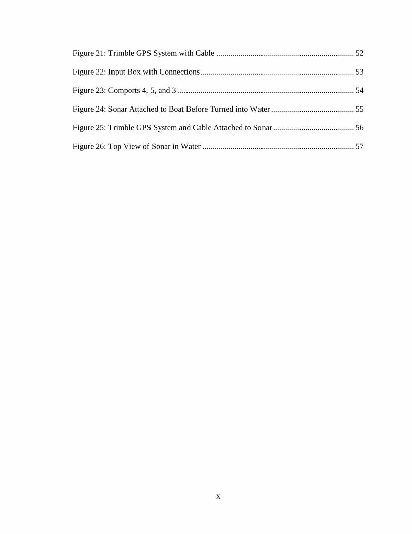
Abstract
QAUNTITATIVE ESTIMATE OF MASS SEDIMENT
MOVEMENT WITH SONAR IN DEER CREEK RESERVOIR
Ashley Nichole Childers
Department of Civil and Environmental Engineering
Master of Science
Sediment movement within a reservoir affects various reservoir processes and can
influence water quality. Quantifying this movement is a key element when evaluating the life
and quality of a reservoir. Sediment movement may be determined and quantified by many
methods. This study explores the ability to quantify and monitor sediment mass movement in
Deer Creek Reservoir (DCR) using SONAR. Sonar uses sound waves to detect distance to and
from specified objects. To monitor DCR I used sonar to measure bottom elevations and GPS to
accurately locate each measurement. I selected seven cross sections at the inflow of DCR and
surveyed them with SONAR multiple times over 63 days. Each time I surveyed a line, I covered
the line twice – once in each directions. From the surveys I was able to document changes in the
sediment surface showing both deposition and erosion. I found that the sediment moved along
the channels during the survey period. Each cross section gave new information and trends
relating to sediment movement and how these changes were related to the drawdown of the
water. The cross sections showed both deposition and erosion depending on the distance from
the reservoir head, which changed over the survey period.


Acknowledgements
I would like to thank my advisor, Dr. Gustavious P. Williams, for working with me
throughout my project. I would also like to thank the Department of Civil Engineering for
purchasing and allowing me to access our new sonar equipment. Additionally, I am thankful for
the funds provided through the U.S. Bureau of Reclamation for work on this project. I would
also like to thank the members of the Deer Creek Research group for all their help with the boat
and set up of the survey equipment. Finally, I would like to thank my family for their support in
the completion of this project.


vii
Table of Contents
Abstract .......................................................................................................................................... iv
Acknowledgements ......................................................................................................................... v
Table of Contents .......................................................................................................................... vii
Table of Figures ............................................................................................................................. ix
List of Tables ................................................................................................................................. xi
1. Introduction ............................................................................................................................... 13
2. Study Area ................................................................................................................................ 17
3. Methods..................................................................................................................................... 21
3.1 Sonar Equipment .................................................................................................. 21
3.2 Set up ...................................................................................................................... 23
3.3 Study Plan .............................................................................................................. 24
4. Processing ................................................................................................................................. 27
5. Objectives ................................................................................................................................. 29
6. Results ....................................................................................................................................... 31
6.1 Line 1 Data and Discussion .................................................................................. 33
6.2 Line 2 Data and Discussion .................................................................................. 34
6.3 Line 3 Data and Discussion .................................................................................. 35

viii
6.4 Line 4 Data and Discussion .................................................................................. 36
6.5 Line 5 Data and Discussion .................................................................................. 38
6.6 Line 6 Data and Discussion .................................................................................. 39
6.7 Line 7 Data and Discussion .................................................................................. 40
6.8 Sonar Images – Example ...................................................................................... 41
7. Conclusions ............................................................................................................................... 43
References ..................................................................................................................................... 45
A1 Appendix A Survey Locations and Lines .............................................................................. 47
A1.1 Mark Location .................................................................................................... 47
A1.2 Creating Planned Lines...................................................................................... 47
B1 Appendix B Equipment and Software ..................................................................................... 49
B1.1 Instructions for starting HYPACK 2009 .......................................................... 49
B 1.2 Connecting Sonar on boat ................................................................................. 51
B 1.3 To Begin Survey ................................................................................................. 58
B 1.4 Processing ........................................................................................................... 58
B 1.5 Locations............................................................................................................. 61

ix
Table of Figures
Figure 1: Deer Creek Reservoir (BOR 2009) ................................................................... 17
Figure 2: Deer Creek Tributaries (PSOMAS 2002) ......................................................... 18
Figure 3: Channel cross section using Odem eChart ........................................................ 21
Figure 4: Planed Survey Lines and Starting Points .......................................................... 22
Figure 5: Plan View of the Profile Lines for DCR ........................................................... 23
Figure 6: Sharp Slopes of Channels When Water Elevation was Low ............................. 31
Figure 7: Channel with More Rounded Edges .................................................................. 31
Figure 8: Line 1 profile. .................................................................................................... 33
Figure 9: Line 2 profile. .................................................................................................... 34
Figure 10: Line 3 profile. .................................................................................................. 35
Figure 11: Line 4 ............................................................................................................... 36
Figure 12: Section 1 of Line 4 .......................................................................................... 37
Figure 13: Line 5 profile. .................................................................................................. 38
Figure 14: Section 1 of Line 4 .......................................................................................... 38
Figure 15: Line 6 ............................................................................................................... 39
Figure 16: Line 7 profile. .................................................................................................. 40
Figure 17: eChart soundings ............................................................................................. 41
Figure 18: Hypack USB .................................................................................................... 49
Figure 19: Echotrac CVM Case and Computer Inside ..................................................... 51
Figure 20: Ethernet Cord, Socket Card, Power Cord........................................................ 52
x
Figure 21: Trimble GPS System with Cable .................................................................... 52
Figure 22: Input Box with Connections ............................................................................ 53
Figure 23: Comports 4, 5, and 3 ....................................................................................... 54
Figure 24: Sonar Attached to Boat Before Turned into Water ......................................... 55
Figure 25: Trimble GPS System and Cable Attached to Sonar ........................................ 56
Figure 26: Top View of Sonar in Water ........................................................................... 57

xi
List of Tables
Table 1: Distances of 7 Profile lines for DCR .................................................................. 24
Table 2: Survey Schedule to DCR .................................................................................... 30

xii
13
1. Introduction
The level of nutrients and pollutants in a reservoir has a profound effect on water quality
(Linnik and Zubenko 2000; Sakai, Murase et al. 2002). Deposited sediments have been identified
as a potential internal nutrient source and can provide nutrients to the reservoir water column
even when external sources are minimized. Studies were conducted in reservoirs which reduced
external inputs of nutrients, and in some areas this reduction had limited effect on eutrophication
(Gran´eli 1988; Mayer 1999). Excessive amounts of nutrients may increase productivity in
ecosystems, leading to problems with water quality (Casbeer 2009) . In addition to nutrients, the
bottom sediments of water bodies can also accumulate pollutants. The remobilization of these
substances are important mechanisms that control pollutant concentrations in aquatic
environments (Linnik and Zubenko 2000). Understanding and quantifying sediment processes in
reservoirs will allow researchers to adequately maintain a sustainable source of water (Casbeer
2009). One of the main processes is sediment movement, or resuspension.
Resuspension is a mechanical process that allows deposited sediments to become
suspended within the water column. Some of the well-recognized internal and external sources
for resuspension include wind, wave action, climate change, cold currents entering the reservoir
from rivers or groundwater, and generation or regeneration in the water body. Disturbances by
animals such as bottom-feeding fish (Lamarra 1975) and chironomid larvae (Gallepp 1979) may
also trigger resuspension. The suspended sediment have a profound effect on aquatic ecosystems
(Newcombe and MacDonald 1991). Resuspension can introduce trapped nutrients into the water

14
column, promoting the growth of algae and other aquatic organisms, adversely affecting water
quality (Anderson, Dracup et al. 1976; Gallepp 1979; Casbeer 2009).
There have been many studies on sediment movement and the effect it has on water
quality (Anderson, Dracup et al. 1976; Tarela and Menendez 1999; Linnik and Zubenko 2000;
Casbeer 2009). These studies document various methods to monitor and quantify sediment
movement. One method is to model, or conceptualize the sediment using a sediment budget. A
sediment budget is a quantitative inventory of all the sediment inputs, outputs and storage within
a defined system. The volume entering and exiting a particular section of a water body is
monitored by determining and evaluating the sediment fluxes; the sources and sinks from
different processes that give rise to additions and subtractions within a control volume.
Another approach uses the numerical solution with the finite element method to predict
reservoir sedimentation based on parabolized and laterally integrated forms of the governing
equations (Tarela and Menendez 1999). This approach is used in many computer models and
calculations to predict sediment movement. This not only allows the calculation of the
sedimentation rate, but also allows the prediction of the time evolution of bottom deposit
structures, which is fundamental when analyzing the fate of pollutants (Tarela and Menendez
1999). Mass sediment movement monitoring is another method used to develop models of
sediment mobilization, transport, and deposition. The use of Digital Elevation Models (DEM’s)
recorded by a laser scanner and the use of rare earth element oxides as tracers have both been
proven as methods to trace mass sediment movement as well (Polyakov and Nearing 2004).
DEM’s are used for measuring the movement outside of water bodies, while the use of rare earth
element oxides can trace sediment movement both in and out of the water.

15
The goal of this project is to use sound navigation and ranging (sonar) to determine the
mass sediment movement in Deer Creek reservoir. This approach is similar to developing
DEM’s with a laser scanner (Polyakov and Nearing 2004) but incorporated under water. Sonar
has generally been used as a tool for marine geology, but in recent years, mainly through the
interest in sedimentological problems of lakes and reservoirs, the use of sonar technology has
been explored in bodies of fresh water (Robert W. Duck 1987). Sonar uses sound reflection to
detect objects on the bottom surface (HYPACK). The basic principles on which sonar relies is
that the sound moves at a steady rate through a given medium, water in this case, and reflects off
objects in its path. In practice sound velocity is changed by the temperature profile, which can be
taken into account. By recording these echoes and measuring the time required for the echo to
travel from the sound source to the receiving point, calculations can determine the distance to an
object with reasonable accuracy. In some cases, sonar can be used to distinguish different
sediment depositional environments; characterizing soft sediment layers from hard packed
sediments (HYPACK ; Robert W. Duck 1987). This is useful for reservoir studies, since soft
sediments are more prone to resuspension. This study of DCR, however, did not try to
differentiate between the hard and soft sediments.
Sonar studies have been undertaken previously in fresh water reservoirs, but not for the
use of monitoring sediment movement. The most common use is for bathymetry profiles. Sonar
has been used to detect mines on the ocean floor (Blondel 2000), monitor fish in shallow
channels (Pedersen and Trevorrow 1999), create bathymetry profiles, and aid in dredging
projects. A group at the University of Illinois conducted a study using a multibeam echo
sounding to examine both the form and flow above a series of sand dunes in the Mississippi and

16
Missouri rivers (Best, Kostaschuk et al. 2001). We intend to show that sonar can be used to
monitor and quantify short term, on the order of months, sediment mass movement in reservoirs.
17
2. Study Area
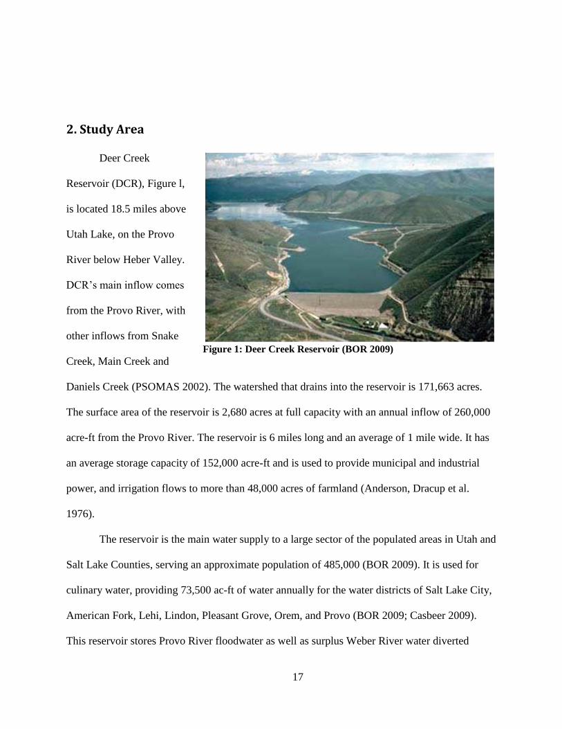
Deer Creek
Reservoir (DCR), Figure l,
is located 18.5 miles above
Utah Lake, on the Provo
River below Heber Valley.
DCR’s main inflow comes
from the Provo River, with
other inflows from Snake
Creek, Main Creek and
Daniels Creek (PSOMAS 2002). The watershed that drains into the reservoir is 171,663 acres.
The surface area of the reservoir is 2,680 acres at full capacity with an annual inflow of 260,000
acre-ft from the Provo River. The reservoir is 6 miles long and an average of 1 mile wide. It has
an average storage capacity of 152,000 acre-ft and is used to provide municipal and industrial
power, and irrigation flows to more than 48,000 acres of farmland (Anderson, Dracup et al.
1976).
The reservoir is the main water supply to a large sector of the populated areas in Utah and
Salt Lake Counties, serving an approximate population of 485,000 (BOR 2009). It is used for
culinary water, providing 73,500 ac-ft of water annually for the water districts of Salt Lake City,
American Fork, Lehi, Lindon, Pleasant Grove, Orem, and Provo (BOR 2009; Casbeer 2009).
This reservoir stores Provo River floodwater as well as surplus Weber River water diverted
Figure 1: Deer Creek Reservoir (BOR 2009)
18
through the Weber-Provo Canal and water from the Duchesne River. The reservoir releases
water for the Metropolitan Water District of Salt Lake City that flows 42 miles through an
aqueduct to Salt Lake City (Anderson, Dracup et al. 1976). The state beneficial use
classifications for the reservoir include: culinary water, recreational bathing (swimming), boating
and similar recreation (excluding swimming), cold water game fish and organisms in their food
chain, and agricultural uses (BOR 2009).
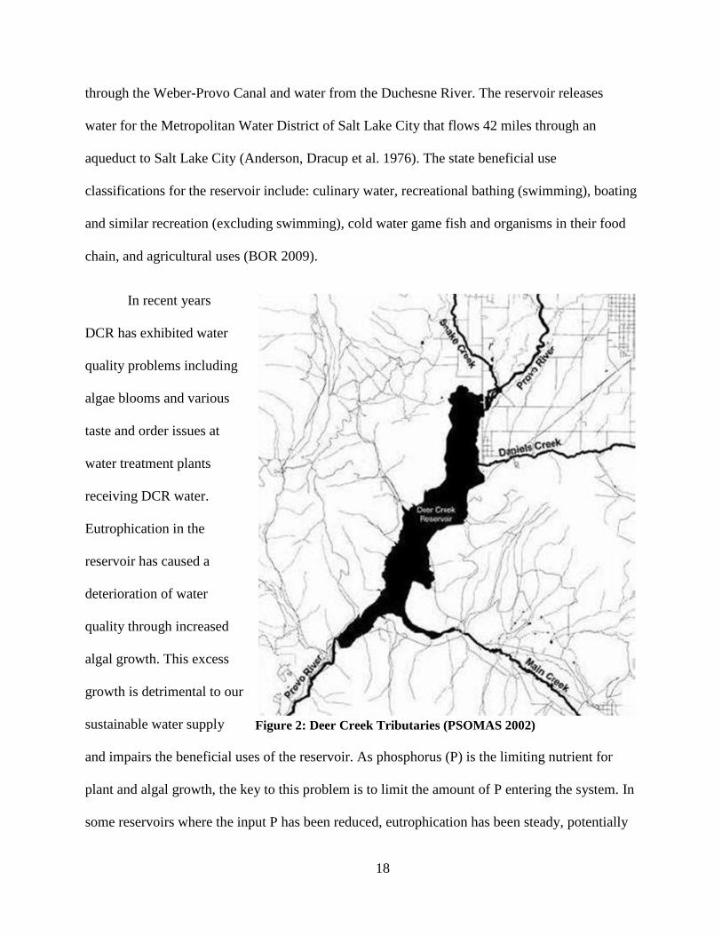
In recent years
DCR has exhibited water
quality problems including
algae blooms and various
taste and order issues at
water treatment plants
receiving DCR water.
Eutrophication in the
reservoir has caused a
deterioration of water
quality through increased
algal growth. This excess
growth is detrimental to our
sustainable water supply
and impairs the beneficial uses of the reservoir. As phosphorus (P) is the limiting nutrient for
plant and algal growth, the key to this problem is to limit the amount of P entering the system. In
some reservoirs where the input P has been reduced, eutrophication has been steady, potentially
Figure 2: Deer Creek Tributaries (PSOMAS 2002)

19
due to availability of nutrients from deposited sediments. This is referred to as nutrient recycling,
where nutrients previously trapped within the sediment become available through resuspension.
DCR has greatly improved water quality after reduction of external P loading; however,
there are still large algal blooms at times as well as other water quality issues without clear
attributable causes. One hypothesis is that sediment movement and resuspension plays a role in
these problems, providing nutrients to the water column from the sediments. To help understand
this problem I developed a method to monitor and quantify sediment movement in DCR with the
use of sonar. The first step to quantifying the amount of nutrients released to the water column is
to quantify sediment movements and resuspension.

20
21
3. Methods
3.1 Sonar Equipment
The sonar equipment I used for this research was a Single Beam Echotrac CVM Sounder.
I also used the Hypack 2009 software along with Odem eChart to perform data reduction and
analysis. Both programs are used for data collection and processing. Hypack 2009 allows you to
devise a survey plan and log points, while the eChart displays real-time high and low frequency
waves while you survey. Instructions on how to connect the sonar in the boat and begin a survey
using these programs is located in the appendix.
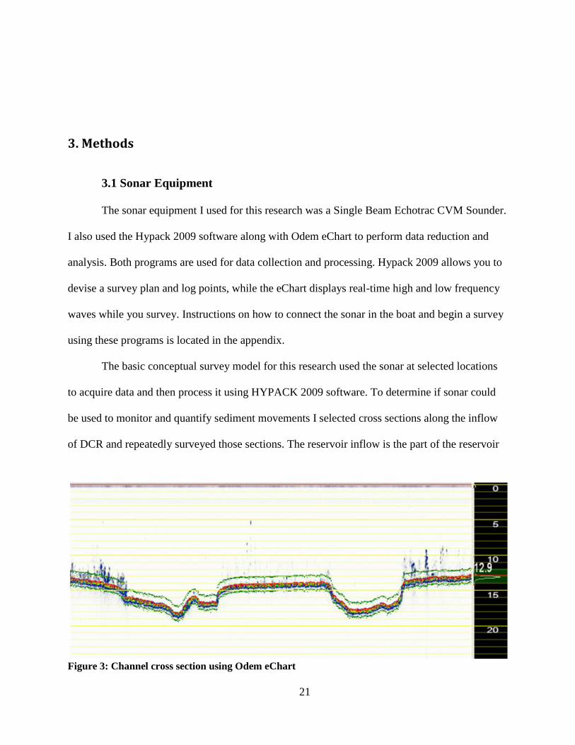
The basic conceptual survey model for this research used the sonar at selected locations
to acquire data and then process it using HYPACK 2009 software. To determine if sonar could
be used to monitor and quantify sediment movements I selected cross sections along the inflow
of DCR and repeatedly surveyed those sections. The reservoir inflow is the part of the reservoir
Figure 3: Channel cross section using Odem eChart
22
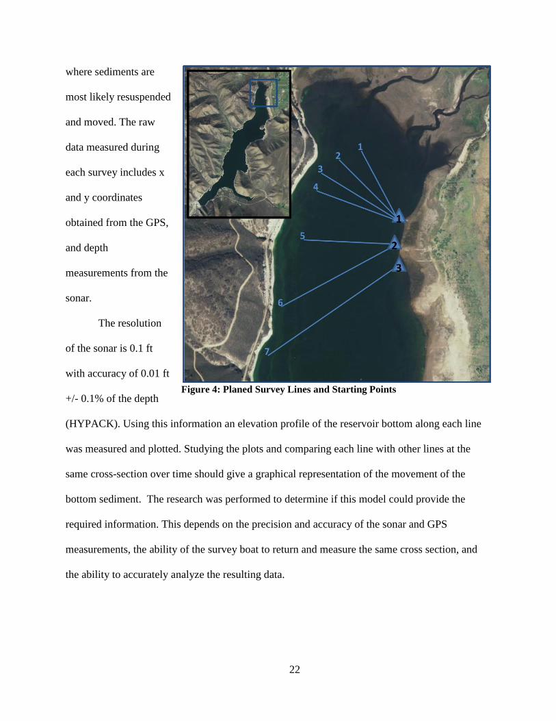
where sediments are
most likely resuspended
and moved. The raw
data measured during
each survey includes x
and y coordinates
obtained from the GPS,
and depth
measurements from the
sonar.
The resolution
of the sonar is 0.1 ft
with accuracy of 0.01 ft
+/- 0.1% of the depth
(HYPACK). Using this information an elevation profile of the reservoir bottom along each line
was measured and plotted. Studying the plots and comparing each line with other lines at the
same cross-section over time should give a graphical representation of the movement of the
bottom sediment. The research was performed to determine if this model could provide the
required information. This depends on the precision and accuracy of the sonar and GPS
measurements, the ability of the survey boat to return and measure the same cross section, and
the ability to accurately analyze the resulting data.
Figure 4: Planed Survey Lines and Starting Points
23
3.2 Set up
To create a plan for
DCR, I used the sonar
system to survey sections
across the entire reservoir
near the inflow to locate any
channels. This was done by
using the Odem eChart
software to monitor the
bottom profile during the survey. An example of the Odem eChart presentation is shown in
Figure 3, which show the channel locations. Once I located a channel during the survey, I used
the HYPACK 2009 software to mark these locations (see appendix). I created a map of these
markers and analyzed it to determine the course of the subsurface channels. Using this map I
could see roughly where the canals were located and the route they traced along the lake bottom.
Using the channel locations I developed from this map, I was able to choose survey cross
sections that would allow me to monitor the main channels for sediment movement. The final
cross sections were chosen in locations that would be easy to find and repeat for each survey. We
determined that even with GPS guidance during a survey, it was beneficial to have visible
landmarks on the shore to help navigation. A planned line profile was created with all the survey
cross sections (see appendix); this allowed me to return to the same profile lines each time I
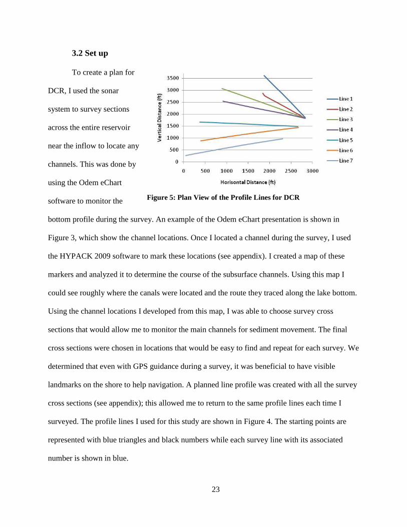
surveyed. The profile lines I used for this study are shown in Figure 4. The starting points are
represented with blue triangles and black numbers while each survey line with its associated
number is shown in blue.
Figure 5: Plan View of the Profile Lines for DCR

24
Figure 5 is a plot of the profile lines that shows their relative distances and relationships.
The top of the figure is near the inflow of DCR, while the starting point for each profile line is
near the eastern shore of DCR. Profile lines 1 through 4 began at starting point 1, profile lines 5
and 6 began from starting point 2, and profile line 7 began from starting point 3. Starting points 1
and 2 are about 415 ft apart, while starting points 2 and 3 are about 105 ft apart. Table 1 lists the
lengths of each profile line.
3.3 Study Plan
I collected data for this study along seven
profile cross sections near the main inflow of
DCR shown in Figure 4. Approximately every
two weeks I used the sonar to re-survey the
profile lines and gather a new dataset. The field
data collection consisted of seven survey lines
with three starting points as indicated in Figure 4.
These starting points were easy locations to identify and access with the boat each time we went
out, which aided the GPS positioning. In addition, each survey line had a visual reference to help
navigation along the line during data collection. An explanation of the starting points and land
marks used for each line is contained in the appendix.
The surveys began by positioning the boat on a starting point and then following our
planned line profile. Once positioned, I would start logging points and continue as the boat
moved along the survey line. I would stop logging once we reached the end of the line and turn
the boat around. I would re-start logging once the boat was positioned at the end of the line, and
the line would then be surveyed going back towards the starting point. This allowed me to collect
Table 1: Distances of 7 Profile lines for DCR

25
duplicate data so I could have more accurate readings. The recordings were saved using
HYPACK and organized by survey date and survey line.

26
27
4. Processing
I used HYPACK to edit the stored data for each line to prepare the data to be exported.
Tide and sound velocity profile corrections were not necessary for this research because those
parameters do not have significant changes within DCR. These correction factors would be
appropriate for surveying in locations such as the ocean or a deep reservoir. I chose to presort all
the data on the basis of the number of samples with an increment of one, which exported all the
measured data points. HYPACK also had options to perform various averaging or filtering on the
data before it was exported. These were not used, since I wanted to analyze all the data. The data
were exported as ascii text in .xyz files and analyzed with a series of Excel worksheets.
The survey data were imported into an Excel file where the x, y and z coordinates could
be viewed. To plot the data, the distance along each line for each measured point was calculated,
starting from the line starting point. This was done by calculating the distance between the x and
y coordinates of the measured point and the x and y coordinates of the line starting point. Once
the distance was calculated, the depth versus distance was plotted for each planned survey line.
The data showed some measurement noise, so the depth value was smoothed using a moving
window average with a width of ten. This was done by taking an average of the ten nearest
depths for each point, five on either side. This smoothed the data but retained most of the
original measurement locations, with the exception of the first and last five locations on each
line. These were a distance from the monitored channels and did not affect the results. The data
smoothing relieved some of the noise along each line within the plots. The new computed depth,
or z value, was used as the elevation for all analysis of that data set. These data were used to

28
create plots with distance along the line, measured from the line start point, on the abscissa, and
bottom elevation as the ordinate.
In addition to smoothing the data, elevations values were interpolated to standard
distances, every 0.25 feet, so the lines could be compared accurately. Having points at the same
locations on each data set allowed lines surveyed on the same day to be averaged together, lines
surveyed on difference days to be subtracted from each other showing change, and also allow
other quantitative comparison techniques to be used. As noted above, the data before
interpolation were plotted and visually analyzed. In addition, the interpolated values were also
plotted and analyzed using quantitative methods to identify changes that occurred in the channels
between the survey times. Detailed instructions on processing are located in the appendix.
29
5. Objectives
The objective of my work is to determine if sediment movement can be monitored and
quantified using sonar. I made that determination by studying the data and the various plots made
using the data and making conclusions based on the patterns and results I inferred from these
plots and data. In addition to the main objective of my work, the long term objective of the larger
study is to monitor and quantify sediment movement within DCR, while my study is designed to
determine if sonar is an appropriate technology to perform this monitoring. A short term goal,
both for my work and for the larger DCR study project, is to learn how to use the sonar
equipment and process the data. The results of my work will be first to determine if this approach
is adequate for measuring sediment movement, and second to develop methods for performing
this monitoring long-term as the study continues. A series of six survey trips, described in Table
2, were made to collect data in order to accomplish these goals. Table 2 lists the six data
collection trips, the date the trip was made, the lines surveyed, and DCR water elevation.
Elevation is an important variable since as the reservoir level lowers, more flow occurs in the
channels, and in this case, the area of the upper survey lines became so shallow that surveys
could not be accomplished.
The number of lines surveyed for each trip varies. Trip 1 was the taken to located the
channels and provide data to create the planned lines for the project. During trips 2 and 3 all
seven lines were surveyed two times, once heading down the line, and then coming back up the
line. During trip 4 only two lines were surveyed, on this trip each line was surveyed four times to

30
determine how repeatable the measurements were and to get more accurate results. Lines 1-3
were not accessible during trips 5 and 6 due to drawdown of the reservoir.
Table 2: Survey Schedule to DCR
Trip number Date Lines Surveyed Elevation of Water Surfave (ft)
1 06/30/09 Preliminary 5417.25
2 07/02/09 1, 2, 3, 4, 5, 6,7 5417.01
3 07/16/09 1, 2, 3, 4, 5, 6,7 5414.52
4 07/23/09 4, 6, 5412.53
5 08/11/09 4, 5, 6,7 5409.52
6 09/03/09 4, 5, 6,7 5407.50
31
6. Results
When I analyzed
the collected data, I
noticed a fluctuation of
sediment within the
channels over time. The
survey lines showed both
deposition and erosion at
various locations on
various lines between the
survey dates. In some
cases, the changes did not
appear to be from physical
processes, but were either
the results of data
collection errors or other
issues relating to the
analysis. Trends within the
channels for each survey
line are described in the
following sections. I offer an explanation of these trends that attempts to correlate the presented
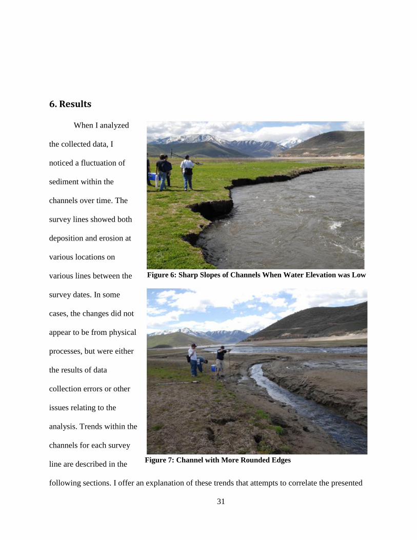
Figure 6: Sharp Slopes of Channels When Water Elevation was Low
Figure 7: Channel with More Rounded Edges

32
data with physical processes; however, these explanations may not accurately represent what is
actually happening. While enough data were collected to determine if this approach is feasible,
there were not sufficient data collected to adequately characterize all the various processes
occurring in the channels.
Lines 4 through 7 show channels with sharp slopes (see Figures 11-16) that appear to be
too steep. However, Figure 6 is an image of the upper end of DCR taken last year when the water
level was very low. This image shows sharp slopes that match the data was taken with the sonar
during my survey. Figure 7 displays a more rounded channel from the same time period, similar
to some of the channels that appear in Lines 1 – 4 (see Figures 8-11).
For most of the plots I noticed that as the distance along the survey line increases, the
data does not line up as well as it does for the beginning of the line. This appears in areas that I
did not expect any changes, which indicates that it is a problem with the measurements, rather
than actual changes in the reservoir. These data anomalies may be caused by the x and y
coordinates being converted into a distance. For each line, the starting coordinates were set as
initial points and every point taken after that is relative to those initial points. The farther a point
is from the initial location, the more potential error it can have. One potential way to mitigate
this would be rotate the coordinate system for each line so one of the ordinal directions matched
the direction of the line. Then the data would show distance from the starting point and also the
perpendicular distance of the point from the line.
33
6.1 Line 1 Data and Discussion
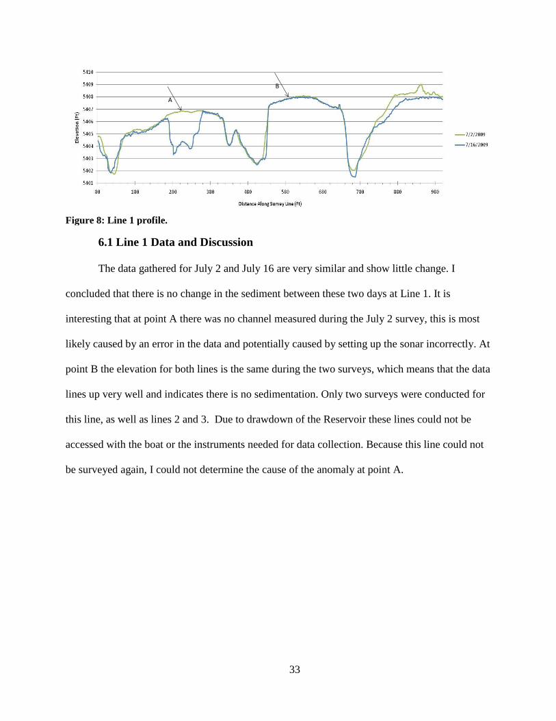
The data gathered for July 2 and July 16 are very similar and show little change. I
concluded that there is no change in the sediment between these two days at Line 1. It is
interesting that at point A there was no channel measured during the July 2 survey, this is most
likely caused by an error in the data and potentially caused by setting up the sonar incorrectly. At
point B the elevation for both lines is the same during the two surveys, which means that the data
lines up very well and indicates there is no sedimentation. Only two surveys were conducted for
this line, as well as lines 2 and 3. Due to drawdown of the Reservoir these lines could not be
accessed with the boat or the instruments needed for data collection. Because this line could not
be surveyed again, I could not determine the cause of the anomaly at point A.
Figure 8: Line 1 profile.
A
B

34
6.2 Line 2 Data and Discussion
I concluded that there is no sediment change for channels along survey line 2 between
July 2 and 16. I assumed that the elevation is incorrect and that the differences in the bottom of
the channels are relatively consistent. Point A shows the location where the errors from the
distance formula may have come into play, which also causes errors in elevation. This difference
could also be from deposition over the entire cross section, but that is unlikely. I determined that
there are not enough data to draw any conclusions of sediment movement within Line 2.
Figure 9: Line 2 profile.
A
35
6.3 Line 3 Data and Discussion
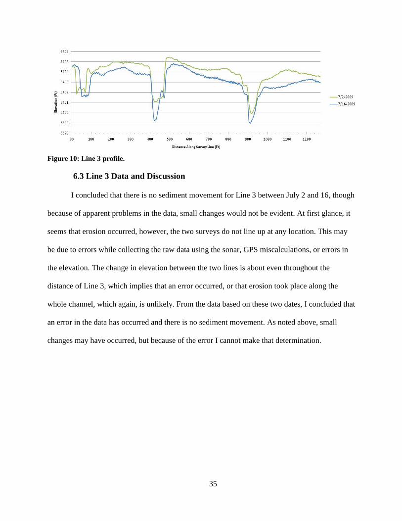
I concluded that there is no sediment movement for Line 3 between July 2 and 16, though
because of apparent problems in the data, small changes would not be evident. At first glance, it
seems that erosion occurred, however, the two surveys do not line up at any location. This may
be due to errors while collecting the raw data using the sonar, GPS miscalculations, or errors in
the elevation. The change in elevation between the two lines is about even throughout the
distance of Line 3, which implies that an error occurred, or that erosion took place along the
whole channel, which again, is unlikely. From the data based on these two dates, I concluded that
an error in the data has occurred and there is no sediment movement. As noted above, small
changes may have occurred, but because of the error I cannot make that determination.
Figure 10: Line 3 profile.
36
6.4 Line 4 Data and Discussion
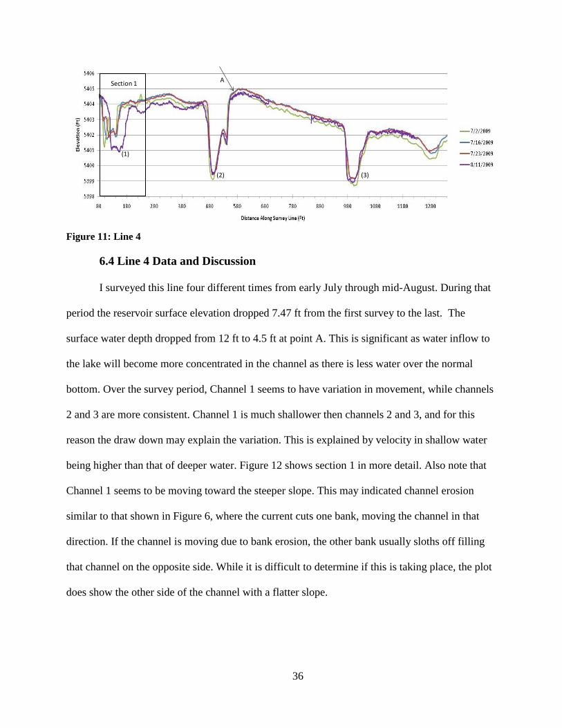
I surveyed this line four different times from early July through mid-August. During that
period the reservoir surface elevation dropped 7.47 ft from the first survey to the last. The
surface water depth dropped from 12 ft to 4.5 ft at point A. This is significant as water inflow to
the lake will become more concentrated in the channel as there is less water over the normal
bottom. Over the survey period, Channel 1 seems to have variation in movement, while channels
2 and 3 are more consistent. Channel 1 is much shallower then channels 2 and 3, and for this
reason the draw down may explain the variation. This is explained by velocity in shallow water
being higher than that of deeper water. Figure 12 shows section 1 in more detail. Also note that
Channel 1 seems to be moving toward the steeper slope. This may indicated channel erosion
similar to that shown in Figure 6, where the current cuts one bank, moving the channel in that
direction. If the channel is moving due to bank erosion, the other bank usually sloths off filling
that channel on the opposite side. While it is difficult to determine if this is taking place, the plot
does show the other side of the channel with a flatter slope.
Figure 11: Line 4
A
ASection 1
(1)
(2) (3)
37
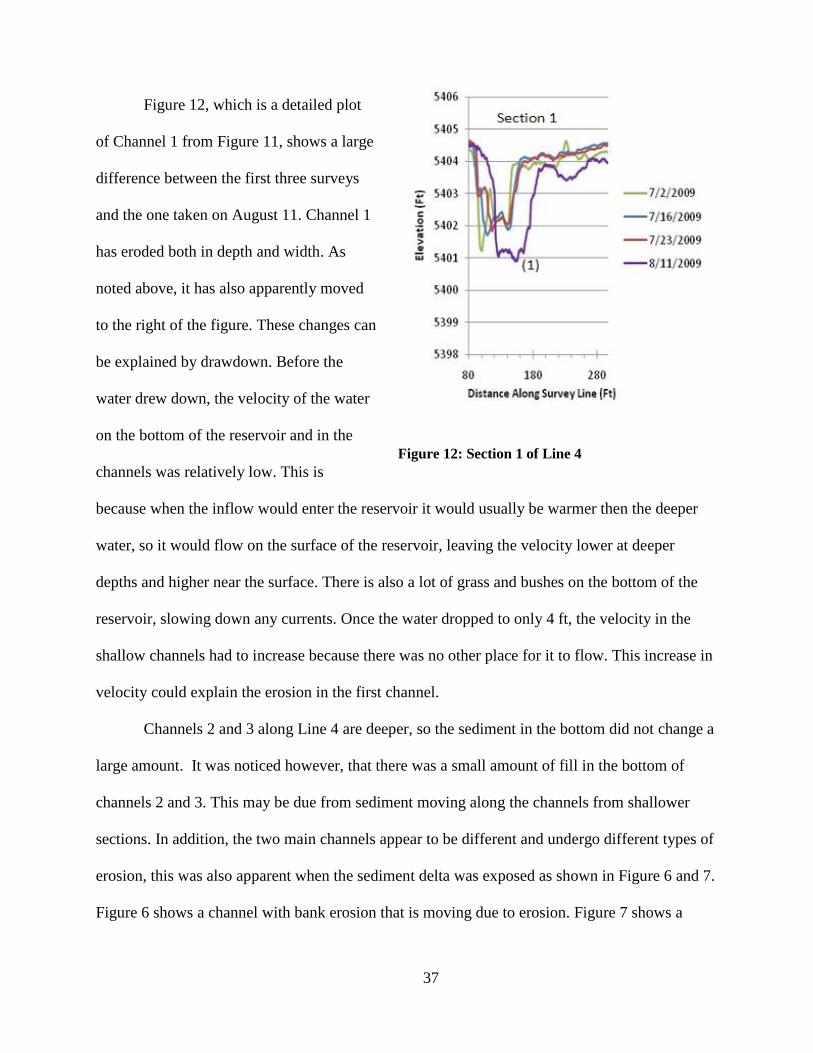
Figure 12, which is a detailed plot
of Channel 1 from Figure 11, shows a large
difference between the first three surveys
and the one taken on August 11. Channel 1
has eroded both in depth and width. As
noted above, it has also apparently moved
to the right of the figure. These changes can
be explained by drawdown. Before the
water drew down, the velocity of the water
on the bottom of the reservoir and in the
channels was relatively low. This is
because when the inflow would enter the reservoir it would usually be warmer then the deeper
water, so it would flow on the surface of the reservoir, leaving the velocity lower at deeper
depths and higher near the surface. There is also a lot of grass and bushes on the bottom of the
reservoir, slowing down any currents. Once the water dropped to only 4 ft, the velocity in the
shallow channels had to increase because there was no other place for it to flow. This increase in
velocity could explain the erosion in the first channel.
Channels 2 and 3 along Line 4 are deeper, so the sediment in the bottom did not change a
large amount. It was noticed however, that there was a small amount of fill in the bottom of
channels 2 and 3. This may be due from sediment moving along the channels from shallower
sections. In addition, the two main channels appear to be different and undergo different types of
erosion, this was also apparent when the sediment delta was exposed as shown in Figure 6 and 7.
Figure 6 shows a channel with bank erosion that is moving due to erosion. Figure 7 shows a
Figure 12: Section 1 of Line 4
38
channel with sediment bed transport. The survey lines show that Channel 1 appears to be similar
to Figure 6 and Channels 2 and 3 are more similar to Figure 7.
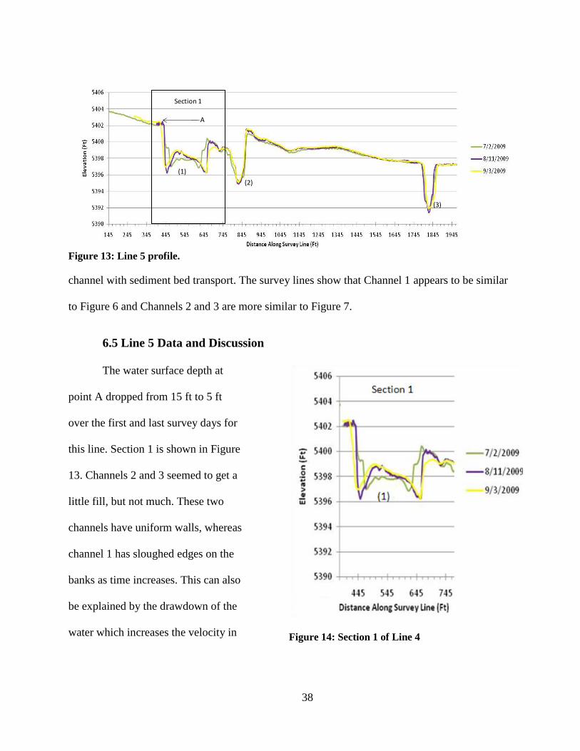
6.5 Line 5 Data and Discussion
The water surface depth at
point A dropped from 15 ft to 5 ft
over the first and last survey days for
this line. Section 1 is shown in Figure
13. Channels 2 and 3 seemed to get a
little fill, but not much. These two
channels have uniform walls, whereas
channel 1 has sloughed edges on the
banks as time increases. This can also
be explained by the drawdown of the
water which increases the velocity in
Figure 13: Line 5 profile.
Figure 14: Section 1 of Line 4
A
A
Section 1
(1)
(2)
(3)
A
39
the shallower channels as described above in section 6.4. I conclude that there is sediment
movement in channel 1 within cross section 5, due to drawdown of the reservoir.
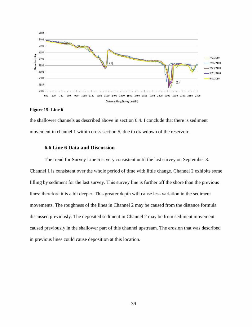
6.6 Line 6 Data and Discussion
The trend for Survey Line 6 is very consistent until the last survey on September 3.
Channel 1 is consistent over the whole period of time with little change. Channel 2 exhibits some
filling by sediment for the last survey. This survey line is further off the shore than the previous
lines; therefore it is a bit deeper. This greater depth will cause less variation in the sediment
movements. The roughness of the lines in Channel 2 may be caused from the distance formula
discussed previously. The deposited sediment in Channel 2 may be from sediment movement
caused previously in the shallower part of this channel upstream. The erosion that was described
in previous lines could cause deposition at this location.
Figure 15: Line 6
(1)
(2)
40
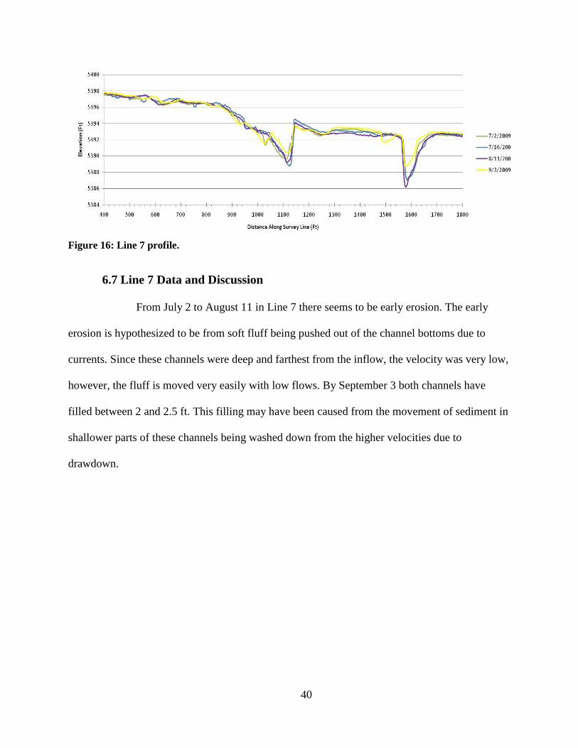
6.7 Line 7 Data and Discussion
From July 2 to August 11 in Line 7 there seems to be early erosion. The early
erosion is hypothesized to be from soft fluff being pushed out of the channel bottoms due to
currents. Since these channels were deep and farthest from the inflow, the velocity was very low,
however, the fluff is moved very easily with low flows. By September 3 both channels have
filled between 2 and 2.5 ft. This filling may have been caused from the movement of sediment in
shallower parts of these channels being washed down from the higher velocities due to
drawdown.
Figure 16: Line 7 profile.
41
A
B
C
D
E
F
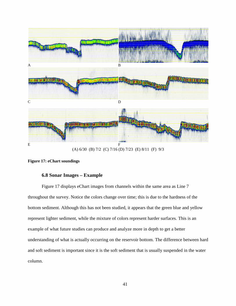
(A) 6/30 (B) 7/2 (C) 7/16 (D) 7/23 (E) 8/11 (F) 9/3
Figure 17: eChart soundings
6.8 Sonar Images – Example
Figure 17 displays eChart images from channels within the same area as Line 7
throughout the survey. Notice the colors change over time; this is due to the hardness of the
bottom sediment. Although this has not been studied, it appears that the green blue and yellow
represent lighter sediment, while the mixture of colors represent harder surfaces. This is an
example of what future studies can produce and analyze more in depth to get a better
understanding of what is actually occurring on the reservoir bottom. The difference between hard
and soft sediment is important since it is the soft sediment that is usually suspended in the water
column.

42

43
7. Conclusions
I concluded that sediment movement in DCR can be monitored and quantified using
sonar measurements and monitoring. From the surveys I was able to document changes in the
sediment surface showing both deposition and erosion that followed expected physical patterns. I
found that the sediment moved in the channels during the survey period and was adequately seen
with sonar detection. Both the short and long term goals for this project were accomplished. I
was able to learn how to successfully use the sonar to gather data and use multiple programs to
process the data. Using this data, I found that the sonar was a useful tool to use to quantify
sediment mass movement. Although this project did not develop a sediment budget, these
methods can be followed for future studies for its development.
In future studies, cross-sections closer together are suggested to get a better idea of how
each channel is connected to the next. Also each cross section should be surveyed two times
every time; once up the line, and then back down. I found that it is better to have too much data
than not enough. This will also allow you to obtain data from each accessible line every time,
which will provide more data to better estimate sediment movement along each channel. For
more accuracy, GPS differential corrections should be considered along with a different
approach to calculate the distance, such as the polar method. Also, features in HYPACK for
processing and displaying data should be analyzed in more detail. The program offers many
useful tools which were not used for this project. Those tools may reduce the need of some of the
spreadsheets used in this research. I also suggest that if the Excel spreadsheets are used for future
studies, that they be animated and linked together to save time.

44
45
References
Anderson, D. R., J. A. Dracup, et al. (1976). "Water Quality Modeling of Deep Reservoirs."
Journal (Water Pollution Control Federation) 48(1): 134-146.
Best, J., R. Kostaschuk, et al. (2001). "Quantitative visualization of flow fields associated with
alluvial sand dunes: results from the laboratory and field using ultrasonic and acoustic
Doppler anemometry." Journal of Visualization 4(4): 373-381.
Blondel (2000). "Automatic mine detection by textural analysis of COTS sidescan sonar
imagery."
BOR. (2009). "Deer Creek Dam." Retrieved June, 2009, from
http://www.usbr.gov/dataweb/html/provoriver.html.
BOR. (2009). "Deer Creek Reservoir." from
http://www.waterquality.utah.gov/watersheds/lakes/DEERCREK. pdf.
Casbeer, W. C. (2009). Phosphorus Fractionation and Distirbution across Delta of Deer Creek
Reservoir. Civil and Environmental Engineering. Provo, UT, Brigham Young University.
Master of Science: 110.
Gallepp, G. W. (1979). "Chironomid influence on phosphorus release in sediment-water
microcosms." Ecology.
Gran´eli, W. S., D. (1988). "Influences of aquatic macrophytes on phosphorus cycling in lakes."
Hydrobiologia.
HYPACK Hydrographic Survey Software User Manual. Middletown, CT.
Lamarra, V. A. (1975). "Digestive activities of carp as a major contributor to the nutrient loading
of lakes." Verhandlungen der internationale Vereinigung f¨ur theoretische and
angewandte Limnologie.
Linnik, P. M. and I. B. Zubenko (2000). "Role of bottom sediments in the secondary pollution of
aquatic environments by heavy-metal compounds." Lakes & Reservoirs: Research &
Management 5: 11-21.
Mayer, T., Ptacek, C., & Zanini, L. (1999). "Sediments as source of nutrients to hypereutrophic
marshes of Point Pelee, Ont. Canada." Wat. Res.

46
Newcombe, C. P. and D. D. MacDonald (1991). "Effects of Suspended Sediments on Aquatic
Ecosystems." North American Journal of Fisheries Management 11(1): 72-82.
Pedersen, B. and M. V. Trevorrow (1999). "Continuous monitoring of fish in a shallow channel
using a fixed horizontal sonar." The Journal of the Acoustical Society of America 105(6):
3126-3135.
Polyakov, V. O. and M. A. Nearing (2004). "Rare earth element oxides for tracing sediment
movement." CATENA 55(3): 255-276.
PSOMAS. (2002). "Deer Creek Reservoir Drainage, TMDL Study." Retrieved June, 2009.
Robert W. Duck, J. M. (1987). "Sidescan sonar applications in limnoarchaeology."
Geoarchaeology 2(3): 223-230.
Sakai, Y., J. Murase, et al. (2002). Resuspension of bottom sediment by an internal wave in Lake
Biwa. Lakes & Reservoirs: Research & Management, Blackwell Publishing Limited. 7:
339-344.
Tarela, P. A. and A. N. Menendez (1999). "A model to predict reservoir sedimentation." Lakes &
Reservoirs: Research & Management 4: 121-133.

47
A1 Appendix A Survey Locations and Lines
A1.1 Mark Location
- As you are surveying you can mark a location button to create a point on the survey
window. You can right click to edit the location where you can add information relating
to the point. These points are layer that you can turn on and off. You can also delete the
points by right clicking on them and choosing delete.
A1.2 Creating Planned Lines
- Planned survey lines are used to define where you want your vessel to go. A planned line
file contains the grid coordinates and names for each planned line in your survey area.
- For this project the planned lines were created using the cursor method.
- To do this you must first have your project open with the background file already loaded
(see appendix section B1.1).
- Open the line editor by selecting the ‘preparation’, then ‘editors’, then ‘line editor’. Or
just click on the editor icon.
- Click on image of the cursor and draw the first planned line by clicking on the starting
point, and then clicking again on the ending point.
- Open the line editor by clicking on [line editor] on the bottom left. You can review the
points of your first line, and then create a new line by selecting add line.
- You can also name the lines here if desired by selecting ‘line’, then ‘line name’ and
typing in the dialog box that appears.

48
49
B1 Appendix B Equipment and Software
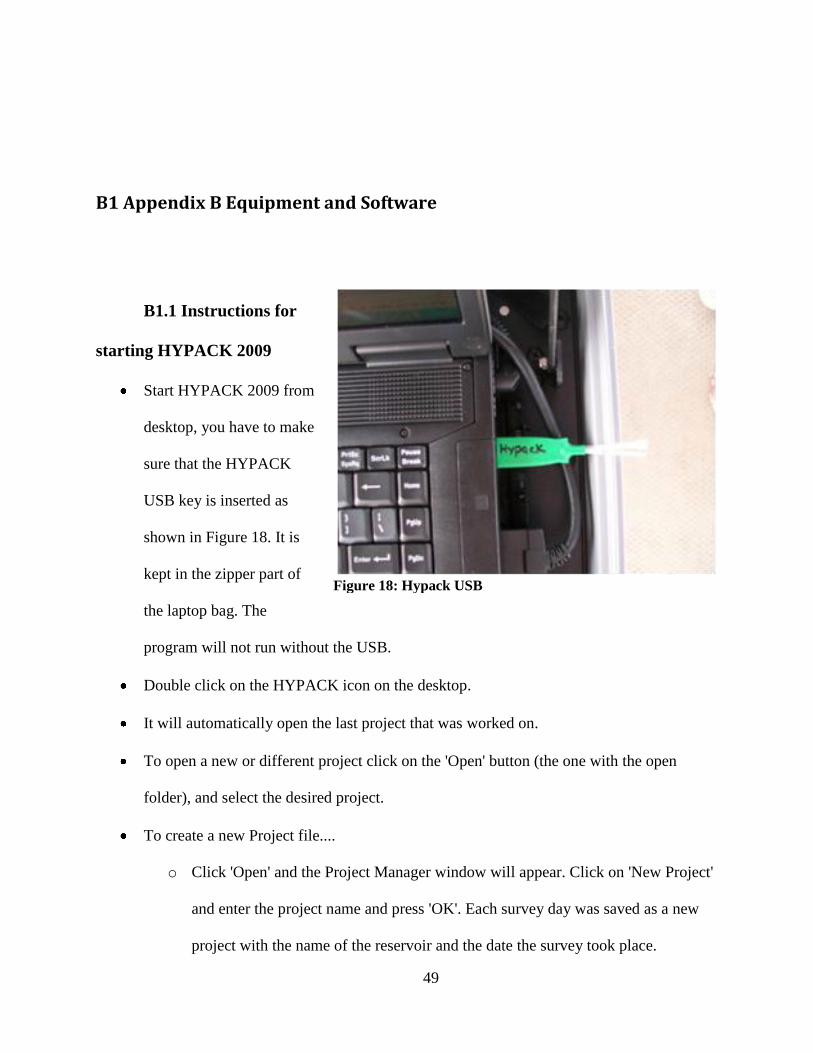
B1.1 Instructions for
starting HYPACK 2009
Start HYPACK 2009 from
desktop, you have to make
sure that the HYPACK
USB key is inserted as
shown in Figure 18. It is
kept in the zipper part of
the laptop bag. The
program will not run without the USB.
Double click on the HYPACK icon on the desktop.
It will automatically open the last project that was worked on.
To open a new or different project click on the 'Open' button (the one with the open
folder), and select the desired project.
To create a new Project file....
o Click 'Open' and the Project Manager window will appear. Click on 'New Project'
and enter the project name and press 'OK'. Each survey day was saved as a new
project with the name of the reservoir and the date the survey took place.
Figure 18: Hypack USB
50
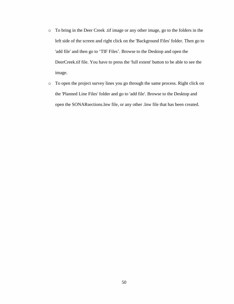
o To bring in the Deer Creek .tif image or any other image, go to the folders in the
left side of the screen and right click on the 'Background Files' folder. Then go to
'add file' and then go to ‘TIF Files’. Browse to the Desktop and open the
DeerCreek.tif file. You have to press the 'full extent' button to be able to see the
image.
o To open the project survey lines you go through the same process. Right click on
the 'Planned Line Files' folder and go to 'add file'. Browse to the Desktop and
open the SONARsections.lnw file, or any other .lnw file that has been created.

51
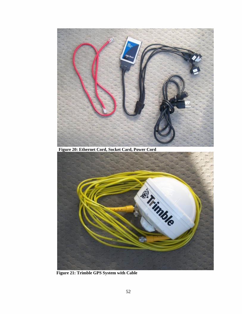
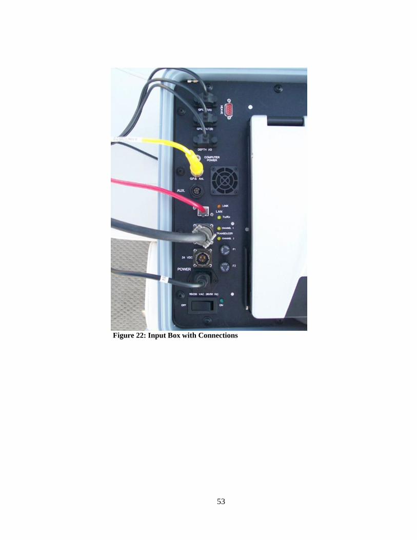
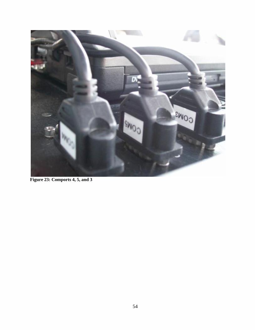
B 1.2 Connecting Sonar on boat
Connection checklist: All points must
be connected in order for sonar the work.
Figures 19 – 23 show images of the computer
and the cords.
Socket card into laptop connected
to comports 4, 5, 3 going down.
Comp4-GPS(I/0)A. Comp5-
GPS(out)B. Comp3-depth. Comp
6 should be free. Shown in Figure
23. Make sure that the socket card
is put in the lap top right side up.
If problems occur, this is a good
thing to check.
Connect the Ethernet cable to the laptop and the box where is says 'LAN'
Power cord into socket connected to the pox where it says 'POWER'
SONAR cable from sonar to box where it says 'TRANSDUCER', it screws in and
then snaps into place.
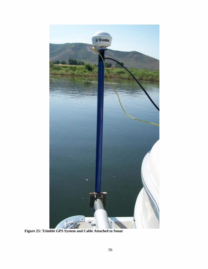
Yellow Trimble cord connected from GPS into box where is says 'G.P.S. Ant’. Make
sure the GPS is connected to the top of the Sonar bar. It just screws in on top of the
bar.
Plug in the laptop with its power cord into the socket.
Figure 19: Echotrac CVM Case and Computer
Inside
52
Figure 20: Ethernet Cord, Socket Card, Power Cord
Figure 21: Trimble GPS System with Cable
53
Figure 22: Input Box with Connections
54
Figure 23: Comports 4, 5, and 3
55
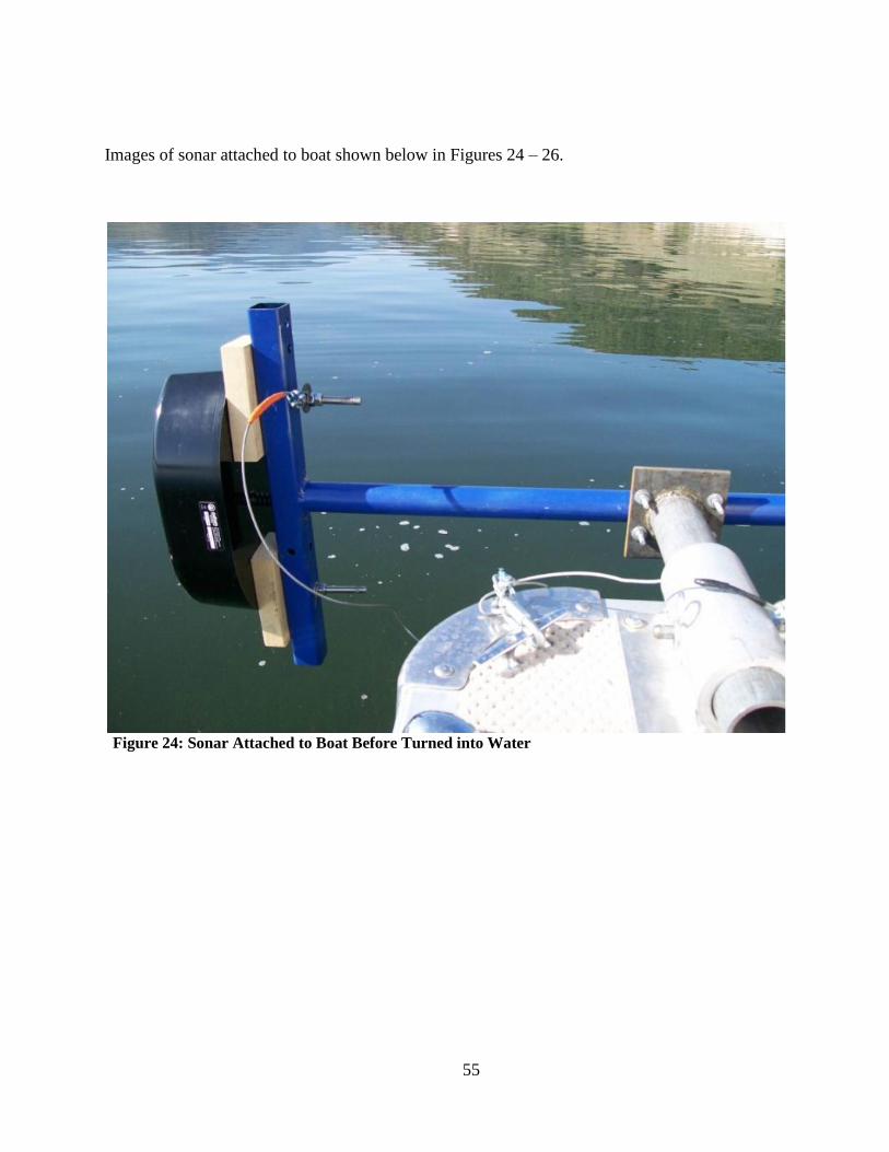
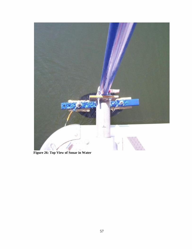
Images of sonar attached to boat shown below in Figures 24 – 26.
Figure 24: Sonar Attached to Boat Before Turned into Water
56
Figure 25: Trimble GPS System and Cable Attached to Sonar
57
Figure 26: Top View of Sonar in Water
58
B 1.3 To Begin Survey
Turn on the power switch in the box
In the Hypack window go to 'Survey' and click on 'Survey' (Make sure that the sonar
is in the water before you do this!!), otherwise you will hear a beeping alarm sound.
The image should show up and you should see where the boat is located.
Next, go to the Desktop and open eChart.exe. Go to ‘file’ and ‘connect to sounder’, or
just press the connect button. You should see two channels with markings being made
in them. The right is low frequency, and the left is high frequency.
When you are in position to begin logging points, go to the survey window and go to
‘logging’ and ‘start logging’, or press the logging button. When you are at the end of
your line press stop logging.
Also in the eChart window you want to press ‘record’ when you are logging over the
lines, and then press ‘stop recording’ when you are finished with your line.
Then turn the boat around and repeat logging and recording along the same line going
back.
B 1.4 Processing
Editing
When the data is saved it creates a .LOG file which contains .RAW data files. These
.RAW data files are made up of all the logging points taken for each line separately.
In order to export any of the data, you must have .EDT files. To get these files you
have to edit your .RAW data files.
Open HYPACK and open the project you are working with.
Make sure that there are .RAW files there under the ‘Raw Data’ folder.

59
In the top menu bar go to ‘Processing’ then ‘Single Beam Editor’.
Go to ‘File’ then ‘Open’ and select the .LOG file that is in your project folder, it will
automatically be there for you to select.
Once you select the .LOG file the ‘Catalog’ box will appear. This allows you to pick
one line at a time or you can just select them all at one time. For my research I would
just press ‘select all’ so I could edit every line at the same time. If you want a more
detailed picture to see in the editor you can do one at a time.
Once you select the line or lines you want to work with, the ‘Corrections’ window
will appear. If you have tide or sound velocity corrections you can open the files from
here, but we are not working with any corrections for this research. You can choose
which depth to use, for my project I just used depth 1.
Then the ‘Read Parameters’ window appears and nothing should be changed. In the
‘presort tab’, ‘yes, all data’ should be selected and the Basis should be in ‘Number of
Samples’ with an Increment of ‘1’. This can be changed if you want different
increments of data; however, these are the settings I used. Also, the Selection should
be on ‘Average Depth’.
It will then read in the data you selected.
You can read in the Manuel about processing options for this step if there is anything
significant you want to do. I did not change anything else for my research.
Save the data and now you have .EDT files to work with.
Exporting
Go to ‘Final Products’ in the menu bar and go to ‘Export’.
60
In the ‘Export’ window, right click on the .LOG file under the ‘Edited Data Files’
folder and press on ‘Enabled’. You can do this for all the .EDT files or just certain
ones you want. I found it is easier to do one at a time.
Under the Output File section under Format, make sure that the ‘Soundings (XYZ)’ is
selected. Under Name, click on the folder on the right. In the ‘Save As’ window write
the name of the XYZ file you want to create and press ‘Save’.
Then press ‘Convert’ and this makes a XYZ file.
If you convert all the lines at the same time, when you open the .xyz file there is just
one long list of values. If you do this, in order to tell where each line starts and stops,
there will be an x,y, and z heading at the beginning of each line. You have to make
sure you know what order the lines are in, this is just selecting them in the HYPACK
window and knowing what planned line they were on.
Otherwise just export one line at a time and you will not run into any problems.
Excel Worksheets
First open a new Excel file where you will open the .xyz files.
Then cut and paste in the x, y and z values in to the Excel file named ‘DClines’ under
the Line1Raw tab. Another column is created called Distance. Under the 1 tab there
will be Distance, Z smooth, and Elevation columns. The Distance is the same but the
Z smooth is the average of ten of the raw z values to get a smoother line.
Next you will copy out the Distance and Elevation columns and paste them into the
Excel file named ‘INTERPOLATION_DC (version 1)’ into the Raw-X and Raw-Y
columns. Fill out a start and end x value (this will be the area in which will be

61
interpolated over) and a delta (which is the increment value). I used .25. Then press
Fill NEW-X button, and then the INTERPOLATE button.
Once this is done, open the Excel file named ‘DCInterpolated’ and paste in the new X
and Y values. For multiple surveys over the same line for the same day, the average
will be taken. This is the line in which will be graphed to represent that survey line.
B 1.5 Locations
The table below is a list of the locations and land marks used for this Deer Creek study.
Some of the land marks are ones in which may be hard to find, so I suggest having the planned
lines turned on while trying to find these locations and pick new land marks that will be easier
for you to follow which are along the planned lines for future research.
Line Number Starting Point Location Land Mark Description
1
1
In tree area where there is a
little clear area for boat
Left edge of barn on the
opposite side of the water
2 1 Bushes just left of the
pavilion on opposite shore
3 1 Straight down from the
telephone pole
4 1 Left side of dirt area by the
waters edge
5
2
In front of the house just West
of the launch ramp
Towards rocky point
6 2 Brown spot near red dirt
streak near water’s edge
7
3
Little bush in the water by
white house
Big red spot of dirt

62