Quantifying the Spatial Issues in Human Dimensions Research

Deirdre M. Mageean1, Raymond J. O’Connor2, Suzanne Cashman Rain3, and N. Scott Urquhart4

1 Department of Resource Economics and Policy, University of Maine, Orono, ME04469-5703

2 Department of Wildlife Ecology, University of Maine, Orono, ME 04469-5755

3 VP Database Marketing Analytics, KeyBank, Cleveland, OH 44114

4 Department of Statistics, Colorado State University, Fort Collins, CO 80523-1877

Prepared for presentation at the Open Meeting of the Global Environmental Change Research Community, Montreal, Canada, 16-18 October, 2003

Abstract Global assessment of human-environment interactions is intrinsically hierarchical, requiring that we infer how local and regional processes will manifest themselves in regional and global conditions, respectively. But the ability to embed local intensive case studies of social and ecological processes within spatially extensive regional or global demographic and environmental data is hindered by the presence of spatial autocorrelation. Spatial autocorrelation - wherein nearby points are more alike in social and ecological characteristics than are more remote points - can create, as it were, hills and valleys of data similarity that correspond to real world, local or regional human communities and ecosystems that are very different one from another. Many conventional statistical techniques, notably multiple linear regression, fail in these circumstances. First, they require either uniform conditions across the sampling domain or require a priori knowledge of the form of the non-uniformity present. Second, the presence of spatial autocorrelation violates key assumptions made in such conventional statistical analysis. Following our earlier, prototype applications of classification and regression tree (CART) analysis to human-environment data, several members of the IHDP community have obtained promising results on applying CART analysis within their own studies. Yet CART analysis is itself vulnerable to statistical artefacts arising from spatial autocorrelation. We present here a method of extending CART analysis to address spatial autocorrelation issues in spatially extensive human-environment studies, using socioeconomic and ecological datasets for the conterminous United States as examples. We show how semivariogram functions can be incorporated into CART analysis to model the spatial dependence of the data. We show that, by combining conventional with spatially-aware CART analysis, one can determine where (geographically) spatial autocorrelation modifies one’s estimate of the strength of the link between humans and environment (or vice versa). Finally we use CART models to partition the spatial dependence of human-environment responses between 1) spatial patterning in the environmental predictor variables and 2) spatial patterning in human activity that is entirely independent of the environmental predictors. These techniques solve what has previously been acknowledged to be one of the biggest technical hurdles in modeling the human dimensions of the environment. Introduction The scope of the International Human Dimensions Program is huge, ranging from land-use and land-cover change (LUCC) through the institutional and human security aspects of global environmental change to Industrial Transformation, and with cross-cutting interests in global carbon and water cycles and global food systems. Related research can cover the conversion of tropical forests to short-lived agriculture (Cervigni 2001) through desertification (Reynolds and Stafford Smith 2002) to intensification of land use around urban peripheries (Bartlett et al. 2000). Within these studies are many conducted over significant spatial extents, in which a recurring research need is to relate a human response to some set of predictor environmental variables or vice versa. Thus remotely sensed data covering large spatial extents have been combined with information on local land use dynamics e.g., Muller and Zeller’s (2002) study in Vietnam - or with socioeconomic data e.g., Seto and Kaufmann’s (2003) modeling of the Pearl River Delta in China.

Historically human response has been linked to environmental predictors with some variant of multiple linear regression (MLR), a solution requiring one to accept a set of underlying statistical assumptions about the data e.g. Wood and Porro (2002). Many of these assumptions are well-known, involving issues of linearity, of normality of data, of homoscedasticity, and so on. However, they typically also involve some less appreciated assumptions, among them the notion that the relationships of interest are the same throughout the sample space and that there are no interactions among variables except those explicitly incorporated into the model. In much environmental research, however, analysis (statistical and otherwise) is undertaken to determine the kinds of relationships that exist in the study system and the associated lack of a priori knowledge limits the optimization of MLR models. For this reason the past two decades have seen a significant move towards the use of alternative statistical modeling techniques such as General Additive Models (GAM) and Classification and Regression Tree (CART) models, readily applied to samples innocent of spatial relationships. CART in particular, has parallels to the hierarchical organization of natural systems within which anthropogenic change is constrained (Wood and Porro 2001). Where humans and their effects are involved, however, data are pre-disposed to involve spatial relationships. Humans are social beings distributed non-randomly over the landscape and their spatial relationships almost inevitably shape the patterns of any metrics associated with their study. This has long been understood, perhaps most notably by geographers, and techniques for the incorporation of spatial relationships into regression analysis have long been known. When researchers have had to turn to CART models in the absence of prior information about the relationships to be modeled, however, techniques for the recognition and quantification of spatial patterning of the data have not been available. In the present paper we describe a procedure with which to achieve this and illustrate the analysis with some preliminary data. It is well known that the spatial distribution of people over space is shaped in part by environmental factors such as climate, elevation, proximity to the coast, and so on (Cohen and Small 1998, Small et al. 2000), with a notable concentration of people into coastal areas. Urbanization is a major class of IHDP-related research, notably within the IHDP-GCTB LUCC effort (Geist 2002). Mageean and Bartlett (1998, 1999) studied patterns of population settlement into urban and coastal concentration by use of regression tree modeling of population data from the Bureau of the Census in terms of climate and remotely sensed land cover across the conterminous United States. They found that population densities were markedly lower in areas of severe winters and were higher near the coasts. They later (Bartlett et al. 2000) showed that two distinct patterns of new settlement prevailed in the U.S. The first, which they termed alpha settlement, reflected the centripetal expansion of existing urban centers of population. The second or beta settlement reflected ‘green field’ building in areas with little or no previous settlement and this settlement was differentially concentrated into environmentally fragile areas, notably certain types of coastal or barrier island land cover and certain types of desert edge. In neither of these studies were the effects of spatial autocorrelation within the data considered, although these authors acknowledged that the relationships might reflect the spatial patterning of the predictor variables (Jones et al.1998). We use here a simplified version of the datasets used in these analyses to demonstrate how failure to consider spatial relations can yield misleading results. We confine the analysis to use of the simpler dataset because of the computational complexity of any analysis of the full dataset: even a fairly powerful Dell (Austin, TX)

PowerEdge server was able to handle directly only a 25 per cent sample of the full data, and amalgamation of multiple samples (to re-constitute the full set) required consideration of several issues strictly peripheral to the main thrust of our paper. Our focus here is on the effects of failing to account for spatial autocorrelation in a CART analysis and not on which of the conclusions of the earlier papers might need reconsideration.

Methods Our population and environmental data were mapped to a regular spatial grid, a hexagonal tessellation developed for the US Environmental Protection Agency (EPA) for use in the Environmental Monitoring and Assessment Program (EMAP) (White et al. 1992). Each hexagon was approximately 640 km2 in area, with the centroids of each hexagon approximately 27 km apart and with 12,600 hexagons covering the conterminous US. Population data for 1990 were extracted from the county-level census files of the US Bureau of Census (US Bureau of Census 1990) and cross-walked to the hexagon grid by overlaying a digital county-level boundary file onto the digital hexagon grid in a GIS (ARC/INFO 1996, ESRI Inc., Redlands, CA) and area-weighting the census variable. Our original land cover and environmental data came from Loveland et al. (1991) who used Advanced Very High Resolution Radiometry (AVHRR) meteorological satellite images to derive prototype maps of 159 classes of land cover for the conterminous US at 1.1 km2 sensor resolution. We incorporated several climate variables - annual precipitation, mean January and mean July temperatures, and annual temperature variation (seasonality) - in the form of long-term climate averages from the Historical Climate Network. The data were modeled with 1 km resolution (except that precipitation was modeled to 10 km and then re-sampled to 1 km) and were summarized within each hexagon as average, minimum and maximum values. Other variables included in the environmental data set were elevation, ownership (federal or non-federal), road density (separately for major and minor roads), and stream density. All variables were expressed as within-hexagon averages and corresponding extremes (O’Connor et al. 1996). For the present analysis only three of these variables - the extent of water and water bodies in a hexagon, the density of minor roads, and long-term average temperatures in July - appeared in our simplified analysis. Statistical modeling We used the regression tree modeling capability of the S-plus analysis language (S-plus 1995, Insightful Corporation, Seattle, WA). In a regression tree analysis (Figure 1), at each node the independent variable that best discriminated the response variable was determined and used in the tree as the splitting variable for that node. Discrimination was maximized by trying all possible splitting thresholds for all possible prediction variables and choosing the variable and threshold to maximize the differences in the response variable (maximum between-group diversity). The dataset was then split into two subsets based on this threshold value and the process was repeated independently and recursively on each increasingly-homogenous subgroup until a stopping criterion was satisfied. These trees were then ‘pruned’ back to optimal size by ten-fold cross-validation (Clark & Pregibon 1992). We tested for collinearity problems among the variables in the model by randomly perturbing each independent variable in the pruned model in turn by up to 5% and re-running the analysis to check for inclusion or omission of that variable in the perturbed tree. Variables stable in the face of such perturbation could not be

markedly collinear with any other variable in the dataset. To model the spatial autocorrelation in the data we developed a new method analogous to the “pre-whitening” of traditional regression modeling in the face of spatial issues. We fitted an empirical semivariogram to the data over a maximum range of 500 miles around the centroid of each of the 12,600 points, using the module spatial in S-Plus. We then fitted a theoretical semivariogram, finding the exponential form worked best. We used this function as the basis for modeling the spatial dependence in the data. We were unable to perform the analysis of the complete dataset on the computer available to us, this being unable to handle the required inversion of the 12,600 by 12,600 variance-covariance matrix. Instead we drew a 25 per cent (N=3127 hexagons) random sample from the data points, thereby reducing the inversion to that of a 3,127 by 3,127 matrix. In effect the spatial dependency is removed by pairing each data point in turn with each of the other points and computing (via the semivariogram function) the expected value of the response variable (population density) at a point that distance away. The difference between that expected value and the empirically observed value is then equivalent to a residual whose value is to be attributed to the effects of one or more of the independent variables at that location. These variables have themselves a correlation structure reflecting any cross-correlation among them. The pairing of all data points is what necessitates the inversion of the row-wise (case-dependent) rather than merely column-wise (variable-dependent) matrix. The end result is to yield a matrix of response and independent variables from which spatial dependency has been removed. These values were then used to compute a new regression tree from which the spatial dependencies of the original analysis should now be absent.

Results Figure 1 shows the regression tree obtained when the original data were used to provide the predictor variables. The root split is based on the density of roads in the hexagon: hexagons with more that 144 km of minor roads have an average density of 825 people per square kilometer whereas hexagons with fewer roads average only 32 people per square kilometer. This link between road density and population density is hardly surprising and is considered here only for its heuristic value in revealing the effects of spatial dependency. The high density hexagons cannot be discriminated further (in terms of the independent variables considered) but the low density hexagons show a further effect. Within the low density group, those hexagons without access to large lakes or to the coast have significantly lower population density on average (25 people per square kilometer) than have the other hexagons (mean density of 147 people per square kilometer). This group in turn divides twice on the same variable (average of long-term July temperature), forming a group of relative low density hexagons located in cool (temperature below 21.67 oC), a second group of very high density (mean 503 people per square kilometer) hexagons in warmer areas (average July temperature between 21.67 oC and 23.5 oC), and a third group of lower density (98.8 people per square kilometer) where summer temperature exceeded the 23.5 oC value. The model here differs from that for population density presented by Mageean and Bartlett by virtue of being based on sample rather than comprehensive data, resulting in it being simpler and in accounting for relatively low variance in population density (19.21 per cent). It nonetheless allows us to demonstrate the effect of spatial autocorrelation and its removal here, leaving the task of applying it to the full national dataset to a separate analysis. This is entirely the result of the artificial restrictions on choice of predictors allowed be

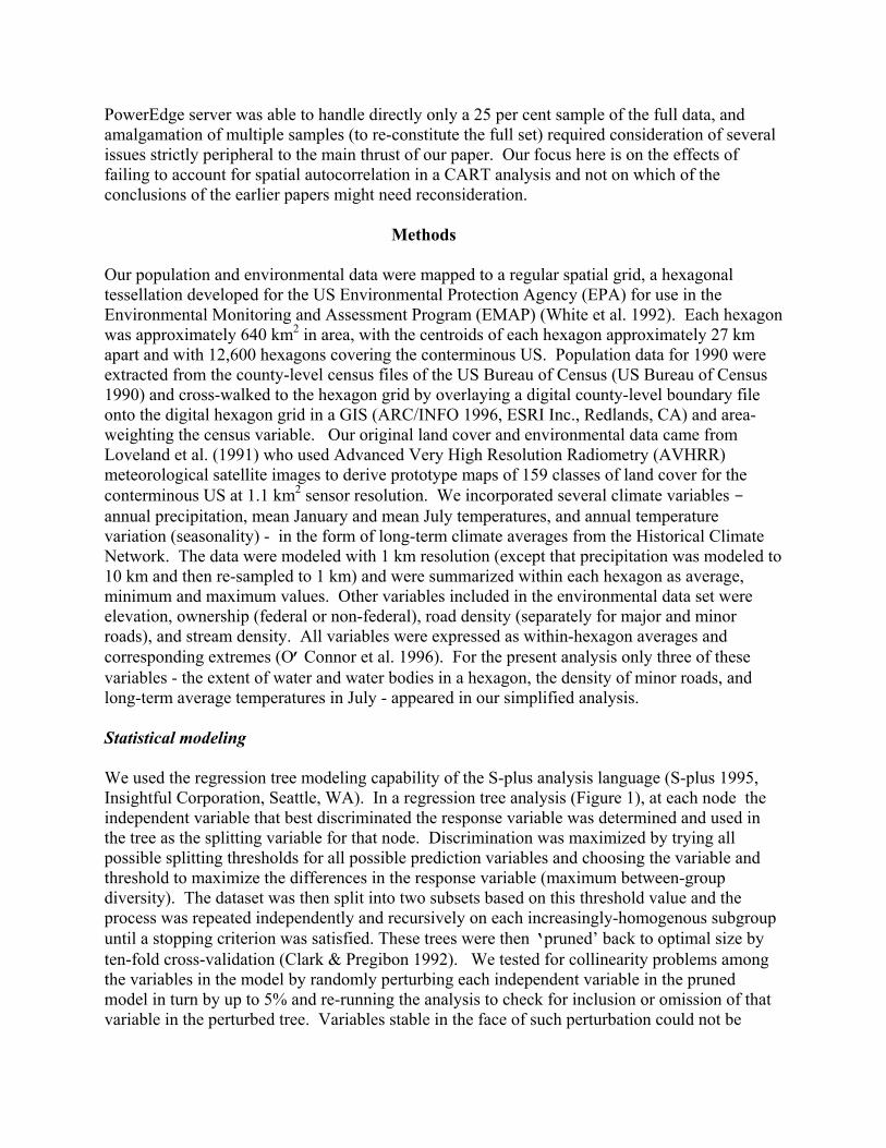
considered here in the interests of keeping the comparison simple. Figure 2 shows where these five groups of hexagons are located. The low density hexagons with little access to large water bodies (left-most node in Figure 1) form the body of the country. Among them can be seen the very high density cities associated only with high densities of roads (right-most node). Around the coast are the hexagons showing dependence on July temperatures, with the cooler sites along the Pacific coast, the northern Great Lakes, and along the New England coast. The warmer areas with high population densities are concentrated along the southern shore of Lake Michigan and Lake Erie and along the eastern coast from parts of Massachusetts south to Cape Hatteras. A few such sites also appear near San Diego and near Denver. Finally the hot areas discriminated by the regression tree extend south from Cape Hatteras around the Florida coast and along the Gulf Coast. A few such sites also appear near Denver. We thus see a fairly clear picture of climate correlates of population density being mainly coastal and of high density concentrations around roads being mainly urban. This analysis gave no consideration to any effects of spatial autocorrelation. Figure 3 (top curve) shows that there was substantial spatial dependency among points closer together than 200 miles. At larger distances the semivariance - in essence a measure of the average difference in population density between any two points that distance apart - was constant at a value of about 332 units. So neighboring points less than 200 miles apart tend to be similar to each other in population density. Note that this effect cannot be attributed to an artefact of the cross-walking of population density from county to hexagon units: there are close to four hexagons in each county (on average) which with a 17 mile centroid to centroid separation allows cross-walking smoothing over at most about 34 miles. The lower curve in Figure 3 shows the semivariogram obtained after the data had been processed to remove spatial dependency. This curve shows two points. First, because it is virtually flat, spatial dependency has been almost entirely eliminated, as desired. Second, this line is positioned at a very low value - around 3.2 units against the 332 units of the sill value of the original semivariogram - which implies that virtually all of the variance to be explained in terms of predictor variables has been removed by the adjustments for spatial dependency. This immediately implies that the regression tree analysis of the (spatially) uncorrelated data will not have much predictive power. This is confirmed by Figure 4 which presents such a tree (now based on the 25 per cent sample). Its overall accounting for the variance in population density is indeed low (9.1 per cent against the 19.6 per cent of the original regression tree). Note that it is a simpler version of Figure 1, with the climate-dependent branches of that figure deleted. Note that the threshold values for the road density effect and for the water bodies effect have both changed from the corresponding values in Figure 1. Similarly the mean population density values in the node are also different. These changes reflect the adjustment of response and predictor variables to remove the spatial effects in the initial analysis and do not have the same significance as does the disappearance of the climate effects. To help interpret the meaning of these changes, consider that all the hexagons in this sample also appeared in one or other of the nodes in Figure 1. We can therefore cross-tabulate the node memberships in Figure 4 against the same hexagons’ node memberships in Figure 1, as in Table 1. This shows, first, that the vast majority of the hexagons were not affected on removing the

spatial effects. They appeared in the leftmost node in Figure 1 and in the leftmost node in Figure 4. However, a handful of sites originally in the background group in Figure 2 now show an effect of road density that they did not display earlier: all but one moved out of the leftmost node of Figure 1 into the rightmost node of Figure 4; the remaining one moved into the middle node of Figure 4. Most of these hexagons are therefore points for which the effects of road density were previously concealed by the spatial density of the data. Similarly, Table 1 shows that the nodes indicated by Figure 1 to be sensitive to climate (summer temperatures) conditions largely appear in node 4 (low density of roads but water bodies present) in the spatially aware tree (two exceptions), indicating that the spatial autocorrelation of summer temperatures had generated misleading results. If we ignore the specifics of the different types of errors, the table shows that 92.9 per cent of the cases were correctly classified irrespective of spatial effects; 2.2 per cent (balance of leftmost column in Table 1) were incorrectly designated as being subject to environmental effects that the spatially aware analysis did not support; and 18 cases (0.6 per cent) were incorrectly lumped into the background node by virtue of their spatial autocorrelation (middle two columns, top row). Of the remaining 135 cases (4.3 per cent) 120 were incorrectly identified as having climate dependency instead of largely water body dependence and only 15 (0.5 per cent) were correctly identified as being associated with high road densities, and these effects actually accounted for less on the variance in the spatially aware than in the spatially unaware model. Figure 5 shows the locations of these four classes. Note that the errors are mixed in among the highlighted coastal and near coastal hexagons, indicating some real but weaker effect of the coast persists as a result of the water body but not summer temperature effects. Table 1. Cross-tabulation of the number (per cent)of hexagons in nodes of the spatially-aware regression tree (Figure 4) (columns) against those in the nodes of the spatially unaware regression tree (Figure 1) (rows). Analysis based on a 25 per cent sample of the hexagons in the conterminous United States.

Node Identifier 3 4 5 Total

3 2905 (92.9) 1 ( 0.0) 17 ( 0.5) 2923 (93.5)

5 23 ( 0.7) 53 ( 1.7) 0 ( 0.0) 76 ( 2.4)

7 8 ( 0.3) 17 ( 0.5) 0 ( 0.0) 25 ( 0.8)

8 31 ( 1.0) 48 ( 1.5) 2 ( 0.1) 81 ( 2.6)

9 7 ( 0.2) 0 ( 0.0) 15 ( 0.5) 22 ( 0.7)

Total 2974 (95.1) 119 ( 3.8) 34 ( 1.1) 3127 (100)

The distribution of variance associated with each of the variables differed between the original regression tree and the spatially uncorrelated version. All the effects originally attributed to summer temperatures (5.3 per cent of the variance) were associated with the spatial patterning of the data. Although the other variables - road density and access to large bodies of water - remained in the spatially uncorrelated model, their influence was markedly less than when location was ignored: the explanatory power of road density dropped from 12.1 per cent to 8.4 per cent and the influence of water bodies dropped from 2.3 per cent to 0.7 per cent.

Discussion Our analysis showed first that there exists strong spatial autocorrelation within the Bureau of the Census population data (Figure 3), such that any statistical relationships assessed from the data were like to be inflated. This spatial correlation was effectively removed by our analytical approach (Figure 3, bottom curve). Our method therefore provides an effective way of addressing the problem of spatial autocorrelation in regression tree analysis. It removes the influence of neighbors being alike, allowing analysis of the uncorrelated data to proceed under the assumptions required for valid regression tree analysis. To our knowledge this has not previously been achieved and the new procedure therefore makes a new analytical tool available, paralleling for regression tree analysis the pre-whitening methods previously available for multiple linear regression. Copies of the S-Plus code for the procedure are available on request from the authors. Comparison of the original and uncorrelated analyses here showed that the influence of most variables was over-estimated in the presence of spatial auto-correlation (Table 2). One should note, though, that this does not necessarily imply that the effect of, for example, July temperatures in the original model was artefactual. What it implies is that nearby points alike in July temperatures were also alike in population density, so that it is impossible to distinguish between population and July temperatures having a common spatial patterning versus their being causally correlated with each other. One can not use this dataset in support of an independent correlation of population with July temperature. In a similar manner the initial assessment of links between population density and road density and between population density and access to water bodies indicated stronger correlations than were eventually evident in the spatially uncorrelated data. For these variables, therefore, some influence on population density was manifest irrespective of location (Figure 4). (Note that this conclusion is subject to the standard caveat that correlation does not entail causation.) Additional linkage between variable and population density may also have been present but, if so, it involved a spatial patterning of variable and population density and the interpretation of this necessitates additional investigation of the data. On this point we note that the ability to map the geography of locations (hexagons) that changed status before and after the incorporation of spatial information (Figure 5) is a powerful tool. It allows investigators identify these locations and subject them to appropriate additional analysis. In the present study we did not attempt this deeper analysis, the analysis being deliberately based on a simplified data set highlighting the core issue, but in a definitive study this would be the typical next step to take. Conversely, the fact that most of the hexagons in the present analysis did not shift out of the commonest node provided considerable assurance that the conclusions reached about them were robust against spatial issues. We also note that the cross-tabulation of node memberships across the two regression trees (Table 1) was highly informative. First, it showed that most of the data points were unaffected, most of them being concentrated in the largest node of low density hexagons with low road density and no water bodies but some persisting in the minor, less populated nodes. But the cross-tabulation also showed which members of the dataset were affected in what way by the adjustment for spatial autocorrelation. Some hexagons initially apparently influenced by summer temperatures were relocated to new nodes on the basis of road density. (One should note here that these road densities were now the uncorrelated values rather than the original data

that might have been cross-correlated with summer temperatures.) These hexagons were thus identified as having different dynamics with respect to summer temperatures and road density than had those hexagons remaining in situ. In this way a new research question is raised. The approach developed here suggests a tiered sequence of response by investigators concerned about the possible influence of spatial autocorrelation on their analysis. A first step should be to determine the empirical semivariogram for their response variable. Many statistical packages contain a spatial statistics module that allows one to do this straightforwardly. If the semivariogram shows little evidence of autocorrelation, no further action is needed and conventional analysis may proceed. If, however, the plot shows substantial curvature, then investigation of the effects of autocorrelation is indicated. Where regression analysis is the goal, the procedure developed here will partition out the uncorrelated components of the dataset to yield a data set with which analysis can proceed. Subsequent mapping of locations moving or not moving between nodes will then reveal the geography of the spatial influences. Whether the effects that have “disappeared” on adjustment for spatial autocorrelation are to be treated as artefact or as a spatially patterned effect of interest to the analyst is a research question, to be determined by empirical investigation of the specifics of the study in hand. The cross-tabulation techniques offered here are one pathway to localizing and quantifying these effects in preparation for such further study. Acknowledgments We thank Tom Fish with help in the preparation of the diagrams. The development of the uncorrelate function used here was conducted with the financial support of a grant from the National Science Foundation to R. J. O’Connor and D. M. Mageean. Literature Cited Bartlett, J. G., D. M. Mageean, and R. J. O'Connor. 2000. Residential expansion as a

continental threat to U.S. coastal ecosystems. Population and Environment 21: 429-468. Cervigni, R. 2001. Biodiversity in the Balance – Land Use, National Development and Global

Welfare. Edward Elgar: Cheltenham, UK,. 271 pp. Clark, L.A. and D. Pregibon. 1992. Tree-based models. Pp.377-419 In Statistical Models in s,

Edited by J.M. Chambers and T.J. Hastie. Wadsworth & Brooks/Cole Advanced Books & Software: Pacific Grove, CA.

Cohen, J. E., and C. Small. 1998. Hypsographic demography: The distribution of human population by altitude. Proceedings of the National Academy of Sciences 95 (24): 14009-14014.

Geist, H. J. 2002. Status and Future of the IHDP-IGBP LUCC project. Report on the Annual NASA LCLUC Science Team Meeting, University of Maryland Inn and Conference Center, Adelphi, MD, November 20-22, 2002. http://lcluc.gsfc.nasa.gov/products/ScienceTeamMtg/2002/Present_GeistH2002.pdf

Jones, M. T., J. G. Bartlett, and D. M. Mageean. 1998. Visualising the hierarchical organization of a spatially-explicit socioeconomic system. Systems Research and Information Systems. 8:137-149.

Lavorel, S., M. Flanningan, E. F. Lambin, and M. Scholes. 2003. Regional vulnerability to fire -Feedbacks, nonlinearities, and interactions. Science.

Loveland, T.R., J. W. Merchant, D. J. Ohlen, and J. F. Brown. 1991. Development of a land-cover characteristics database for the conterminous U.S. Photogrammetric Engineering and Remote Sensing 57: 1453-1463.

Mageean, D.M., and J.G. Bartlett. 1998. Putting people on the map: integrating social science data with environmental data. Proceedings - Pecora 13: Human Interactions with the Environment - Perspectives from Space. Bethesda, Md: American Society of Photogrammetry and Remote Sensing. CD-ROM, 1 disk.

Mageean, D.M., and J.G. Bartlett. 1999. Humans and hexagons: using population data to address the human dimensions of environmental change. In: S. Morain (Ed.), GIS Solutions in Natural Resource Management: Balancing the Technical-Political Equation. Chapter 5. OnWord Press, Santa Fe, NM. p

Muller, D. and M. Zeller. 2002. Land use dynamics in the central highlands of Vietnam: a spatial model combining village survey data with satellite imagery interpretation. Agricultural Economics 27: 333-354.

O'Connor, R. J., M. T. Jones, D. White, C. Hunsaker, T. Loveland, B. Jones, and E. Preston. 1996. Spatial partitioning of the environmental correlates of avian biodiversity in the lower United States. Biodiversity Letters 3:97-110.

Reynolds, J., and M. Stafford Smith. (eds) (2002) Global desertification: Do humans create deserts? Dahlem Workshop Report No. 88. Dahlem University Press: Berlin, 438 pp.

Seto, K.C. and R. K. Kaufmann. 2003. Modeling the drivers of urban land use change in the Pearl River Delta, China: integrating remote sensing with socioeconomic data. Land Economics 79: 106–121.

Small, C., V. Gornitz, and J. E. Cohen. 2000. Coastal hazards and the global distribution of human population. Environmental Geosciences 7:3-12.

U.S. Bureau of Census (1990). Census of Population and Housing. Summary tape file - 3C. United States Department of Commerce.

White, D., J. Kimmerling, and W. S. Overton. 1992. Cartographic and geometric components of a global design for environmental monitoring. Cartographic and Geographic Information Systems 19: 5-22.

Wood, C., and R. Porro. 2001. Integrating the social and natural sciences in the study of land use and land cover change. The 2001 Open Meeting of the Human Dimensions of Global Environmental Change Research Community. Rio de Janeiro, Brazil. October 6-8, 2001. http://sedac.ciesin.org/openmeeting/01mtg/schedule.html

Wood, C. H., and R. Porro (Eds.). 2002. Deforestation and Land Use in the Amazon. University Press of Florida, Gainesville, FL

Figure 1. Regression tree for population density in 1990 in relation to environmental variables. Ellipses indicate mean density in internal nodes; rectangular boxes indicate density interminal or end node. Densities are expressed as persons per square kilometer. Variablenames are as follows: RdsMin kilometers of minor road in hexagon; lcc10 proportion ofhexagon covered by large water bodies; JlAvg long-term July average temperature(Centigrade)

RdsMin<144RdsMin>144

37.90

lcc10<0.245lcc10>0.245

32.32

25.16

JlAvg<21.67JlAvg>21.67

147.20

48.78

JlAvg<23.5JlAvg>23.5

217.80

603.20 98.85

825.50

Figure 2. Location of hexagons in each of the end nodes of Figure 1, and other locationssatisfying the node definitions. Nodes are numbered from the root node (top node)downwards, with leftwards priority. Thus node 3 is the leftmost end node (rectangularnode) in Figure 1 and node 9 is likewise the rightmost end node. All hexagons in a givenend node obey all the constraints along the branches of the regression tree linking theirnode to the root node. The regression tree here was built from a 25 per cent sample ofthe hexagons in the conterminous U.S. and the comprehensive coverage here wasachieved by mapping all national locations that satisfied each node’s defining criteria.

Nodes35789

Figure 3. The semivariogram of population density in 1990 (persons per square kilometer) for(top) the original dataset without any adjustment for spatial autocorrelation and (bottom)for the dataset modified to adjust for the spatial autocorrelation of adjacent hexagons. See text for further details.

Figure 4. Regression tree for population density in 1990 in relation to environmental variablesafter adjustment for the effects of spatial autocorrelation. Conventions are as for Figure1, except that the densities shown are adjusted values (in effect, the residuals about thevalues predicted from the semivariogram of Figure 3). The threshold values for thepredictor values are likewise those following adjustment of the data to reflect cross-correlation with spatial patterns.

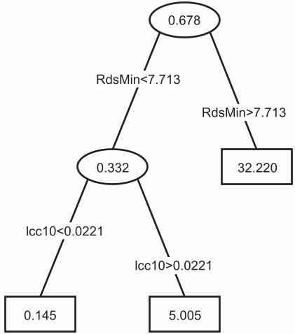
RdsMin<7.713

RdsMin>7.713

0.678

lcc10<0.0221

lcc10>0.0221

0.332

0.145 5.005

32.220

Figure 5. The distribution of the four classes of hexagons in a before and after adjustment forspatial autocorrelation classification. The map is based on a 25 per cent sample of thehexagons tesselating the conterminous U.S. and black dots indicate points not included inthe sample. Blue points were classified similarly irrespective of autocorrelation. Redpoints indicate locations where an association of high population density with highdensity of roads was concealed by spatial autocorrelation. Blue points indicate locationswhere population density was incorrectly identified as associated with summertemperature rather than with proximity to water until adjustment for spatialautocorrelation revealed the error. Yellow points indicate where population density wasassociated with proximity to water both before and after adjustment for spatialautocorrelation but more weakly so once spatial patterning was allowed for. See text formore detail.

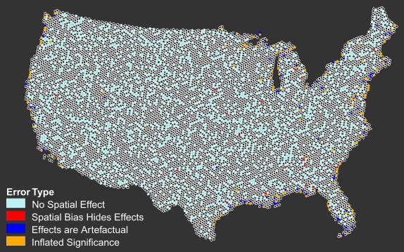
Error TypeNo Spatial EffectSpatial Bias Hides EffectsEffects are ArtefactualInflated Significance