1

photo

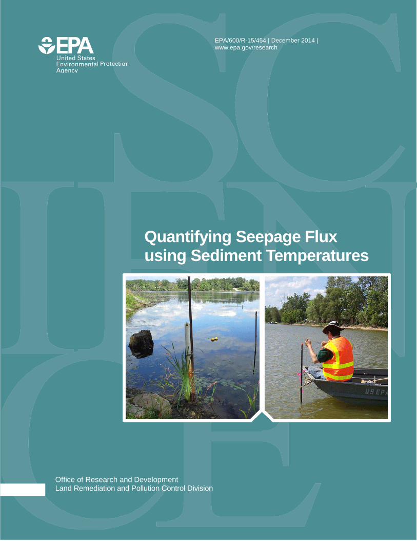
EPA/600/R-15/454 | December 2014 | www.epa.gov/research

Quantifying Seepage Flux using Sediment Temperatures

Office of Research and Development Land Remediation and Pollution Control Division

EPA/600/R-15/454 December 2014

Quantifying Seepage Flux using Sediment Temperatures

by

Bob K. Lien U.S. EPA/Nat ional Risk Management Research Laboratory/Land

Remediat ion and Pol lut ion Contro l Divis ion, Cincinnat i , OH 45268

Robert G. Ford U.S. EPA/Nat ional Risk Management Research Laboratory/Land

Remediat ion and Pol lut ion Contro l Divis ion, Cincinnat i , OH 45268

Land Remediat ion and Pol lut ion Control Divis ion Nat ional Risk Management Research Laboratory

Cincinnat i , Ohio, 45268

ii

Notice The U.S. Environmental Protection Agency, through its Office of Research and Development, funded and conducted the research described herein under an approved Quality Assurance Project Plan (Quality Assurance Identification Number L18757-RT-1-0). It has been subjected to the Agency’s peer and administrative review and has been approved for publication as an EPA document. Mention of trade names or commercial products does not constitute endorsement or recommendation for use.

iii

Abstract This report provides a demonstration of different modeling approaches that use sediment temperatures to estimate the magnitude and direction of water flux across the groundwater-surface water transition zone. Analytical models based on steady-state or transient temperature solutions are reviewed and demonstrated. Case study applications of these modeling approaches are illustrated for two different field settings with quiescent and flowing surface water systems. For the quiescent system, application of two different steady-state models to evaluate temperature records from three depths is illustrated for estimating groundwater seepage into a pond. For the flowing water system, application of two different transient models is illustrated for estimating water exchange across a granular cap placed on top of sediments in a small river. The transient models use amplitude ratio or phase shift of diurnal temperature records from two depths to estimate seepage flux. These models require isolation of a diurnal signal component from the raw temperature time-series. Two diurnal signal extraction techniques of harmonic regression and bandpass filtering were implemented and compared. The results indicate that average calculated fluxes were indistinguishable for both signal isolation techniques. However, it was demonstrated that the harmonic regression technique provided greater detail in the temporal fluctuations in calculated seepage. Application of forward modeling using 1DTempPro with the VS2DH flow and heat-transport model to assess the reliability of calculated seepage from steady-state and transient models is also demonstrated. This report covers a period from 31 July 2011 to 31 July 2012 and work was completed as of 3 August 2012.

iv

Foreword The U.S. Environmental Protection Agency (US EPA) is charged by Congress with protecting the Nation's land, air, and water resources. Under a mandate of national environmental laws, the Agency strives to formulate and implement actions leading to a compatible balance between human activities and the ability of natural systems to support and nurture life. To meet this mandate, US EPA's research program is providing data and technical support for solving environmental problems today and building a science knowledge base necessary to manage our ecological resources wisely, understand how pollutants affect our health, and prevent or reduce environmental risks in the future.

The National Risk Management Research Laboratory (NRMRL) within the Office of Research and Development (ORD) is the Agency's center for investigation of technological and management approaches for preventing and reducing risks from pollution that threaten human health and the environment. The focus of the Laboratory's research program is on methods and their cost-effectiveness for prevention and control of pollution to air, land, water, and subsurface resources; protection of water quality in public water systems; remediation of contaminated sites, sediments and groundwater; prevention and control of indoor air pollution; and restoration of ecosystems. NRMRL collaborates with both public and private sector partners to foster technologies that reduce the cost of compliance and to anticipate emerging problems. NRMRL's research provides solutions to environmental problems by: developing and promoting technologies that protect and improve the environment; advancing scientific and engineering information to support regulatory and policy decisions; and providing the technical support and information transfer to ensure implementation of environmental regulations and strategies at the national, state, and community levels. Determination of the magnitude and variability of water flow between groundwater and surface water, or seepage flux, is critical for evaluating potential impacts to the aquatic environment and for design of restoration efforts. Use of measured sediment temperatures provides a flexible and cost-effective tool to locate areas of groundwater discharge and calculate the magnitude and direction of seepage flux. Provided in this report is a review of the theoretical basis for calculating seepage flux, the requirements for design of the temperature monitoring network, and examples of data processing and calculations of seepage flux for standing and moving surface water systems. This publication has been produced as part of the Laboratory’s strategic long-term research plan. It is published and made available by US EPA’s Office of Research and Development to assist the user community and to link researchers with their clients. Cynthia Sonich-Mullin, Director National Risk Management Research Laboratory

v

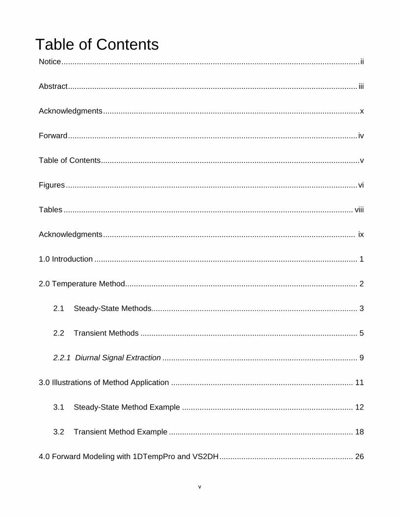
Table of Contents Notice ........................................................................................................................................ ii

Abstract .................................................................................................................................... iii

Acknowledgments ..................................................................................................................... x

Forward .................................................................................................................................... iv

Table of Contents ...................................................................................................................... v

Figures ..................................................................................................................................... vi

Tables .................................................................................................................................... viii

Acknowledgments ................................................................................................................... ix

1.0 Introduction ........................................................................................................................ 1

2.0 Temperature Method .......................................................................................................... 2

2.1 Steady-State Methods.............................................................................................. 3

2.2 Transient Methods ................................................................................................... 5

2.2.1 Diurnal Signal Extraction ......................................................................................... 9

3.0 Illustrations of Method Application ................................................................................... 11

3.1 Steady-State Method Example .............................................................................. 12

3.2 Transient Method Example .................................................................................... 18

4.0 Forward Modeling with 1DTempPro and VS2DH ............................................................. 26

vi

5.0 Summary and Research Needs ....................................................................................... 31

6.0 References ....................................................................................................................... 34

vii

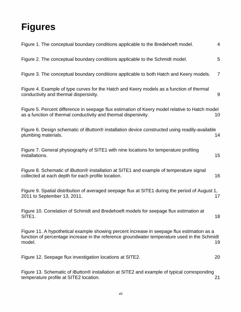
Figures Figure 1. The conceptual boundary conditions applicable to the Bredehoeft model. 4

Figure 2. The conceptual boundary conditions applicable to the Schmidt model. 5

Figure 3. The conceptual boundary conditions applicable to both Hatch and Keery models. 7

Figure 4. Example of type curves for the Hatch and Keery models as a function of thermal conductivity and thermal dispersivity. 9

Figure 5. Percent difference in seepage flux estimation of Keery model relative to Hatch model as a function of thermal conductivity and thermal dispersivity. 10

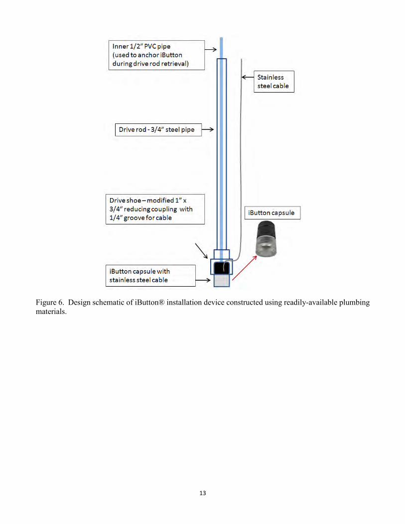
Figure 6. Design schematic of iButton® installation device constructed using readily-available plumbing materials. 14

Figure 7. General physiography of SITE1 with nine locations for temperature profiling installations. 15

Figure 8. Schematic of iButton® installation at SITE1 and example of temperature signal collected at each depth for each profile location. 16

Figure 9. Spatial distribution of averaged seepage flux at SITE1 during the period of August 1, 2011 to September 13, 2011. 17

Figure 10. Correlation of Schmidt and Bredehoeft models for seepage flux estimation at SITE1. 18

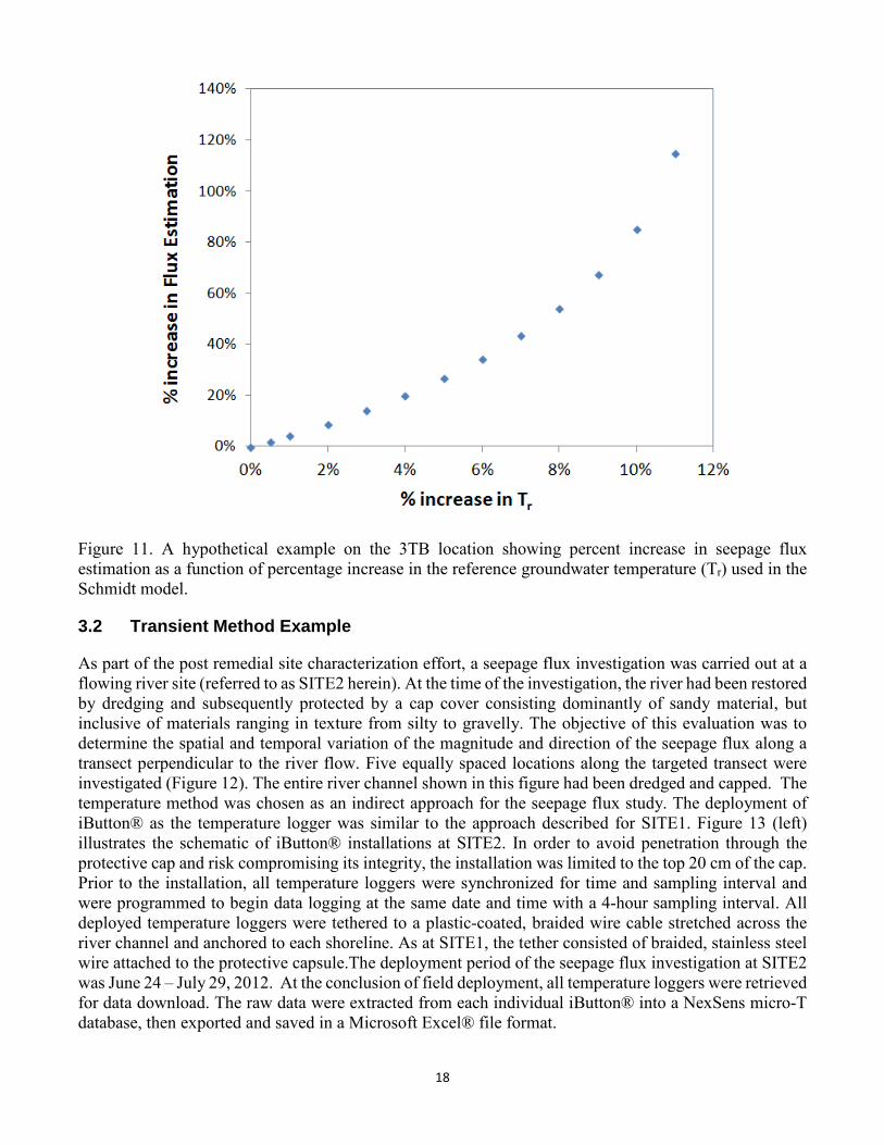
Figure 11. A hypothetical example showing percent increase in seepage flux estimation as a function of percentage increase in the reference groundwater temperature used in the Schmidt model. 19

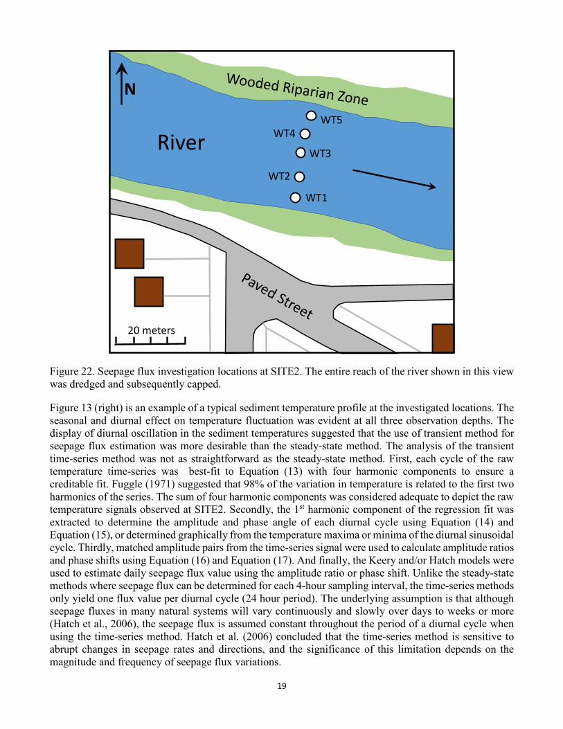
Figure 12. Seepage flux investigation locations at SITE2. 20

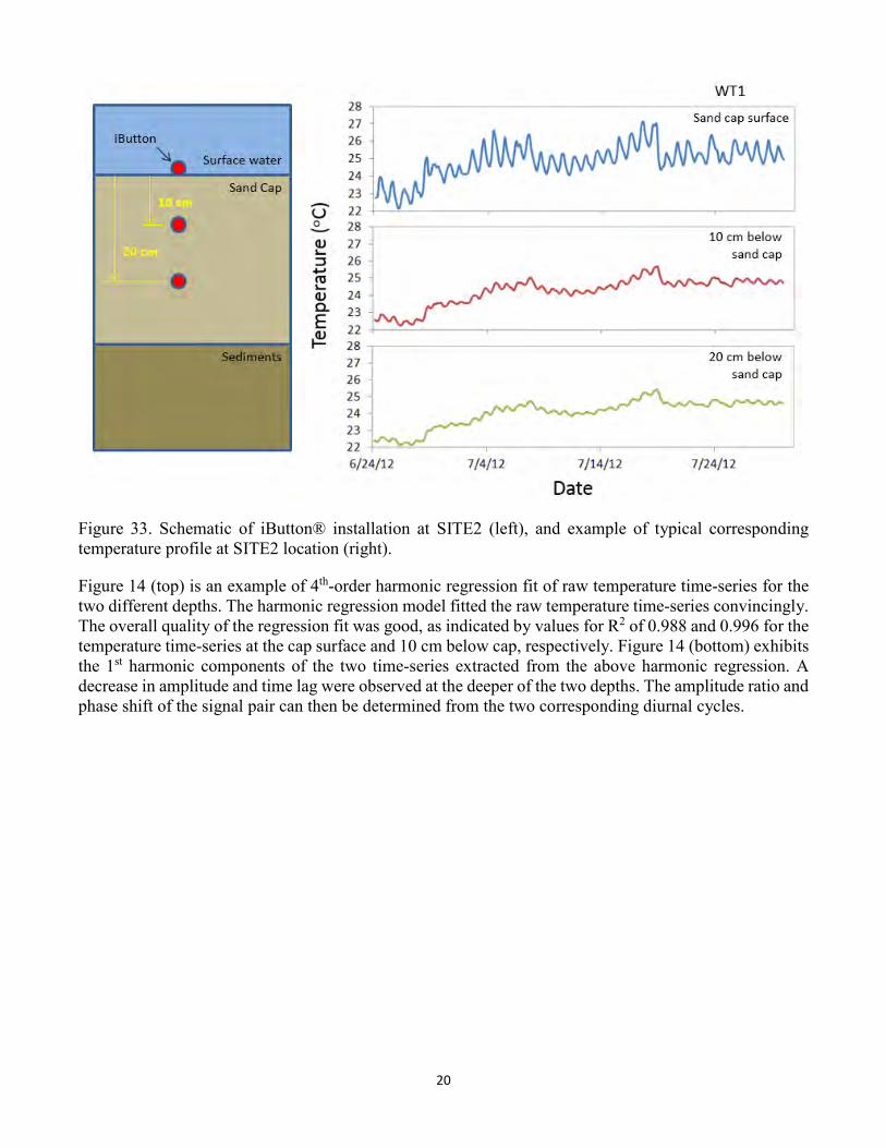
Figure 13. Schematic of iButton® installation at SITE2 and example of typical corresponding temperature profile at SITE2 location. 21

viii

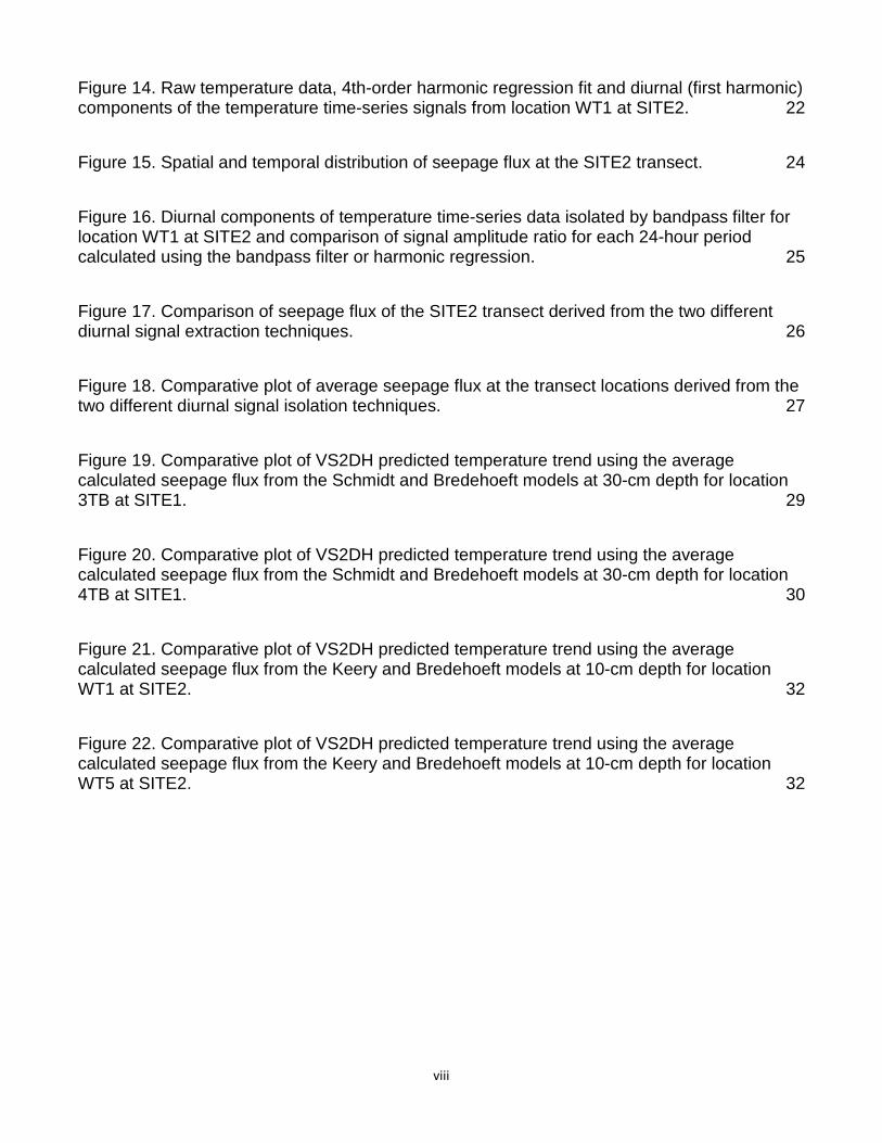
Figure 14. Raw temperature data, 4th-order harmonic regression fit and diurnal (first harmonic) components of the temperature time-series signals from location WT1 at SITE2. 22

Figure 15. Spatial and temporal distribution of seepage flux at the SITE2 transect. 24

Figure 16. Diurnal components of temperature time-series data isolated by bandpass filter for location WT1 at SITE2 and comparison of signal amplitude ratio for each 24-hour period calculated using the bandpass filter or harmonic regression. 25

Figure 17. Comparison of seepage flux of the SITE2 transect derived from the two different diurnal signal extraction techniques. 26

Figure 18. Comparative plot of average seepage flux at the transect locations derived from the two different diurnal signal isolation techniques. 27

Figure 19. Comparative plot of VS2DH predicted temperature trend using the average calculated seepage flux from the Schmidt and Bredehoeft models at 30-cm depth for location 3TB at SITE1. 29

Figure 20. Comparative plot of VS2DH predicted temperature trend using the average calculated seepage flux from the Schmidt and Bredehoeft models at 30-cm depth for location 4TB at SITE1. 30

Figure 21. Comparative plot of VS2DH predicted temperature trend using the average calculated seepage flux from the Keery and Bredehoeft models at 10-cm depth for location WT1 at SITE2. 32

Figure 22. Comparative plot of VS2DH predicted temperature trend using the average calculated seepage flux from the Keery and Bredehoeft models at 10-cm depth for location WT5 at SITE2. 32

ix

Tables Table 1. Parameters used in SITE2 seepage flux calculation ................................................... 23

Table 2. RMSE of VS2DH model prediction based on seepage flux estimated by the corresponding method .............................................................................................................. 31

x

Acknowledgments The following individuals are acknowledged for their technical reviews of an earlier draft of this report: Greg Davis (Brown and Caldwell), Donald Rosenberry (U.S. Geological Survey) and Randall Ross (U.S. EPA ORD). Patrick Clark (U.S. EPA ORD) assisted with field technical support.

1

1.0 Introduction Seepage flux is the rate of water exchange across the sediment-water interface. Hillel (1982) defined flux as the volume of water flowing through a unit cross-sectional area per unit time (L3/L2T). Equivalent to Darcy velocity, the net unit of seepage flux is length per time (L/T). Terms such as specific discharge, groundwater discharge, and groundwater seepage are commonly used interchangeably to depict seepage flux. Seepage flux is a quantity vector and is bidirectional in nature. In the following discussion, positive values of seepage flux represent upward groundwater discharge, while negative values of seepage flux represent downward groundwater recharge to the aquifer. The magnitude and direction of seepage flux is largely dependent on natural and anthropogenic processes locally and regionally (Hatch et al., 2006).

For sites where contaminant exchange across the groundwater-surface water transition zone occurs, it is important to assess the relative contribution of groundwater seepage to contaminant exposure and to consider this exposure route in the evaluation of potential risk management procedures (USEPA, 2005; USEPA, 2008). The interactions of groundwater and surface water and its importance have been thoroughly documented (Sophocleous, 2002; Winter et al., 1998). In spite of the numerous techniques available for the measurement of flow exchanges (Kalbus et al., 2006; Rosenberry and LaBaugh, 2008), quantifying seepage flux continues to be challenging. Hatch et al. (2006) described applicable spatial and temporal scales, assumptions, uncertainties, cost, and limitations of numerous methods for estimating seepage flux. Although heat-flow theory has been influential in the development of the theory of groundwater flow, interest in using temperature measurements themselves in groundwater investigations has been sporadic (Anderson, 2005). Sediment temperature is relatively easy and inexpensive to measure. With the advancements of temperature sensor technologies that enable remote and continuous measurements and improved analytical techniques and computational capabilities, the renewed interest in sediment temperature method could potentially make quantitative estimation of groundwater seepage simple and cost effective.

The purpose of this review is to provide an overview of the prevailing analytical models that have been developed to use temperature measurements to estimate seepage flux in hydrologic settings where steady-state or transient conditions may be encountered within the monitored groundwater-surface water transition zone. Using temperature data acquired from two case study locations, application of the different modeling approaches is illustrated, along with assessment of some issues concerning data acquisition, data pre-processing and model selection. The measurement and analysis methods employed in this review represent one of many options available to characterize seepage flux using sediment temperature measurements. Where appropriate, alternative approaches to data acquisition and analysis are noted by reference to examples in the peer-reviewed literature.

2

2.0 Temperature Method It has long been recognized that the flow of groundwater can affect the subsurface thermal distribution (Stallman, 1963; Suzuki, 1960). It is feasible to use heat flux as a natural tracer to characterize groundwater and surface water interactions (Anibas et al., 2011; Baskaran et al., 2009; Cartwrig, 1970; Conant, 2004; Constantz, 2008; Gamble et al., 2003; Jensen and Engesgaard, 2011; Lowry et al., 2007; Schmidt et al., 2006; Silliman and Booth, 1993). Over the years, following on the theory of interaction between heat conduction processes and advection of water, researchers have developed methods utilizing sediment temperatures to inversely quantify seepage fluxes (Bredehoeft and Papadopulos, 1965; Hatch et al., 2006; Keery et al., 2007; McCallum et al., 2012; Schmidt et al, 2007; Stallman, 1965; Suzuki, 1960). Specifically, there are four commonly used derivations of the general equation for the simultaneous, one-dimensional (1D) transport of heat and water through saturated sediments: (1) Bredehoeft model (Bredehoeft and Papadopoulos, 1965), (2) Schmidt model (Schmidt et al., 2007), (3) Hatch model (Hatch et al., 2006), and (4) Keery model (Keery et al., 2007). The Bredehoeft and Schmidt models are based on the assumption of steady-state temperature conditions, whereas the Hatch and Keery models are based on the assumption of transient-state temperature conditions. None of these inverse methods requires model calibration. The uncertainty in the flux estimation originates from the combination of uncertainties in the value of input parameters and the potential disparity between the boundary conditions imposed by the models and the actual physical conditions of the site (Shanafield et al., 2011).

The underlying theory of using sediment temperatures to quantify seepage flux evolves from the assumptions that the sediment is thermally and hydraulically homogeneous, the direction of flow is predominantly vertical within the physical boundaries of the monitored area, and that sediment temperature profiles are subjected to influences of diurnal and seasonal oscillations in the temperature of surface water. The zone of oscillation, or depth of penetration of a diurnal temperature signal into the sediment, depends largely on the magnitude and direction of the seepage flux (Conant, 2004; Schmidt et al., 2007). For upward groundwater seepage (discharge), the zone of diurnal oscillation generally decreases in depth as flux increases. But for downward seepage (recharge), the effect is reversed such that the depth of penetration of the diurnal temperature signature increases as flux increases (e.g., Stonestrom and Constantz, 2003). Below the transient zone of diurnal oscillation is the zone of quasi-steady-state conditions where temperature variation is less pronounced with increasing depth. This depth zone coincides with the zone of seasonal variation (Lapham, 1989; Stonestrom and Constantz, 2003). Seasonal temperature variations can penetrate deeper into sediments, but this occurs over a longer time frame than is typically evaluated when monitoring diurnal temperature signal propogation into sediment. Although in reality the vertical sediment temperature profile will most likely include data both influenced by transient-state and quasi-steady-state conditions, Anibas et al. (2009) suggested there will likely be periods throughout the year where transient influences on the temperature signal will be negligible such that the data can be approximated to be at quasi-steady-state. These periods exist when changes in the average air temperature are not large during the monitoring period, which occur during the maximum and minimum of sinusoidal temperature oscillations occurring during weekly, monthly or seasonal cycles.

Stallman (1963) defined the general differential equation for anisothermal flow of an incompressible fluid through isotropic, homogeneous porous medium as

(1)

3

where T = Temperature at any point at time t (oC), ρf cf = Volumetric heat capacity of the fluid (J m-3K-1), ρfscfs = Volumetric heat capacity of the saturated porous medium (J m-3K-1), kfs = Thermal conductivity of the saturated porous medium (J s-1m-1K-1), x,y,z = Distance along a Cartesian coordinates (m), qx, qy, qz, = Components of fluid velocity in the x, y, and z direction (m s-1), t = Time (s). For a one-dimensional anisothermal vertical flow system, the general equation can be simplified to (Stallman, 1965; Suzuki, 1960)

(2)

In the case of a one-dimensional steady-state flow of heat and fluid, the equation is further reduced to (Bredehoeft and Papadopulos, 1965)

(3)

2.1 Steady-State Methods

Two derivations of analytical solutions for the general heat and water transfer equation that assume adherence to steady-state conditions are considered in this report. Bredehoeft and Papadopulos (1965) solved Equation (3) for steady-state, vertical groundwater flow between two constant-temperature finite boundaries. The solution applies to both upward and downward flow. The analytical solution is given as

(4)

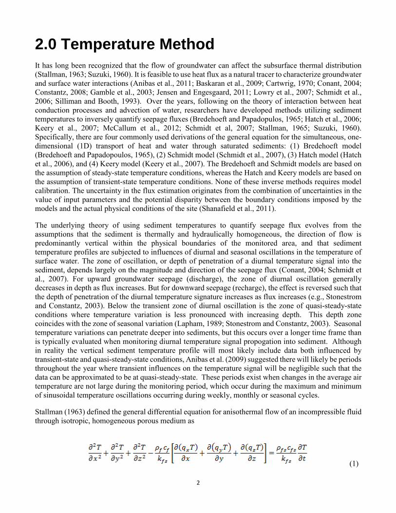
where To is the sediment temperature at the sediment surface, Tz is the sediment temperature at depth z, and TL is the sediment temperature at depth L. The conceptual boundary conditions pertinent to the Bredehoeft model are show in Figure 1. Three temperature observation points are required for this model. While the diagram in Figure 1 implies that To can only be located at the sediment surface, it could also be positioned at a depth below the surface, depending on the depth interval of interest. There are several examples in the literature that demonstrate calculated seepage flux varies as a function of depth within sediments (Briggs et al., 2012b; Cranswick et al., 2014; Jensen and Engesgaard, 2011; Vogt et al., 2010). Both the temperature profile and the seepage flux are required to be in steady-state condition. If these conditions are satisfied or can be approximated, then seepage flux can be computed using Equation (4). Because the solution is implicit, flux qz must be solved iteratively. Equation (4) presents a slight modification from the original (Bredehoeft and Papadopulos, 1965) solution so that upward flow is positive.

4

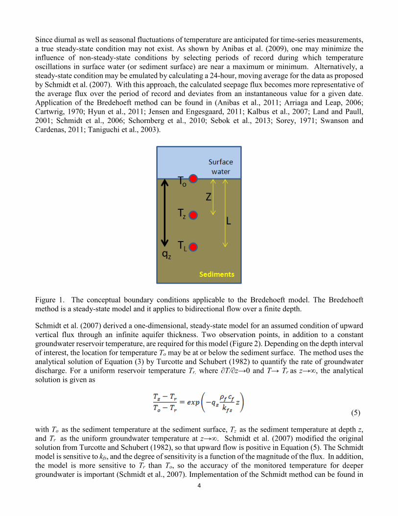
Since diurnal as well as seasonal fluctuations of temperature are anticipated for time-series measurements, a true steady-state condition may not exist. As shown by Anibas et al. (2009), one may minimize the influence of non-steady-state conditions by selecting periods of record during which temperature oscillations in surface water (or sediment surface) are near a maximum or minimum. Alternatively, a steady-state condition may be emulated by calculating a 24-hour, moving average for the data as proposed by Schmidt et al. (2007). With this approach, the calculated seepage flux becomes more representative of the average flux over the period of record and deviates from an instantaneous value for a given date. Application of the Bredehoeft method can be found in (Anibas et al., 2011; Arriaga and Leap, 2006; Cartwrig, 1970; Hyun et al., 2011; Jensen and Engesgaard, 2011; Kalbus et al., 2007; Land and Paull, 2001; Schmidt et al., 2006; Schornberg et al., 2010; Sebok et al., 2013; Sorey, 1971; Swanson and Cardenas, 2011; Taniguchi et al., 2003).

Figure 1. The conceptual boundary conditions applicable to the Bredehoeft model. The Bredehoeft method is a steady-state model and it applies to bidirectional flow over a finite depth.

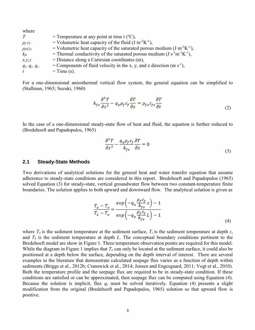
Schmidt et al. (2007) derived a one-dimensional, steady-state model for an assumed condition of upward vertical flux through an infinite aquifer thickness. Two observation points, in addition to a constant groundwater reservoir temperature, are required for this model (Figure 2). Depending on the depth interval of interest, the location for temperature To may be at or below the sediment surface. The method uses the analytical solution of Equation (3) by Turcotte and Schubert (1982) to quantify the rate of groundwater discharge. For a uniform reservoir temperature Tr, where ∂T/∂z→0 and T→ Tr as z→∞, the analytical solution is given as

(5)

with To as the sediment temperature at the sediment surface, Tz as the sediment temperature at depth z, and Tr as the uniform groundwater temperature at z→∞. Schmidt et al. (2007) modified the original solution from Turcotte and Schubert (1982), so that upward flow is positive in Equation (5). The Schmidt model is sensitive to kfs, and the degree of sensitivity is a function of the magnitude of the flux. In addition, the model is more sensitive to Tr than To, so the accuracy of the monitored temperature for deeper groundwater is important (Schmidt et al., 2007). Implementation of the Schmidt method can be found in

5

(Brookfield and Sudicky, 2013; Kikuchi et al., 2012; Swanson and Cardenas, 2011).

Figure 2. The conceptual boundary conditions applicable to the Schmidt model. The Schmidt method is a steady-state model, and it only applies to upward vertical flow through an infinite aquifer thickness.

2.2 Transient Methods

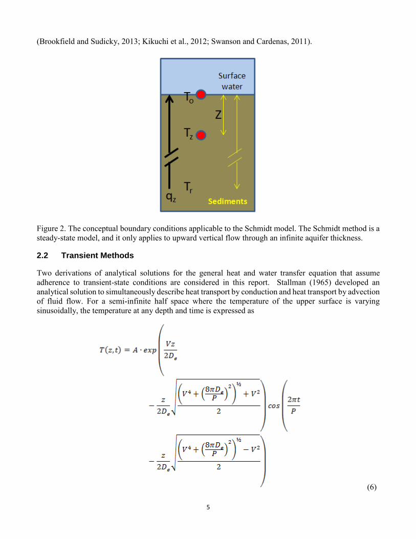
Two derivations of analytical solutions for the general heat and water transfer equation that assume adherence to transient-state conditions are considered in this report. Stallman (1965) developed an analytical solution to simultaneously describe heat transport by conduction and heat transport by advection of fluid flow. For a semi-infinite half space where the temperature of the upper surface is varying sinusoidally, the temperature at any depth and time is expressed as

(6)

6

where A is amplitude, P is period, V is thermal front velocity, De is effective thermal diffusivity, and z is depth (Goto et al., 2005; Hatch et al., 2006; Stallman, 1965). The above equation is subject to the assumptions (McCallum et al., 2012; Stallman, 1965) that (1) fluid flow is in the vertical direction only (Cuthbert and Mackay, 2013; Roshan et al., 2012), (2) fluid flow is at steady state (Anibas et al., 2009), (3) fluid and solid properties are constant in both space and time (Ferguson and Bense, 2011), and (4) fluid and solid temperatures at any particular point in space are equal at all times (Roshan et al., 2014). For each of these assumptions, the reader is referred to published evaluations (cited in parentheses) in which the impact of the various assumption violations has been examined. In general, studies comparing temperature-based methods to alternative characterization methods (direct and indirect) for determining seepage flux show that the departures from ideal conditions are quantitatively acceptable (e.g., Briggs et al., 2014; Hunt et al., 1996).

Hatch et al. (2006) solved Equation (6) for the thermal front velocity as a function of amplitude ratio Ar and phase shift ΔФ relations:

(7)

(8)

where Δz is the spacing between two observation points and De is the effective thermal diffusivity. McCallum et al. (2012) pointed out some confusion in Hatch et al. (2006) concerning the inconsistent representation of Darcy velocity and its relationship to thermal front velocity and thermal diffusivity. To set out the terms, which deviates from Hatch et al. (2006), the effective thermal diffusivity De is herein defined as a function of thermal dispersivity β and thermal front velocity V based on (de Marsily, 1986; Ferguson, 2007; Rau et al., 2012):

(9)

Since the solution of both Equation (7) and (8) is implicit, thermal front velocity V must be solved iteratively. Once V is solved, qz can be calculated by

(10)

The conceptual boundary conditions pertinent to the Hatch model are shown in Figure 3. Two temperature observation points in the diurnal oscillation zone with at least one full diurnal period are required to apply the Hatch method. The concepts of amplitude ratio and phase shift, determined from the diurnal components of the temperature time-series at two different depths, are illustrated in Figure 3. Seepage flux is estimated by solving Equation (7) or Equation (8) after amplitude ratio and phase shift are determined. McCallum et al. (2012) modified the original solution from (Hatch et al., 2006) so that upward flow is positive in Equation (7). Hatch et al. (2006) stated that temperature sensor spacing, streambed thermal parameters, and the absolute magnitude of measured temperature variations all influence

7

applicability of the method. Application of the Hatch method can be found in (Briggs et al., 2012a; Gordon et al., 2012; Hatch et al., 2010; Jensen and Engesgaard, 2011; Kikuchi et al., 2012; Lautz and Ribaudo, 2012; Lautz, 2010; Lautz, 2012; Shanafield et al., 2011; Swanson and Cardenas, 2011).

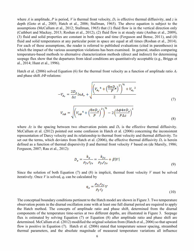
Figure 3. The conceptual boundary conditions applicable to both Hatch and Keery models (left). These methods are time-series models which apply to bidirectional flow over a finite boundary between two observation points in a zone of diurnal oscillation. The concept of amplitude ratio (Ar) and phase shift (ΔФ) of diurnal components from different depths is illustrated (right).

Similar to the concept of the Hatch method, Keery et al. (2007) rearranged the solution of Stallman (1965) to compute vertical seepage flux in terms of amplitude ratio (Ar) or the phase shift (ΔФ) of two diurnal temperature signals at different depths,

(11)

(12)

where H= ρfcf /kfs, P is the period, and Δz is the distance between the two temperature observation points. For this derivation, Keery et al. (2007) assumed that thermal dispersivity (β) exerted a minor influence on seepage flux and, thus, omitted it from the final analysis expression. The conceptual boundary conditions shown in left-hand panel of Figure 3 are also applicable to the Keery model.

Two temperature observation points in the diurnal oscillation zone with a full period of diurnal time series data are required for this model. If the monitored system satisfies the assumed conditions in deriving Equation (6), then seepage flux can be determined by Equation (11) or Equation (12). In general, only one of the roots of Equation (11) is a real number, and the other two are a conjugate complex pair. In the event that there is more than one real root, only a single real root should be accepted as the representative value. A null value should be assigned where all three roots are real numbers (Keery et al., 2007). Equation (11) presents a slight alteration from the original solution of Keery et al. (2007) so that upward flow is positive. Note that the Keery method is akin to the Hatch method. The difference between the two methods is that

8

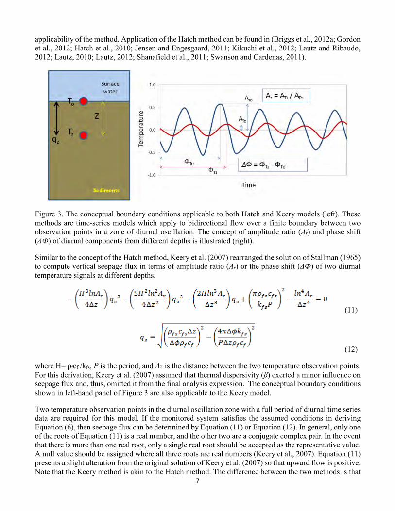
thermal dispersivity, which is often an indefinite value for the site of interest, was not included in the Keery model. Keery et al. (2007) concluded that the effect of neglecting thermal dispersivity in their analysis is insignificant. The premise by Keery et al. (2007) is not unique. Schmidt et al. (2007) set thermal dispersivity to zero in their model simulation, stating that thermal dispersion is negligible compared to thermal conduction, as suggested by Hopmans et al. (2002). Luce et al. (2013) also neglected thermal dispersivity in developing an explicit solution for the diurnal forced advection-diffusion equation, citing issues of identifiability between the effects of dispersion and diffusion observed by Anderson (2005). Figure 4 shows an example of the similarity between the Keery and Hatch solutions as the two type curves overlay when the value of thermal dispersivity is small. The type curves begin to deviate further as the value of thermal dispersivity increases. However, as suggested by Rau et al. (2012), it is apparent that the divergence induced by thermal dispersivity is insignificant in the low seepage flux range. Portions of the type curves overlay, regardless of the thermal dispersivity value, when the seepage flux is low. Eventually the seepage flux attains a value above which the influence of thermal dispersivity becomes significant and the type curves diverge.

Figure 4. Example of changes in Hatch type curves, as a function of thermal conductivity (kfs) and thermal dispersivity (β), relative to the Keery type curve where the thermal dispersivity is neglected.

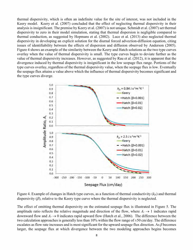
The effect of omitting thermal dispersivity on the estimated seepage flux is illustrated in Figure 5. The amplitude ratio reflects the relative magnitude and direction of the flow, where Ar → 1 indicates rapid downward flow and Ar → 0 indicates rapid upward flow (Hatch et al., 2006). The difference between the two calculation approaches is generally less than 10% within the flow range of ±50 cm/day. The difference escalates as flow rate increases and is most significant for the upward seepage flux direction. As β becomes larger, the seepage flux at which divergence between the two modeling approaches begins becomes

9

smaller and the rate of divergence increases. The result of this comparison is an indication that caution should be taken when applying the Keery method in settings where seepage flux may exceed ±50 cm/day. This theoretical analysis points to the importance of revisiting whether site conditions reasonably adhere to the assumptions underlying a particular model and consideration of using alternative model(s) that better align with site conditions. For additional perspective, the application of the Keery method can be found in (Gordon et al., 2012; Munz et al., 2011; Swanson and Cardenas, 2011).

Figure 5. Percent difference in seepage flux estimation of Keery model relative to Hatch model as a function of thermal conductivity and thermal dispersivity. The amplitude ratio Ar → 1 indicates rapid downward flow; Ar → 0 indicates rapid upward flow.

2.2.1 Diurnal Signal Extraction

Both the Hatch and Keery methods are transient models which use the amplitude ratio Ar or the phase shift ΔФ of two diurnal temperature time-series to derive seepage flux. Since the analysis is based on the assumption that the daily temperature cycle in surface water is the source of the diurnal variations, the model solution requires a full 24-hour period of sinusoidal temperature data for the analysis. The observed raw temperature signal is composed of a longer-term trend, a sinusoidal component that may consist of several harmonics, and irregular white-noise components (Gordon et al., 2012). In order to extract the diurnal sinusoidal signal from the raw temperature observations, a harmonic regression

10

model (Gordon et al., 2012; Vogt et al., 2010), similar to a Fourier series approximation, is used to best-fit each full cycle of temperature measurements using Equation (13),

(13)

where yt is the observed time-series, Tt is a trend, t is time, i is the harmonic number and a, b and ω are the respective cosine, sine coefficients and frequency. The amplitude Ai and phase angle ϕi of the respective harmonic can be calculated by (Davis, 1967)

(14)

(15)

Because the observed diurnal cycle is defined by the observed data points, it is apparent that the amplitude and phase angle of a time-series are inherently affected by the sampling interval. A practical corollary would suggest a finer sampling interval should yield better chances for adequately defining these two properties of the sinusoidal signal. As suggested later, an hourly sampling frequency is desired in order to properly define the phase shift between temperature signals.

The first harmonic, or the diurnal frequency component, of the harmonic regression is the signal of interest for the seepage flux computation. After the amplitude and phase angle of the first harmonic are determined for each observation point, the amplitude ratio Ar and the phase shift ΔФ can be calculated using Equation (16) and Equation (17), respectively (Gordon et al., 2012), or determined graphically from the temperature maxima or minima of the diurnal sinusoidal cycle. The seepage flux qz can then be solved using the Hatch or the Keery model. It is important to note that seepage flux calculated with phase shift only yields the magnitude of the flux, but not its direction.

(16)

(17)

As an alternative to harmonic regression, a bandpass filter which leaves intact the components of the data within a specific band of frequencies and eliminates all other components, can also be used to isolate the diurnal cyclical signal (Hatch et al., 2006; Hatch et al., 2010; Kikuchi et al., 2012; Munz et al., 2011; Shanafield et al., 2011; Wu et al., 2013). The bandpass filter operates by mathematically converting time-domain data into frequency-domain data. Subsequently, the diurnal component of the temperature signal is isolated by applying an inverse-transformation of the data with a frequency range centered on a frequency with a period of 1 day. The width of the frequency range that is transformed back into the time-domain will influence the magnitude and phase of the extracted diurnal signal. In general, a reasonable starting point for selecting the frequency range to transform is to incorporate plus-or-minus one time

11

sampling step. Thus, if the temperature sampling interval was one every 4 hours (0.17 day), the range of the frequency-domain data to transform would be that falling within a period of 0.83-1.17 day. One limitation of the bandpass filter approach is that accuracy of the transformed signal at the ends of the total data period is corrupted as an outcome of the mathematical transformations that are implemented (e.g., see Figure 12 in Hatch et al., 2006). This distortion of data can be controlled through use of modifying mathematical functions that control data record endpoint distortion (e.g., Hatch et al., 2006) and/or by artificially extending the data record period by adding replicated portions of the beginning and end of the original record to extend the total time period of the record (e.g., Munz et al., 2011). The need to take these steps is necessitated by the mathematical requirement of an infinite period of record to avoid endpoint distortions (Christiano et al., 1999). Ideally, application of the bandpass filter may be most suited to long periods of data record where potential loss of several days of data at the beginning and end of the data record is not detrimental to the system analysis.

It should be noted that the quantitative estimation of seepage flux based on these one-dimensional inverse models may not adequately reflect flow for systems where there is a significant horizontal component to the net flow vector. This situation may be encountered in flowing systems where hyporheic flow exchange occurs as a result of overlying surface water passing through a portion of the sediment bed (Bencala, 2006; Cranswick et al., 2014; Cuthbert and Mackay, 2013; Lautz et al., 2010). This may also occur within quiescent systems where the horizontal component of the flow field may be more pronounced near the shoreline of the surface water body (Roshan et al., 2012). Lautz (2010) stated that under the scenario where horizontal flow contributes to the total seepage flux, the estimated flux from the one-dimensional inverse, analytical models is generally higher than the true vertical flux. The error could be quite significant and is attributed to the additional transport of heat into the sediments in directions oblique to the sediment bed interface. Lautz (2010) explored the effects of non-vertical flow by applying analytical methods to synthetic temperature data and suggested that the percent error of flux estimation could be 40% or greater when the horizontal flux was more than twice the vertical flux. Relative to application of the one-dimensional inverse models discussed herein, there currently are not verified analysis procedures within the analytical modeling protocols to assess the relative importance of a two-dimensional flow regime.

3.0 Illustrations of Method Application

In the discussion that follows, implementation of the data analysis approaches described in prior sections will be demonstrated to give context for the process of applying this site characterization approach. Two case study examples will be addressed to illustrate the types of considerations for planning, implementing and analyzing sediment temperature data to estimate seepage flux. The instrumentation for data acquisition discussed in this report provide one option for the measurement of temperature signals in space and time. The main objective is to collect a vertical profile of temperature signals to provide the input data needed to solve the one-dimensional analytical solutions presented in previous sections. For the steady-state models, the vertical temperature profile could be measured manually to provide a snap-shot in time (e.g. Anibas et al., 2009), or automated temperature sensors could be used to measure the vertical temperature profile over an extended period of time (e.g., Briggs et al., 2012a; Johnson et al., 2005; Molinero et al., 2013; Lautz and Ribaudo, 2012; Lautz, 2010; Rau et al., 2010). Use of automated temperature sensors with the ability to log a temperature signal over time is a requirement for use of the transient models. Since one typically does not know in advance whether a steady-state or transient model will be applicable for a given setting, it is advisable to plan for use of automated temperature sensors. In

12

addition, the solution of the different analytical models is implemented within this report using the Excel® spreadsheet program as the mathematical platform. Alternative approaches have been developed based on other software platforms with varying degrees of automation and sophistication (e.g., Rau et al., 2014). The tools and approaches employed in this work represent a balance between cost, ease of implementation and maintenance, and functionality.

3.1 Steady-State Method Example

As part of the pre-remedial site characterization effort, quantification of seepage flux in a quiescent surface water system was undertaken at a location where a contaminated groundwater plume discharged into a pond (referred to as SITE1 herein). The objective was to determine the distribution and magnitudes of groundwater discharge using the temperature method. Temperature measurements included surface water temperature, aquifer groundwater temperature, and sediment temperature profile. For this study, the Maxim DS1922L iButton® temperature logger was used since, according to the manufacture’s specification, this model has an accuracy of ± 0.5 oC and a resolution of 0.0625 oC. It stores up to 2048 high resolution (or 4096 low resolution) readings in the measurement range of -40 to 85 oC. In water, the response time constant of the DS1922L model installed inside the protective capsule (NexSens DS9010K) is approximately 130 seconds. The temperature loggers were calibrated by the manufacturer, and the stated performance characteristics were verified prior to depolyment by reference to a thermometer certified by the National Institute of Standards and Technology.

Prior to installation, all temperature loggers were synchronized for time and sampling interval, and they were programmed to begin data logging at the same date and time with a 4-hour sampling interval. The NexSens micro-T software and a USB adapter were used to communicate with the iButton® to setup deployment options and to download data. Each iButton® has a unique identification number inscribed on the metal casing and programmed into the built-in memory of the unit by the manufacturer. The identification number and its corresponding, user-supplied deployment identification code were recorded prior to the installation.

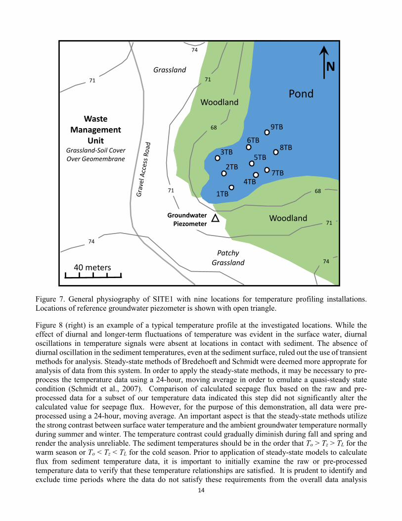
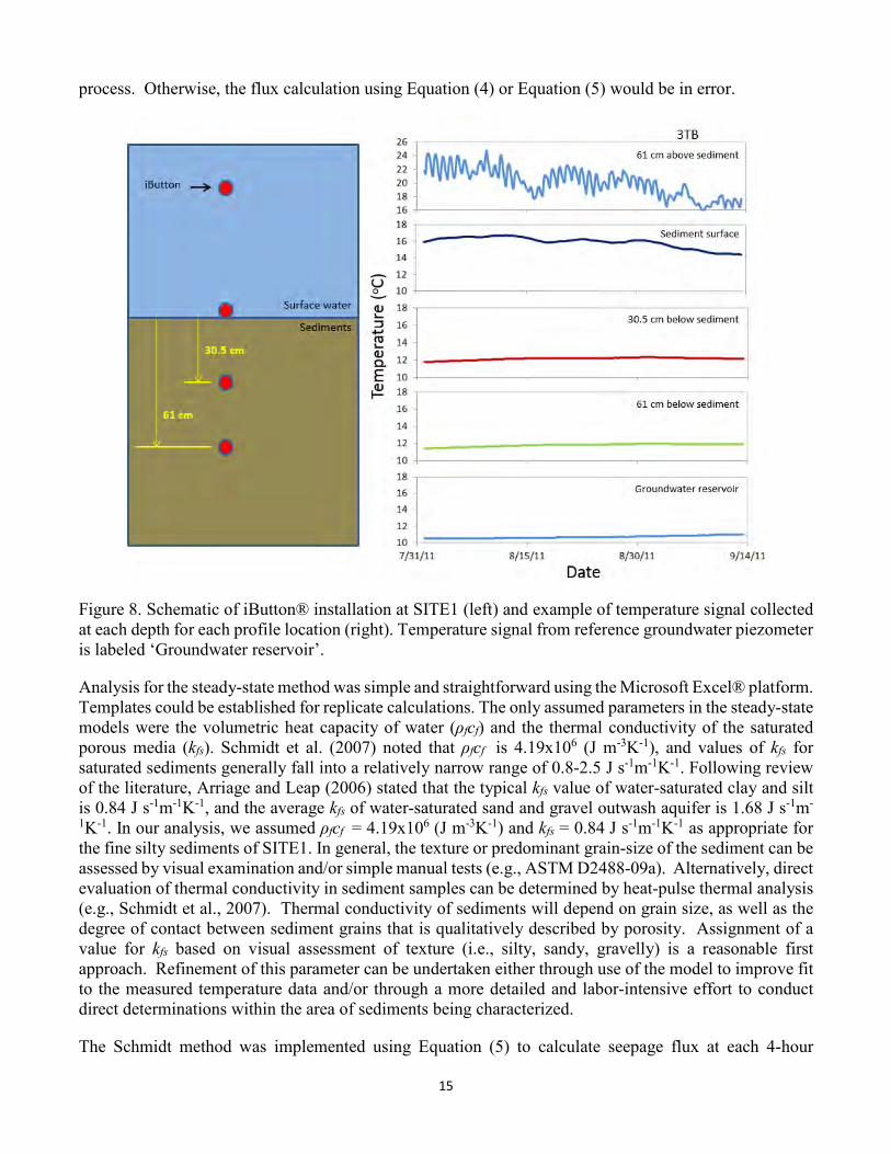
Figure 6 shows the schematic of an installation device used to drive each encapsulated iButton® to desired depth below the sediment surface. The iButton® temperature logger was securely seated inside the capsule. Nine locations in SITE1 were targeted for seepage flux investigation (Figure 7). A vertical profile of temperature loggers was installed at each location as illustrated in Figure 8 (left). A temperature logger was also placed at the bottom of a 7-m deep neighboring piezometer to log the local groundwater temperature. All deployed temperature loggers were tethered to a steel pipe driven into the sediments using braided, stainless steel wire attached to the protective capsule. Each temperature logger was offset approximately 5-cm in horizontal placement to facilitate collapse of the sediment and ensure thermal isolation from preferential flow paths. The deployent period of the seepage flux investigation at SITE1 was August 1 – September 13, 2011. At the conclusion of field deployment, all temperature loggers were retrieved for data download. The raw data were extracted from each individual iButton® into a NexSens micro-T database, then exported and saved in a Microsoft Excel® file format. The resultant data matrix included sampling date and time, iButton® identification number, deployment depth, deployment identification code, and raw temperature data.

13

Figure 6. Design schematic of iButton® installation device constructed using readily-available plumbing materials.

14

Figure 7. General physiography of SITE1 with nine locations for temperature profiling installations. Locations of reference groundwater piezometer is shown with open triangle.

Figure 8 (right) is an example of a typical temperature profile at the investigated locations. While the effect of diurnal and longer-term fluctuations of temperature was evident in the surface water, diurnal oscillations in temperature signals were absent at locations in contact with sediment. The absence of diurnal oscillation in the sediment temperatures, even at the sediment surface, ruled out the use of transient methods for analysis. Steady-state methods of Bredehoeft and Schmidt were deemed more approprate for analysis of data from this system. In order to apply the steady-state methods, it may be necessary to pre-process the temperature data using a 24-hour, moving average in order to emulate a quasi-steady state condition (Schmidt et al., 2007). Comparison of calculated seepage flux based on the raw and pre-processed data for a subset of our temperature data indicated this step did not significantly alter the calculated value for seepage flux. However, for the purpose of this demonstration, all data were pre-processed using a 24-hour, moving average. An important aspect is that the steady-state methods utilize the strong contrast between surface water temperature and the ambient groundwater temperature normally during summer and winter. The temperature contrast could gradually diminish during fall and spring and render the analysis unreliable. The sediment temperatures should be in the order that To > Tz > TL for the warm season or To < Tz < TL for the cold season. Prior to application of steady-state models to calculate flux from sediment temperature data, it is important to initially examine the raw or pre-processed temperature data to verify that these temperature relationships are satisfied. It is prudent to identify and exclude time periods where the data do not satisfy these requirements from the overall data analysis

40 meters

WasteManagement

UnitGrassland-Soil CoverOver Geomembrane

9TB

8TB6TB

5TB

7TB4TB

1TB

2TB

3TB

Pond

PatchyGrassland

Grassland

74

WoodlandGroundwaterPiezometer

71

68

71

74

71

74

71

68

Woodland

N

15

process. Otherwise, the flux calculation using Equation (4) or Equation (5) would be in error.

Figure 8. Schematic of iButton® installation at SITE1 (left) and example of temperature signal collected at each depth for each profile location (right). Temperature signal from reference groundwater piezometer is labeled ‘Groundwater reservoir’.

Analysis for the steady-state method was simple and straightforward using the Microsoft Excel® platform. Templates could be established for replicate calculations. The only assumed parameters in the steady-state models were the volumetric heat capacity of water (ρfcf) and the thermal conductivity of the saturated porous media (kfs). Schmidt et al. (2007) noted that ρfcf is 4.19x106 (J m-3K-1), and values of kfs for saturated sediments generally fall into a relatively narrow range of 0.8-2.5 J s-1m-1K-1. Following review of the literature, Arriage and Leap (2006) stated that the typical kfs value of water-saturated clay and silt is 0.84 J s-1m-1K-1, and the average kfs of water-saturated sand and gravel outwash aquifer is 1.68 J s-1m-

1K-1. In our analysis, we assumed ρfcf = 4.19x106 (J m-3K-1) and kfs = 0.84 J s-1m-1K-1 as appropriate for the fine silty sediments of SITE1. In general, the texture or predominant grain-size of the sediment can be assessed by visual examination and/or simple manual tests (e.g., ASTM D2488-09a). Alternatively, direct evaluation of thermal conductivity in sediment samples can be determined by heat-pulse thermal analysis (e.g., Schmidt et al., 2007). Thermal conductivity of sediments will depend on grain size, as well as the degree of contact between sediment grains that is qualitatively described by porosity. Assignment of a value for kfs based on visual assessment of texture (i.e., silty, sandy, gravelly) is a reasonable first approach. Refinement of this parameter can be undertaken either through use of the model to improve fit to the measured temperature data and/or through a more detailed and labor-intensive effort to conduct direct determinations within the area of sediments being characterized.

The Schmidt method was implemented using Equation (5) to calculate seepage flux at each 4-hour

16

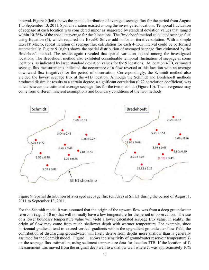
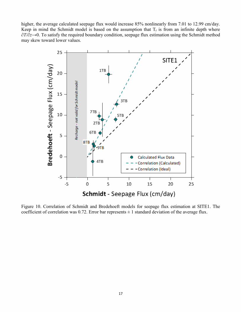
interval. Figure 9 (left) shows the spatial distribution of averaged seepage flux for the period from August 1 to September 13, 2011. Spatial variation existed among the investigated locations. Temporal fluctuation of seepage at each location was considered minor as suggested by standard deviation values that ranged within 10-36% of the absolute average for the 9 locations. The Bredehoeft method calculated seepage flux using Equation (5), which required the Excel® Solver add-in for an iterative solution. With a simple Excel® Macro, repeat iteration of seepage flux calculation for each 4-hour interval could be performed automatically. Figure 9 (right) shows the spatial distribution of averaged seepage flux estimated by the Bredehoeft method. The results again revealed that spatial variation existed among the investigated locations. The Bredehoeft method also exhibited considerable temporal fluctuation of seepage at some locations, as indicated by large standard deviation values for the 9 locations. At location 4TB, estimated seepage flux measurements indicated the occurrence of a flow reversal at this location with an average downward flux (negative) for the period of observation. Correspondingly, the Schmidt method also yielded the lowest seepage flux at the 4TB location. Although the Schmidt and Bredehoeft methods produced dissimilar results to a certain degree, a significant correlation (0.72 correlation coefficient) was noted between the estimated average seepage flux for the two methods (Figure 10). The divergence may come from different inherent assumptions and boundary conditions of the two methods.

Figure 9. Spatial distribution of averaged seepage flux (cm/day) at SITE1 during the period of August 1, 2011 to September 13, 2011.

For the Schmidt model it was assumed that the origin of the upward flow was from a deep groundwater reservoir (e.g., 5-10 m) that will normally have a low temperature for the period of observation. The use of a lower boundary temperature value will yield a lower calculated seepage flux value. In reality, the origin of flow may come from much shallower depth with warmer temperature. For example, since horizontal gradients tend to exceed vertical gradients within the upgradient groundwater flow field, the contribution of discharging groundwater will likely derive from depths more shallow than is generally assumed for the Schmidt model. Figure 11 shows the sensitivity of groundwater reservoir temperature Tr on the seepage flux estimation, using sediment temperature data for location 3TB. If the location of Tr measurement was moved from the original deep well to a shallow well where Tr was approximately 10%

17

higher, the average calculated seepage flux would increase 85% nonlinearly from 7.01 to 12.99 cm/day. Keep in mind the Schmidt model is based on the assumption that Tr is from an infinite depth where ∂T/∂z→0. To satisfy the required boundary condition, seepage flux estimation using the Schmidt method may skew toward lower values.

Figure 10. Correlation of Schmidt and Bredehoeft models for seepage flux estimation at SITE1. The coefficient of correlation was 0.72. Error bar represents ± 1 standard deviation of the average flux.

18

Figure 11. A hypothetical example on the 3TB location showing percent increase in seepage flux estimation as a function of percentage increase in the reference groundwater temperature (Tr) used in the Schmidt model.

3.2 Transient Method Example

As part of the post remedial site characterization effort, a seepage flux investigation was carried out at a flowing river site (referred to as SITE2 herein). At the time of the investigation, the river had been restored by dredging and subsequently protected by a cap cover consisting dominantly of sandy material, but inclusive of materials ranging in texture from silty to gravelly. The objective of this evaluation was to determine the spatial and temporal variation of the magnitude and direction of the seepage flux along a transect perpendicular to the river flow. Five equally spaced locations along the targeted transect were investigated (Figure 12). The entire river channel shown in this figure had been dredged and capped. The temperature method was chosen as an indirect approach for the seepage flux study. The deployment of iButton® as the temperature logger was similar to the approach described for SITE1. Figure 13 (left) illustrates the schematic of iButton® installations at SITE2. In order to avoid penetration through the protective cap and risk compromising its integrity, the installation was limited to the top 20 cm of the cap. Prior to the installation, all temperature loggers were synchronized for time and sampling interval and were programmed to begin data logging at the same date and time with a 4-hour sampling interval. All deployed temperature loggers were tethered to a plastic-coated, braided wire cable stretched across the river channel and anchored to each shoreline. As at SITE1, the tether consisted of braided, stainless steel wire attached to the protective capsule.The deployment period of the seepage flux investigation at SITE2 was June 24 – July 29, 2012. At the conclusion of field deployment, all temperature loggers were retrieved for data download. The raw data were extracted from each individual iButton® into a NexSens micro-T database, then exported and saved in a Microsoft Excel® file format.

19

Figure 22. Seepage flux investigation locations at SITE2. The entire reach of the river shown in this view was dredged and subsequently capped.

Figure 13 (right) is an example of a typical sediment temperature profile at the investigated locations. The seasonal and diurnal effect on temperature fluctuation was evident at all three observation depths. The display of diurnal oscillation in the sediment temperatures suggested that the use of transient method for seepage flux estimation was more desirable than the steady-state method. The analysis of the transient time-series method was not as straightforward as the steady-state method. First, each cycle of the raw temperature time-series was best-fit to Equation (13) with four harmonic components to ensure a creditable fit. Fuggle (1971) suggested that 98% of the variation in temperature is related to the first two harmonics of the series. The sum of four harmonic components was considered adequate to depict the raw temperature signals observed at SITE2. Secondly, the 1st harmonic component of the regression fit was extracted to determine the amplitude and phase angle of each diurnal cycle using Equation (14) and Equation (15), or determined graphically from the temperature maxima or minima of the diurnal sinusoidal cycle. Thirdly, matched amplitude pairs from the time-series signal were used to calculate amplitude ratios and phase shifts using Equation (16) and Equation (17). And finally, the Keery and/or Hatch models were used to estimate daily seepage flux value using the amplitude ratio or phase shift. Unlike the steady-state methods where seepage flux can be determined for each 4-hour sampling interval, the time-series methods only yield one flux value per diurnal cycle (24 hour period). The underlying assumption is that although seepage fluxes in many natural systems will vary continuously and slowly over days to weeks or more (Hatch et al., 2006), the seepage flux is assumed constant throughout the period of a diurnal cycle when using the time-series method. Hatch et al. (2006) concluded that the time-series method is sensitive to abrupt changes in seepage rates and directions, and the significance of this limitation depends on the magnitude and frequency of seepage flux variations.

20 meters

WT5WT4

WT3

WT2

WT1

River

N

20

Figure 33. Schematic of iButton® installation at SITE2 (left), and example of typical corresponding temperature profile at SITE2 location (right).

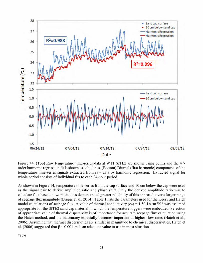
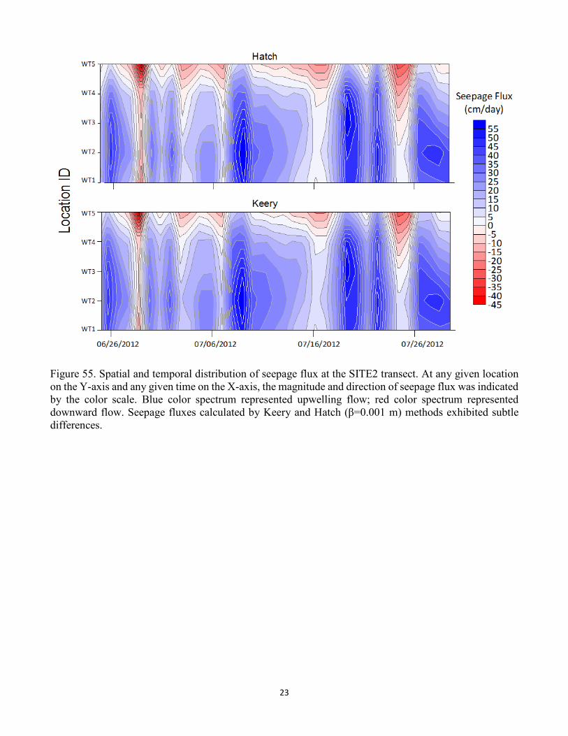
Figure 14 (top) is an example of 4th-order harmonic regression fit of raw temperature time-series for the two different depths. The harmonic regression model fitted the raw temperature time-series convincingly. The overall quality of the regression fit was good, as indicated by values for R2 of 0.988 and 0.996 for the temperature time-series at the cap surface and 10 cm below cap, respectively. Figure 14 (bottom) exhibits the 1st harmonic components of the two time-series extracted from the above harmonic regression. A decrease in amplitude and time lag were observed at the deeper of the two depths. The amplitude ratio and phase shift of the signal pair can then be determined from the two corresponding diurnal cycles.

21

Figure 44. (Top) Raw temperature time-series data at WT1 SITE2 are shown using points and the 4th-order harmonic regression fit is shown as solid lines. (Bottom) Diurnal (first harmonic) components of the temperature time-series signals extracted from raw data by harmonic regression. Extracted signal for whole period consists of individual fits to each 24-hour period.

As shown in Figure 14, temperature time-series from the cap surface and 10 cm below the cap were used as the signal pair to derive amplitude ratio and phase shift. Only the derived amplitude ratio was to calculate flux based on work that has demonstrated greater reliability of this approach over a larger range of seepage flux magnitude (Briggs et al., 2014). Table 1 lists the parameters used for the Keery and Hatch model calculations of seepage flux. A value of thermal conductivity (kfs) = 1.50 J s-1m-1K-1 was assumed appropriate for the SITE2 sand cap material in which the temperature loggers were embedded. Selection of appropriate value of thermal dispersivity is of importance for accurate seepage flux calculation using the Hatch method, and the inaccuracy especially becomes important at higher flow rates (Hatch et al., 2006). Assuming that thermal dispersivities are similar in magnitude to chemical dispersivities, Hatch et al. (2006) suggested that β ~ 0.001-m is an adequate value to use in most situations.

Table

22

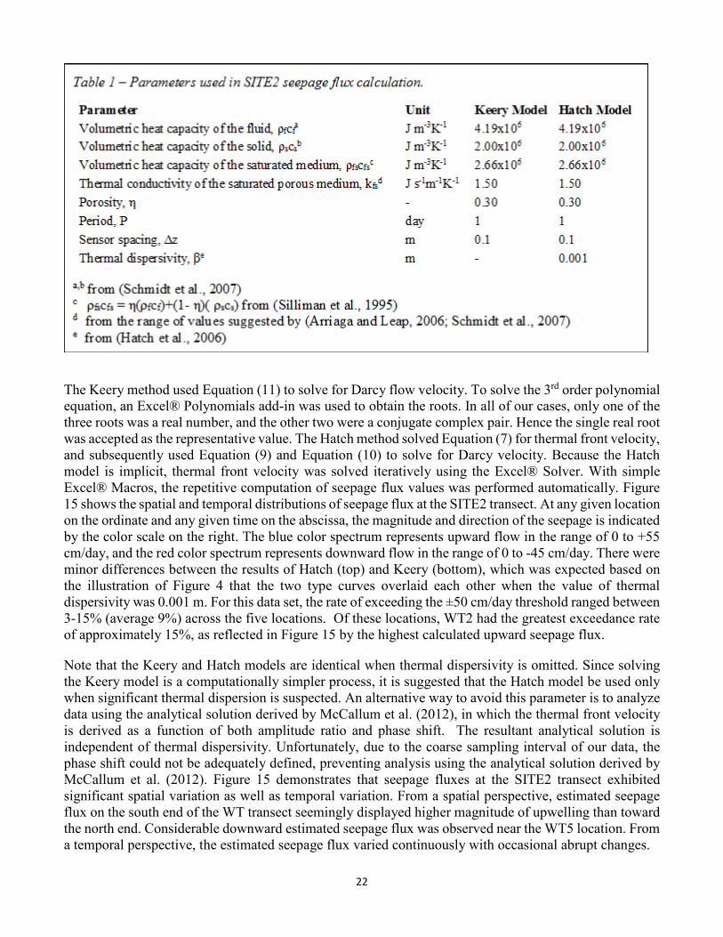
The Keery method used Equation (11) to solve for Darcy flow velocity. To solve the 3rd order polynomial equation, an Excel® Polynomials add-in was used to obtain the roots. In all of our cases, only one of the three roots was a real number, and the other two were a conjugate complex pair. Hence the single real root was accepted as the representative value. The Hatch method solved Equation (7) for thermal front velocity, and subsequently used Equation (9) and Equation (10) to solve for Darcy velocity. Because the Hatch model is implicit, thermal front velocity was solved iteratively using the Excel® Solver. With simple Excel® Macros, the repetitive computation of seepage flux values was performed automatically. Figure 15 shows the spatial and temporal distributions of seepage flux at the SITE2 transect. At any given location on the ordinate and any given time on the abscissa, the magnitude and direction of the seepage is indicated by the color scale on the right. The blue color spectrum represents upward flow in the range of 0 to +55 cm/day, and the red color spectrum represents downward flow in the range of 0 to -45 cm/day. There were minor differences between the results of Hatch (top) and Keery (bottom), which was expected based on the illustration of Figure 4 that the two type curves overlaid each other when the value of thermal dispersivity was 0.001 m. For this data set, the rate of exceeding the ±50 cm/day threshold ranged between 3-15% (average 9%) across the five locations. Of these locations, WT2 had the greatest exceedance rate of approximately 15%, as reflected in Figure 15 by the highest calculated upward seepage flux.

Note that the Keery and Hatch models are identical when thermal dispersivity is omitted. Since solving the Keery model is a computationally simpler process, it is suggested that the Hatch model be used only when significant thermal dispersion is suspected. An alternative way to avoid this parameter is to analyze data using the analytical solution derived by McCallum et al. (2012), in which the thermal front velocity is derived as a function of both amplitude ratio and phase shift. The resultant analytical solution is independent of thermal dispersivity. Unfortunately, due to the coarse sampling interval of our data, the phase shift could not be adequately defined, preventing analysis using the analytical solution derived by McCallum et al. (2012). Figure 15 demonstrates that seepage fluxes at the SITE2 transect exhibited significant spatial variation as well as temporal variation. From a spatial perspective, estimated seepage flux on the south end of the WT transect seemingly displayed higher magnitude of upwelling than toward the north end. Considerable downward estimated seepage flux was observed near the WT5 location. From a temporal perspective, the estimated seepage flux varied continuously with occasional abrupt changes.

23

Figure 55. Spatial and temporal distribution of seepage flux at the SITE2 transect. At any given location on the Y-axis and any given time on the X-axis, the magnitude and direction of seepage flux was indicated by the color scale. Blue color spectrum represented upwelling flow; red color spectrum represented downward flow. Seepage fluxes calculated by Keery and Hatch (β=0.001 m) methods exhibited subtle differences.

24

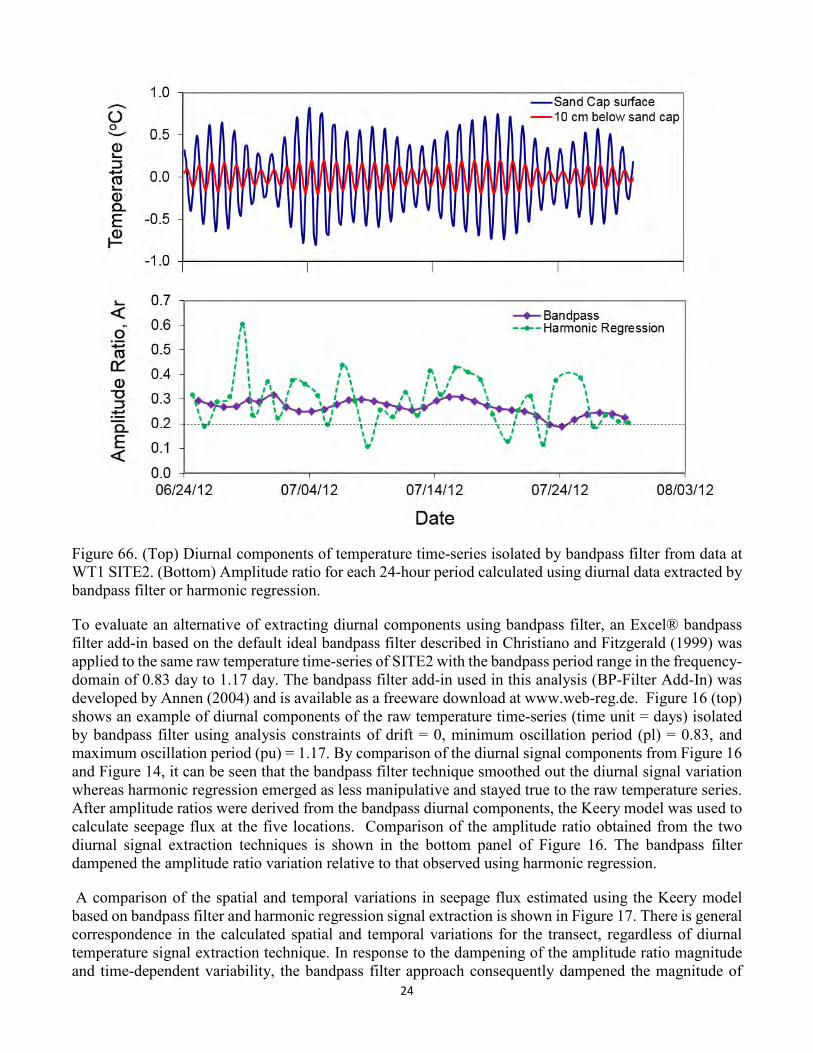
Figure 66. (Top) Diurnal components of temperature time-series isolated by bandpass filter from data at WT1 SITE2. (Bottom) Amplitude ratio for each 24-hour period calculated using diurnal data extracted by bandpass filter or harmonic regression.

To evaluate an alternative of extracting diurnal components using bandpass filter, an Excel® bandpass filter add-in based on the default ideal bandpass filter described in Christiano and Fitzgerald (1999) was applied to the same raw temperature time-series of SITE2 with the bandpass period range in the frequency-domain of 0.83 day to 1.17 day. The bandpass filter add-in used in this analysis (BP-Filter Add-In) was developed by Annen (2004) and is available as a freeware download at www.web-reg.de. Figure 16 (top) shows an example of diurnal components of the raw temperature time-series (time unit = days) isolated by bandpass filter using analysis constraints of drift = 0, minimum oscillation period (pl) = 0.83, and maximum oscillation period (pu) = 1.17. By comparison of the diurnal signal components from Figure 16 and Figure 14, it can be seen that the bandpass filter technique smoothed out the diurnal signal variation whereas harmonic regression emerged as less manipulative and stayed true to the raw temperature series. After amplitude ratios were derived from the bandpass diurnal components, the Keery model was used to calculate seepage flux at the five locations. Comparison of the amplitude ratio obtained from the two diurnal signal extraction techniques is shown in the bottom panel of Figure 16. The bandpass filter dampened the amplitude ratio variation relative to that observed using harmonic regression.

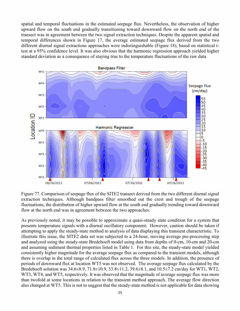
A comparison of the spatial and temporal variations in seepage flux estimated using the Keery model based on bandpass filter and harmonic regression signal extraction is shown in Figure 17. There is general correspondence in the calculated spatial and temporal variations for the transect, regardless of diurnal temperature signal extraction technique. In response to the dampening of the amplitude ratio magnitude and time-dependent variability, the bandpass filter approach consequently dampened the magnitude of

25

spatial and temporal fluctuations in the estimated seepage flux. Nevertheless, the observation of higher upward flow on the south end gradually transitioning toward downward flow on the north end of the transect was in agreement between the two signal extraction techniques. Despite the apparent spatial and temporal differences shown in Figure 17, the average estimated seepage flux derived from the two different diurnal signal extractions approaches were indistinguishable (Figure 18), based on statistical t-test at a 95% confidence level. It was also obvious that the harmonic regression approach yielded higher standard deviation as a consequence of staying true to the temperature fluctuations of the raw data.

Figure 77. Comparison of seepage flux of the SITE2 transect derived from the two different diurnal signal extraction techniques. Although bandpass filter smoothed out the crest and trough of the seepage fluctuations, the distribution of higher upward flow at the south end gradually trending toward downward flow at the north end was in agreement between the two approaches.

As previously noted, it may be possible to approximate a quasi-steady state condition for a system that presents temperature signals with a diurnal oscillatory component. However, caution should be taken if attempting to apply the steady-state method to analysis of data displaying this transient characteristic. To illustrate this issue, the SITE2 data set was subjected to a 24-hour, moving average pre-processing step and analyzed using the steady-state Bredehoeft model using data from depths of 0-cm, 10-cm and 20-cm and assuming sediment thermal properties listed in Table 1. For this site, the steady-state model yielded consistently higher magnitude for the average seepage flux as compared to the transient models, although there is overlap in the total range of calculated flux across the three models. In addition, the presence of periods of downward flux at location WT5 was not observed. The average seepage flux calculated by the Bredehoeft solution was 34.6±8.9, 71.0±10.9, 33.8±11.2, 39.6±8.1, and 10.5±7.2 cm/day for WT1, WT2, WT3, WT4, and WT5, respectively. It was observed that the magnitude of average seepage flux was more than twofold at some locations in relation to the transient method approach. The average flow direction also changed at WT5. This is not to suggest that the steady-state method is not applicable for data showing

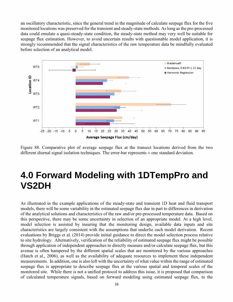
26

an oscillatory characteristic, since the general trend in the magnitude of calculate seepage flux for the five monitored locations was preserved for the transient and steady-state methods. As long as the pre-processed data could emulate a quasi-steady-state condition, the steady-state method may very well be suitable for seepage flux estimation. However, to avoid uncertain results with questionable model application, it is strongly recommended that the signal characteristics of the raw temperature data be mindfully evaluated before selection of an analytical model.

Figure 88. Comparative plot of average seepage flux at the transect locations derived from the two different diurnal signal isolation techniques. The error-bar represents ± one standard deviation.

4.0 Forward Modeling with 1DTempPro and VS2DH

As illustrated in the example applications of the steady-state and transient 1D heat and fluid transport models, there will be some variability in the estimated seepage flux due in part to differences in derivation of the analytical solutions and characteristics of the raw and/or pre-processed temperature data. Based on this perspective, there may be some uncertainty in selection of an appropriate model. At a high level, model selection is assisted by insuring that the monitoring design, available data inputs and site characteristics are largely consistent with the assumptions that underlie each model derivation. Recent evaluations by Briggs et al. (2014) provide initial guidance to direct the model selection process relative to site hydrology. Alternatively, verification of the reliability of estimated seepage flux might be possible through application of independent approaches to directly measure and/or calculate seepage flux, but this avenue is often hampered by the different spatial scales that are monitored by the various approaches (Hatch et al., 2006), as well as the availability of adequate resources to implement these independent measurements. In addition, one is also left with the uncertainty of what value within the range of estimated seepage flux is appropriate to describe seepage flux at the various spatial and temporal scales of the monitored site. While there is not a unified protocol to address this issue, it is proposed that comparison of calculated temperature signals, based on forward modeling using estimated seepage flux, to the

27

observed temperature signal at different locations and time period provides a means to make a qualitative and semi-quantitative assessment of the degree of accuracy of estimated seepage flux derived from application of the inverse, one-dimensional heat and fluid transport models.

The U.S. Geological Survey computer code entitled Variably Saturated 2-Dimensional Heat Transport (VS2DH) numerically simulates fluid flow and heat-transport in saturated porous media. VS2DH is useful in modeling the near-surface transport of water and heat in porous sediments for cases in which transport in the vapor phase and density variations are negligible (Healy and Ronan, 1996). While quantifying seepage flux from sediment temperatures is an inverse process that derives the magnitude and direction of seepage from the measured temperatures, modeling with VS2DH is a forward process that predicts the temporal pattern of sediment temperatures from the given hydraulic and thermal properties. By comparing the forward-model prediction to the measured temperature, forward modeling can be used as a tool to evaluate the appropriateness of the seepage flux estimated using the inverse model.

Forward modeling in one dimension with VS2DH was carried out using a graphical user interface program, 1DTempPro (Version 1.0.1.2; Voytek et al., 2013), for the simulation of vertical one-dimensional temperature profiles under saturated flow conditions. At both SITE1 and SITE2, sediment temperature were measured at three different depths (Figure 8, Figure 13). For application of these verification checks, temperature time-series from the shallowest and deepest monitored depths were used as input boundary conditions within 1DTempPro with internal calculation, using VS2DH, of the temperature at the intermediate monitored depth. The same sediment thermal parameters as used for the one-dimensional inverse models were used for calculations by VS2DH. Average seepage flux at each location was calculated from the seepage flux time-series estimated by the inverse method (presented in Figure 9 and Figure 15), and entered as one of the 1DTempPro input parameters. (Note that this approach does not address the reliability of the temporal distribution of estimated seepage flux derived from the inverse modeling approaches.) The VS2DH model generated a predicted temperature time-series for the intermediate depth, and a calculated root mean square error (RMSE) as a measure of the difference between predicted and measured temperatures. The accuracy of the inverse-method seepage flux estimate increases with decreasing value of the forward model RMSE, as previously illustrated by Rau et al. (2010). As suggested by Briggs et al. (2013), the minimum value of RMSE will be limited by the resolution of the temperature datalogger.

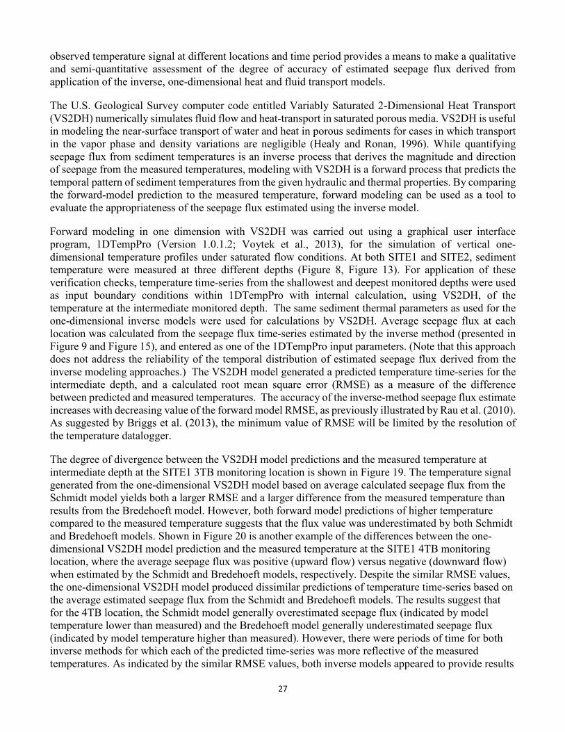
The degree of divergence between the VS2DH model predictions and the measured temperature at intermediate depth at the SITE1 3TB monitoring location is shown in Figure 19. The temperature signal generated from the one-dimensional VS2DH model based on average calculated seepage flux from the Schmidt model yields both a larger RMSE and a larger difference from the measured temperature than results from the Bredehoeft model. However, both forward model predictions of higher temperature compared to the measured temperature suggests that the flux value was underestimated by both Schmidt and Bredehoeft models. Shown in Figure 20 is another example of the differences between the one-dimensional VS2DH model prediction and the measured temperature at the SITE1 4TB monitoring location, where the average seepage flux was positive (upward flow) versus negative (downward flow) when estimated by the Schmidt and Bredehoeft models, respectively. Despite the similar RMSE values, the one-dimensional VS2DH model produced dissimilar predictions of temperature time-series based on the average estimated seepage flux from the Schmidt and Bredehoeft models. The results suggest that for the 4TB location, the Schmidt model generally overestimated seepage flux (indicated by model temperature lower than measured) and the Bredehoeft model generally underestimated seepage flux (indicated by model temperature higher than measured). However, there were periods of time for both inverse methods for which each of the predicted time-series was more reflective of the measured temperatures. As indicated by the similar RMSE values, both inverse models appeared to provide results

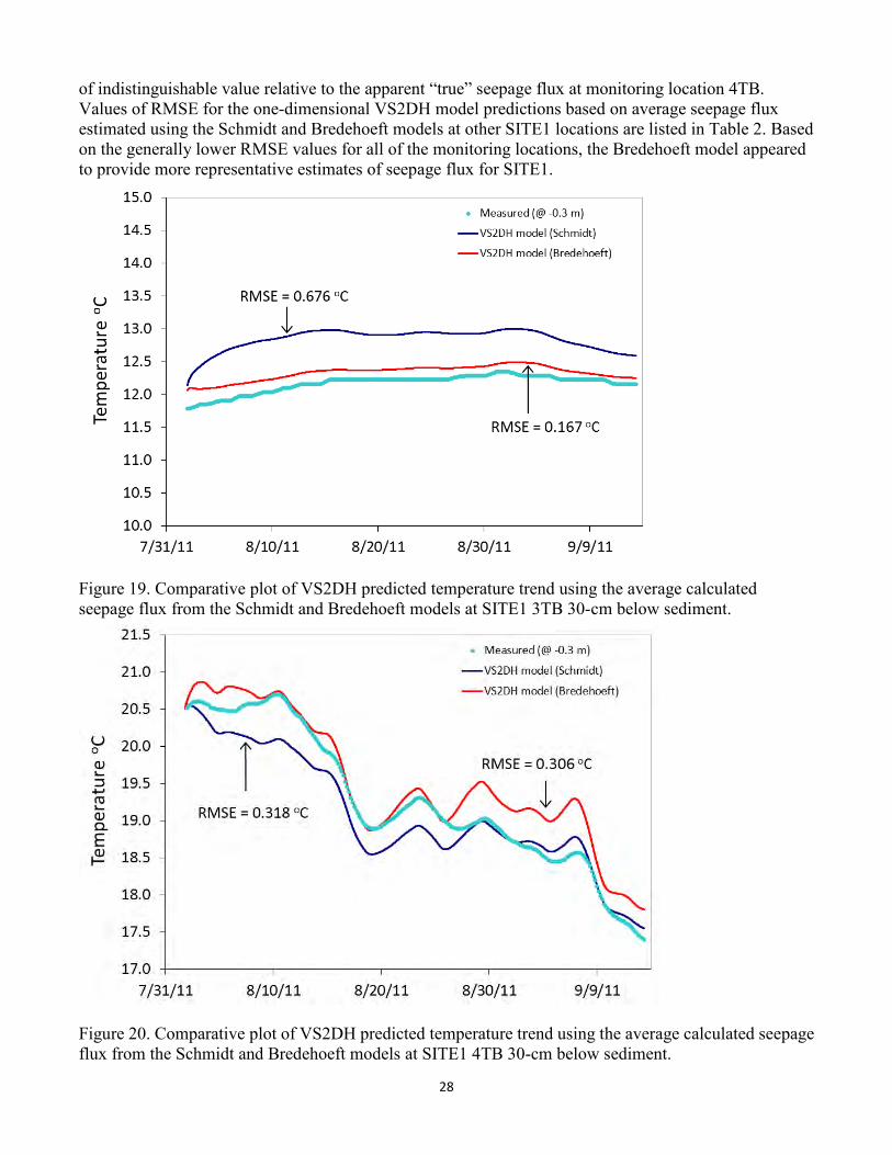
28

of indistinguishable value relative to the apparent “true” seepage flux at monitoring location 4TB. Values of RMSE for the one-dimensional VS2DH model predictions based on average seepage flux estimated using the Schmidt and Bredehoeft models at other SITE1 locations are listed in Table 2. Based on the generally lower RMSE values for all of the monitoring locations, the Bredehoeft model appeared to provide more representative estimates of seepage flux for SITE1.

Figure 19. Comparative plot of VS2DH predicted temperature trend using the average calculated seepage flux from the Schmidt and Bredehoeft models at SITE1 3TB 30-cm below sediment.

Figure 20. Comparative plot of VS2DH predicted temperature trend using the average calculated seepage flux from the Schmidt and Bredehoeft models at SITE1 4TB 30-cm below sediment.

29

The degree of divergence between the VS2DH model predictions and the measured temperature at intermediate depth at the SITE2 WT1 monitoring location is shown in Figure 21. The model temperature derived using the average seepage flux from the Keery and Hatch models were practically identical, and convincingly matched the measured temperature. Values of RMSE for VS2DH model predictions based on average seepage flux estimated using the Keery and Hatch models at other SITE2 locations are listed in Table 2. In general, both transient methods appeared to provide reliable estimates of average seepage flux that yielded small RMSE in forward modeling verification. Omission of thermal dispersivity in the Keery model did not affect the outcome of the VS2DH evaluation. Forward modeling was also used to evaluate the influence of a change in the value of thermal conductivity on calculated seepage flux. The Keery model was run again using a value of kfs = 0.61 J s-1m-1K-1, which resulted in calculated flux values of 0.3±9.5, 3.0±9.7, 0.4±9.3, -2.4±8.9, and -14.1±9.1 cm/day for locations WT1, WT2, WT3, WT4 and WT5, respectively. The factor-of-three reduction in the value of thermal conductivity resulted in an approximate three-order-of-magnitude reduction in calculated seepage flux. However, the new average calculated seepage flux values for locations WT1 and WT5 were re-evaluated by forward modeling with VS2DH in combination with a value of kfs = 0.61 J s-1m-1K-1. The outcome of this test showed a degradation in the resultant temperature trend prediction with new goodness-of-fit values for RMSE of 0.209°C and 0.250°C for WT1 and WT5, respectively. In both cases, the new average seepage flux values and kfs resulted in a predicted temperature trend with values higher than the measured temperature, which is consistent with an underestimate of the seepage flux at both locations. This analysis demonstrates the importance of selecting a reasonable value for thermal conductivity, and the utility of using forward modeling with VS2DH to assess reliability for this parameter.

To examine the appropriateness of applying a steady-state model on transient characteristic data of SITE2, the average seepage flux derived from the Bredehoeft method was also evaluated at each monitoring location by application of the one-dimensional VS2DH model via 1DTempPro. Figure 22 is a comparative plot of one-dimensional VS2DH predictions, using the Keery and Bredehoeft method estimated average fluxes, versus the measured temperature at 10-cm below the sand cap for the WT5 monitoring location. Both 1DTempPro model predictions matched the measured temperature data reasonably well in terms of magnitude and oscillation. The RMSE results indicate a slight improvement based on average seepage flux derived from the transient, Keery method. Values of RMSE from the one-dimensional VS2DH model prediction based on average seepage flux derived from the steady-state, Bredehoeft method for other SITE2 locations are also listed in Table 2. Examination of the value of RMSE calculated for a period of record during which the average temperature at the intermediate depth was more stable (i.e., July 20-30), resulted in the same trend in apparent goodness-of-fit for the transient and steady-state model shown in Table 2. With an approximate order-of-magnitude difference in the average calculated seepage flux from these two models for location WT5, the results shown in Table 2 indicate that the calculations implemented within 1DTempPro (Version 1.0.1.2) are relatively insensitive to this input parameter or are potentially limited by the resolution of the temperature loggers used in this study (resolution approximately 0.06°C). Based on the fit results presented in Table 2, one would be hard-pressed to suggest that the steady-state method of Bredehoeft is not suitable for the SITE2 data. However, a conclusive verdict on the appropriateness of applying steady-state model(s) on transient characteristic data would require further evaluation from more data sets collected under a wider variety of physical settings.

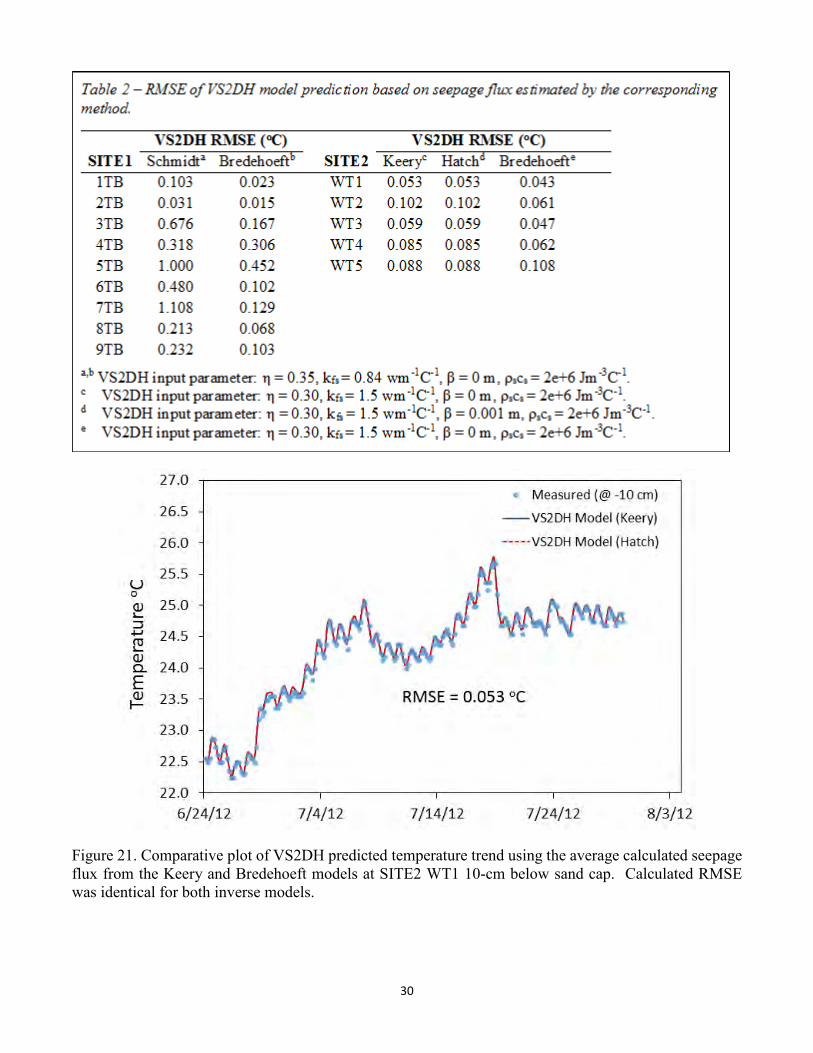
30

Figure 21. Comparative plot of VS2DH predicted temperature trend using the average calculated seepage flux from the Keery and Bredehoeft models at SITE2 WT1 10-cm below sand cap. Calculated RMSE was identical for both inverse models.

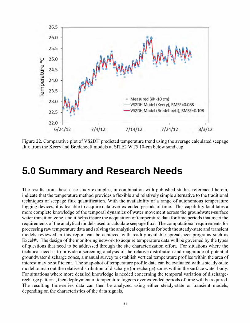
31

Figure 22. Comparative plot of VS2DH predicted temperature trend using the average calculated seepage flux from the Keery and Bredehoeft models at SITE2 WT5 10-cm below sand cap.

5.0 Summary and Research Needs

The results from these case study examples, in combination with published studies referenced herein, indicate that the temperature method provides a flexible and relatively simple alternative to the traditional techniques of seepage flux quantification. With the availability of a range of autonomous temperature logging devices, it is feasible to acquire data over extended periods of time. This capability facilitates a more complete knowledge of the temporal dynamics of water movement across the groundwater-surface water transition zone, and it helps insure the acquisition of temperature data for time periods that meet the requirements of the analytical models used to calculate seepage flux. The computational requirements for processing raw temperature data and solving the analytical equations for both the steady-state and transient models reviewed in this report can be achieved with readily available spreadsheet programs such as Excel®. The design of the monitoring network to acquire temperature data will be governed by the types of questions that need to be addressed through the site characterization effort. For situations where the technical need is to provide a screening analysis of the relative distribution and magnitude of potential groundwater discharge zones, a manual survey to establish vertical temperature profiles within the area of interest may be sufficient. The snap-shot of temperature profile data can be evaluated with a steady-state model to map out the relative distribution of discharge (or recharge) zones within the surface water body. For situations where more detailed knowledge is needed concerning the temporal variation of discharge-recharge patterns, then deployment of temperature loggers over extended periods of time will be required. The resulting time-series data can then be analyzed using either steady-state or transient models, depending on the characteristics of the data signals.

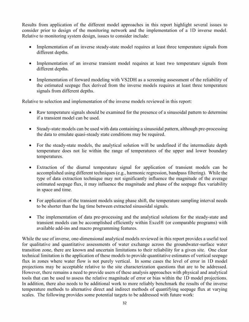
32

Results from application of the different model approaches in this report highlight several issues to consider prior to design of the monitoring network and the implementation of a 1D inverse model. Relative to monitoring system design, issues to consider include:

• Implementation of an inverse steady-state model requires at least three temperature signals from different depths.

• Implementation of an inverse transient model requires at least two temperature signals from different depths.

• Implementation of forward modeling with VS2DH as a screening assessment of the reliability of the estimated seepage flux derived from the inverse models requires at least three temperature signals from different depths.

Relative to selection and implementation of the inverse models reviewed in this report:

• Raw temperature signals should be examined for the presence of a sinusoidal pattern to determine if a transient model can be used.

• Steady-state models can be used with data containing a sinusoidal pattern, although pre-processing the data to emulate quasi-steady state conditions may be required.

• For the steady-state models, the analytical solution will be undefined if the intermediate depth temperature does not lie within the range of temperatures of the upper and lower boundary temperatures.

• Extraction of the diurnal temperature signal for application of transient models can be accomplished using different techniques (e.g., harmonic regression, bandpass filtering). While the type of data extraction technique may not significantly influence the magnitude of the average estimated seepage flux, it may influence the magnitude and phase of the seepage flux variability in space and time.

• For application of the transient models using phase shift, the temperature sampling interval needs to be shorter than the lag time between extracted sinusoidal signals.

• The implementation of data pre-processing and the analytical solutions for the steady-state and transient models can be accomplished efficiently within Excel® (or comparable programs) with available add-ins and macro programming features.

While the use of inverse, one-dimensional analytical models reviewed in this report provides a useful tool for qualitative and quantitative assessments of water exchange across the groundwater-surface water transition zone, there are known and uncertain limitations to their reliability for a given site. One clear technical limitation is the application of these models to provide quantitative estimates of vertical seepage flux in zones where water flow is not purely vertical. In some cases the level of error in 1D model projections may be acceptable relative to the site characterization questions that are to be addressed. However, there remains a need to provide users of these analysis approaches with physical and analytical tools that can be used to assess the relative magnitude of error or bias within the 1D model projections. In addition, there also needs to be additional work to more reliably benchmark the results of the inverse temperature methods to alternative direct and indirect methods of quantifying seepage flux at varying scales. The following provides some potential targets to be addressed with future work:

33

• Development and validation of screening approaches, through indirect field measurements or data analysis procedures within the analytical model framework, to assess whether horizontal flow components may impede use of 1D, inverse models.

• Synthesis of studies with independent measures of seepage flux to support statistical evaluation of the accuracy of temperature-based measurements across a range of site conditions.

• A critical survey of direct measurements of sediment properties that are model inputs in order to help constrain the process of model input parameter value selection.

• Studies to provide better context for the importance of assessing temporal and spatial variability of seepage flux. It would be useful to have a decision framework that links desired use of seepage flux determinations to the types of data acquisition approaches that are needed.

While not an all-inclusive list of research needs, they are intended to focus future work towards facilitating the appropriate use of temperature monitoring to characterize and assess the importance of water flow across the groundwater-surface water transition zone in support of site restoration activities and watershed revitalization and protection decisions.

34

6.0 References Anderson, M.P., 2005. Heat as a ground water tracer. Ground Water, 43(6): 951-968. Anibas, C., Buis, K., Verhoeven, R., Meire, P. and Batelaan, O., 2011. A simple thermal mapping

method for seasonal spatial patterns of groundwater–surface water interaction. Journal of Hydrology, 397(1–2): 93-104.

Anibas, C., Fleckenstein, J.H., Volze, N., Buis, K., Verhoeven, R., Meire, P. and Batelaan, O., 2009. Transient or steady-state? Using vertical temperature profiles to quantify groundwater–surface water exchange. Hydrological Processes, 23(15): 2165-2177.

Annen, K., 2004. "Band-Pass Filter Excel® Add-in," QM&RBC Codes 164, Quantitative Macroeconomics & Real Business Cycles.

Arriaga, M. and Leap, D., 2006. Using solver to determine vertical groundwater velocities by temperature variations, Purdue University, Indiana, USA. Hydrogeology Journal, 14(1): 253-263.

ASTM D2488-09a., 2009. Standard Practice for Description and Identification of Soils (Visual-Manual Procedure), ASTM International, West Conshohocken, PA.

Baskaran, S., Brodie, R.S., Ransley, T. and Baker, P., 2009. Time-series measurements of stream and sediment temperature for understanding river–groundwater interactions: Border Rivers and Lower Richmond catchments, Australia. Australian Journal of Earth Sciences, 56(1): 21-30.

Bencala, K.E., 2006. Hyporheic Exchange Flows, Encyclopedia of Hydrological Sciences. John Wiley & Sons, Ltd.

Bredehoeft, J.D. and Papadopulos, I.S., 1965. Rates of vertical groundwater movement estimated from the Earth's thermal profile. Water Resour. Res., 1(2): 325-328.

Briggs, M.A., Lautz, L.K. and McKenzie, J.M., 2012a. A comparison of fibre-optic distributed temperature sensing to traditional methods of evaluating groundwater inflow to streams. Hydrological Processes, 26(9): 1277-1290.

Briggs, M.A., Lautz, L.K., McKenzie, J.M., Gordon, R.P. and Hare, D.K., 2012b. Using high-resolution distributed temperature sensing to quantify spatial and temporal variability in vertical hyporheic flux. Water Resour. Res., 48(2): W02527.

Briggs, M.A., Voytek, E.B., Day-Lewis, F., Rosenberry, D.O., and Lane, J.W., 2013. Understanding water column and streambed thermal refugia for endangered mussels in the Delaware River. Environ. Sci. Tech., 47(20): 11423-11431.

Briggs, M.A., Lautz, L.K., Buckley, S.F., and Lane, J.W., 2014. Practical limitations on the use of diurnal temperature signals to quantify groundwater upwelling. Journal of Hydrology, 519: 1739-1751.

Brookfield, A. and Sudicky, E., 2013. Implications of Hyporheic Flow on Temperature-Based Estimates of Groundwater/Surface Water Interactions. Journal of Hydrologic Engineering, 18(10): 1250-1261.

Cartwright, K., 1970. Groundwater Discharge in the Illinois Basin as Suggested by Temperature Anomalies. Water Resources Research, 6(3): 912-918.

Christiano, L.J. and Fitzgerald, T.J., 1999. The Band Pass Filter. NBER Working Papers 7257, National Bureau of Economic Research, Inc.

Conant, B., Jr., 2004. Delineating and quantifying ground water discharge zones using streambed temperatures. Ground Water, 42(2): 243-257.

Constantz, J., 2008. Heat as a tracer to determine streambed water exchanges. Water Resour. Res., 44: W00D10.

Cranswick, R.H., Cook, P.G., Shanafield, M., and Lamontagne, S., 2014. The vertical variability of hyporheic fluxes inferred from riverbed temperature data. Water Resour. Res., 50(5): 3994-4010.

35

Cuthbert, M.O. and Mackay, R., 2013. Impacts of nonuniform flow on estimates of vertical streambed flux. Water Resour. Res., 49: 19-28.

Davis, H.T., 1967. The Analysis of Economic Time-series, Chapter 2: The Technique of Harmonic Analysis, Bloomington, Ind., Principia Press.

de Marsily, G., 1986. Quantitative hydrogeology: groundwater hydrology for engineers. Academic Press.

Ferguson, G., 2007. Heterogeneity and thermal modeling of ground water. Ground Water, 45(4): 485-90.

Ferguson, G. and Bense, V., 2011. Uncertainty in 1D heat-flow analysis to estimate groundwater discharge to a stream. Groundwater, 49(3): 336-347.

Fuggle, R.F., 1971. A Note on the Harmonic Analysis of the Diurnal Temperature Waves at Three Locations on a Mountain Slope. South African Geographical Journal, 53(1): 93-95.

Gamble, D.W., Taborosi, D., Mylroie, J.E., Jenson, J.W., Carew, J.L., Jocson, J.M.U., Mylroie, J. and Vann, D.T., 2003. The use of water temperature to characterize groundwater discharge of a coastal fracture on Guam, USA. Journal of Coastal Research, 19(2): 462-471.

Gordon, R.P., Lautz, L.K., Briggs, M.A. and McKenzie, J.M., 2012. Automated calculation of vertical pore-water flux from field temperature time-series using the VFLUX method and computer program. Journal of Hydrology, 420–421(0): 142-158.

Goto, S., Yamano, M. and Kinoshita, M., 2005. Thermal response of sediment with vertical fluid flow to periodic temperature variation at the surface. Journal of Geophysical Research: Solid Earth, 110(B1): B01106.

Hatch, C.E., Fisher, A.T., Revenaugh, J.S., Constantz, J. and Ruehl, C., 2006. Quantifying surface water - groundwater interactions using time-series analysis of streambed thermal records: Method development. Water Resour. Res., 42(10): W10410.

Hatch, C.E., Fisher, A.T., Ruehl, C.R. and Stemler, G., 2010. Spatial and temporal variations in streambed hydraulic conductivity quantified with time-series thermal methods. Journal of Hydrology, 389(3–4): 276-288.

Healy, R.W. and Ronan, A.D., 1996. Documentation of computer program VS2DH for simulation of evergy transport in variably saturated porous media - Modification of the U.S. Geological Survey's computer program VS2DT. U.S. Geological Survey Water Resources Investigations Report, 90-4025: 125 p.

Hillel, D., 1982. Introduction to soil physics. Academic Press. Hopmans, J.W., Šimunek, J. and Bristow, K.L., 2002. Indirect estimation of soil thermal properties and

water flux using heat pulse probe measurements: Geometry and dispersion effects. Water Resources Research, 38(1): 7-1-7-14.

Hunt, R.J., Krabbenhoft, D.P., and Anderson, M.P., 1996. Groundwater inflow measurements in wetland systems. Water Resources Research, 32(3): 495-507.

Hyun, Y., Kim, H., Lee, S.-S. and Lee, K.-K., 2011. Characterizing streambed water fluxes using temperature and head data on multiple spatial scales in Munsan stream, South Korea. Journal of Hydrology, 402(3–4): 377-387.

Jensen, J.K. and Engesgaard, P., 2011. Nonuniform groundwater discharge across a streambed: Heat as a tracer. Vadose Zone Journal, 10(1): 98-109.

Johnson, A.N., Boer, B.R., Woessner, W.W., Stanford, J.A., Poole, G.C., Thomas, S.A. and O'Daniel, S.J., 2005. Evaluation of an inexpensive small-diameter temperature logger for documenting ground water-river interactions. Ground Water Monitoring and Remediation, 25(4): 68-74.

Kalbus, E., Reinstorf, F. and Schirmer, M., 2006. Measuring methods for groundwater - surface water interactions: a review. Hydrol. Earth Syst. Sci., 10(6): 873-887.

Kalbus, E., Schmidt, C., Bayer-Raich, M., Leschik, S., Reinstorf, F., Balcke, G.U. and Schirmer, M., 2007. New methodology to investigate potential contaminant mass fluxes at the stream–aquifer

36

interface by combining integral pumping tests and streambed temperatures. Environmental Pollution, 148(3): 808-816.

Keery, J., Binley, A., Crook, N. and Smith, J.W.N., 2007. Temporal and spatial variability of groundwater–surface water fluxes: Development and application of an analytical method using temperature time-series. Journal of Hydrology, 336(1–2): 1-16.

Kikuchi, C.P., Ferré, T.P.A. and Welker, J.M., 2012. Spatially telescoping measurements for improved characterization of ground water–surface water interactions. Journal of Hydrology, 446–447(0): 1-12.

Land, L.A. and Paull, C.K., 2001. Thermal gradients as a tool for estimating groundwater advective rates in a coastal estuary: White Oak River, North Carolina, USA. Journal of Hydrology, 248(1–4): 198-215.

Lapham, W.W., 1989. Use of temperature profiles beneath streams to determine rates of vertical ground-water flow and vertical hydraulic conductivity. U.S. Geological Survey, Water-Supply Paper 2337.

Lautz, L. and Ribaudo, R., 2012. Scaling up point-in-space heat tracing of seepage flux using bed temperatures as a quantitative proxy. Hydrogeology Journal, 20(7): 1223-1238.

Lautz, L.K., 2010. Impacts of nonideal field conditions on vertical water velocity estimates from streambed temperature time-series. Water Resour. Res., 46(1): W01509.

Lautz, L.K., 2012. Observing temporal patterns of vertical flux through streambed sediments using time-series analysis of temperature records. Journal of Hydrology, 464–465(0): 199-215.

Lautz, L.K., Kranes, N.T., and Siegel, D.I., 2010. Heat tracing of heterogeneous hyporheic exchange adjacent to in-stream geomorphic features. Hydrol. Process., 24(21): 3074-3086.

Lowry, C.S., Walker, J.F., Hunt, R.J. and Anderson, M.P., 2007. Identifying spatial variability of groundwater discharge in a wetland stream using a distributed temperature sensor. Water Resources Research, 43(10): -.

Luce, C.H., Tonina, D., Gariglio, F. and Applebee, R., 2013. Solutions for the diurnally forced advection-diffusion equation to estimate bulk fluid velocity and diffusivity in streambeds from temperature time-series. Water Resources Research, 49(1): 488-506.

McCallum, A.M., Andersen, M.S., Rau, G.C. and Acworth, R.I., 2012. A 1-D analytical method for estimating surface water–groundwater interactions and effective thermal diffusivity using temperature time-series. Water Resources Research, 48(11): W11532.

Molinero, J., Laranaga, A., Perez, J., Martinez, A. and Pozo, J., 2013. Evaluation of the ACR SmartButton thermometer and a low-cost protective case for continuous stream temperature measurement. Limnetica, 32(1):11-22.

Munz, M., Oswald, S.E. and Schmidt, C., 2011. Sand box experiments to evaluate the influence of subsurface temperature probe design on temperature based water flux calculation. Hydrol. Earth Syst. Sci., 15(11): 3495-3510.

Rau, G., Andersen, M., McCallum, A. and Acworth, R., 2010. Analytical methods that use natural heat as a tracer to quantify surface water–groundwater exchange, evaluated using field temperature records. Hydrogeology Journal, 18(5): 1093-1110.

Rau, G.C., Andersen, M.S. and Acworth, R.I., 2012. Experimental investigation of the thermal dispersivity term and its significance in the heat transport equation for flow in sediments. Water Resour. Res., 48(3): W03511.

Rau, G.C., Anderson, M.S., McCallum, A.M., Roshan, H. and Acworth, I.C., 2014. Heat as a tracer to quantify water flow in near-surface sediments. Earth-Science Reviews, 129: 40-58.

Rosenberry, D.O. and LaBaugh, J.W., 2008. Field techniques for estimating water fluxes between surface water and ground water: U.S. Geological Survey Techniques and Methods 4–D2. 128 P.

Roshan, H., Rau, G., Anderson, M.S., and Acworth, I.C., 2012. Use of heat as tracer to quantify vertical streambed flow in a two-dimensional flow field. Water Resour. Res., 48(10): W10508.

37

Roshan, H., Cuthbert, M.O., Anderson, M.S., and Acworth, I.C., 2014. Local thermal non-equilibrium in sediments: Implications for temperature dynamics and the use of heat as a tracer. Advances in Water Resources, 73: 176-184.

Schmidt, C., Bayer-Raich, M. and Schirmer, M., 2006. Characterization of spatial heterogeneity of groundwater-stream water interactions using multiple depth streambed temperature measurements at the reach scale. Hydrol. Earth Syst. Sci., 10(6): 849-859.

Schmidt, C., Conant Jr, B., Bayer-Raich, M. and Schirmer, M., 2007. Evaluation and field-scale application of an analytical method to quantify groundwater discharge using mapped streambed temperatures. Journal of Hydrology, 347(3–4): 292-307.

Schornberg, C., Schmidt, C., Kalbus, E. and Fleckenstein, J.H., 2010. Simulating the effects of geologic heterogeneity and transient boundary conditions on streambed temperatures — Implications for temperature-based water flux calculations. Advances in Water Resources, 33(11): 1309-1319.

Sebok, E., Duque, C., Kazmierczak, J., Engesgaard, P., Nilsson, B., Karan, S. and Frandsen, M., 2013. High-resolution distributed temperature sensing to detect seasonal groundwater discharge into Lake Væng, Denmark. Water Resources Research, 49(9): 5355-5368.

Shanafield, M., Hatch, C. and Pohll, G., 2011. Uncertainty in thermal time-series analysis estimates of streambed water flux. Water Resour. Res., 47(3): W03504.

Silliman, S.E. and Booth, D.F., 1993. Analysis of time-series measurements of sediment temperature for identification of gaining vs. losing portions of Juday Creek, Indiana. Journal of Hydrology, 146(0): 131-148.

Silliman, S.E., Ramirez, J. and McCabe, R.L., 1995. Quantifying downflow through creek sediments using temperature time-series: one-dimensional solution incorporating measured surface temperature. Journal of Hydrology, 167(1–4): 99-119.

Sophocleous, M., 2002. Interactions between groundwater and surface water: the state of the science. Hydrogeology Journal, 10(1): 52-67.

Sorey, M.L., 1971. Measurement of Vertical Groundwater Velocity from Temperature Profiles in Wells. Water Resources Research, 7(4): 963-970.

Stallman, R.W., 1963. Computation of ground-water velocity from temperature data. In Bentall, Ray, comp.. Methods of collecting and interpreting ground-water data: U.S. Geological Survey Water-Supply Paper 1544-H, p. 36-46.

Stallman, R.W., 1965. Steady One-Dimensional Fluid Flow in a Semi-Infinite Porous Medium with Sinusoidal Surface Temperature. J. Geophys. Res., 70(12): 2821-2827.

Suzuki, S., 1960. Percolation measurements based on heat flow through soil with special reference to paddy fields. Journal of Geophysical Research, 65(9): 2883-2885.

Swanson, T.E. and Cardenas, M.B., 2011. Ex-Stream: A MATLAB program for calculating fluid flux through sediment–water interfaces based on steady and transient temperature profiles. Computers &; Geosciences, 37(10): 1664-1669.

Taniguchi, M., Turner, J. and Smith, A., 2003. Evaluations of groundwater discharge rates from subsurface temperature in Cockburn Sound, Western Australia. Biogeochemistry, 66(1-2): 111-124.

Turcotte, D.L. and Schubert, G., 1982. Geodynamics: Applications of Continuum Physics to Geological Problems. John Wiley & Sons, New York.

USEPA, 2005. The Impact of Ground Water-Surface Water Interactions on Contaminant Transport with Application to an Arsenic Contaminated Site, Cincinnati, OH.

USEPA, 2008. Evaluating Ground-Water/Surface-Water Transition Zones in Ecological Risk Assessments, Washington, DC.

Vogt, T., Schneider, P., Hahn-Woernle, L. and Cirpka, O.A., 2010. Estimation of seepage rates in a losing stream by means of fiber-optic high-resolution vertical temperature profiling. Journal of Hydrology, 380(1–2): 154-164.

38

Voytek, E.B., Drenkelfuss, A., Day-Lewis, F.D., Healy, R., Lane, J.W. and Werkema, D., 2013. 1DTempPro: Analyzing temperature profiles for groundwater/surface-water exchange. Groundwater, 52(2): 298-302.

Winter, T.C., Harvey, J. W., Franke, O. L., Alley, W. M., 1998. Ground Water and Surface Water: A Single Resource. U.S. Geological Survey, Circular 1139.

Wu, Z.-W., Song, H.-Z. and Huo, J.-X., 2013. Determination of seepage velocity in streambed using temperature record of Russian River, USA. Journal of Hydrodynamics, Ser. B, 25(3): 388-395.

Office of Research and Development (8101R) Washington, DC 20460

Offal Business Penalty for Private Use $300

PRESORTED STANDARD POSTAGE & FEES PAID

EPA PERMIT NO. G-35