Guangqing Chi Æ Jun Zhu - landdevelopability.orglanddevelopability.org/ChiWebPublications/Chi and Zhu 2008_PRPR... · or quantifying spatial patterns in the form of, ... We note

Spatial Regression Models for Demographic Analysis

Guangqing Chi Æ Jun Zhu

Published online: 27 September 2007

� Springer Science+Business Media B.V. 2007

Abstract While spatial data analysis has received increasing attention in demo-

graphic studies, it remains a difficult subject to learn for practitioners due to its

complexity and various unresolved issues. Here we give a practical guide to spatial

demographic analysis, with a focus on the use of spatial regression models. We first

summarize spatially explicit and implicit theories of population dynamics. We then

describe basic concepts in exploratory spatial data analysis and spatial regression

modeling through an illustration of population change in the 1990s at the minor civil

division level in the state of Wisconsin. We also review spatial regression models

including spatial lag models, spatial error models, and spatial autoregressive moving

average models and use these models for analyzing the data example. We finally

suggest opportunities and directions for future research on spatial demographic

theories and practice.

Keywords Spatial regression � Spatial data analysis � Spatial weight matrix �Spatial autocorrelation and heterogeneity � Spatial demographic analysis

Introduction

Although spatial statistics has been applied to numerous fields in the last few

decades, it has drawn demographers’ attention only recently. While demography has

G. Chi (&)

Social Science Research Center, Mississippi State University, P O Box 173, 41 Bulldog Circle,

Mississippi State, MS 39762-0173, USA

e-mail: [email protected]

J. Zhu

Department of Statistics, University of Wisconsin-Madison, Madison, WI, USA

J. Zhu

Department of Soil Science, University of Wisconsin-Madison, Madison, WI, USA

123

Popul Res Policy Rev (2008) 27:17–42

DOI 10.1007/s11113-007-9051-8

a rich body of methodologies, many current demographic studies lack a spatial

perspective (Tiefelsdorf 2000). Most existing sociological demographic models

treat a geographical unit, such as a census tract, a small city, or a county, as an

independent isolated entity rather than as an entity surrounded by other geographic

units with which it may interact (e.g., through commuting and shopping patterns).

Spatial effects in population dynamics have been theorized in several disciplines of

social sciences such as geography and regional science, including the spatial

diffusion theory, growth pole theory, central place theory, and new economic

geography theory. Spatial effects in demographic dynamics, on the other hand, have

been implicitly considered in various demographic and sociological theories, as well

as empirical studies, in disciplines such as human ecology, urban sociology, and

rural demography. For example, rural demographers are interested in the spatial

dimension of population and their studies of ‘‘turnaround migration’’ and residential

preference are often spatially oriented. However, neither rural demographers nor

other sociological demographers have fully taken advantage of recent developments

in spatial statistics and econometrics for data analysis in empirical studies. In

particular, spatial effects are often not formally incorporated into population

modeling in most demographic and sociological research. It is important to consider

spatial effects in demographic modeling because from a methodological viewpoint,

if spatial effects exist but are not accounted for in a model, estimation and statistical

inference may be unreliable (e.g., effects of explanatory variables may be overstated

or understated).

In the spatial statistics and spatial econometrics literature, spatial data analysis is

often categorized into three types, namely point data analysis, lattice data analysis,

and geostatistics, each of which has its own set of objectives and approaches (e.g.,

Cressie 1993; Schabenberger and Gotway 2005). Very briefly, point data analysis

concerns the spatial pattern of locations of events and is often aimed at determining

or quantifying spatial patterns in the form of, for example, regularity or clustering as

deviation from complete randomness. In contrast, lattice data analysis concerns the

spatial pattern of an attribute on a regular or irregular spatial lattice, which is

observed either at the grid points or aggregated over a grid cell. The objective there

is usually to quantify the spatial pattern through a pre-specified neighborhood

structure and examine relations between the attribute of interest and potential

explanatory variables while accounting for any spatial effect. Furthermore,

geostatistical data refer to spatial data sampled at point locations that are continuous

in space. Geostatistics has objectives similar to lattice data analysis, with an

additional goal of predicting values of the attribute at unsampled locations (Anselin

2002; Cressie 1993; Goodchild 1992). A key difference that distinguishes

geostatistics from lattice data analysis is that geostatistics uses distance-based

functions rather than neighborhood structures to represent spatial autocorrelation. In

addition, spatial interaction modeling is sometimes viewed as the fourth category of

spatial data analysis and is aimed at quantifying the arrangement of flows and

building models for the interactions occurring between origins and destinations

(Bailey and Gatrell 1995).

Lattice data analysis is currently the most used spatial data analysis approach in

demography for various reasons. Aggregated data are one of the two types of data

18 G. Chi, J. Zhu

123

used in most demographic studies with the other being individual-based data.

Spatial regression builds upon standard regression, the latter of which has been a

popular statistical tool in demographic studies. Moreover, powerful and user-

friendly computer software packages like SpaceStat and GeoDa have become

readily available for practitioners. We note that point data analysis, geostatistics,

and spatial interaction modeling are still useful for demographic studies. For

example, geographers often use geostatistics for demographic studies (e.g., Cowen

and Jensen 1998; Jensen et al. 1994; Langford et al. 1991; Langford and Unwin

1994; Mennis 2003), whereas point data analysis and spatial interaction models are

suitable for epidemiological research and social network studies, respectively.

However, here we restrict our attention to lattice data analysis.

The purpose of this article is to review spatial regression models and related

statistical techniques for analyzing geographically referenced demographic data.

We illustrate the ideas by an example of population change from 1990 to 2000 at the

minor civil division (MCD) level in Wisconsin. In the sections to follow, we first

briefly summarize spatially explicit and implicit theories of population dynamics in

the disciplines of geography, regional science, human ecology, urban sociology, and

demography. We then describe some of the basic concepts and related issues in

spatial demographic analysis, including spatial autocorrelation and heterogeneity,

spatial neighborhood structure, and the modifiable areal unit problem. We also

outline the key steps in spatial regression analysis, with subsections describing

standard linear regression, spatial linear regression, model evaluation, conditional

autoregressive regression, and further extensions from spatial regression to spatial-

temporal regression and spatial logistic regression. Finally in the discussion section,

we suggest opportunities and directions for future research in spatial demographic

theories and practice.

Spatial Demographic Theories

Spatial autocorrelation in population dynamics is suggested and considered

implicitly in several demographic and sociological theories and empirical studies

of human ecology, urban sociology, and rural demography, although spatial effects

are not formally incorporated into their population modeling. Human ecology plays

an important role in informing sociologists of spatial distribution of population

(Berry and Kasarda 1977; Frisbie and Kasarda 1988).1 McKenzie (1924) defines

human ecology as the study of the spatial-temporal relations of human beings

affected by the environment. Hawley (1950) views spatial differentiation within

urban systems as one of the main topics of human ecology, whereas Robinson

(1950) considers human ecology to be studies using spatial information rather than

individual units. Logan and Molotch (1987) see spatial relations as the analytical

basis for understanding urban systems in human ecology.

1 However, some human ecologists (e.g., Poston and Frisbie 2005) see these definitions as

misunderstanding human ecology.

Spatial Regression Models for Demographic Analysis 19

123

Studies of segregation, which have been one of the largest bodies of urban

sociological research, suggest spatial effects in population distribution (Charles

2003; Fossett 2005). There are various theoretical approaches to explaining

segregation. The spatial assimilation approach claims that segregation is caused by

differences in socioeconomic status and the associated differences in lifestyle (Clark

1996; Galster 1988). The place stratification approach states that segregation is

caused by discrimination (Alba and Logan 1993; Massey and Denton 1993), while

the suburbanization explanation argues that the process of suburbanization leads to

segregation (Parisi et al. 2007).

Neo-Marxists study the spatial dimension of population dynamics mainly by

focusing on population redistribution. They see the structure of cities, land use, and

population change as the result of capitalism in pursuit of profit (Hall 1988; Jaret

1983) and argue that capital accumulation is the basis of urban development in the

U.S. (Gordon 1978; Hill 1977; Mollenkopf 1978, 1981). ‘‘Since the process of

capital accumulation unfolds in a spatially structured environment, urbanism may

be viewed provisionally as the particular geographical form and spatial patterning of

relationships taken by the process of capital accumulation’’ (Hill 1977, p. 41).

Rural and applied demographers are also interested in the spatial dimension of

population and conduct research on migration, population distribution, and

population estimation and forecasting (Voss et al. 2006). Rural demographers

study population redistribution through residential preferences and find that

migrants prefer locations somewhat rural or truly ‘‘sub’’-urban within commutable

distance of large cities (Brown et al. 1997; Fuguitt and Brown 1990; Fuguitt and

Zuiches 1975; Zuiches and Rieger 1978). They also attribute the post-1970

‘‘turnaround migration’’ in part to the attraction of natural amenities in rural regions

(Brown et al. 1997; Fuguitt and Brown 1990; Fuguitt et al. 1989; Fuguitt and

Zuiches 1975; Humphrey 1980; Johnson 1982, 1989; Johnson and Beale 1994;

Johnson and Purdy 1980; Zuiches and Rieger 1978). Applied demographers often

use the information of neighbors in small-area population estimation and

forecasting. For instance, the populations projected by extrapolation at the

municipal level are often adjusted to agree with their sum to their parent county

population projections. However, this neighborhood context is different from the

spatial population effects that we will address in this article.

Spatial distribution and differentiation of population have long been studied by

researchers in other disciplines such as regional science, population geography, and

environmental planning. These fields have well-established theories and method-

ologies for spatial demographic analysis, which can be adopted by demographers

and sociologists. Regional economists are good at explaining and modeling the

change of land use patterns, which are almost always associated with population

change (Boarnet 1997, 1998; Cervero 2002, 2003; Cervero and Hansen 2002). For

example, the growth pole theory applies the notion of spread and backwash to

explain mutual geographic dependence of economic growth and development,

which in turn leads to population change (Perroux 1955). The central place theory

places population in a hierarchy of urban places where the movement of population,

firms, and goods is determined by the associated costs and city sizes (Christaller

1966). More recently, Krugman (1991) adds space to the endogenous growth in the

20 G. Chi, J. Zhu

123

‘‘new’’ economic geography theory and studies the formation process of city

network over time.

Population geographers are interested in spatial variation of population

distribution, growth, composition, and migration, and seek to explain population

patterns caused by spatial regularities and processes (Beaujeu-Garnier 1966; James

1954; Jones 1990; Trewartha 1953; Zelinsky 1966). Spatial diffusion theory argues

that population growth tends to spread to surrounding areas (Hudson 1972), which

implies that population growth is spatially autocorrelated.

Environmental planners focus on how the physical environment and socioeco-

nomic conditions encourage or discourage land use change, which in turn leads to

population change. The approach is generally empirical, by typically using

geographic information system (GIS) overlay methods such as those supported

through the ModelBuilder function (1ESRI) in ArcGIS to answer ‘‘what-if’’

questions. Similar work includes developable lands (Cowen and Jensen 1998),

qualitative environmental corridors (Lewis 1996), quantitative environmental

corridors (Cardille et al. 2001), and growth management factors (Land Information

and Computer Graphics Facility 2000, 2002).

Put short, some demographic and sociological theories and empirical studies

implicitly suggest spatial process in population dynamics, which, however, has not been

stated as explicitly as in regional science, geography, and environmental planning.

Exploratory Spatial Data Analysis

Regression analysis often begins with exploratory data analysis,2 the importance of

which should not be overlooked. Exploratory spatial data analysis (ESDA) is an

additional crucial step in spatial regression modeling, focusing on the spatial feature

of data. ESDA often involves visualizing spatial patterns exhibited in the data,

identifying spatial clusters and spatial outliers, and diagnosing possible misspeci-

fication of spatial aspects of the statistical models, all of which can help better

specify regression models (Anselin 1996; Baller et al. 2001). In the following we

discuss basic concepts and related issues in the context of ESDA. In particular, we

review spatial autocorrelation, spatial heterogeneity, spatial weight matrix based on

spatial neighborhood structures, and discuss the modifiable areal unit problem.

These concepts and issues are essential in spatial regression modeling.

2 Exploratory data analysis summarizes and displays data without formal statistical inference. For the

purpose of regression, it is common practice to examine the distributions of the response variable and the

explanatory variables as well as the correlation among all the variables. Expectations may include normal

distributions of the variables, a linear relation between the response variable and individual explanatory

variables, and a reasonably low correlation among the explanatory variables. If the data do not appear to

follow normal distributions or the relations among the variables are not linear, we could consider

transforming the variables. However, the transformation may not reduce spatial dependence if it exists

(Bailey and Gatrell 1995). Alternatively additional variables such as higher-order terms and interaction

terms can be incorporated (Fox 1997). In addition, a high correlation among the explanatory variables

may make estimation and statistical inference unreliable, which is known as the problem of

multicollinearity (Baller et al. 2001). Principal component or factor analysis may be used to create

new explanatory variables from the highly correlated explanatory variables.


123

Spatial Autocorrelation

Spatial autocorrelation3 (also known as spatial dependence, spatial interaction, or

local interaction) can be loosely defined as a similarity (or dissimilarity) measure

between two values of an attribute that are nearby spatially. In other words, with

positive spatial autocorrelation, high or low values of an attribute tend to cluster in

space whereas with negative spatial autocorrelation, locations tend to be surrounded

by neighbors with very different values. Spatial autocorrelation can be measured by

various indexes, of which probably the most well-known is Moran’s I statistic

(Moran 1948). Moran’s I statistic measures the degree of linear association between

an attribute (y) at a given location and the weighted average of the attribute at its

neighboring locations (Wy), and can be interpreted as the slope of the regression of

(y) on (Wy) (Pacheco and Tyrrell 2002). Spatial autocorrelation can be visually

illustrated in a Moran scatter plot, in which (Wy) on the vertical axis is plotted

against (y) on the horizontal axis (Anselin 1995).

Statistics like Moran’s I describe spatial autocorrelation in the data across the

entire study area and are often viewed as a global diagnostics tool. While useful for

analyzing data sets in a relatively homogeneous region, it may not be as informative

to compute the Moran’s I value for data across a region that could have several

spatial regimes (Anselin 1996). For example, a Moran scatter plot may show a mix

of two types of spatial autocorrelation (e.g., positive and negative spatial

autocorrelation), which indicates the presence of different spatial regimes and thus

local instability. In this case, the global indicator of spatial autocorrelation may be

too crude a measure of the actual spatial autocorrelation (Anselin 1996). One

solution is to develop a set of local indicators of spatial association (LISA), such as

local Moran’s I (Anselin 1995; Cliff and Ord 1973, 1981), G and G* statistics (Ord

and Getis 1995), and K statistic (Getis 1984; Ord and Getis 1995). LISA can be used

to assess assumptions of spatial homogeneity, determine the distance beyond which

there is no more discernable spatial autocorrelation, allow for a decomposition of a

global measure into contributions from individual observations, and identify

outliners or different spatial regimes.

Spatial Heterogeneity

Spatial heterogeneity (also known as spatial structure, nonstationarity, or large-scale

global trends of the data) refers to differences in the mean, and/or variance, and/or

covariance structures including spatial autocorrelation within a spatial region

(LeSage 1999). In contrast, spatial homogeneity (also known as stationarity)

3 Apparently scholars from different fields understand these terms differently. For example, some

demographers distinguish spatial autocorrelation from spatial dependence, and argue that the former

simply is one indicator of the latter and, possibly, of spatial heterogeneity. Geographers view spatial

autocorrelation as being composed of large-scale spatial irregularities and local-scale spatial interaction

effects. Here we use the terms of spatial autocorrelation and spatial dependence as synonymous, explain

the conceptual difference between spatial autocorrelation and spatial heterogeneity, and focus on spatial

autocorrelation in the data analysis.

22 G. Chi, J. Zhu

123

requires that the mean and the variance of an attribute be constant across space, and

that spatial autocorrelation of the attribute at any two locations depends on the lag

distance between the two locations, but not the actual locations (Bailey and Gatrell

1995).

While spatial autocorrelation is in line with the First Law of Geography (Tobler

1970), spatial heterogeneity is related to spatial differentiation (Anselin 1996).

However, it is not always easy to distinguish between spatial autocorrelation and

spatial heterogeneity (Bailey and Gatrell 1995; Graaff et al. 2001). For instance,

clustering may induce spatial autocorrelation among neighbors but may also signal

the possibility of different spatial regimes (Anselin 2001). Also, tests for

determining spatial autocorrelation or heteroscedasticity (i.e., unequal variance)

may yield inconclusive results. For example, Anselin (1990) and Anselin and

Griffith (1988) found that tests for spatial autocorrelation can detect heterosced-

asticity and conversely, tests for heteroscedasticity may also signal spatial

autocorrelation.

Neighborhood Structure and Spatial Weight Matrix

To account for spatial autocorrelation in lattice data analysis, it is necessary to

establish a neighborhood structure for each location by specifying those locations on

the lattice that are considered as its neighbors (Anselin 1988). In particular, we need

to specify a spatial weight matrix corresponding to the neighborhood structure such

that the resulting variance-covariance matrix can be expressed as a function of a

small number of estimable parameters relative to the sample size (Anselin 2002).

Popular spatial weight matrices in spatial econometrics include the so-called

‘‘rook’s case’’ and ‘‘queen’s case’’ contiguity weight matrices of order one or

higher, the k-nearest neighbor weight matrices, the general distance weight

matrices, and the inverse distance weight matrices with different powers, the latter

three of which are distance-based (Anselin 1992).4 More complex spatial weight

matrices can be created based on additional theory and assumptions, such as those

based on economic distance (Case et al. 1993). While a spatial weight matrix is

necessary for lattice data analysis, there is little theory guiding the selection of

neighborhood structure in practice. Often a spatial weight matrix is defined

exogenously and comparison of several spatial weight matrices is performed before

selecting a defensible one (Anselin 2002). For example, we can create and compare

several spatial weight matrices, and select the one that achieves a high coefficient of

4 The first-order queen contiguity spatial weight matrix defines all observations that share common

boundaries or vertices as neighbors. The first-order rook contiguity spatial weight matrix defines the

observations that share common boundaries as neighbors. The second-order queen and rook contiguity

weight matrices see both the first-order neighbors and their neighbors as neighbors. The k-nearest

neighbor weights are constructed to contain the k nearest neighbors for each observation. In the distance

weight matrices, all observations that have centroids within the defined distance band from each other are

categorized as neighbors. The general weight matrices see all neighbors as equally weighted, and the

inverse distance weight matrices assume continuous change of interaction between two observations with

distance (e.g., a squared inverse distance spatial weight matrix can be constructed for the gravity model of

spatial interaction).


123

spatial autocorrelation along with a high level of statistical significance (Voss and

Chi 2006), although this procedure has little theoretical backing.

There are two potential problems associated with the specification of spatial

weights in practice (Anselin 2002). One problem is that the weights structures can

be affected by the topological quality of GIS data. For instance, imprecision in the

storage of polygons and vertices in GIS may mistakenly yield islands (i.e., locations

without any neighbor) or other connection structures. The other problem is that the

use of some of the distance-based spatial weight matrix requires a threshold value,

which may be difficult to determine especially when there is strong spatial

heterogeneity. A small threshold value may yield too many islands, while a large

threshold value may yield too large a neighborhood. This is especially the case with

census units, because census units at sub-county levels are often delineated

according to population size, which makes them irregular. The use of distance-based

spatial weight matrix tends to make too many neighbors in urban areas and too few

neighbors in rural areas. One solution to this problem is the k-nearest neighbor

structure (Anselin 2002), which appears to be supported by our data example below.

It will be noted that the 4-nearest neighbor weight matrix provides the highest

spatial autocorrelation of population change and the 5-nearest neighbor weight

matrix offers the highest spatial autocorrelation of the residuals of the standard

regression, among forty different types of spatial weight matrices.

The Modifiable Areal Unit Problem

The modifiable areal unit problem (MAUP) occurs when the results of statistical

analysis are highly influenced by the scale as well as the shape of the aggregation.

The former is known as the scale effect and the latter, the zoning effect

(Fotheringham and Wong 1991; Langford and Unwin 1994; Openshaw 1984;

Openshaw and Taylor 1981). More specifically, the scale effect refers to the fact

that, when the same data are aggregated at different scales, results of statistical

analysis are disparate over scales. In analysis of census data, the possible

aggregation scales are by state, county, township, blocks, etc. For instance, a

seemingly clustered spatial pattern of an attribute may be present at one scale (say,

county-level) but not at another scale (say, block-level). Or relations between two

attributes at one scale may not hold at another scale. The MAUP is closely related to

the notion of ecological fallacy in that relations between attributes at aggregated

levels may not hold at the individual level (Green and Flowerdew 1996; Robinson

1950; Wrigley et al. 1996).

The zoning effect, on the other hand, refers to the fact that, when data are

grouped in different manners within the same scale, statistical analysis gives

different results. Adjustment of boundary changes at a small-area scale (e.g., MCD)

often results in the zoning effect (Tolnay et al. 1996; Voss and Chi 2006), as

different approaches for adjustments might change the data analysis results

dramatically. The data example below is aggregated at the MCD level, which

consists of nonnested, mutually exclusive and exhaustive political territories. An

alternative would be census tracts. In many states of the U.S., census tracts have

24 G. Chi, J. Zhu

123

sizes similar to MCDs but are geographic units delineated by the Census Bureau for

the purpose of counting population. Obviously, both the scale effect and the zoning

effect are important issues in spatial data analysis, especially lattice data analysis

(Paelinck 2000).

Data Example

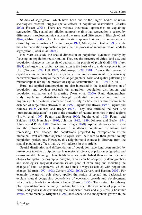
Here we use an actual data set to illustrate exploratory spatial data analysis (this

section) and spatial regression modeling (next section). The study concerns the

effect of highway expansion from 1980 to 1990 (the explanatory variable) on

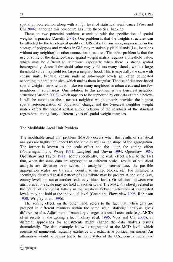
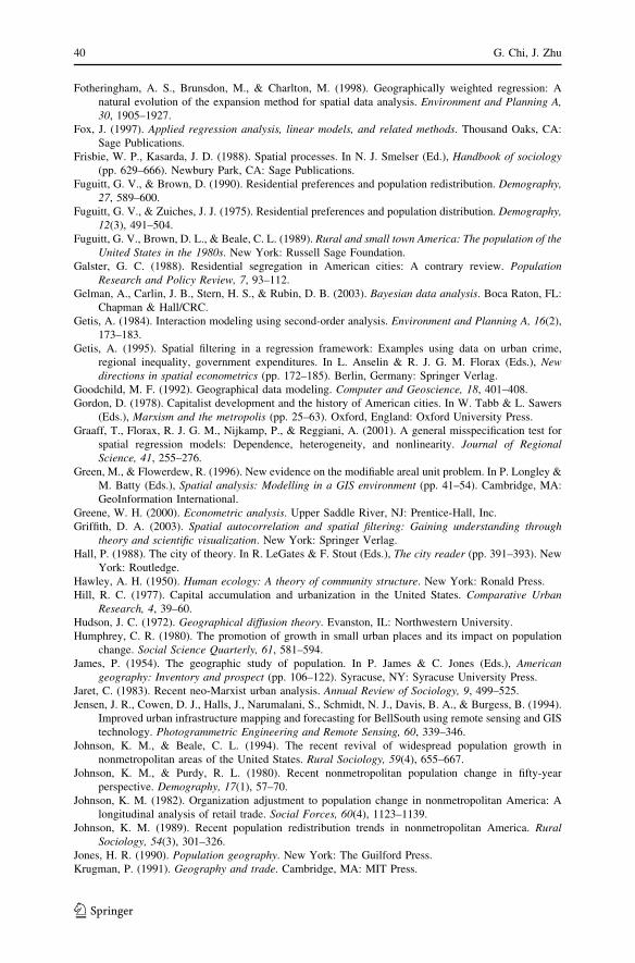
population change from 1990 to 2000 (the response variable; see the left panel of

Fig. 1) at the MCD level5 in Wisconsin. A review of the literature reveals that the

findings on the effects of highway construction on population change are sometimes

conflicting or equivocal, partly due to the different approaches taken for data

analysis (Chi et al. 2006). While some studies account for spatial autocorrelation,

others ignore it in the statistical models. These studies are also conducted at quite

different geographic scales ranging from communities, municipalities, counties, to

regions, and thus highway effects on population change may vary greatly at

different scales as a result of the MAUP. We argue that the MCD is an appropriate

scale to match the population-highway dynamics, because traffic analysis and

Fig. 1 The response variable and residuals of the standard regression

5 The boundaries, and even the names, of MCDs in Wisconsin are not fixed over time. Boundaries

change, new MCDs emerge, old MCDs disappear, names change, and status in the geographic hierarchy

shifts, e.g., towns become villages, villages become cities. In order to adjust the data for these changes,

we have set up three rules: new MCDs must be merged into the original MCDs from which they emerge;

disappearing MCD problems can be solved by dissolving the original MCDs into their current ‘‘home’’

MCDs; and occasionally, several distinct MCDs must be dissolved into one super-MCD in order to

establish a consistent data set over time. In the end, 1,837 MCD-like units (cities, villages, and towns)

constitute this analytical dataset.


123

forecast at the city, village, and town level is often necessary to transportation

planning.

In this section, we examine spatial autocorrelation of population change, which is

the response variable. In the next section, we examine the residuals after fitting a

regression model to assess how the incorporation of spatial autocorrelation in the

regression model affects the statistical analysis. A visual examination of the left

panel of Fig. 1 suggests that spatial autocorrelation of population change is

plausible and that the assumption of independent errors may not be appropriate in a

standard linear regression. But, at this point, we do not know whether the spatial

autocorrelation is statistically significant, and even if it is significant, we do not

know whether it can be ‘‘explained away’’ by the spatial autocorrelation in the

explanatory variables.

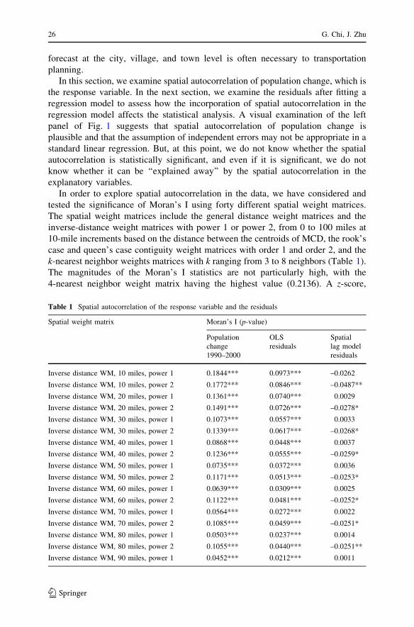
In order to explore spatial autocorrelation in the data, we have considered and

tested the significance of Moran’s I using forty different spatial weight matrices.

The spatial weight matrices include the general distance weight matrices and the

inverse-distance weight matrices with power 1 or power 2, from 0 to 100 miles at

10-mile increments based on the distance between the centroids of MCD, the rook’s

case and queen’s case contiguity weight matrices with order 1 and order 2, and the

k-nearest neighbor weights matrices with k ranging from 3 to 8 neighbors (Table 1).

The magnitudes of the Moran’s I statistics are not particularly high, with the

4-nearest neighbor weight matrix having the highest value (0.2136). A z-score,

Table 1 Spatial autocorrelation of the response variable and the residuals

Spatial weight matrix Moran’s I (p-value)

Population

change

1990–2000

OLS

residuals

Spatial

lag model

residuals

Inverse distance WM, 10 miles, power 1 0.1844*** 0.0973*** –0.0262

Inverse distance WM, 10 miles, power 2 0.1772*** 0.0846*** –0.0487**

Inverse distance WM, 20 miles, power 1 0.1361*** 0.0740*** 0.0029

Inverse distance WM, 20 miles, power 2 0.1491*** 0.0726*** –0.0278*














26 G. Chi, J. Zhu

123

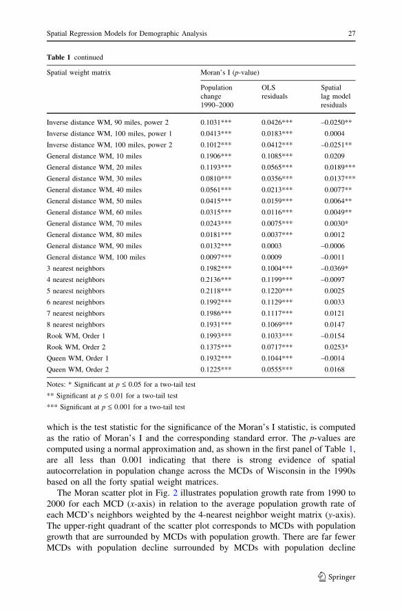
which is the test statistic for the significance of the Moran’s I statistic, is computed

as the ratio of Moran’s I and the corresponding standard error. The p-values are

computed using a normal approximation and, as shown in the first panel of Table 1,

are all less than 0.001 indicating that there is strong evidence of spatial

autocorrelation in population change across the MCDs of Wisconsin in the 1990s

based on all the forty spatial weight matrices.

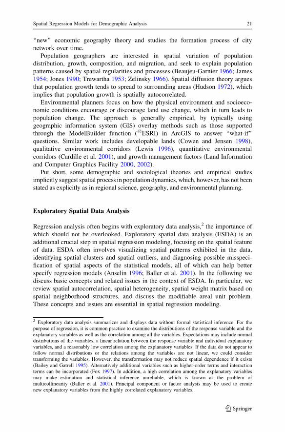
The Moran scatter plot in Fig. 2 illustrates population growth rate from 1990 to

2000 for each MCD (x-axis) in relation to the average population growth rate of

each MCD’s neighbors weighted by the 4-nearest neighbor weight matrix (y-axis).

The upper-right quadrant of the scatter plot corresponds to MCDs with population

growth that are surrounded by MCDs with population growth. There are far fewer

MCDs with population decline surrounded by MCDs with population decline

Table 1 continued

Spatial weight matrix Moran’s I (p-value)

Population

change

1990–2000

OLS

residuals

Spatial

lag model

residuals




General distance WM, 10 miles 0.1906*** 0.1085*** 0.0209

General distance WM, 20 miles 0.1193*** 0.0565*** 0.0189***

General distance WM, 30 miles 0.0810*** 0.0356*** 0.0137***

General distance WM, 40 miles 0.0561*** 0.0213*** 0.0077**



General distance WM, 70 miles 0.0243*** 0.0075*** 0.0030*

General distance WM, 80 miles 0.0181*** 0.0037*** 0.0012

General distance WM, 90 miles 0.0132*** 0.0003 –0.0006

General distance WM, 100 miles 0.0097*** 0.0009 –0.0011

3 nearest neighbors 0.1982*** 0.1004*** –0.0369*

4 nearest neighbors 0.2136*** 0.1199*** –0.0097

5 nearest neighbors 0.2118*** 0.1220*** 0.0025




Rook WM, Order 1 0.1993*** 0.1033*** –0.0154

Rook WM, Order 2 0.1375*** 0.0717*** 0.0253*

Queen WM, Order 1 0.1932*** 0.1044*** –0.0014

Queen WM, Order 2 0.1225*** 0.0555*** 0.0168

Notes: * Significant at p £ 0.05 for a two-tail test

** Significant at p £ 0.01 for a two-tail test

*** Significant at p £ 0.001 for a two-tail test


123

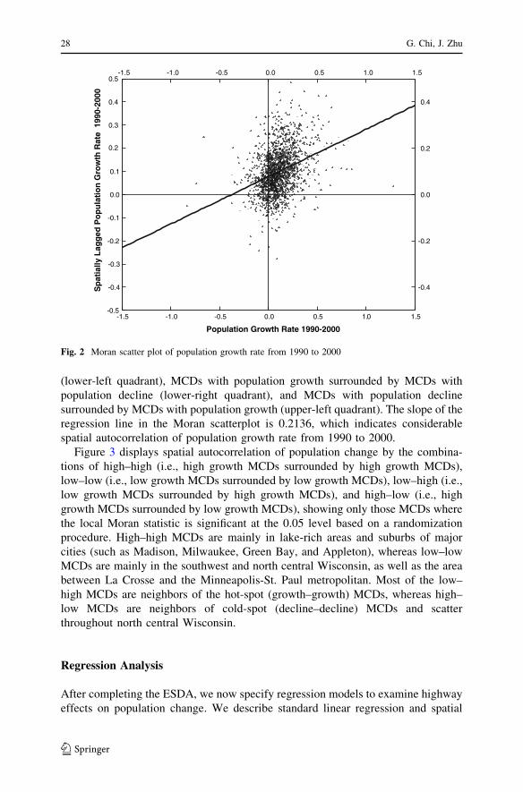
(lower-left quadrant), MCDs with population growth surrounded by MCDs with

population decline (lower-right quadrant), and MCDs with population decline

surrounded by MCDs with population growth (upper-left quadrant). The slope of the

regression line in the Moran scatterplot is 0.2136, which indicates considerable

spatial autocorrelation of population growth rate from 1990 to 2000.

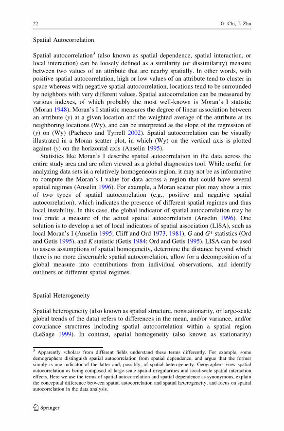
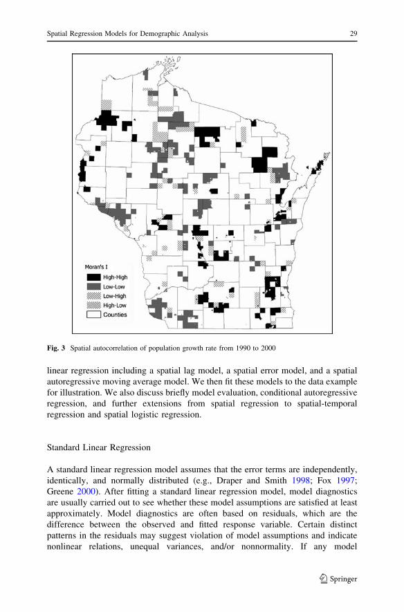
Figure 3 displays spatial autocorrelation of population change by the combina-

tions of high–high (i.e., high growth MCDs surrounded by high growth MCDs),

low–low (i.e., low growth MCDs surrounded by low growth MCDs), low–high (i.e.,

low growth MCDs surrounded by high growth MCDs), and high–low (i.e., high

growth MCDs surrounded by low growth MCDs), showing only those MCDs where

the local Moran statistic is significant at the 0.05 level based on a randomization

procedure. High–high MCDs are mainly in lake-rich areas and suburbs of major

cities (such as Madison, Milwaukee, Green Bay, and Appleton), whereas low–low

MCDs are mainly in the southwest and north central Wisconsin, as well as the area

between La Crosse and the Minneapolis-St. Paul metropolitan. Most of the low–

high MCDs are neighbors of the hot-spot (growth–growth) MCDs, whereas high–

low MCDs are neighbors of cold-spot (decline–decline) MCDs and scatter

throughout north central Wisconsin.

Regression Analysis

After completing the ESDA, we now specify regression models to examine highway

effects on population change. We describe standard linear regression and spatial

1.51.00.50.0-0.5-1.0-1.5

Population Growth Rate 1990-2000

1.51.00.50.0-0.5-1.0-1.50.5

0.4

0.3

0.2

0.1

0.0

-0.1

-0.2

-0.3

-0.4

-0.5

Sp

atia

lly L

agg

ed P

op

ula

tio

n G

row

th R

ate

199

0-20

00

0.4

0.2

0.0

-0.2

-0.4

Fig. 2 Moran scatter plot of population growth rate from 1990 to 2000

28 G. Chi, J. Zhu

123

linear regression including a spatial lag model, a spatial error model, and a spatial

autoregressive moving average model. We then fit these models to the data example

for illustration. We also discuss briefly model evaluation, conditional autoregressive

regression, and further extensions from spatial regression to spatial-temporal

regression and spatial logistic regression.

Standard Linear Regression

A standard linear regression model assumes that the error terms are independently,

identically, and normally distributed (e.g., Draper and Smith 1998; Fox 1997;

Greene 2000). After fitting a standard linear regression model, model diagnostics

are usually carried out to see whether these model assumptions are satisfied at least

approximately. Model diagnostics are often based on residuals, which are the

difference between the observed and fitted response variable. Certain distinct

patterns in the residuals may suggest violation of model assumptions and indicate

nonlinear relations, unequal variances, and/or nonnormality. If any model

Fig. 3 Spatial autocorrelation of population growth rate from 1990 to 2000


123

assumption is violated, standard linear regression may not be appropriate or

adequate and the subsequent statistical inference of model parameters may not be

reliable.

Here we are particularly interested in the independence assumption of the errors,

which is often violated in demographic studies due to spatial autocorrelation.

Possible diagnostic tools are Moran’s I plot,6 contour plot, and Moran’s I statistic of

the residuals (Baller et al. 2001; Loftin and Ward 1983). If there is spatial

autocorrelation in the errors, then standard linear regression fitting may yield

unreliable results. For example, standard errors of the regression coefficient

estimates tend to be underestimated or overestimated, giving rise to significant or

insignificant relations that may be otherwise (Baller et al. 2001; Doreian 1980;

Loftin and Ward 1983).

Spatial Linear Regression

Spatial linear regression models may be viewed as generalization of standard linear

regression models such that spatial autocorrelation is allowed and accounted for

explicitly by spatial models. The model parameters include the usual regression

coefficients of the explanatory variables (b) and the variance of the error term (r2).

In addition, the most commonly used spatial regression models have a spatial

autoregressive coefficient (q), which measures the strength of spatial autocorrela-

tion. A spatial weight matrix (W) corresponding to a neighborhood structure and a

variance weight matrix (D) are pre-specified. More complicated spatial models are

possible, but we restrict our attention to the spatial models with at most two spatial

autoregressive coefficients. Spatial linear regression models are usually fitted by

maximum likelihood (or equivalently generalized least squares for b) (Anselin

1988). Other approaches are possible including spatial filtering (Getis 1995; Griffith

2003) and geographically weighted regression focusing on the specification of

spatial heterogeneity (Fotheringham et al. 1998).

Spatial Lag Model, Spatial Error Model, and Spatial Autoregressive Moving

Average Model

Now, we consider specific spatial linear regression models that vary in the way

spatial models for the error terms are specified. Two popular spatial regression

models are the spatial error model and the spatial lag model. A spatial lag model is

specified as:

6 The Moran’s I plot of errors can also detect if there are any outliers. Outliers are not necessarily ‘‘bad,’’

and further exploration of the outliers might provide interesting findings. Practically, we can use the

outliers as one independent variable where the outliers are represented as 1 while others as 0. If these

outliers are ‘‘real’’ outliers, the coefficient should be statistically significant. In the spatial data analysis,

outliers detected by Moran scatter plot may indicate possible problems with the specification of the spatial

weights matrix or with the spatial scale at which the observations are recorded (Anselin 1996). Outliers

should be studied carefully before being discarded.

30 G. Chi, J. Zhu

123

Y ¼ Xb þ qWY þ e; ð1Þ

where Y denotes the vector of response variables, X denotes the matrix of explan-

atory variables, W denotes the spatial weight matrix, and e denotes the vector of

error terms that are independent but not necessarily identically distributed. In

contrast, a spatial error model is specified as:

Y ¼ Xb þ u; u ¼ qWu þ e; ð2Þ

where the terms are defined in the same way as the spatial lag model.

For spatial lag models, spatial autocorrelation is modeled by a linear relation

between the response variable (y) and the associated spatially lagged variable (Wy),

but for spatial error models, spatial autocorrelation is modeled by an error term (u)

and the associated spatially lagged error term (Wu) (Anselin and Bera 1998). In

either case, interpretation of a significant spatial autoregressive coefficient is not

always straightforward. A significant spatial lag term may indicate strong spatial

dependence, but may also indicate a mismatch of spatial scales between the

phenomenon under study and at which it is measured as a result of the MAUP. A

significant spatial error term indicates spatial autocorrelation in errors, which may

be due to key explanatory variables that are not included in the model.

However, the taxonomy of spatial lag model and spatial error model may be

overly simplistic and may exclude other possible spatial autocorrelation mecha-

nisms, such as the existence of both lag and error autocorrelations (Anselin 1988,

2003). A spatial autoregressive moving average (SARMA) model can be

constructed to include both the spatial lag and spatial error models. A simple

version of the SARMA specification combines a first-order spatial lag model with a

first-order spatial error model and can be expressed as a combination of (1) and (2):

Y ¼ q1W1Y þ Xb þ u; u ¼ q2W2u þ e: ð3Þ

With some algebraic manipulation, (3) can be rewritten as:

Y ¼ q1W1Y þ q2W2Y � q1q2W2W1Y þ Xb � q2W2Xh þ e: ð4Þ

In practice, we can treat a spatially weighted response variable as an additional

explanatory variable when fitting model (4). A test for lack of spatial autocorrelation

can be conducted, although the test does not provide any specific guidance

regarding the exact nature of autocorrelation when the null hypothesis is rejected

(Anselin and Bera 1998).

Model Evaluation

For model assessment and comparison, there are at least two approaches addressed

in current literature. One is a data-driven approach, which tests for lack of spatial

error autocorrelation after fitting a spatial lag model, and then tests for lack of

spatial lag autocorrelation after fitting a spatial error model. In a study examining

population growth, Voss and Chi (2006) find that the data-driven approach can help


123

determine which specification is the better model for accounting for the spatial

autocorrelation. The other is a theory-based approach, which suggests that the

choice between the spatial lag model and the spatial error model should be based on

substantive grounds (Doreian 1980). While both approaches are used in spatial

regression, the data-driven method is often preferred, because often it is the data

rather than formal theoretical concerns that motivate spatial data analysis (Anselin

2002, 2003).

For a given data set, various linear regression models can be specified.

Likelihood ratio tests (LRT) can be performed to compare models that are nested

(i.e., one simpler model can be reduced from the other more complex model by

constraining certain parameters in the complex model). If two models are not

nested, Akaike’s Information Criterion (AIC) and Schwartz’s Bayesian Information

Criterion (BIC) are often used, which measure the fit of the model to the data but

penalize models that are overly complex. Models having a smaller AIC or a smaller

BIC are considered the better models in the sense of model fitting balanced with

model parsimony. In addition, several other tests are useful for model diagnostics.

For example, heteroscedasticity can be detected by the Breusch-Pagan test and the

spatial Breusch-Pagan test, while goodness-of-fit (GOF) of the models can be

detected by the Lagrange Multiplier (LM) test. A test for nonlinearity appears to be

useful for detecting anisotropy and nonstationarity (Bailey and Gatrell 1995; Graaff

et al. 2001).

CAR Models

Spatial error models and sometimes spatial lag models are referred to as the

simultaneous autoregressive model (SAR). Another popular class of models is the

conditional autoregressive (CAR) models. The key distinction between the SAR and

the CAR models is in the model specification (Cressie 1993). SAR models explain

the relations among response variables at all locations on the lattice simultaneously

and the spatial effect is considered to be endogenous. In contrast, CAR models

specify the distribution of a response variable at one location by conditioning on the

values of its neighbors in the neighborhood and the spatial effect of the neighbors is

considered to be exogenous (Anselin 2003). While CAR models are popular in the

statistics literature and many other disciplines, SAR models are favored in spatial

econometrics and spatial demography, possibly because interpretation of the spatial

autocorrelation coefficient resembles that of standard linear regression and thus may

seem more natural. The relation between the two types of models is close, however,

as SAR models (from a spatial error model) may be represented by possibly higher

order CAR models (Cressie 1993).

Spatial-temporal Regression

The spatial regression models considered so far account for spatial autocorrelation

within a same time period but not across different time periods, as all the variables

32 G. Chi, J. Zhu

123

in (1) to (4) refer to a given cross-sectional point in time. Nevertheless, for all

variables, we can add their corresponding time-lagged variables to establish a

spatial-temporal regression model, which captures both the spatial and the temporal

autocorrelation (Elhorst 2001). For example, we may extend model (2) to:

Yt ¼ Xtbþ qWYt � qWXtbþ s1Yt�1 þ Xt�1s2 þ s3WYt�1 þWXt�1s4 þ e: ð5Þ

The spatial-temporal regression model in (5) provides a practical way for

forecasting, if we consider only the time-lagged explanatory variables. That is, by

removing explanatory variables from the same time point as the base year of

forecasting, we obtain a spatial-temporal regression model suitable for forecasting

such as follow:

Yt ¼ s1Yt�1 þ Xt�1s2 þ s3WYt�1 þWXt�1s4 þ e: ð6Þ

Spatial Logistic Regression

In the above models, the response variables are continuous and are assumed to

follow normal distributions. When the response variables are binary (0 or 1),

logistic regression would be more suitable. However, to account for spatial

autocorrelation, spatial logistic regression models would be more appropriate. A

number of approaches have been proposed, such as autologistic regression

models (Anselin 2002; Besag 1974), marginal models fitted by generalized

estimating equations (GEE) (Diggle et al. 2002), and generalized linear mixed

models (GLMM) (Littell et al. 2006). With autologistic regression models and

GLMM, it is becoming increasingly popular to employ the Markov Chain Monte

Carlo (MCMC) approach, a powerful statistical computing technique, for

statistical inference (Banerjee et al. 2003; Fleming 2004; Gelman et al. 2003).

In Zhu et al. (2005), spatial autologistic regression models are extended to a

class of spatial-temporal autologistic regression models for the analysis of

spatial-temporal binary data.

Data Example

For illustration, we fit both standard regression model and various spatial regression

models to the population change data example here. We first describe the response

variable and the explanatory variables. We then fit a standard linear regression to the

data and perform model diagnostics to check the model assumptions. Afterwards,

we fit a spatial lag model, a spatial error model, and a SARMA model to the data

and again perform model diagnostics. Finally we assess and compare these various

models using the aforementioned techniques.

The response variable here is a rate of population growth, expressed as the

natural log of the ratio of the 2000 census population over the 1990 census


123

population. The explanatory variables are four dummy variables indicating MCDs

within 10 miles of highway expansion in 1980–1985, within 10–20 miles from

highway expansion in 1980–1985, within 10 miles of highway expansion in 1985–

1990, and within 10–20 miles from highway expansion in 1985–1990, respectively.

If a MCD fits into a distance buffer category, it is coded as 1; 0 otherwise. We also

attempt to include other explanatory variables, as many variables are potentially

related to population changes and omitting relevant explanatory variables may give

rise to various problems (Dalenberg and Partridge 1997). However, many of these

variables may be highly correlated, which is known as multicollinearity. To solve

the dilemma, we use principal component analysis and the ModelBuilder function

of ArcGIS to generate five indices, namely demographic characteristics, social and

economic conditions, transportation accessibility, natural amenities, and land

conversion and development in 1990, from 37 key factors of population change.7 In

total, we have six additional explanatory variables (which we will call controlled

variables) including these five indices as well as the rate of population growth from

1980 to 1990.

We now regress the response variable of population change from 1990 to 2000 on

the explanatory variables of highway expansion plus the six controlled variables

(the first panel of Table 2). The results from fitting a standard linear regression

model indicate that highway expansion finished 5–9 years before the population

change period has no significant effect on population change, whereas highway

expansion finished just before the population change period has a significant

positive impact on population change, for MCDs within 10 miles and 10–20 miles

from the segments of highway expansion.

The Moran’s I test on the residuals after fitting the standard linear regression

suggests that there is strong evidence of spatial autocorrelation among the residuals

(Moran’s I = 0.122; p-value \ 0.001). Thus the independence assumption of the

error term appears to be violated and we proceed to fit spatial linear regression

models in order to account for the spatial autocorrelation.

In particular, we use a spatial lag model, a spatial error model, and a SARMA

model to reanalyze the data. For the spatial weight matrix, we select the 4-nearest

neighbor weight matrix, which provides the highest spatial autocorrelation of the

response variable (the left panel of Table 1), for the spatial lag model. For the

spatial error model, we select the 5-nearest neighbor weight matrix, which provides

the highest spatial autocorrelation of the residuals (the middle panel of Table 1).

The SARMA model has both a spatial lag term and a spatial error term. Thus we use

7 An extensive review of the relevant literature results in more than 37 variables that significantly affect

population change theoretically or empirically (Chi 2006). These 37 variables are chosen for this research

on the basis of a combination of judgment established theoretical or empirical relationships, and the

availability of data. The variables that have been used to generate the demographic index are population

density, age structure, race, college population, educational attainment, stayers, female-headed

households, and seasonal housing. Social and economic conditions include crime rate, school

performance, employment, income, public transportation, public water, new housing, buses, county seat

status, and real estate value. Transportation accessibility is made up of residential preference,

accessibility to airports and highway, highway infrastructure, and journey to work. Natural amenities

contain forest, water, the lengths of lakeshore, riverbank, and coastline, golf courses, and slope. Land

development and conversion include water, wetlands, slope, tax-exempt lands, and built-up lands.

34 G. Chi, J. Zhu

123

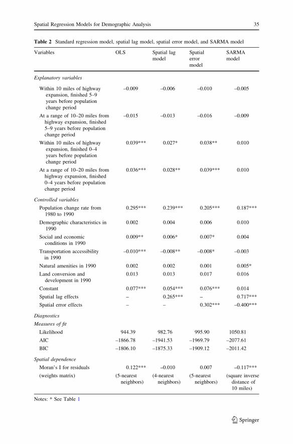
Table 2 Standard regression model, spatial lag model, spatial error model, and SARMA model

Variables OLS Spatial lag

model

Spatial

error

model

SARMA

model

Explanatory variables

Within 10 miles of highway

expansion, finished 5–9

years before population

change period

–0.009 –0.006 –0.010 –0.005

At a range of 10–20 miles from

highway expansion, finished

5–9 years before population

change period

–0.015 –0.013 –0.016 –0.009

Within 10 miles of highway

expansion, finished 0–4

years before population

change period

0.039*** 0.027* 0.038** 0.010

At a range of 10–20 miles from

highway expansion, finished

0–4 years before population

change period

0.036*** 0.028** 0.039*** 0.010

Controlled variables

Population change rate from

1980 to 1990

0.295*** 0.239*** 0.205*** 0.187***

Demographic characteristics in

1990

0.002 0.004 0.006 0.010

Social and economic

conditions in 1990

0.009** 0.006* 0.007* 0.004

Transportation accessibility

in 1990

–0.010*** –0.008** –0.008* –0.003

Natural amenities in 1990 0.002 0.002 0.001 0.005*

Land conversion and

development in 1990

0.013 0.013 0.017 0.016

Constant 0.077*** 0.054*** 0.076*** 0.014

Spatial lag effects – 0.265*** – 0.717***

Spatial error effects – – 0.302*** –0.400***

Diagnostics

Measures of fit

Likelihood 944.39 982.76 995.90 1050.81

AIC –1866.78 –1941.53 –1969.79 –2077.61

BIC –1806.10 –1875.33 –1909.12 –2011.42

Spatial dependence

Moran’s I for residuals 0.122*** –0.010 0.007 –0.117***

(weights matrix) (5-nearest

neighbors)

(4-nearest

neighbors)

(5-nearest

neighbors)

(square inverse

distance of

10 miles)

Notes: * See Table 1


123

the 4-nearest neighbor weight matrix for the spatial lag term, and select the squared

inverse distance within 10 miles for the spatial error term, as it provides the highest

spatial autocorrelation of the residuals after fitting a spatial lag model (the right

panel of Table 1).

Table 2 summarizes the results from fitting three spatial regression models in

addition to standard linear regression. Recall that, in standard linear regression,

highway expansion finished just before the population change period for MCDs

within 10 miles and 10–20 miles from the segments of highway expansion are both

significant. These two explanatory variables remain significant in the spatial lag

model and spatial error model, although the regression coefficients are smaller in

magnitude and the p-value is not as small. In the SARMA model, however, these

two explanatory variables are no longer significant.

Moreover, all the three spatial linear regression models appear to be better fit

than the standard linear regression, based on the fact that the AIC and BIC values

are smaller for the spatial regression models. Between the spatial error model and

the spatial lag model, the former may be preferred, because of slightly smaller AIC

and BIC values. Of all the three spatial regression models, the SARMA model has

clear advantage over the spatial lag and spatial error models, judging again from the

AIC and BIC values. All the spatial autocorrelation coefficients are significant in the

three spatial linear regression models.

The residuals from the spatial lag and spatial error models do not exhibit spatial

autocorrelation, but the residuals from the SARMA model have significant spatial

autocorrelation, all with respect to the corresponding spatial weight matrix.

Although the SARMA model has a better fit than the other two spatial models, the

remaining spatial autocorrelation in its residuals casts slight doubt about the

adequacy of the model. One possible remedy would be to consider other spatial

weight matrices and/or somewhat more complex spatial models to account for the

additional spatial autocorrelation. In future research, all forty spatial weight

matrices can be applied to the four regression models. According to each spatial

weight matrix, one set of the AIC and BIC values and the spatial autocorrelation of

residuals will be examined for each model, as it may be fairer to compare the four

regression models based on the same spatial weight matrix. AIC and BIC may also

help select the optimal spatial weight matrix within and across different regression

models, although the legitimacy of such an approach needs to be further established.

The scale effect may have played a role in this example because the five

controlled variables influence population change at different scales but are still

examined only at the MCD level. For example, natural amenities tend to attract

migrants at the regional level and thus, even though the natural amenity index is

expected to have important effects on population change, the analysis gives opposite

results (Table 2). To mitigate the scale effect, we could consider constructing a

hierarchical model at various spatial scales (e.g., from regional, local, household,

down to individual levels). Possible approaches are a two-stage procedure (Sampson

et al. 1999), a Bayesian hierarchical modeling approach (Parent and Riou 2005),

and simultaneous estimation of spatial dependence within a hierarchical context

(Chi and Voss 2005), although analysis can be challenging due to lack of suitable

data and limitation of software support.

36 G. Chi, J. Zhu

123

Discussion

Spatial demographic analysis is emerging as an important and interesting topic for

demographers to explore, as evidenced by an increasing number of publications and

conference presentations that apply spatial econometrics and analysis techniques for

demographic studies. In this article, spatial theories of population dynamics are

summarized, and spatial regression models and the associated basic concepts and

issues are discussed through an illustration of highway effects on population change

in the 1990s at the MCD level in Wisconsin.

Despite its complexity, spatial demographic analysis has in recent years become

more accessible for demographers to explore, due to the upsurge in the availability

of geographically referenced data, the development of user-friendly spatial data

analysis software packages, and the computing power combined with affordable

computers. Three types of demographic products are especially useful for spatial

demographic analysis: the topologically integrated geographic encoding and

reference (TIGER) system products, census summary files of 1980, 1990, and

2000, and the sociological and demographic survey database when companioned

with the geocoding technique. Related geophysical information from rich GIS data

sources and remote sensing images are often useful for demographic studies and can

be easily added into the geographically referenced demographic database. In

addition, the last decade has seen rapid development of spatial statistical software

packages including GeoDa, SpaceStat, R, S-plus, GWR, and others. Extensions

have also been developed for spatial statistical analysis in traditional software such

as SAS, SPSS, Stata, and others. GIS software also has powerful functions of spatial

statistics. Moreover, the increasing computing power facilitated in inexpensive

computers makes it affordable for demographers to conduct spatial demographic

analysis. Furthermore, recent years have seen a dramatically growing number of

textbooks, journal articles, and conference presentations advancing or using spatial

data analysis (Florax and Van der Vlist 2003), which creates abundant opportunities

for demographers to study this technique.

Looking forward, spatial demography may advance in two perspectives. First,

explicitly spatial demographic theories may be proposed. There are some

demographic and sociological theories and empirical studies suggesting spatial

effects in population dynamics as discussed in the section of spatial demographic

theories. Nevertheless, spatial effects have not yet been explicitly stated in current

demographic theories. It is obvious that advances in spatial techniques and

availability of spatial data are allowing us to ask new demographic questions and

develop new demographic theories. The field of demography can borrow the strong

spatial components from the spatially explicit theories in geography and regional

science to strengthen itself.

Second, besides spatial regression models, other spatial analysis techniques may

be applicable to demographic studies. Spatial point data analysis, which has been

used widely in diverse disciplines such as epidemiology and forestry, could become

a potentially useful technique for formal demographic studies, especially with the

development of geocoding techniques and individual demographic survey database.

Geostatistics, which has been applied frequently in physical and biological sciences,


123

can be used potentially as an interpolation technique for demographic estimation.

Spatial interaction modeling, which becomes a fourth type of spatial data analysis

techniques, can be very useful for studying migration and demographic network. Put

short, numerous spatial data analysis methods are available in other fields and can

be well employed for demographic studies.

We believe that spatial demography is moving to a new and exciting stage along

with the rapid advances in spatial analysis techniques and the increasing availability

of geographically referenced data. The time appears to be ripe for demographers to

explore and enrich the field of spatial demography.

Acknowledgments We are indebted to Paul R. Voss for his guidance with this research and forproviding us with insightful suggestions on earlier drafts. Appreciation is extended to three anonymousreviewers for their many helpful comments. We also acknowledge support from the Social ScienceResearch Center at Mississippi State University and Department of Statistics and Department of SoilScience at University of Wisconsin-Madison. Funding has been provided for this research by the USDACooperative State Research, Education and Extension Service (CSREES) Hatch project WIS04536 andthe Wisconsin Alumni Research Foundation.

References

Alba, R. D., & Logan, J. R. (1993). Minority proximity to whites in suburbs: An individual-level analysis

of segregation. American Journal of Sociology, 98(6), 1388–1427.

Anselin, L. (1988). Spatial econometrics: Methods and models. Dordrecht, Netherlands: Kluwer

Academic Publishers.

Anselin, L. (1990). Spatial dependence and spatial structural instability in applied regression analysis.

Journal of Regional Science, 30, 185–207.

Anselin, L. (1992). SpaceStat tutorial: A workbook for using SpaceStat in the analysis of spatial data.

National Center for Geographic Information and Analysis, University of California, Santa Barbara

CA.

Anselin, L. (1995). Local indicators of spatial autocorrelation—LISA. Geographical Analysis, 27, 93–

115.

Anselin, L. (1996). The Moran scatterplot as an ESDA tool to assess local instability in spatial

association. In M. Fischer, H. J. Scholten, & D. Unwin (Eds.), Spatial analytical perspectives on GIS(pp. 111–125). London, England: Taylor & Francis.

Anselin, L. (2001). Spatial econometrics. In B. Baltagi (Ed.), A companion to theoretical econometrics(pp. 310–330). Oxford, England: Blackwell.

Anselin, L. (2002). Under the hood: Issues in the specification and interpretation of spatial regression

models. Agricultural Economics, 27, 247–267.

Anselin, L. (2003). Spatial externalities, spatial multipliers, and spatial econometrics. InternationalRegional Science Review, 26, 153–166.

Anselin, L., & Griffith, D. A. (1988). Do spatial effects really matter in regression analysis? Papers inRegional Science, 65, 11–34.

Anselin, L., & Bera, A. (1998). Spatial dependence in linear regression models with an introduction to

spatial econometrics. In A. Ullah & D. Giles (Eds.), Handbook of applied economic statistics (pp.

237–289). New York: Marcel Dekker.

Bailey, T. C., & Gatrell, A. C. (1995). Interactive spatial data analysis. Harlow, England: Longman

Scientific & Technical.

Baller, R. D., Anselin, L., Messner, S. F., Deane, G., & Hawkins, D. F. (2001). Structural covariates of

U. S. county homicide rates: Incorporating spatial effects. Criminology, 39, 561–590.

Banerjee, S., Carlin, B. P., & Gelfand, A. E. (2003). Hierarchical modeling and analysis for spatial data.

Boca Raton, FL: Chapman & Hall/CRC.

Beaujeu-Garnier, J. (1966). Geography of population. London, England: Longman.

Berry, B. J. L., & Kasarda, J. D. (1977). Contemporary urban ecology. New York: Macmillan.

38 G. Chi, J. Zhu

123

Besag, J. (1974). Spatial interaction and the statistical analysis of lattice systems. Journal of the RoyalStatistical Society, Series B, 36, 192–236.

Boarnet, M. G. (1997). Highways and economic productivity: Interpreting recent evidence. Journal ofPlanning Literature, 11(4), 476–486.

Boarnet, M. G. (1998). Spillovers and the locational effects of public infrastructure. Journal of RegionalScience, 38(3), 381–400.

Brown, D. L., Fuguitt, G. V., Heaton, T. B., & Waseem, S. (1997). Continuities in size of place

preferences in the United States, 1972–1992. Rural Sociology, 62(4), 408–428.

Cardille, J. A., Ventura, S. J., & Turner, M. G. (2001). Environmental and social factors influencing

wildfires in the Upper Midwest, USA. Ecological Applications, 11, 111–127.

Case, A., Rosen, H. S., & Hines, J. R. (1993). Budget spillovers and fiscal policy interdependence:

Evidence from the states. Journal of Public Economics, 52, 285–307.

Cervero, R. (2002). Induced travel demand: Research design, empirical evidence, and normative policies.

Journal of Planning Literature, 17(1), 3–20.

Cervero, R. (2003). Road expansion, urban growth, and induced travel: A path analysis. Journal of theAmerican Planning Association, 69(2), 145–163.

Cervero, R., & Hansen, M. (2002). Induced travel demand and induced road investment: A simultaneous-

equation analysis. Journal of Transport Economics and Policy, 36(3), 469–490.

Charles, C. Z. (2003). The dynamics of racial residential segregation. Annual Review of Sociology, 29,

167–207.

Chi, G. (2006). Environmental demography, small-area population forecasting, and spatio-temporaleconometric modeling: Demographics, accessibility, developability, desirability, and livability.

Dissertation, Department of Urban and Regional Planning, University of Wisconsin-Madison,

Madison WI.

Chi, G., & Voss, P. R. (2005). Migration decision-making: A hierarchical regression approach. Journal ofRegional Analysis and Policy, 35(2), 11–22.

Chi, G., Voss, P. R., & Deller, S. C. (2006). Rethinking highway effects on population change. PublicWorks Management and Policy, 11, 18–32.

Christaller, W. (1966). Central places in southern Germany (Die zentralen Orte in Suddeutschland,

Baskin CW, 1933, Trans). Englewood Cliffs, NJ: Prentice-Hall.

Clark, W. (1996). Understanding residential segregation in American cities: Interpreting the evidence.

Population Research and Policy Review, 5, 95–127.

Cliff, A., & Ord, J. K. (1973). Spatial autocorrelation. London, England: Pion Limited.

Cliff, A., & Ord, J. K. (1981). Spatial processes, models and applications. London, England: Pion

Limited.

Cowen, D. J., & Jensen, J. R. (1998). Extraction and modeling of urban attributes using remote sensing

technology. In D. Liverman, E. F. Moran, R. R. Rindfuss, & P. C. Stern (Eds.), People and pixels:Linking remote sensing and social science (pp. 164–188). Washington, DC: National Academy

Press.

Cressie, N. (1993). Statistics for spatial data. New York: Wiley.

Dalenberg, D. R., & Partridge, M. D. (1997). Public infrastructure and wages: Public capital’s role as a

productive input and household amenity. Land Economics, 73, 268–284.

Diggle, P., Heagerty, P., Liang, K. Y., & Zeger, S. (2002). Analysis of longitudinal data. Oxford,

England: Oxford University Press.

Doreian, P. (1980). Linear models with spatial distributed data: Spatial disturbances or spatial effects?

Sociological Methods and Research, 9, 29–60.

Draper, N. R., & Smith, H. (1998). Applied regression analysis. New York: John Wiley & Sons.

Elhorst, P. J. (2001). Dynamic models in space and time. Geographical Analysis, 33, 119–140.

Fleming, M. M. (2004). Techniques for estimating spatially dependent discrete choice models. In L.

Anselin, R. J. G. M. Florax, & S. J. Rey (Eds.), Advances in spatial econometrics (pp. 145–168).

Berlin, Germany: Springer.

Florax, R. J. G. M., & Van der Vlist, A. J. (2003). Spatial econometric data analysis: Moving beyond

traditional models. International Regional Science Review, 26(3), 223–243.

Fossett, M. (2005). Urban and spatial demography. In D. L. Poston, & M. Micklin (Eds.), Handbook ofPopulation (pp. 479–524). New York: Springer.

Fotheringham, A. S., & Wong, D. W. S. (1991). The modifiable areal unit problem in multivariate

statistical analysis. Environment and Planning A, 23, 1025–1034.


123

Fotheringham, A. S., Brunsdon, M., & Charlton, M. (1998). Geographically weighted regression: A

natural evolution of the expansion method for spatial data analysis. Environment and Planning A,30, 1905–1927.

Fox, J. (1997). Applied regression analysis, linear models, and related methods. Thousand Oaks, CA:

Sage Publications.

Frisbie, W. P., Kasarda, J. D. (1988). Spatial processes. In N. J. Smelser (Ed.), Handbook of sociology(pp. 629–666). Newbury Park, CA: Sage Publications.

Fuguitt, G. V., & Brown, D. (1990). Residential preferences and population redistribution. Demography,27, 589–600.

Fuguitt, G. V., & Zuiches, J. J. (1975). Residential preferences and population distribution. Demography,12(3), 491–504.

Fuguitt, G. V., Brown, D. L., & Beale, C. L. (1989). Rural and small town America: The population of theUnited States in the 1980s. New York: Russell Sage Foundation.

Galster, G. C. (1988). Residential segregation in American cities: A contrary review. PopulationResearch and Policy Review, 7, 93–112.

Gelman, A., Carlin, J. B., Stern, H. S., & Rubin, D. B. (2003). Bayesian data analysis. Boca Raton, FL:

Chapman & Hall/CRC.

Getis, A. (1984). Interaction modeling using second-order analysis. Environment and Planning A, 16(2),

173–183.

Getis, A. (1995). Spatial filtering in a regression framework: Examples using data on urban crime,

regional inequality, government expenditures. In L. Anselin & R. J. G. M. Florax (Eds.), Newdirections in spatial econometrics (pp. 172–185). Berlin, Germany: Springer Verlag.

Goodchild, M. F. (1992). Geographical data modeling. Computer and Geoscience, 18, 401–408.

Gordon, D. (1978). Capitalist development and the history of American cities. In W. Tabb & L. Sawers

(Eds.), Marxism and the metropolis (pp. 25–63). Oxford, England: Oxford University Press.

Graaff, T., Florax, R. J. G. M., Nijkamp, P., & Reggiani, A. (2001). A general misspecification test for

spatial regression models: Dependence, heterogeneity, and nonlinearity. Journal of RegionalScience, 41, 255–276.

Green, M., & Flowerdew, R. (1996). New evidence on the modifiable areal unit problem. In P. Longley &

M. Batty (Eds.), Spatial analysis: Modelling in a GIS environment (pp. 41–54). Cambridge, MA:

GeoInformation International.

Greene, W. H. (2000). Econometric analysis. Upper Saddle River, NJ: Prentice-Hall, Inc.

Griffith, D. A. (2003). Spatial autocorrelation and spatial filtering: Gaining understanding throughtheory and scientific visualization. New York: Springer Verlag.

Hall, P. (1988). The city of theory. In R. LeGates & F. Stout (Eds.), The city reader (pp. 391–393). New

York: Routledge.

Hawley, A. H. (1950). Human ecology: A theory of community structure. New York: Ronald Press.

Hill, R. C. (1977). Capital accumulation and urbanization in the United States. Comparative UrbanResearch, 4, 39–60.

Hudson, J. C. (1972). Geographical diffusion theory. Evanston, IL: Northwestern University.

Humphrey, C. R. (1980). The promotion of growth in small urban places and its impact on population

change. Social Science Quarterly, 61, 581–594.

James, P. (1954). The geographic study of population. In P. James & C. Jones (Eds.), Americangeography: Inventory and prospect (pp. 106–122). Syracuse, NY: Syracuse University Press.

Jaret, C. (1983). Recent neo-Marxist urban analysis. Annual Review of Sociology, 9, 499–525.

Jensen, J. R., Cowen, D. J., Halls, J., Narumalani, S., Schmidt, N. J., Davis, B. A., & Burgess, B. (1994).

Improved urban infrastructure mapping and forecasting for BellSouth using remote sensing and GIS

technology. Photogrammetric Engineering and Remote Sensing, 60, 339–346.

Johnson, K. M., & Beale, C. L. (1994). The recent revival of widespread population growth in

nonmetropolitan areas of the United States. Rural Sociology, 59(4), 655–667.

Johnson, K. M., & Purdy, R. L. (1980). Recent nonmetropolitan population change in fifty-year

perspective. Demography, 17(1), 57–70.

Johnson, K. M. (1982). Organization adjustment to population change in nonmetropolitan America: A

longitudinal analysis of retail trade. Social Forces, 60(4), 1123–1139.

Johnson, K. M. (1989). Recent population redistribution trends in nonmetropolitan America. RuralSociology, 54(3), 301–326.

Jones, H. R. (1990). Population geography. New York: The Guilford Press.

Krugman, P. (1991). Geography and trade. Cambridge, MA: MIT Press.

40 G. Chi, J. Zhu

123

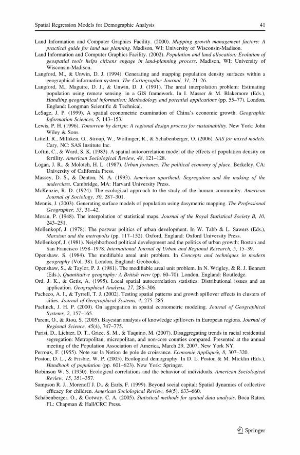
Land Information and Computer Graphics Facility. (2000). Mapping growth management factors: Apractical guide for land use planning. Madison, WI: University of Wisconsin-Madison.

Land Information and Computer Graphics Facility. (2002). Population and land allocation: Evolution ofgeospatial tools helps citizens engage in land-planning process. Madison, WI: University of

Wisconsin-Madison.

Langford, M., & Unwin, D. J. (1994). Generating and mapping population density surfaces within a

geographical information system. The Cartographic Journal, 31, 21–26.

Langford, M., Maguire, D. J., & Unwin, D. J. (1991). The areal interpolation problem: Estimating

population using remote sensing. in a GIS framework. In I. Masser & M. Blakemore (Eds.),

Handling geographical information: Methodology and potential applications (pp. 55–77). London,

England: Longman Scientific & Technical.

LeSage, J. P. (1999). A spatial econometric examination of China’s economic growth. GeographicInformation Sciences, 5, 143–153.

Lewis, P. H. (1996). Tomorrow by design: A regional design process for sustainability. New York: John

Wiley & Sons.

Littell, R., Milliken, G., Stroup, W., Wolfinger, R., & Schabenberger, O. (2006). SAS for mixed models.

Cary, NC: SAS Institute Inc.

Loftin, C., & Ward, S. K. (1983). A spatial autocorrelation model of the effects of population density on

fertility. American Sociological Review, 48, 121–128.

Logan, J. R., & Molotch, H. L. (1987). Urban fortunes: The political economy of place. Berkeley, CA:

University of California Press.

Massey, D. S., & Denton, N. A. (1993). American apartheid: Segregation and the making of theunderclass. Cambridge, MA: Harvard University Press.

McKenzie, R. D. (1924). The ecological approach to the study of the human community. AmericanJournal of Sociology, 30, 287–301.

Mennis, J. (2003). Generating surface models of population using dasymetric mapping. The ProfessionalGeographer, 55, 31–42.

Moran, P. (1948). The interpolation of statistical maps. Journal of the Royal Statistical Society B, 10,

243–251.

Mollenkopf, J. (1978). The postwar politics of urban development. In W. Tabb & L. Sawers (Eds.),

Marxism and the metropolis (pp. 117–152). Oxford, England: Oxford University Press.

Mollenkopf, J. (1981). Neighborhood political development and the politics of urban growth: Boston and

San Francisco 1958–1978. International Journal of Urban and Regional Research, 5, 15–39.

Openshaw. S. (1984). The modifiable areal unit problem. In Concepts and techniques in moderngeography (Vol. 38). London, England: Geobooks.

Openshaw, S., & Taylor, P. J. (1981). The modifiable areal unit problem. In N. Wrigley, & R. J. Bennett

(Eds.), Quantitative geography: A British view (pp. 60–70). London, England: Routledge.

Ord, J. K., & Getis, A. (1995). Local spatial autocorrelation statistics: Distributional issues and an

application. Geographical Analysis, 27, 286–306.

Pacheco, A. I., & Tyrrell, T. J. (2002). Testing spatial patterns and growth spillover effects in clusters of

cities. Journal of Geographical Systems, 4, 275–285.

Paelinck, J. H. P. (2000). On aggregation in spatial econometric modeling. Journal of GeographicalSystems, 2, 157–165.

Parent, O., & Riou, S. (2005). Bayesian analysis of knowledge spillovers in European regions. Journal ofRegional Science, 45(4), 747–775.

Parisi, D., Lichter, D. T., Grice, S. M., & Taquino, M. (2007). Disaggregating trends in racial residential

segregation: Metropolitan, micropolitan, and non-core counties compared. Presented at the annual

meeting of the Population Association of America, March 29, 2007, New York NY.

Perroux, F. (1955). Note sur la Notion de pole de croissance. Economie Appliquee, 8, 307–320.

Poston, D. L., & Frisbie, W. P. (2005). Ecological demography. In D. L. Poston & M. Micklin (Eds.),

Handbook of population (pp. 601–623). New York: Springer.

Robinson W. S. (1950). Ecological correlations and the behavior of individuals. American SociologicalReview, 15, 351–357.

Sampson R. J., Morenoff J. D., & Earls, F. (1999). Beyond social capital: Spatial dynamics of collective

efficacy for children. American Sociological Review, 64(5), 633–660.

Schabenberger, O., & Gotway, C. A. (2005). Statistical methods for spatial data analysis. Boca Raton,

FL: Chapman & Hall/CRC Press.


123

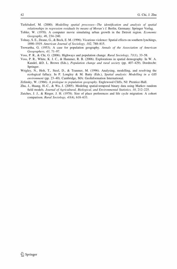
Tiefelsdorf, M. (2000). Modelling spatial processes—The identification and analysis of spatialrelationships in regression residuals by means of Moran’s I. Berlin, Germany: Springer Verlag.

Tobler, W. (1970). A computer movie simulating urban growth in the Detroit region. EconomicGeography, 46, 234–240.

Tolnay, S. E., Deane, G., & Beck, E. M. (1996). Vicarious violence: Spatial effects on southern lynchings,

1890–1919. American Journal of Sociology, 102, 788–815.

Trewartha, G. (1953). A case for population geography. Annals of the Association of AmericanGeographers, 43, 71–97.

Voss, P. R., & Chi, G. (2006). Highways and population change. Rural Sociology, 71(1), 33–58.

Voss, P. R., White, K. J. C., & Hammer, R. B. (2006). Explorations in spatial demography. In W. A.

Kandel, &D. L. Brown (Eds.), Population change and rural society (pp. 407–429). Dordrecht:

Springer.

Wrigley, N., Holt, T., Steel, D., & Tranmer, M. (1996). Analysing, modelling, and resolving the

ecological fallacy. In P. Longley & M. Batty (Eds.), Spatial analysis: Modelling in a GISenvironment (pp. 23–40). Cambridge, MA: GeoInformation International.

Zelinsky, W. (1966). A prologue to population geography. Englewood Cliffs, NJ: Prentice-Hall.

Zhu, J., Huang, H.-C., & Wu, J. (2005). Modeling spatial-temporal binary data using Markov random

field models. Journal of Agricultural, Biological, and Environmental Statistics, 10, 212–225.

Zuiches, J. J., & Rieger, J. H. (1978). Size of place preferences and life cycle migration: A cohort

comparison. Rural Sociology, 43(4), 618–633.

42 G. Chi, J. Zhu

123

Documents

Guangqing Chi Æ Jun Zhu - landdevelopability.orglanddevelopability.org/ChiWebPublications/Chi and Zhu 2008_PRPR... · or quantifying spatial patterns in the form of, ... We note