Quantifying Systemic Riskstock market crashes, the same learning principles also apply. We have shown We have shown that to quantify risk we must include the learning behavior, quantifying

This PDF is a selection from a published volume from the National Bureau of Economic Research

Volume Title: Quantifying Systemic Risk

Volume Author/Editor: Joseph G. Haubrich and Andrew W. Lo, editors

Volume Publisher: University of Chicago Press

Volume ISBN: 0-226-31928-8; ISBN-13: 978-0-226-31928-5

Volume URL: http://www.nber.org/books/haub10-1

Conference Date: November 6, 2009

Publication Date: January 2013

Chapter Title: The Quantification of Systemic Risk and Stability: New Methods and Measures

Chapter Author(s): Romney B. Duffey

Chapter URL: http://www.nber.org/chapters/c12060

Chapter pages in book: (p. 223 - 262)

223

6The Quantifi cation of Systemic Risk and StabilityNew Methods and Measures

Romney B. Duffey

6.1 The Risk Measures and Assumptions

Financial markets do not just involve money and statistics; just like all other modern systems, they include people. Therefore, to understand and predict markets it is essential to understand people, predicting their actions, mistakes, skills, decisions, responses, learning, and motivation. To under-stand people we must explicitly include their learned and unlearned behav-iors with experience and risk exposure. This is what we attempt here, based on what has been learnt from other systems data. We treat all outcomes—such as failures, crises, busts, and collapses—as occurring with some prob-ability, and that these adverse or unwelcome events refl ect the inherent stabil-ity characteristics of fi nancial markets. As noted by a well- known investor (Soros 2009): “Since markets are unstable, there are systemic risks in addi-tion to risks affecting individual market participants. . . . Participants may ignore these systemic risks . . . but regulators cannot.”

We wish to make a failure prediction, using objective measures for risk and risk exposure, since all homo- technological systems have failures and we learn from them.1 The past outcomes for all homo- technological sys-

Romney B. Duffey was the Principal Scientist at Atomic Energy of Canada Limited and is presently the principal and founder of DSM Associates Inc.

The author thanks the discussers and reviewers from the economic and fi nancial community for their insightful reactions, encouragement, criticism, comments, and suggestions on the chap-ter; the NBER for providing both the opportunity and the forum to present this work; Joseph Haubrich for proposing and pursuing the entire publication process; and AECL for supporting this research. For acknowledgments, sources of research support, and disclosure of the author’s material fi nancial relationships, if any, please see http: // www.nber.org / chapters / c12060.ack.

1. We defi ne a homo- technological system as the complex and inseparable involvement of humans in any and all aspects of design, construction, operation, management, maintenance, regulation, production, control, conduct, and decisions.

224 Romney B. Duffey

tems (industrial, transportation, production facilities) show clear evidence of trends, and the failures, busts, and crises are due to both known and unknown causes and may be “rare” or “unlikely.”

Inability to predict failures is due to the improper and incomplete treat-ment of human error, learning, and risk taking as part of the overall system. Traditional risk analysis and prediction techniques do not explicitly include the dynamic variability due to the inherent human characteristics embedded in and inseparable from the system. All major events and disasters, especially fi nancial ones, include the dominant contribution not only from individual mistakes, but also management failures and corporate- wide and regulatory errors and blunders. Risk is a measure of our uncertainty, and that uncertainty is determined by the probability of error. We must also estimate and predict risk that also includes the unknown or rare event.

We try to fi nd a dynamic objective measure that would actually anticipate instability, thus allowing predicting the onset of failure or large excursions (i.e., hence managing that risk and its consequences—equivalent to “emer-gency preparedness”). In the popular fi nance articles, the risk mitigation pro-cess seems to be referred to as “pricking bubbles,” and traditionally involves some kind of ad- hoc debt, credit and trading limitations, and / or restraints. These types of regulation or reactions are very much a posteriori and case- by- case, but are neither predictive nor general. As noted for risk in Nature Nanotechnology: “the real issue is how to regulate in the face of uncertainty” (Brown 2009, 209). Our work suggests that learning is effective as a risk management and predictive tool, but only if we have adopted the “correct” risk exposure and uncertainty measures that we now attempt to determine.

Obviously, as humans we learn from experience, both good and bad. We also take risks and must make mistakes in order to improve. A universal curve is derived for both collective and individual learning trends, naturally including the inevitability of outcomes and risk. Based on our work study-ing and analyzing over 200 years of real data on and for risk in technologi-cal, medical, industrial, and fi nancial systems, fi ve measures are presented and discussed for the objective measure of risk, failure probability, and risk exposure. Correct measure(s) for experience enable the prediction and uncer-tainty estimation for the entire range of rare, repeat, and unknown outcomes (e.g., major industrial disasters, facility accidents and explosions, everyday auto accidents, aircraft crashes, fi nancial busts, and market collapses).

We also introduce and present the unifying concept of risk and uncer-tainty derived from the information entropy as a quantitative measure of randomness and disorder. We show how this allows comparative risk esti-mation and the discerning of insufficient learning. Since these risk mea-sures and learning trends have been largely derived from data including the fi nancial arena, we show how to generalize these to include the presence of market pressures, fi nancial issues, and risk measures. We defi ne and present the bases, analyses, and results for new risk measures for the quantitative

The Quantifi cation of Systemic Risk and Stability 225

predictions of risk exposure, failure, and collapse using relevant experience including:

1. Universal Learning (ULC), similar to the Black- Scholes concept2. Risk Ratios (RR) and exposure, as derived from empirical hazard

curves3. Repeat Event Predictions (REP) or never happening again, equivalent

to birthday matching and reoccurring echoes4. Rare and Unknown Outcome occurrences (UU), as in the black swan

concept5. System and Organizational Stability (SOS) or resilience criteria, using

the information entropy concept

We provide quantifi ed examples for production processes, transportation losses, major hazards, and fi nancial exposure. These new concepts also pro-vide the probability of success, the emergence of order, and the understand-ing and quantifi cation of risk perception. Note that these measures replace and do not include in any way the standard fi nancial techniques utilizing net value, value at risk, or variations about or from the mean.

In our analysis we assume fi nancial markets are just another homo- technological system and the past failure rates inform the future, and that the inherent apparent randomness and chaos conveys and contains infor-mation. We avoid using traditional statistical approaches where past failure frequencies defi ne invariant future failure probability distributions. We also explicitly avoid the impossible modeling of all the internal details of assets and trading, and avoid any fi ltering of data; we consider only emergent trends at system level based on what we know. We treat risk as determined by experience or risk exposure, thus avoiding using comfortable calendar time intervals (i.e., as in daily, hourly, monthly, quarterly, or annual report-ing) as markets operate according to their experience. As in medical and other systems, this risk measure is often determined by the dynamic accumu-lated “volume,” which also provides the learning opportunity. Our research approach is predicated on extrapolating known and unknown past failure rates based on experience and future dynamic risk exposure, and is tested against data, so the concept and measures of risk and stability are truly falsifi able.

6.2 Risk: How We Learn from Experience and What We Know about Risk Prediction

Risk is measured by our uncertainty, and the measure of uncertainty is probability.

The defi nition, use, and concepts of risk adopted in this chapter utilizes measures for risk exposure and for uncertainty that encompass and are con-sistent with that proposed before in the fi nancial literature (Holton 2004, 19):


Risk entails two essential components:

• Exposure, and• Uncertainty

Risk, then, is exposure to a proposition of which one is uncertain.

What is the risk of system failure? What is the measure for exposure? What is the measure of uncertainty? To answer those questions we must understand how and why systems fail, and show how to make a prediction, noting that while fi nancial systems constitute a distinct discipline with its own terminology, they actually must behave just like all others that are prone to the all too common vagaries, actions, and motivations of humans. We use probability and information entropy to quantify uncertainty, and past and future experience to quantify exposure.

We fi rst review what is known and not known about predicting and man-aging risk in industrial, energy, transportation, nuclear, medical, and manu-facturing systems, and the associated risk exposure measures. We address the question of the predictability of a large systems failure, or collapse, and the necessary concepts related to risk quantifi cation and system stability that are emerging from the physical sciences, cognitive psychology, information theory, and multiple industrial arenas that are relevant to current fi nancial and economic market and stability concerns. We have defi ned the risk of any outcome (being a proposition of which one is uncertain) as caused by uncertainty, and that the measure of the uncertainty is probability, p. We attempt to use some of these risk concepts, learning, and applications from mainly operational systems to inform risk prediction for fi nancial systems.

Risks are due to the probability / possibility of an adverse event, out-come, or accident. Simply put, we learn from our mistakes, correcting our errors along the way. We all know that we have had a serious failure of the fi nancial and investments markets due to excessive risk exposure and losses. The key observation is that markets are random, which is confi rmed by sampling distributions, but we also know that conventional statistics of normal distributions (such as used in VaR and CoVaR techniques) do not work when applied to predicting dynamically changing accident, event, and outcome trends (Taleb 2007; Duffey and Saull 2008). So while the instanta-neous behavior appears to be random and hence unpredictable, the failure to predict is due to the failure to properly include the systematic infl uence of human element, which is nonlinear, dynamic, and varies with experience and risk exposure.

In industrial operations, the cardinal rule of operation applicable to any system is due to Howlett (2001), which is:

Humans must remain in control of their machinery at all times. Any time the machine operates without the knowledge, understanding and assent of its human controllers, the machine is out of control. (5)


Furthermore, the limits to operation are defi ned by a Safe Operating Enve-lope, with limits that include margins and uncertainty that defi ne “guaran-tees” for the avoidance of failure. Risk management is then employed to protect or mitigate the consequences of failures that might occur anyway (Howlett 2001). These well- tried concepts are all translatable to and usable in fi nancial systems, just as they are for industrial systems, since all systems include human involvement and hence involve the uncertainty due to risk tak-ing and learning.

We have previously shown that the dominant contribution to all manage-ment and system failures, outcomes, and accidents is from that same inextri-cable and inseparable human involvement. Be they airplane, auto, train, or stock market crashes, the same learning principles also apply. We have shown that to quantify risk we must include the learning behavior, quantifying out-comes rates, and probabilities due to our experience from human decision making and involvement with modern technological and social systems, including industrial, transportation, chemical, fi nancial, and manufactur-ing technologies (Duffey and Saull 2002, 2008). These ideas and concepts include naturally not only the collective system (e.g., a bank, railway, power plant, or airline) but also the individual human reliability (e.g., an investor, driver, manager, or pilot).

What we know is that provided we have prior (outcome or failure) data we can now predict accurately the future outcome rates, and defi ne the risk exposure based on the past known and the future expected experience. That we can learn from experience is what all the data show, and that experience is the past risk exposure we have all so painfully acquired as a human society. The experience measure is a surrogate for our very human risk exposure, of how long, how many, and how much we have been exposed to the chance of an outcome, or to the risk of an error.

The prediction of the future rate of failures or outcomes is given from the Learning Hypothesis, being simply the principle that humans naturally learn from their mistakes, by correcting and unlearning during and from the accumulated experience, both good and bad. The experience—however it is defi ned or measured—represents also not only the learning opportunity, but a measure of the risk exposure. The probability of error, accident, catas-trophe, or mistake ( p) is determined by the failure rate, which derives from the number of either a successful or a failed (unsuccessful) outcome. The rate of outcomes decreases exponentially with experience, in the form of a Universal Learning Curve (ULC). Over 200 years of experience and millions of prior, past, or historic data allow the ULC to be defi ned. The validation derives from massive data sets of both frequent and rare events (Duffey and Saull 2002, 2008), which now includes multiple sources and outcomes, with the historical time spans covering the past 200 years, and major data avail-able from the last 50 or more years.


We analyzed auto passenger deaths, railway injuries, coal mining deaths, oil spills at sea, commercial airline near- misses, and recreational boating deaths. Globally, the learning data set we have amassed now contains mul-tiple technologies worldwide: coal and gold mining, 20 million pulmonary disease deaths, cataract operations, infant heart surgeries, the international total of rocket launches, pilot deaths in Australia, train derailments and danger signals passed on railways, and notably, the anti- missile interception and destruction effectiveness over England of German VI bombs in World War II. Economic data on specifi c unit price variations with increasing out-put or commercial sales demonstrating the learning trends and so- called “progress curves” for manufacturing are observed for millions of units pro-duced in factories and production lines.

The millions of outcome data analyzed are well represented by the Learn-ing Hypothesis (Duffey and Saull 2002, 2008), which states that the rate of decrease of the outcome or failure rate, �, with experience units, �, is proportional to that same rate. Thus, very simply, the differential equation is the proportionality:

d�

d�

⎛⎝⎜

⎞⎠⎟

∝ �.

The previous cases and data sets show variations in the learning constant: when learning trends are present an average learning rate “constant” of proportionality value of k ~ 3 is reasonable (see also fi gure 6.1).

Systems exist that do not show signifi cant learning, as measured by decrease or declining loss and error trends, are those where the continuing infl uence and reliance on the human element and historic practices overrides massive changes in technology and the robustness of system design.

6.3 Individual Actions: Predictable and Unpredictable

It is reasonable to ask how the behavior of entire systems refl ect the indi-vidual interactions within them, and vice versa, including the myriads of managers, accountants, traders, investors, speculators, lawyers, and regula-tors that make up a fi nancial market or system. This link is between the unobserved multitudinous and microscopic interactions and the observed macroscopic and emergent system trends, distributions, responses, and out-comes. For just individual actions (as opposed to system outcomes), data are available in the psychological literature from many thousands of individual human subject task and learning trials. These trials have established the rate of skill acquisition as described by the so- called Laws of Practice. We have shown (Duffey and Saull 2008) that these laws are entirely consistent with the ULC for entire systems and have the same learning constant (or K value) with repeated trials. Thus, the data show that external system- learning behavior mirrors the internal learning trends of the individuals within. The


predicted probability of error also agrees with published nuclear plants events, simulator tests, and system recovery action times. Probabilities for power restoration for power losses at over 100 US nuclear power plants are also in agreement, as is the power blackout repair probability for customers over a period of several days.

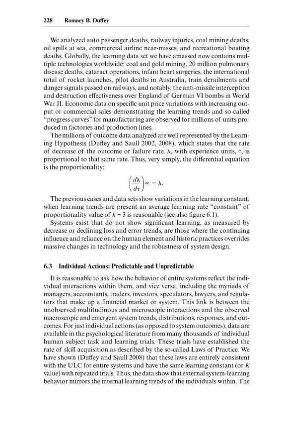
In all these data, we have n outcomes occurring in some experience, �. The resulting form of the learning curve is shown in fi gure 6.1, which is a log- log plot with arbitrary units on each axis of the rate of the undesirable errors and outcomes, dn / d�, versus the accumulated experience, which is a surro-gate for the risk exposure during actual system operation. This risk exposure or experience measure, �, is unique for each and every system: for aircraft it is the number of fl ights fl own, for railways the train- miles traveled, for ships the shipping- years afl oat, for manufacturing the number of units produced, for human errors in decision making, skill acquisition, and response time it is the number of repetitive trials.

As we increase our experience and risk exposure as both individuals and systems, the event or outcome rate depends on whether, either collectively and / or individually, we follow a learning curve of decreasing risk or not, or if we are somewhere in between. In fi gure 6.1, the line labeled “learning curve” (from the Minimum Error Rate Equation, or MERE) is the desirable ULC, where learning occurs to rapidly reduce the rate. This is the most likely path, and is also that of the least risk as we progress from being a “novice” with little experience to becoming an “expert with progressively more exposure

Fig. 6.1 The ULC and Constant Risk Lines: Failure rates with increasing experi-ence and / or risk exposure


and experience.” There are no “zero defects”; there is always a fi nite, nonzero residual rate of error, �m, so say all of the world’s data. The equation that describes the learning curve is an exponential with experience:2

Failure rate, �(�) � Minimum rate, �m

� (Initial rate, �0 Minimum rate, �m) � exp(k�).

If we simply replace the rate, �, by the value or specifi c cost, C, and change the sign, the MERE turns out to be identical in form to that of the trend-ing part of the Black- Scholes equation for portfolio cost and value. For manufacturing or production there is a “tail” of nonzero value that cor-responds to the minimum possibly achievable, Cm, in any competitive mar-ket system. Reducing cost with increasing volume, or units produced, thus also holds for manufacturing and production cost decreases, just as patient volume does for improving individual surgical skill, thus reducing inadver-tent deaths with increasing patient count (practice or trials). The difference is that in these cases the experience parameter, �, is conventionally taken as either time (for stock or equity values variation) or accumulated units manufactured (for production prices changes), and a key question is what measure to adopt in fi nancial systems for the relevant experience and risk exposure.

Since fi gure 6.1 is a log- log plot (scale units are factors of ten on each axis), any line of constant risk is then a straight line of slope minus one, where the event rate, �, times experience, �, is the constant number of events, n. Hence, � � n / �, and for the fi rst or rare event, n � 1, which is the dashed “constant risk” line for any fi rst or rare event shown in fi gure 6.1. The rate decreases inversely with the risk exposure or experience, so importantly, at little or no experience or little learning, the initial rate is given by �0 � 1 / �, which is exactly the form of the rare events as derived from commercial aircraft crashes. As we shall see, this risk path is the initial rate and also emphasizes the “fat tail” that worries and confounds conventional risk and value ana-lysts. We call this prediction a White Elephant when it underestimates the risk, since it has no value as a prediction.

In terms of probabilities as a measure of risk, instead of rates, the pre-vious equation can be integrated to yield an expression that in words implies:

Risk exposure probability is due to the minimum risk plus the initial risk exposure less the reduction in risk due to learning.

For any real, not hypothetical system the minimum achievable failure rate does not appear to change and has not changed for over 200 years, depend-ing solely on our experience and risk exposure measure for a given system. So conversely, the systemic risk (the probability of failure or a bust) is dependent on the risk exposure measure.

2. See the defi nitions and derivations in the appendix.


6.4 The Seven Commonalities of Rare and Terrible Events: Risk Ratios and Predictions

What do large disasters, crises, busts, and collapses in fi nancial systems like the Great Crash of 2008 (IMF 2009b) have in common with the other major events? These have happened in multiple technologies and indus-tries, such as in industries as diverse as aerospace (Columbia and Challenger Shuttle losses) (CAIB 2003), nuclear (Davis- Besse plant vessel corrosion) (NRC 2008), oil (Deepwater Horizon explosion and leak) (US National Commission 2011), chemical (Toulouse ammonia plant explosion) (Bar-thelemy 2001), transportation (the Quebec overpass collapse) (Commission of Inquiry 2007a, 2007b), and the recent devastating nuclear reactor melt-downs at the Fukushima plants in Japan. The common features, or, as we may call them, the Seven Themes, cover the aspects of causation, rationaliza-tion, retribution, and prevention, ad nauseam.

First, these major losses, failures, and outcomes all share the same very same and very human Four Phases or warning signs: the unfolding of the precursors and initiating circumstances, the confl uence of events and circum-stances in unexpected ways, the escalation where the unrecognized unknow-ingly happens, and afterward, denial and blame shift before fi nal acceptance.

Second, as always, these incidents all involved humans, were not expected but clearly understandable as due to management emphasis on production and profi t rather than safety and risk, were from gaps in the operating and management requirements, and from lax inspection and inadequate regula-tions.

Third, these events have all caused a spate of media coverage, retroactive soul- searching, “culture” studies and surveys, regulation review, revisions to laws, guidelines, and procedures, new limits, and reporting legislation, which all echo perfectly the present emphasis on limits to the bonus culture and risk taking that are or were endemic in certain fi nancial circles.

Fourth, the failures were so- called “rare events” and involved obvious dynamic human lapses and errors, and as such do not follow the usual sta-tistical rules and laws that govern large quasi- static samples, or the multi-tudinous outcome distributions (like normal, lognormal, and Weibull) that dominate conventional statistical thinking, but clearly require analysis and understanding of the role of human learning, experience, and skill in making mistakes and taking decisions.

Fifth, these events all involve humans operating inside and / or with a sys-tem, and contain real information about what we know about what we do not know—being the unexpected, the unknown, the rare and low occurrence rate events—with large consequences and highlighting our own inadequate predictive capability, so that to predict we must use Bayesian- type likelihood estimation.

Sixth, there is the learning paradox that if we do not learn we have more


risk, but to learn perversely we must have the very events we seek to avoid, which also have a large and fi nite risk of reoccurrence. Ultimately, we have more risk from events we have not had the chance to learn about, being the unknown, rare, or unexpected.

Seventh, these events were all preventable but only afterward. Hindsight, soul- searching, and sometimes massive inquiries reveal what was so obvious time after time—the same human fallibilities, performance lapses, super-visory and inspections gaps, bad habits, inadequate rules and legislation, management failures, and risk- taking behaviors that all should have been and were self- evident, and were uncorrected.

We claim to learn from these each time, perhaps introducing corrective actions, revised rules, and lessons learned (Ohlsson 1996), thus hopefully reducing the outcome rate or the chance of reoccurrence. All of these aspects were also evident in the fi nancial failure of 2008, in the collapse of major fi nancial institutions and banks. These rare events are worth examining fur-ther as to their repeat frequency and market failure probability: recessions have happened before but 2008 was supposedly somewhat different, as it was reportedly due to unbridled systemic risk, and uncontrolled systemic failure in credit and real estate sectors. This failure of risk management in fi nan-cial markets led to the analysis that follows, extending the observations, new thinking, and methods developed for understanding other technological sys-tems to the prediction and management of so- called “systemic risk” in fi nan-cial markets and transactions. We treat and analyze these fi nancial entities as systems that function and behave by learning from experience just like any other system, where we observe the external outcomes and failures due to the unobserved internal activities, management decisions, errors, and risks taken.

The past outcome data provide the past failure rate. To determine the future risk, we must distinguish between the past (statistically, the known prior) and the future (statistically, the unknown posterior). So what does the past tell us about the future? To predict an outcome, any event, we must go beyond what we know, that is, the prior knowledge. Somehow, we have to project ourselves into an unknown future, with some measure of confi dence and uncertainty, based on both our rational thoughts and our irrational fears, using what we know about what we do not know. This leads us into the somewhat controversial arena of prediction using statistical reasoning, a subject addressed in great detail elsewhere (Jaynes 2003).

The conditional future is dependent, albeit with uncertainty, on the past, as per Bayes reasoning (Jaynes 2003; Bayes 1763, 376). The probability or chance of an unknown event is dependent on something called the likeli-hood, which itself is uncertain but provides a rational framework for pro-jection. The likelihood itself is inversely dependent on the prior number of outcomes, and if there are none so far, we just have the Bayesian failure rate of the past based on our (known) experience to date.

The Likelihood formally adjusts the past, prior, or known probability and


produces the future or posterior probability. So conditionally dependent on what we already know we know has already happened in the past, according to the thinking of the Reverend Thomas Bayes (1763) and of Edwin Jaynes’ (2003) rigorous analysis:

Future chance (posterior probability, p(P))

� Past or prior probability, p, times Likelihood.

The Likelihood multiplier, p(L), whatever it is and however derived (by physical argument, guess, judgment, evidence, probabilistic reasoning, mathematical rigor, or data analysis) is the conditioning factor that always alters the past whatever and however it is estimated. Even if the past was indeed “normal,” the likelihood can even change the future to include rare events and unknown unknowns.

The risk ratio (RR) can then be defi ned as ratio of the future posterior probability, p(P), of an adverse event (accident, outcome, error, or failure in the future) to some known past or present failure probability, p(�), based on the prior accumulated experience, as a function of the future risk exposure or experience, or

RR �

p(P)p(�)

.

From the above Bayesian equation this risk ratio is equivalent to defi ning the Likelihood, p(L), where for low probabilities or rare events the posterior, p(P), itself is numerically very nearly equal to the rate of events, or the failure rate, p(P) ~ f(�) ~ �. This result follows directly from the so- called “general-ized Bayes formula” (Sveshnikov 1968 49, 80; Duffey and Saull 2008) that defi nes the Likelihood as the ratio of the probability of outcomes occurring in the next experience interval to the probability that outcomes have already occurred during the past experience.

So for low probability events, outcomes, or disasters ( p(�) �� 1), the risk ratio becomes simply the future predicted by the past since:

RR �

p(P)(1 − p(�))p(�)

~

p(P)p(�)

~

�(�)p(�)

,

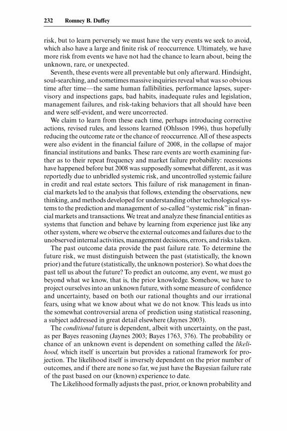
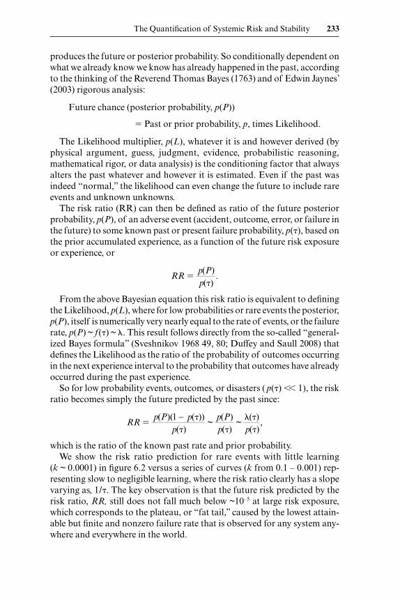
which is the ratio of the known past rate and prior probability.We show the risk ratio prediction for rare events with little learning

(k ~ 0.0001) in fi gure 6.2 versus a series of curves (k from 0.1 – 0.001) rep-resenting slow to negligible learning, where the risk ratio clearly has a slope varying as, 1 / �. The key observation is that the future risk predicted by the risk ratio, RR, still does not fall much below ~10–5 at large risk exposure, which corresponds to the plateau, or “fat tail,” caused by the lowest attain-able but fi nite and nonzero failure rate that is observed for any system any-where and everywhere in the world.


So what, then, is the resulting Posterior probability, p(P) in the future? It is shown in fi gure 6.2 for a series of cases with varying learning or knowl-edge acquisition from increasing risk exposure or accumulated experience. These cases are represented by the range of values shown for the learning “constant,” k, where progressively lower values mean less and less learning. As can be seen, if learning is negligible so that k is very small (say, 0.0001) then the event probability decreases almost as a straight line of constant risk, 1 / �, as it should; for larger k values a distinct kink or plateau occurs due to the presence of the always fi nite, nonzero failure rate due to the human involvement.

6.5 Predicting Rare Events: Fat Tails, Black Swans, and White Elephants

Colloquially, a Black Swan is an unexpected and / or rare event, one that dramatically changes prior thinking and expectations.

Because rare events do not happen often, they are also widely misun-derstood. Perhaps even previously unobserved, they are called “unknown unknowns” (Rumsfeld 2002), or “Black Swans” (Taleb 2007) precisely because they do not follow the same rules when already having many or frequent events. Think of the space shuttle crashes, the global collapse of fi nancial companies, or an aircraft apparently falling from the sky as it did recently over the Atlantic. These are the things we may or may not have seen before, but certainly did not expect to happen. So when they do happen, perhaps even when being thought not possible, they do not apparently fol-

Fig. 6.2 Comparisons of the Risk Ratio Predictions


low the trends, expectations, rules, or knowledge we have built up for more frequent happenings.

There is no assured, easy, or obvious “alarm,” indicator, or built- in warn-ing signal, derivable by adjusting fi lters or data smoothing techniques. As noted in World Bank (2009),

Whether these alarms are deemed informative depends on their associa-tion with subsequent busts. The choice of a threshold above which an alarm is raised presents an important trade- off between the desire for some warning of an impending bust and the costs associated with a false alarm. Nonetheless, even the best indicator failed to raise an alarm one to three years ahead of roughly one- half of all busts since 1985. Thus, asset price busts are difficult to predict.

This is a 50 percent or even chance, which are no better odds than just toss-ing a coin.

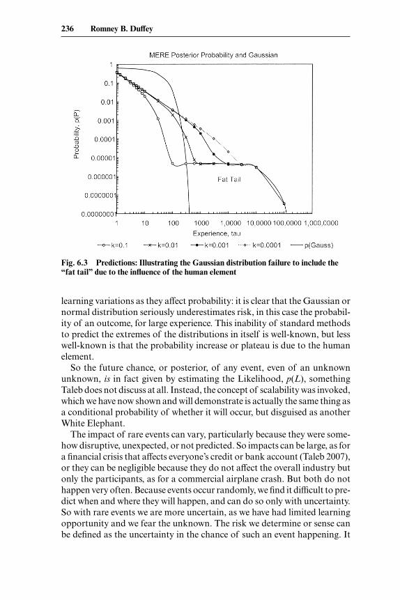
In statistical language and usage, the rare events do not follow or fi t in with the usual distributions of previous or expected occurrences. The frequency and / or probability of occurrence lies somewhere outside the usual many expected multiples of the standard deviation for any sample distribution. We may not even have a distribution of prior data anyway. In fact, Taleb (2007) spends a considerable part of his popular book The Black Swan discuss-ing, discounting, and dismissing the use of so- called normal distributions such as the Gaussian or bell- shaped curves simply because they do not and cannot account for rare events even though many humans may think that they do. Also rare events, like all events, as we have said, are always due to some apparently unforeseen combination of circumstance, conditions, and combination of things that we did not foresee, and all include the errors in our human made and managed systems (the Seven Themes).

By citing many empirical cases, Taleb (2007) also further argues forcibly that this scale variation destroys any and all credibility of using any Gauss-ian or normal distribution for prediction. In that limited sense, he is right, as conventional sampling statistics based on fi tting to some normal distri-butions using many observations is totally inapplicable for low probability, one- of- a- kind rare, so- far- unobserved or unknown events. To make a true prediction we must still use what we know about what we do not know, and we now know that the relevant “scale” is in fact our experience or risk expo-sure, which is what we have anyway, and is the basis for what we know or do not know about everything.

In fi gure 6.3, we show the one- on- one head- to- head comparison of a normal (Gaussian) bell- shaped distribution,3 compared to the reality of

3. The example Gaussian (or normal) distribution shown in fi gure 6.3 is p(P) � 23 exp(–0.5 (� � 290) / 109)2, and was fi tted to the MERE learning curve using the commercial statistical software routine TableCurve 2D.


learning variations as they affect probability: it is clear that the Gaussian or normal distribution seriously underestimates risk, in this case the probabil-ity of an outcome, for large experience. This inability of standard methods to predict the extremes of the distributions in itself is well- known, but less well- known is that the probability increase or plateau is due to the human element.

So the future chance, or posterior, of any event, even of an unknown unknown, is in fact given by estimating the Likelihood, p(L), something Taleb does not discuss at all. Instead, the concept of scalability was invoked, which we have now shown and will demonstrate is actually the same thing as a conditional probability of whether it will occur, but disguised as another White Elephant.

The impact of rare events can vary, particularly because they were some-how disruptive, unexpected, or not predicted. So impacts can be large, as for a fi nancial crisis that affects everyone’s credit or bank account (Taleb 2007), or they can be negligible because they do not affect the overall industry but only the participants, as for a commercial airplane crash. But both do not happen very often. Because events occur randomly, we fi nd it difficult to pre-dict when and where they will happen, and can do so only with uncertainty. So with rare events we are more uncertain, as we have had limited learning opportunity and we fear the unknown. The risk we determine or sense can be defi ned as the uncertainty in the chance of such an event happening. It

Fig. 6.3 Predictions: Illustrating the Gaussian distribution failure to include the “fat tail” due to the infl uence of the human element


is perceived by us, individually and collectively, as being a high risk or not based on how we feel about it, and have been taught, trained, experienced, learned, or indoctrinated. The randomness is then inherent in the learning processes, in the myriad of learned and unlearned patterns, neural fi rings, legal rules, acquired skills, written procedures, unconscious decisions, and conscious interactions that any and all humans have in any and all systems. Perversely, only by having such randomness, learning, skill, trial, and error can order and learning patterns emerge. We create order from disorder, learning as we go from experience and risk exposure, discerning the right and unlearning the wrong behaviors and skills. So a rare Black Swan, even if of major impact, is indeed a White Elephant of no intrinsic value unless and only if we are learning.

We need to know what we do not know. We cannot know what happens inside our brains and see the how the trillions of neural patterns, path-ways, and possibilities are wired, learned, interconnected, rationalized, and unlearned. We cannot know the millions of things that any group of people will talk about, learn, exchange, review, revise, argue, debate, reject, use and abuse, each and every day. We cannot know all about how a machine or system will behave when subjected to the whims of inadequate design, poor maintenance, extreme failure modes, external damage, and poor or unsafe operation. What we do know is that, because we are human, we do learn from our mistakes: this is the Learning Hypothesis (Petroski 1985; Ohlsson 1996; Duffey and Saull 2002). The rate at which we make errors, produce outcomes, and cause events reduces both as we gain experience and if and as we learn. We make mistakes because we are human: the fat tail, the rare event, occurs because we are human. If and as we gain experience, this is equivalent to increasing our risk exposure too. The risk increases whether by driving on the road, by trading stocks and investments, or by building and operating a technological system like a ship, train, rocket, or aircraft.

Consistent with the principles of natural selection, those who do not learn, those who do not adapt and survive, are the failures and extinctions of history, overtaken by the unexpected and mistakes, the errors and the Black Swans of the past.

6.6 Failure to Predict Failure: Scaling Laws and the Risk Plateau

What do we know about what we do not know? We know that the four categories of knowns and unknowns are the Rumsfeld quartet:

Known knowns: What is expected and already observed (in the past)Known unknowns: Unexpected but observed outcomes (past outcomes)Unknown knowns: Expected and not yet observed (in the future)Unknown unknowns: Unexpected and not yet observed (future outcomes

or rare events)


This is analogous to drawing both outcomes and nonoutcomes from Ber-noulli’s urn (Duffey and Saull 2008), and the probability of a rare (unknown) event is determined if all we do is assume that it exists. Thus, we have turned a Black Swan into a White Elephant—the fact that we have not observed it, do not know if it exists, but can rationally discuss it allows the fear, dread, and risk perception to be quantifi ed. This is precisely what Taleb recom-mends—taking precautions against what it is we do not know about what we do now know.

We have defi ned a risk ratio that depends on the prior failure rate. But for a rare or unknown event the posterior probability of an unknown unknown, p(U, U ) that has not happened yet is fi nite and is given by analogy to the “case of zero failures” in purely statistical analysis (Coolen 2006, 105). We can then obtain the mathematical estimate for knowing the posterior (future) probability of the unknowable as Duffey and Saull (2008):

P(U, U ) ~

1U�2

⎛⎝⎜

⎞⎠⎟ exp- U,

where U is some constant of proportionality. This order of magnitude esti-mate shows a clear trend of the probability decreasing with increasing expe-rience as an inverse square power law, �2. For every factor of ten increase in experience measured in some tau units, �, the posterior probability falls by one hundred times. It does not matter if we do not know the exact numbers: the trend is the key for decision making and risk taking. The rational choice and implication is to trust experience and not to be afraid of the perceived Unknown.

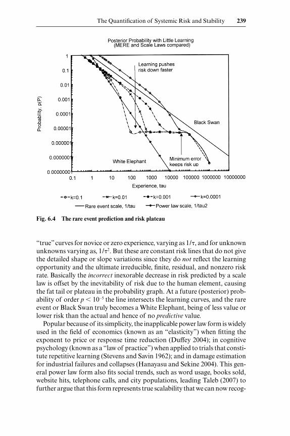
But although useful for comparative trending purposes, such a purely statistical analysis excludes the key human involvement and uncertainty con-tribution. Hence the risk of an unknown unknown decreases inexorably with our increasing experience, or risk exposure, only until a risk plateau is reached and no further decrease in probability is possible. Therefore, con-tinuing to extrapolate using such scaling power laws will always ultimately underestimate risk. So the White Elephant is precisely the case of little or no learning corresponding exactly to a scaled probability inverse law, that is, p(P) � n / �, where the number of events, n, is one (n � 1), simply because it is that fi rst and rare event that was never previously observed or known. So the probability, p, of any single rare event is always, 1 / �, the inverse of (one divided by) the exposure or experience measure, or scale. As shown before in fi gure 6.2, this is also a measure of the risk ratio and is equivalent numerically to the failure rate, �. So also shown in fi gure 6.4 are the so- called “scalable” or pure “power” laws discussed by Taleb (2007), where the prob-ability is assumed to fall as the more general inverse power law, p(P) � l / � .

Corresponding to the prior and the posterior variations without signifi -cant learning, for illustration, the “slope” parameter, , is often taken as lying in the range between 1 and 2, which assumed values nicely cover the


“true” curves for novice or zero experience, varying as 1 / �, and for unknown unknowns varying as, 1 / �2. But these are constant risk lines that do not give the detailed shape or slope variations since they do not refl ect the learning opportunity and the ultimate irreducible, fi nite, residual, and nonzero risk rate. Basically the incorrect inexorable decrease in risk predicted by a scale law is offset by the inevitability of risk due to the human element, causing the fat tail or plateau in the probability graph. At a future (posterior) prob-ability of order p � 10–5 the line intersects the learning curves, and the rare event or Black Swan truly becomes a White Elephant, being of less value or lower risk than the actual and hence of no predictive value.

Popular because of its simplicity, the inapplicable power law form is widely used in the fi eld of economics (known as an “elasticity”) when fi tting the exponent to price or response time reduction (Duffey 2004); in cognitive psychology (known as a “law of practice”) when applied to trials that consti-tute repetitive learning (Stevens and Savin 1962); and in damage estimation for industrial failures and collapses (Hanayasu and Sekine 2004). This gen-eral power law form also fi ts social trends, such as word usage, books sold, website hits, telephone calls, and city populations, leading Taleb (2007) to further argue that this form represents true scalability that we can now recog-

Fig. 6.4 The rare event prediction and risk plateau


nize as the fundamental connection to learning and risk exposure. Arbitrary adjustment of the exponent, , in economics, social science, and cognitive psychology is an attempt to actually account for and fi t what we observe, but without trying to understand why the exponent is not unity nor placing limits on the extrapolations made beyond the known data used for the original fi ts.

The exponent is roughly constant only over limited ranges of data, other-wise it fails in extrapolating magnitude or trend (Duffey and Saull 2008). In fact in statistics, this form of inverse power law type of relation is often known as a Pareto distribution4 and Woo (1999, 224) explicitly further cau-tions that “parameterizing a natural hazard loss curve cannot be reliably reduced to a statistical analysis of loss data, e.g., fi tting a Pareto curve: damaging events are too infrequent for this to be sound.”

In fact, this failure to predict may even explain the proven poor capabil-ity of many economic models, which by using a constant elasticity between price and demand and extrapolating we now know from data do not predict well! We now know and can see from fi gure 6.4 that the exponent is not con-stant and the variation in reality is due to the presence and effects of learn-ing, with the larger exponent values and steeper slope encompassing the variation between the learning curves (fi gure 6.3). This variation represents uncertainty and constitutes the measure of risk if taken as a technique for making investment decisions.

Figures 6.3 and 6.4 contain much useful information. Not only are the trends with learning clear, there is the tendency for risk to be smaller initially with more learning; and greater at larger experience due to the forming of a plateau of nearly constant risk (a fat tail, or potential Black Swan). If we neglect this large human contribution and effect at large risk exposure then Pareto lines, power laws, normal and lognormal distributions become White Elephants of little value, as being extrapolated they underestimate the risk. A similar argument can be made for not using results from static or equilibrium VaR and CoVaR techniques (see Taleb [2007], the papers presented at the NBER systemic risk conference, and the chapters in this book).These tech-niques fi t standard statistical distributions to fi nancial asset data and then seek signifi cance in the differences and trends out at the 1 to 2 percent tail, while ignoring again the dynamic human contribution and hence unaware of and not accounting for the systematic existence of the systemic risk plateau.

This presence of learning effects nicely explains the actual range of empir-ical values for the exponent, , quoted by Taleb and others of between 1 and 2—some systems evidently exhibit more or less initial learning than oth-ers, as is shown in fi gure 6.4. Including the statistical limit of unknown unknowns, the inverse power law simplifi cation shows by defi nition that if

4. Also termed the hyperbolic or power law distribution, the form given by Woo for natu-ral catastrophes is p(�) � bab / �b�1, where a and b are constants, the so- called “location” and “shape” parameters.


there are no events there is and can be no learning. Strictly, we know this is not true, as we also learn something from the many and often irritating nonevents, minor losses, and near misses. This so- called incidental learning leads to the other extreme case of “perfect learning” (Duffey and Saull 2008), where the event outcome probability still follows a learning curve until we have just one event, and then subsequently plummets to zero.

We stress here that the power law form is a natural, simplifi ed limiting vari-ant of the more general “learning curve,” which naturally then also encom-passes the occurrence of rare events.

The analysis of risk ratios due to the fi nancial cost of individual events assumes that big losses or damage occur less often (i.e., are rare or lower in frequency). For example, Hanayasu and Sekine (2004) argue that the rate of fi nancial damage of events in industry decreases with the inverse of the dam-age or loss. So generally the frequency of an event decreases with increasing cost as the probability density,

dpd�

≈

constanthq +1

.

Here, q is yet another power law exponent chosen to fi t some damage data, and is always such that q � 1, so Hanayasu and Sekine assume that it lies in the range 2 � q � 3. When the slope is an inverse cube such that ~ 3, there is a very rapid decline. We analyzed this approach (Holton 2004, 19) and found the risk ratio or damage ratio referenced to some initial known value, h0, and probability, p0, is then given by:

RR �

hh0

⎛⎝⎜

⎞⎠⎟

�

pp0

⎛⎝⎜

⎞⎠⎟

1/q

.

Extrapolation of the fi tted line beyond the data range given shows a much faster decrease in risk ratio than usually observed or expected from a learn-ing curve with a fi nite minimum that fl attens out. So the basic problem is that extrapolation of the size of the loss according to this power law (although it is not really a law at all) produces inaccuracy outside the known data range, does not account for learning, and also does not allow for the fi nite nonzero contribution of the human element (the extra fat tail shown in fi gure 6.2). We have fi tted a MERE curve also to these damage data, and as a result the forward risk exposure, fi nancial loss, or uncertainty is grossly underestimated because of omitting the human learning element. This is really uncertainty: we are predicting the variation in how big the losses will be for unknown events, based on what we know.

The chance of an unknown unknown or rare event also depends on whether or not you learn! Conversely, rare events and Black Swans are also simply events for which we have little or no learning. The argument is then wrong that this type of inverse power variation represents true random-ness, where there is no pattern other than that which is scale invariant (like


fractals). In fact, the variation in probability or risk in reality is all due to whether we have been learning or not, at what rate we make or have made mistakes both in the past and in the future. The true natural scale for all human- based systemic risk we have shown repeatedly is our experience, however that is defi ned and accumulated, as learning is not invariant with risk exposure. What we know about the unknown is that we are human and remain so, learning as we go.

For the future unknown experience, the average future failure rate, ⟨�⟩, we will observe over any future risk exposure or operating interval, � – �0, that is obtained by averaging the varying failure rate over that same observation or risk exposure interval, so:

⟨�⟩ �

1(� − �0)

�

�0

∫ �(�)d�.

Clearly, the apparent average rate also depends on the risk exposure inter-val, � – �0, over which we start and fi nish observing, or choose to record outcomes, or happen to be present, or are risk exposed.

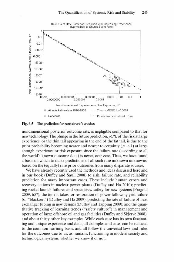
We can show how these ideas work in practice by comparing to actual data for rare events, although this is strictly an oxymoron, as if the outcomes occur they are no longer rare or become known unknowns. The data avail-able is the case we have analyzed in detail before (Duffey and Saull 2002, 2008), for fatal commercial airline crashes between 1970 and 2000. The case is relevant as the airline industry is regarded as relatively safe, and having perhaps attained the lowest possible event rate. Over this thirty- year period using modern jets, some 114 commercial passenger airlines accumulated about 220 million fl ights, and there were about 270 fatal crashes, excluding hull losses (plane write- offs), with no deaths. The data show a lack of further learning trends, as airline crashes attain the lowest rate currently known or achievable of about one per 200,000 fl ying experiences or risk exposure hours. What has actually happened is that because they have become rare events there is an almost constant risk, as shown in fi gure 6.5, where the fatal crash rate indeed varies inversely as, � ~ 1 / �, the number of accumulated fl ights being the measure of both the learning experience and risk exposure.5

The analysis shows that the airlines having the least experience have the highest rate per fl ight, the airlines overall having descended the learning curve and achieved their lowest possible rare crash rate. So for this case, fl ights accumulated represent a convenient measure of the risk exposure and learning scale. The only larger interval found is for systems like dams, where humans are passive and not actively and / or continuously involved in the day- to- day system performance and operation.

But the relative future risk of a mature technology, as measured by the

5. The seeming paradox with using event rate as a measure of risk for rare events is that the rate and number seemingly fall with increasing experience (not just time), giving an apparent decrease, when in fact the risk of a random outcome is effectively still constant.


nondimensional posterior outcome rate, is negligible compared to that for new technology. The plunge in the future prediction, p(P), of the risk at large experience, or the thin tail appearing in the end of the fat tail, is due to the prior probability becoming nearer and nearer to certainty ( p → 1) at large enough experience or risk exposure since the failure rate (according to all the world’s known outcome data) is never, ever zero. Thus, we have found a basis on which to make predictions of all such rare unknown unknowns, based on the (equally) rare prior outcomes from many disparate sources.

We have already recently used the methods and ideas discussed here and in our book (Duffey and Saull 2008) to risk, failure rate, and reliability prediction for many important cases. These include human errors and recovery actions in nuclear power plants (Duffey and Ha 2010); predict-ing rocket launch failures and space crew safety for new systems (Fragola 2009, 657); the time it takes for restoration of power following grid failure (or “blackout”) (Duffey and Ha 2009); predicting the rate of failure of heat exchanger tubing in new designs (Duffey and Tapping 2009); and the quan-titative tracking of learning trends (“safety culture”) in management and operation of large offshore oil and gas facilities (Duffey and Skjerve 2008); and about thirty other key examples. While each case has its own fascinat-ing and unique experience and data, all examples and cases can be reduced to the common learning basis, and all follow the universal laws and rules for the outcomes due to us, as humans, functioning in modern society and technological systems, whether we know it or not.

Fig. 6.5 The prediction for rare aircraft crashes


6.7 The Financial Risk: Trends in Economic Growth Rates, Failure, and Stability

The fundamental question is, what are the relevant prior data, predictive failure rate, and risk exposure measures in fi nancial and economic systems when including the essential infl uence of the human involvement?

Like other systems with failures and outcomes, there are a lot of fi nancial system data out there, both nationally and globally, and these data are key to our understanding and analysis. What are the right measures for failure (errors) and experience in fi nancial systems? Can the market collapse be predicted using these measures? As an exercise in examining these ques-tions, we explored the publicly available global fi nancial data from the World Bank and the IMF, covering the years up to the great crash or “bust” of 2008. This was widely attributed to the failure of the credit markets, due to the collateralizing of risky (real estate) debt assets as leveraged securities in the developed economies and fi nancial markets. The present analysis is to determine the presence or not of precursors, the evidence or not of learn-ing trends, and prediction of the probability of failure using the prior data.

Let us make a fi nancial market system prediction based solely on what we know about other system failures. According to the data (and as shown in fi gures 6.2, 6.3, and 6.4), we have learned that there is an apparent funda-mental and inherent inability, due to the inseparable involvement of humans in and with the technological systems, for the posterior (future) probability of an outcome to occur with a probability of less than p(P) � 10–5. This corresponds to the lowest observed rate of one outcome or failure in about 100,000 to 200,000 experience or risk exposure units (Duffey and Saull 2002, 2008). If the global fi nancial market, including real estate equities and stocks, is now defi ned as the relevant system with human involvement, and a trading or business experience of 24 / 7 / 365 taken as the appropriate risk exposure or experience measure, this implies we may expect and predict an average “mar-ket failure” rate ranging from not less than about once every ten years and not more than every twenty years. If lack of economic (GWP and / or GDP)6 growth, with fi nancial credit and market collapse is taken as a surrogate measure of an outcome or failure,7 there has been apparently four relatively recent “crises” in the world (in about 1981–1982, 1992–1993, 1997–1998, and 2008–2009), and fi ve “recessions” in the United States (circa 1972, 1980, 1982, 1990, and 2008) in the forty- year interval of 1970 to 2010 (IMF 2009a), being an average risk interval of between eight (nationally) to ten (globally) years. In fact, in the full interval of 1870 to 2008, the IMF listed eight glob-ally signifi cant fi nancial crises in those 138 years (the above four listed plus

6. GWP and GDP are conventional acronyms for Gross World Product and Gross Domestic Product.

7. The recent IMF World Economic Outlook 2009 in fact shows for the 2008 crisis there is a relation between household liabilities and credit growth in relation to GDP growth (18, fi gure 3.10).


1873, 1891–1892, 1907–1908, 1929–1931), or ten when including the two world wars (IMF 2009b). All these various crises give an average interval of about one failure somewhere between every eight to seventeen years, an agreement surprisingly close to and certainly within our present predictive uncertainty range of one about every ten to twenty years of risk exposure.

This present purely rare event prediction is a result that was not antici-pated beforehand, and is based on failure data from other global and na-tional nonfi nancial systems, implying that the very same and very human forces are at work in fi nancial systems due to human fallibility and mistakes. The present rate- of- failure approach contrasts squarely with many other unsuccessful predictive measures (IMF 2009), and short- and long- term bond rate spreads using probit probability curves tuned to the market sta-tistical variations (Estrella and Mishkin 1996, 1). So although we cannot yet predict exactly when, we can now say that the economic market place (EMP) is behaving and failing on average in the same manner and rates as all other known homo- technological systems. We presume for the moment that this is not just a coincidence, and that the prior historical data are indeed telling us something about the commonality and causes of random and rare fi scal failures, and our ability or inability to predict systemic risk. So we can now seek new measures for predictors or precursors of market failure and stabil-ity based on what we know.

We already know that the chance of such a major event “ever happening again” is given by the matching probability using conventional statistics, and this has the value of ~0.63, or about an equal chance of happening or not (Duffey and Saull 2008). This is a repeat event prediction (REP) of a nearly equal chance. So for managing risk, we should expect another collapse based solely on this analysis, and probably with about the same average ten to twenty- year interval unless some change is made that impacts the human contribution. The inevitably of failure is rather disheartening, and although uncomfortable seems to be the reality, so we should all at least proactively plan for it and hence be able to manage and survive the outcome, which is risk mitigation.

Having established the possible relevance of GWP and GDP, as an initial step the measure of the outcome rate is taken to be the percent growth in GWP and GDP (positive growth being success, negative growth being fail-ure), and the relevant measure for experience and risk exposure for the global fi nancial system as the gross world product, GWP (T$), not in the usual calendar years as the interval over which the data are usually presented.8

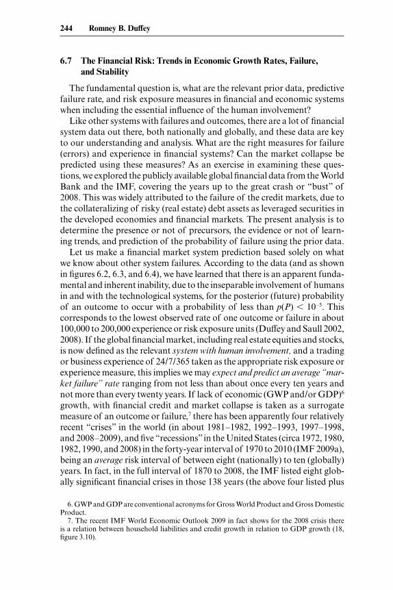
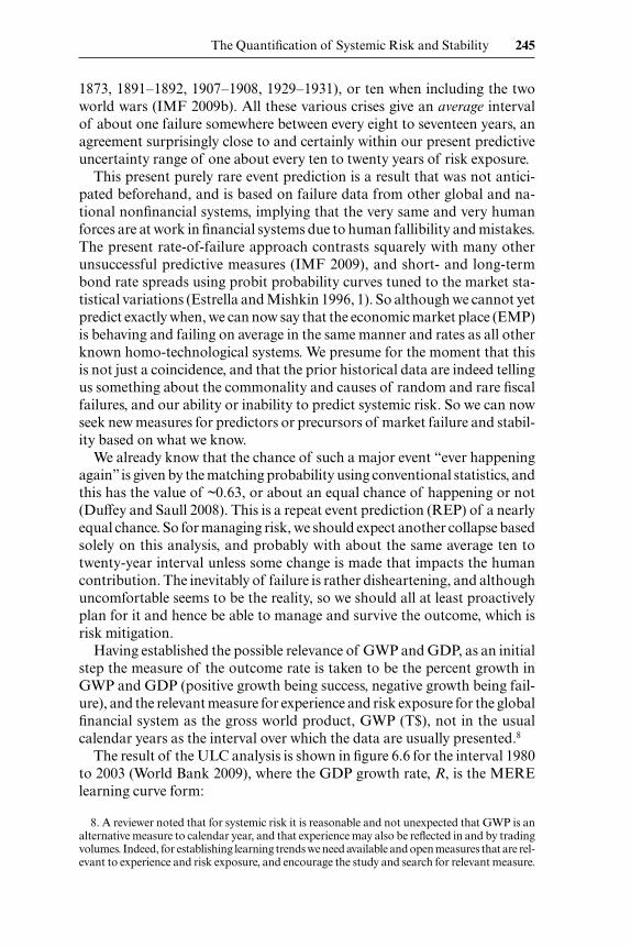
The result of the ULC analysis is shown in fi gure 6.6 for the interval 1980 to 2003 (World Bank 2009), where the GDP growth rate, R, is the MERE learning curve form:

8. A reviewer noted that for systemic risk it is reasonable and not unexpected that GWP is an alternative measure to calendar year, and that experience may also be refl ected in and by trading volumes. Indeed, for establishing learning trends we need available and open measures that are rel-evant to experience and risk exposure, and encourage the study and search for relevant measure.


R, %GWP � Rm � (R0 Rm) exp k(accGWP),

where numerically, from the data comparison in fi gure 6.6,

R � 0.08 � 8 exp

accGWP80

⎛⎝⎜

⎞⎠⎟.

The growth rate, R, is decreasing exponentially, and this expression is correlated with the data to an r2 � 0.9, and importantly shows that by a GWP of order $600T the overall global growth rate is trending toward being negligible (�0.1%).

In nondimensional form, relative to some initial growth rate, R0, this equa-tion can be written as:

R∗ �

RR0

�

1R0

⎛⎝⎜

⎞⎠⎟

0.08 + 8 exp − accGWP80

⎛⎝⎜

⎞⎠⎟

⎧⎨⎩

⎫⎬⎭

.

It is worth noting that, as might be expected in global trading, the magni-tude and growth of many economies are apparently highly correlated with the accumulated GWP, so will follow similar trends, as we see later. For ex-ample, the straight line that gives the relation between the US GDP and the GWP for the interval 1981 to 2004 is:

GDP(USA, $B) � 15{accGWP($T)} � 3,210,

with a correlation coefficient of r2 � 0.99. The magnitudes are hence very tightly coupled; but here we do not have to decide which is cause and which is effect (i.e., is the change in one due to the other, or vice versa?).9

To be clear, we really wish to determine a global fi nancial failure rate and

Fig. 6.6 The GWP growth rate curve

9. As pointed out by one of the discussers of this chapter, the “tight coupling” condition is one of those qualities proposed for the occurrence of so- called “normal accidents” (Perrow 1984).


the rate we are learning. So what is the relevant measure of the failure rate? Now, global governments and economies usually aim for increasing, or more slowly declining and hopefully nonnegative, growth. We postulate that either of the following extremes can be taken as an equivalent and immediately use-ful measure of economic failure, both varying with increasing accumulated GWP as a measure of total risk exposure: (a) the rate of decline in GWP growth rate; or (b) the rate of GWP growth rate itself.

By straightforward differentiation of the growth rate, R, we have the global failure or decline rate, �f, given by:

�f �

dRdGWP

� k(R0 Rm)exp k(accGWP).

Thus, numerically, we may expect the rate of decline of growth (the global fi nancial failure rate) to decrease with increasing risk exposure and experi-ence and be given very nearly by, in units of percent / GWP:

�f � 0.1 exp

accGWP80

⎛⎝⎜

⎞⎠⎟,

with the natural limit, �0 � 0.1, so the relevant nondimensional equation is,

E∗ �

� f

�0

� exp

accGWP80

⎛⎝⎜

⎞⎠⎟.

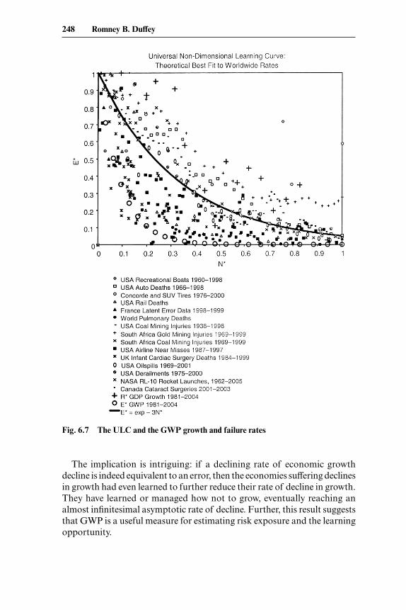
The equations for R∗ and E∗ now allow a direct comparison to the sys-temic learning trends given by the ULC form, E∗ � exp – 3N∗, so we also plotted these two growth decline predictions (shown as the large crosses and circles)10 in nondimensional form against all other world outcome data with the result shown in fi gure 6.7. The data are bracketed by the two extreme assumptions, basically: (a) the rate of decline of growth rate, �f , when equiv-alent to fi nancial failure, is tracking somewhat below other adverse outcome data; while (b) the simple decline in growth rate R is somewhat above other adverse data. We can indeed establish and cover the range with these two failure measures, generally within the data scatter.

To our knowledge this is the fi rst time that fi nancial and economic systems have been compared to other modern systems. We take the extraordinary fact that we can bring all these apparently disparate data together using the learning theory as evidence that the human involvement is dominant, not just in accidents and surgeries but also in economics, through the common basis of the fundamental decision and learning processes. Globally, there-fore, we can state that we have indeed learned to reduce and manage the rate of overall economic decline, just as we have learned to correct errors and failures in other systems.

10. This graph and comparison now responds to a point arising in the discussion at the fi rst draft presentation of this chapter as to the relevant measure for failure in global systems that exhibit varying growth rates.


The implication is intriguing: if a declining rate of economic growth decline is indeed equivalent to an error, then the economies suffering declines in growth had even learned to further reduce their rate of decline in growth. They have learned or managed how not to grow, eventually reaching an almost infi nitesimal asymptotic rate of decline. Further, this result suggests that GWP is a useful measure for estimating risk exposure and the learning opportunity.

Fig. 6.7 The ULC and the GWP growth and failure rates


6.8 Developing and Developed Economies: The Learning Link

It has been suggested that this decline in growth rate represents saturation of the developed economies, and that major growth then only occurs in the developing economies. To compare growth rates, the IMF and World Bank have also separated out the percentage GDP growth rates for “emerging” or developing countries / economies from “developed” or “advanced” coun-tries / economies (World Bank 2009).

Now the percentage growths are based on very different totals, so just for a comparison exercise, the percent growth rate, �GR, in each grouping was defi ned relative to the absolute growth in the world, or GWP, as:

�GR

%$T

⎛⎝⎜

⎞⎠⎟

�

% GDP Growth(GWP $T × World % Growth)

.

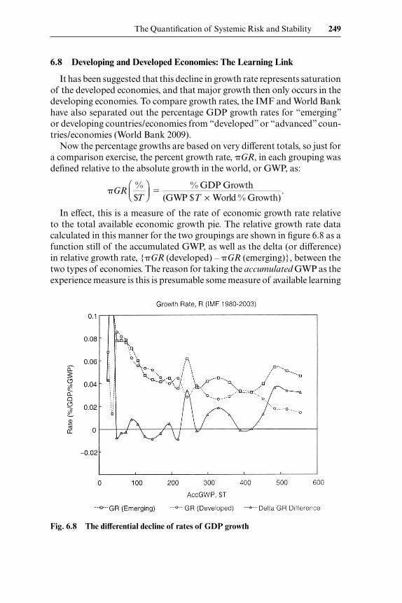
In effect, this is a measure of the rate of economic growth rate relative to the total available economic growth pie. The relative growth rate data calculated in this manner for the two groupings are shown in fi gure 6.8 as a function still of the accumulated GWP, as well as the delta (or difference) in relative growth rate, {�GR (developed) – �GR (emerging)}, between the two types of economies. The reason for taking the accumulated GWP as the experience measure is this is presumable some measure of available learning

Fig. 6.8 The differential decline of rates of GDP growth


experience and risk exposure in the global trade between the two groups, and of the total available pie.

What is seen is illuminating: the two growth rates (top dashed lines) are in antiphase or negatively correlated: when one goes up, the other goes down, and vice versa. One grows literally at the expense of the other. There is also some periodicity in the divergence pattern, and evidence of emerging positive divergence in growth rates toward $600T in 2003�. The opposite correlation between the growth rates is clear—the developing economies have a positive correlation of ~�0.9 and the developed economies a nega-tive correlation of about –0.7, with increasing accumulated GWP. As world wealth increases, one is declining, and the other is increasing in growth rate. The implication is that the relative growth shares part of the global economy pie growth, and hence the economies themselves are indeed closely coupled, which is perhaps obvious in hindsight.

The prediction is clear based on these trends. The developed world econo-mies would actually go into near zero or into negative GDP growth rate in 2003� (the projection is around 2005 to 2006 when GWP exceeds $600T), after many years of decline. The emerging economies would continue to grow positively at 5 percent or more. The difference in rates was highly oscil-latory and perhaps not stable, as the liquidity (credit) needed to fund growth in emerging economies cannot come from those developed economies whose available assets and economies are in decline. So the implication is that—in a globalized economy where all the individual economies are linked or “tightly coupled”—there are unknown feedback and stability relationships at work that we need to examine.

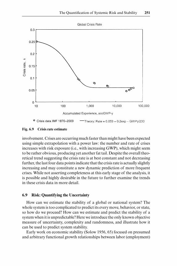
A very fi rst attempt was also made to predict the actual rate of the known global fi scal crises, where the key is again fi nding the relevant units for the measure of the risk exposure / experience, �. For the preliminary results shown in fi gure 6.9, as listed in the IMF’s WEO2009, the experience was taken as GWP- years for the interval 1870 to 2009, with eight nonwartime crises. The resulting global crisis rate, �G, is

�G � (Number of crises, per accumulated risk exposure years from 1870,

accY ).

The theory line also shown in fi gure 6.9 is derived from a MERE failure rate, which is fi rmly based on human learning, so that the equation is:

�G � 0.059 � 0.2 exp –

accGWPy230

⎛⎝⎜

⎞⎠⎟,

with a correlation of r2 � 0.958.Clearly the predicted tail is nearly constant with the lowest presently

attainable crisis rate of about 0.06 per year (or averaging one every seven-teen years), suggesting a plateau in the fi nite minimum rate due to human


involvement. Crises are occurring much faster than might have been expected using simple extrapolation with a power law: the number and rate of crises increases with risk exposure (i.e., with increasing GWP), which might seem to be rather obvious, producing yet another fat tail. Despite the overall theo-retical trend suggesting the crisis rate is at best constant and not decreasing further, the last four data points indicate that the crisis rate is actually slightly increasing and may constitute a new dynamic prediction of more frequent crises. While not asserting completeness at this early stage of the analysis, it is possible and highly desirable in the future to further examine the trends in these crisis data in more detail.

6.9 Risk: Quantifying the Uncertainty

How can we estimate the stability of a global or national system? The whole system is too complicated to predict its every move, behavior, or state, so how do we proceed? How can we estimate and predict the stability of a system when it is unpredictable? Here we introduce the only known objective measure of uncertainty, complexity and randomness, and illustrate how it can be used to predict system stability.

Early work on economic stability (Solow 1956, 65) focused on presumed and arbitrary functional growth relationships between labor (employment)

Fig. 6.9 Crisis rate estimate


and wealth generation (capital) for determining equilibrium conditions.11 The actual form of the economic growth function was not given or known, but using simple analytical functions, the possibility was shown for the exis-tence of multiple alternate steady- states or equilibria. But as clearly stated by Soros (2009): “The fi nancial system is far from equilibrium. . . . The short term needs are the opposite of what is needed in the long term.”

Since fi nancial markets are actually unstable and dynamic and not in equi-librium, the real need is to determine and predict the instant of and condi-tions for instability, not whether some ideal equlilibria or new steady state is achievable. Markets just like the entire physical world are random, chaotic, and unpredictable, so predicting frequent and rare events is risky and uncer-tain.12 Learning and randomness are powerful and unpredictable issues for risk prediction because we tend to believe that things behave according to what we know and, consciously or unconsciously, dismiss the risk of what we have not seen or do not know about. After all, we do not know what we do not know. We, as humans, are the very product of our norms and patterns, our knowledge skills and experience, our learning patterns and neural con-nections, our social milieu and moral teachings, in the jobs, friends, lovers, lives, teachers, family, and managers we happen to have. We perceive our own risk based on what we think we know, rightly or wrongly, and what we have experienced. But in key innovations and new disciplines, where knowledge and skill is still emerging—areas like terrorism, bio engineering, neuroscience, medicine, economics, computing, automation, genetics, law, space exploration, and nuclear reactor safety—we have to know and to learn the risk of what we know about what we do not know. We cannot possibly know everything, and these are all complex systems, with new and complex problems and lots of complexity, with much uncertainty.

The way to treat randomness and uncertainty has been solved in the physi-cal sciences, where it was realized that unobserved fl uctuations, uncertainty, and statistical fl uctuations govern and determine the actually observed behaviors and distributions. Events can happen or appear in many different ways, which is literally the “noise” that surrounds and confuses us, whereas what we actually observe is the most likely but also contains information about the signal that emerges or is embedded as order emerges from disor-der, and we process and discard the complexity. In fact, not just the physical world but the whole process of individual human response time and deci-sion making has been shown to be directly affected by randomness, in the so- called Hick- Hyman law (Duffey and Saull 2008). As individuals and as collectives, we do and must process complexity, both in our brains and in our behavior, seeking the signal from all the noise, the learning patterns from

11. The author is grateful to Ms. Christina Wang for pointing out both this reference and its relevance: for the present discussion we presume that “wealth creation” can be related or correlated to GWP and GDP.

12. The inherent randomness is often termed the aleatory uncertainty by statisticians.


the mistakes, and the information from all the distractions. Systematic pro-cessing and the perverse presence of complexity are essential for establishing learning distribution patterns.

The number of different ways something can appear or be ordered in sequence, magnitude, position, and experience, is mathematically derivable and is a measure of the degree of order in any system (Duffey and Saull 2008). The number of different ways is a measure of the complexity, and is determined by the Information Entropy, H, which is also a measure of what we know about what we do not know, or the “missing information” (Baierlein 1971), which is a measure of the risk. The relation linking the probability of any outcome to the entropy is well known from both Sta-tistical Physics and Information Theory, and is the objective measure of complexity:

Information Entropy, H � Sum( p � natural logarithm, p) � Σ p lnp.

Note that the units adopted or utilized for the entropy are fl exible and arbitrary, both by convention and in practice as being a comparative measure of order and complexity. So this measure of uncertainty requires a statement of probability. Now Taleb (2007, 315) noted that “I am purposely avoiding the notion of entropy because the way it is conventionally phrased makes it ill- adapted to the type of randomness we experience in real life.” We dismiss this assertion, and proceed to make this very subtle notion applicable to fi nancial systemic risk simply by rephrasing it.

To make the entropy concept adaptable and useful for “experience in real life,” all we have to do is actually relate and adapt the information entropy measure to our real life experience, or risk exposure interval, as we have already utilized (Duffey and Saull 2002, 2008) and have also introduced earlier. So we can now change the phrasing and the adaptability, since before we unconventionally phrase entropy as being “an objective measure of what we know about what we do not know, which is the risk.” In support of this use and phraseology, other major contributors have remarked:

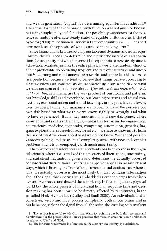
Entropy is defi ned as the amount of information about a system that is still unknown after one has made . . . measurements on the system. (Wolfram 2002, 44)

This suggests that . . . entropy might have an important place in guiding the strategy of a business man or stock market investor. (Jaynes 2003, 343 et seq.)

Entropy is a measure of the uncertainty and the uncertainty, or entropy, is taken as the measure of the amount of information conveyed by a message from a source.” (Pierce 1980, 23)

The uncertainty function . . . a unique measure for the predictability (uncertainty) of a random event which also can be used to compare diff-erent kinds of random events. (Greiner, Neise, and Stocker 1997, 150)


There is no other measure available or known with these fundamental properties and potential, particularly for handling uncertainty and random-ness, the processing and infl uence of complexity, and providing the objective measure of order. This measure also has direct application to the subjective concept of resilience engineering, where “resilience is the intrinsic ability of an organisation (system) to maintain or regain a dynamically stable state, which allows it to continue operation after a major mishap and / or the pres-ence of a continuous stress” (Hollnagel, Woods, and Leveson 2006, 9). But resilience, just like culture, has not been actually measured or quantifi ed any-where: it is simply a desirable property. We have developed the numerical and objective system organizational stability (SOS) criterion that incidentally unifi es the general theory and practice of managing risk through learning (Duffey and Saull 2008). This criterion is also relevant to crisis management policies and procedures, and emergency response centers in major corpora-tions, facilities, and industries.

6.10 System and Organizational Stability: SOS

The function of any management system is to create order from disorder, be it safety, regulatory, organizational, or fi nancial and hence to reduce the entropy. Thus, for order to emerge from chaos, and for stability in physical systems, the incremental change in entropy, which is the measure of the disorder, must be negative (Kondepudi and Prigogine 1998). Our equiva-lent SOS criterion or indicator then arises implying from the fact that the incremental change in risk (information entropy, H) with changes in prob-ability must be negative, or decreasing with increasing risk exposure. In any experience increment we must have the inequality, expressed in differential form to refl ect dynamic change:

dHd�

� 0.

Stated in words, for fi nancial systems and markets, this SOS criterion states that there must be an incremental decrease in complexity with increasing or changing risk exposure. Conversely, increasing complexity with incremental risk exposure is systemically unstable.

This key condition or indicator also requires that a maximum (peak) exists in our changing missing information or state of order as a function of experience and / or risk exposure, equivalent to a meta- stable condition. To illustrate this variation, consider the limit cases of concern of the prob-ability / possibility / likelihood of another collapse event, having observed a similar one already, considering all our previous knowledge. From the past experience we showed that the prior probability for REP is, with little learn-ing, p ≈ (1 – 1 / e) � 0.63, and also this same value holds for novice mistakes with little experience (when �0). For the future risk, the posterior probability,


with little learning, is p ≈ 1 / � for rare events and also for highly experienced systems (when � → �).

For the two limited learning cases of the prior (past MERE) and posterior (future rare event) the entropy increment, dH � –plnp in any risk interval can be calculated. The results are shown in fi gure 6.10 as a function of the experience or risk exposure interval, N∗, which purely for convenience has been nondimensionalized to the maximum experience or risk exposure. For the example known prior case, entropy is calculated from the MERE prob-ability result with little learning (k � 0.0001); the decrease in entropy at larger experience or risk exposure for the prior case is due to the probability of an outcome fi nally reaching a certainty, p ~ 1, as ultimately there is no uncertainty. For the unknown posterior case, the entropy is calculated from p � 1 / �; the peak in entropy at small experience is simply due to the greater uncertainty, which decreases as experience is gained.

Also shown in the fi gure 6.10 is the purely theoretical prediction obtained from SEST, the statistical error state theory (Duffey and Saull 2008), which treats outcomes as appearing randomly. The theory derives the most likely statistical distribution of outcomes, and relates the probability of the out-comes with variation in the instantaneous depth of experience or risk expo-sure in any given risk interval. The information entropy, H, is the measure of the complexity in any interval and is given by integrating the resulting exponential probability distributions, to obtain:

Fig. 6.10 Entropy variations with experience, knowledge, and risk exposure: Sta-bility indicator


H �

12

( p0 exp aN∗)2

aN∗ + 12

⎛⎝⎜

⎞⎠⎟

.

At small experience, as N∗ → 0, the previous SEST result becomes H → 0.25, which is close to the prior value with little learning of H → 0.29, so the two results are also consistent in their limits, as they should be. The value of the slope parameter or learning exponent, a, is derived deliberately from very diverse prior data sets for failure distributions, which are very detailed and complete.13 The theory line in fi gure 6.10 utilizes the “best” a � 3.5 in the earlier exponential distribution as a working approximate estimate for com-parison purposes, which is close to the learning rate constant value, k ~ 3. For most of the experience or risk range shown, the entropy is not decreasing signifi cantly until sufficient experience is attained.

Figure 6.10 itself contains information about what we know about what we do not know, so is worth some more discussion. Knowns (prior or past) apparently contain more uncertainty (H is larger) than unknowns (posterior or future), except at very early or little experience (N∗ � 10–4). The shapes of the curves are of interest for another reason: for evaluating the system organizational stability (SOS) criterion. By inspection of the two cases in fi gure 6.10, this stability condition is only met or satisfi ed at small experience for the unknowns, and at large experience for the knowns.

Basically, at small experience unless learning is occurring the existing sys-tem is unstable and in danger of repeat events until very large experience is attained. Conversely, any future system is also initially unstable until sufficient post- entry experience has been attained. So learning—or decreasing com-plexity—is essential for stability, and this is plainly relevant to the market sta-bility when introducing the use of new and / or complex fi nancial instruments.

Quoted at the very beginning of this chapter, we can now return to the statement in Soros (2009) that “markets are unstable,” a controversial assertion when contrasted with normal economic theory based on near- equilibrium markets (the balance between supply and demand as refl ected in price). To test this assertion, the data points shown as circles in fi gure 6.10 are for the trial crisis entropy estimates calculated using the preliminary prob-ability values for rare events, p ≈ n / accGWP, where n is simply the number of observed crises, and the risk interval or experience has been nondimen-sionalized on the basis of the accumulated GWP from 1870 to 2009. The general data trend is downward (i.e., stable) until the last few data points for the crises of 1997 and 2007. Moreover, the greater the GWP becomes, the greater the risk. Importantly, the slope of the last four data points being positive satisfi es the formal indicator (the criterion dH / d� � 0) for inherent global market instability, as has been previously suggested (Soros 2009).

13. Specifi cally, we used: (a) US commercial aircraft near midair collisions (NMACs) for 1987 to 1998, where experience and risk exposure is measured by total fl ights; and (b) Australian traffic fatalities from 1980 to 1999, where experience and risk exposure is measured in driver- years (as shown in 5, fi gure 8.8).


The present results and stability indicator are based on the inclusion of the uncertainty due to human decision making and risk taking, and thus quan-tifi es and supports the idea independently and effectively simultaneously proposed by Soros (2010) of the Human Uncertainty Principle.14 This prin-ciple is fi rmly based on experience and learning from investment and market behaviors, and proposes that human involvement and risk taking inherently introduces risk due to incomplete knowledge and complexity, resulting in intervention actions in the market based on imperfect understanding that have unintended consequences, in what Soros describes as “refl exivity.”

This new data comparison suggests that entropy is indeed a potentially signifi cant indicator that should not be simply avoided as Taleb does, and represents our best and most refi ned state of knowledge regarding systemic risk. We have now actually quantifi ed the behavior of the chaotic and random fi nancial market. As to regulation of systemic risk, this is really about regulat-ing such unknown uncertainty while meeting the stated goals (Brown 2009; RECP 2008). In fact, Brown (2009, 209) suggests that “to be effective and worthy of public trust, any governance system must be able to demonstrate technical competence. Effective and trustworthy governance arrangements must have four key qualities: informed, transparent, prospective and adap-tive.” We have provided new technically- founded measures for the basis of a governance system that are: (a) informed by the actual world data and vali-dated; (b) transparent both in their calculation and in using the precepts that describe human learning and risk taking; (c) prospective and future orien-tated by being able to make actual predictions; and (d) adaptive to generally encompass changes in chaotic markets, risk exposure, and fi nancial systems.

6.11 Concluding Remarks: Our New Methods and Measures Provide This Framework for Objective and Predictive Governance

An exercise such as predicting the next recession or crisis becomes simply equivalent to determining the probability of and risk interval for the next event or outcome. This probability must be based on relevant and correlated measures for experience and risk exposure, which include the presence or absence of learning. We have analyzed the world economic data to make a prediction of the next crisis probability based on the presence and infl uence of human risk taking and decision making in fi nancial markets.15

We have summarized some recent ideas on risk prediction for multiple tech-nological systems, using the existing data, and have explicitly included the key

14. By delightful chance, within a week of each other on two continents, the verbal Soros “Lec-tures” were given on October 26–30, 2009, in Budapest, and the present chapter presented at the NBER Research Conference on Quantifying Systemic Risk on November 6, 2009, in Cambridge.

15. In response to a question raised in discussion at the conference, the present estimate and prediction based on past data is for one global fi nancial crisis occurring at least every eight to seventeen years, becoming more frequent in the future as the GWP and concomitant risk exposure grow. Knowing this fact, the keys are to be prepared for crisis and proactive in risk management.


impact of human involvement using the learning hypothesis, namely that we learn from our mistakes. This ability of homo- technological systems to learn from experience reduces risk and errors, but also produces a fat tail as the processes of learning, making errors, and risk taking persist. We have related these ideas to the prediction of rare events, systemic risk, and organizational stability in global systems and, although we do not pretend to have all the answers, there are clear directions to follow. Risk is caused by our uncertainty, and the measure of uncertainty is probability. The risk of an outcome (acci-dent, event, error, or failure) is never zero, and the possibility of an outcome always exists, with a chance given by the future (posterior) probability. The key is to include the human involvement, and to create and use the correct and relevant measures for experience, learning, complexity, and risk exposure.

Standard statistical distributions and indicators presently used for fi nancial systems (e.g., as used in VaR, or yield spread) are known to not be applicable for predicting rare events, systemic risk, crises, and failures. Because of the human involvement, the risk becomes greater than just by using a Gaussian, normal, or simple power law, until we reach very, very large experience and would have had a prior event anyway. We have a greater chance of outcomes and unexpected unknown unknowns if we are not learning than we might expect even from and if using simple scaling or power laws. This is simply because we are humans who make mistakes, take risks, and cannot be error- free. In colloquial terms, the human adds another fat tail to an already fat tail.

So the past or prior knowledge indeed informs the future risk: what we know from what we already know from the probability of what were once past unknowns tells us about the probability of the unknown unknowns in the future also.

The measure adopted and used and that is relevant for estimating risk exposure is key. Over some seven to eight decades (orders of magnitude) variation in the rate and in the risk exposure or accumulated experience, for the rare event the negligible learning prediction holds. At any future experience or risk exposure, the error (or uncertainty) in the risk prediction is evidently about a factor of ten in future crisis occurrence probability, and about a factor of two in average crisis frequency.

We have suggested several major factors and useful measures that infl u-ence the prediction of risk and stability in fi nancial systems, based on what we observe for all other systems with human involvement:

1. The Universal Learning Curve provides a comparative indication of trends.

2. The probability of failure / loss is a function of experience or risk expo-sure.

3. The relevant measure of failure is the rate of decline in GDP growth rates.

4. A relevant measure of experience and risk exposure is the accumulated GWP.


5. Stable systems are learning systems that reduce complexity.6. An absolute measure of risk and uncertainty is the Information

Entropy, which refl ects what we know about what we do not know.7. Unique conditions exist for systemic stability.8. Repeat events are likely.9. Existing systems are unstable unless learning occurs.10. New systems are unstable at small experience.

The rare events are essentially all the same, whether they be aircraft crashes, space shuttle losses, massive explosions, or huge fi nancial crises: we know nothing about them until they actually happen, when and if they occur almost magically becoming known unknowns. We learn from them only after they have happened at least once. But based on what we know about what we do not know, we can always estimate our risk and whether we are learning or not. The rare unknown unknowns, or colloquially, the fat tails or Black Swans of the unpredictable rate distributions, are simple manifestations of the occurrence of these outcomes whenever and wherever they happen. We can and must expect them to continue to appear.

In our previous published work (Duffey and Saull 2008), we had quan-tifi ed the uncertainty or complexity using the information entropy, H, as an objective measure of other subjective organizational and management desiderata of safety culture and organizational learning as a function of experience. This is the fi rst time, to our knowledge, that information entropy has been introduced as an objective prediction of the subjective feeling of risk exposure in the presence or absence of learning. As to regulation of systemic risk, this is about regulating uncertainty, so that we demonstrate technical competence. We provide measures and indicators for the guidance of effective and trustworthy governance arrangements that possess the four key qualities of being informed, transparent, prospective, and adaptive.

The work and concepts discussed in this chapter are only a necessary fi rst step in developing understanding for predicting and managing risk in complex systems with human involvement. This new application to fi nan-cial systems and markets, and the adoption of new measures requires time, patience, and can also introduce risk. Further work is clearly needed in this whole arena of system stability, the selection of relevant experience mea-sures, and the quantifi cation and prediction of future risk.

Appendix

Probability Defi nition

The outcome probability is just the cumulative distribution function (CDF) conventionally written as F(�), the fraction that fails by �, so:


p(�) � F(�) � 1 exp ∫ �dt,

where the failure rate:

�(�) � h(�) �

f (�)R(�)

�

1(1 − F)

⎧⎨⎩

⎫⎬⎭

dFd�

, and the p.d.f. f(�) � dF / d�.

Carrying out the integration from an initial experience to any interval �, we obtain the probability of an outcome as the double exponential:

p(�) � 1 exp

(� − �m)(k − �m�)

⎧⎨⎩

⎫⎬⎭

where, from integrating the minimum error rate equation (MERE), (d� / d�) � –k(� – �m), the failure rate is:

�(�) � �m � (�0 �m) exp k�

and �(�0) � �0 at the initial experience, accumulated up to or at the initial outcome(s), and �0 � 1 / � for the very fi rst, rare, or initial outcome, like an inverse power law.

In the usual engineering reliability terminology, for n failures out of N total, the failure probability,

p(�) � (1 R(�)) �

# failurestotal number

�

nN

,

and the frequency is known if, n and N are known (and generally N is not known).

References

Baierlein, R. 1971. Atoms and Information Theory: An Introduction to Statistical Mechanics. New York: Dover.

Barthelemy, F. 2001. Accident on the 21st of September 2001 at a Factory Belonging to the Grande Paroisse Company in Toulouse, Produced Jointly with the Explosives Inspectorate and with Help from the INERIS. Report of the General Inspectorate for the Environment, Affair no. IGE / 01 / 034. Paris: Inspection Générale de l’Environnement, October 24.

Bayes, Rev. T. 1763. “Memoir Communicated by R. Price, ‘An Essay Toward Solving a Problem in the Doctrine of Chances.’” Royal Society of London 53:376–98.

Brown, S. 2009. “The New Defi cit Model.” Nature Nanotechnology 4:609–11.Columbia Accident Investigation Board (CAIB). 2003. “Report, Volume 1.” August.

“Working Scenario.” July. CAIB / NASA / NAIT. http: // www.caib.us.Commission of Inquiry. 2007a. Report of the Commission of Inquiry into the Collapse

of a Portion of the de la Concorde Overpass. October. Gouvernement de Quebec. http: // www.cevc.gouv.qc.ca / UserFiles / File / Rapport / report_eng.pdf.

———. 2007b. Rapport sur les causes techniques de l’effondrement du viaduc de la Concorde. Principal report by Jacques Marchand and Denis Mitchell.


Coolen, F. P. A. 2006. “On Probabilistic Safety Assessment in the Case of Zero Failures.” Proceedings, Institution of Mechanical Engineers, Part O, J. Risk and Reliability 220 (2): 105–14.

Duffey, R. B. 2004. “Innovation in Technology for the Least Product Price and Cost—A New Minimum Cost Relation for Reductions during Technological Learning.” Int. J. Energy Technology and Policy 2 (1 / 2): 106–29.

Duffey, R. B., and T. S. Ha. 2009. “Predicting Electric Power System Restoration.” Paper presented at the Proc. IEEE (TIC- STH) Toronto International Confer-ence–Science and Technology for Humanity. Toronto, Ontario. September 27–29.

———. 2010. “Human Reliability: Benchmark and Prediction.” Proc. I. Mech. E, Part O: J. Risk and Reliability 224:186–96. doi: 10.1243 / 1748006XJRR307.

Duffey, R. B., and J. W. Saull. 2002. Know the Risk, 1st ed. Boston: Butterworth and Heinemann.

———. 2008. Managing Risk: The Human Element. West Sussex, UK: John Wiley & Sons Ltd.

Duffey, R. B., and A. B. Skjerve. 2008. “Risk Trends, Indicators and Learning Rates: A New Case Study of North Sea Oil and Gas.” Paper presented at the Proceedings of the European Safety and Reliability Conference (ESREL) 2008, 17th SRA Conference. Valencia, Spain. September 22–25.

Duffey, R. B., and R. L. Tapping. 2009. “Predicting Steam Generator Tube Fail-ures.” Paper presented at the Proceedings of the 6th CNS International Steam Generator Conference. Toronto, Ontario. November 8–11.

Estrella, A., and F. S. Mishkin. 1996. “The Yield Curve as a Predictor of US Reces-sions.” Current Issues in Economics and Finance 2 (7): 1–6. Federal Reserve Bank of New York.

Fragola, J. R. 2009. “How Safe Must a Potential Crewed Launcher be Demonstrated to be Before it is Crewed?” Journal of Loss Prevention in the Process Industries 22:657–63.

Greiner, W., L. Neise, and H. Stocker. 1997. Thermodynamics and Statistical Mechan-ics. New York: Springer.

Hanayasu, S., and K. Sekine. 2004. “Damage Assessment of Industrial Accidents by Frequency- Magnitude Curve.” Proceedings of Probabilistic Safety Assessment and Management (PSAM) 07, paper no. 0229.

Hollnagel, E., D. Woods, and N. Leveson, eds. 2006. Resilience Engineering: Con-cepts and Precepts. Hampshire, England: Ashgate Publishing Limited.

Holton, G. A. 2004. “Defi ning Risk.” Financial Analysts Journal 60 (6): 19–25. www.cfa.pubs.

Howlett, H. C. 2001. The Industrial Operator’s Handbook, 2nd ed. Pocatello, ID: Techstar.

International Monetary Fund (IMF). 2009a. “World Economic Outlook of the International Monetary Fund.” Update Table 1.1, January 28. www.IMF.org / external / pubs / ft / weo / 2009 / update. Washington, DC: IMF.

———. 2009b. “World Economic Outlook: Sustaining the Recovery.” Figure 3.1, October. Washington, DC: IMF.

Jaynes, E. T. 2003. Probability Theory: The Logic of Science, 1st ed. Cambridge: Cambridge University Press.

Kondepudi, D., and I. Prigogine. 1998. Modern Thermodynamics: From Heat Engines to Dissipative Structures. New York: John Wiley & Sons.

Ohlsson, S. 1996. “Learning From Performance Errors.” Psychological Review 103 (2): 241–62.

Perrow, C. 1984. Normal Accidents, Living with High Risk Technologies. New York: Basic Books.


Petroski, H. 1985. To Engineer Is Human: The Role of Failure in Successful Design. New York: St. Martin’s Press.

Pierce, J. R. 1980. An Introduction to Information Theory. New York: Dover.Royal Commission on Environmental Protection (RCEP). 2008. 27th Report:

“Novel Materials in the Environment: The Case of Nanotechnology.” Cm7468, HMSO. www.rcep.org.uk / reports.

Rumsfeld, Donald. 2002. US Defense Secretary, quoted from February 12th press conference. Available at http://en.wikipedia.org /wiki /.

Solow, R. M. 1956. “A Contribution to the Theory of Economic Growth.” Quarterly Journal of Economics 70 (1): 65–94.

Soros, G. 2009. “Do not ignore the need for fi nancial reform.” Financial Times, Com-ment section, October 26. www.ft.com / soros.

———. 2010. The Soros Lectures. Lecture One, Public Affairs. New York: Perseus Books Group.

Stevens, J. C., and H. B. Savin. 1962. “On the Form of Learning Curves.” J. Experi-mental Analysis of Behaviours 5 (1): 15–18.

Sveshnikov, A. A. 1968. Problems in Probability Theory, Mathematical Statistics and the Theory of Random Functions. New York: Dover.

Taleb, N. 2007. The Black Swan: The Impact of the Highly Improbable. New York: Random House.

US National Commission. 2011. Deep Water: The Gulf Oil Disaster and the Future of Offshore Drilling. Report to the President. Washington, DC: GPO.

US Nuclear Regulatory Commission (NRC). 2008. “Davis- Besse Reactor Pressure Vessel Head Degradation: Overview, Lessons Learned, and NRC Actions Based on Lessons Learned.” Report NUREG / BR- 0353, Rev. 1, August. www.nrc.gov.

Wolfram, S. 2002. A New Kind of Science. Champlain, IL: Wolfram Media, Inc.Woo, G. 1999. The Mathematics of Natural Catastrophes. London: Imperial College

Press.World Bank. 2009. “Gross World Product.” Available at www.- wds.worldbank

.org / WBSITE, GWP 1981–2004.

Comment Joseph G. Haubrich

In “The Quantifi cation of Systemic Risk and Stability: New Methods and Measures,” Romney B. Duffey reminds us that fi nancial markets are com-plex human systems, and argues that there is a lot to learn from failures in other complex human systems, such as airline fl ight, power generation, and cardiac surgery. Two key lessons that emerge are the importance of learn-ing and the proper measure of time. Learning has a somewhat paradoxical effect on failures: it is by experiencing failures that humans learn, and in turn adjust the system and create the techniques to prevent failures. This notion

Joseph G. Haubrich is a vice president of and an economist at the Federal Reserve Bank of Cleveland.

The views expressed here are those of the author only, and do not represent the views of the Federal Reserve Bank of Cleveland or the Board of Governors of the Federal Reserve System. For acknowledgments, sources of research support, and disclosure of the author’s material fi nancial relationships, if any, please see http: // www.nber.org / chapters / c12061.ack.

Documents

Quantifying Systemic Riskstock market crashes, the same learning principles also apply. We have shown We have shown that to quantify risk we must include the learning behavior, quantifying