Embed Size (px)
Citation preview

AFRL-RQ-WP-TR-2015-0069
QUANTIFYING CONFIDENCE IN MODEL PREDICTIONS FOR HYPERSONIC AIRCRAFT STRUCTURES Benjamin P. Smarslok Hypersonic Sciences Branch High Speed Systems Division MARCH 2015 Final Report
Approved for public release; distribution unlimited.
See additional restrictions described on inside pages
STINFO COPY
AIR FORCE RESEARCH LABORATORY AEROSPACE SYSTEMS DIRECTORATE
WRIGHT-PATTERSON AIR FORCE BASE, OH 45433-7541 AIR FORCE MATERIEL COMMAND
UNITED STATES AIR FORCE

NOTICE AND SIGNATURE PAGE
Using Government drawings, specifications, or other data included in this document for any purpose other than Government procurement does not in any way obligate the U.S. Government. The fact that the Government formulated or supplied the drawings, specifications, or other data does not license the holder or any other person or corporation; or convey any rights or permission to manufacture, use, or sell any patented invention that may relate to them. This report was cleared for public release by the USAF 88th Air Base Wing (88 ABW) Public Affairs Office (PAO) and is available to the general public, including foreign nationals. Copies may be obtained from the Defense Technical Information Center (DTIC) (http://www.dtic.mil). AFRL-RQ-WP-TR-2015-0069 HAS BEEN REVIEWED AND IS APPROVED FOR PUBLICATION IN ACCORDANCE WITH ASSIGNED DISTRIBUTION STATEMENT. *//Signature// //Signature// BENJAMIN P. SMARSLOK MEI-LING LIBER, Branch Chief Program Manager Hypersonic Sciences Branch Hypersonic Sciences Branch High Speed Systems Division High Speed Systems Division //Signature// THOMAS A. JACKSON, Deputy for Science High Speed Systems Division Aerospace Systems Directorate This report is published in the interest of scientific and technical information exchange, and its publication does not constitute the Government’s approval or disapproval of its ideas or findings. *Disseminated copies will show “//Signature//” stamped or typed above the signature blocks.

REPORT DOCUMENTATION PAGE Form Approved OMB No. 0704-0188
The public reporting burden for this collection of information is estimated to average 1 hour per response, including the time for reviewing instructions, searching existing data sources, searching existing data sources, gathering and maintaining the data needed, and completing and reviewing the collection of information. Send comments regarding this burden estimate or any other aspect of this collection of information, including suggestions for reducing this burden, to Department of Defense, Washington Headquarters Services, Directorate for Information Operations and Reports (0704-0188), 1215 Jefferson Davis Highway, Suite 1204, Arlington, VA 22202-4302. Respondents should be aware that notwithstanding any other provision of law, no person shall be subject to any penalty for failing to comply with a collection of information if it does not display a currently valid OMB control number. PLEASE DO NOT RETURN YOUR FORM TO THE ABOVE ADDRESS.
1. REPORT DATE (DD-MM-YY) 2. REPORT TYPE 3. DATES COVERED (From - To)March 2015 Final 01 October 2011 – 30 September 2014
4. TITLE AND SUBTITLEQUANTIFYING CONFIDENCE IN MODEL PREDICTIONS FOR HYPERSONIC AIRCRAFT STRUCTURES
5a. CONTRACT NUMBER In-house
5b. GRANT NUMBER
5c. PROGRAM ELEMENT NUMBER 61102F
6. AUTHOR(S)
Benjamin P. Smarslok 5d. PROJECT NUMBER
3002 5e. TASK NUMBER
N/A 5f. WORK UNIT NUMBER
Q184 7. PERFORMING ORGANIZATION NAME(S) AND ADDRESS(ES) 8. PERFORMING ORGANIZATION
Hypersonic Sciences Branch (AFRL/RQHF) High Speed Systems Division Air Force Research Laboratory, Aerospace Systems Directorate Wright-Patterson Air Force Base, OH 45433-7541 Air Force Materiel Command, United States Air Force
REPORT NUMBER
AFRL-RQ-WP-TR-2015-0069
9. SPONSORING/MONITORING AGENCY NAME(S) AND ADDRESS(ES) 10. SPONSORING/MONITORINGAir Force Research Laboratory Aerospace Systems Directorate Wright-Patterson Air Force Base, OH 45433-7541 Air Force Materiel Command United States Air Force
AGENCY ACRONYM(S)AFRL/RQHF
11. SPONSORING/MONITORINGAGENCY REPORT NUMBER(S)
AFRL-RQ-WP-TR-2015-0069 12. DISTRIBUTION/AVAILABILITY STATEMENT
Approved for public release; distribution unlimited.13. SUPPLEMENTARY NOTES
PA Case Number: 88ABW-2015-1227; Clearance Date: 18 Mar 2015.14. ABSTRACT
Lack of confidence in structural response and life predictions of a vehicle exposed to combined extreme environmentshas consistently prevented the USAF from fielding affordable, reliable, and reusable hypersonic space access platforms.Significant strides have been made in modeling complex interactions of the multi-physics, fluid-thermal-structuralcoupling applicable to hypersonic flow conditions. However, validation of these models remains a challenge due tolimited experimental data for hypersonic conditions. This research addresses fundamental and critical issues inquantifying uncertainty and assessing the confidence in model predictions of hypersonic structural response through asystematic framework.
15. SUBJECT TERMSuncertainty quantification, Validation, Bayesian techniques
16. SECURITY CLASSIFICATION OF: 17. LIMITATIONOF ABSTRACT:
SAR
18. NUMBEROF PAGES
122
19a. NAME OF RESPONSIBLE PERSON (Monitor) a. REPORT Unclassified
b. ABSTRACTUnclassified
c. THIS PAGEUnclassified
Benjamin P. Smarslok 19b. TELEPHONE NUMBER (Include Area Code)
N/A Standard Form 298 (Rev. 8-98) Prescribed by ANSI Std. Z39-18
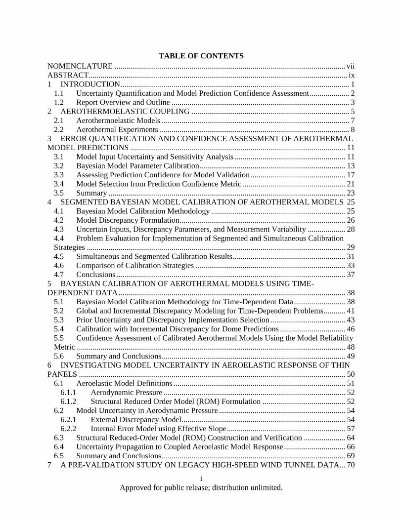
TABLE OF CONTENTS NOMENCLATURE ..................................................................................................................... vii ABSTRACT ................................................................................................................................... ix 1 INTRODUCTION .................................................................................................................... 1
1.1 Uncertainty Quantification and Model Prediction Confidence Assessment .................... 2 1.2 Report Overview and Outline .......................................................................................... 3
2 AEROTHERMOELASTIC COUPLING ................................................................................ 5 2.1 Aerothermoelastic Models ............................................................................................... 7 2.2 Aerothermal Experiments ................................................................................................ 8
3 ERROR QUANTIFICATION AND CONFIDENCE ASSESSMENT OF AEROTHERMAL MODEL PREDICTIONS ............................................................................................................. 11
3.1 Model Input Uncertainty and Sensitivity Analysis ........................................................ 11 3.2 Bayesian Model Parameter Calibration.......................................................................... 13 3.3 Assessing Prediction Confidence for Model Validation ................................................ 17 3.4 Model Selection from Prediction Confidence Metric .................................................... 21 3.5 Summary ........................................................................................................................ 23
4 SEGMENTED BAYESIAN MODEL CALIBRATION OF AEROTHERMAL MODELS 25 4.1 Bayesian Model Calibration Methodology .................................................................... 25 4.2 Model Discrepancy Formulation .................................................................................... 26 4.3 Uncertain Inputs, Discrepancy Parameters, and Measurement Variability ................... 28 4.4 Problem Evaluation for Implementation of Segmented and Simultaneous Calibration Strategies ................................................................................................................................... 29 4.5 Simultaneous and Segmented Calibration Results ......................................................... 31 4.6 Comparison of Calibration Strategies ............................................................................ 33 4.7 Conclusions .................................................................................................................... 37
5 BAYESIAN CALIBRATION OF AEROTHERMAL MODELS USING TIME-DEPENDENT DATA ................................................................................................................... 38
5.1 Bayesian Model Calibration Methodology for Time-Dependent Data .......................... 38 5.2 Global and Incremental Discrepancy Modeling for Time-Dependent Problems ........... 41 5.3 Prior Uncertainty and Discrepancy Implementation Selection ...................................... 43 5.4 Calibration with Incremental Discrepancy for Dome Predictions ................................. 46 5.5 Confidence Assessment of Calibrated Aerothermal Models Using the Model Reliability Metric ........................................................................................................................................ 48 5.6 Summary and Conclusions ............................................................................................. 49
6 INVESTIGATING MODEL UNCERTAINTY IN AEROELASTIC RESPONSE OF THIN PANELS ....................................................................................................................................... 50
6.1 Aeroelastic Model Definitions ....................................................................................... 51 6.1.1 Aerodynamic Pressure ............................................................................................ 52 6.1.2 Structural Reduced Order Model (ROM) Formulation .......................................... 52
6.2 Model Uncertainty in Aerodynamic Pressure ................................................................ 54 6.2.1 External Discrepancy Model ................................................................................... 54 6.2.2 Internal Error Model using Effective Slope ............................................................ 57
6.3 Structural Reduced-Order Model (ROM) Construction and Verification ..................... 64 6.4 Uncertainty Propagation to Coupled Aeroelastic Model Response ............................... 66 6.5 Summary and Conclusions ............................................................................................. 69
7 A PRE-VALIDATION STUDY ON LEGACY HIGH-SPEED WIND TUNNEL DATA... 70
i Approved for public release; distribution unlimited.
7.1 Legacy Aerothermal Data from the NASA High-Temperature Tunnel ............................. 70 7.2 Mathematical Methods .................................................................................................... 72
7.2.1 Posterior p-Value ...................................................................................................... 72 7.2.2 Metropolis-Hastings Algorithm ................................................................................ 74 7.2.3 U-pool Defect .......................................................................................................... 75 7.2.4 Confidence Structure on the Non-Parametric Difference ......................................... 76
7.3 Data and Models ............................................................................................................. 76 7.3.1 Pre-shock Conditions ................................................................................................ 77 7.3.2 No-Bias Hypothesis ................................................................................................ 78 7.3.3 Free Stream Bias ..................................................................................................... 78 7.3.4 Deflection Bias Hypothesis..................................................................................... 79 7.3.5 Dome Pressure Asymmetry .................................................................................... 79
7.4 Results ............................................................................................................................ 79 7.4.1 Pressure Ratio Bias ................................................................................................. 79 7.4.2 Pressure Tap Asymmetry ........................................................................................ 80
7.5 Conclusions and Future Work ........................................................................................ 81 8 UNCERTAINTY QUANTIFICATION OF STATE BOUNDARIES IN THIN BEAM BUCKLING EXPERIMENTS ..................................................................................................... 83
8.1 Physical Example: Thin Beam Buckling Temperature .................................................. 84 8.2 Methodology for State Boundary Uncertainty Quantification ....................................... 86
8.2.1 Probabilistic Model Selection ................................................................................. 87 8.2.2 Bayesian Network Formulation of Probabilistic Model Selection ......................... 88 8.2.3 Handling Uncertainty in Training Data Near the Boundary ................................... 89 8.2.4 Quantification of State Boundary Uncertainty ....................................................... 92 8.2.5 Methodology Summary .......................................................................................... 92
8.3 Case Study: Thin Beam Buckling .................................................................................. 92 8.3.1 Experimental Procedure .......................................................................................... 92 8.3.2 Uncertainty in Buckling Temperature Identification .............................................. 93 8.3.3 Experimental Data .................................................................................................. 93 8.3.4 Bayesian Network and SBUQ ................................................................................ 94 8.3.5 Results and Discussion ........................................................................................... 97
8.4 Summary of State Boundary Uncertainty Quantification .............................................. 98 9 REFERENCES ....................................................................................................................... 99
ii Approved for public release; distribution unlimited.
LIST OF FIGURES Figure Page Figure 1.1. Framework for integrating of models, data, and uncertainty ...................................... 3 Figure 2.1. Representative hypersonic vehicle structure with aerothermoelastic panel [11] ........ 5 Figure 2.2. Coupling in aerothermoelasticity ................................................................................ 6 Figure 2.3. Instrumentation locations on spherical dome geometry [44] ...................................... 9 Figure 2.4. Estimated transient temperature distributions from Runs 30, 31, and 32 ................. 10 Figure 3.1. Bayesian network for calibrating model inputs and errors using aerothermal data . 14 Figure 3.2. Prior and posterior distributions for a) freestream temperature T1, and b) wall
temperature Tw4 ...................................................................................................... 15 Figure 3.3. Prior and posterior distributions for a) error in flat plate p4, b) error in flat plate
Q4, c) error in spherical dome p4, and d) error in spherical dome Q4 .................... 16 Figure 3.4. Aerodynamic pressure along centerline of spherical dome for Runs 30, 31, and 32
from test data, initial mean input values, and Bayesian updated mean input values 17 Figure 3.5. Aerodynamic heat flux along centerline of spherical dome for Runs 30, 31, and 32
from experimental data, initial mean input values, and Bayesian updated mean input values .............................................................................................................. 18
Figure 3.6. Aerodynamic pressure predictions for Run 30 using 1st-,2nd-, and 3rd-order piston theory ....................................................................................................................... 22
Figure 3.7. Aerodynamic heat flux predictions for Run 30 using 1st-,2nd-, and 3rd-order piston theory............................................................................................................. 22
Figure 4.1. Bayesian Network for Glass and Hunt experiments................................................... 26 Figure 4.2. Aerodynamic pressure predictions across dome at nominal input values .................. 27 Figure 4.3. Aerodynamic heat flux predictions across dome at nominal input values ................. 27 Figure 4.4. Prior and posterior distributions for a) freestream temperature and b) wall
temperature .............................................................................................................. 31 Figure 4.5. Prior and posterior distributions for (a) oblique shock error, (b)-(d) piston theory
error and, (e)-(g) Eckert's reference temperature error ............................................ 32 Figure 4.6. Prior and posterior distributions for (a) pressure and (b) heat flux measurement
error .......................................................................................................................... 32 Figure 4.7. Pressure predictions across dome from posterior distributions .................................. 35 Figure 4.8. Heat flux predictions across dome from posterior distributions ................................ 36 Figure 5.1. Aerothermal Bayesian Network for Glass and Hunt experiments ............................. 39 Figure 5.2. Bayesian Network with Time-Dependent Data for Aerothermal Coupling .............. 39 Figure 5.3. Nominal aerothermal temperature prediction compared to midpoint data ................. 40 Figure 5.4. Aerothermal prediction error compared to midpoint data .......................................... 40 Figure 5.5. Correcting Predictions using Global Model Discrepancy .......................................... 42 Figure 5.6. Correcting Predictions using Incremental Model Discrepancy .................................. 42 Figure 5.7. Calibrated global discrepancy model through time .................................................... 44 Figure 5.8. Calibrated global discrepancy model through time .................................................... 44 Figure 5.9. Calibrated aerothermal model predictions using global discrepancy application ...... 44 Figure 5.10. Calibrated aerothermal model predictions using incremental discrepancy
application ................................................................................................................ 45 Figure 5.11. Likelihood ratio between incremental and global discrepancy approaches through
time .......................................................................................................................... 46 Figure 5.12. Calibrated Run 30 prediction across dome at 1, 3, and 5 seconds ........................... 47
iii Approved for public release; distribution unlimited.
Figure 5.13. Calibrated Run 31 prediction across dome at 1, 3, and 5 seconds ........................... 47 Figure 5.14. Calibrated Run 32 prediction across dome at 1, 3, and 5 seconds ........................... 47 Figure 5.15. Reliability of calibrated aerothermal models across the dome in the validation
domain (t = 4-5s) ...................................................................................................... 48 Figure 6.1. Aeroelastic coupling ................................................................................................... 51 Figure 6.2. Aeroelastic solution, panel slope and velocity is transferred to piston theory and
aerodynamic pressure is transferred to the structural solution ................................. 52 Figure 6.3. Transverse displacement component of the first, second, and third mode shapes of a
2-D panel. Each mode is scaled by a modal amplitude ai for i = 1, 2, and 3. .......... 56 Figure 6.4. Pressure coefficient for panel displacement proportional to mode 1 with peak
displacement equal to 10 panel thicknesses at M1 = 8: (a) pressure coefficient vs.
location along the streamwise direction, (b) absolute error between SurrpC and
PTpC
vs. slope.................................................................................................................... 56 Figure 6.5. Pressure coefficient for panel displacement proportional to mode 2 with peak
displacement equal to 3 panel thicknesses at M1 = 8: (a) pressure coefficient vs.
location along the streamwise direction, (b) absolute error between SurrpC and
PTpC
vs. slope.................................................................................................................... 57 Figure 6.6. Pressure coefficient for panel displacement proportional to mode 3 with peak
displacement equal to 1.5 panel thicknesses at M1 = 8: (a) pressure coefficient vs.
location along the streamwise direction, (b) absolute error between SurrpC and
PTpC
vs. slope.................................................................................................................... 57 Figure 6.7. Transverse displacement component of the first, second, third, and fourth mode
shapes of a 2-D clamped-clamped panel. Each mode is scaled by a modal amplitude ai for i=1, 2, 3, and 4 ............................................................................... 61
Figure 6.8. Navier-Stokes, piston theory, and piston theory with effective slope model pressure coefficient for panel displacement proportional to a combination of modes 1, 2, 3, and 4 at M1 = 10, with modal amplitudes a1 = +3.0, a2 = -3.25, a3 = +1.25, a4 = -0.15........................................................................................................................... 62
Figure 6.9. Navier-Stokes, piston theory, and piston theory with effective slope Generalized Aerodynamic Forces for enforced panel motion w(x,t) = a1 sin(ωt)φ(x) proportional to mode 1 and frequency equal to 100Hz at M1 = 10 ......................... 62
Figure 6.10. Navier-Stokes, piston theory, and piston theory with effective slope Generalized Aerodynamic Forces for enforced panel motion w(x,t) = a2 sin(ωt)φ(x) proportional to mode 2 and frequency equal to 100Hz at M1 = 10 ......................... 63
Figure 6.11. Navier-Stokes, piston theory, and piston theory with effective slope Generalized Aerodynamic Forces for enforced panel motion w(x,t) = a3 sin(ωt)φ(x) proportional to mode 3 and frequency equal to 100Hz at M1 = 10 ......................... 63
Figure 6.12. Navier-Stokes, piston theory, and piston theory with effective slope Generalized Aerodynamic Forces for enforced panel motion w(x,t) = a4 sin(ωt)φ(x) proportional to mode 4 and frequency equal to 100Hz at M1 = 10 ......................... 64
Figure 6.13. LCO amplitude at panel three-quarter point as a function of Mach number for air properties calculated at an altitude of 30km, FEA, 6-Mode ROM, and 4-Mode ROM coupled with 3rd-order piston theory............................................................. 65
iv Approved for public release; distribution unlimited.

Figure 6.14. LCO frequency as a function of Mach number for air properties calculated at an altitude of 30km, FEA, 6-Mode ROM, and 4-Mode ROM coupled with 3rd-order piston theory............................................................................................................. 66
Figure 6.15. LCO amplitude at panel three-quarter point as a function of Mach number for nominal air properties calculated at an altitude of 30km, 6-Mode ROM coupled with 3rd-order piston theory and 3rd-order piston theory with effective slope model........................................................................................................................ 67
Figure 6.16. LCO frequency as a function of Mach number for nominal air properties calculated at an altitude of 30km, 6-Mode ROM coupled with 3rd-order piston theory and 3rd-order piston theory with effective slope model ................................67
Figure 6.17. First-order effect sensitivity indices for remaining model-form uncertainty in effective slope model as a function of Mach number, modes 1 to 4 ........................68
Figure 6.18. Total effect sensitivity indices for remaining model-form uncertainty in effective slope model as a function of Mach number, modes 1 to 4 .......................................68
Figure 7.1. Sketch of Apparatus from Glass and Hunt 1986 HTT Experiments ...........................70 Figure 7.2. Falsification Power of Posterior p-Value Approach for Various Sample Sizes
(Light Blue = 10, Dark Blue = 20, Green = 50, Red = 100) .....................................73 Figure 7.3. Calculation of the U-Pool Defect Statistic .................................................................75 Figure 7.4. Example of Non-Parametric Difference Confidence Structure ..................................76 Figure 7.5. Diagram of spherical dome specimens and positions.................................................80 Figure 7.6. Non-Parametric Difference Across Three Pressure Tap Pairs ...................................81 Figure 8.1. Shukla and Mignolet [104] experimental results compared to finite element
analysis for pre- and post-buckled operating states. ................................................ 85 Figure 8.2. Idealized Buckling Behavior ...................................................................................... 86 Figure 8.3. Bayesian network of beam buckling system ............................................................. 89 Figure 8.4. The labeling boundary is a weighted average of the temperatures at which the f1
and f3 mean functions are at their respective minimums ........................................ 90 Figure 8.5. State boundary uncertainty ......................................................................................... 92 Figure 8.6. Four experiments with the expert’s 99% confidence bounds for data labeling ......... 94 Figure 8.7. GP model fits, training data, and 3σ prediction bounds. ............................................ 95 Figure 8.8. Normal CDFs of original data fitted via least squares. Data points are shown. ......... 95 Figure 8.9. PDFs of buckling temperature corresponding to fitted CDFs. ................................... 96
v Approved for public release; distribution unlimited.

LIST OF TABLES Table Page
Table 2.1. Experimental conditions from Glass and Hunt tests [44] .............................................. 9 Table 4.1. Errors at nominal aerothermal model predictions and Glass and Hunt data ............... 28 Table 4.2. Prior Distributions for Uncertain Input Parameters ..................................................... 29 Table 4.3. Oblique shock (p3) sensitivities to prior distributions ................................................. 30 Table 4.4. Piston theory (p4) sensitivities to prior distributions ................................................... 30 Table 4.5. Eckert's reference temperature (Q4) sensitivities to prior distributions ...................... 31 Table 4.6. Oblique shock (p3) sensitivities to simultaneous calibration posterior distributions . 33 Table 4.7. Piston theory (p4) sensitivities to simultaneous calibration posterior distributions ... 33 Table 4.8. Eckert's reference temperature (Q4) sensitivities to simultaneous calibration
posterior distributions .............................................................................................. 33 Table 4.9. Segmented and Simultaneous Calibration Samples to Convergence .......................... 34 Table 4.10. Bayes Factors for segmented and simultaneous calibration ...................................... 35 Table 4.11. Errors in calibrated aerothermal model predictions and Glass and Hunt data........... 36 Table 4.12. Correlations between model error parameters in simultaneous posterior samples .... 37 Table 5.1. Prior Distributions for Discrepancy Model Parameters ............................................... 43 Table 5.2. Averaged time-dependent temperature uncertainty and likelihood ratio ..................... 46 Table 5.3. Calibrated temperature prediction uncertainty at t=1, 3, and 5 seconds for Runs 30,
31, and 32 ................................................................................................................. 48 Table 6.1. Fluid and structural parameters for initial verification study ...................................... 55 Table 6.2. Discrepancy model parameter space. ........................................................................... 59 Table 6.3. Difference in GAFs for the Navier-Stokes solution compared to piston theory and
piston theory with the effective slope model. .......................................................... 61 Table 6.4. Aeroelastic model parameters ..................................................................................... 64 Table 8.1. Bayesian network variables ......................................................................................... 89 Table 8.2. Gaussian distribution parameters. ................................................................................ 97
vi Approved for public release; distribution unlimited.

NOMENCLATURE A = column cross-sectional area a = exponential model coefficients B = Bayes factor b0 = body force vector with respect to the undeformed configuration, physical coordinates b = buckling state C = fourth-order elasticity tensor, physical coordinates C = Bayesian hypothesis testing-based confidence metric Cp = coefficient of pressure c = Eckert’s reference temperature discrepancy model coefficients D = damping matrix, modal coordinates D = diameter of the spherical dome wind tunnel specimen d = heat transfer discrepancy model coefficients E = Green strain tensor, physical coordinates E = modulus of elasticity e = model error F = deformation gradient tensor, physical coordinates Fcr = Euler buckling load for a column Fi = ith force from external excitation, modal coordinates f1 = first natural frequency f3 = third natural frequency H = height of the spherical dome wind tunnel specimen I = moment of inertia K(1) = linear stiffness matrix, modal coordinates
( )2ijlK = element of the third-order tensor associated with quadratic terms, modal coordinates ( )3ijlpK = element of the fourth-order tensor associated with the cubic terms, modal coordinates
K = number of possible states L = column length M = mass matrix, modal coordinates M = Mach number N = number of samples p = aerodynamic pressure Q = aerodynamic heat flux q = dynamic pressure (ρU2/2) Req = equivalence ratio (fuel-to-air ratio divided by stoichiometric fuel-to-air ratio) S = second Piola-Kirchhoff stress tensor, physical coordinates S = main effect sensitivity index ST = total effect sensitivity index T = temperature Tbuck = critical buckling temperature t = time U(n) = modal basis function U = flow velocity u = displacement vector, physical coordinates Wi = transverse component of mode shape i
vii Approved for public release; distribution unlimited.

w = transverse panel displacement x = model prediction, location along dome y = observed data zc = critical state boundary value z = vector of measured variables α = coefficient of thermal expansion β = oblique shock angle relative to freestream δ = tolerance limit δij = Kronecker delta ε = model error, measurement error γ = ratio of specific heats φ = uncertain input and model parameters µ = mean η(t) = response vector, modal coordinates η = model prediction Ω0 = structure domain in the undeformed configuration Πi = set of parents for node i in a Bayesian network π = probability density function θ = panel inclination angle to freestream ρ = density σ = standard deviation
Subscripts aw = adiabatic wall e = edge of boundary layer i = variable index, position along spherical dome true = true value of x pred = model prediction of x w = wall, aerodynamic surface ERT = Eckert’s reference temperature method OS = oblique shock relations PT = Piston theory 1 = freestream flow 3 = flow at the leading edge of panel 4 = flow at location of interest along the panel
Superscripts fp = flat plate sd = spherical dome * = flow properties evaluated at Eckert’s reference temperature
viii Approved for public release; distribution unlimited.
Final Report for FY12-FY14 AFOSR LRIR# 12RB10COR, 12RB05COR Laboratory Task Manager: Dr. Benjamin P. Smarslok, AFRL/RQHF
AFOSR Program Managers: Dr. Fariba Fahroo, Computational Mathematics/RSL
Dr. David Stargel, Structural Mechanics/RSA
Collaborators: Erin DeCarlo, Vanderbilt University, Graduate Research Assistant Prof. Sankaran Mahadevan, Vanderbilt University Dr. Ricardo Perez, AFRL/UTC, Postdoctoral Researcher Dr. Greg Bartram, AFRL/UTC, Postdoctoral Researcher Dr. Diane Villanueva, AFRL/UTC, Postdoctoral Researcher Dr. Michael Balch, AFRL/UTC, Postdoctoral Researcher Bill Murphy, University of Cincinnati, Co-op Researcher Dr. Adam Culler, AFRL/UTC, Postdoctoral Researcher Dr. Ravi Chona, AFRL/RQHF, Structural Sciences Center Director
ABSTRACT Lack of confidence in structural response and life predictions of a vehicle exposed to
combined extreme environments has consistently prevented the USAF from fielding affordable, reliable, and reusable hypersonic space access platforms. Significant strides have been made in modeling complex interactions of the multi-physics, fluid-thermal-structural coupling applicable to hypersonic flow conditions. However, validation of these models remains a challenge due to limited experimental data for hypersonic conditions. This research addresses fundamental and critical issues in quantifying uncertainty and assessing the confidence in model predictions of hypersonic structural response through a systematic framework. The first year of this research focused on identifying and developing the components of the model uncertainty framework for aerodynamic pressure and heating predictions, including global sensitivity analysis, Bayesian model calibration, and validation metric comparison. The second year emphasized effectively integrating information into the coupled system through segmented Bayesian model calibration. The final year brought together model discrepancy in aerodynamic pressure calibrated from aerothermal experiments with nonlinear structural dynamic reduced order models to investigate the uncertainty and sensitivity in coupled aeroelastic response (i.e., flutter and limit cycle oscillation).
ix Approved for public release; distribution unlimited.
1 INTRODUCTION Uncertainty inherently exists in all computational model predictions due to imperfect
knowledge and physical variability in the system, model order reduction, assumptions and approximations, and the limited experimental data available for model validation. This is especially the case for structures in hypersonic environments due to the complex and poorly-understood loading from the inherently coupled multi-physics nature of the fluid-thermal-structural interaction. In traditional deterministic design, a margin of safety is introduced to safeguard against uncertainty. However, this can lead to an inefficient or an unrealizable design. For an aircraft to achieve the demanding performance requirements of sustained hypersonic flight, weight is a very significant design constraint [1-3]. Therefore, this research effort was focused on acquiring the fundamental understanding required for integrating various sources of uncertainty in a coupled aerothermoelastic simulation, identifying the most significant error sources, and developing a method for dynamically quantifying model prediction confidence during transient, combined, aerothermal and aero-pressure loading.
Substantial research has been performed on investigating the model components for the physics of a coupled aerothermoelastic panel and the solution procedures for both quasi-static and dynamic solutions [4-12]. However, the current state of the art focuses on deterministic calculations with limited uncertainty analysis. Lamorte et al. investigated the implementation of a stochastic collocation approach for propagating uncertainty in aerothermoelastic analysis [13]. Related work expanded on uncertainty propagation in aerothermoelastic analysis for hypersonic vehicles with emphasis on assessing the impact of aerothermoelastic deformation on aerodynamic heating [14]. Culler et al. also identified 2-way coupling between structural deformation and aerodynamic heating as an important consideration in modeling an aerothermoelastic panel [11]. Ostoich et al. looked at the heat flux into a spherical dome protuberance on a flat plate model, calculated from high-fidelity, fully compressible Navier-Stokes equations without turbulence model and compared the results to experimental data and lower-order methods [15,16]. Rangavajhala et al. investigated the discretization error associated with multidisciplinary analyses caused by mesh sizes and mismatch of disciplinary meshes [17]. These efforts underscore the importance of understanding the uncertainty in a coupled aerothermoelastic model; however, many questions remain about the significant sources of uncertainty and how to assess the confidence in multi-physics model predictions.
The model uncertainty framework used in this research is founded in Bayesian statistics, which is an effective approach for uncertainty reduction and confidence assessment through the integration of computational prediction and experimental observation. For highly coupled, multi-physics problems in which data can be sparse and models can be numerous, it is necessary to connect them in a systematic way to reduce uncertainty. Bayesian networks are used to reflect the complex relationships between sources of uncertainty and model predictions, which are represented as nodes in the network. The value of Bayesian networks lies in their ability to apply experimental data to individual nodes and reduce uncertainty over the entire network [18,19]. This is particularly useful for coupled, aerothermoelastic models in which data is not necessarily available to validate the fully-coupled prediction; however, data from a subset of the coupled physics can be readily integrated into the network.
The next subsection discusses the developed model uncertainty framework and the and the aspects of uncertainty quantification (UQ) and validation and verification (V&V) considered during this research effort.
1 Approved for public release; distribution unlimited.

1.1 Uncertainty Quantification and Model Prediction Confidence Assessment Quantifying the confidence in model prediction consists of two intertwined, yet distinct,
activities: uncertainty quantification (UQ) and verification and validation (V&V). The science of uncertainty quantification for numerical simulations (i.e., the quantitative characterization and reduction of uncertainties) has origins dating back to the early-1990’s. However, over the past decade there has been a surge in multiple research communities towards formalizing and generalizing the process. Thus, there are now multiple descriptions and implementations of the UQ and V&V processes that are all similar in their objectives, but different in their details. Due to the nature of UQ and V&V research, it is necessary to establish terminology and research scope. Uncertainty is inherent in all computational model predictions due to imperfect knowledge and physical variability in the system, model order reduction, assumptions and approximations, and the limited experimental data available for model calibration and validation. This is especially the case for compliant structures in hypersonic environments due to the complex and poorly-understood loading and the coupled multi-physics nature of the fluid-thermal-structural interaction. Physical variability is incorporated in fluid-thermal-structural models through variations in material properties, geometry, boundary conditions, and load interactions. The aerothermoelastic model prediction also has both model-form error and numerical errors. Model-form error encompasses the errors in representing the physical system with a particular model. These errors are assessed by comparing model predictions to physical observations. Numerical errors include errors from sampling, discretization, coupled solution procedures, and solution approximation error from model order reduction. This research focused on uncovering the most significant contributors to the overall uncertainty from each individual model component of the coupled system, in addition to quantifying the uncertainty associated with the degree of coupling.
Regarding V&V, the primary interest for this research is on validation, due to the significant challenges posed by the limited experimental data available for structures operating in hypersonic environments. Validation metrics can be used in several different ways for uncertainty management, including model selection, model validation, or model prediction confidence. Note that in this context, model prediction confidence refers to the case when a validation metric must be extrapolated beyond the validation domain of the experiment.
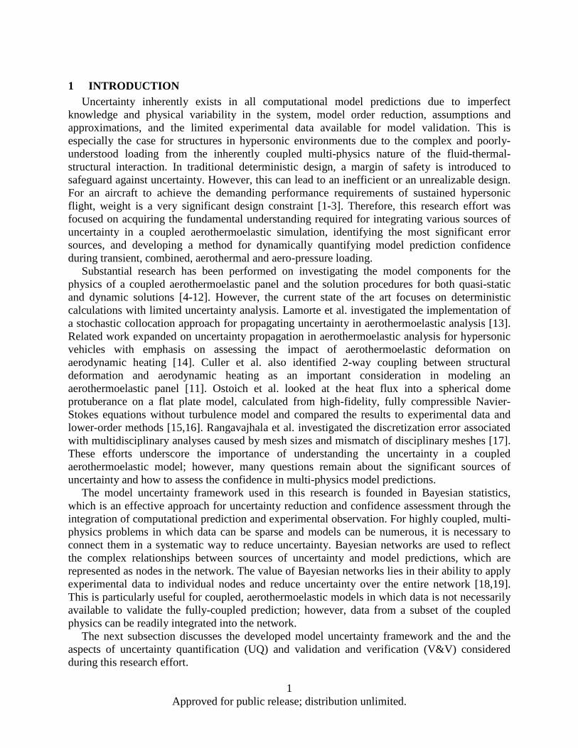
Considering the UQ and V&V discussion above, a framework for quantifying model prediction confidence for hypersonic aerostructures was developed and is shown in Figure 1.1. The first component focuses on characterizing model uncertainty, which is accomplished by constructing a Bayesian network and calibrating the uncertain parameters and model discrepancy [20-22]. This is not just about quantifying the uncertainty in each of the individual uni-disciplinary constituent models, but rather about quantifying the uncertainty in the coupled interactions of the multi-fidelity, multi-physics models, as well. The second component addresses efficiently propagating the model uncertainties forward to a quantity of interest (QoI) in the coupled system. In this construct, the sensitivity of the QoI to each of the uncertain inputs and model errors can be evaluated, which is important for identifying where to focus the resources for uncertainty reduction efforts. The third and final component is managing the uncertainty by using data for multiple different purposes, such as prediction confidence assessment, model validation, and/or model selection.
2 Approved for public release; distribution unlimited.
Figure 1.1. Framework for integrating of models, data, and uncertainty
1.2 Report Overview and Outline This Lab Task effort takes the initial steps in a longer-term research plan for developing a
framework for integrating various sources of uncertainty in a coupled hypersonic structural simulation and assessing the confidence in model predictions. The FY12-14 Lab Task consisted of three primary objectives. The first objective is to develop a systematic framework for enabling the integration of the various sources of uncertainty from the individual disciplines of a fully-coupled system. The second objective is to investigate uncertainty quantification and analysis of fluid-thermal-structural interactions in hypersonic flow. The third objective is to provide a decision-making metric for determining the necessary model fidelity and degree of coupling to achieve the desired level of confidence in the system prediction. All three objectives play a critical role in assessing the predictive capability of a coupled aerothermoelastic system model. The objectives were addressed through several related investigations, presented in Sections 3-8 of this final report.
Section 2 introduces the aerothermoelastic coupled system considered throughout this research, including aerothermal models and historic high-speed wind test data. The first year of this research (Section 3) focused on identifying and developing the components of the model uncertainty framework for aerodynamic pressure and heating predictions, including global sensitivity analysis, Bayesian model calibration, and confidence assessment [23,31]. The second year emphasized effectively integrating information into the coupled system through segmented Bayesian model calibration, as well as using time-dependent aerothermal data in the Bayesian network, discussed in Sections 4 and 5, respectively [24,25,33]. A pre-validation study was also conducted (Section 7) for the historic aerothermal data to determine if the models being considered adequately captured the observed flow characteristics [27]. The third year brought together model discrepancy in aerodynamic pressure calibrated from aerothermal experiments with nonlinear structural dynamic reduced order models to investigate the uncertainty and sensitivity in coupled aeroelastic response (i.e., flutter and limit cycle oscillation), which is covered in Section 6 [26,32,34]. Finally, many real world systems have discrete operating states,
3 Approved for public release; distribution unlimited.

e.g., pre-buckled or post-buckled columns, laminar or turbulent flow, elastic or plastic response, and various stages of wear. Identification of precise boundaries between states is typically very challenging due to incomplete understanding of physical processes and experimental uncertainty. In Section 8, a method was developed for quantifying the uncertainty in state boundaries for thin beam buckling [28,35,36].
4 Approved for public release; distribution unlimited.
2 AEROTHERMOELASTIC COUPLING Aircraft structures exposed to extreme environments are subjected to coupled aerodynamic,
thermal, and acoustic loading [4-12]. Neglecting these interactions can lead to gross errors in model predictions [10-13,38,39].To account for these uncertainties, hypersonic aircraft structures must be designed to within accurately-quantified safety margins that are not overly conservative, so that the platform can have the minimum structural weight that permits proper execution of the mission objectives [40]. When the structure is designed to these margins, it must necessarily operate at the intersection of the applicable technical disciplines associated with extreme hypersonic environments, and be able to withstand intense, coupled, structural, fluid, thermal, and acoustic loads [4-8].
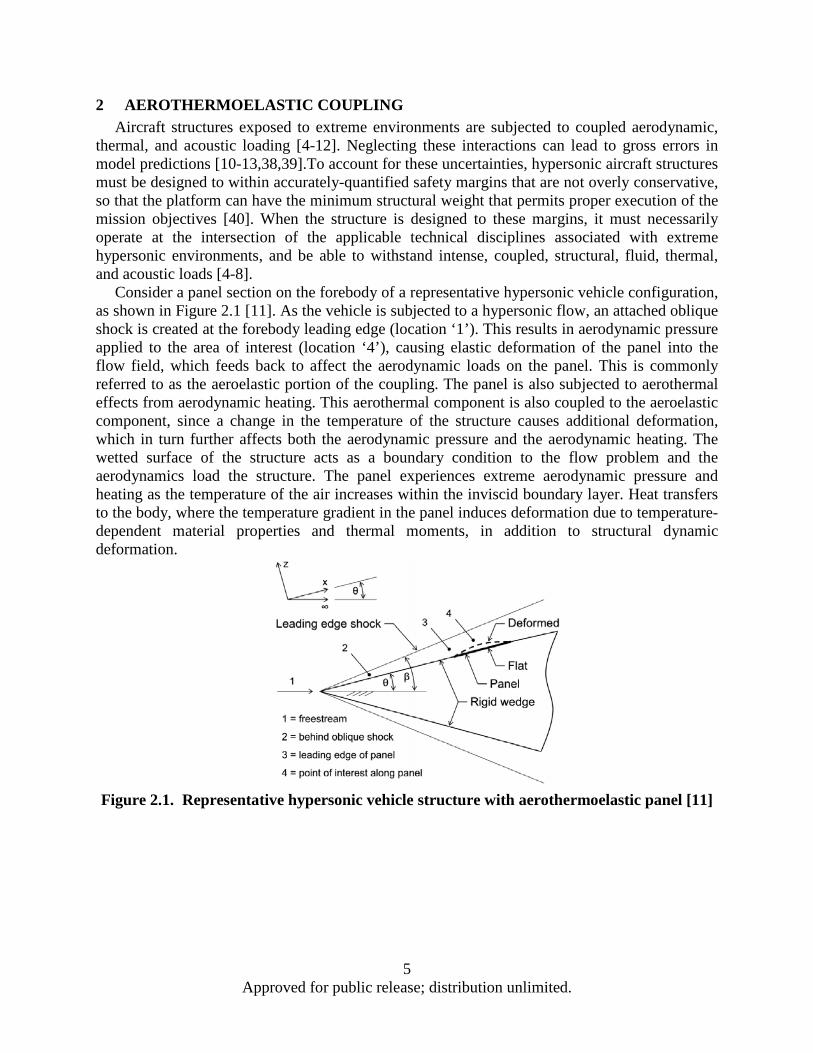
Consider a panel section on the forebody of a representative hypersonic vehicle configuration, as shown in Figure 2.1 [11]. As the vehicle is subjected to a hypersonic flow, an attached oblique shock is created at the forebody leading edge (location ‘1’). This results in aerodynamic pressure applied to the area of interest (location ‘4’), causing elastic deformation of the panel into the flow field, which feeds back to affect the aerodynamic loads on the panel. This is commonly referred to as the aeroelastic portion of the coupling. The panel is also subjected to aerothermal effects from aerodynamic heating. This aerothermal component is also coupled to the aeroelastic component, since a change in the temperature of the structure causes additional deformation, which in turn further affects both the aerodynamic pressure and the aerodynamic heating. The wetted surface of the structure acts as a boundary condition to the flow problem and the aerodynamics load the structure. The panel experiences extreme aerodynamic pressure and heating as the temperature of the air increases within the inviscid boundary layer. Heat transfers to the body, where the temperature gradient in the panel induces deformation due to temperature-dependent material properties and thermal moments, in addition to structural dynamic deformation.
Figure 2.1. Representative hypersonic vehicle structure with aerothermoelastic panel [11]
5 Approved for public release; distribution unlimited.
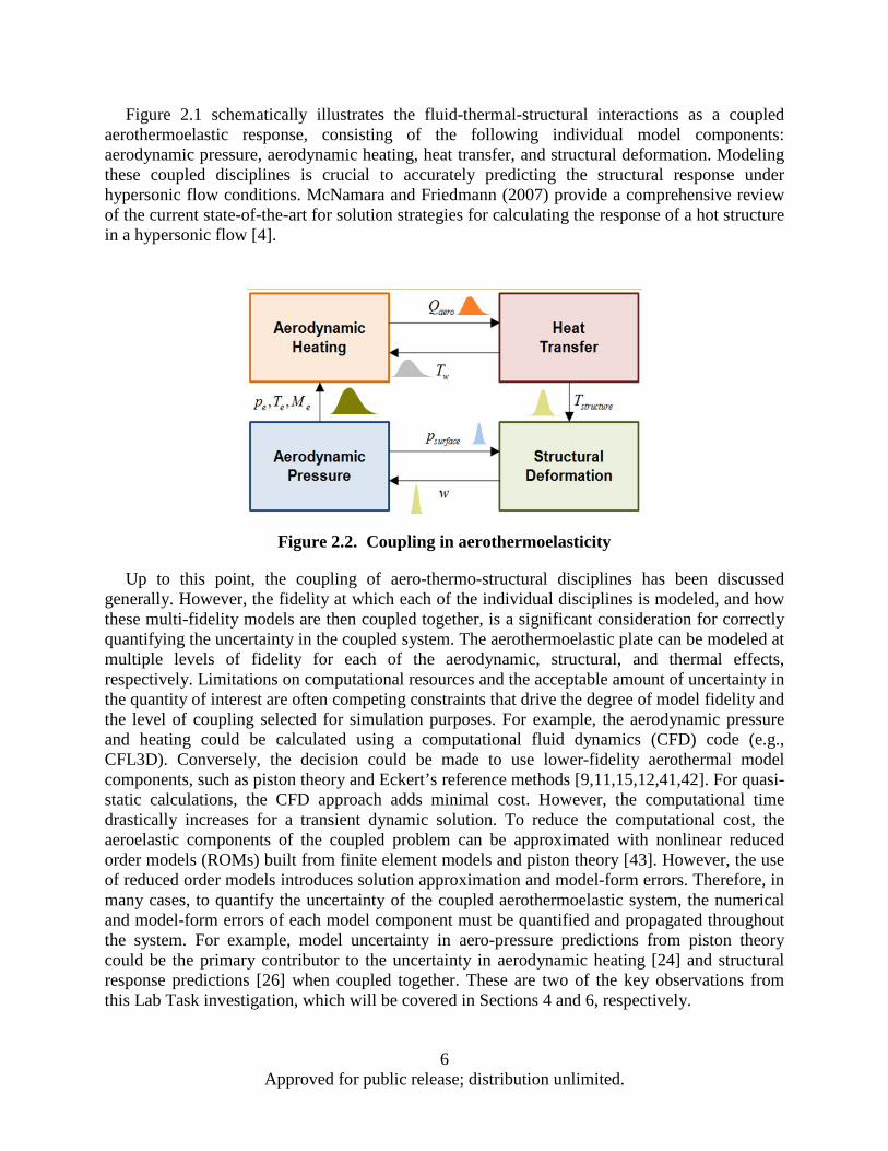
Figure 2.1 schematically illustrates the fluid-thermal-structural interactions as a coupled aerothermoelastic response, consisting of the following individual model components: aerodynamic pressure, aerodynamic heating, heat transfer, and structural deformation. Modeling these coupled disciplines is crucial to accurately predicting the structural response under hypersonic flow conditions. McNamara and Friedmann (2007) provide a comprehensive review of the current state-of-the-art for solution strategies for calculating the response of a hot structure in a hypersonic flow [4].
Figure 2.2. Coupling in aerothermoelasticity
Up to this point, the coupling of aero-thermo-structural disciplines has been discussed generally. However, the fidelity at which each of the individual disciplines is modeled, and how these multi-fidelity models are then coupled together, is a significant consideration for correctly quantifying the uncertainty in the coupled system. The aerothermoelastic plate can be modeled at multiple levels of fidelity for each of the aerodynamic, structural, and thermal effects, respectively. Limitations on computational resources and the acceptable amount of uncertainty in the quantity of interest are often competing constraints that drive the degree of model fidelity and the level of coupling selected for simulation purposes. For example, the aerodynamic pressure and heating could be calculated using a computational fluid dynamics (CFD) code (e.g., CFL3D). Conversely, the decision could be made to use lower-fidelity aerothermal model components, such as piston theory and Eckert’s reference methods [9,11,15,12,41,42]. For quasi-static calculations, the CFD approach adds minimal cost. However, the computational time drastically increases for a transient dynamic solution. To reduce the computational cost, the aeroelastic components of the coupled problem can be approximated with nonlinear reduced order models (ROMs) built from finite element models and piston theory [43]. However, the use of reduced order models introduces solution approximation and model-form errors. Therefore, in many cases, to quantify the uncertainty of the coupled aerothermoelastic system, the numerical and model-form errors of each model component must be quantified and propagated throughout the system. For example, model uncertainty in aero-pressure predictions from piston theory could be the primary contributor to the uncertainty in aerodynamic heating [24] and structural response predictions [26] when coupled together. These are two of the key observations from this Lab Task investigation, which will be covered in Sections 4 and 6, respectively.
6 Approved for public release; distribution unlimited.
The next section defines several of the model components in the aerothermoelastic system shown in Figure 2.2.
2.1 Aerothermoelastic Models Given the freestream flight conditions (p1, M1, T1) and the surface inclination angle (θ) from
Figure 2.1, the local conditions at the leading edge of the panel (p3, M3, T3) resulting from an oblique shockwave can be computed using oblique shock relations, shown in Eqs. (2.1) - (2.4). The oblique shock calculations do not have any dependency on the geometry of the panel itself, solely the surface inclination of the forebody and freestream conditions. Thus, it is only valid at locations where no structural deformation is present (i.e. flat plate).
2 231
1
21 ( sin 1)1
p Mp
γ βγ
= + −+
(2.1)
2 2
3 12 2
1 1
( 1) sin ( )( 1) sin ( ) 2
MM
ρ γ βρ γ β
+=
− + (2.2)
3 3 1
1 3 1
//
T p pT ρ ρ
= (2.3)
2 21
2 23
2 21
2sin ( )1sin ( ) 2( ) sin ( ) 1
1
MM
M
βγβ θβ
γ
+−− =
−−
(2.4)
Once the flow properties at the leading edge of the panel are calculated from oblique shock relations, piston theory provides a simplified relationship between the unsteady pressure on the panel and turbulent surface pressure [41]. This simple model is desired for computational tractability and uses the leading edge conditions to approximate the aerodynamic pressure load chord-wise across the panel (p4, M4, T4). In piston theory, the pressure prediction is dependent on the slope of the panel (∂w/∂x) and the velocity of deformation (∂w/∂t). A 3rd-order expansion of piston theory is presented in Eq. (2.5).
2 3
234 3 3 3
3 3 3 3
1 1 1 1 124 12
q w w w w w wp p M MM U t x U t x U t x
γ γ ∂ ∂ + ∂ ∂ + ∂ ∂ = + + + + + + ∂ ∂ ∂ ∂ ∂ ∂ (2.5)
After calculating the aerodynamic pressure and flow conditions along the panel surface, the aerodynamic heat flux is predicted using the computationally efficient Eckert's reference temperature method assuming a calorically perfect gas [42]. The Eckert's reference temperature is computed by Eq. (2.6) and the heat flux across the spherical dome follows in Eq. (2.7).
*3 30.5( ) 0.22( )w e awT T T T T T= + − + − (2.6)
7 Approved for public release; distribution unlimited.
* * *4 ( )e p aw wQ St U c T Tρ= − (2.7)
where, St* is the reference Stanton number, ρ* is the reference density, Ue is the inviscid flow velocity at the dome location, *
pc is the reference specific heat, Taw and Tw are the adiabatic wall and actual wall temperature, respectively and Te is the boundary layer edge temperature.
2.2 Aerothermal Experiments Accurately modeling aero-thermo-elastic response for hypersonic aircraft structures is
obviously challenging, especially due to the inability to replicate the bulk of the in-flight loading conditions through ground test facilities and hence improve the models being used. Laboratory experiments to approximate these unfamiliar flight environments is the other half of ensuring accurate aero-thermo-acoustic modeling. However, the available experimental techniques and facilities are not fully capable of simultaneously capturing coupled aerothermoelastic response in hypersonic flow. Therefore, we must rely on maximizing the utility of whatever data can be acquired, or may already be available, for a subset of the multi-physics interactions. For example, historical tests performed by Glass and Hunt in 1986 at NASA’s 8ft High-Temperature Wind Tunnel (HTT) investigated the thermal and structural loads on body panels in hypersonic environments [44]. These tests measured the aerodynamic pressure and heating on spherical dome protuberances into the flow that simulated deformed aircraft panels. But these tests were performed on rigid domes protruding into the flow and were not instrumented to measure structural response, thus the dynamic structural response was not captured. The 8-foot High-Temperature Tunnel can simulate up to Mach 7 flow at an altitude between 25 and 40 km for up to 2 minutes by combusting a mixture of methane and air. The flow conditions for the tests of interest had a turbulent boundary-layer at the panel location, and the panel holder had a sharp leading edge, similar to the representative hypersonic vehicle depicted in Figure 2.1.
The experiments performed by Glass and Hunt used a flat plate specimen to record the aerodynamic pressure and heat flux at the center of the plate as a reference. In addition, spherical pressure and thermal domes with a diameter of 35.6 cm and the three H/D ratios shown in Table 2.1 were instrumented. Table 2.1 also summarizes the freestream conditions p1 and M1, for each test. A schematic of the test specimen and the 58 instrumented locations is shown in Figure 2.3. For the purposes of this study, the analysis is limited to the points along the centerline parallel to the flow. An investigation by Ostoich et al. [15,16] discovered that the recorded data at points 1 and 38 may have been affected by an uncharacterized gap between the dome and plate, thus only the middle 11 data points along the centerline (points 2-39) were considered.
8 Approved for public release; distribution unlimited.
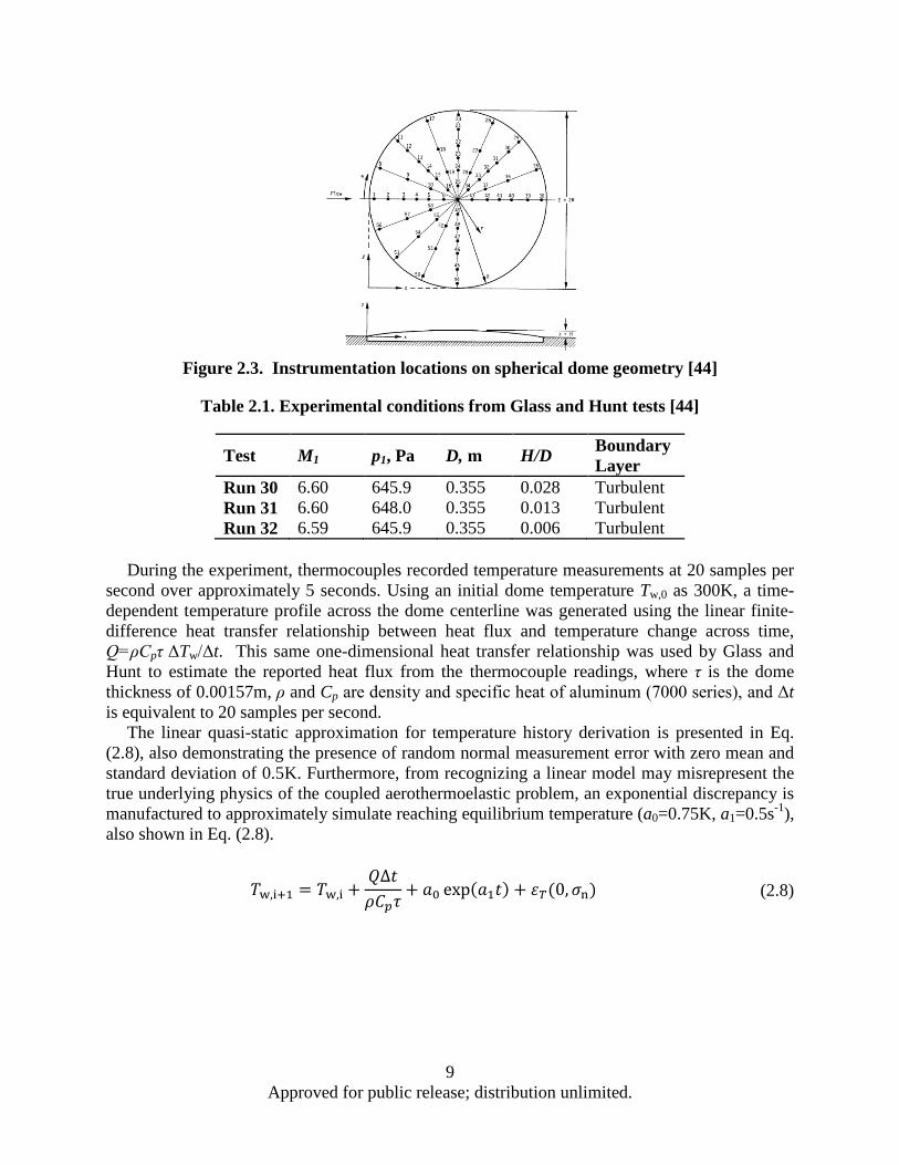
Figure 2.3. Instrumentation locations on spherical dome geometry [44]
Table 2.1. Experimental conditions from Glass and Hunt tests [44]
During the experiment, thermocouples recorded temperature measurements at 20 samples per
second over approximately 5 seconds. Using an initial dome temperature Tw,0 as 300K, a time-dependent temperature profile across the dome centerline was generated using the linear finite-difference heat transfer relationship between heat flux and temperature change across time, Q=ρCpτ ΔTw/Δt. This same one-dimensional heat transfer relationship was used by Glass and Hunt to estimate the reported heat flux from the thermocouple readings, where τ is the dome thickness of 0.00157m, ρ and Cp are density and specific heat of aluminum (7000 series), and Δt is equivalent to 20 samples per second.
The linear quasi-static approximation for temperature history derivation is presented in Eq. (2.8), also demonstrating the presence of random normal measurement error with zero mean and standard deviation of 0.5K. Furthermore, from recognizing a linear model may misrepresent the true underlying physics of the coupled aerothermoelastic problem, an exponential discrepancy is manufactured to approximately simulate reaching equilibrium temperature (a0=0.75K, a1=0.5s-1), also shown in Eq. (2.8).
𝑇𝑇w,i+1 = 𝑇𝑇w,i +𝑄𝑄Δ𝑡𝑡𝜌𝜌𝐶𝐶𝑝𝑝𝜏𝜏
+ 𝑎𝑎0 exp(𝑎𝑎1𝑡𝑡) + 𝜀𝜀𝑇𝑇(0,𝜎𝜎n) (2.8)
Test M1 p1, Pa D, m H/D Boundary Layer
Run 30 6.60 645.9 0.355 0.028 Turbulent Run 31 6.60 648.0 0.355 0.013 Turbulent Run 32 6.59 645.9 0.355 0.006 Turbulent
9 Approved for public release; distribution unlimited.

Figure 2.4. Estimated transient temperature distributions from Runs 30, 31, and 32
The temperature profiles over 5 seconds in Runs 30, 31, and 32 are shown in Figure 2.4. There is an absence of two Run 31 transient temperature histories along the dome due to missing heat flux measurements those points. The transient aerothermal data is used in this investigation for Bayesian model calibration and prediction confidence assessment for coupled, time-dependent aerothermal analysis.
10 Approved for public release; distribution unlimited.
3 ERROR QUANTIFICATION AND CONFIDENCE ASSESSMENT OF AEROTHERMAL MODEL PREDICTIONS
This section analyzes the prediction error for the Glass and Hunt experiments [44] using the assumptions and results from Culler et al. [11]. This work reevaluates some of the assumptions and errors that were observed in the previous study.
First, a description of the uncertain input parameters in the experiments and aerodynamic pressure and heating calculations is provided with sensitivity analysis. Next, two sets of experimental data are used to calibrate uncertain model inputs and errors. The calibrated inputs are then used to update nominal predictions for the spherical dome experiments. Then, a third data set is used for validation with Bayesian hypothesis testing-based confidence. Finally, a model selection study is performed using the confidence metric for different forms of piston theory.
3.1 Model Input Uncertainty and Sensitivity Analysis Consider the flat plate specimen, where oblique shock relations are used for aerodynamic
pressure 4fpp and Eckert’s reference temperature method for aerodynamic heating 4
fpQ . Note that for the flat plate, we are interested in the value at the center of the plate, which corresponds to location ‘4’ in Figure 2.1. The flat plate experiments consisted of three tests (Runs 30, 31, and 32), which all correspond to the same nominal inputs and turbulent boundary-layer with a sharp leading edge panel holder. For these tests, the freestream pressure p1, and Mach number M1, were given as shown in Table 2.1. In addition, the output aerodynamic pressure and heat flux were measured at the center of the flat plate. However, three critical pieces of information were not available in the Glass and Hunt report [44]: the freestream temperature T1, wall temperature Tw4, and equivalence ratio Req. Therefore, realistic values had to be estimated from other reports of similar testing.24 The mean freestream and wall temperatures are assumed to be 220K and 300K, respectively. The equivalence ratio is also uncertain, but for the current investigation a constant value of Req = 0.9 is assumed.
To get a better understanding of the uncertainty in the outputs and their sensitivity to the inputs, statistical distributions were assumed for the inputs. Since p1 and M1 were measured, 1% coefficient of variation (CV) is used for measurement variability. However, 10% CV is used for T1 and Tw4 since they were not reported and had to be assumed. Normal distributions are used for all four random inputs and their distribution parameters are shown in Table 3.1.
Table 3.1. Uncertainty for inputs to aerodynamic pressure and heat flux calculations Measured
Inputs Mean Standard Deviation
Coefficient of Variation
p1 (Pa) 652.5 6.525 1% M1 6.6 0.066 1%
Uncertain Inputs Mean Standard
Deviation Coefficient of
Variation T1 (K) 220 22.0 10% Tw4 (K) 300 30.0 10%
11 Approved for public release; distribution unlimited.
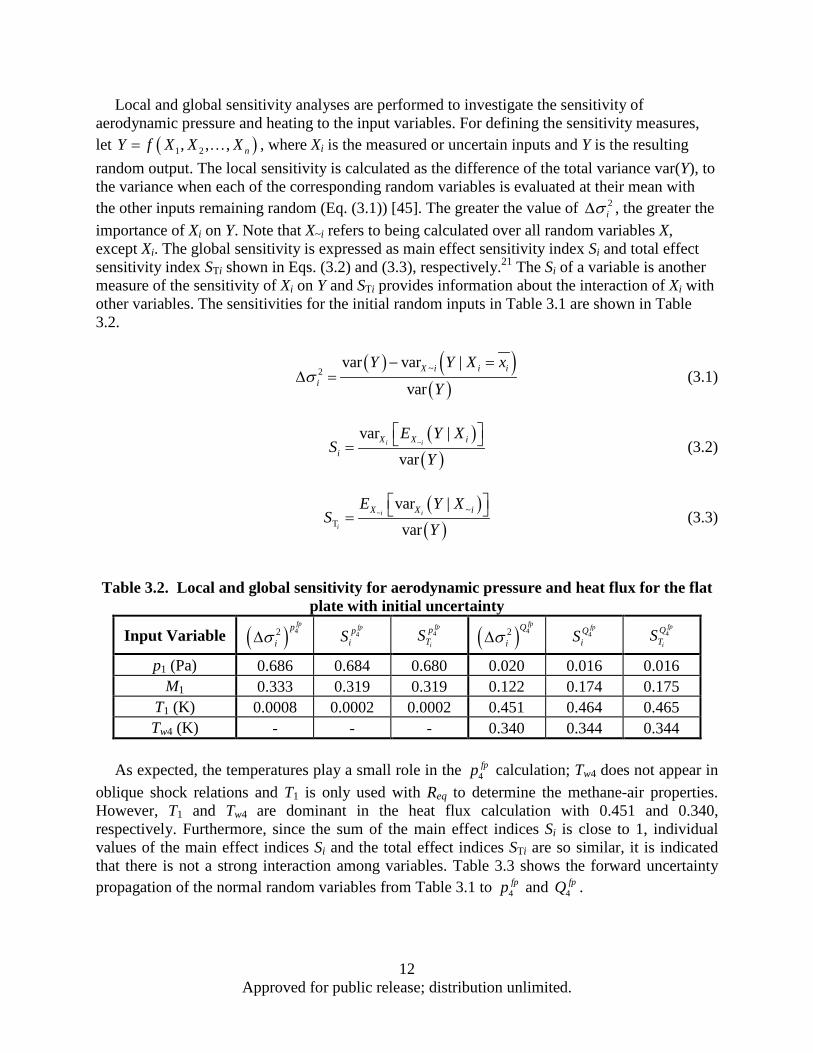
Local and global sensitivity analyses are performed to investigate the sensitivity of aerodynamic pressure and heating to the input variables. For defining the sensitivity measures, let ( )1 2, , , nY f X X X= 2 , where Xi is the measured or uncertain inputs and Y is the resulting random output. The local sensitivity is calculated as the difference of the total variance var(Y), to the variance when each of the corresponding random variables is evaluated at their mean with the other inputs remaining random (Eq. (3.1)) [45]. The greater the value of 2
iσ∆ , the greater the importance of Xi on Y. Note that X~i refers to being calculated over all random variables X, except Xi. The global sensitivity is expressed as main effect sensitivity index Si and total effect sensitivity index STi shown in Eqs. (3.2) and (3.3), respectively.21 The Si of a variable is another measure of the sensitivity of Xi on Y and STi provides information about the interaction of Xi with other variables. The sensitivities for the initial random inputs in Table 3.1 are shown in Table 3.2.
( ) ( )
( )~2
var var |
varX i i i
i
Y Y X x
Yσ
− =∆ = (3.1)
( )
( )~
var |
vari iX X i
i
E Y XS
Y
= (3.2)
( )( )
~ ~T
var |
vari i
i
X X iE Y XS
Y
= (3.3)
Table 3.2. Local and global sensitivity for aerodynamic pressure and heat flux for the flat
plate with initial uncertainty
Input Variable ( ) 42fpp
iσ∆ 4fpp
iS 4fp
i
pTS ( ) 42
fpQ
iσ∆ 4fpQ
iS
4fp
i
QTS
p1 (Pa) 0.686 0.684 0.680 0.020 0.016 0.016
M1 0.333 0.319 0.319 0.122 0.174 0.175 T1 (K) 0.0008 0.0002 0.0002 0.451 0.464 0.465 Tw4 (K) - - - 0.340 0.344 0.344
As expected, the temperatures play a small role in the 4
fpp calculation; Tw4 does not appear in oblique shock relations and T1 is only used with Req to determine the methane-air properties. However, T1 and Tw4 are dominant in the heat flux calculation with 0.451 and 0.340, respectively. Furthermore, since the sum of the main effect indices Si is close to 1, individual values of the main effect indices Si and the total effect indices STi are so similar, it is indicated that there is not a strong interaction among variables. Table 3.3 shows the forward uncertainty propagation of the normal random variables from Table 3.1 to 4
fpp and 4fpQ .
12 Approved for public release; distribution unlimited.
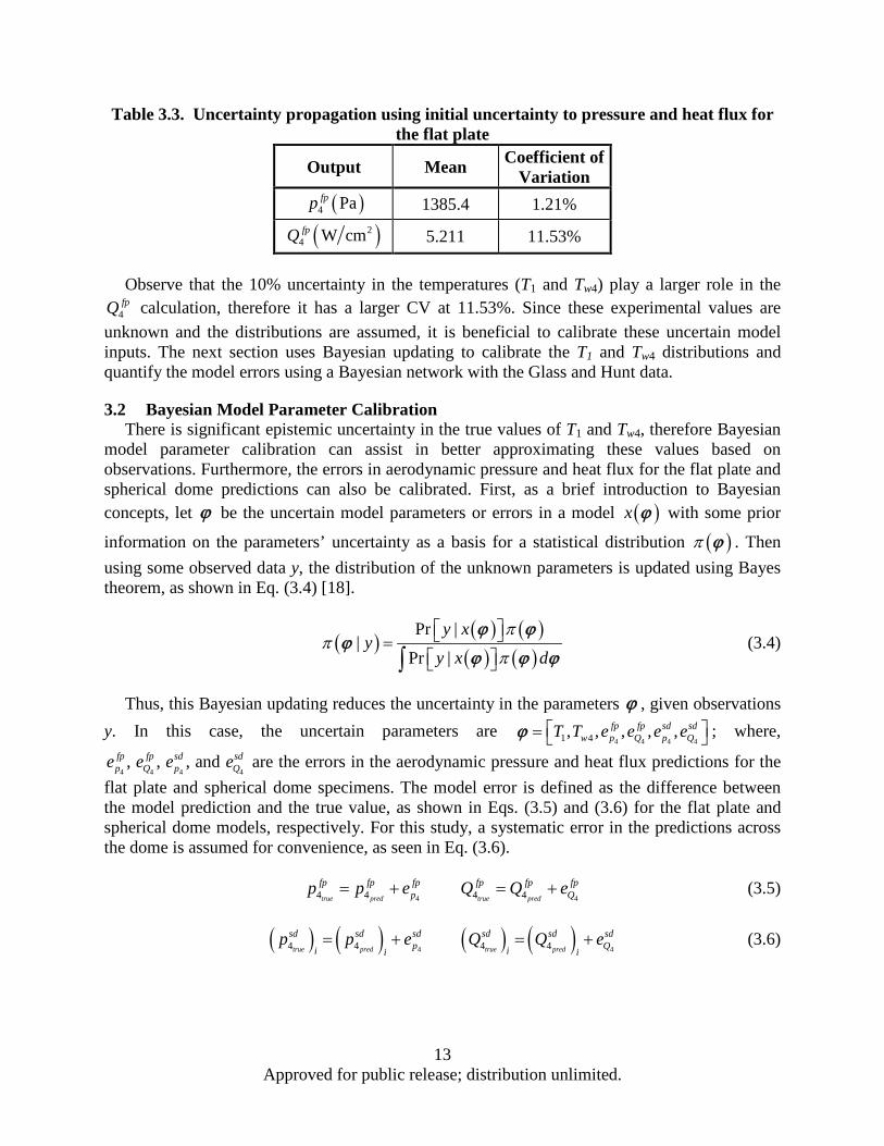
Table 3.3. Uncertainty propagation using initial uncertainty to pressure and heat flux for the flat plate
Output Mean Coefficient of Variation
( )4 Pafpp 1385.4 1.21%
( )24 W cmfpQ 5.211 11.53%
Observe that the 10% uncertainty in the temperatures (T1 and Tw4) play a larger role in the
4fpQ calculation, therefore it has a larger CV at 11.53%. Since these experimental values are
unknown and the distributions are assumed, it is beneficial to calibrate these uncertain model inputs. The next section uses Bayesian updating to calibrate the T1 and Tw4 distributions and quantify the model errors using a Bayesian network with the Glass and Hunt data.
3.2 Bayesian Model Parameter Calibration There is significant epistemic uncertainty in the true values of T1 and Tw4, therefore Bayesian
model parameter calibration can assist in better approximating these values based on observations. Furthermore, the errors in aerodynamic pressure and heat flux for the flat plate and spherical dome predictions can also be calibrated. First, as a brief introduction to Bayesian concepts, let ϕ be the uncertain model parameters or errors in a model ( )x ϕ with some prior
information on the parameters’ uncertainty as a basis for a statistical distribution ( )π ϕ . Then using some observed data y, the distribution of the unknown parameters is updated using Bayes theorem, as shown in Eq. (3.4) [18].
( ) ( ) ( )( ) ( )
Pr ||
Pr |
y xy
y x d
ππ
π
= ∫
ϕ ϕϕ
ϕ ϕ ϕ (3.4)
Thus, this Bayesian updating reduces the uncertainty in the parameters ϕ , given observations y. In this case, the uncertain parameters are
4 4 4 41 4, , , , ,fp fp sd sdw p Q p QT T e e e e = ϕ ; where,
4 4 4 4, , , andfp fp sd sd
p Q p Qe e e e are the errors in the aerodynamic pressure and heat flux predictions for the flat plate and spherical dome specimens. The model error is defined as the difference between the model prediction and the true value, as shown in Eqs. (3.5) and (3.6) for the flat plate and spherical dome models, respectively. For this study, a systematic error in the predictions across the dome is assumed for convenience, as seen in Eq. (3.6).
44 4true pred
fp fp fppp p e= +
44 4true pred
fp fp fpQQ Q e= + (3.5)
( ) ( ) 44 4true pred
sd sd sdpi i
p p e= + ( ) ( ) 44 4true pred
sd sd sdQi i
Q Q e= + (3.6)
13 Approved for public release; distribution unlimited.
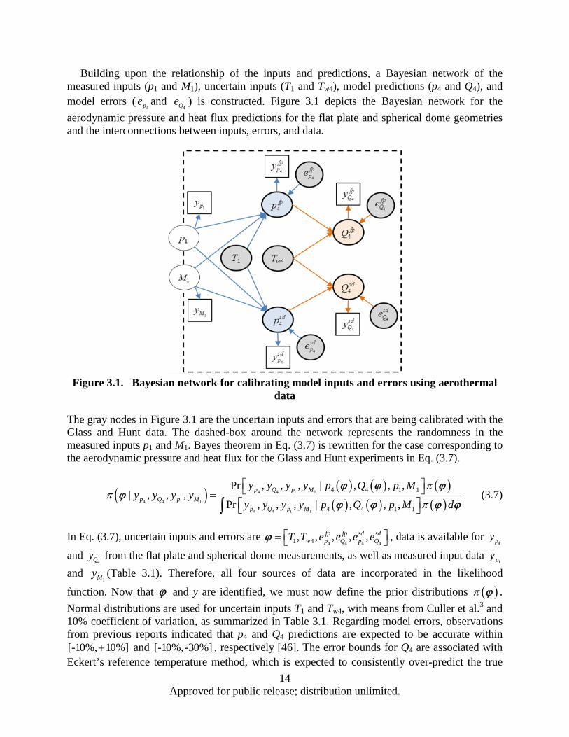
Building upon the relationship of the inputs and predictions, a Bayesian network of the measured inputs (p1 and M1), uncertain inputs (T1 and Tw4), model predictions (p4 and Q4), and model errors (
4pe and 4Qe ) is constructed. Figure 3.1 depicts the Bayesian network for the
aerodynamic pressure and heat flux predictions for the flat plate and spherical dome geometries and the interconnections between inputs, errors, and data.
Figure 3.1. Bayesian network for calibrating model inputs and errors using aerothermal
data
The gray nodes in Figure 3.1 are the uncertain inputs and errors that are being calibrated with the Glass and Hunt data. The dashed-box around the network represents the randomness in the measured inputs p1 and M1. Bayes theorem in Eq. (3.7) is rewritten for the case corresponding to the aerodynamic pressure and heat flux for the Glass and Hunt experiments in Eq. (3.7).
( ) ( ) ( ) ( )( ) ( ) ( )
4 4 1 1
4 4 1 1
4 4 1 1
4 4 1 1
4 4 1 1
Pr , , , | , , ,| , , ,
Pr , , , | , , ,p Q p M
p Q p Mp Q p M
y y y y p Q p My y y y
y y y y p Q p M d
ππ
π
= ∫
ϕ ϕ ϕϕ
ϕ ϕ ϕ ϕ (3.7)
In Eq. (3.7), uncertain inputs and errors are 4 4 4 41 4, , , , ,fp fp sd sd
w p Q p QT T e e e e = ϕ , data is available for 4py
and 4Qy from the flat plate and spherical dome measurements, as well as measured input data
1py and
1My (Table 3.1). Therefore, all four sources of data are incorporated in the likelihood
function. Now that ϕ and y are identified, we must now define the prior distributions ( )π ϕ . Normal distributions are used for uncertain inputs T1 and Tw4, with means from Culler et al.3 and 10% coefficient of variation, as summarized in Table 3.1. Regarding model errors, observations from previous reports indicated that p4 and Q4 predictions are expected to be accurate within [-10%, 10%]+ and [-10%,-30%] , respectively [46]. The error bounds for Q4 are associated with Eckert’s reference temperature method, which is expected to consistently over-predict the true
14 Approved for public release; distribution unlimited.
value due to the calorically perfect gas assumption. However, after a preliminary comparison of predictions to data, a uniform distribution over the range [-30%, +30%] of the prediction was determined to be a more appropriate prior for all four error terms in this study. Therefore, this error model assumes uniform distributions based on the experimental means for the prior distribution of errors ( )π ϕ . Normal distributions are used for the likelihood function
( )Pr |y x ϕ , where the distribution parameters from Table 3.2 are assumed for 1py and
1My , whereas 5% measurement uncertainty is assumed for aerodynamic pressure and heat flux measurements
4py and 4Qy .
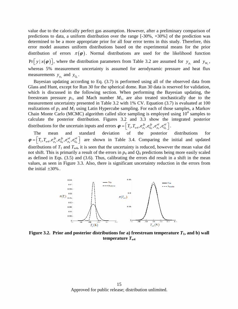
Bayesian updating according to Eq. (3.7) is performed using all of the observed data from Glass and Hunt, except for Run 30 for the spherical dome. Run 30 data is reserved for validation, which is discussed in the following section. When performing the Bayesian updating, the freestream pressure p1, and Mach number M1, are also treated stochastically due to the measurement uncertainty presented in Table 3.2 with 1% CV. Equation (3.7) is evaluated at 100 realizations of p1 and M1 using Latin Hypercube sampling. For each of those samples, a Markov Chain Monte Carlo (MCMC) algorithm called slice sampling is employed using 104 samples to calculate the posterior distribution. Figures 3.2 and 3.3 show the integrated posterior distributions for the uncertain inputs and errors
4 4 4 41 4, , , , ,fp fp sd sdw p Q p QT T e e e e = ϕ .
The mean and standard deviation of the posterior distributions for
4 4 4 41 4, , , , ,fp fp sd sdw p Q p QT T e e e e = ϕ are shown in Table 3.4. Comparing the initial and updated
distributions of T1 and Tw4, it is seen that the uncertainty is reduced, however the mean value did not shift. This is primarily a result of the errors in p4 and Q4 predictions being more easily scaled as defined in Eqs. (3.5) and (3.6). Thus, calibrating the errors did result in a shift in the mean values, as seen in Figure 3.3. Also, there is significant uncertainty reduction in the errors from the initial 30%± .
Figure 3.2. Prior and posterior distributions for a) freestream temperature T1, and b) wall
temperature Tw4
15 Approved for public release; distribution unlimited.
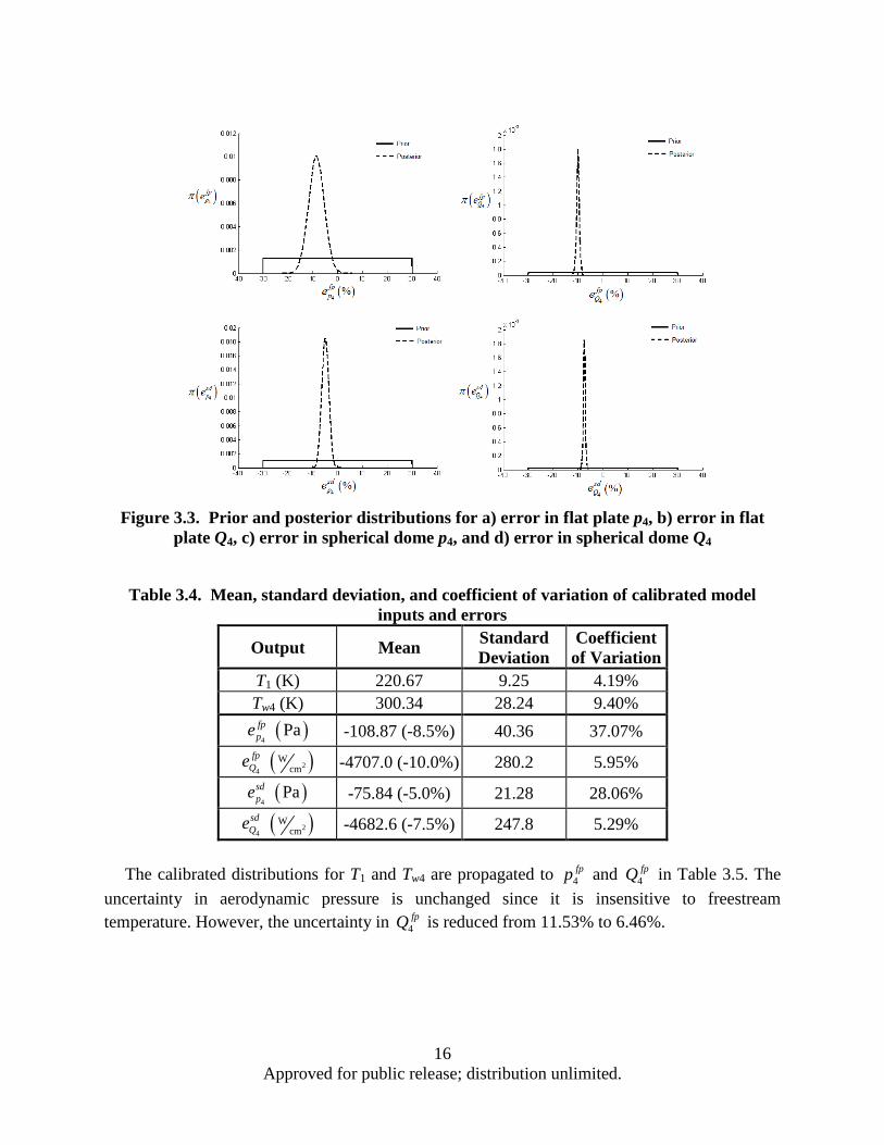
Figure 3.3. Prior and posterior distributions for a) error in flat plate p4, b) error in flat
plate Q4, c) error in spherical dome p4, and d) error in spherical dome Q4
Table 3.4. Mean, standard deviation, and coefficient of variation of calibrated model
inputs and errors
Output Mean Standard Deviation
Coefficient of Variation
T1 (K) 220.67 9.25 4.19% Tw4 (K) 300.34 28.24 9.40%
( )4
Pafppe -108.87 (-8.5%) 40.36 37.07%
( )24
Wcm
fpQe -4707.0 (-10.0%) 280.2 5.95%
( )4
Pasdpe -75.84 (-5.0%) 21.28 28.06%
( )24
Wcm
sdQe -4682.6 (-7.5%) 247.8 5.29%
The calibrated distributions for T1 and Tw4 are propagated to 4
fpp and 4fpQ in Table 3.5. The
uncertainty in aerodynamic pressure is unchanged since it is insensitive to freestream temperature. However, the uncertainty in 4
fpQ is reduced from 11.53% to 6.46%.
16 Approved for public release; distribution unlimited.
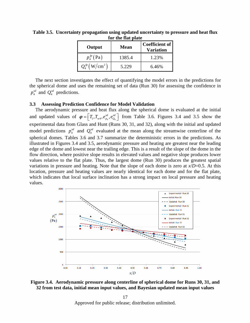
Table 3.5. Uncertainty propagation using updated uncertainty to pressure and heat flux for the flat plate
Output Mean Coefficient of Variation
( )4 Pafpp 1385.4 1.23%
( )24 W cmfpQ 5.229 6.46%
The next section investigates the effect of quantifying the model errors in the predictions for
the spherical dome and uses the remaining set of data (Run 30) for assessing the confidence in 4sdp and 4
sdQ predictions.
3.3 Assessing Prediction Confidence for Model Validation The aerodynamic pressure and heat flux along the spherical dome is evaluated at the initial
and updated values of 4 41 4, , ,sd sd
w p QT T e e = ϕ from Table 3.6. Figures 3.4 and 3.5 show the experimental data from Glass and Hunt (Runs 30, 31, and 32), along with the initial and updated model predictions 4
sdp and 4sdQ evaluated at the mean along the streamwise centerline of the
spherical domes. Tables 3.6 and 3.7 summarize the deterministic errors in the predictions. As illustrated in Figures 3.4 and 3.5, aerodynamic pressure and heating are greatest near the leading edge of the dome and lowest near the trailing edge. This is a result of the slope of the dome in the flow direction, where positive slope results in elevated values and negative slope produces lower values relative to the flat plate. Thus, the largest dome (Run 30) produces the greatest spatial variations in pressure and heating. Note that the slope of each dome is zero at x/D=0.5. At this location, pressure and heating values are nearly identical for each dome and for the flat plate, which indicates that local surface inclination has a strong impact on local pressure and heating values.
Figure 3.4. Aerodynamic pressure along centerline of spherical dome for Runs 30, 31, and
32 from test data, initial mean input values, and Bayesian updated mean input values
17 Approved for public release; distribution unlimited.

Table 3.6. Error summary for nominal pressure predictions along centerline of spherical dome
Initial Errors in 4sdp Updated Errors in 4
sdp Run 30 Run 31 Run 32 Run 30 Run 31 Run 32
Average 13.6% 8.2% 6.7% 16.0% 8.3% 2.7% Maximum 39.3% 23.5% 14.2% 35.4% 18.5% 8.9%
From Figure 3.4 and Table 3.6 it is evident that 3rd-order piston theory predictions of 4
sdpbecome less accurate with increasing dome surface inclination. Accordingly, the largest error in
4sdp occurs at the forward-most location in Run 30. Recall that Run 30 was saved for validation
and only Runs 31 and 32 were included in calibration. This generally resulted in smaller errors for Runs 31 and 32, but errors for Run 30 increased, as summarized in Table 3.6. It is expected that if data from Run 30 had been included in calibration, then the corresponding errors would have also been reduced. Furthermore, since the errors in 4
sdp along the dome vary in magnitude spatially, it would be beneficial to use a more flexible error model, such as a Gaussian process model, in more practical applications.
Figure 3.5 and Table 3.7 show that Eckert’s reference temperature method predicted 4sdQ
more accurately than 3rd-order piston theory predicted 4sdp . Again, the trend is observed that
errors are reduced using the updated ϕ values for Runs 31 and 32, but not Run 30. This may be expected since values of
4
sdQy from Runs 31 and 32 are included in the Bayesian calibration,
whereas values from Run 30 were not used.
Figure 3.5. Aerodynamic heat flux along centerline of spherical dome for Runs 30, 31, and
32 from experimental data, initial mean input values, and Bayesian updated mean input values
18 Approved for public release; distribution unlimited.

Table 3.7. Errors for nominal heat flux predictions along centerline of spherical dome Initial Errors - 4
sdQ Updated Errors - 4sdQ
Run 30 Run 31 Run 32 Run 30 Run 31 Run 32 Average 3.9% 6.2% 12.8% 11.7% 4.1% 3.6%
Maximum 12.9% 10.4% 21.2% 24.7% 8.7% 12.4% The deterministic errors are useful for assessing the accuracy of the nominal model
predictions, however this is a stochastic problem and error alone does not provide a statistical assessment of the confidence in the model prediction. Therefore, the most important step in this model uncertainty framework is to validate the models by assessing the confidence. This enables decision-making in regard to model development and fidelity selection. For the Aircraft Digital Twin, it is important to have this confidence metric to make autonomous decision making possible for efficient simulations and risk mitigation.
Several validation metrics exist with advantages and disadvantages, such as classical hypothesis testing, and difference and area metrics; however Bayesian hypothesis testing is selected for this study [47,48]. The Bayes factor approach fits appropriately with the Bayesian network integration framework, but its main advantages are that it takes into account the entire probability distribution of the model output and its relation to a confidence metric is straightforward. For Bayesian hypothesis testing, we want to determine the probability of our model being correct, given some observed data. Consider a hypothesis test to determine the probability that a model prediction x is equal to its true value x0. Equation (3.8) calculates the Bayes factor B, as the ratio of likelihoods corresponding to the null hypothesis (model prediction is equal to the true value) and the alternate hypothesis (model prediction is not equal to the true value). Therefore, when B > 1, the data supports the null hypothesis better than the alternative hypothesis. The integral form of the Bayes factor in Eq. (3.8) includes the likelihood function of the data supporting the prediction Pr(y|x), the probability density function (PDF) of the model prediction ( )0 xπ , and the PDF for the alternative hypothesis ( )1 xπ .
( ) ( )( )
( ) ( )( ) ( )
00 00
1 0 1
Pr |Pr | :Pr | : Pr |
y x x dxy H x xB x
y H x x y x x dx
π
π=
= =≠
∫∫
(3.8)
Equation (3.8) is rewritten in Eqs. (3.9) and (3.10) for the cases for aerodynamic pressure and heat flux, where i = 1 to 11 for the x-location across the dome.
( ) ( ) ( )( ) ( )
4
0
4
4 0 4 4
4
4 1 4 4
Pr |
Pr |
sd i i ii
i
sd i i ii
sd sd sdpsd
sd sd sdp
y p p dpB p
y p p dp
π
π=
∫∫
(3.9)
( ) ( ) ( )( ) ( )
4
0
4
4 0 4 4
4
4 1 4 4
Pr |
Pr |
sd i i ii
i
sd i i ii
sd sd sdQsd
sd sd sdQ
y Q Q dQB Q
y Q Q dQ
π
π=
∫∫
(3.10)
19 Approved for public release; distribution unlimited.
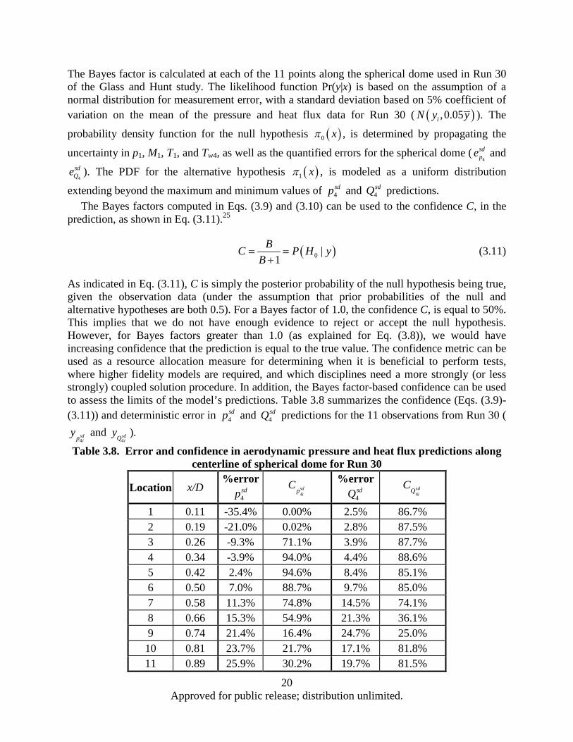
The Bayes factor is calculated at each of the 11 points along the spherical dome used in Run 30 of the Glass and Hunt study. The likelihood function Pr(y|x) is based on the assumption of a normal distribution for measurement error, with a standard deviation based on 5% coefficient of variation on the mean of the pressure and heat flux data for Run 30 ( ( ),0.05iN y y ). The
probability density function for the null hypothesis ( )0 xπ , is determined by propagating the
uncertainty in p1, M1, T1, and Tw4, as well as the quantified errors for the spherical dome (4
sdpe and
4
sdQe ). The PDF for the alternative hypothesis ( )1 xπ , is modeled as a uniform distribution
extending beyond the maximum and minimum values of 4sdp and 4
sdQ predictions. The Bayes factors computed in Eqs. (3.9) and (3.10) can be used to the confidence C, in the
prediction, as shown in Eq. (3.11).25
( )0 |1
BC P H yB
= =+
(3.11)
As indicated in Eq. (3.11), C is simply the posterior probability of the null hypothesis being true, given the observation data (under the assumption that prior probabilities of the null and alternative hypotheses are both 0.5). For a Bayes factor of 1.0, the confidence C, is equal to 50%. This implies that we do not have enough evidence to reject or accept the null hypothesis. However, for Bayes factors greater than 1.0 (as explained for Eq. (3.8)), we would have increasing confidence that the prediction is equal to the true value. The confidence metric can be used as a resource allocation measure for determining when it is beneficial to perform tests, where higher fidelity models are required, and which disciplines need a more strongly (or less strongly) coupled solution procedure. In addition, the Bayes factor-based confidence can be used to assess the limits of the model’s predictions. Table 3.8 summarizes the confidence (Eqs. (3.9)-(3.11)) and deterministic error in 4
sdp and 4sdQ predictions for the 11 observations from Run 30 (
4sd
ipy and
4sdiQ
y ).
Table 3.8. Error and confidence in aerodynamic pressure and heat flux predictions along centerline of spherical dome for Run 30
Location x/D %error
4sdp 4
sdip
C %error 4sdQ 4
sdiQ
C
1 0.11 -35.4% 0.00% 2.5% 86.7% 2 0.19 -21.0% 0.02% 2.8% 87.5% 3 0.26 -9.3% 71.1% 3.9% 87.7% 4 0.34 -3.9% 94.0% 4.4% 88.6% 5 0.42 2.4% 94.6% 8.4% 85.1% 6 0.50 7.0% 88.7% 9.7% 85.0% 7 0.58 11.3% 74.8% 14.5% 74.1% 8 0.66 15.3% 54.9% 21.3% 36.1% 9 0.74 21.4% 16.4% 24.7% 25.0% 10 0.81 23.7% 21.7% 17.1% 81.8% 11 0.89 25.9% 30.2% 19.7% 81.5%
20 Approved for public release; distribution unlimited.

The majority of the predictions have greater than 50% confidence, which means the data supports the prediction. Pressure predictions at locations 4-6 have the highest confidence. The confidence in 4
sdQ predictions using Eckert’s reference temperature method are all above 80%, with the exception of locations 7-9. As mentioned for Figure 3.4, the largest error in the 4
sdp occurs at the front of the dome, which corresponds to 0% confidence. The deterministic errors give an indication of the quality of the nominal predictions, however note that it is not always indicative of the statistical confidence in the predicted values. For example, 2.4% error at location 5 for 4
sdp corresponds to 94.6% confidence, but 2.5% error at location 1 for 4sdQ is
lower at 86.7% confidence. This is the result of differences in the shape of the model error distributions for 4
sdp and 4sdQ .
The scope of this work is to initiate a framework for assessing the confidence in coupled aerothermoelastic model predictions, not to necessarily draw definitive conclusions for these particular aerodynamic models. However, given the confidence associated with the 4
sdp predictions for Run 30 (H/D = 0.028), one would likely conclude that 3rd-order piston theory is inadequate for predicting the aerodynamic pressure on a spherical dome protuberance of this size. Although, to truly reach that conclusion, more thorough uncertainty quantification is required to better capture the model error.
The final section builds upon the conclusions using the Bayes factor-based confidence and uses that metric to compare predictions using different forms of piston theory.
3.4 Model Selection from Prediction Confidence Metric The Bayes factor-based confidence metric is also useful for model selection. Up to this point,
a 3rd-order expansion of piston theory from Eq. (2.5) was used to predict 4sdp . Naturally, 1st- and
2nd-order expansions could have been used instead. Consider 1st- and 2nd-order piston theories for a model selection study, as shown in Eqs. (3.12) and (3.13), respectively.
34 3
3 3
12sd q w wp pM U t x
∂ ∂= + + ∂ ∂
(3.12)
2
34 3 3
3 3 3
1 1 124
sd q w w w wp p MM U t x U t x
γ ∂ ∂ + ∂ ∂ = + + + + ∂ ∂ ∂ ∂ (3.13)
Figures 3.6 and 3.7 show the 4sdp and 4
sdQ predictions for Run 30 using 1st-, 2nd-, and 3rd-order piston theories. Recall that Eckert’s reference temperature method uses the 4
sdp predictions from piston theory, so 4
sdQ is also affected.
21 Approved for public release; distribution unlimited.
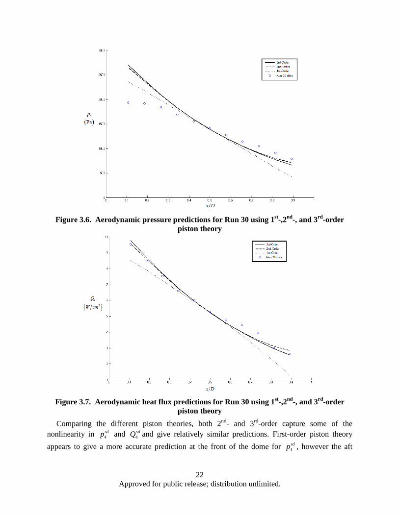
Figure 3.6. Aerodynamic pressure predictions for Run 30 using 1st-,2nd-, and 3rd-order
piston theory
Figure 3.7. Aerodynamic heat flux predictions for Run 30 using 1st-,2nd-, and 3rd-order
piston theory Comparing the different piston theories, both 2nd- and 3rd-order capture some of the
nonlinearity in 4sdp and 4
sdQ and give relatively similar predictions. First-order piston theory appears to give a more accurate prediction at the front of the dome for 4
sdp , however the aft
22 Approved for public release; distribution unlimited.
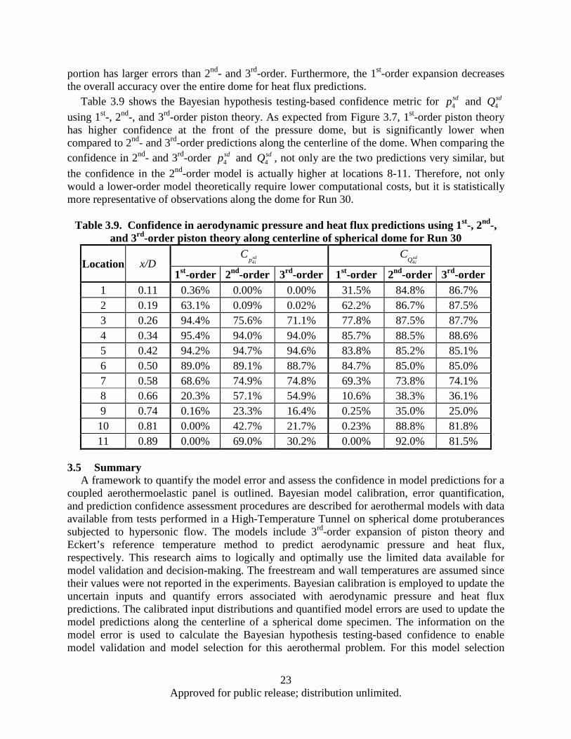
portion has larger errors than 2nd- and 3rd-order. Furthermore, the 1st-order expansion decreases the overall accuracy over the entire dome for heat flux predictions.
Table 3.9 shows the Bayesian hypothesis testing-based confidence metric for 4sdp and 4
sdQ using 1st-, 2nd-, and 3rd-order piston theory. As expected from Figure 3.7, 1st-order piston theory has higher confidence at the front of the pressure dome, but is significantly lower when compared to 2nd- and 3rd-order predictions along the centerline of the dome. When comparing the confidence in 2nd- and 3rd-order 4
sdp and 4sdQ , not only are the two predictions very similar, but
the confidence in the 2nd-order model is actually higher at locations 8-11. Therefore, not only would a lower-order model theoretically require lower computational costs, but it is statistically more representative of observations along the dome for Run 30.
Table 3.9. Confidence in aerodynamic pressure and heat flux predictions using 1st-, 2nd-,
and 3rd-order piston theory along centerline of spherical dome for Run 30
Location x/D 4sd
ipC
4sdiQ
C
1st-order 2nd-order 3rd-order 1st-order 2nd-order 3rd-order 1 0.11 0.36% 0.00% 0.00% 31.5% 84.8% 86.7% 2 0.19 63.1% 0.09% 0.02% 62.2% 86.7% 87.5% 3 0.26 94.4% 75.6% 71.1% 77.8% 87.5% 87.7% 4 0.34 95.4% 94.0% 94.0% 85.7% 88.5% 88.6% 5 0.42 94.2% 94.7% 94.6% 83.8% 85.2% 85.1% 6 0.50 89.0% 89.1% 88.7% 84.7% 85.0% 85.0% 7 0.58 68.6% 74.9% 74.8% 69.3% 73.8% 74.1% 8 0.66 20.3% 57.1% 54.9% 10.6% 38.3% 36.1% 9 0.74 0.16% 23.3% 16.4% 0.25% 35.0% 25.0% 10 0.81 0.00% 42.7% 21.7% 0.23% 88.8% 81.8% 11 0.89 0.00% 69.0% 30.2% 0.00% 92.0% 81.5%
3.5 Summary A framework to quantify the model error and assess the confidence in model predictions for a
coupled aerothermoelastic panel is outlined. Bayesian model calibration, error quantification, and prediction confidence assessment procedures are described for aerothermal models with data available from tests performed in a High-Temperature Tunnel on spherical dome protuberances subjected to hypersonic flow. The models include 3rd-order expansion of piston theory and Eckert’s reference temperature method to predict aerodynamic pressure and heat flux, respectively. This research aims to logically and optimally use the limited data available for model validation and decision-making. The freestream and wall temperatures are assumed since their values were not reported in the experiments. Bayesian calibration is employed to update the uncertain inputs and quantify errors associated with aerodynamic pressure and heat flux predictions. The calibrated input distributions and quantified model errors are used to update the model predictions along the centerline of a spherical dome specimen. The information on the model error is used to calculate the Bayesian hypothesis testing-based confidence to enable model validation and model selection for this aerothermal problem. For this model selection
23 Approved for public release; distribution unlimited.

study among piston theories, it was observed that the highest-order model (3rd-order) did not result in the highest prediction confidence metric.
24 Approved for public release; distribution unlimited.

4 SEGMENTED BAYESIAN MODEL CALIBRATION OF AEROTHERMAL MODELS
Bayesian updating procedures require many evaluations of the models in the Bayesian network, which can be computationally intensive. Most Bayesian calibration work has been done with a single model or multiple models sharing common calibration parameters. Traditionally, as additional experimental data becomes available corresponding to a particular model prediction, recalibration is performed over the entire network. However, for a complex system of models, such as coupled aerothermoelastic response, it becomes imperative to assess the necessity of recalibrating these models simultaneously over the entire network in contrast to updating only the nodes affected by the new data in an isolated, or segmented, manner. In the case of the Bayesian network in this research, it is possible to use the data at the individual nodes to update only the statistically relevant parameters at that node. Thus, a segmented Bayesian model calibration is investigated as a simplified alternative to calibrating all of the models in the complex system simultaneously.
4.1 Bayesian Model Calibration Methodology In this section, the framework to calibrate uncertain model inputs, model discrepancy, and
measurement errors based on the observed values of aerodynamic pressure and heating is presented.
Consider Bayesian calibration of a general model η(ϕ), which contains an uncertain parameters ϕ, with assumed prior distributions π(ϕ), based on prior experience, expert opinion, or historical data. With the observed data y, the distribution of the unknown parameters is updated using Bayes' theorem in Eq. (4.1) .
[ | ( )] ( )( | )[ | ( )] ( )
Pr yyPr y d
η ππη π
=∫
φ φφφ φ φ
(4.1)
Thus, Bayesian updating reduces the uncertainty in parameters ϕ given observations y. Bayes’ theorem is rewritten for the aerodynamic pressure and heat flux predictions and Glass and Hunt experiments in Eq. (4.2).
p Q OS PT ERTp Q
p Q OS PT ERT
[ , | ( ), ( ), ( )] ( )( | ,
[ , | ( ), ( ), ( )] ))
(Pr y y p p Q
y yPr y y p p Q d
ππ
π=
∫φ φ φ φ
φφ φ φ φ φ
(4.2)
The Bayesian network for Eq. (4.2) is constructed using the model and data relationships of the aerothermal models presented in Section 2.1. As previously mentioned, oblique shock relations predict p3 at the leading edge of the test specimen (i.e. flat plate or dome protuberance). For the flat plate, the pressure across the panel is the same as the leading edge pressure, therefore
3 4fp fpp p= . Thus, the flat plate pressure data can be directly applied to the oblique shock
prediction such that fppy = pOS(ϕ) + εOS + )(0,
pyN σ . This isolates the known relationship of the oblique shock prediction to the flat plate, reserving the rigid dome data to calibrate other components of the aerothermal model. Similarly, piston theory and Eckert’s reference temperature models can be related to Glass and Hunt data. In effect, pressure data across the spherical dome ( )p
sdy is applied to calibrate the model discrepancy associated with piston theory
(εPT) and heat flux data ( pQfy , )sd
Qy is used to calibrate the discrepancy associated with Eckert's reference temperature method (εERT ). Note that this description of separating the models and data is used to motivate and explain the segmented calibration approach, however simultaneous
25 Approved for public release; distribution unlimited.
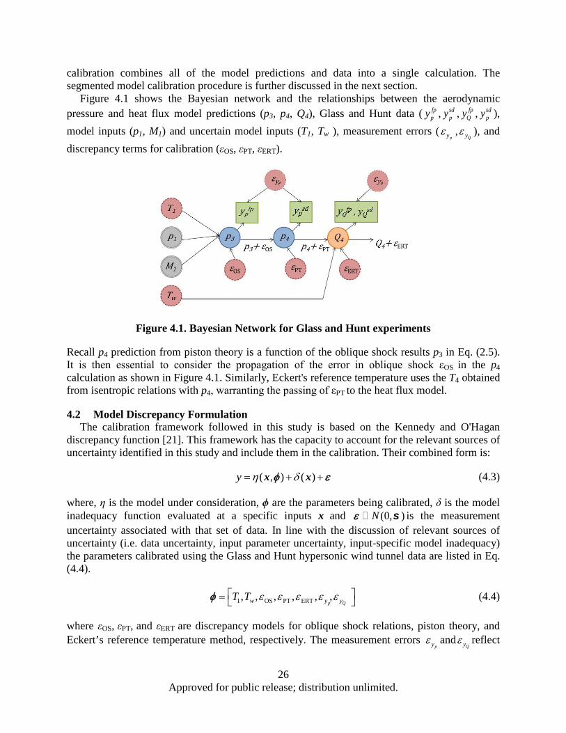
calibration combines all of the model predictions and data into a single calculation. The segmented model calibration procedure is further discussed in the next section.
Figure 4.1 shows the Bayesian network and the relationships between the aerodynamic pressure and heat flux model predictions (p3, p4, Q4), Glass and Hunt data ( fp
py , sdpy , fp
Qy , sdpy ),
model inputs (p1, M1) and uncertain model inputs (T1, Tw ), measurement errors (pyε ,
Qyε ), and discrepancy terms for calibration (εOS, εPT, εERT).
Figure 4.1. Bayesian Network for Glass and Hunt experiments
Recall p4 prediction from piston theory is a function of the oblique shock results p3 in Eq. (2.5). It is then essential to consider the propagation of the error in oblique shock εOS in the p4 calculation as shown in Figure 4.1. Similarly, Eckert's reference temperature uses the T4 obtained from isentropic relations with p4, warranting the passing of εPT to the heat flux model.
4.2 Model Discrepancy Formulation The calibration framework followed in this study is based on the Kennedy and O'Hagan
discrepancy function [21]. This framework has the capacity to account for the relevant sources of uncertainty identified in this study and include them in the calibration. Their combined form is:
( , ) ( )y η δ= + +φ εx x (4.3)
where, η is the model under consideration, ϕ are the parameters being calibrated, δ is the model inadequacy function evaluated at a specific inputs x and )(0,Nε s is the measurement uncertainty associated with that set of data. In line with the discussion of relevant sources of uncertainty (i.e. data uncertainty, input parameter uncertainty, input-specific model inadequacy) the parameters calibrated using the Glass and Hunt hypersonic wind tunnel data are listed in Eq. (4.4).
1 OS PT ERT, , , , , ,p Qyw yT T ε ε ε ε ε = φ (4.4)
where εOS, εPT, and εERT are discrepancy models for oblique shock relations, piston theory, and Eckert’s reference temperature method, respectively. The measurement errors
pyε andQyε reflect
26 Approved for public release; distribution unlimited.
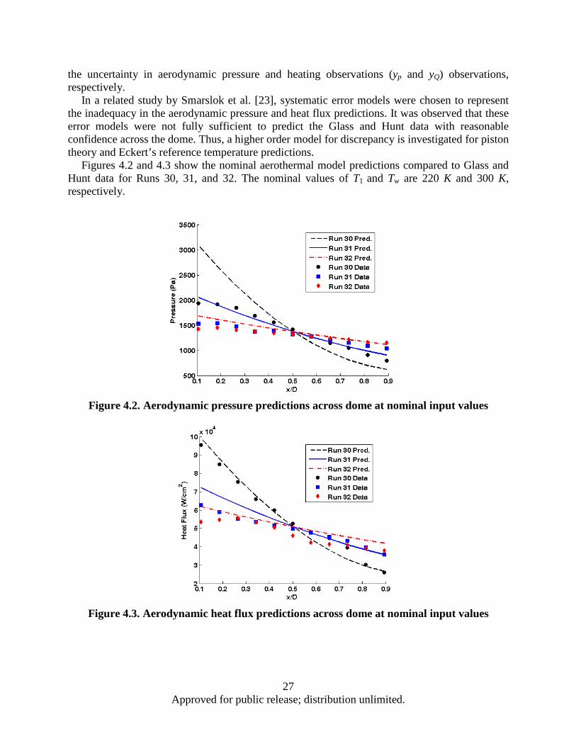
the uncertainty in aerodynamic pressure and heating observations (yp and yQ) observations, respectively.
In a related study by Smarslok et al. [23], systematic error models were chosen to represent the inadequacy in the aerodynamic pressure and heat flux predictions. It was observed that these error models were not fully sufficient to predict the Glass and Hunt data with reasonable confidence across the dome. Thus, a higher order model for discrepancy is investigated for piston theory and Eckert’s reference temperature predictions.
Figures 4.2 and 4.3 show the nominal aerothermal model predictions compared to Glass and Hunt data for Runs 30, 31, and 32. The nominal values of T1 and Tw are 220 K and 300 K, respectively.
Figure 4.2. Aerodynamic pressure predictions across dome at nominal input values
Figure 4.3. Aerodynamic heat flux predictions across dome at nominal input values
27 Approved for public release; distribution unlimited.
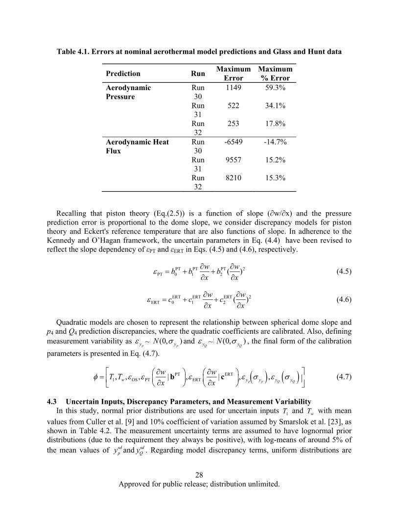
28 Approved for public release; distribution unlimited.
Table 4.1. Errors at nominal aerothermal model predictions and Glass and Hunt data
Prediction Run Maximum
ErrorMaximum % Error
Aerodynamic Pressure
Run 30
1149 59.3%
Run 31
522 34.1%
Run 32
253 17.8%
Aerodynamic Heat Flux
Run 30
-6549 -14.7%
Run 31
9557 15.2%
Run 32
8210 15.3%
Recalling that piston theory (Eq.(2.5)) is a function of slope (∂w/∂x) and the pressure prediction error is proportional to the dome slope, we consider discrepancy models for piston theory and Eckert's reference temperature that are also functions of slope. In adherence to the Kennedy and O’Hagan framework, the uncertain parameters in Eq. (4.4) have been revised to reflect the slope dependency of εPT and εERT in Eqs. (4.5) and (4.6), respectively.
PT PT PT 2PT 0 1 2 ( )
w wb b b
x x
(4.5)
ERT ERT ERT 2ERT 0 1 2 ( )
w wc c c
x x
(4.6)
Quadratic models are chosen to represent the relationship between spherical dome slope and p4 and Q4 prediction discrepancies, where the quadratic coefficients are calibrated. Also, defining measurement variability as (0, )
p py yN and (0, )Q Qy yN , the final form of the calibration
parameters is presented in Eq. (4.7).
PT ERT1 OS PT ERT, , , | , | , ,
p p Q Qyw y y y
w wT T
x x
b c (4.7)
4.3 Uncertain Inputs, Discrepancy Parameters, and Measurement Variability In this study, normal prior distributions are used for uncertain inputs 1T and wT with mean
values from Culler et al. [9] and 10% coefficient of variation assumed by Smarslok et al. [23], as shown in Table 4.2. The measurement uncertainty terms are assumed to have lognormal prior distributions (due to the requirement they always be positive), with log-means of around 5% of the mean values of sd
py and sdQy . Regarding model discrepancy terms, uniform distributions are
~ ~
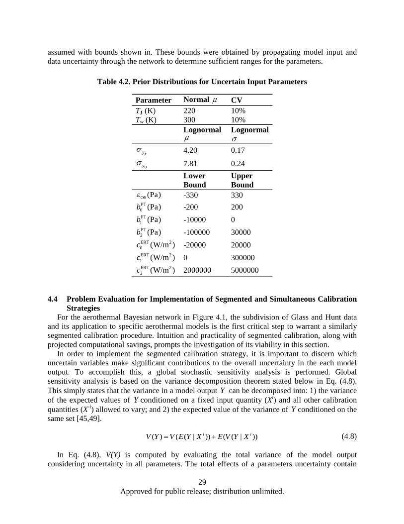
assumed with bounds shown in. These bounds were obtained by propagating model input and data uncertainty through the network to determine sufficient ranges for the parameters.
Table 4.2. Prior Distributions for Uncertain Input Parameters
Parameter Normal µ CV T1 (K) 220 10% Tw (K) 300 10%
Lognormal µ
Lognormal σ
pyσ 4.20 0.17
Qyσ 7.81 0.24
Lower Bound
Upper Bound
OS(Pa)ε -330 330 PT0 (Pa)b -200 200 PT
1 (Pa)b -10000 0 T
2P (Pa)b -100000 30000
20ERT (W/m )c -20000 20000
21ERT (W/m )c 0 300000
22ERT (W/m )c 2000000 5000000
4.4 Problem Evaluation for Implementation of Segmented and Simultaneous Calibration Strategies
For the aerothermal Bayesian network in Figure 4.1, the subdivision of Glass and Hunt data and its application to specific aerothermal models is the first critical step to warrant a similarly segmented calibration procedure. Intuition and practicality of segmented calibration, along with projected computational savings, prompts the investigation of its viability in this section.
In order to implement the segmented calibration strategy, it is important to discern which uncertain variables make significant contributions to the overall uncertainty in the each model output. To accomplish this, a global stochastic sensitivity analysis is performed. Global sensitivity analysis is based on the variance decomposition theorem stated below in Eq. (4.8). This simply states that the variance in a model output Y can be decomposed into: 1) the variance of the expected values of Y conditioned on a fixed input quantity (Xi) and all other calibration quantities (X-i) allowed to vary; and 2) the expected value of the variance of Y conditioned on the same set [45,49].
( ) ( ( | )) ( ( | ))i iV Y V E Y X E V Y X= + (4.8)
In Eq. (4.8), V(Y) is computed by evaluating the total variance of the model output considering uncertainty in all parameters. The total effects of a parameters uncertainty contain
29 Approved for public release; distribution unlimited.
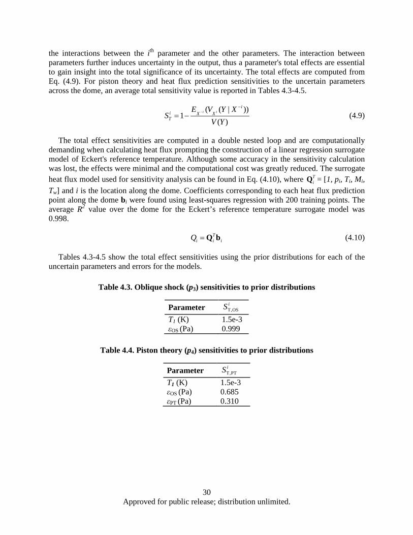
the interactions between the ith parameter and the other parameters. The interaction between parameters further induces uncertainty in the output, thus a parameter's total effects are essential to gain insight into the total significance of its uncertainty. The total effects are computed from Eq. (4.9). For piston theory and heat flux prediction sensitivities to the uncertain parameters across the dome, an average total sensitivity value is reported in Tables 4.3-4.5.
( ( |
1)
))(
i ii
i X XT
E V Y XS
V Y−
−
= − (4.9)
The total effect sensitivities are computed in a double nested loop and are computationally demanding when calculating heat flux prompting the construction of a linear regression surrogate model of Eckert's reference temperature. Although some accuracy in the sensitivity calculation was lost, the effects were minimal and the computational cost was greatly reduced. The surrogate heat flux model used for sensitivity analysis can be found in Eq. (4.10), where T
iQ = [1, pi, Ti, Mi, Tw] and i is the location along the dome. Coefficients corresponding to each heat flux prediction point along the dome bi were found using least-squares regression with 200 training points. The average R2 value over the dome for the Eckert’s reference temperature surrogate model was 0.998.
Ti i iQ = Q b (4.10)
Tables 4.3-4.5 show the total effect sensitivities using the prior distributions for each of the uncertain parameters and errors for the models.
Table 4.3. Oblique shock (p3) sensitivities to prior distributions
Parameter T,OSiS
T1 (K) 1.5e-3 εOS (Pa) 0.999
Table 4.4. Piston theory (p4) sensitivities to prior distributions
Parameter T,PTiS
T1 (K) 1.5e-3 εOS (Pa) 0.685 εPT (Pa) 0.310
30 Approved for public release; distribution unlimited.
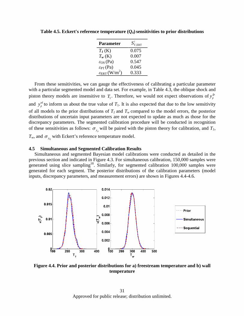
Table 4.5. Eckert's reference temperature (Q4) sensitivities to prior distributions
Parameter T,ERTiS
T1 (K) 0.075 Tw (K) 0.007 εOS (Pa) 0.547 εPT (Pa) 0.045 εERT (W/m2) 0.333
From these sensitivities, we can gauge the effectiveness of calibrating a particular parameter
with a particular segmented model and data set. For example, in Table 4.3, the oblique shock and piston theory models are insensitive to 1T . Therefore, we would not expect observations of fp
py
and dpsy to inform us about the true value of T1. It is also expected that due to the low sensitivity
of all models to the prior distributions of T1 and Tw compared to the model errors, the posterior distributions of uncertain input parameters are not expected to update as much as those for the discrepancy parameters. The segmented calibration procedure will be conducted in recognition of these sensitivities as follows:
pyσ will be paired with the piston theory for calibration, and T1,
Tw, and Qyσ with Eckert’s reference temperature model.
4.5 Simultaneous and Segmented Calibration Results Simultaneous and segmented Bayesian model calibrations were conducted as detailed in the
previous section and indicated in Figure 4.3. For simultaneous calibration, 150,000 samples were generated using slice sampling18. Similarly, for segmented calibration 100,000 samples were generated for each segment. The posterior distributions of the calibration parameters (model inputs, discrepancy parameters, and measurement errors) are shown in Figures 4.4-4.6.
Figure 4.4. Prior and posterior distributions for a) freestream temperature and b) wall
temperature
31 Approved for public release; distribution unlimited.
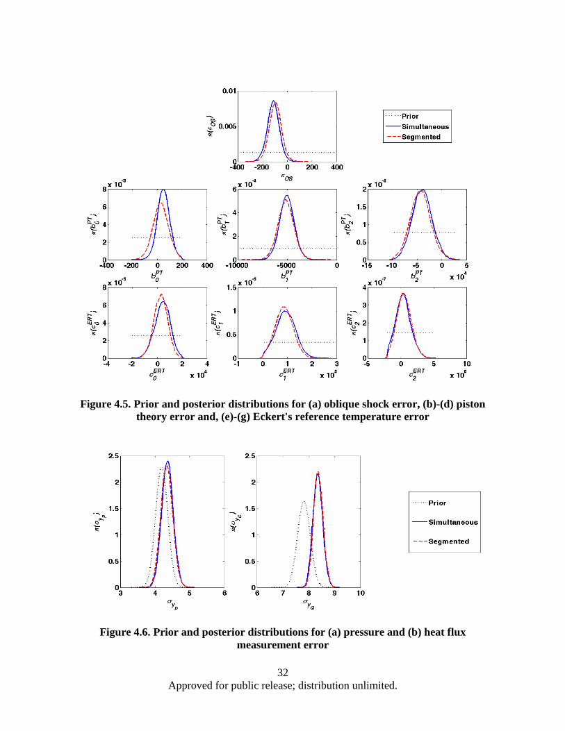
Figure 4.5. Prior and posterior distributions for (a) oblique shock error, (b)-(d) piston
theory error and, (e)-(g) Eckert's reference temperature error
Figure 4.6. Prior and posterior distributions for (a) pressure and (b) heat flux
measurement error
32 Approved for public release; distribution unlimited.
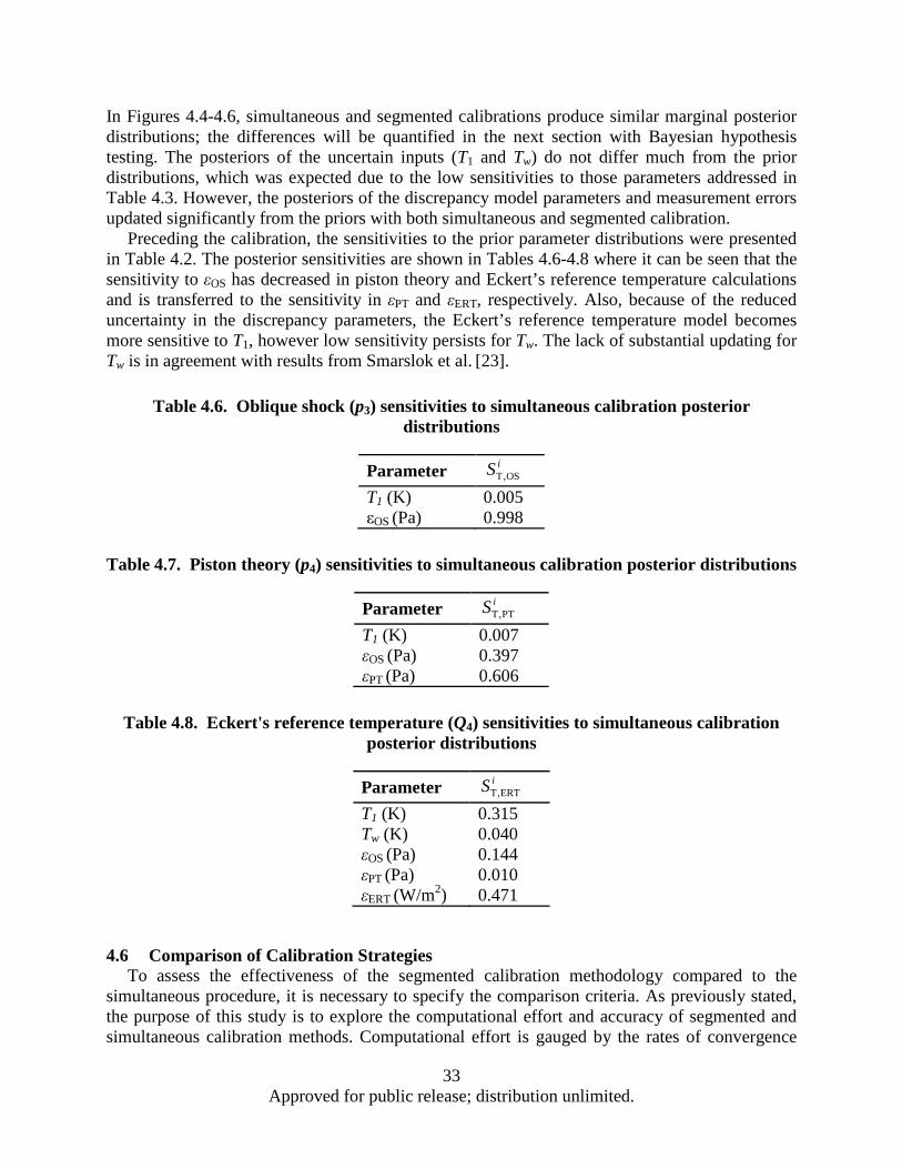
In Figures 4.4-4.6, simultaneous and segmented calibrations produce similar marginal posterior distributions; the differences will be quantified in the next section with Bayesian hypothesis testing. The posteriors of the uncertain inputs (T1 and Tw) do not differ much from the prior distributions, which was expected due to the low sensitivities to those parameters addressed in Table 4.3. However, the posteriors of the discrepancy model parameters and measurement errors updated significantly from the priors with both simultaneous and segmented calibration.
Preceding the calibration, the sensitivities to the prior parameter distributions were presented in Table 4.2. The posterior sensitivities are shown in Tables 4.6-4.8 where it can be seen that the sensitivity to εOS has decreased in piston theory and Eckert’s reference temperature calculations and is transferred to the sensitivity in εPT and εERT, respectively. Also, because of the reduced uncertainty in the discrepancy parameters, the Eckert’s reference temperature model becomes more sensitive to T1, however low sensitivity persists for Tw. The lack of substantial updating for Tw is in agreement with results from Smarslok et al. [23].
Table 4.6. Oblique shock (p3) sensitivities to simultaneous calibration posterior
distributions
Parameter T,OSiS
T1 (K) 0.005 εOS (Pa) 0.998
Table 4.7. Piston theory (p4) sensitivities to simultaneous calibration posterior distributions
Parameter T,PTiS
T1 (K) 0.007 εOS (Pa) 0.397 εPT (Pa) 0.606
Table 4.8. Eckert's reference temperature (Q4) sensitivities to simultaneous calibration
posterior distributions
Parameter T,ERTiS
T1 (K) 0.315 Tw (K) 0.040 εOS (Pa) 0.144 εPT (Pa) 0.010 εERT (W/m2) 0.471
4.6 Comparison of Calibration Strategies To assess the effectiveness of the segmented calibration methodology compared to the
simultaneous procedure, it is necessary to specify the comparison criteria. As previously stated, the purpose of this study is to explore the computational effort and accuracy of segmented and simultaneous calibration methods. Computational effort is gauged by the rates of convergence
33 Approved for public release; distribution unlimited.
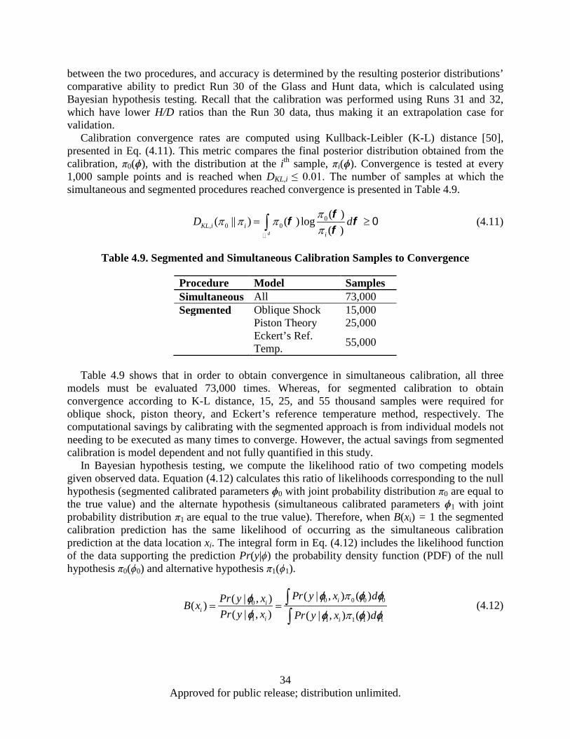
between the two procedures, and accuracy is determined by the resulting posterior distributions’ comparative ability to predict Run 30 of the Glass and Hunt data, which is calculated using Bayesian hypothesis testing. Recall that the calibration was performed using Runs 31 and 32, which have lower H/D ratios than the Run 30 data, thus making it an extrapolation case for validation.
Calibration convergence rates are computed using Kullback-Leibler (K-L) distance [50], presented in Eq. (4.11). This metric compares the final posterior distribution obtained from the calibration, π0(ϕ), with the distribution at the ith sample, πi(ϕ). Convergence is tested at every 1,000 sample points and is reached when DKL,i ≤ 0.01. The number of samples at which the simultaneous and segmented procedures reached convergence is presented in Table 4.9.
0, 0 0
( )( || ) ( ) log( )d
KL i ii
D dππ π ππ
= ≥∫
0ff ff
(4.11)
Table 4.9. Segmented and Simultaneous Calibration Samples to Convergence
Procedure Model Samples Simultaneous All 73,000 Segmented Oblique Shock 15,000 Piston Theory 25,000
Eckert’s Ref. Temp. 55,000
Table 4.9 shows that in order to obtain convergence in simultaneous calibration, all three
models must be evaluated 73,000 times. Whereas, for segmented calibration to obtain convergence according to K-L distance, 15, 25, and 55 thousand samples were required for oblique shock, piston theory, and Eckert’s reference temperature method, respectively. The computational savings by calibrating with the segmented approach is from individual models not needing to be executed as many times to converge. However, the actual savings from segmented calibration is model dependent and not fully quantified in this study.
In Bayesian hypothesis testing, we compute the likelihood ratio of two competing models given observed data. Equation (4.12) calculates this ratio of likelihoods corresponding to the null hypothesis (segmented calibrated parameters ϕ0 with joint probability distribution π0 are equal to the true value) and the alternate hypothesis (simultaneous calibrated parameters ϕ1 with joint probability distribution π1 are equal to the true value). Therefore, when B(xi) = 1 the segmented calibration prediction has the same likelihood of occurring as the simultaneous calibration prediction at the data location xi. The integral form in Eq. (4.12) includes the likelihood function of the data supporting the prediction Pr(y|ϕ) the probability density function (PDF) of the null hypothesis π0(ϕ0) and alternative hypothesis π1(ϕ1).
1 1
0 0 0
1
00
1 1
( | ) ( )( | )( )( |
,
) ( |,
) (, , )ii
i ii
Pr y dPr y xB xPr y x P
x
xr y d
π
π= = ∫
∫φ φ φφ
φ φ φ φ (4.12)
34 Approved for public release; distribution unlimited.

First, Bayesian hypothesis testing was performed separately using flat plate pressure data, spherical dome pressure data, and heat flux data to gauge how well segmented calibration performed for each model. Then, a Bayes factor was computed using all models and data to obtain a combined assessment of segmented calibration. Bayes factors were obtained at each dome location, of which the average, minimum, and maximum are reported for piston theory and Eckert’s reference temperature predictions across the dome. The trends of these individual Bayes factors are values lower than one on the outer dome edges and greater than one closer to the center. Figures 4.7-4.8 show that while the mean predictions are very similar, the uncertainty in the prediction close to the dome center using the segmented posterior distribution is much larger than the uncertainty using simultaneous posteriors, and thus has higher likelihood of containing the data. This accounts for the Bayes factors favoring segmented calibration for predictions near the center of the dome. The results are reported in Table 4.10.
Table 4.10. Bayes Factors for segmented and simultaneous calibration
Model Minimum Maximum Average Oblique Shock - - 0.96 Piston Theory 0.77 1.19 0.92 Eckert’s Ref. Temp. 0.84 1.08 0.94
Combined 0.81 1.89 1.15
Figure 4.7. Pressure predictions across dome from posterior distributions
35 Approved for public release; distribution unlimited.

Figure 4.8. Heat flux predictions across dome from posterior distributions
Table 4.11. Errors in calibrated aerothermal model predictions and Glass and Hunt data
Prediction Maximum Error
Maximum % Error
Aerodynamic Pressure
-191 -10.4%
Aerodynamic Heating -12493 -13.1% Table 4.11 shows the effect of the calibration on the errors in the pressure and heating
prediction compared to the Glass and Hunt data. The maximum percent error in the nominal aerodynamic pressure prediction across the dome for Run 30 is 59.3% which decreased to -10.4% with the calibrated models. Similarly, while the magnitude of the maximum heat flux error for Run 30 increased, the maximum percent error in the heat flux prediction decreased to -13.1% from -14.7% at the nominal prediction.
Another explanation for the differences between predictions using segmented and simultaneous calibration posteriors is that segmented calibration ignores correlation between model error parameters. These correlations are significant in the simultaneous posterior samples and are listed in Table 4.12. For example, when εOS is small the first term in εPT is large in the simultaneous posterior samples. However, for predictions from the segmented calibration posteriors, we select samples of εOS, εPT , and εERT independently, resulting in a larger variance in prediction. Table 4.12 lists the most significant correlations between εOS, terms in εPT and terms in εERT.
36 Approved for public release; distribution unlimited.
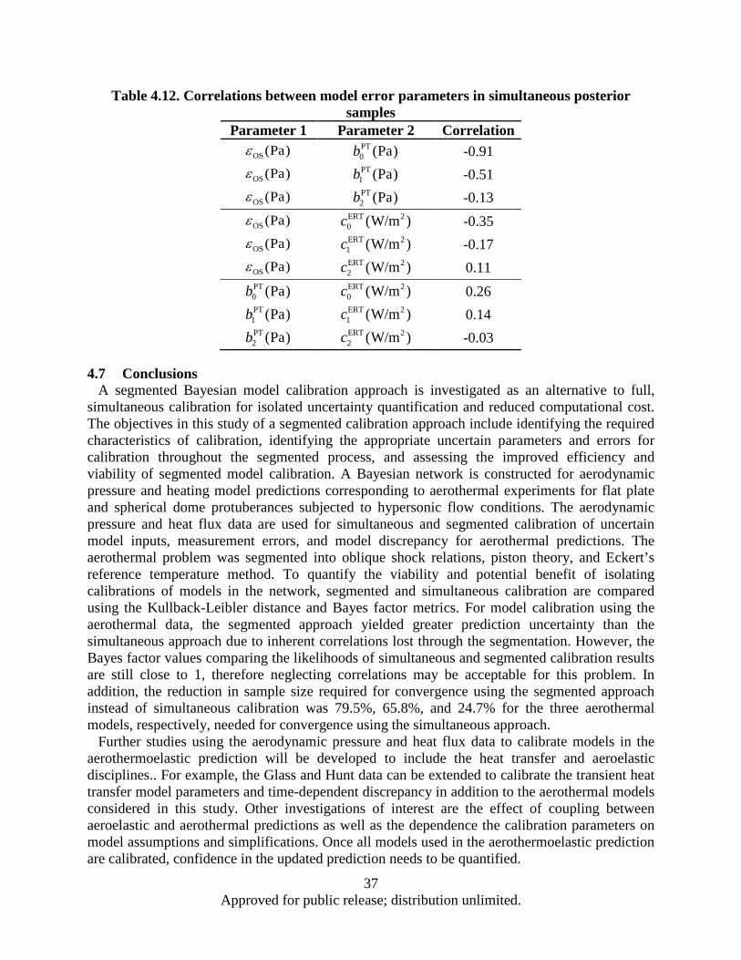
Table 4.12. Correlations between model error parameters in simultaneous posterior samples
Parameter 1 Parameter 2 Correlation OS(Pa)ε PT
0 (Pa)b -0.91
OS(Pa)ε T1P (Pa)b -0.51
OS(Pa)ε T2P (Pa)b -0.13
OS(Pa)ε 2ERT
0 (W/m )c -0.35
OS(Pa)ε 2
1ERT (W/m )c -0.17
OS(Pa)ε 2
2ERT (W/m )c 0.11
PT0 (Pa)b
20ERT (W/m )c 0.26
T1P (Pa)b
21ERT (W/m )c 0.14
T2P (Pa)b
22ERT (W/m )c -0.03
4.7 Conclusions A segmented Bayesian model calibration approach is investigated as an alternative to full,
simultaneous calibration for isolated uncertainty quantification and reduced computational cost. The objectives in this study of a segmented calibration approach include identifying the required characteristics of calibration, identifying the appropriate uncertain parameters and errors for calibration throughout the segmented process, and assessing the improved efficiency and viability of segmented model calibration. A Bayesian network is constructed for aerodynamic pressure and heating model predictions corresponding to aerothermal experiments for flat plate and spherical dome protuberances subjected to hypersonic flow conditions. The aerodynamic pressure and heat flux data are used for simultaneous and segmented calibration of uncertain model inputs, measurement errors, and model discrepancy for aerothermal predictions. The aerothermal problem was segmented into oblique shock relations, piston theory, and Eckert’s reference temperature method. To quantify the viability and potential benefit of isolating calibrations of models in the network, segmented and simultaneous calibration are compared using the Kullback-Leibler distance and Bayes factor metrics. For model calibration using the aerothermal data, the segmented approach yielded greater prediction uncertainty than the simultaneous approach due to inherent correlations lost through the segmentation. However, the Bayes factor values comparing the likelihoods of simultaneous and segmented calibration results are still close to 1, therefore neglecting correlations may be acceptable for this problem. In addition, the reduction in sample size required for convergence using the segmented approach instead of simultaneous calibration was 79.5%, 65.8%, and 24.7% for the three aerothermal models, respectively, needed for convergence using the simultaneous approach.
Further studies using the aerodynamic pressure and heat flux data to calibrate models in the aerothermoelastic prediction will be developed to include the heat transfer and aeroelastic disciplines.. For example, the Glass and Hunt data can be extended to calibrate the transient heat transfer model parameters and time-dependent discrepancy in addition to the aerothermal models considered in this study. Other investigations of interest are the effect of coupling between aeroelastic and aerothermal predictions as well as the dependence the calibration parameters on model assumptions and simplifications. Once all models used in the aerothermoelastic prediction are calibrated, confidence in the updated prediction needs to be quantified.
37 Approved for public release; distribution unlimited.
5 BAYESIAN CALIBRATION OF AEROTHERMAL MODELS USING TIME-DEPENDENT DATA
In this section, the Bayesian calibration approach for using observed aerodynamic pressure and temperature measurements to reduce uncertainty in the aerothermal predictions is presented. Uncertain model inputs, model discrepancy, and measurement errors are considered for calibration. Additionally, the dynamic Bayesian network is constructed for the coupled, transient aerothermal problem and two implementations of time-dependent discrepancy models are compared and discussed. Prior distributions for discrepancy model parameters in Eckert’s reference temperature and linear heat transfer are presented. A direct calibration performance comparison between global and incremental discrepancy application at the dome midpoint follows using a time-dependent Bayes’ factor for model selection. The selected discrepancy treatment is applied to the full dome for validation.
5.1 Bayesian Model Calibration Methodology for Time-Dependent Data Consider Bayesian calibration of a model η(ϕ), which contains an uncertain parameters ϕ
composed of model inputs, discrepancy parameters, or measurement errors with assumed prior distributions π(ϕ), based on prior experience, expert opinion, or historical data. With the observed data y, the distribution of the unknown parameters is updated using continuous Bayes' theorem in Eq. (5.1).
𝜋𝜋(𝝓𝝓|𝑦𝑦) =Pr[𝑦𝑦|𝜂𝜂(𝝓𝝓)]𝜋𝜋(𝝓𝝓)
∫ 𝑃𝑃𝑃𝑃[𝑦𝑦|𝜂𝜂(𝝓𝝓)]𝜋𝜋(𝝓𝝓)𝑑𝑑𝝓𝝓 (5.1)
Thus, Bayesian updating reduces the uncertainty in parameters ϕ given observations y. Bayes’ theorem is rewritten for the aerodynamic pressure, heat flux, and heat transfer predictions (from piston theory, Eckert’s reference temperature, and linear heat transfer, respectively) and Glass and Hunt data in Eq. (2.8). Recall from Section 2, the heat flux data reported by Glass and Hunt was used to extract the temperature history across the panel. For this reason, only the derived temperature history and pressure can be used in the Bayesian network.
𝜋𝜋𝝓𝝓𝑦𝑦𝑝𝑝,𝑦𝑦𝑇𝑇 =Pr𝑦𝑦𝑝𝑝,𝑦𝑦𝑇𝑇|𝑝𝑝𝑃𝑃𝑇𝑇(𝝓𝝓),𝑄𝑄𝐸𝐸𝐸𝐸𝑇𝑇(𝝓𝝓),𝑇𝑇𝐻𝐻𝑇𝑇(𝝓𝝓)𝜋𝜋(𝝓𝝓)
∫ Pr𝑦𝑦𝑝𝑝,𝑦𝑦𝑇𝑇|𝑝𝑝𝑃𝑃𝑇𝑇(𝝓𝝓),𝑄𝑄𝐸𝐸𝐸𝐸𝑇𝑇(𝝓𝝓),𝑇𝑇𝐻𝐻𝑇𝑇(𝝓𝝓)𝜋𝜋(𝝓𝝓)𝑑𝑑𝝓𝝓 (5.2)
The Bayesian network for Eq. (5.2) is constructed using the relationships between the
aerothermal models and available Glass and Hunt data presented in Section 2.2. Figure 5.1 shows the Bayesian network and the relationships between the aerodynamic pressure, heat flux, and heat transfer models (p4, Q4, Tw), aerothermal data (yp, yT), model inputs (p1, M1, Tw,0), measurement errors (𝜀𝜀𝑦𝑦𝑇𝑇,𝜀𝜀𝑦𝑦𝑝𝑝), and discrepancy terms for calibration (εPT, εERT, εHT).
38 Approved for public release; distribution unlimited.
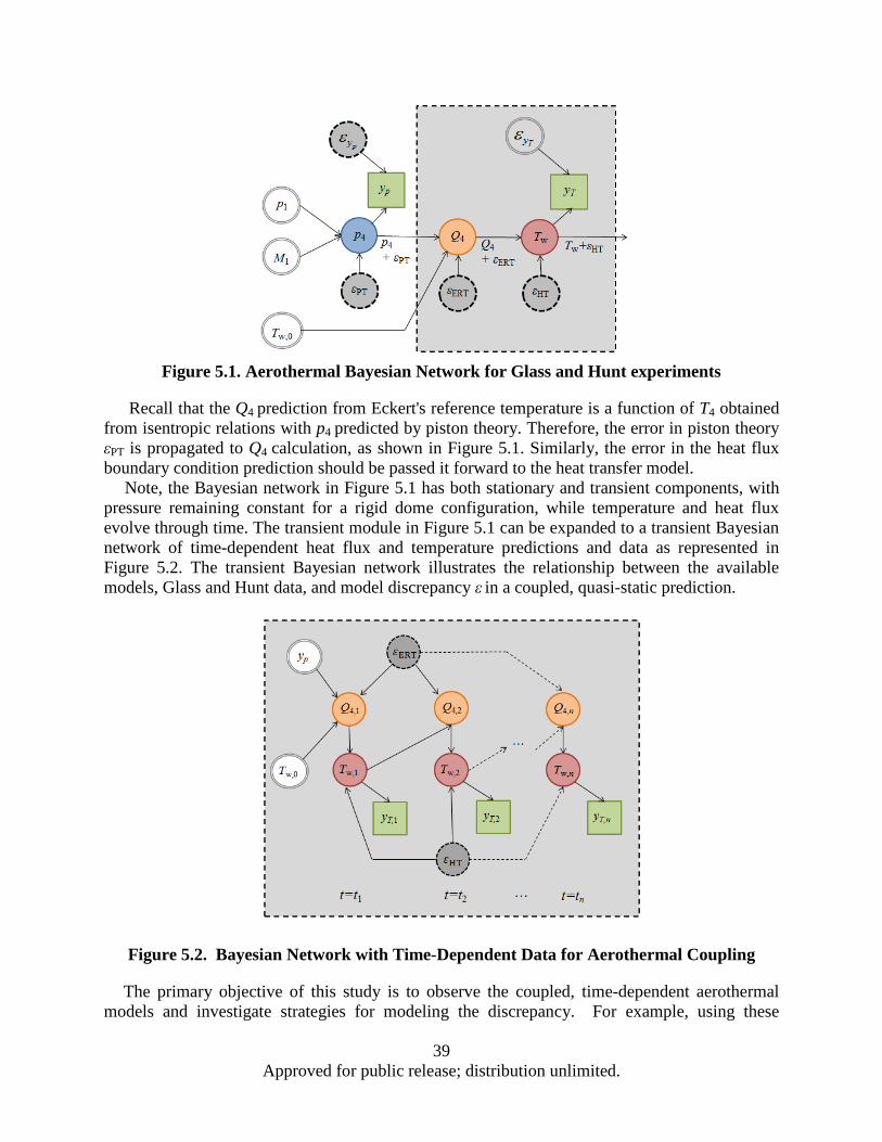
Figure 5.1. Aerothermal Bayesian Network for Glass and Hunt experiments
Recall that the Q4 prediction from Eckert's reference temperature is a function of T4 obtained from isentropic relations with p4 predicted by piston theory. Therefore, the error in piston theory εPT is propagated to Q4 calculation, as shown in Figure 5.1. Similarly, the error in the heat flux boundary condition prediction should be passed it forward to the heat transfer model.
Note, the Bayesian network in Figure 5.1 has both stationary and transient components, with pressure remaining constant for a rigid dome configuration, while temperature and heat flux evolve through time. The transient module in Figure 5.1 can be expanded to a transient Bayesian network of time-dependent heat flux and temperature predictions and data as represented in Figure 5.2. The transient Bayesian network illustrates the relationship between the available models, Glass and Hunt data, and model discrepancy ε in a coupled, quasi-static prediction.
Figure 5.2. Bayesian Network with Time-Dependent Data for Aerothermal Coupling
The primary objective of this study is to observe the coupled, time-dependent aerothermal models and investigate strategies for modeling the discrepancy. For example, using these
39 Approved for public release; distribution unlimited.
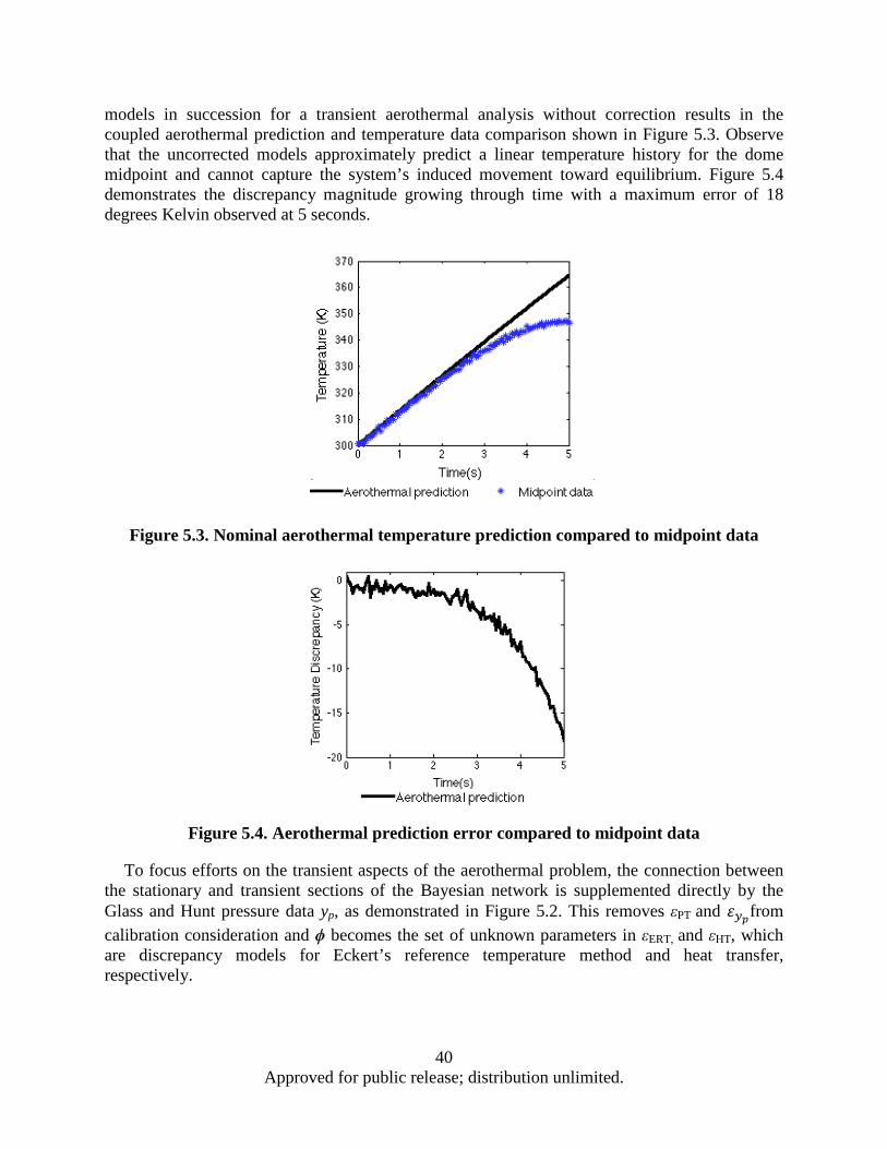
models in succession for a transient aerothermal analysis without correction results in the coupled aerothermal prediction and temperature data comparison shown in Figure 5.3. Observe that the uncorrected models approximately predict a linear temperature history for the dome midpoint and cannot capture the system’s induced movement toward equilibrium. Figure 5.4 demonstrates the discrepancy magnitude growing through time with a maximum error of 18 degrees Kelvin observed at 5 seconds.
Figure 5.3. Nominal aerothermal temperature prediction compared to midpoint data
Figure 5.4. Aerothermal prediction error compared to midpoint data
To focus efforts on the transient aspects of the aerothermal problem, the connection between the stationary and transient sections of the Bayesian network is supplemented directly by the Glass and Hunt pressure data yp, as demonstrated in Figure 5.2. This removes εPT and 𝜀𝜀𝑦𝑦𝑝𝑝from calibration consideration and ϕ becomes the set of unknown parameters in εERT, and εHT, which are discrepancy models for Eckert’s reference temperature method and heat transfer, respectively.
40 Approved for public release; distribution unlimited.
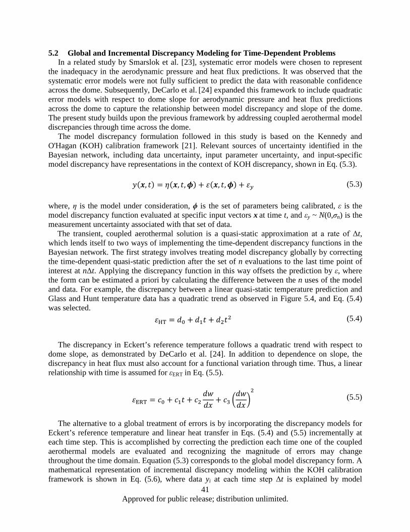
5.2 Global and Incremental Discrepancy Modeling for Time-Dependent Problems In a related study by Smarslok et al. [23], systematic error models were chosen to represent
the inadequacy in the aerodynamic pressure and heat flux predictions. It was observed that the systematic error models were not fully sufficient to predict the data with reasonable confidence across the dome. Subsequently, DeCarlo et al. [24] expanded this framework to include quadratic error models with respect to dome slope for aerodynamic pressure and heat flux predictions across the dome to capture the relationship between model discrepancy and slope of the dome. The present study builds upon the previous framework by addressing coupled aerothermal model discrepancies through time across the dome.
The model discrepancy formulation followed in this study is based on the Kennedy and O'Hagan (KOH) calibration framework [21]. Relevant sources of uncertainty identified in the Bayesian network, including data uncertainty, input parameter uncertainty, and input-specific model discrepancy have representations in the context of KOH discrepancy, shown in Eq. (5.3).
𝑦𝑦(𝒙𝒙, 𝑡𝑡) = 𝜂𝜂(𝒙𝒙, 𝑡𝑡,𝝓𝝓) + 𝜀𝜀(𝒙𝒙, 𝑡𝑡,𝝓𝝓) + 𝜀𝜀𝑦𝑦 (5.3)
where, η is the model under consideration, ϕ is the set of parameters being calibrated, ε is the model discrepancy function evaluated at specific input vectors x at time t, and εy ~ N(0,σn) is the measurement uncertainty associated with that set of data.
The transient, coupled aerothermal solution is a quasi-static approximation at a rate of Δt, which lends itself to two ways of implementing the time-dependent discrepancy functions in the Bayesian network. The first strategy involves treating model discrepancy globally by correcting the time-dependent quasi-static prediction after the set of n evaluations to the last time point of interest at nΔt. Applying the discrepancy function in this way offsets the prediction by ε, where the form can be estimated a priori by calculating the difference between the n uses of the model and data. For example, the discrepancy between a linear quasi-static temperature prediction and Glass and Hunt temperature data has a quadratic trend as observed in Figure 5.4, and Eq. (5.4) was selected.
𝜀𝜀HT = 𝑑𝑑0 + 𝑑𝑑1𝑡𝑡 + 𝑑𝑑2𝑡𝑡2 (5.4)
The discrepancy in Eckert’s reference temperature follows a quadratic trend with respect to
dome slope, as demonstrated by DeCarlo et al. [24]. In addition to dependence on slope, the discrepancy in heat flux must also account for a functional variation through time. Thus, a linear relationship with time is assumed for εERT in Eq. (5.5).
𝜀𝜀ERT = 𝑐𝑐0 + 𝑐𝑐1𝑡𝑡 + 𝑐𝑐2𝑑𝑑𝑑𝑑𝑑𝑑𝑑𝑑
+ 𝑐𝑐3 𝑑𝑑𝑑𝑑𝑑𝑑𝑑𝑑
2
(5.5)
The alternative to a global treatment of errors is by incorporating the discrepancy models for Eckert’s reference temperature and linear heat transfer in Eqs. (5.4) and (5.5) incrementally at each time step. This is accomplished by correcting the prediction each time one of the coupled aerothermal models are evaluated and recognizing the magnitude of errors may change throughout the time domain. Equation (5.3) corresponds to the global model discrepancy form. A mathematical representation of incremental discrepancy modeling within the KOH calibration framework is shown in Eq. (5.6), where data yi at each time step Δt is explained by model
41 Approved for public release; distribution unlimited.
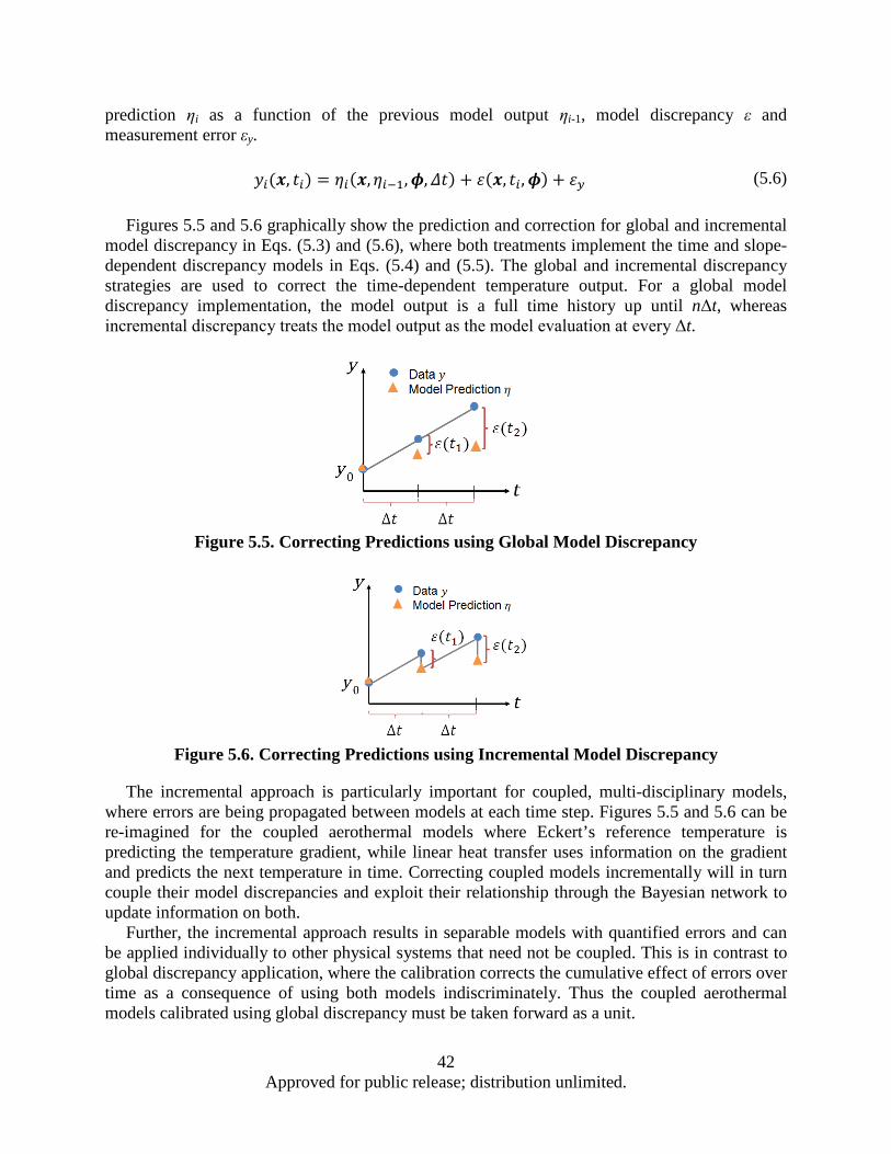
prediction ηi as a function of the previous model output ηi-1, model discrepancy ε and measurement error εy.
𝑦𝑦𝑖𝑖(𝒙𝒙, 𝑡𝑡𝑖𝑖) = 𝜂𝜂𝑖𝑖(𝒙𝒙,𝜂𝜂𝑖𝑖−1,𝝓𝝓,𝛥𝛥𝑡𝑡) + 𝜀𝜀(𝒙𝒙, 𝑡𝑡𝑖𝑖,𝝓𝝓) + 𝜀𝜀𝑦𝑦 (5.6) Figures 5.5 and 5.6 graphically show the prediction and correction for global and incremental model discrepancy in Eqs. (5.3) and (5.6), where both treatments implement the time and slope-dependent discrepancy models in Eqs. (5.4) and (5.5). The global and incremental discrepancy strategies are used to correct the time-dependent temperature output. For a global model discrepancy implementation, the model output is a full time history up until nΔt, whereas incremental discrepancy treats the model output as the model evaluation at every Δt.
Figure 5.5. Correcting Predictions using Global Model Discrepancy
Figure 5.6. Correcting Predictions using Incremental Model Discrepancy
The incremental approach is particularly important for coupled, multi-disciplinary models, where errors are being propagated between models at each time step. Figures 5.5 and 5.6 can be re-imagined for the coupled aerothermal models where Eckert’s reference temperature is predicting the temperature gradient, while linear heat transfer uses information on the gradient and predicts the next temperature in time. Correcting coupled models incrementally will in turn couple their model discrepancies and exploit their relationship through the Bayesian network to update information on both.
Further, the incremental approach results in separable models with quantified errors and can be applied individually to other physical systems that need not be coupled. This is in contrast to global discrepancy application, where the calibration corrects the cumulative effect of errors over time as a consequence of using both models indiscriminately. Thus the coupled aerothermal models calibrated using global discrepancy must be taken forward as a unit.
42 Approved for public release; distribution unlimited.

Note, the incremental and global discrepancy functions have the same form, however the calibrated coefficients for heat transfer discrepancy (d0, d1, d2) will be different depending on the strategy implemented. Since the incremental discrepancy strategy corrects the prediction at each time step, then the magnitude of the discrepancy at a given time t is less than that of the global discrepancy. Section 5.3 will list appropriate prior distributions for Bayesian calibration of the model discrepancy parameters, compare the incremental and global error application approaches through both sensitivity analyses and calibration, and select an error treatment to apply to the full dome for validation. Section 5.3 will list appropriate prior distributions for Bayesian calibration of the model discrepancy parameters.
5.3 Prior Uncertainty and Discrepancy Implementation Selection Prior distributions for parameters of εERT and εHT using both incremental and global treatments
of model discrepancy are shown in Table 5.1. All prior distributions are uniform distributions with lower and upper bounds specified. Prior distribution ranges were chosen by passing the maximum likelihood values of the other parameters through the transient aerothermal models and comparing nominal predictions to the Glass and Hunt data.
Table 5.1. Prior Distributions for Discrepancy Model Parameters
Parameter
Incremental Global Lower Bound
Upper Bound
Lower Bound
Upper Bound
c0 (W/cm2) -0.5 0.3 -0.5 0.3 c1 (W/cm2t) -0.1 0.1 -0.1 0.1 c2 (W/cm2) -100 200 -100 200 c3 (W/cm2) -1000 1000 -1000 1000 d0 (K) -0.1 0.1 -3 3 d1 (K/t) -0.1 0.1 -4 3 d2 (K/t2) -0.1 0.1 -2 1
Both discrepancy treatments are applied through the dynamic Bayesian network and used to
calibrate discrepancy models at the midpoint of the dome. The calibration domain consists of time-dependent temperature data up until 4 seconds into Runs 30, 31, and 32 of Glass and Hunt turbulent flow experiments. The remaining second of temperature data is used for decision-making. For this comparison only the dome midpoint temperature data (where 𝜕𝜕𝑑𝑑/𝜕𝜕𝑑𝑑 is zero) is considered; the quadratic slope terms have no effect in this single point calibration.
Figures 5.7 and 5.8 show the calibrated incremental and global discrepancy models for heat transfer through time. Note that both models have similar quadratic trends, however incremental discrepancy mean predictions are on average two orders of magnitude less than those of the global discrepancy mean prediction. Further, the uncertainty in the global discrepancy model is growing, whereas the uncertainty in the incremental discrepancy model is relatively constant.
43 Approved for public release; distribution unlimited.

Figure 5.7. Calibrated global discrepancy model through time
Figure 5.8. Calibrated global discrepancy model through time
The predictions from both calibrated discrepancy models at the dome midpoint decides which should be used for the remainder of the dome points. The calibrated discrepancy models are propagated forward through the network for Runs 30, 31, and 32 predictions.
Figure 5.9. Calibrated aerothermal model predictions using global discrepancy application
44 Approved for public release; distribution unlimited.
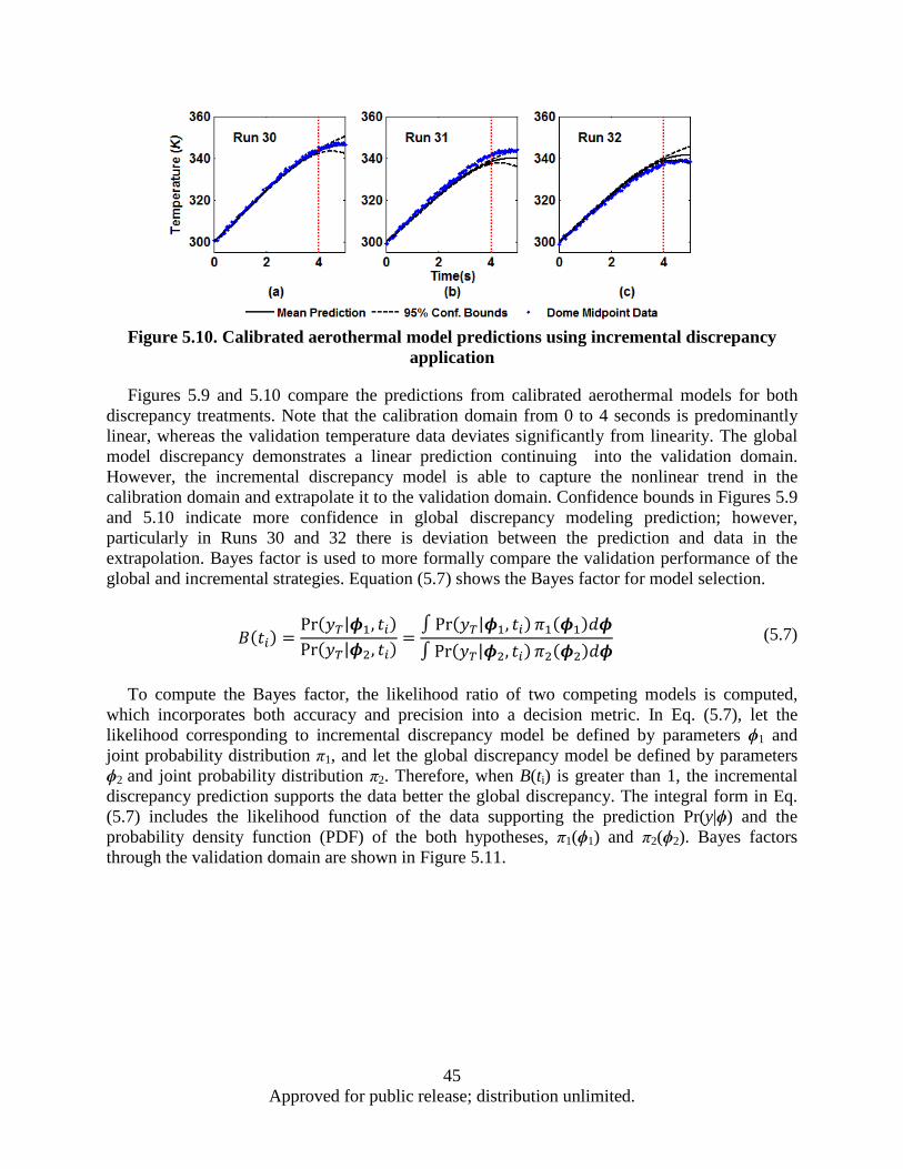
Figure 5.10. Calibrated aerothermal model predictions using incremental discrepancy application
Figures 5.9 and 5.10 compare the predictions from calibrated aerothermal models for both discrepancy treatments. Note that the calibration domain from 0 to 4 seconds is predominantly linear, whereas the validation temperature data deviates significantly from linearity. The global model discrepancy demonstrates a linear prediction continuing into the validation domain. However, the incremental discrepancy model is able to capture the nonlinear trend in the calibration domain and extrapolate it to the validation domain. Confidence bounds in Figures 5.9 and 5.10 indicate more confidence in global discrepancy modeling prediction; however, particularly in Runs 30 and 32 there is deviation between the prediction and data in the extrapolation. Bayes factor is used to more formally compare the validation performance of the global and incremental strategies. Equation (5.7) shows the Bayes factor for model selection.
𝐵𝐵(𝑡𝑡𝑖𝑖) =Pr(𝑦𝑦𝑇𝑇|𝝓𝝓1, 𝑡𝑡𝑖𝑖)Pr(𝑦𝑦𝑇𝑇|𝝓𝝓2, 𝑡𝑡𝑖𝑖)
=∫ Pr(𝑦𝑦𝑇𝑇|𝝓𝝓1, 𝑡𝑡𝑖𝑖)𝜋𝜋1(𝝓𝝓1)𝑑𝑑𝝓𝝓∫ Pr(𝑦𝑦𝑇𝑇|𝝓𝝓2, 𝑡𝑡𝑖𝑖)𝜋𝜋2(𝝓𝝓2)𝑑𝑑𝝓𝝓
(5.7)
To compute the Bayes factor, the likelihood ratio of two competing models is computed,
which incorporates both accuracy and precision into a decision metric. In Eq. (5.7), let the likelihood corresponding to incremental discrepancy model be defined by parameters ϕ1 and joint probability distribution π1, and let the global discrepancy model be defined by parameters ϕ2 and joint probability distribution π2. Therefore, when B(ti) is greater than 1, the incremental discrepancy prediction supports the data better the global discrepancy. The integral form in Eq. (5.7) includes the likelihood function of the data supporting the prediction Pr(y|ϕ) and the probability density function (PDF) of the both hypotheses, π1(ϕ1) and π2(ϕ2). Bayes factors through the validation domain are shown in Figure 5.11.
45 Approved for public release; distribution unlimited.
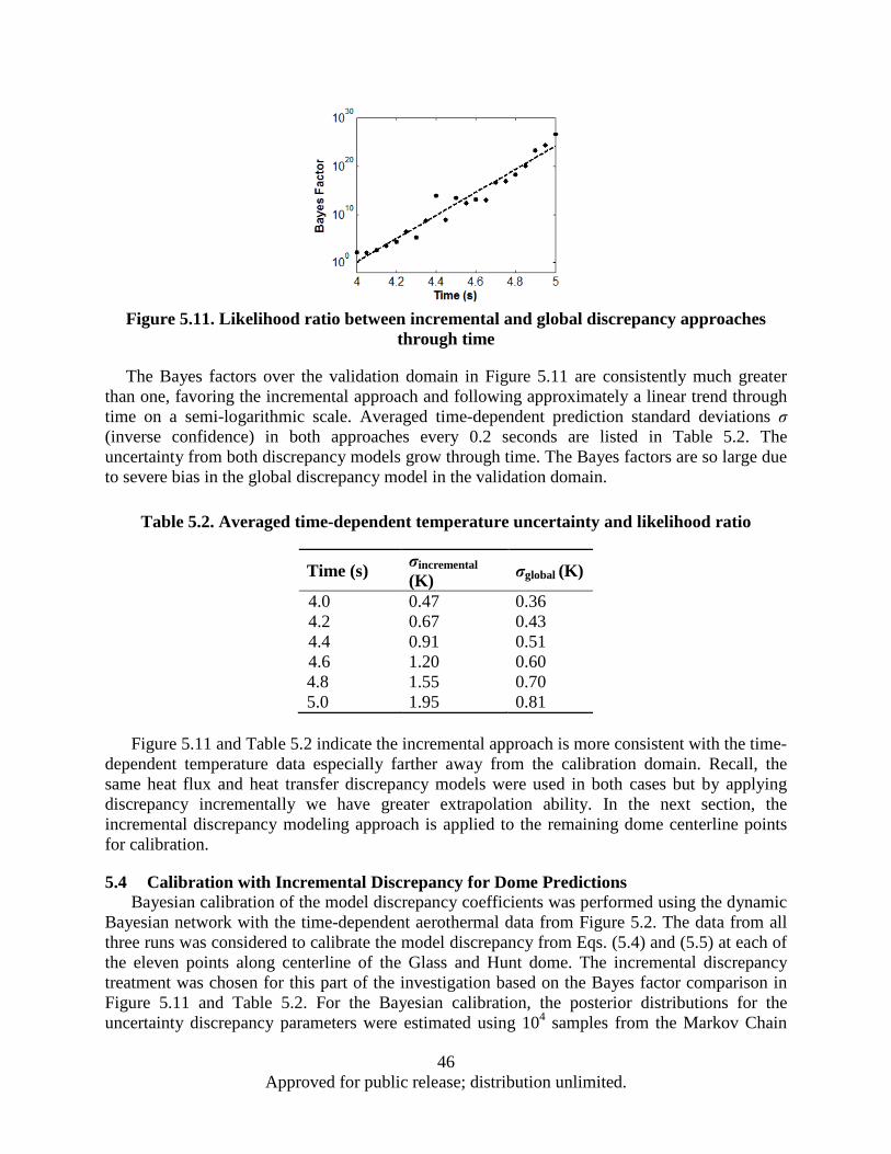
Figure 5.11. Likelihood ratio between incremental and global discrepancy approaches
through time
The Bayes factors over the validation domain in Figure 5.11 are consistently much greater than one, favoring the incremental approach and following approximately a linear trend through time on a semi-logarithmic scale. Averaged time-dependent prediction standard deviations σ (inverse confidence) in both approaches every 0.2 seconds are listed in Table 5.2. The uncertainty from both discrepancy models grow through time. The Bayes factors are so large due to severe bias in the global discrepancy model in the validation domain.
Table 5.2. Averaged time-dependent temperature uncertainty and likelihood ratio
Time (s) σincremental (K) σglobal (K)
4.0 0.47 0.36 4.2 0.67 0.43 4.4 0.91 0.51 4.6 1.20 0.60 4.8 1.55 0.70 5.0 1.95 0.81
Figure 5.11 and Table 5.2 indicate the incremental approach is more consistent with the time-
dependent temperature data especially farther away from the calibration domain. Recall, the same heat flux and heat transfer discrepancy models were used in both cases but by applying discrepancy incrementally we have greater extrapolation ability. In the next section, the incremental discrepancy modeling approach is applied to the remaining dome centerline points for calibration.
5.4 Calibration with Incremental Discrepancy for Dome Predictions Bayesian calibration of the model discrepancy coefficients was performed using the dynamic
Bayesian network with the time-dependent aerothermal data from Figure 5.2. The data from all three runs was considered to calibrate the model discrepancy from Eqs. (5.4) and (5.5) at each of the eleven points along centerline of the Glass and Hunt dome. The incremental discrepancy treatment was chosen for this part of the investigation based on the Bayes factor comparison in Figure 5.11 and Table 5.2. For the Bayesian calibration, the posterior distributions for the uncertainty discrepancy parameters were estimated using 104 samples from the Markov Chain
46 Approved for public release; distribution unlimited.

Monte Carlo (MCMC) algorithm called slice sampling. Figures 5.12-5.14 show the corrected predictions using the incremental discrepancy approach for Runs 30, 31 and 32, respectively. For all three cases, the predictions shown at 1 and 3 seconds are in the calibration domain, whereas 5 seconds is in the validation domain.
Figure 5.12. Calibrated Run 30 prediction across dome at 1, 3, and 5 seconds
Figure 5.13. Calibrated Run 31 prediction across dome at 1, 3, and 5 seconds
Figure 5.14. Calibrated Run 32 prediction across dome at 1, 3, and 5 seconds
Figures 5.12-5.14 show small model discrepancy in the calibration time domain (t = 1s and 3s) and growing extrapolation uncertainty in the validation domain (t = 5s). This is analogous to Figure 5.10, where uncertainty increased when predicting beyond 4 seconds. Table 5.3 lists the average uncertainty in the calibrated predictions for each experiment. Run 31 shows the most
47 Approved for public release; distribution unlimited.
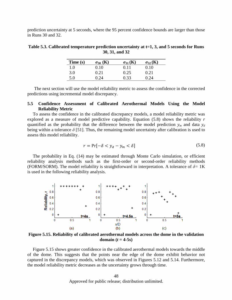
prediction uncertainty at 5 seconds, where the 95 percent confidence bounds are larger than those in Runs 30 and 32. Table 5.3. Calibrated temperature prediction uncertainty at t=1, 3, and 5 seconds for Runs
30, 31, and 32
Time (s) σ30 (K) σ31 (K) σ32 (K) 1.0 0.10 0.11 0.10 3.0 0.21 0.25 0.21 5.0 0.24 0.33 0.24
The next section will use the model reliability metric to assess the confidence in the corrected
predictions using incremental model discrepancy.
5.5 Confidence Assessment of Calibrated Aerothermal Models Using the Model Reliability Metric
To assess the confidence in the calibrated discrepancy models, a model reliability metric was explored as a measure of model predictive capability. Equation (5.8) shows the reliability r quantified as the probability that the difference between the model prediction ym and data yd being within a tolerance δ [51]. Thus, the remaining model uncertainty after calibration is used to assess this model reliability.
𝑃𝑃 = Pr [−𝛿𝛿 < 𝑦𝑦𝑑𝑑 − 𝑦𝑦𝑚𝑚 < 𝛿𝛿] (5.8)
The probability in Eq. (14) may be estimated through Monte Carlo simulation, or efficient reliability analysis methods such as the first-order or second-order reliability methods (FORM/SORM). The model reliability is straightforward in interpretation. A tolerance of δ= 1K is used in the following reliability analysis.
Figure 5.15. Reliability of calibrated aerothermal models across the dome in the validation
domain (t = 4-5s)
Figure 5.15 shows greater confidence in the calibrated aerothermal models towards the middle of the dome. This suggests that the points near the edge of the dome exhibit behavior not captured in the discrepancy models, which was observed in Figures 5.12 and 5.14. Furthermore, the model reliability metric decreases as the uncertainty grows through time.
48 Approved for public release; distribution unlimited.

5.6 Summary and Conclusions This research is part of a series of investigations on quantifying the confidence in coupled
aerothermal elastic models for hypersonic aircraft structures. Bayesian model calibration methods were extended for a coupled, time-dependent problem. A dynamic Bayesian network for coupled aerothermal models (including, aerodynamic pressure and heat flux, and transient heat transfer) and time-dependent data was developed. Bayesian model calibration was performed for model discrepancy using time-dependent temperature data from historic aerothermal experiments conducted at NASA's 8-foot High-Temperature Tunnel. Two ways to implement the dynamic model errors were investigated, and it was determined that applying incremental errors through time supplied the model with greater extrapolation ability. Finally, the incremental discrepancy strategy was extended to calibrate the dynamic aerothermal error models at eleven points along the dome centerline. The model reliability metric for model validation was used to assess spatial and temporal confidence in the aerothermal predictions across the dome. Confidence in calibrated aerothermal discrepancy models increased towards the dome midpoint and over time through the validation domain.
49 Approved for public release; distribution unlimited.

6 INVESTIGATING MODEL UNCERTAINTY IN AEROELASTIC RESPONSE OF THIN PANELS
Recent research efforts have focused on the development of computational frameworks enabling the prediction of coupled fluid-thermal-structural response [4-16]. McNamara and Friedmann (2011) provided a comprehensive review of different solution strategies for calculating the response of a hot structure in a hypersonic flow [4]. A stochastic collocation approach was used by Lamorte et al. (2014) for propagating uncertainty in aerothermoelastic analysis [52]. A subsequent study expanded on uncertainty propagation in aerothermoelastic analysis for hypersonic vehicles with emphasis on assessing the impact of aerothermoelastic deformation on aerodynamic heating [14]. Culler and McNamara (2011) identified two-way coupling between structural deformation and aerodynamic heating as an important consideration in the aerothermoelastic modeling of a panel [11]. Skujins (2013) developed a reduced-order modeling methodology for unsteady aerodynamics based on linear convolution with a nonlinear correction factor applicable from subsonic to hypersonic flow speeds [53]. The nonlinear correction factor is computed using data from CFD simulations and kriging. These efforts underscore the importance of understanding the uncertainty in a coupled aerothermoelastic model, in particular model uncertainty.
To reduce the computational cost of long-duration dynamic response simulations, the solution of the coupled problem can be obtained with reduced order models (ROMs). However, reduced order models introduce model uncertainty in the prediction due to solution approximation and model-form errors. For example, piston theory, developed by Lighthill (1953), provides a simple point-wise relation between the aerodynamic pressure and the surface motion [54]. The strengths of this model are its simplicity and computational efficiency; on the other hand, the accuracy of piston theory greatly diminishes in the presence of significant three-dimensional flow effects, combinations of high Mach number and surface inclination, and viscous effects [55-57].
Uncertainty exists due to imperfect knowledge of the system behavior, physical variability, model order reduction, assumptions and approximations, and the limited experimental data available for model calibration and validation. Liang and Mahadevan (2011) developed a systematic error quantification methodology, which distinguished various sources of uncertainty that are inherent in the predictions of computational models [45]. These sources of uncertainty were grouped in three categories: (1) numerical errors arising from the model inputs, discretization errors from finite element analysis (FEA) mesh discretization, and surrogate model prediction errors; (2) uncertainty quantification errors due to the finite number of samples taken in the uncertainty propagation analysis; and (3) model-form errors that arise from imperfect modeling of physics. The quantification of model-form errors has been most often used to gain understanding on the predictive capability of computational models. Kennedy and O’Hagan (2001) proposed a Bayesian model calibration framework to account for various sources of uncertainty in model predictions and the calibration of uncertain inputs [21]. In their treatment of model uncertainty, the discrepancy is added to the model prediction in a non-intrusive form. Moser and Oliver (2013) developed a different strategy, where the model inadequacy is introduced at the source of the error and calibrated with the uncertain input parameters [58]. The application they considered for this approach was the calibration of turbulence model parameters of RANS CFD models.
The approach developed in the current study seeks to enhance the aerodynamic pressure predictions of piston theory with a model-form error model. This is achieved through quantifying the model inadequacy in the local slope of the panel induced by boundary layer displacement
50 Approved for public release; distribution unlimited.
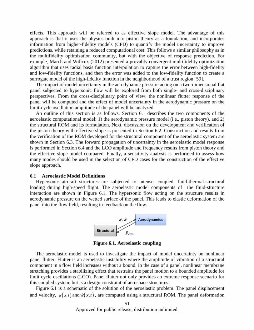
effects. This approach will be referred to as effective slope model. The advantage of this approach is that it uses the physics built into piston theory as a foundation, and incorporates information from higher-fidelity models (CFD) to quantify the model uncertainty to improve predictions, while retaining a reduced computational cost. This follows a similar philosophy as in the multifidelity optimization community, but with the objective of response prediction. For example, March and Willcox (2012) presented a provably convergent multifidelity optimization algorithm that uses radial basis function interpolation to capture the error between high-fidelity and low-fidelity functions, and then the error was added to the low-fidelity function to create a surrogate model of the high-fidelity function in the neighborhood of a trust region [59].
The impact of model uncertainty in the aerodynamic pressure acting on a two-dimensional flat panel subjected to hypersonic flow will be explored from both single- and cross-disciplinary perspectives. From the cross-disciplinary point of view, the nonlinear flutter response of the panel will be computed and the effect of model uncertainty in the aerodynamic pressure on the limit-cycle oscillation amplitude of the panel will be analyzed.
An outline of this section is as follows. Section 6.1 describes the two components of the aeroelastic computational model: 1) the aerodynamic pressure model (i.e., piston theory), and 2) the structural ROM and its formulation. Next, discussion on the development and verification of the piston theory with effective slope is presented in Section 6.2. Construction and results from the verification of the ROM developed for the structural component of the aeroelastic system are shown in Section 6.3. The forward propagation of uncertainty in the aeroelastic model response is performed in Section 6.4 and the LCO amplitude and frequency results from piston theory and the effective slope model compared. Finally, a sensitivity analysis is performed to assess how many modes should be used in the selection of CFD cases for the construction of the effective slope approach.
6.1 Aeroelastic Model Definitions Hypersonic aircraft structures are subjected to intense, coupled, fluid-thermal-structural
loading during high-speed flight. The aeroelastic model components of the fluid-structure interaction are shown in Figure 6.1. The hypersonic flow acting on the structure results in aerodynamic pressure on the wetted surface of the panel. This leads to elastic deformation of the panel into the flow field, resulting in feedback on the flow.
Figure 6.1. Aeroelastic coupling
The aeroelastic model is used to investigate the impact of model uncertainty on nonlinear panel flutter. Flutter is an aeroelastic instability where the amplitude of vibration of a structural component in a flow field increases without a bound. In the case of a panel, nonlinear membrane stretching provides a stabilizing effect that restrains the panel motion to a bounded amplitude for limit cycle oscillations (LCO). Panel flutter not only provides an extreme response scenario for this coupled system, but is a design constraint of aerospace structures.
Figure 6.1 is a schematic of the solution of the aeroelastic problem. The panel displacement and velocity, ( ),w x t and ( ),w x t , are computed using a structural ROM. The panel deformation
Structural
Aerodynamicsww ,
aerop
51 Approved for public release; distribution unlimited.
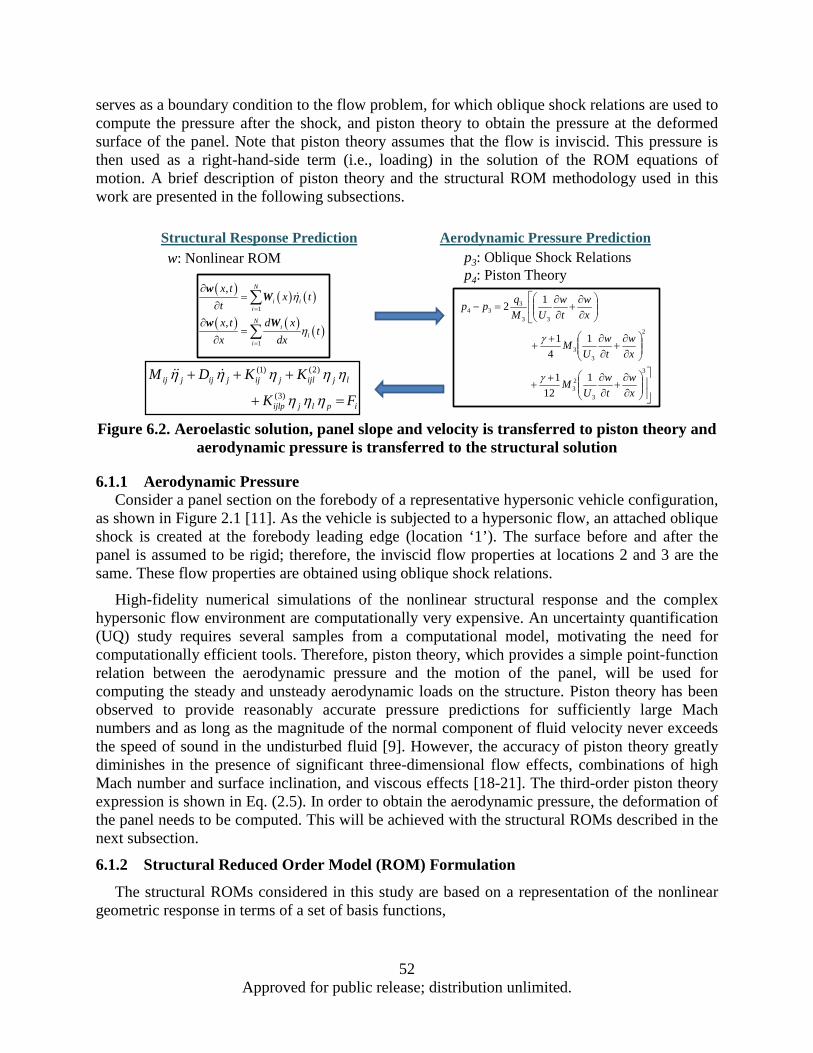
serves as a boundary condition to the flow problem, for which oblique shock relations are used to compute the pressure after the shock, and piston theory to obtain the pressure at the deformed surface of the panel. Note that piston theory assumes that the flow is inviscid. This pressure is then used as a right-hand-side term (i.e., loading) in the solution of the ROM equations of motion. A brief description of piston theory and the structural ROM methodology used in this work are presented in the following subsections.
Figure 6.2. Aeroelastic solution, panel slope and velocity is transferred to piston theory and
aerodynamic pressure is transferred to the structural solution
6.1.1 Aerodynamic Pressure Consider a panel section on the forebody of a representative hypersonic vehicle configuration,
as shown in Figure 2.1 [11]. As the vehicle is subjected to a hypersonic flow, an attached oblique shock is created at the forebody leading edge (location ‘1’). The surface before and after the panel is assumed to be rigid; therefore, the inviscid flow properties at locations 2 and 3 are the same. These flow properties are obtained using oblique shock relations.
High-fidelity numerical simulations of the nonlinear structural response and the complex hypersonic flow environment are computationally very expensive. An uncertainty quantification (UQ) study requires several samples from a computational model, motivating the need for computationally efficient tools. Therefore, piston theory, which provides a simple point-function relation between the aerodynamic pressure and the motion of the panel, will be used for computing the steady and unsteady aerodynamic loads on the structure. Piston theory has been observed to provide reasonably accurate pressure predictions for sufficiently large Mach numbers and as long as the magnitude of the normal component of fluid velocity never exceeds the speed of sound in the undisturbed fluid [9]. However, the accuracy of piston theory greatly diminishes in the presence of significant three-dimensional flow effects, combinations of high Mach number and surface inclination, and viscous effects [18-21]. The third-order piston theory expression is shown in Eq. (2.5). In order to obtain the aerodynamic pressure, the deformation of the panel needs to be computed. This will be achieved with the structural ROMs described in the next subsection.
6.1.2 Structural Reduced Order Model (ROM) Formulation
The structural ROMs considered in this study are based on a representation of the nonlinear geometric response in terms of a set of basis functions,
∂∂
+∂∂+
+
∂∂
+∂∂+
+
∂∂
+∂∂
=−
3
3
23
2
33
33
334
112
1
14
1
12
xw
tw
UM
xw
tw
UM
xw
tw
UMqpp
γ
γ
( ) ( ) ( )
( ) ( ) ( )
1
1
,
,
N
i ii
Ni
ii
x tx t
tx t d x
tx dx
η
η
=
=
∂=
∂∂
=∂
∑
∑
w
W
w W
ipljijlp
ljijljijjijjij
FK
KKDM
=+
+++
ηηη
ηηηηη)3(
)2()1(
Structural Response Prediction Aerodynamic Pressure Predictionw: Nonlinear ROM p3: Oblique Shock Relations
p4: Piston Theory
52 Approved for public release; distribution unlimited.
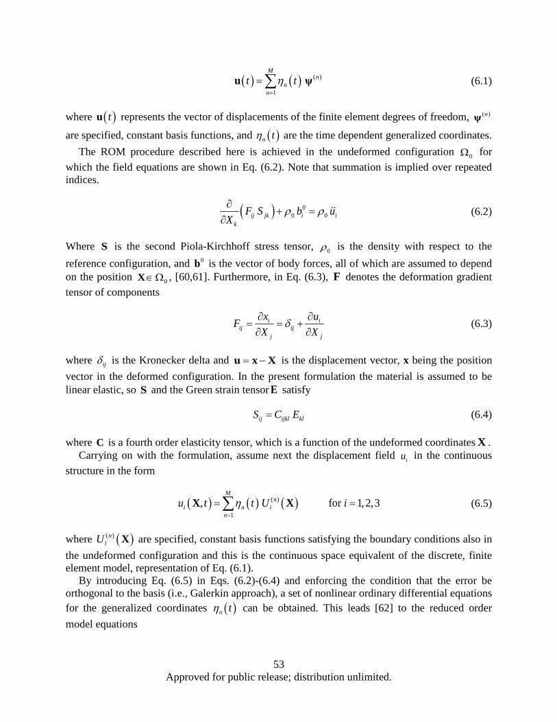
( ) ( ) ( )
1
Mn
nn
t tη=
= ∑u ψ (6.1)
where ( )tu represents the vector of displacements of the finite element degrees of freedom, ( )nψ
are specified, constant basis functions, and ( )n tη are the time dependent generalized coordinates. The ROM procedure described here is achieved in the undeformed configuration 0Ω for
which the field equations are shown in Eq. (6.2). Note that summation is implied over repeated indices.
( ) 00 0ij jk i i
k
F S b uX
ρ ρ∂+ =
∂ (6.2)
Where S is the second Piola-Kirchhoff stress tensor, 0ρ is the density with respect to the reference configuration, and 0b is the vector of body forces, all of which are assumed to depend on the position 0∈ΩX , [60,61]. Furthermore, in Eq. (6.3), F denotes the deformation gradient tensor of components
i iij ij
j j
x uFX X
δ∂ ∂= = +
∂ ∂ (6.3)
where ijδ is the Kronecker delta and = −u x X is the displacement vector, x being the position vector in the deformed configuration. In the present formulation the material is assumed to be linear elastic, so S and the Green strain tensor E satisfy
ij ijkl klS C E= (6.4)
where C is a fourth order elasticity tensor, which is a function of the undeformed coordinates X . Carrying on with the formulation, assume next the displacement field iu in the continuous
structure in the form
( ) ( ) ( )( )
1, for 1, 2,3
Mn
i n in
u t t U iη=
= =∑X X (6.5)
where ( )( )niU X are specified, constant basis functions satisfying the boundary conditions also in
the undeformed configuration and this is the continuous space equivalent of the discrete, finite element model, representation of Eq. (6.1).
By introducing Eq. (6.5) in Eqs. (6.2)-(6.4) and enforcing the condition that the error be orthogonal to the basis (i.e., Galerkin approach), a set of nonlinear ordinary differential equations for the generalized coordinates ( )n tη can be obtained. This leads [62] to the reduced order model equations
53 Approved for public release; distribution unlimited.

(1) (2) (3)ij j ij j ij j ijl j l ijlp j l p iM D K K K Fη η η η η η η η+ + + + = (6.6)
where a linear damping term ij jD η has been added to collectively represent various dissipation
mechanisms. Furthermore, ijM denotes the elements of the mass matrix, (1)ijK , (2)
ijlK , (3)ijlpK are
the linear, quadratic, and cubic stiffness coefficients and iF are the modal forces. The indirect evaluation of the coefficients in Eq. (6.6) by Hollkamp and Gordon (2005) from a finite element model is used here [63].
With the aerodynamic pressure and structural response models defined, the next section will investigate and quantify the model-form uncertainty in the aerodynamic pressure predictions obtained with piston theory.
6.2 Model Uncertainty in Aerodynamic Pressure The objective of mathematical models is to make predictions about the behavior of a system.
However, no model is perfect due to various sources of uncertainty, so the predictions will not exactly equal the true value of the process it is intended to represent. Model uncertainty (also referred to as model inadequacy) can be defined as the difference between the true mean of the process and the output of the model at specified inputs [21]. Model uncertainty δ can be introduced in two general forms. First, by adding a non-intrusive, external model discrepancy term, as shown in Eq. (6.7).
( ),y m x φ δ ε= + + (6.7)
Where x are the model inputs, φ are the uncertain model parameters, and ε represents the measurement uncertainty. A separate model discrepancy term is a commonly-used and flexible approach to quantifying the model form uncertainty in m [21,45]. However, it may be desirable to capture the nature of the model inadequacy at the source of the error within the model itself, as shown in Eq. (6.8) [58]. This can help preserve the underlying physics and original model form, while still providing an improved, uncertainty-quantified prediction.
( ), ,y m x φ δ ε= + (6.8)
The external and internal model discrepancy approaches are discussed in the following subsections in the context of model uncertainty in aerodynamic pressure predictions using piston theory.
6.2.1 External Discrepancy Model Under realistic flow conditions, model-form error exists in piston theory due to unmodeled
flow viscosity and significant three-dimensionality of the flow [55-57]. Using data available from tests conducted by Glass and Hunt (1986) on spherical dome protuberances subjected to hypersonic flow [44], Culler and McNamara (2010) [10] showed peak and average pressure discrepancies in piston theory of 54.5% and 18.6%, respectively. In a different study, DeCarlo et al. (2013) identified and calibrated through a Bayesian network a model-form error function with respect to the slope of the surface for selected domes from the Glass and Hunt tests [24]. The form of the model (i.e., quadratic polynomial) was inferred from an initial interrogation of the
54 Approved for public release; distribution unlimited.
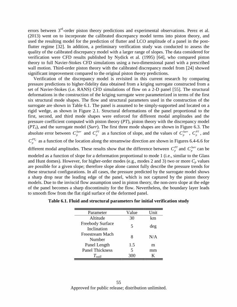
errors between 3rd-order piston theory predictions and experimental observations. Perez et al. (2013) went on to incorporate the calibrated discrepancy model terms into piston theory, and used the resulting model for the prediction of flutter and LCO amplitude of a panel in the post-flutter regime [32]. In addition, a preliminary verification study was conducted to assess the quality of the calibrated discrepancy model with a larger range of slopes. The data considered for verification were CFD results published by Nydick et al. (1995) [64], who compared piston theory to full Navier-Stokes CFD simulations using a two-dimensional panel with a prescribed wall motion. Third-order piston theory with the calibrated discrepancy model from [24] showed significant improvement compared to the original piston theory predictions.
Verification of the discrepancy model is revisited in this current research by comparing pressure predictions to higher-fidelity data obtained from a kriging surrogate constructed from a set of Navier-Stokes (i.e. RANS) CFD simulations of flow on a 2-D panel [55]. The structural deformations in the construction of the kriging surrogate were parameterized in terms of the first six structural mode shapes. The flow and structural parameters used in the construction of the surrogate are shown in Table 6.1. The panel is assumed to be simply-supported and located on a rigid wedge, as shown in Figure 2.1. Structural deformations of the panel proportional to the first, second, and third mode shapes were enforced for different modal amplitudes and the pressure coefficient computed with piston theory (PT), piston theory with the discrepancy model (PTδ), and the surrogate model (Surr). The first three mode shapes are shown in Figure 6.3. The absolute error between Surr
pC and PTpC as a function of slope, and the values of Surr
pC , PTpC , and
PTpC δ as a function of the location along the streamwise direction are shown in Figures 6.4-6.6 for
different modal amplitudes. These results show that the difference between PTpC and Surr
pC can be modeled as a function of slope for a deformation proportional to mode 1 (i.e., similar to the Glass and Hunt domes). However, for higher-order modes (e.g., modes 2 and 3) two or more Cp values are possible for a given slope; therefore slope alone cannot fully describe the pressure trends for these structural configurations. In all cases, the pressure predicted by the surrogate model shows a sharp drop near the leading edge of the panel, which is not captured by the piston theory models. Due to the inviscid flow assumption used in piston theory, the non-zero slope at the edge of the panel becomes a sharp discontinuity for the flow. Nevertheless, the boundary layer leads to smooth flow from the flat rigid surface of the deformed panel.
Table 6.1. Fluid and structural parameters for initial verification study
Parameter Value Unit Altitude 30 km
Freebody Surface Inclination 5 deg
Freestream Mach Number 8 N/A
Panel Length 1.5 m Panel Thickness 5 mm
Twall 300 K
55 Approved for public release; distribution unlimited.
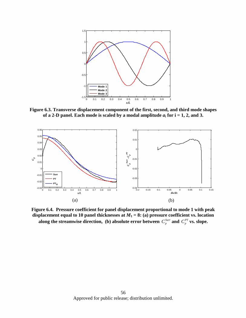
Figure 6.3. Transverse displacement component of the first, second, and third mode shapes
of a 2-D panel. Each mode is scaled by a modal amplitude ai for i = 1, 2, and 3.
(a)
(b)
Figure 6.4. Pressure coefficient for panel displacement proportional to mode 1 with peak displacement equal to 10 panel thicknesses at M1 = 8: (a) pressure coefficient vs. location
along the streamwise direction, (b) absolute error between SurrpC and PT
pC vs. slope.
0 0.1 0.2 0.3 0.4 0.5 0.6 0.7 0.8 0.9 1-1.5
-1
-0.5
0
0.5
1
1.5
x/L
Mode 1Mode 2Mode 3
0 0.1 0.2 0.3 0.4 0.5 0.6 0.7 0.8 0.9 1-0.03
-0.02
-0.01
0
0.01
0.02
0.03
0.04
0.05
0.06
x/L
CP
Surr
PT
PTdeltaδ
-0.2 -0.15 -0.1 -0.05 0 0.05 0.1 0.15-0.04
-0.03
-0.02
-0.01
0
0.01
0.02
dw/dx
CpSu
rr -
CpPT
56 Approved for public release; distribution unlimited.
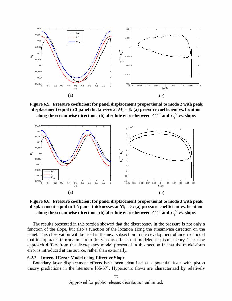
(a)
(b)
Figure 6.5. Pressure coefficient for panel displacement proportional to mode 2 with peak displacement equal to 3 panel thicknesses at M1 = 8: (a) pressure coefficient vs. location
along the streamwise direction, (b) absolute error between SurrpC and PT
pC vs. slope.
(a)
(b)
Figure 6.6. Pressure coefficient for panel displacement proportional to mode 3 with peak displacement equal to 1.5 panel thicknesses at M1 = 8: (a) pressure coefficient vs. location
along the streamwise direction, (b) absolute error between SurrpC and PT
pC vs. slope.
The results presented in this section showed that the discrepancy in the pressure is not only a function of the slope, but also a function of the location along the streamwise direction on the panel. This observation will be used in the next subsection in the development of an error model that incorporates information from the viscous effects not modeled in piston theory. This new approach differs from the discrepancy model presented in this section in that the model-form error is introduced at the source, rather than externally.
6.2.2 Internal Error Model using Effective Slope Boundary layer displacement effects have been identified as a potential issue with piston
theory predictions in the literature [55-57]. Hypersonic flows are characterized by relatively
0 0.1 0.2 0.3 0.4 0.5 0.6 0.7 0.8 0.9 1-0.015
-0.01
-0.005
0
0.005
0.01
0.015
0.02
0.025
0.03
x/L
CP
Surr
PT
PTdeltaδ
-0.08 -0.06 -0.04 -0.02 0 0.02 0.04 0.06 0.08-0.02
-0.015
-0.01
-0.005
0
0.005
0.01
dw/dx
CpSu
rr -
CpPT
0 0.1 0.2 0.3 0.4 0.5 0.6 0.7 0.8 0.9 1-0.025
-0.02
-0.015
-0.01
-0.005
0
0.005
0.01
0.015
0.02
0.025
x/L
CP
SurrPTPTdeltaδ
-0.05 -0.04 -0.03 -0.02 -0.01 0 0.01 0.02 0.03 0.04 0.05-12
-10
-8
-6
-4
-2
0
2
4
6
8x 10
-3
dw/dx
CpSu
rr -
CpPT
57 Approved for public release; distribution unlimited.
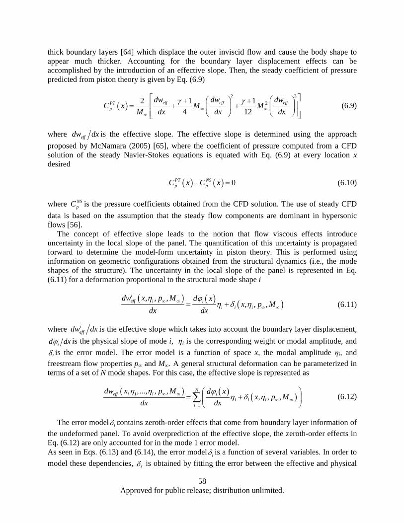
thick boundary layers [64] which displace the outer inviscid flow and cause the body shape to appear much thicker. Accounting for the boundary layer displacement effects can be accomplished by the introduction of an effective slope. Then, the steady coefficient of pressure predicted from piston theory is given by Eq. (6.9)
( )2 3
22 1 14 12
eff eff effPTp
dw dw dwC x M M
M dx dx dxγ γ
∞ ∞∞
+ += + +
(6.9)
where effdw dx is the effective slope. The effective slope is determined using the approach proposed by McNamara (2005) [65], where the coefficient of pressure computed from a CFD solution of the steady Navier-Stokes equations is equated with Eq. (6.9) at every location x desired
( ) ( ) 0PT NSp pC x C x− = (6.10)
where NSpC is the pressure coefficients obtained from the CFD solution. The use of steady CFD
data is based on the assumption that the steady flow components are dominant in hypersonic flows [56].
The concept of effective slope leads to the notion that flow viscous effects introduce uncertainty in the local slope of the panel. The quantification of this uncertainty is propagated forward to determine the model-form uncertainty in piston theory. This is performed using information on geometric configurations obtained from the structural dynamics (i.e., the mode shapes of the structure). The uncertainty in the local slope of the panel is represented in Eq. (6.11) for a deformation proportional to the structural mode shape i
( ) ( ) ( )
, , ,, , ,
ieff i i
i i i
dw x p M d xx p M
dx dxη ϕ
η δ η∞ ∞∞ ∞= + (6.11)
where ieffdw dx is the effective slope which takes into account the boundary layer displacement,
id dxϕ is the physical slope of mode i, ηi is the corresponding weight or modal amplitude, and
iδ is the error model. The error model is a function of space x, the modal amplitude ηi, and freestream flow properties p∞ and M∞. A general structural deformation can be parameterized in terms of a set of N mode shapes. For this case, the effective slope is represented as
( ) ( ) ( )1
1
, ,..., , ,, , ,
Neff i i
i i ii
dw x p M d xx p M
dx dxη η ϕ
η δ η∞ ∞∞ ∞
=
= +
∑ (6.12)
The error model iδ contains zeroth-order effects that come from boundary layer information of the undeformed panel. To avoid overprediction of the effective slope, the zeroth-order effects in Eq. (6.12) are only accounted for in the mode 1 error model. As seen in Eqs. (6.13) and (6.14), the error model iδ is a function of several variables. In order to model these dependencies, iδ is obtained by fitting the error between the effective and physical
58 Approved for public release; distribution unlimited.
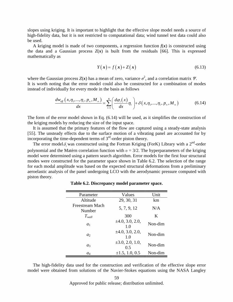
slopes using kriging. It is important to highlight that the effective slope model needs a source of high-fidelity data, but it is not restricted to computational data; wind tunnel test data could also be used.
A kriging model is made of two components, a regression function f(x) is constructed using the data and a Gaussian process Z(x) is built from the residuals [66]. This is expressed mathematically as
( ) ( ) ( )Y f Z= +x x x (6.13)
where the Gaussian process Z(x) has a mean of zero, variance σ2, and a correlation matrix Ψ. It is worth noting that the error model could also be constructed for a combination of modes instead of individually for every mode in the basis as follows
( ) ( ) ( )11
1
, ,..., , ,, ,..., , ,
Neff i i
i ii
dw x p M d xx p M
dx dxη η ϕ
η δ η η∞ ∞∞ ∞
=
= +
∑ (6.14)
The form of the error model shown in Eq. (6.14) will be used, as it simplifies the construction of the kriging models by reducing the size of the input space.
It is assumed that the primary features of the flow are captured using a steady-state analysis [55]. The unsteady effects due to the surface motion of a vibrating panel are accounted for by incorporating the time-dependent terms of 3rd-order piston theory.
The error model iδ was constructed using the Fortran Kriging (ForK) Library with a 2nd-order polynomial and the Matèrn correlation function with υ = 3/2. The hyperparameters of the kriging model were determined using a pattern search algorithm. Error models for the first four structural modes were constructed for the parameter space shown in Table 6.2. The selection of the range for each modal amplitude was based on the expected structural deformations from a preliminary aeroelastic analysis of the panel undergoing LCO with the aerodynamic pressure computed with piston theory.
Table 6.2. Discrepancy model parameter space.
Parameter Values Unit Altitude 29, 30, 31 km
Freestream Mach Number 5, 7, 9, 12 N/A
Twall 300 K
a1 ±4.0, 3.0, 2.0,
1.0 Non-dim
a2 ±4.0, 3.0, 2.0,
1.0 Non-dim
a3 ±3.0, 2.0, 1.0,
0.5 Non-dim
a4 ±1.5, 1.0, 0.5 Non-dim The high-fidelity data used for the construction and verification of the effective slope error
model were obtained from solutions of the Navier-Stokes equations using the NASA Langley
59 Approved for public release; distribution unlimited.
CFL3D code. This code uses an implicit, finite-volume algorithm based on upwind-biased spatial differencing to solve the Reynolds Averaged Navier-Stokes (RANS) equations. No real gas effects were included in the analysis since CFL3D is an ideal gas code. The Menter κ–ω SST turbulence model is used here for closure of the RANS equations [39]. The computational mesh used in this study is the one built by Crowell et al. (2011) with a total of 34,600 cells with a maximum y+ value at the wall of 0.65 [55]. Also, the upstream surface was modeled such that the transition to turbulent flow occurs one meter upstream of the leading edge of the panel. A clamped-clamped 2-D panel is considered in this study as these boundary conditions are more representative of what is found in real aircraft structures.
The first four mode shapes of the 2-D clamped-clamped panel are shown in Figure 6.7; note that the zero slope at the leading and trailing edges of the panel eliminate the discontinuity seen by the flow that was discussed for the simply-supported panel. Shown in Figure 6.8 is the pressure coefficient along the length of the panel for rigid panel shape obtained from the combination of the first four structural modes with the following modal amplitudes: a1 = +3, a2 = -3.25, a3 = +1.25, and a4 = -0.15. The results were obtained at a freestream Mach number of M1 = 10 and an altitude of 30km, and computed with CFD (NS), piston theory (PT) and piston theory with effective slope (PTeff). The PTeff results show a close agreement with the NS data. Based on the L∞ error metric, the error between effPT
pC and NSpC is of 4.7% versus 30% between
PTpC and NS
pC . The remaining model uncertainty in the effPTpC prediction is likely to come from
the limitations of kriging and the use of a finite number of training data. The verification under unsteady conditions was performed by enforcing the panel motion as
follows
( ) ( ) ( ), sini iw x t a t xw ϕ= (6.15)
where ai is the amplitude of mode φi(x) and ω is the frequency of vibration in rad/sec. Shown in Figures 6.8-6.12 are the Generalized Aerodynamic Forces (GAFs) obtained from CFD
( ( )NSGAF ), piston theory ( ( )PTGAF ), and piston theory with effective slope ( ( )effPTGAF ). From Eq. (6.16), L and c are the length and width of the panel for displacements proportional to modes 1, 2, 3, and 4, an oscillation frequency of 100Hz, and the same freestream flow properties considered in the verification of the steady-state analysis. The modal amplitudes of the panel motion used were a1 = +3.0, a2 = +2.0, a3 = +1.0, and a4 = +0.5. Table 6.3 shows results that
quantitatively compare ( )NSGAF to ( )PTGAF and ( )effPTGAF . With maximum errors
approximately an order of magnitude less than ( )PTGAF , the ( )effPTGAF results show closer agreement with ( )NSGAF .
Recall that the intent of this research is to identify missing physics within computational models, and develop an internal error model to quantify the model-form uncertainty. A kriging surrogate was selected to model the internal error through effective slope. This is in contrast to external, non-intrusive approaches, as those represented by Eq. (6.8), where the model-form uncertainty is quantified directly by comparing the model predictions against experimental observations. In the case of the PT model, viscous effects in the form of boundary layer displacement thickness were identified as important information that is not included in the model. The objective of the PTeff model was to incorporate this missing information in PT. The
60 Approved for public release; distribution unlimited.

quantification of model-form uncertainty with the PTeff model corroborates the importance of viscous effects in hypersonic flows.
( ) ( ) ( )0
,L
i i AGAF t c x p x t dxϕ= ∫ for i = 1,..., N. (6.16)
Table 6.3. Difference in GAFs for the Navier-Stokes solution compared to piston theory and piston theory with the effective slope model.
Method
Max Diff. GAFs
Mode 1 (%)
Max Diff. GAFs
Mode 2 (%)
Max Diff. GAFs
Mode 3 (%)
Max Diff. GAFs
Mode 4 (%)
( )PTGAF 120 100.3 107.6 100.2 ( )effPTGAF 10.6 9.2 8.6 7.6
Figure 6.7. Transverse displacement component of the first, second, third, and fourth mode shapes of a 2-D clamped-clamped panel. Each mode is scaled by a modal amplitude ai for
i=1, 2, 3, and 4
0 0.1 0.2 0.3 0.4 0.5 0.6 0.7 0.8 0.9 1-1
-0.8
-0.6
-0.4
-0.2
0
0.2
0.4
0.6
0.8
1
x/L
Mode 1Mode 2Mode 3Mode 4
61 Approved for public release; distribution unlimited.
Figure 6.8. Navier-Stokes, piston theory, and piston theory with effective slope model
pressure coefficient for panel displacement proportional to a combination of modes 1, 2, 3, and 4 at M1 = 10, with modal amplitudes a1 = +3.0, a2 = -3.25, a3 = +1.25, a4 = -0.15
Figure 6.9. Navier-Stokes, piston theory, and piston theory with effective slope Generalized Aerodynamic Forces for enforced panel motion w(x,t) = a1 sin(ωt)φ(x) proportional to mode
1 and frequency equal to 100Hz at M1 = 10
0 0.1 0.2 0.3 0.4 0.5 0.6 0.7 0.8 0.9 1-0.02
-0.01
0
0.01
0.02
0.03
0.04
x/L
CP
NSPTPTeff
0 0.5 1 1.5 2 2.5-400
-300
-200
-100
0
100
200
300
400
Non-Dimensional Time (Cycles)
GA
F (N
)
GAF(NS)
GAF(PT)
GAF(PTeff
)
62 Approved for public release; distribution unlimited.
Figure 6.10. Navier-Stokes, piston theory, and piston theory with effective slope
Generalized Aerodynamic Forces for enforced panel motion w(x,t) = a2 sin(ωt)φ(x) proportional to mode 2 and frequency equal to 100Hz at M1 = 10
Figure 6.11. Navier-Stokes, piston theory, and piston theory with effective slope
Generalized Aerodynamic Forces for enforced panel motion w(x,t) = a3 sin(ωt)φ(x) proportional to mode 3 and frequency equal to 100Hz at M1 = 10
0 0.5 1 1.5 2 2.5
-400
-200
0
200
400
600
Non-Dimensional Time (Cycles)
GA
F (N
)
GAF(NS)
GAF(PT)
GAF(PTeff
)
0 0.5 1 1.5 2 2.5-300
-200
-100
0
100
200
300
400
500
Non-Dimensional Time (Cycles)
GA
F (N
)
GAF(NS)
GAF(PT)
GAF(PTeff
)
63 Approved for public release; distribution unlimited.
Figure 6.12. Navier-Stokes, piston theory, and piston theory with effective slope
Generalized Aerodynamic Forces for enforced panel motion w(x,t) = a4 sin(ωt)φ(x) proportional to mode 4 and frequency equal to 100Hz at M1 = 10
The uncertainty quantified in this model will be propagated to the aeroelastic quantity of interest (i.e., limit cycle oscillations) in Section 6.4. However, the next step is to generate and verify the other component to the coupled aeroelastic model, namely the structural ROM.
6.3 Structural Reduced-Order Model (ROM) Construction and Verification A structural ROM introduces uncertainty in the analysis in the form of solution approximation
errors, which is related to the number of basis functions used to construct the ROM. As described in Section 6.1, the structural ROMs used in this study are built from a finite element analysis (FEA) model; therefore, its predictions can only be as good as the predictions from the FEA model that was used to construct it.
A ROM built with 6 linear modes was constructed for an isotropic 2-D panel clamped along the sides perpendicular to the direction of the flow. The geometric, material properties of the panel, and flow conditions are shown in Table 6.4. The ROM was constructed with an in-house FEA beam model based on a co-rotational formulation capable of analyzing problems with large rotations and small strains. The FEA model was built using 40 beam elements, a total of 123 degrees-of-freedom. A mesh convergence analysis was performed with respect to the first six natural frequencies of the panel and the nonlinear stiffness coefficient K1111.
Table 6.4. Aeroelastic model parameters
Parameter Value Unit Altitude 30 km
Freebody Surface Inclination 5 deg Freestream Mach Number 5-12 N/A
Panel Length 1.5 m Panel Thickness 2 mm
Modulus of Elasticity 113 GPa Density 4539 kg/m3
0 0.5 1 1.5 2 2.5-200
-150
-100
-50
0
50
100
150
200
250
300
Non-Dimensional Time (Cycles)
GA
F (N
)
GAF(NS)
GAF(PT)
GAF(PTeff
)
64 Approved for public release; distribution unlimited.

The ROM and the FEA model were coupled with PT to predict the aeroelastic response of the panel. The quantities of interest are: the LCO amplitude and frequency. These quantities are critical for aircraft structural design, since they drive the fatigue life of the panel. The LCO amplitude is the maximum displacement for every period of oscillation and it occurs at the ¾-point along the length of the panel.
Shown in Figure 6.13 is a comparison of the LCO amplitude as a function of the Mach number. The maximum error of the 6-mode ROM relative to the FEA results occurs at a Mach number of 12 and is equal to approximately 2%. Shown in Figure 15 is the LCO frequency as a function of the Mach number. The maximum relative error in the LCO frequency between the 6-mode ROM and the FEA is equal to 10% which corresponds to a difference of approximately 2Hz. As the LCO amplitude grows, oscillations about the deformed configuration become stiffer, this is seen by the increasing LCO frequency with respect to the Mach number. The quantification of the solution approximation error introduced by the 6-mode ROM suggests that more modes would be needed for Mach numbers larger than 12.
Figure 6.13. LCO amplitude at panel three-quarter point as a function of Mach number
for air properties calculated at an altitude of 30km, FEA, 6-Mode ROM, and 4-Mode ROM coupled with 3rd-order piston theory
5 6 7 8 9 10 11 120
0.5
1
1.5
2
2.5
Mach Number
LCO
Am
plitu
de (P
anel
Thi
ckne
sses
)
FEA6-Mode ROM
65 Approved for public release; distribution unlimited.
Figure 6.14. LCO frequency as a function of Mach number for air properties calculated at an altitude of 30km, FEA, 6-Mode ROM, and 4-Mode ROM coupled with 3rd-order piston
theory
The next section investigates the effect of model-form uncertainty in aerodynamic pressure predictions on the LCO amplitude and frequency of a panel.
6.4 Uncertainty Propagation to Coupled Aeroelastic Model Response The internal error from Section 6.2 captured the effect of model-form uncertainty through the
effective slope used in aerodynamic pressure predictions from piston theory. The PTeff model is used here to investigate the effect of model-form uncertainty from aereodynamic pressure predictions on the coupled aeroelastic response of the 2-D panel described in the previous section. The structural solution was obtained using the 6-mode ROM; however, the PTeff model only contains information from the first four dominant modes, as the modal amplitudes of the last two modes are relatively smaller. The validity of this assumption will be investigated through the sensitivity analysis of the four modes at the end of this section. Variability in the inputs was modeled with statistical distributions for the freestream pressure p1 and the modulus of elasticity E. Normal distributions were used with means equal to their nominal values shown in Table 6.4 and 1% coefficients of variation. Prior knowledge on the model-form uncertainty in PT predictions was incorporated based on previous reports [9] which indicated that PT predictions are expected to be accurate within [-19%, 0%]. Figures 6.15 and 6.16 show the mean and 95% confidence bounds of the LCO amplitude and frequency as a function of the freestream Mach number from 1,000 Monte Carlo samples. The effects of model-form uncertainty in aerodynamic pressure, quantified with the PTeff model, become more pronounced for increasing Mach numbers. At a Mach number of 12, the mean values of the LCO amplitude and frequency are 44% and 13% lower, respectively, when model-form uncertainty from viscous effects in the aerodynamic pressure prediction is incorporated. Increasing discrepancies in the LCO amplitude and frequency imply larger uncertainty in the stress amplitude and number of cycles that the structure is subjected to. Therefore, future work will consider the analysis of the impact of model uncertianty on the fatigue life of the panel.
6 7 8 9 10 11 1210
12
14
16
18
20
22
24
26
Mach Number
LCO
Fre
quen
cy (H
z)
FEA6-Mode ROM
66 Approved for public release; distribution unlimited.
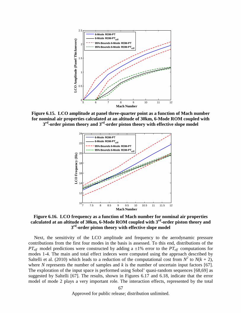
Figure 6.15. LCO amplitude at panel three-quarter point as a function of Mach number for nominal air properties calculated at an altitude of 30km, 6-Mode ROM coupled with
3rd-order piston theory and 3rd-order piston theory with effective slope model
Figure 6.16. LCO frequency as a function of Mach number for nominal air properties
calculated at an altitude of 30km, 6-Mode ROM coupled with 3rd-order piston theory and 3rd-order piston theory with effective slope model
Next, the sensitivity of the LCO amplitude and frequency to the aerodynamic pressure contributions from the first four modes in the basis is assessed. To this end, distributions of the PTeff model predictions were constructed by adding a ±1% error to the PTeff computations for modes 1-4. The main and total effect indeces were computed using the approach described by Saltelli et al. (2010) which leads to a reduction of the computational cost from N2 to N(k + 2), where N represents the number of samples and k is the number of uncertain input factors [67]. The exploration of the input space is performed using Sobol’ quasi-random sequences [68,69] as suggested by Saltelli [67]. The results, shown in Figures 6.17 and 6.18, indicate that the error model of mode 2 plays a very important role. The interaction effects, represented by the total
5 6 7 8 9 10 11 120
0.5
1
1.5
2
2.5
Mach Number
LCO
Am
plitu
de (P
anel
Thi
ckne
sses
)
6-Mode ROM-PT6-Mode ROM-PTeff95% Bounds 6-Mode ROM-PT95% Bounds 6-Mode ROM-PTeff
7 7.5 8 8.5 9 9.5 10 10.5 11 11.5 1210
12
14
16
18
20
22
24
Mach Number
LCO
Fre
quen
cy (H
z)
6-Mode ROM-PT6-Mode ROM-PTeff95% Bounds 6-Mode ROM-PT95% Bounds 6-Mode ROM-PTeff
67 Approved for public release; distribution unlimited.

effect index, are stronger than the first-order effects for modes 1, 3, and 4. These results suggest that the error models of the asymmetric modes (i.e. modes 2 and 4) play a more important role than the symmetric modes (i.e. modes 1 and 3). This is not surprising based on the discussion from Section 6.2 which indicated that the model-form error becomes more complex for increasing mode numbers. These results also imply that the PTeff model should contain information from mode 6 (i.e. the next asymmetric mode) as well. These conclusions indicate that the information from a sensitivity analysis can be used to guide the construction of the PTeff model.
Figure 6.17. First-order effect sensitivity indices for remaining model-form uncertainty in
effective slope model as a function of Mach number, modes 1 to 4
Figure 6.18. Total effect sensitivity indices for remaining model-form uncertainty in
effective slope model as a function of Mach number, modes 1 to 4
8 8.5 9 9.5 10 10.5 11 11.5 120
0.1
0.2
0.3
0.4
0.5
0.6
0.7
Mach Number
S i
Mode 1Mode 2Mode 3Mode 4
8 8.5 9 9.5 10 10.5 11 11.5 120
0.1
0.2
0.3
0.4
0.5
0.6
Mach Number
S T i
Mode 1Mode 2Mode 3Mode 4
68 Approved for public release; distribution unlimited.
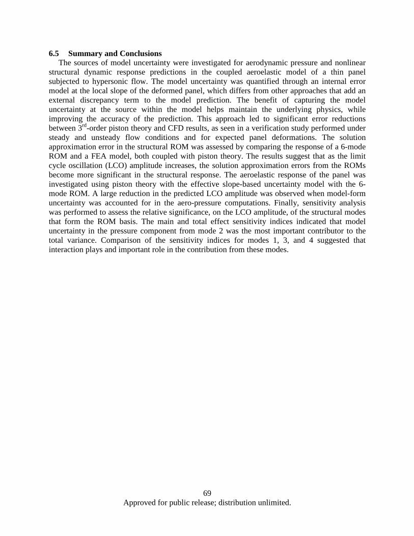
6.5 Summary and Conclusions The sources of model uncertainty were investigated for aerodynamic pressure and nonlinear
structural dynamic response predictions in the coupled aeroelastic model of a thin panel subjected to hypersonic flow. The model uncertainty was quantified through an internal error model at the local slope of the deformed panel, which differs from other approaches that add an external discrepancy term to the model prediction. The benefit of capturing the model uncertainty at the source within the model helps maintain the underlying physics, while improving the accuracy of the prediction. This approach led to significant error reductions between 3rd-order piston theory and CFD results, as seen in a verification study performed under steady and unsteady flow conditions and for expected panel deformations. The solution approximation error in the structural ROM was assessed by comparing the response of a 6-mode ROM and a FEA model, both coupled with piston theory. The results suggest that as the limit cycle oscillation (LCO) amplitude increases, the solution approximation errors from the ROMs become more significant in the structural response. The aeroelastic response of the panel was investigated using piston theory with the effective slope-based uncertainty model with the 6-mode ROM. A large reduction in the predicted LCO amplitude was observed when model-form uncertainty was accounted for in the aero-pressure computations. Finally, sensitivity analysis was performed to assess the relative significance, on the LCO amplitude, of the structural modes that form the ROM basis. The main and total effect sensitivity indices indicated that model uncertainty in the pressure component from mode 2 was the most important contributor to the total variance. Comparison of the sensitivity indices for modes 1, 3, and 4 suggested that interaction plays and important role in the contribution from these modes.
69 Approved for public release; distribution unlimited.
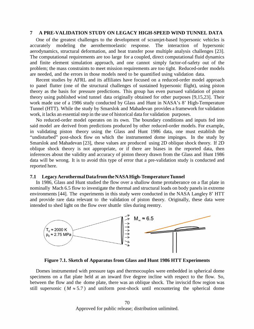
7 A PRE-VALIDATION STUDY ON LEGACY HIGH-SPEED WIND TUNNEL DATA One of the greatest challenges to the development of scramjet-based hypersonic vehicles is
accurately modeling the aerothermoelastic response. The interaction of hypersonic aerodynamics, structural deformation, and heat transfer pose multiple analysis challenges [23]. The computational requirements are too large for a coupled, direct computational fluid dynamics and finite element simulation approach, and one cannot simply factor-of-safety out of the problem; the mass constraints to meet mission requirements are too tight. Reduced-order models are needed, and the errors in those models need to be quantified using validation data.
Recent studies by AFRL and its affiliates have focused on a reduced-order model approach to panel flutter (one of the structural challenges of sustained hypersonic flight), using piston theory as the basis for pressure predictions. This group has even pursued validation of piston theory using published wind tunnel data originally obtained for other purposes [9,15,23]. Their work made use of a 1986 study conducted by Glass and Hunt in NASA’s 8’ High-Temperature Tunnel (HTT). While the study by Smarslok and Mahadevan provides a framework for validation work, it lacks an essential step in the use of historical data for validation purposes.
No reduced-order model operates on its own. The boundary conditions and inputs fed into said model are derived from predictions produced by other reduced-order models. For example, in validating piston theory using the Glass and Hunt 1986 data, one must establish the “undisturbed” post-shock flow on which the instrumented dome impinges. In the study by Smarslok and Mahadevan [23], these values are produced using 2D oblique shock theory. If 2D oblique shock theory is not appropriate, or if there are biases in the reported data, then inferences about the validity and accuracy of piston theory drawn from the Glass and Hunt 1986 data will be wrong. It is to avoid this type of error that a pre-validation study is conducted and reported here.
7.1 Legacy Aerothermal Data from the NASA High-Temperature Tunnel In 1986, Glass and Hunt studied the flow over a shallow dome protuberance on a flat plate in
nominally Mach 6.5 flow to investigate the thermal and structural loads on body panels in extreme environments [44]. The experiments in this study were conducted in the NASA Langley 8’ HTT and provide rare data relevant to the validation of piston theory. Originally, these data were intended to shed light on the flow over shuttle tiles during reentry.
Figure 7.1. Sketch of Apparatus from Glass and Hunt 1986 HTT Experiments
Domes instrumented with pressure taps and thermocouples were embedded in spherical dome specimens on a flat plate held at an inward five degree incline with respect to the flow. So, between the flow and the dome plate, there was an oblique shock. The inviscid flow region was still supersonic ( 5.7M ≈ ) and uniform post-shock until encountering the spherical dome
70 Approved for public release; distribution unlimited.
protuberances. Figure 7.1 illustrates the structure of the flow studied. There were pressure data for 33 experiments at 58 locations on the dome.
Given the simplicity of the flow and the ample data taken, the Glass and Hunt 1986 study would seem an ideal candidate for use in the validation of piston theory. In theory, all one should need to do is compute the post-shock flow conditions and use these as the “undisturbed” flow conditions input into piston theory. The deflections induced by the dome are simple and easy to compute. Therefore, determining the discrepancy between piston theory prediction and real pressures should be a relatively simple task.
However, an initial review of the data reveals that the ratio of the measured post-shock static pressure to the measured freestream pressure does not match the static pressure ratio obtained using oblique shock theory. The Mach numbers reported range between 6.53 to 6.62. The reported deflection angle is five degrees. These conditions should produce a weak oblique shocks with pressure ratios ranging from 2.11 to 2.13. However, the ratios between the measured flat plat pressures and the reported freestream pressures range from 1.85 to 2.00. Something is wrong: a bias, either in the data or in its theoretical interpretation.
The pressure discrepancy is important in that it throws the data, the interpretation of the data, or both into question. If the post-shock pressure predicted by oblique shock theory is wrong, then so is the post-shock Mach number. That Mach number is a key input into the predictions of piston theory. If the pressure measurements are biased, then it throws the pre-shock and post-shock Mach numbers into question. Finally, if the discrepancy is due to 3D flow effects, those same effects will impact the dome pressure measurements. Whether the measurements are in error or the theoretical treatment of the data is in error, there is an error, and that error will affect any comparison between the measurements obtained by Glass and Hunt and the predictions of piston theory. The identification of that error is the focus of this investigation and constitutes the “pre-validation study” alluded to in the title.
There are many potential physical explanations for the pressure discrepancy. Two simple explanations are explored here. The first explanation is a bias in the reported freestream pressures. A cursory investigation showed that a 10% bias in freestream pressure could readily account for the discrepancy in pressure ratios. A 1973 study of the facility (NASA 8’ HTT) showed that the pressure profile across the test flow does, in fact, vary on the order of 10% [46]. This may be due to the conical nature of the wind tunnel flow. So, if the freestream pressure reported was drawn from a different part of the flow than that encountering the test bed, that would certainly explain the bias. Alternatively, if the deflection (or effective deflection) of the flow were off by half a degree from the nominal five degrees, that too could account for the observed pressure ratio discrepancy.a
Another important potential explanation for the pressure ratio discrepancy is pressure relief via a strong edge vortex. (Actually, it would be a pair of edge vortices, one on each side.) This possibility is difficult to explore quantitatively because the authors are unaware of a computationally efficient edge vortex model. In fact, even CFD-based approaches to supersonic vortex modeling are known to suffer from substantial numerical dissipation. Without a concrete model structure for the edge vortex, it is not possible to statistically test this potential “bias” source.
Finally, pressure measurements on the dome itself are highly suggestive of an edge vortex. In the absence of an edge vortex, pressure taps that reflect each other along the dome diameter aligned with the freestream flow should have equal pressure measurements. To be sure, there will be some discrepancy attributable to random error, but at first glance, the scale and
71 Approved for public release; distribution unlimited.

consistency of that bias would seem to indicate an edge vortex. The evidence for such an edge vortex is explored on that basis in this study.
7.2 Mathematical Methods 7.2.1 Posterior p-Value
Assessing the hypothetical sources of pressure ratio bias presents a difficult problem. Given the provisional nature of these hypotheses, a p-value approach seems appropriate. However, these are not simple hypotheses corresponding to a physical model with a set of parameters. The goal here is to test the assertion that there is a bias in the freestream pressure measurements or in the deflection angle, without committing to the magnitude of that bias. So, it is a test of model form, rather than a test of parameter values.
Readers unfamiliar with traditional p-values may benefit from a quick review. In short, the “p” in “p-value” stands for plausibility. The p-value accorded to a hypothesis reflects its plausibility in light of the data. Given a test statistic, the p-value for a hypothesis is the probability of having gotten a less favorable test score given that the hypothesis is true.
That is, if T is the test-statistic, and small values of T(x, H) are favorable to hypothesis H, then the p-value for H is as follows:5
( ) ( ) ( )( )'|pls | Pr , ', .X HH T H T H= ≤x x X (7.1)
If large values of T(x) are favorable to hypothesis H, then the p-value of H is as follows:
( ) ( ) ( )( )'|pls | Pr , ', .X HH T H T H= ≥x x X (7.2)
Given a test-statistic, T(x), the user determines what kinds of values are considered favorable or unfavorable. That might seem arbitrary, but a directional preference usually suggests itself. For example, suppose µ were the hypothetical mean of X, and
( ) ( )2
1, .
n
kk
T x xµ µ=
= −∑ (7.3)
Here, T represents a discrepancy, and small values are favorable to the hypothesis in question. Alternatively, suppose instead that T were the following likelihood ratio:
( ) ( )( )'
|,
max | 'f x
T xf xθ
θθ
θ= (7.4)
where f(x|θ) is the probability of x given θ. In this second example, larger values of T are more favorable to the hypothesized value of θ. While not all test-statistics are as simple as measuring goodness or badness of fit, their directional interpretations tend to remain intuitive, simply because test statistics are designed to support a simple directional interpretation.
When dealing with a precise hypothesis, computing a p-value is relatively straightforward. If nothing else, one can generate Monte Carlo replicates under the assumption that said hypothesis is true and record the resulting Monte Carlo sample of the test statistic. The p-value is the number
72 Approved for public release; distribution unlimited.

of test statistic replicates of the test statistic that are worse than the one obtained with the real data, divided by the total number of Monte Carlo replicates.
To deal with the compound problem of simultaneously tuning the model parameters and assessing the plausibility of the model form, only a slight variant is needed. First, tune the parameters to yield either a Bayesian posterior or confidence structure, assuming that the hypothesized model form is correct. Compute the test statistic for the observation and tuned parameter values. Next, draw a Monte Carlo sample of the parameters from the posterior. For each, generate a random value set of the data, xt; re-infer the parameters as though xt were the original observation; and recompute the test statistic value. From here, the calculation of the p-value is the same as for a precise hypothesis. However, instead of testing the hypothesis
( )|x f x θ (7.5)
for some specified θ, the posterior p-value will test the hypothesis that
( ). . |s t x f xθ θ∃ (7.6)
Figure 7.2 demonstrates the power of this approach to falsify a normality hypothesis (i.e. that a sample has a normal or Gaussian distribution) when the data are in fact uniform or Cauchy. The test statistic used is explained in Section 7.2.3.
P-values and posterior p-values provide a simple plausibilistic interpretation for statistical results. A high p-value reflects that the hypothesis in question is still plausible (i.e. not yet falsified) in light of the data, and a low p-value reflects the hypothesis in question is now implausible (i.e. falsified) in light of the data. At the risk of redundancy, it should be stressed that a high p-value alone does not prove a hypothesis true. In fact, given a set of data, multiple competing hypotheses may be plausible. It is only when one has eliminated all reasonable alternatives that a given hypothesis may be taken as confirmed by the data.
Figure 7.2. Falsification Power of Posterior p-Value Approach for Various Sample Sizes
(Light Blue = 10, Dark Blue = 20, Green = 50, Red = 100)
~
~
73 Approved for public release; distribution unlimited.
7.2.2 Metropolis-Hastings Algorithm Bayesian inference was accomplished in this study using a slight variant on the Metropolis-
Hastings algorithm. Metropolis-Hastings does not perform Bayesian inference exactly; it yields a Monte Carlo sample distributed according to a specified likelihood function: in this case, the posterior. The variant used here involves working with iteration on a large sample, rather than selection from a recorded Markov Chain. What this variant lacks in computational efficiency, it makes up for in simplicity and robustness.
The process is simple. Start with a seed sample, x0, of desired size. A size of 10,000 is sufficient for most Monte Carlo analyses. Next, iterate as follows:
1. Add a random perturbation, ek , to current sample, xk . Record the result, xt = xk + ek. The perturbation, ek , must be an i.i.d. sample of a distribution that is symmetric about zero.
2. Take the ratio of likelihoods, ( )( )
'
k
Rλλ
=xx
3. Take a random selection seed, u, uniformly distributed on [0, 1]. 4. Assign members of the current sample and the perturbed sample to the new sample
according to whether the ratio of a member of the sample is greater than the selection seed. That is, [ ] [ ]'
1, ,k i i i i i i k ix R u x R u x+ = > + ≤ , where [ ] returns a Boolean truth value of zero or one. This formula results in a probability of Ri or 1 (whichever is less) of replacing xk,i with xt.
Continue this process until the empirical CDF of the Monte Carlo sample has stopped making significant changes.
When using the algorithm outlined above, the user should be mindful of the following details: • The perturbation distribution should be symmetric or near-symmetric. A normal
distribution with zero mean is a safe option, so long as non-physical samples (if any occur) are rejected.
• It helps to have the perturbation distribution be on the scale of the target distribution. The user may or may not be able to guess what that scale is.
• Since the likelihood ratio drives the selection algorithm, the user does not need to know the normalization coefficient of the distribution you are sampling. This is one of the most useful features of Metropolis-Hastings.
• Another major advantage of Metropolis-Hastings over other methods is its applicability to multidimensional problems. There is nothing, in principle, to distinguish a likelihood over one variable from a likelihood over several.
• However, the larger the inference problem (in terms of dimensionality), the more iterations it takes to converge Metropolis-Hastings.
A short Matlab example may be instructive. Suppose the analyst wants to sample from a gamma distribution with scale parameter = 1 and shape parameter = 1/2. The probability density function for this variable is as follows:
( )12 1xf x x e
π
− −= (7.7)
74 Approved for public release; distribution unlimited.
The analyst could map from a uniform random sample to this distribution by mapping with the inverse of the incomplete gamma function. Or, alternatively, the analyst could generate a sample more easily using the Metropolis-Hastings algorithm.
Let N be the desired size of the sample. The following Matlab script will generate an i.i.d. sample of size N from the gamma distribution with unity scale and shape of one half: x0 = - sqrt(2) * log( 1 - rand(N,1) ); % initial guess from exponential distr x = x0; for k = 1:100
x pr = x + sqrt(2) * randn( N , 1 ); % normal perturbation R = exp( x - x pr ) .* sqrt( x ./ x pr ) .* ( x pr >= 0 ); u slct = rand( N , 1 ); % uniform sample for selection x = x pr .* ( R >= u slct ) + x .* ( R < u slct ); % final selection of new xs
end
Figure 7.3. Calculation of the U-Pool Defect Statistic
7.2.3 U-pool Defect The U-pool defect is a simple and widely applicable test statistic. It was originally suggested
by Ferson and Oberkampf in their response to the Sandia Challenge Problem and makes use of the uniformity of CDF values [70]. Suppose one has a sample, x, and it is assumed that there is some value of θ such that x ~ f(x|θ). Then, for some future sample, x, the CDF of the predictive distribution based on x should be uniformly distributed. That is F(xt|x) should be an i.i.d. uniform sample. The U-pool defect is the area of the absolute difference between the empirical CDF of F(xt|x) and the line x = y over [0,1].
In this study, a slight variant of the U-pool defect is used; this variant could be called the Auto-U-pool defect. Instead of taking a second sample, xt, x is simply fed back in as though it were a new sample. So, strictly speaking, F(xt|x) with xt = x, won’t be i.i.d. uniform, but as long as the
75 Approved for public release; distribution unlimited.
sample size is sufficiently larger than the number of parameters, it will be close enough. Moreover, for small sample sizes, Auto-U-pool defect values tend to be smaller than they would be for an actual i.i.d. uniform sample; so, it will tend to give high p-values, i.e. conservative inference.
7.2.4 Confidence Structure on the Non-Parametric Difference Confidence structures are a simple and robust alternative to Bayesian inference [71]. There are
three differences between a confidence structure and a Bayesian posterior. First, a confidence structure does not require a prior distribution. Second, while a Bayesian posterior’s belief values usually have a subjective interpretation, a confidence structure’s belief values have a statistical confidence (i.e. coverage probability) interpretation. Finally, while Bayesian belief values satisfy the Kolmogorov axioms, confidence structures only satisfy the more general Shafer axioms. This generality enables the application of confidence structures to problems of non-parametric statistics, which is useful in this study.
The Mann-Whitney U-statistic is the foundation of a well-known test for the equality of two distributions given no assumptions about the form of those distributions. Moreover, under the assumption that the two distributions considered are identical except for an offset, Mann-Whitney U is a pivot. That is, U(x – δ,y), where δ is the offset between the distributions of x and y, has a known distribution. The pivot is the key! It has previously been demonstrated that a pivot can be used to readily construct a confidence structure [71]. The confidence structure developed from the Mann-Whitney U-statistic is referred to in this work as the “Non-Parametric Difference.”
Figure 7.4 illustrates how a pair of samples translates to a non-parametric difference. First, one takes all n1 × n2 possible values of x1 − x2 and sorts them in ascending order. This set of points partition of the real line. This partition is the set of focal elements for the non-parametric difference. Numbering these focal elements, Ak , from 0 to n1 × n2, the weight assigned to Ak is equal to the probability that U(x – δ,y) = k, where δ is the true unknown offset.
Figure 7.4. Example of Non-Parametric Difference Confidence Structure
7.3 Data and Models Three of the four potential explanations for the freestream bias are explored using the posterior
p-value method described in Section 7.2.1. Each of these hypotheses leaves several free parameters. First, it is assumed that, even in the absence of bias, there is still a random error in the measurements of the pre-shock and post-shock pressures. The random error is assumed to
76 Approved for public release; distribution unlimited.

be normal (i.e. Gaussian). However, the standard deviation of these normal errors are not known. So, in addition to whatever bias term is inferred, the true pre-shock pressure in each flow is inferred, as are the standard deviations of the errors in the pre-shock and post-shock pressure measurements. The following subsection describe the exact mathematical models used to support these inferences.
7.3.1 Pre-shock Conditions For the analyses in Sections 7.2, it is assumed that there is some error (bias, random, or both) in
the reported pressures. As mentioned above, the true unknown pre-shock pressure is inferred via Bayesian inference. To the authors’ knowledge, there is no such thing as a pure Mach number measurement device. Moreover, there is no record of direct velocity measurement (e.g. via laser doppler anemometry) in the Glass and Hunt 1986 report. So, it is reasonable to assume that the Mach numbers reported in Glass and Hunt [44] were based on the pre-shock pressure measurements, as described in the 1973 wind tunnel calibration report [46]. However, if the reported pressure has an error, so does the reported Mach number.
Inferred values of the true pre-shock pressure imply true pre-shock Mach numbers that are (slightly) different from the reported Mach number. It is assumed that the reported pre-shock Mach number, M∞, corresponds correctly to the reported pre-shock pressure value, p∞. The corrected Mach number is adjusted to the inferred pressure on the assumption that the entropy is near equal between reported and corrected conditions. This leads to the following transformation:
1
22 11 11 2T
T
pM Mp
γγγ
γ
−
∞∞ ∞
∞
− = + − −
(7.8)
where γ is the ratio of specific heats (approximately equal to 1.4 at test section conditions), p∞T is the inferred true pre-shock pressure value, and M∞T is the resulting corrected pre-shock Mach number. Using this information, the true value of the post-shock (i.e. flat plate) pressure can be calculated as well, according the bias models described in the next three subsections.
In the bias models explored, it is assumed that the 2D oblique shock relations apply and that either random error, bias in the freestream measurements, or bias in the deflection were responsible. Under these assumptions, the relationship between the true pre-shock (p∞T ) and true post-shock (pfpT ) pressures is given as follows:
( )( )21 2 sin 11
fpTT
T
pM
pγ β
γ ∞∞
= + −+
(7.9)
where β is the shock angle, calculated as follows:
2
2
4 arccos1 2 cos3tan
13tan 12
T
T
M
M
π cλβ
γθ
∞
∞
+ − + =
− +
(7.10)
77 Approved for public release; distribution unlimited.

where θ is the deflection angle (i.e. the angle by which the flow is turned inward) and λ and χ are parameters defined as follows:
( )22 2 2 21 11 3 1 1 tan2 2T T TM M Mγ γλ θ∞ ∞ ∞
− − = − − + +
(7.11)
( )32 2 2 4 2
3
1 1 11 9 1 1 tan2 2 2T T T TM M M Mγ γ γ θ
cλ
∞ ∞ ∞ ∞− − − − − + + +
= (7.12)
This explicit formulation for the oblique shock relations is available in a commonly used text on compressible aerodynamics [72].
7.3.2 No-Bias Hypothesis Under the “no bias” hypothesis, it is assumed that there is no bias in the measurement of
either the pre-shock or post-shock pressure, i.e. that any random is error. That is, the observed bias between the predicted and observed pressure ratios across the shock is explained as a random fluke.
Given sample values for the true values of pre-shock and post-shock pressures, it is possible to calculate the posterior likelihood of said sample. This is a necessary step in executing Bayesian inference to tune the parameters in the different bias models. In each, a flat prior for the true pre-shock pressures is used. Moreover, a 1
σ prior is used for the two unknown standard deviations. Given the normality assumptions described above, the likelihood can be computed as follows:
( )( ) ( )
2 2
1 1
12
1 1exp2 2
, | ,2
k T k Tk kn n
fp fp
k kfp
fpT T fp n n
fp
p p p p
f p p p pσ σ
π σ σ
∞ ∞
= = ∞
∞ ∞ +
∞
− − − − =
∑ ∑ (7.13)
where k indexes the runs, σfp is the standard deviation of the random error in the post-shock (flat plate) pressure measurements, and σ∞ is the standard deviation of the random error in the pre-shock pressure measurements. Both of these standard deviations are unknown; so, n + 2 parameters are being inferred. There are 2n pressure observations (one on each side of the shock for each run); so, as long as more than two runs are used, the problem is closed (i.e. determinate). It is this closure that allows the use of non-informative priors.
7.3.3 Free Stream Bias Under the “freestream bias” hypothesis, it is assumed that there is a proportional bias in the
measurements of freestream pressure, in addition to random error. The resulting likelihood model is as follows:
78 Approved for public release; distribution unlimited.
( )( ) ( )
2 2
1 1
12
1 1exp2 2
, | ,2
k T k Tk kn n
fp fp
k kfp
fpT T fp n n
fp
p p p Kp
f p p p pσ σ
π σ σ
∞ ∞
= = ∞
∞ ∞ +
∞
− − − − =
∑ ∑ (7.14)
where K is the proportional bias, which is an additional inferred parameter. Interestingly, this bias is equivalent to having a proportional bias in the measured total (i.e. chamber) pressure, meaning that this model covers two (indistinguishable, given the data) possible bias explanations.
7.3.4 Deflection Bias Hypothesis Under the “deflection bias” hypothesis, it is assumed that the deflection is other than the
reported nominal 5 degrees. The pressure values and likelihoods are related as expressed as in Equations 1-2, the deflection angle is merely different. This difference, δθ, is the tunable bias parameter.
7.3.5 Dome Pressure Asymmetry If the pressure bias is due to relief from an edge vortex, this edge vortex will also cause
pressure to decrease from the center towards edges. Three cases were examined: 7in, 14in, 28in. The relative position of the pressure dome in these three cases is illustrated in Figure 7.5. Fortunately, in the 7in and 14in runs, the pressure dome is located off-center. Moreover, on the front half of the pressure dome, each tap has another tap reflected across the centerline oriented with the freestream flow direction. A span-wise decrease in pressure caused by an edge vortex would show up as an asymmetry in the pressures between paired pressure taps. Conversely, in the absence of an edge vortex, the paired pressure taps should produce measurements that are, on average, equal.
The asymmetry of paired dome pressures was explored using the non-parametric difference described in Section 7.2.4. It is assumed that each pair of taps has the same random error distribution. It is further assumed that the underlying offset between a given pair of pressure taps has a constant value throughout all runs, obscured only by random experimental error. The non-parametric difference may be taken as a direct measure of the asymmetry in each pair.
P-values derived from the Mann-Whitney U-test also provide a holistic assessment of asymmetry across pressure dome. These p-values were split according to dome diameter (7in, 14in, or 28in). If the underlying dome pressures were symmetric, then the Mann-Whitney p-values should be uniformly distributed. The U-pool defect of Section 7.2.3 was then used to assess whether or not they were, and whether their deviation from uniformity was statistically significant.
7.4 Results 7.4.1 Pressure Ratio Bias
The methods applied in this study were chosen for their robustness, not their computational efficiency. As such, it was only possible to generate 100 posterior bootstrap samples. Moreover, the limited samples still provided estimates of the p-values for the different hypotheses. Those results are as follow:
- No bias hypothesis: p-value = 0 out of 100 (true pls < 3% with 95% confidence) - Freestream bias hypothesis: p-value = 24 out of 100 (true pls between 16% and 34% with
95% confidence)
79 Approved for public release; distribution unlimited.
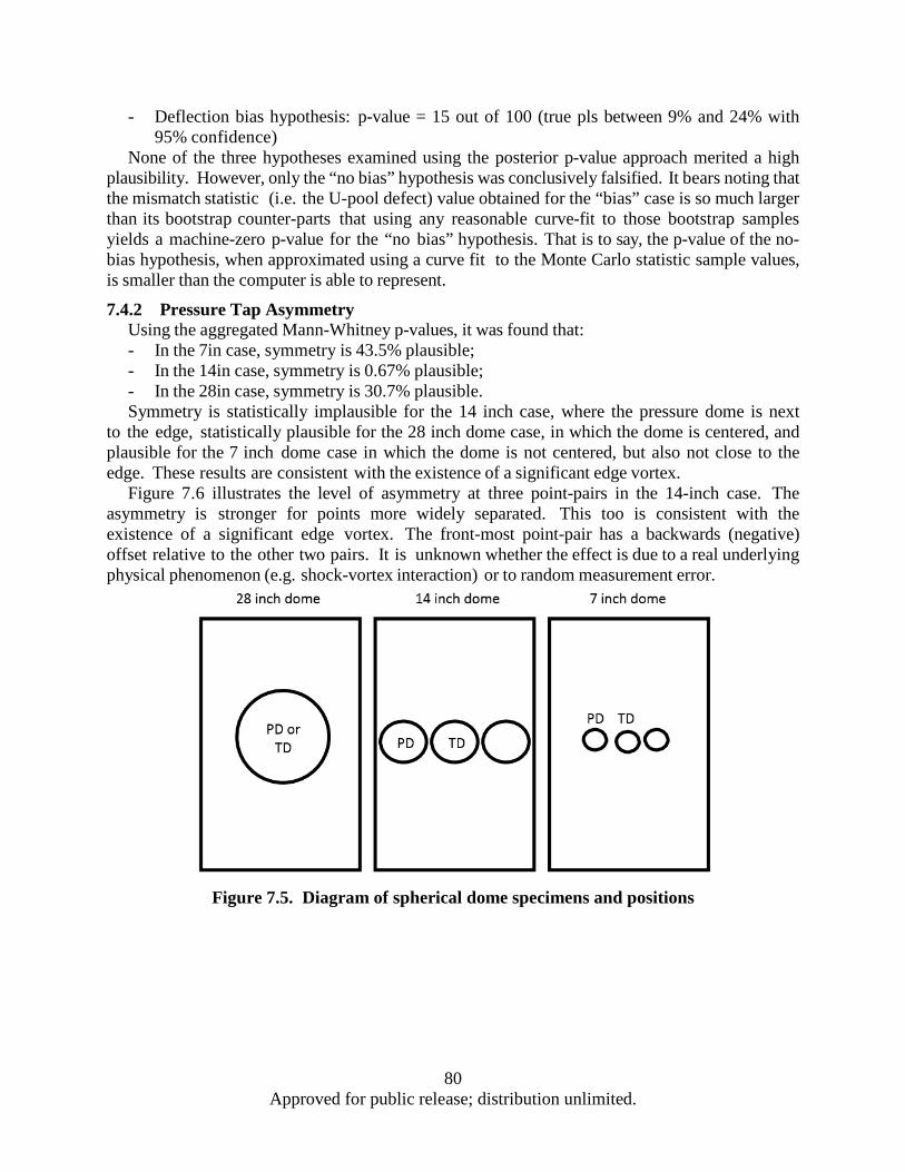
- Deflection bias hypothesis: p-value = 15 out of 100 (true pls between 9% and 24% with 95% confidence)
None of the three hypotheses examined using the posterior p-value approach merited a high plausibility. However, only the “no bias” hypothesis was conclusively falsified. It bears noting that the mismatch statistic (i.e. the U-pool defect) value obtained for the “bias” case is so much larger than its bootstrap counter-parts that using any reasonable curve-fit to those bootstrap samples yields a machine-zero p-value for the “no bias” hypothesis. That is to say, the p-value of the no-bias hypothesis, when approximated using a curve fit to the Monte Carlo statistic sample values, is smaller than the computer is able to represent.
7.4.2 Pressure Tap Asymmetry Using the aggregated Mann-Whitney p-values, it was found that: - In the 7in case, symmetry is 43.5% plausible; - In the 14in case, symmetry is 0.67% plausible; - In the 28in case, symmetry is 30.7% plausible. Symmetry is statistically implausible for the 14 inch case, where the pressure dome is next
to the edge, statistically plausible for the 28 inch dome case, in which the dome is centered, and plausible for the 7 inch dome case in which the dome is not centered, but also not close to the edge. These results are consistent with the existence of a significant edge vortex.
Figure 7.6 illustrates the level of asymmetry at three point-pairs in the 14-inch case. The asymmetry is stronger for points more widely separated. This too is consistent with the existence of a significant edge vortex. The front-most point-pair has a backwards (negative) offset relative to the other two pairs. It is unknown whether the effect is due to a real underlying physical phenomenon (e.g. shock-vortex interaction) or to random measurement error.
Figure 7.5. Diagram of spherical dome specimens and positions
80 Approved for public release; distribution unlimited.
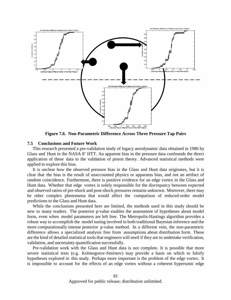
Figure 7.6. Non-Parametric Difference Across Three Pressure Tap Pairs
7.5 Conclusions and Future Work This research presented a pre-validation study of legacy aerodynamic data obtained in 1986 by
Glass and Hunt in the NASA 8’ HTT. An apparent bias in the pressure data confounds the direct application of these data to the validation of piston theory. Advanced statistical methods were applied to explore this bias.
It is unclear how the observed pressure bias in the Glass and Hunt data originates, but it is clear that the bias is the result of unaccounted physics or apparatus bias, and not an artifact of random coincidence. Furthermore, there is positive evidence for an edge vortex in the Glass and Hunt data. Whether that edge vortex is solely responsible for the discrepancy between expected and observed ratios of pre-shock and post-shock pressures remains unknown. Moreover, there may be other complex phenomena that would affect the comparison of reduced-order model predictions to the Glass and Hunt data.
While the conclusions presented here are limited, the methods used in this study should be new to many readers. The posterior p-value enables the assessment of hypotheses about model form, even when model parameters are left free. The Metropolis-Hastings algorithm provides a robust way to accomplish the model tuning involved in both traditional Bayesian inference and the more computationally intense posterior p-value method. In a different vein, the non-parametric difference allows a specialized analysis free from assumptions about distribution form. These are the kind of detailed statistical tools that engineers will need if they are to undertake verification, validation, and uncertainty quantification successfully.
Pre-validation work with the Glass and Hunt data is not complete. It is possible that more severe statistical tests (e.g. Kolmogorov-Smirnov) may provide a basis on which to falsify hypotheses explored in this study. Perhaps more important is the problem of the edge vortex. It is impossible to account for the effects of an edge vortex without a coherent hypersonic edge
81 Approved for public release; distribution unlimited.

vortex model. To the authors’ knowledge, this remains one of the outstanding problems in aerodynamics.
While there will certainly be some point at which the analyst must say “enough is enough,” right now, the unexplained discrepancies in the Glass and Hunt data are too large to ignore. Moreover, it is anticipated that legacy hypersonic wind tunnel data are replete with such discrepancies. The wind tunnel engineers of previous decades simply did not design their experiments with quantitative model validation in mind. However, judicious pre-validation studies, like the one commenced here, may ultimately provide a framework for using those legacy data in today’s validation efforts.
82 Approved for public release; distribution unlimited.

8 UNCERTAINTY QUANTIFICATION OF STATE BOUNDARIES IN THIN BEAM BUCKLING EXPERIMENTS
State selection – or model selection – has garnered interest in many fields including phylogenetics [73], social research [74], ecology and evolution [75], protein evolution [76], and data mining [77]. Selection of the best model is based either on classical hypothesis testing, information theoretic measures, or Bayesian hypothesis testing. Classical approaches test likelihood ratio statistics to find the best model [78]. Information theoretic measures are the Akaike information criterion (AIC) [79] and its generalization Network information criterion (NIC) [80], corrected Akaike information criterion (AICC) [81], the focused information criterion (FIC) [82], the Kullback-Leibler information criterion (KLIC) [83], Takeuchi information criterion (TIC) [84], minimum description length (MDL) [85], and deviance information criterion (DIC) [86]. The popular Schwarz Bayesian information criterion (BIC) [87] is not an information theoretic measure and was originally derived to select the posterior most probable model. BIC is often taken as an approximation to Bayes factors [88], which are an element of the Bayesian posterior odds ratio. Bayes factors, and by extension, posterior odds, are a natural implementation of Occam’s razor [89], and require no modifications for model complexity. No assumptions about nested models or estimates of model complexity are required, as with many non-Bayesian methods. Further, they are suitable for comparing multiple hypotheses (i.e. models), where most classical statistical methodologies only compare two hypotheses. Computation of a Bayesian posterior odds [90] does require prior distributions for parameters (or prior probabilities for models) to be assumed, which can be a difficult task. Quantifying model selection uncertainty is straightforward from the Bayesian posterior odds ratio, which yields posterior probabilities for each model which can then be used to rank the models[88,91]. Bayesian model averaging [92], which mitigates overconfidence in the model, follows naturally. Note that estimation of model selection uncertainty, however, is also possible using model selection criterion such as AIC or BIC. These criteria compute model weights that can be interpreted as probabilities.
State boundary uncertainty quantification (SBUQ) quantifies the uncertainty in a boundary between two states, as opposed to the uncertainty in model selection. SBUQ, of course, requires knowledge of the model selection uncertainty. Previous work on this problem includes that of Hombal and Mahadevan [98], who developed a probabilistic treatment of model selection using error surrogates that considers uncertainty in the classification boundary. Alternative formulations of the SBUQ problem may be possible, each with their own pros and cons. Stochastic optimization can provide a distribution of the critical boundary value while being a simpler overall methodology, but do not provide a direct means for belief updating in the presence of new information. Discriminative classification techniques (e.g., logistic regression [99], neural networks [100], support vector machines [101], relevance vector machines [102]) may provide a means of obtaining an estimate of the discrete state with an associated confidence by regressing on discrete and continuous system inputs. Generative classification techniques (e.g., Gaussian discriminative analysis [103]) compare likelihoods between competing models to estimate the discrete state. However, individually, either style of classification may not account for enough information to confidently determine the state. Discriminative methods may assume an incorrect causal interpretation of the system (i.e., responses do not cause the discrete state) and pose difficulties when the regressor variables are not independent. Generative methods require stronger assumptions about the underlying distribution of the data than discriminative
83 Approved for public release; distribution unlimited.
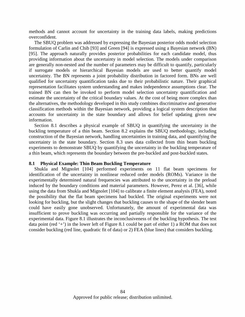
methods and cannot account for uncertainty in the training data labels, making predictions overconfident.
The SBUQ problem was addressed by expressing the Bayesian posterior odds model selection formulation of Carlin and Chib [93] and Green [94] is expressed using a Bayesian network (BN) [95]. The approach naturally provides posterior probabilities for each candidate model, thus providing information about the uncertainty in model selection. The models under comparison are generally non-nested and the number of parameters may be difficult to quantify, particularly if surrogate models or hierarchical Bayesian models are used to better quantify model uncertainty. The BN represents a joint probability distribution in factored form. BNs are well qualified for uncertainty quantification tasks due to their probabilistic nature. Their graphical representation facilitates system understanding and makes independence assumptions clear. The trained BN can then be invoked to perform model selection uncertainty quantification and estimate the uncertainty of the critical boundary values. At the cost of being more complex than the alternatives, the methodology developed in this study combines discriminative and generative classification methods within the Bayesian network, providing a logical system description that accounts for uncertainty in the state boundary and allows for belief updating given new information.
Section 8.1 describes a physical example of SBUQ in quantifying the uncertainty in the buckling temperature of a thin beam. Section 8.2 explains the SBUQ methodology, including construction of the Bayesian network, handling uncertainties in training data, and quantifying the uncertainty in the state boundary. Section 8.3 uses data collected from thin beam buckling experiments to demonstrate SBUQ by quantifying the uncertainty in the buckling temperature of a thin beam, which represents the boundary between the pre-buckled and post-buckled states.
8.1 Physical Example: Thin Beam Buckling Temperature Shukla and Mignolet [104] performed experiments on 11 flat beam specimens for
identification of the uncertainty in nonlinear reduced order models (ROMs). Variance in the experimentally determined natural frequencies was attributed to the uncertainty in the preload induced by the boundary conditions and material parameters. However, Perez et al. [36], while using the data from Shukla and Mignolet [104] to calibrate a finite element analysis (FEA), noted the possibility that the flat beam specimens had buckled. The original experiments were not looking for buckling, but the slight changes that buckling causes to the shape of the slender beam could have easily gone unobserved. Unfortunately, the amount of experimental data was insufficient to prove buckling was occurring and partially responsible for the variance of the experimental data. Figure 8.1 illustrates the inconclusiveness of the buckling hypothesis. The test data point (red ‘+’) in the lower left of Figure 8.1 could be part of either 1) a ROM that does not consider buckling (red line, quadratic fit of data) or 2) FEA (blue lines) that considers buckling.
84 Approved for public release; distribution unlimited.

Figure 8.1. Shukla and Mignolet [104] experimental results compared to finite element
analysis for pre- and post-buckled operating states.
In an attempt to determine which explanation was best and create a better model, a new experiment for the flat beam was designed. The focus of these tests was to reduce uncertainty induced by the boundary conditions and provide sufficient data for calibrating the FEA and determining the presence of buckling. This was achieved by using a single beam specimen that remained clamped in place throughout the experiment. The beam was repeatedly heated until a steady state temperature was reached, then it was allowed to cool. Measurements were obtained as the beam cooled. While distinct pre- and post-buckled behavior was not the focus of the Shukla and Mignolet [104] experiments, Perez et al. [36] investigated and confirmed this phenomenon. The case study presented in Section 8.3 uses this data to quantify the uncertainty in the buckling temperature using the state boundary uncertainty quantification methodology.
The theoretical Euler buckling load of a column, 𝐹𝐹𝑐𝑐𝑐𝑐, may be calculated using classical mechanics by
𝐹𝐹𝑐𝑐𝑐𝑐 =𝜋𝜋2𝐸𝐸𝐸𝐸𝐿𝐿𝑒𝑒2
(8.1)
where E is the modulus of elasticity, I is the minimum moment of inertia of the cross sectional area, and 𝐿𝐿𝑒𝑒 is the effective length of the column considering the boundary conditions. For a column with both ends fixed, the effective length is 𝐿𝐿𝑒𝑒 = 0.5𝐿𝐿, where L is the actual column length. For this research, critical buckling temperature is of interest. The force induced by a temperature load on a beam fixed at both ends is 𝐹𝐹𝑇𝑇 = −𝐸𝐸𝐸𝐸𝐸𝐸(𝑇𝑇0 − 𝑇𝑇) (8.2)
85
Approved for public release; distribution unlimited.
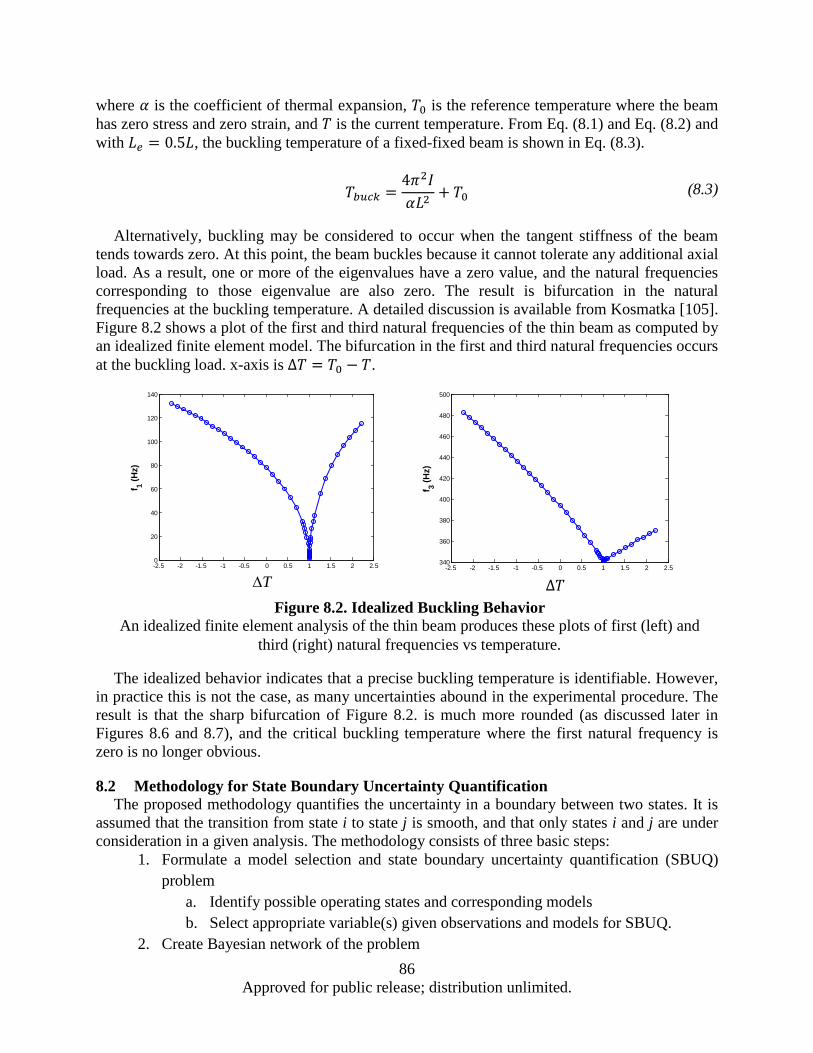
where 𝐸𝐸 is the coefficient of thermal expansion, 𝑇𝑇0 is the reference temperature where the beam has zero stress and zero strain, and 𝑇𝑇 is the current temperature. From Eq. (8.1) and Eq. (8.2) and with 𝐿𝐿𝑒𝑒 = 0.5𝐿𝐿, the buckling temperature of a fixed-fixed beam is shown in Eq. (8.3).
𝑇𝑇𝑏𝑏𝑏𝑏𝑐𝑐𝑏𝑏 =4𝜋𝜋2𝐸𝐸𝐸𝐸𝐿𝐿2
+ 𝑇𝑇0 (8.3)
Alternatively, buckling may be considered to occur when the tangent stiffness of the beam
tends towards zero. At this point, the beam buckles because it cannot tolerate any additional axial load. As a result, one or more of the eigenvalues have a zero value, and the natural frequencies corresponding to those eigenvalue are also zero. The result is bifurcation in the natural frequencies at the buckling temperature. A detailed discussion is available from Kosmatka [105]. Figure 8.2 shows a plot of the first and third natural frequencies of the thin beam as computed by an idealized finite element model. The bifurcation in the first and third natural frequencies occurs at the buckling load. x-axis is ∆𝑇𝑇 = 𝑇𝑇0 − 𝑇𝑇.
The idealized behavior indicates that a precise buckling temperature is identifiable. However,
in practice this is not the case, as many uncertainties abound in the experimental procedure. The result is that the sharp bifurcation of Figure 8.2. is much more rounded (as discussed later in Figures 8.6 and 8.7), and the critical buckling temperature where the first natural frequency is zero is no longer obvious.
8.2 Methodology for State Boundary Uncertainty Quantification The proposed methodology quantifies the uncertainty in a boundary between two states. It is
assumed that the transition from state i to state j is smooth, and that only states i and j are under consideration in a given analysis. The methodology consists of three basic steps:
1. Formulate a model selection and state boundary uncertainty quantification (SBUQ) problem
a. Identify possible operating states and corresponding models b. Select appropriate variable(s) given observations and models for SBUQ.
2. Create Bayesian network of the problem
∆T ∆𝑇𝑇
Figure 8.2. Idealized Buckling Behavior An idealized finite element analysis of the thin beam produces these plots of first (left) and
third (right) natural frequencies vs temperature.
-2.5 -2 -1.5 -1 -0.5 0 0.5 1 1.5 2 2.50
20
40
60
80
100
120
140
f 1 (Hz)
-2.5 -2 -1.5 -1 -0.5 0 0.5 1 1.5 2 2.5340
360
380
400
420
440
460
480
500
( )
f 3 (Hz)
86 Approved for public release; distribution unlimited.

a. Define graphical structure corresponding to model selection problem b. Prepare training data for BN c. Estimate BN distribution parameters
3. Quantify state boundary uncertainty a. Estimate probability of system being in each operating state with respect to a
particular measurement via inference Features of the methodology are illustrated throughout this section using the thin beam
problem. In this problem, a thin beam subjected to temperature load may be in either a pre-buckled or post-buckled configuration. Due to many sources of uncertainty, discussed in Section 8.3, it is difficult to determine the exact buckling temperature of the beam, so the distribution of the buckling temperature is sought.
8.2.1 Probabilistic Model Selection Consider a problem domain over the variables 𝐱𝐱 ∈ x1, … , 𝑑𝑑𝑛𝑛. x consists of two subsets, the
set of r observable variables 𝐱𝐱 ∈ z1, … , z𝑐𝑐 and the set of of p unobservable (hidden) variables 𝐡𝐡 ∈ ℎ1, … ,ℎ𝑝𝑝 such that 𝑛𝑛 = 𝑃𝑃 + 𝑝𝑝. For example, z1 could represent a measurable quantity such as velocity or natural frequency while x1 could represent an unobservable system variable such as an operating mode, health state, or even measurable quantities for which no measurements are available. A single realization of zi is denoted by Zi ∋ 𝒁𝒁and a single realization of xi by Xi. ∋ 𝑿𝑿 For the model selection formulation, a variable 𝑀𝑀 ∋ 𝐡𝐡, represents a choice of system model (operating mode) that cannot be directly measured or observed. As such, the value of M, i.e., M = m1 and M = m2, must be inferred by considering the measured variables z.
The critical value of measurement variable 𝑧𝑧𝑖𝑖, denoted 𝑧𝑧𝑖𝑖𝑐𝑐, is the boundary between two states (models) M = m1 and M = m2 along dimension 𝑧𝑧𝑖𝑖. For example, 𝑧𝑧𝑖𝑖𝑐𝑐 could, refer to the stress at which a material switches from elastic to plastic behavior. Estimating 𝑃𝑃𝑃𝑃𝑀𝑀 = 𝑚𝑚𝑗𝑗𝐙𝐙 over a range of 𝑧𝑧𝑖𝑖 presumed to contain 𝑧𝑧𝑖𝑖𝑐𝑐 provides the information to estimate the distribution of 𝑧𝑧𝑖𝑖𝑐𝑐, 𝑝(𝑧𝑧𝑖𝑖𝑐𝑐). The estimation of 𝑃𝑃𝑃𝑃𝑀𝑀 = 𝑚𝑚𝑗𝑗𝐙𝐙 may be viewed through the Bayes factor and probabilistic model selection.
Given observations Z and model choices M = m1 and M = m2, the ratio of posterior odds for competing models is
𝑃𝑃𝑃𝑃(𝑀𝑀 = 𝑚𝑚1|𝒁𝒁)𝑃𝑃𝑃𝑃(𝑀𝑀 = 𝑚𝑚2|𝒁𝒁) =
𝑃𝑃𝑃𝑃(𝒁𝒁|𝑀𝑀 = 𝑚𝑚1)𝑃𝑃𝑃𝑃(𝒁𝒁|𝑀𝑀 = 𝑚𝑚2) ×
𝑃𝑃𝑃𝑃(𝑀𝑀 = 𝑚𝑚1)𝑃𝑃𝑃𝑃(𝑀𝑀 = 𝑚𝑚2) (8.4)
The first term on the right hand side is the Bayes factor, 𝐵𝐵𝑖𝑖𝑗𝑗, and the second term is the ratio of prior odds. Thus, the Bayes factor is the ratio of prior to posterior odds. When 𝑃𝑃𝑃𝑃(𝑀𝑀 = 𝑚𝑚1) =𝑃𝑃𝑃𝑃(𝑀𝑀 = 𝑚𝑚2), the Bayes factor is the posterior odds ratio. When the posterior odds ratio is equal to 1, both models are equally likely. As 𝐵𝐵12 increases, the evidence against M = m2 increases, providing a basis for model selection.
A probabilistic model selection problem can be formulated where the model choice is included as a discrete random variable [93,94]. Suppose the problem is to select from amongst K possible model choices, each with parameter vector 𝜽𝜽𝑗𝑗 , 𝑗𝑗 = 1, … ,𝐾𝐾. Let y be a vector of observable system responses. Using a Bayesian model specification, the prior probability of the models is 𝜋𝜋𝑗𝑗 = 𝑃𝑃𝑃𝑃 (𝑀𝑀 = 𝑚𝑚𝑗𝑗), with ∑ 𝜋𝜋𝑗𝑗𝐾𝐾
𝑗𝑗=1 = 1. The model parameters 𝜽𝜽𝑗𝑗 are conditioned on M
87 Approved for public release; distribution unlimited.
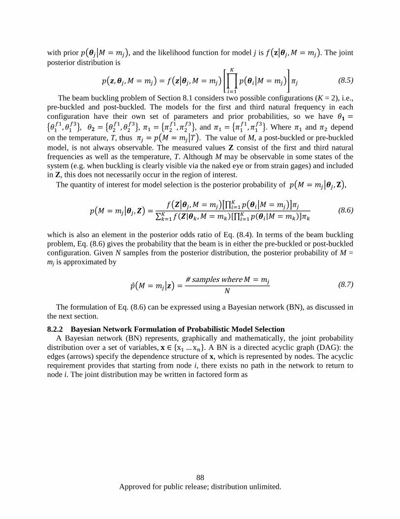
with prior 𝑝𝑝𝜽𝜽𝑗𝑗𝑀𝑀 = 𝑚𝑚𝑗𝑗, and the likelihood function for model j is 𝑓𝑓𝐳𝐳𝜽𝜽𝑗𝑗 ,𝑀𝑀 = 𝑚𝑚𝑗𝑗. The joint posterior distribution is
𝑝𝑝𝒛𝒛,𝜽𝜽𝑗𝑗 ,𝑀𝑀 = 𝑚𝑚𝑗𝑗 = 𝑓𝑓𝒛𝒛𝜽𝜽𝑗𝑗 ,𝑀𝑀 = 𝑚𝑚𝑗𝑗 𝑝𝑝𝜽𝜽𝑖𝑖𝑀𝑀 = 𝑚𝑚𝑗𝑗𝐾𝐾
𝑖𝑖=1
𝜋𝜋𝑗𝑗 (8.5)
The beam buckling problem of Section 8.1 considers two possible configurations (K = 2), i.e., pre-buckled and post-buckled. The models for the first and third natural frequency in each configuration have their own set of parameters and prior probabilities, so we have 𝜃𝜃𝟏𝟏 =𝜃𝜃1
𝑓𝑓1,𝜃𝜃1𝑓𝑓3, 𝜃𝜃𝟐𝟐 = 𝜃𝜃2
𝑓𝑓1,𝜃𝜃2𝑓𝑓3, 𝜋𝜋1 = 𝜋𝜋2
𝑓𝑓1,𝜋𝜋2𝑓𝑓3, and 𝜋𝜋1 = 𝜋𝜋1
𝑓𝑓1,𝜋𝜋1𝑓𝑓3. Where 𝜋𝜋1 and 𝜋𝜋2 depend
on the temperature, T, thus 𝜋𝜋𝑗𝑗 = 𝑝𝑝𝑀𝑀 = 𝑚𝑚𝑗𝑗𝑇𝑇. The value of M, a post-buckled or pre-buckled model, is not always observable. The measured values Z consist of the first and third natural frequencies as well as the temperature, T. Although M may be observable in some states of the system (e.g. when buckling is clearly visible via the naked eye or from strain gages) and included in Z, this does not necessarily occur in the region of interest.
The quantity of interest for model selection is the posterior probability of 𝑝𝑝𝑀𝑀 = 𝑚𝑚𝑗𝑗𝜽𝜽𝑗𝑗 ,𝐙𝐙,
𝑝𝑝𝑀𝑀 = 𝑚𝑚𝑗𝑗𝜽𝜽𝑗𝑗 ,𝒁𝒁 =𝑓𝑓𝒁𝒁𝜽𝜽𝑗𝑗 ,𝑀𝑀 = 𝑚𝑚𝑗𝑗∏ 𝑝𝑝𝜽𝜽𝑖𝑖𝑀𝑀 = 𝑚𝑚𝑗𝑗𝐾𝐾
𝑖𝑖=1 𝜋𝜋𝑗𝑗∑ 𝑓𝑓(𝒁𝒁|𝜽𝜽𝑏𝑏 ,𝑀𝑀 = 𝑚𝑚𝑏𝑏)[∏ 𝑝𝑝(𝜽𝜽𝑖𝑖|𝑀𝑀 = 𝑚𝑚𝑏𝑏)𝐾𝐾
𝑖𝑖=1 ]𝜋𝜋𝑏𝑏𝐾𝐾𝑏𝑏=1
(8.6)
which is also an element in the posterior odds ratio of Eq. (8.4). In terms of the beam buckling problem, Eq. (8.6) gives the probability that the beam is in either the pre-buckled or post-buckled configuration. Given N samples from the posterior distribution, the posterior probability of M = mj is approximated by
𝑝𝑀𝑀 = 𝑚𝑚𝑗𝑗𝒛𝒛 =# samples where 𝑀𝑀 = 𝑚𝑚𝑗𝑗
𝑁𝑁 (8.7)
The formulation of Eq. (8.6) can be expressed using a Bayesian network (BN), as discussed in
the next section.
8.2.2 Bayesian Network Formulation of Probabilistic Model Selection A Bayesian network (BN) represents, graphically and mathematically, the joint probability
distribution over a set of variables, 𝐱𝐱 ∈ x1 … x𝑛𝑛. A BN is a directed acyclic graph (DAG): the edges (arrows) specify the dependence structure of x, which is represented by nodes. The acyclic requirement provides that starting from node i, there exists no path in the network to return to node i. The joint distribution may be written in factored form as
88 Approved for public release; distribution unlimited.
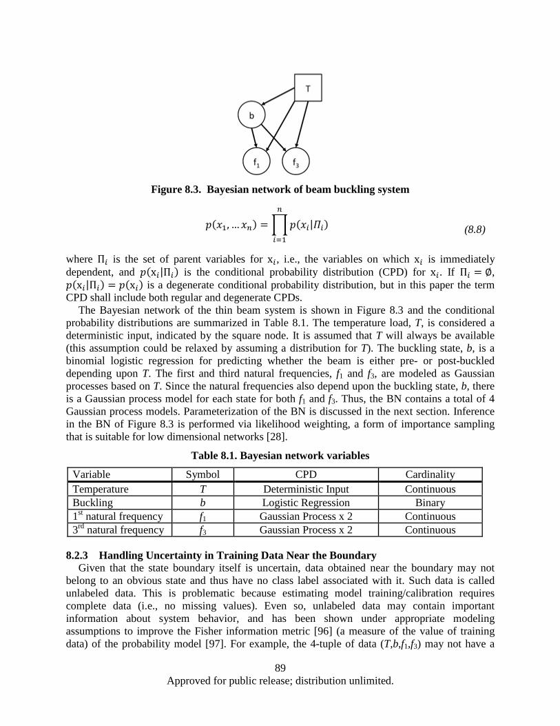
Figure 8.3. Bayesian network of beam buckling system
𝑝𝑝(𝑑𝑑1, … 𝑑𝑑𝑛𝑛) = 𝑝𝑝(𝑑𝑑𝑖𝑖|𝛱𝛱𝑖𝑖)
𝑛𝑛
𝑖𝑖=1
(8.8)
where Π𝑖𝑖 is the set of parent variables for x𝑖𝑖, i.e., the variables on which x𝑖𝑖 is immediately dependent, and 𝑝𝑝(x𝑖𝑖|Π𝑖𝑖) is the conditional probability distribution (CPD) for x𝑖𝑖. If Π𝑖𝑖 = ∅, 𝑝𝑝(x𝑖𝑖|Π𝑖𝑖) = 𝑝𝑝(x𝑖𝑖) is a degenerate conditional probability distribution, but in this paper the term CPD shall include both regular and degenerate CPDs.
The Bayesian network of the thin beam system is shown in Figure 8.3 and the conditional probability distributions are summarized in Table 8.1. The temperature load, T, is considered a deterministic input, indicated by the square node. It is assumed that T will always be available (this assumption could be relaxed by assuming a distribution for T). The buckling state, b, is a binomial logistic regression for predicting whether the beam is either pre- or post-buckled depending upon T. The first and third natural frequencies, f1 and f3, are modeled as Gaussian processes based on T. Since the natural frequencies also depend upon the buckling state, b, there is a Gaussian process model for each state for both f1 and f3. Thus, the BN contains a total of 4 Gaussian process models. Parameterization of the BN is discussed in the next section. Inference in the BN of Figure 8.3 is performed via likelihood weighting, a form of importance sampling that is suitable for low dimensional networks [28].
8.2.3 Handling Uncertainty in Training Data Near the Boundary
Given that the state boundary itself is uncertain, data obtained near the boundary may not belong to an obvious state and thus have no class label associated with it. Such data is called unlabeled data. This is problematic because estimating model training/calibration requires complete data (i.e., no missing values). Even so, unlabeled data may contain important information about system behavior, and has been shown under appropriate modeling assumptions to improve the Fisher information metric [96] (a measure of the value of training data) of the probability model [97]. For example, the 4-tuple of data (T,b,f1,f3) may not have a
Table 8.1. Bayesian network variables
Variable Symbol CPD Cardinality Temperature T Deterministic Input Continuous Buckling b Logistic Regression Binary 1st natural frequency f1 Gaussian Process x 2 Continuous 3rd natural frequency f3 Gaussian Process x 2 Continuous
89 Approved for public release; distribution unlimited.
value of b, but still have values for f1 and f3 that can be used for analysis. This situation occurs near the state transition boundary because it is difficult to pinpoint the exact moment when buckling occurs on a vibrating beam specimen.
Figure 8.4. The labeling boundary is a weighted average of the temperatures at which the f1
and f3 mean functions are at their respective minimums
In the thin beam problem, the state transition boundary corresponds to the temperature at which the natural frequencies are at their minimum. Figure 8.4 shows the mean Gaussian Process (GP) model responses (with ΔT as the independent variable) constructed from the training data for f1 and f3. No labels for pre- or post-buckling are required to fit these GP models. The threshold ΔT value for classification is unclear because, as seen in Figure 8.4, the mean curves for f1 and f3 have minimum values at different temperatures, (∆𝑇𝑇1′ and ∆𝑇𝑇3′). This is an indicator of the uncertainty in the buckling temperature and the reason for being unable to confidently label the data in the first place. To account for the uncertainty in the training data, a variance weighted labeling threshold ∆𝑇𝑇𝑡𝑡ℎ𝑐𝑐𝑒𝑒𝑟𝑟ℎ = 𝑑𝑑1∆𝑇𝑇1′ + 𝑑𝑑3∆𝑇𝑇3′ is estimated, where 𝑑𝑑1 = 1 −𝜎𝜎12′ (𝜎𝜎12′ + 𝜎𝜎32′)⁄ and 𝑑𝑑3 = 1 − 𝜎𝜎32′ (𝜎𝜎12′ + 𝜎𝜎32′)⁄ . the variances at both minimums (𝜎𝜎12′ and 𝜎𝜎32′) are calculated from the GP models. The training data can now be labeled as either pre- or post-buckled using the class boundary, and the 4 GP models describing f1 and f3 in the pre- and post-buckled states can now be trained. These GP models may be built with standard covariance functions, such as the Matern class and trained using maximum likelihood estimation or Bayesian methods.
Even with an estimate of the labeling threshold, these GP models include little information about the confidence in the labels assigned to the training data. This labeling uncertainty is accounted for in the BN by the logistic regression: the likelihoods of the f1 and f3 predictions will be combined with the probability of being pre- or post-buckled during Bayesian updating in the BN, as determined by a logistic regression, represented by b in the Bayesian network of Figure 8.3. The logistic regression computes the probability of being either pre- or post-buckled as a function of temperature. The probability effectively weights the confidence in the responses from the GP model at a given temperature.
90 Approved for public release; distribution unlimited.
The regression of a training set of m labeled examples 𝑑𝑑(1),𝑦𝑦(1), … , 𝑑𝑑(𝑚𝑚),𝑦𝑦(𝑚𝑚), where the discrete variable 𝑦𝑦(𝑖𝑖) has k possible outcomes and 𝑑𝑑(𝑖𝑖) ∈ ℝ𝑛𝑛+1 with x0 = 1 as the intercept may be described by
ℎ𝜃𝜃𝑑𝑑(𝑖𝑖) =
⎣⎢⎢⎢⎡𝑝𝑝𝑦𝑦
(𝑖𝑖) = 1𝑑𝑑(𝑖𝑖),𝜃𝜃𝑝𝑝𝑦𝑦(𝑖𝑖) = 2𝑑𝑑(𝑖𝑖),𝜃𝜃
⋮𝑝𝑝𝑦𝑦(𝑖𝑖) = 𝑘𝑘𝑑𝑑(𝑖𝑖),𝜃𝜃⎦
⎥⎥⎥⎤
=1
∑ 𝑒𝑒𝜃𝜃𝑗𝑗𝑇𝑇𝑥𝑥(𝑖𝑖)𝑏𝑏
𝑗𝑗=1 ⎣⎢⎢⎡𝑒𝑒
𝜃𝜃1𝑇𝑇𝑥𝑥(𝑖𝑖)
𝑒𝑒𝜃𝜃2𝑇𝑇𝑥𝑥(𝑖𝑖)
⋮𝑒𝑒𝜃𝜃𝑘𝑘
𝑇𝑇𝑥𝑥(𝑖𝑖)⎦⎥⎥⎤ (8.9)
with parameters Θ = 𝜃𝜃1,𝜃𝜃2, … ,𝜃𝜃𝑏𝑏and normalizing term 1 ∑ 𝑒𝑒𝜃𝜃𝑗𝑗
𝑇𝑇𝑥𝑥(𝑖𝑖)𝑏𝑏𝑗𝑗=1⁄ . If k = 2, this is a logistic
regression, and if k > 2, the regression is termed a multinomial logistic regression or softmax regression [99].
Typically, the data for training the logistic regression would consist of labeled data where the gradual change in probability of observing the different classes is reflected in the training data. However, since the training data was labeled using an abrupt boundary, a logistic regression fitted to the training data will reflect this by having a sharp boundary between classes. The gradual transition between classes expected to arise due to experimental uncertainties will not be present. However, a process called L2 regularization (or variously Tikhonov [106] regularization or ridge regression [107]) provides a means of controlling the sharpness of the class boundary. L2 regularization is often used to limit model complexity by adding a weight decay term to the cost function being minimized during regression. Increasing the size of the penalty has the effect of smoothing the model. The weight decay term is often found via cross-validation to find the model that achieves the best predictive performance. Equation (8.10) shows the cost function for logistic regression with a weight decay term with parameter λ added on the right hand side. Equation (8.10) is minimized for a given λ to find the optimal parameters Θ.
𝐽𝐽(𝜃𝜃) = −1𝑚𝑚𝐸𝐸𝑦𝑦(𝑖𝑖) = 𝑗𝑗𝑙𝑙𝑙𝑙𝑙𝑙
𝑒𝑒𝜃𝜃𝑗𝑗𝑇𝑇𝑥𝑥(𝑖𝑖)
∑ 𝑒𝑒𝜃𝜃𝑙𝑙𝑇𝑇𝑥𝑥(𝑖𝑖)𝑏𝑏𝑙𝑙=1
𝑏𝑏
𝑗𝑗=1
𝑚𝑚
𝑖𝑖=1
+𝜆𝜆2𝜃𝜃𝑖𝑖𝑗𝑗2
𝑛𝑛
𝑗𝑗=0
𝑏𝑏
𝑖𝑖=1
(8.10)
In this study, the weight decay term is varied until the resulting logistic regression fits the
expert’s beliefs about the probability of being in the post-buckling condition at a particular temperature (e.g., 1% probability at ΔT = 7° C). The expert would make this judgment qualitatively or by employing heuristics, the goal being to capture the region of classification uncertainty. Then, by finding the temperature corresponding to 50% probability, symmetry can be used to find the boundary on the other side, as the logistic regression assumes the log odds of the probability varies linearly. This procedure provides a means to fuse expert opinion into the methodology.
91 Approved for public release; distribution unlimited.

8.2.4 Quantification of State Boundary Uncertainty With a trained BN available, the model variable, M, can be inferred. Given some set of
measurements, Z, that does not include the model variable M, the inference algorithm is run with N samples to estimate 𝑝𝑀𝑀 = 𝑚𝑚𝑗𝑗𝐙𝐙 for all j. Of course, Z represents only one instantiation of the measured variables. Thus, 𝑝𝑀𝑀 = 𝑚𝑚𝑗𝑗𝐙𝐙 is only a point estimate of probabilities of 𝑀𝑀 = 𝑚𝑚𝑗𝑗. To determine the distribution of the boundary, 𝑝(𝑧𝑧𝑖𝑖𝑐𝑐), the value of 𝑝𝑀𝑀 = 𝑚𝑚𝑗𝑗𝐙𝐙 must be computed via inference over a range of values for 𝑧𝑧𝑖𝑖. While 𝑧𝑧𝑖𝑖 values are selected to represent a range of 𝑧𝑧𝑖𝑖, no selection criteria is extended to 𝑧𝑧¬𝑖𝑖 (¬𝑖𝑖 refers to all indices except i). Figure 8.5 illustrates how the probability of M being in one of two states changes with a variable 𝑧𝑧𝑖𝑖 and the resulting distribution of 𝑧𝑧𝑖𝑖𝑐𝑐.
In the beam buckling problem, 𝑝(𝑧𝑧𝑖𝑖𝑐𝑐) is the distribution of the buckling temperature, which is
estimated by evaluating the probability of the model being in the pre-buckled or post-buckled state at predetermined temperature values. Temperature is the 𝑧𝑧𝑖𝑖 variable and the first and third natural frequencies, f1 and f3, are the 𝑧𝑧¬𝑖𝑖 variables, which are allowed to vary.
8.2.5 Methodology Summary A methodology was developed for the quantification of state boundary uncertainty. First, a
model selection problem is developed. The model selection problem is then formulated as a BN. Data near the boundary is classified using an optimization algorithm. The BN may then be trained. Finally, inference is performed in the BN for a range of values of the variable of interest. A probability distribution of the state boundary is then constructed. Next, a case study is used to demonstrate the methodology.
8.3 Case Study: Thin Beam Buckling Section 8.2 outlined a methodology for quantifying the uncertainty in the state boundary,
which is applied in this section for the pre- and post-buckled states of a thin beam subjected to a thermal load.
8.3.1 Experimental Procedure Due to the difficulty of observing buckling temperature directly with any reasonable
confidence (particularly in the region of interest), Perez et al.38 developed an experiment to measure the natural frequencies of a thin steel beam.
Figure 8.5. State boundary uncertainty
Left: Pr(M = m1) and Pr(M = m2) vary as the boundary x = 0 is approached. Right: The distribution of the critical z value that marks the boundary between M = m1 and M = m2.
92 Approved for public release; distribution unlimited.
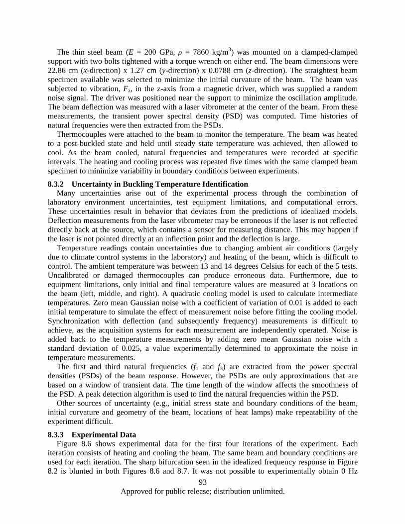
The thin steel beam (E = 200 GPa, ρ = 7860 kg/m3) was mounted on a clamped-clamped support with two bolts tightened with a torque wrench on either end. The beam dimensions were 22.86 cm (x-direction) x 1.27 cm (y-direction) x 0.0788 cm (z-direction). The straightest beam specimen available was selected to minimize the initial curvature of the beam. The beam was subjected to vibration, Fz, in the z-axis from a magnetic driver, which was supplied a random noise signal. The driver was positioned near the support to minimize the oscillation amplitude. The beam deflection was measured with a laser vibrometer at the center of the beam. From these measurements, the transient power spectral density (PSD) was computed. Time histories of natural frequencies were then extracted from the PSDs.
Thermocouples were attached to the beam to monitor the temperature. The beam was heated to a post-buckled state and held until steady state temperature was achieved, then allowed to cool. As the beam cooled, natural frequencies and temperatures were recorded at specific intervals. The heating and cooling process was repeated five times with the same clamped beam specimen to minimize variability in boundary conditions between experiments.
8.3.2 Uncertainty in Buckling Temperature Identification Many uncertainties arise out of the experimental process through the combination of
laboratory environment uncertainties, test equipment limitations, and computational errors. These uncertainties result in behavior that deviates from the predictions of idealized models. Deflection measurements from the laser vibrometer may be erroneous if the laser is not reflected directly back at the source, which contains a sensor for measuring distance. This may happen if the laser is not pointed directly at an inflection point and the deflection is large.
Temperature readings contain uncertainties due to changing ambient air conditions (largely due to climate control systems in the laboratory) and heating of the beam, which is difficult to control. The ambient temperature was between 13 and 14 degrees Celsius for each of the 5 tests. Uncalibrated or damaged thermocouples can produce erroneous data. Furthermore, due to equipment limitations, only initial and final temperature values are measured at 3 locations on the beam (left, middle, and right). A quadratic cooling model is used to calculate intermediate temperatures. Zero mean Gaussian noise with a coefficient of variation of 0.01 is added to each initial temperature to simulate the effect of measurement noise before fitting the cooling model. Synchronization with deflection (and subsequently frequency) measurements is difficult to achieve, as the acquisition systems for each measurement are independently operated. Noise is added back to the temperature measurements by adding zero mean Gaussian noise with a standard deviation of 0.025, a value experimentally determined to approximate the noise in temperature measurements.
The first and third natural frequencies (f1 and f3) are extracted from the power spectral densities (PSDs) of the beam response. However, the PSDs are only approximations that are based on a window of transient data. The time length of the window affects the smoothness of the PSD. A peak detection algorithm is used to find the natural frequencies within the PSD.
Other sources of uncertainty (e.g., initial stress state and boundary conditions of the beam, initial curvature and geometry of the beam, locations of heat lamps) make repeatability of the experiment difficult.
8.3.3 Experimental Data Figure 8.6 shows experimental data for the first four iterations of the experiment. Each
iteration consists of heating and cooling the beam. The same beam and boundary conditions are used for each iteration. The sharp bifurcation seen in the idealized frequency response in Figure 8.2 is blunted in both Figures 8.6 and 8.7. It was not possible to experimentally obtain 0 Hz
93 Approved for public release; distribution unlimited.
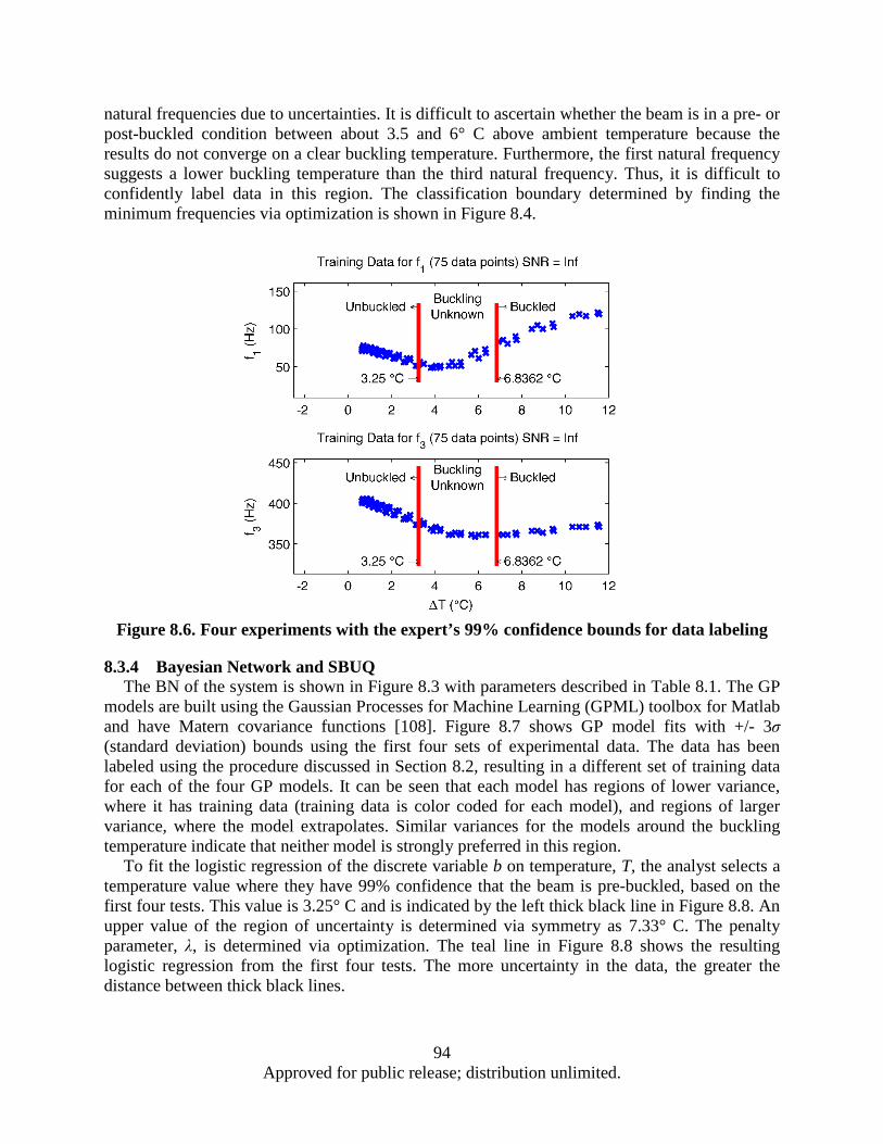
natural frequencies due to uncertainties. It is difficult to ascertain whether the beam is in a pre- or post-buckled condition between about 3.5 and 6° C above ambient temperature because the results do not converge on a clear buckling temperature. Furthermore, the first natural frequency suggests a lower buckling temperature than the third natural frequency. Thus, it is difficult to confidently label data in this region. The classification boundary determined by finding the minimum frequencies via optimization is shown in Figure 8.4.
Figure 8.6. Four experiments with the expert’s 99% confidence bounds for data labeling
8.3.4 Bayesian Network and SBUQ The BN of the system is shown in Figure 8.3 with parameters described in Table 8.1. The GP
models are built using the Gaussian Processes for Machine Learning (GPML) toolbox for Matlab and have Matern covariance functions [108]. Figure 8.7 shows GP model fits with +/- 3σ (standard deviation) bounds using the first four sets of experimental data. The data has been labeled using the procedure discussed in Section 8.2, resulting in a different set of training data for each of the four GP models. It can be seen that each model has regions of lower variance, where it has training data (training data is color coded for each model), and regions of larger variance, where the model extrapolates. Similar variances for the models around the buckling temperature indicate that neither model is strongly preferred in this region.
To fit the logistic regression of the discrete variable b on temperature, T, the analyst selects a temperature value where they have 99% confidence that the beam is pre-buckled, based on the first four tests. This value is 3.25° C and is indicated by the left thick black line in Figure 8.8. An upper value of the region of uncertainty is determined via symmetry as 7.33° C. The penalty parameter, λ, is determined via optimization. The teal line in Figure 8.8 shows the resulting logistic regression from the first four tests. The more uncertainty in the data, the greater the distance between thick black lines.
94 Approved for public release; distribution unlimited.

Figure 8.8. Normal CDFs of original data fitted via least squares. Data points are shown.
Figure 8.7. GP model fits, training data, and 3σ prediction bounds.
95 Approved for public release; distribution unlimited.
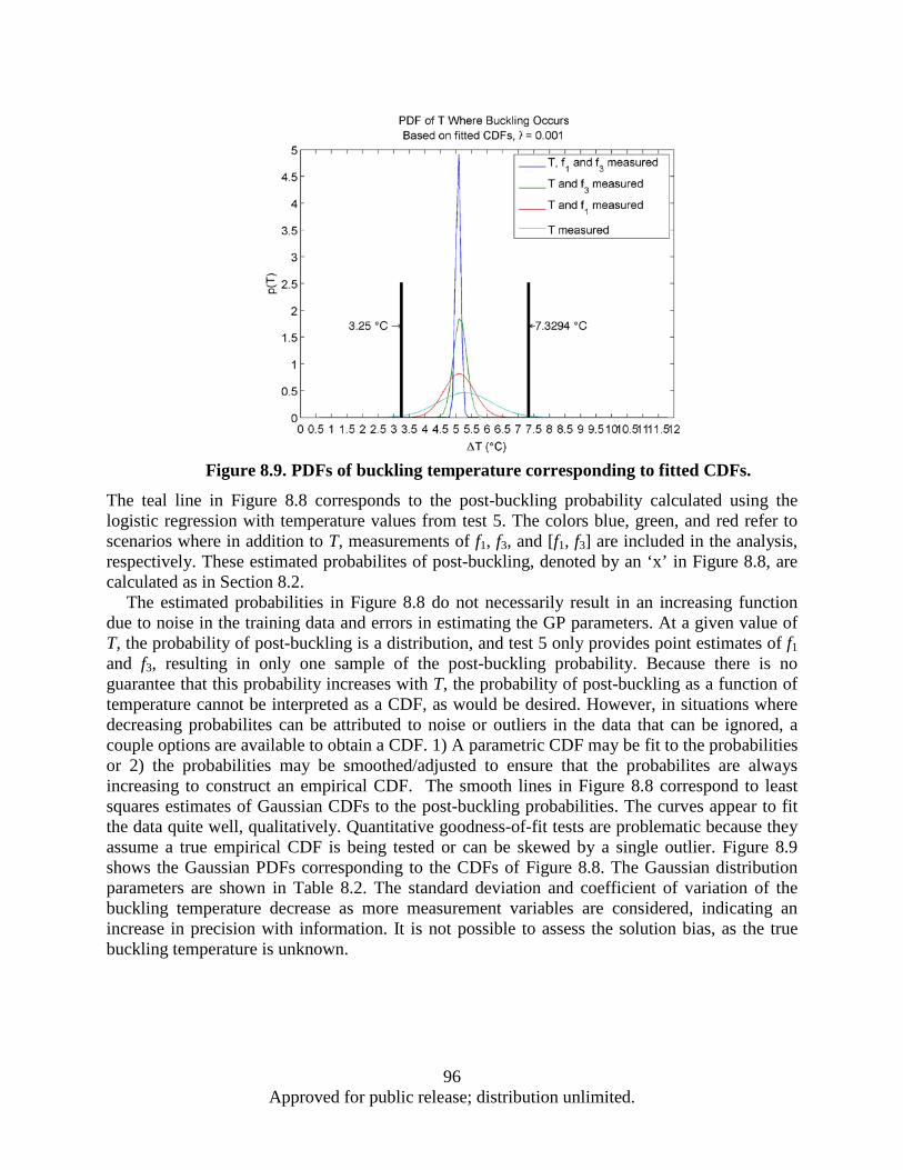
The teal line in Figure 8.8 corresponds to the post-buckling probability calculated using the logistic regression with temperature values from test 5. The colors blue, green, and red refer to scenarios where in addition to T, measurements of f1, f3, and [f1, f3] are included in the analysis, respectively. These estimated probabilites of post-buckling, denoted by an ‘x’ in Figure 8.8, are calculated as in Section 8.2.
The estimated probabilities in Figure 8.8 do not necessarily result in an increasing function due to noise in the training data and errors in estimating the GP parameters. At a given value of T, the probability of post-buckling is a distribution, and test 5 only provides point estimates of f1 and f3, resulting in only one sample of the post-buckling probability. Because there is no guarantee that this probability increases with T, the probability of post-buckling as a function of temperature cannot be interpreted as a CDF, as would be desired. However, in situations where decreasing probabilites can be attributed to noise or outliers in the data that can be ignored, a couple options are available to obtain a CDF. 1) A parametric CDF may be fit to the probabilities or 2) the probabilities may be smoothed/adjusted to ensure that the probabilites are always increasing to construct an empirical CDF. The smooth lines in Figure 8.8 correspond to least squares estimates of Gaussian CDFs to the post-buckling probabilities. The curves appear to fit the data quite well, qualitatively. Quantitative goodness-of-fit tests are problematic because they assume a true empirical CDF is being tested or can be skewed by a single outlier. Figure 8.9 shows the Gaussian PDFs corresponding to the CDFs of Figure 8.8. The Gaussian distribution parameters are shown in Table 8.2. The standard deviation and coefficient of variation of the buckling temperature decrease as more measurement variables are considered, indicating an increase in precision with information. It is not possible to assess the solution bias, as the true buckling temperature is unknown.
Figure 8.9. PDFs of buckling temperature corresponding to fitted CDFs.
96 Approved for public release; distribution unlimited.
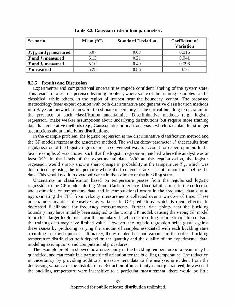
Table 8.2. Gaussian distribution parameters.
Scenario Mean (°C) Standard Deviation Coefficient of Variation
T, f1, and f3 measured 5.07 0.08 0.016 T and f3 measured 5.13 0.21 0.041 T and f1 measured 5.10 0.49 0.096 T measured 5.28 0.86 0.16
8.3.5 Results and Discussion Experimental and computational uncertainties impede confident labeling of the system state.
This results in a semi-supervised learning problem, where some of the training examples can be classified, while others, in the region of interest near the boundary, cannot. The proposed methodology fuses expert opinion with both discriminative and generative classification methods in a Bayesian network framework to estimate uncertainty in the critical buckling temperature in the presence of such classification uncertainties. Discriminative methods (e.g., logistic regression) make weaker assumptions about underlying distributions but require more training data than generative methods (e.g., Gaussian discriminant analysis), which trade data for stronger assumptions about underlying distributions.
In the example problem, the logistic regression is the discriminative classification method and the GP models represent the generative method. The weight decay parameter λ that results from regularization of the logistic regression is a convenient way to account for expert opinion. In the beam example,λ was chosen such that the logistic regression matched where the analyst was at least 99% in the labels of the experimental data. Without this regularization, the logistic regression would simply show a sharp change in probability at the temperature Top, which was determined by using the temperature where the frequencies are at a minimum for labeling the data. This would result in overconfidence in the estimate of the buckling state.
Uncertainty in classification based on temperature passes from the regularized logistic regression to the GP models during Monte Carlo inference. Uncertainties arise in the collection and estimation of temperature data and in computational errors in the frequency data due to approximating the FFT from velocity measurements collected over a window of time. These uncertainties manifest themselves as variance in GP predictions, which is then reflected in decreased likelihoods for frequency measurements. Further, data points near the buckling boundary may have initially been assigned to the wrong GP model, causing the wrong GP model to produce larger likelihoods near the boundary. Likelihoods resulting from extrapolation outside the training data may have limited value. However, the logistic regression helps guard against these issues by producing varying the amount of samples associated with each buckling state according to expert opinion. Ultimately, the estimated bias and variance of the critical buckling temperature distribution both depend on the quantity and the quality of the experimental data, modeling assumptions, and computational procedures.
The example problem showed how uncertainty in the buckling temperature of a beam may be quantified, and can result in a parametric distribution for the buckling temperature. The reduction in uncertainty by providing additional measurement data to the analysis is evident from the decreasing variance of the distributions. Reduction of uncertainty is not guaranteed, however. If the buckling temperature were insensitive to a particular measurement, there would be little
97 Approved for public release; distribution unlimited.
effect on the buckling temperature distribution. Or, a faulty sensor could increase uncertainty in the buckling temperature.
It should be noted that the methodology was demonstrated using particular statistical techniques (logistic regression, Gaussian process models, likelihood weighting inference). However, these need not be the only options. Many other classification techniques could take the place of logistic regression, e.g., support vector machines, neural networks, Gaussian processes. The GP models for the natural frequencies could instead be relevance vector machines or polynomial chaos models or some other response surface method. Likelihood weighting inference could be replace with a Gibbs sampling scheme.
8.4 Summary of State Boundary Uncertainty Quantification The ability to assess uncertainty in state boundaries is of particular importance for complex
systems that have many discrete model choices. This section discussed a methodology for quantifying the uncertainty in a boundary between two system states, namely buckling in a thin beam. First, the system is cast in a Bayesian network framework containing a logistic regression classifier and Gaussian process surrogate models. The BN is trained using data labeled via an optimization procedure. Inference in the Bayesian network is performed using likelihood weighting. Uncertainty in the correct model of the system is quantified over a range of values of a measured variable to obtain the distribution of the state boundary. A Gaussian CDF is fit to the probability of the beam being post-buckled as a function of temperature, and it is seen that the methodology provides more precise estimates as more measurements are made available. The methodology was demonstrated using experimental data from a thin beam experiment.
98 Approved for public release; distribution unlimited.
9 REFERENCES [1] Acar, E., Haftka, R.T., Sankar, B.V., and Qiu, X. (2005). “Increasing design load and
reducing weight of structures by error reduction.” Proc., 46th AIAA/ASME/ASCE/AHS/ASC Structures, Structural Dynamics & Materials Conf., AIAA 2005-2167, Austin, TX.
[2] Tzong, G., Jacobs, R., and Liguore, S. (2010). “Predictive Capability for Hypersonic Structural Response and Life Prediction: Phase 1 - Identification of Knowledge Gaps.” Final Report, AFRL-RB-WP-TR-2010-3068,V1, September 2010.
[3] Zuchowski, B. (2010). “Predictive Capability for Hypersonic Structural Response and Life Prediction: Phase 1 - Identification of Knowledge Gaps.” Final Report, AFRL-RB-WP-TR-2010-3069, August 2010.
[4] McNamara, J.J. and Friedmann, P.P. (2007). “Aeroelastic and aerothermoelastic analysis of hypersonic vehicles: Current status and future trends.” Proc., 48th AIAA/ASME/ASCE/AHS/ASC Structures, Structural Dynamics & Materials Conf., AIAA 2007-2013, Honolulu, HI.
[5] Thornton, E. A. and Dechaumphai, P. (1988). “Coupled flow, thermal, and structural analysis of aerodynamically heated panels.” AIAA J., 25(11), 1052-1059.
[6] Kontinos, D. (1997). “Coupled thermal analysis method with application to metallic thermal protection panels.” J. of Thermophysics and Heat Transfer, 11(2), 173-181.
[7] Blevins, R.D., Bofilios, D., Holehouse, I., Hwa, V.W., Tratt, M.D., Laganelli, A. L., Pozefsky, P., and Pierucci, M. (1989). “Thermo-Vibro-Acoustic Loads and Fatigue of Hypersonic Flight Vehicle Structure - Phase II Report.” Rohr Industries, Inc., RHR 89-202, November 1989.
[8] Blevins, R. D., Holehouse, I., and Wentz, K.R. (1993). “Thermoacoustic loads and fatigue of hypersonic vehicle skin panels.” J. of Aircraft, 30(6), 971-978.
[9] Culler, A.J. and McNamara, J.J. (2010). “Studies on fluid-thermal-structural coupling for aerothermoelasticity in hypersonic flow.” AIAA J., 48(8), 1721-1738.
[10] Culler, A.J. and McNamara, J.J. (2010). “Coupled flow-thermal-structural analysis for response prediction of hypersonic vehicle skin panels.” Proc., 51st AIAA/ASME/ASCE/AHS/ASC Structures, Structural Dynamics & Materials Conf., AIAA 2010-2965, Orlando, FL.
[11] Culler, A.J. and McNamara, J.J. (2011). “Fluid-thermal-structural modeling and analysis of hypersonic structures under combined loading.” Proc., 52nd AIAA/ASME/ASCE/AHS/ASC Structures, Structural Dynamics & Materials Conf., AIAA 2011-1965, Denver, CO.
[12] Falkiewicz, N.J. and Cesnik, C.E.S. (2011). “Enhanced modal solutions for structural dynamics in aerothermoelastic analysis.” Proc., 52nd AIAA/ASME/ASCE/AHS/ASC Structures, Structural Dynamics & Materials Conf., AIAA 2011-1963, Denver, CO.
[13] Lamorte, N., Glaz, B., Friedmann, P.P., Culler, A.J., Crowell, A.R., and McNamara, J.J. (2010). “Uncertainty propagation in hypersonic aerothermoelastic analysis.” Proc., 51st
99 Approved for public release; distribution unlimited.
AIAA/ASME/ASCE/AHS/ASC Structures, Structural Dynamics & Materials Conf., AIAA 2010-2964, Orlando, FL.
[14] Lamorte, N., Friedmann, P.P., Dalle, D.J., Torrez, S.M., and Driscoll, J.F. (2011). “Uncertainty propagation in integrated airframe-propulsion system analysis for hypersonic vehicles.” Proc., 17th AIAA Intl. Space Planes and Hypersonic Systems and Technologies Conf., AIAA 2011-2394, San Francisco, CA.
[15] Ostoich, C., Bodony, D.J., and Geubelle, P.H. (2012). “Fluid-Thermal Response of Spherical Dome Under a Mach 6.59 Boundary Layer.” AIAA J., Vol. 50, No. 12, 2791-2796.
[16] Ostoich, C., Bodony, D.J., and Geubelle, P.H. (2011). “Development and validation of a first principles fluid-thermal multi-physics solver for hypersonic boundary layer heat transfer problems.” Proc., 52nd AIAA/ASME/ASCE/AHS/ASC Structures, Structural Dynamics & Materials Conf., AIAA 2011-1964, Denver, CO.
[17] Rangavajhala, S., Sura, V.S., Hombal, V.K., and Mahadevan, S. (2011). “A new approach to estimate discretization error for multidisciplinary and multidirectional mesh refinement.” Proc., 52nd AIAA/ASME/ASCE/AHS/ASC Structures, Structural Dynamics & Materials Conf., AIAA 2011-1926, Denver, CO.
[18] Rebba, R. and Mahadevan, S. (2006). “Model predictive capability assessment under uncertainty.” AIAA J., 44(10), 2376-2384.
[19] Haldar, A. and Mahadevan, S. (2000). Probability, Reliability and Statistical Methods in Engineering Design, John Wiley & Sons, New York,.
[20] Jensen, F.V., and Jensen, F.B. (2001). Bayesian Networks and Decision Graphs, Springer-Verlag, New York, NY.
[21] Kennedy, M., and O'Hagan, A. (2001). “Bayesian calibration of computer models”. J. of the Royal Statistical Society. Series B (Statistical Methodology), 63(3), 425-464.
[22] Mahadevan, S. (2012). “Uncertainty quantification of system risk assessment and decision-making.” 14th AIAA Non-Deterministic Approaches Conf. Keynote at AIAA SDM 2012, Honolulu, HI.
[23] Smarslok, B.P., Culler, A.J., and Mahadevan, S. (2012). “Error Quantification and Confidence Assessment of Aerothermal Model Predictions for Hypersonic Aircraft.” Proc., 53rd AIAA/ASME/ASCE/AHS/ASC Structures, Structural Dynamics, and Materials Conf., AIAA 2012-1817, Honolulu, HI.
[24] DeCarlo, E.C., Smarslok, B.P., and Mahadevan, S. (2013). “Bayesian Calibration of Aerothermal Models for Hypersonic Air Vehicles.” Proc., 54th AIAA/ASME/ASCE/AHS/ASC Structures, Structural Dynamics, and Materials Conf., AIAA 2013-1683, Boston, MA.
[25] DeCarlo, E.C., Smarslok, B.P., and Mahadevan, S. (2014). “Bayesian Calibration of Coupled Aerothermal Models Using Time-Dependent Data.” Proc., 16th AIAA Non-Deterministic Approaches Conf. at AIAA SciTech 2014, AIAA 2014-0123, National Harbor, MD.
100 Approved for public release; distribution unlimited.
[26] Perez, R., Smarslok, B.P., McNamara, J., and Brouwer, K. (2015). “Investigating Model Uncertainty in the Nonlinear Aeroelastic Response of Thin Panels.” Proc., 17th AIAA Non-Deterministic Approaches Conf. at AIAA SciTech 2015, AIAA 2015-1600, Kissimmee, FL.
[27] Balch, M.S. and Smarslok, B.P. (2014). “A Pre-Validation Study on Supersonic Wind Tunnel Data Collected from Legacy Aerothermal Experiments.” Proc., 16th AIAA Non-Deterministic Approaches Conf. at AIAA SciTech 2014, AIAA 2014-0812, National Harbor, MD.
[28] Bartram, G., Perez, R., Wiebe, R., and Smarslok, B.P. (2015). “Uncertainty Quantification of State Boundaries in Thin Beam Buckling Experiments.” Proc., 17th AIAA Non-Deterministic Approaches Conf. at AIAA SciTech 2015, AIAA 2015-1819, Kissimmee, FL.
[29] Villanueva, D. and Smarslok, B.P. (2015). “Using Expected Information Gain to Design Aerothermal Model Calibration Experiments.” Proc., 17th AIAA Non-Deterministic Approaches Conf. at AIAA SciTech 2015, AIAA 2015-0660, Kissimmee, FL.
[30] Perez, R., Smarslok, B.P., and Mignolet, M. (2015). “Deterministic and Stochastic Partial Linearization Approach for Nonlinear Reduced Order Models of Structures.” Proc., 17th AIAA Non-Deterministic Approaches Conf. at AIAA SciTech 2015, AIAA 2015-2052, Kissimmee, FL.
[31] Smarslok, B.P. and Mahadevan S. (2012). “Investigating Uncertainty in Aerothermal Model Predictions for Hypersonic Aircraft Structures.” Society for Industrial and Applied Mathematics Conf. on Uncertainty Quantification (SIAM UQ12), Raleigh, NC.
[32] Perez, R., Smarslok, B.P., Wang, X.Q., and Mignolet, M.P. (2013). “Investigating Model Uncertainty in Nonlinear Aeroelastic Response of Thin Panels.” 9th Annual Dayton Engineering Sciences Symposium (DESS13), 68, Dayton, OH.
[33] DeCarlo, E.C., Smarslok, B.P., and Mahadevan, S. (2014). “Calibration and Confidence Assessment of Transient, Coupled Models Using Dynamic Bayesian Networks.” Society for Industrial and Applied Mathematics Conf. on Uncertainty Quantification (SIAM UQ14), Savannah, GA.
[34] Smarslok, B.P., DeCarlo, E.C., Perez, R., and Mahadevan, S. (2014). “Identifying Sources of Model Uncertainty in Hypersonic Aerothermoelastic Predictions.” Society for Industrial and Applied Mathematics Conf. on Uncertainty Quantification (SIAM UQ14), Savannah, GA.
[35] Bartram, G., Perez, R., Wiebe, R., and Smarslok, B.P. (2014). “Bayesian Networks for Identification of Thermal Buckling in Thin Beam Experiments.” Society for Industrial and Applied Mathematics Conf. on Uncertainty Quantification (SIAM UQ14), Savannah, GA.
[36] Perez, R., Bartram, G., Wiebe, R., and Smarslok, B.P. (2014). “Bayesian Calibration of Thermal Buckling Models for Thin Panels.” Society for Industrial and Applied Mathematics Conf. on Uncertainty Quantification (SIAM UQ14), Savannah, GA.
101 Approved for public release; distribution unlimited.
[37] Villanueva, D. and Smarslok, B.P. (2014). “Estimating Expected Information Gain for the Design of Calibration Experiments with Multiple Observables.” The Institute for Operations Research and the Management Sciences (INFORMS) Annual Meeting, San Francisco, CA.
[38] Pettit, C. (2008). “Uncertainty Quantification in Aeroelasticity: Recent Results and Research Challenges.” J. of Aircraft, 41(5), 1217-1229.
[39] Weiting, A.R., Dechaumphai, P., Bey, K., Thornton, E.A., and Morgan, K. (1988). “Application of integrated fluid-thermal-structure analysis methods.” NASA TM-100625.
[40] Eason, T.G., Spottswood, S.M., Chona, R., and Penmetsa, R. (2013). “A structures perspective on the challenges associated with analyzing a reusable hypersonic platform.” Proc., 54th AIAA/ASME/ASCE/AHS/ASC Structures, Structural Dynamics & Materials Conf., AIAA 2013-1747, Boston, MA.
[41] Ashley, H., Zartarian, G. (1956). “Piston Theory - A New Aerodynamic Tool for the Aeroelastician.” J. of the Aeronautical Sciences, 23(12), 1109-1118.
[42] Eckert, E.R.G. (1960). “Engineering Relations for Heat Transfer and Friction in High-Velocity Laminar and Turbulent Boundary-Layer Flow over Surfaces with Constant Pressure and Temperature.” Transactions of the ASME, 78(6), 1273-1283.
[43] Matney, A., Perez, R.A., Spottswood, S.M., Wang, X.Q., and Mignolet, M.P. (2012). “Nonlinear structural reduced order modeling methods for hypersonic structures.” Proc., 53rd AIAA/ASME/ASCE/AHS/ASC Structures, Structural Dynamics & Materials Conf., AIAA 2012-1972, Honolulu, HI.
[44] Glass, C.E. and Hunt, L.R. (1986). “Aerothermal Tests of Spherical Dome Protuberances on a Flat Plate at a Mach Number of 6.5.” NASA TP-2631.
[45] Liang, B. and Mahadevan, S. (2011). “Error and uncertainty quantification and sensitivity analysis in mechanics computational models.” Intl. J. for Uncertainty Quantification, 1(2), 147-161.
[46] Deveikis, W.D. and Hunt, L.R. (1973). “Loading and Heating of a Large Flat Plate at Mach 7 in the Langley 8-Foot High-Temperature Structures Tunnel.” NASA TN D-7275.
[47] Liu, Y., Chen, W., Arendt, P., and Huang, H.Z. (2010). “Towards a Better Understanding of Model Validation Metrics.” Proc., 13th AIAA/ISSMO Multidisciplinary Analysis Optimization Conf., AIAA 2010-9240, Fort Worth, TX.
[48] Ling Y. and Mahadevan S. (2012). “Integration of Structural Health Monitoring and Fatigue Damage Prognosis.” Mechanical Systems and Signal Processing, 28, 89-104.
[49] Saltelli, A., Ratto, M., Andres, T. , Campolongo, F., Cariboni, J., Gatelli, D., Saisana, M., and Tarantola, S. (2008). Global sensitivity analysis: the primer. Wiley-Interscience.
[50] Kullback, S., Leibler, R.A. (1951). “On Information and Sufficiency.” Annals of Math. Stat., 22(1), 79-86.
[51] Rebba, A., Mahadevan, S. (2008). “Computational Methods for Model Reliability Assessment.” Reliability Engineering & System Safety, 93(8), 1197-1207.
102 Approved for public release; distribution unlimited.
[52] Lamorte, N., Friedmann, P.P., Glaz, B., Culler, A.J., Crowell, A.R., and McNamara, J.J. (2014). “Uncertainty Propagation in Hypersonic Aerothermoelastic Analysis.” J. of Aircraft, 51(1), 192-203.
[53] Skujins, T. (2013). Reduced-Order Modeling of Unsteady Aerodynamics Across Multiple Mach Regimes, Ph.D. Thesis, University of Michigan, Ann Arbor.
[54] Lighthill, M.J. (1953). “Oscillating Airfoils at High Mach Numbers.” J. of the Aeronautical Sciences, 20(6).
[55] Crowell, A.R., McNamara, J.J., and Miller, B.A. (2011). “Hypersonic Aeroelastic Response Prediction of Skin Panels Using Computational Fluid Dynamic Surrogates.” ASD J., 2(2), 3-30.
[56] McNamara, J.J., Crowell, A. R., Friedmann, P.P., Glaz, B., and Gogulapti A. (2010). “Approximate Modeling of Unsteady Aerodynamics for Hypersonic Aeroelasticity.” J. of Aircraft, 47(6), 1932-1945.
[57] Liu, D. D., Yao, Z. X., Sarhaddi, D., and Chavez, F. (1997). “From Piston Theory to a Unified Hypersonic-Supersonic Lifting Surface Method.” J. of Aircraft, 34(3), 304-312.
[58] Moser B. and Oliver T. (2013). “Representing Uncertainty due to Inaccurate Models.” Workshop on Large Scale Inverse Problems and Quantification of Uncertainty: Big Data Meets Big Models, Santa Fe, NM.
[59] March, A. and Willcox, K., (2012). “Provably Convergent Multifidelity Optimization Algorithm Not Requiring High-Fidelity Derivatives.” AIAA J., 50(5), 1079-1089.
[60] Fung, Y.C., and Tong, T. (2001). Classical and Computational Solid Mechanics, World Scientific, River Edge, NJ.
[61] Bonet, J., and Wood, R.D. (1997). Nonlinear Continuum Mechanics for Finite Element Analysis, Cambridge University Press, Cambridge.
[62] Kim, K., Radu, A.G., Wang, X.Q., and Mignolet, M.P. (2013). “Nonlinear Reduced Order Modeling of Isotropic and Functionally Graded Plates.” Intl. J. of Nonlinear Mechanics, 49, 100-110.
[63] Hollkamp, J.J. and Gordon, R.W. (2005). “Modeling Membrane Displacements in the Sonic Fatigue Response Prediction Problem.” Proc., 46th AIAA/ASME/ASCE/AHS/ASC Structures, Structural Dynamics & Materials Conf., AIAA 2005-2095, Austin, TX.
[64] Nydick, I., Friedmann, P.P., and Zhong, X. (1995). “Hypersonic Panel Flutter Studies on Curved Panels.” Proc. 36th AIAA/ASME/ASCE/AHS/ASC Structures, Structural Dynamics and Materials Conf., AIAA 1995-1485, New Orleans, LA.
[65] McNamara, J. (2005). Aeroelastic and Aerothermoelastic Behavior of Two and Three Dimensional Surfaces in Hypersonic Flow, Ph.D. Thesis, University of Michigan, Ann Arbor.
[66] S. N. Lophaven, H. B. Nielsen, and J. Sondergaard. (2002). DACE A Matlab Kriging Toolbox Version 2.0. Technical Report IMM-TR-2002-12.
103 Approved for public release; distribution unlimited.
[67] Saltelli, A., Annoni, P., Azzini, I., Compolongo, F., Ratto, M., and Tarantola, S. (2010). “Variance based sensitivity analysis of model output. Design and estimator for the total sensitivity index.” Computer Physics Communications, 181, 259-270.
[68] Sobol’, I.M. (1967). “On the distribution of points in a cube and the approximate evaluation of integrals.” USSR Comput. Maths. Math. Phys., 7, 86-112.
[69] Sobol’, I.M. (1976). “Uniformly distributed sequences with an addition uniform property.” USSR Comput. Maths. Math. Phys., 16, 236-242.
[70] Ferson, S., Oberkampf, W. L., and Ginzburg, L. (2008). “Model validation and predictive capability for the thermal challenge problem.” Computer Methods in Applied Mechanics and Engineering , 197(29), 2408-2430.
[71] Balch, M. S. (2012). “Mathematical Foundations for a Theory of Confidence Structures.” Intl. J. of Approximate Reasoning , 53, 2012, 1003-1019.
[72] Anderson, Jr., J. D. (2003). Modern Compressible Flow with Historical Perspective, 3rd Ed., McGraw-Hill, New York.
[73] Posada, D., and Buckley, T. R. (2004). “Model Selection and Model Averaging in Phylogenetics: Advantages of Akaike Information Criterion and Bayesian Approaches Over Likelihood Ratio Tests.” Systematic Biology, 53, 793-808.
[74] Raftery, A. (1995). “Bayesian Model Selection in Social Research.” Sociological Methodology, 25, 111-163.
[75] Johnson, J. B., and Omland, K. S. (2004). “Model selection in ecology and evolution.” Trends in Ecology & Evolution, 19, 101-108.
[76] Abascal, F., Zardoya, R., and Posada, D. (2005). “ProtTest: selection of best-fit models of protein evolution.” Bioinformatics, 21, 2104-2105.
[77] Zaki, M.J., Hsiao, C.J. (2002). “CHARM: An efficient algorithm for closed itemset mining.” Proc., SIAM Intl. Conf. on Data Mining, Philadelphia, PA.
[78] Neyman, J., and Pearson, E. S. (1933). “On the Problem of the Most Efficient Tests of Statistical Hypotheses.” Philosophical Transactions of the Royal Society of London. Series A, Containing Papers of a Mathematical or Physical Character, 231, 289-337.
[79] Akaike, H. (1974). “A new look at the statistical model identification.” IEEE Transactions on Automatic Control, 19, 716-723.
[80] Murata, N., Yoshizawa, S., and Amari, S.-I. (1994). “Network information criterion-determining the number of hidden units for an artificial neural network model.” IEEE Transactions on Neural Networks, 5, 865-872.
[81] Sugiura, N. (1978). “Further analysts of the data by akaike’ s information criterion and the finite corrections.” Communications in Statistics - Theory and Methods, 7, 13-26.
[82] Claeskens, G., and Hjort, N. L. (2003). “The Focused Information Criterion.” J. of the American Statistical Association, 98, 900-916.
[83] Vuong, Q. H. (1989). “Likelihood Ratio Tests for Model Selection and Non-Nested Hypotheses.” Econometrica, 57, 307-333.
104 Approved for public release; distribution unlimited.
[84] Burnham, K. P., and Anderson, D. R. (2004). “Multimodel Inference Understanding AIC and BIC in Model Selection.” Sociological Methods & Research, 33, 261-304.
[85] Bouckaert, R. R. (1993). “Probabilistic Network Construction Using the Minimum Description Length Principle.” Symbolic and Quantitative Approaches to Reasoning and Uncertainty - Lecture Notes in Computer Science, 747, 41-48.
[86] Spiegelhalter, D. J., Best, N. G., Carlin, B. P., and Van Der Linde, A. (2002). “Bayesian measures of model complexity and fit.” J. of the Royal Statistical Society: Series B (Statistical Methodology), 64, 583-639.
[87] Schwarz, G. (1978). “Estimating the Dimension of a Model.” The Annals of Statistics, 6, 461-464.
[88] Kass, R. E., and Raftery, A. E. (1995). “Bayes Factors.” J. of the American Statistical Association, 90, 773-795.
[89] Smith, A. F. M., and Spiegelhalter, D. J. (1980). “Bayes Factors and Choice Criteria for Linear Models.” J. of the Royal Statistical Society. Series B (Methodological), 42, 213-220.
[90] Jeffreys, H. (1998). Theory of probability, Oxford University Press US.
[91] Madigan, D., and Raftery, A. E. (1994). “Model Selection and Accounting for Model Uncertainty in Graphical Models Using Occam’s Window.” J. of the American Statistical Association, 89, 1535-1546.
[92] Hoeting, J. A., Madigan, D., Raftery, A. E., and Volinsky, C. T. (1999). “Bayesian Model Averaging: A Tutorial.” Statistical Science, 14, 382-401.
[93] Carlin, B. P., and Chib, S. (1992). “Bayesian model choice via Markov chain Monte Carlo methods.” J. of the Royal Statistical Society. Series B (Methodological), 57, 473-484.
[94] Green, P. J. (1995). “Reversible Jump Markov Chain Monte Carlo Computation and Bayesian Model Determination.” Biometrika, 82, 711-732.
[95] Koller, D., and Friedman, N. (2009). Probabilistic Graphical Models: Principles and Techniques, MIT Press, Cambridge.
[96] Frieden, B. R. (2004). Science from Fisher Information: A Unification, Cambridge University Press, Cambridge.
[97] Zhang, T., and Oles, F. (2000). “The value of unlabeled data for classification problems.” Proc., of the Seventeenth Intl. Conf. on Machine Learning, 1191-1198.
[98] Hombal, V. K., and Mahadevan, S. (2013). “Model Selection Among Physics-Based Models.” J. of Mechanical Design, 135(2).
[99] Jr, D. W. H., and Lemeshow, S. (2004). Applied Logistic Regression, John Wiley & Sons.
[100] Hopfield, J. J. (1982). “Neural networks and physical systems with emergent collective computational abilities..” Proc., National Academy of Sciences of the United States of America, 79, 2554-2558.
105 Approved for public release; distribution unlimited.

[101] Burges, C. J. C. (1998). “A Tutorial on Support Vector Machines for Pattern Recognition.” Data Mining and Knowledge Discovery, 2, 121-167.
[102] Tipping, M. E. (2001). “Sparse Bayesian learning and the relevance vector machine.” J. of Machine Learning Research, 1, 211-244.
[103] Fraley, C., and Raftery, A. E. (2002). “Model-based clustering, discriminant analysis, and density estimation.” J. of the American Statistical Association, 611-631.
[104] Shukla, A., and Mignolet, M., “Identification and Updating of Uncertain Dynamic Models of a Flat Beam for Nonlinear Forced Response Predictions.” Proc. 52nd AIAA/ASME/ASCE/AHS/ASC Structures, Structural Dynamics and Materials Conf., Denver, CO: American Institute of Aeronautics and Astronautics, 2011.
[105] Kosmatka, J., “Damping in Initially Stressed Elastically Unstable Structures.” Proc., 50th AIAA/ASME/ASCE/AHS/ASC Structures, Structural Dynamics, and Materials Conf., American Institute of Aeronautics and Astronautics,.
[106] Tikhonov, A. (1963). “Solution of incorrectly formulated problems and the regularization method.” Soviet Math. Dokl., 1035-1038.
[107] Hoerl, A. E., and Kennard, R. W. (1970). “Ridge Regression: Biased Estimation for Nonorthogonal Problems.” Technometrics, 12, 55-67.
[108] Rasmussen, C. E. and Nickisch, H. (2010). “Gaussian processes for machine learning (GPML) toolbox.” J. of Machine Learning Research, 11, 3011-3015.
106 Approved for public release; distribution unlimited.