Embed Size (px)
Citation preview
QUANTIFYING THE PERFORMANCE OF
NATURAL VENTILATION WINDCATCHERS
A thesis submitted for the degree of Doctor of Environmental
Technology
by
BENJAMIN MICHAEL JONES
School of Engineering and Design
Brunel University
July 2010
ABSTRACT i
Abstract
The significant energy consumption of non-domestic buildings has led to renewed interest in
natural ventilation strategies that utilise the action of the wind, and the buoyancy of hot air.
One natural ventilation element is the Windcatcher, a roof mounted device that works by
channelling air into a room under the action of wind pressure, whilst simultaneously drawing
air out of the room by virtue of a low pressure region created downstream of the element. A
significant number of Windcatchers are fitted in UK schools where good indoor air quality is
essential for the health and performance of children. The performance of a ventilation system
in a school classroom is determined by its ability to provide ventilation in accordance with
UK government ventilation, air quality, and acoustic requirements. However, there is only
limited performance data available for a Windcatcher, particularly when operating in–situ.
Accordingly, this thesis investigates the performance of a Windcatcher in three ways: First,
a semi-empirical model is developed that combines an envelope flow model with existing
experimental data. Second, measurements of air temperature, relative humidity, carbon
dioxide, and noise levels in school classrooms are assessed over summer and winter months
and the results compared against UK Government requirements. Finally, air flow rates are
measured in twenty four classrooms and compared against the semi-empirical predictions.
The monitoring reveals that air quality in classrooms ventilated by a Windcatcher has the
potential to be better than that reported for conventional natural ventilation strategies such
as windows. Furthermore, an autonomous Windcatcher is shown to deliver the minimum
ventilation rates specified by the UK Government, and when combined with open windows
a Windcatcher is also capable of providing the required mean and purge ventilation rates.
These findings are then used to develop an algorithm that will size a Windcatcher for a
particular application, as well as helping to improve the ventilation strategy for a building
that employs a Windcatcher.
CONTENTS ii
Contents
Abstract i
List of Figures vii
List of Tables xiv
Nomenclature xvi
Executive Summary 1
1 Introduction 12
1.1 The Environment . . . . . . . . . . . . . . . . . . . . . . . . . . . . . . . . . . 12
1.2 The Indoor Environment . . . . . . . . . . . . . . . . . . . . . . . . . . . . . . 13
1.3 Naturally Ventilated Buildings . . . . . . . . . . . . . . . . . . . . . . . . . . 15
1.4 School Buildings . . . . . . . . . . . . . . . . . . . . . . . . . . . . . . . . . . 22
1.5 Research Aim and Objectives . . . . . . . . . . . . . . . . . . . . . . . . . . . 24
1.6 Thesis Outline . . . . . . . . . . . . . . . . . . . . . . . . . . . . . . . . . . . 25
2 Literature Review 27
2.1 Indoor Environment Quality and Ventilation . . . . . . . . . . . . . . . . . . 27
2.1.1 Thermal Comfort and Ventilation . . . . . . . . . . . . . . . . . . . . 29
2.1.2 Indoor Air Quality and Ventilation . . . . . . . . . . . . . . . . . . . . 34
2.1.3 Indoor Air Quality and Ventilation in Schools . . . . . . . . . . . . . . 40
2.1.4 Indoor Environmental Noise and Ventilation . . . . . . . . . . . . . . . 51
2.2 The Measurement and Prediction of Natural Ventilation . . . . . . . . . . . . 54
CONTENTS iii
2.2.1 Predicting Natural Ventilation Performance . . . . . . . . . . . . . . . 54
2.2.2 Measuring Natural Ventilation Performance . . . . . . . . . . . . . . . 58
2.3 Measurement and Prediction of Air Flow Through a
Windcatcher . . . . . . . . . . . . . . . . . . . . . . . . . . . . . . . . . . . . 60
2.3.1 Quantifying the Performance of Vernacular Wind–Catchers . . . . . . 61
2.3.2 Theoretical and Experimental Investigations of a Windcatcher . . . . 63
2.3.3 Investigations of a Windcatcher In–Situ . . . . . . . . . . . . . . . . . 69
2.4 Conclusions . . . . . . . . . . . . . . . . . . . . . . . . . . . . . . . . . . . . . 70
3 Theory: Modelling Flow Through a Windcatcher System 72
3.1 Analytic Model . . . . . . . . . . . . . . . . . . . . . . . . . . . . . . . . . . . 73
3.1.1 Sealed Room Ventilated by an Autonomous Windcatcher . . . . . . . 79
3.1.2 Unsealed Room Ventilated by an Autonomous Windcatcher . . . . . . 84
3.1.3 Room Ventilated by a Windcatcher in Coordination with a Facade
Opening . . . . . . . . . . . . . . . . . . . . . . . . . . . . . . . . . . . 88
3.2 Semi–Empirical Model . . . . . . . . . . . . . . . . . . . . . . . . . . . . . . . 102
3.2.1 Autonomous Windcatcher . . . . . . . . . . . . . . . . . . . . . . . . . 103
3.2.2 Determining Pressure Loss Coefficients . . . . . . . . . . . . . . . . . . 105
3.2.3 Identification of Component Losses . . . . . . . . . . . . . . . . . . . . 110
3.2.4 Corroborating the Predictions for an Autonomous Windcatcher . . . . 112
3.2.5 Simplifying the Semi–Empirical Model . . . . . . . . . . . . . . . . . . 116
3.2.6 Windcatcher with Facade Opening . . . . . . . . . . . . . . . . . . . . 118
3.2.7 Comparing the Performance of Windcatcher Systems . . . . . . . . . . 123
3.3 Summary . . . . . . . . . . . . . . . . . . . . . . . . . . . . . . . . . . . . . . 126
4 Case Studies 128
4.1 School Buildings . . . . . . . . . . . . . . . . . . . . . . . . . . . . . . . . . . 128
4.1.1 School C . . . . . . . . . . . . . . . . . . . . . . . . . . . . . . . . . . 130
4.1.2 School D . . . . . . . . . . . . . . . . . . . . . . . . . . . . . . . . . . 131
4.1.3 School E . . . . . . . . . . . . . . . . . . . . . . . . . . . . . . . . . . . 132
4.1.4 School F . . . . . . . . . . . . . . . . . . . . . . . . . . . . . . . . . . . 133
4.1.5 School G . . . . . . . . . . . . . . . . . . . . . . . . . . . . . . . . . . 134
CONTENTS iv
4.1.6 School H . . . . . . . . . . . . . . . . . . . . . . . . . . . . . . . . . . 135
4.1.7 School I . . . . . . . . . . . . . . . . . . . . . . . . . . . . . . . . . . . 136
4.1.8 Environmental Conditions . . . . . . . . . . . . . . . . . . . . . . . . . 137
4.2 School Classrooms . . . . . . . . . . . . . . . . . . . . . . . . . . . . . . . . . 139
4.3 Ventilation Strategy and Control . . . . . . . . . . . . . . . . . . . . . . . . . 143
4.4 Measuring Indoor Environment Quality . . . . . . . . . . . . . . . . . . . . . 147
4.4.1 Indoor Air Quality . . . . . . . . . . . . . . . . . . . . . . . . . . . . . 147
4.4.2 Ventilation Rate . . . . . . . . . . . . . . . . . . . . . . . . . . . . . . 152
4.4.3 Noise . . . . . . . . . . . . . . . . . . . . . . . . . . . . . . . . . . . . 155
4.5 Summary . . . . . . . . . . . . . . . . . . . . . . . . . . . . . . . . . . . . . . 155
5 Results: IEQ in Case Study Classrooms 157
5.1 Indoor Air Quality . . . . . . . . . . . . . . . . . . . . . . . . . . . . . . . . . 157
5.1.1 Temperature . . . . . . . . . . . . . . . . . . . . . . . . . . . . . . . . 158
5.1.2 Carbon Dioxide . . . . . . . . . . . . . . . . . . . . . . . . . . . . . . . 161
5.1.3 Relative Humidity . . . . . . . . . . . . . . . . . . . . . . . . . . . . . 165
5.2 Ventilation . . . . . . . . . . . . . . . . . . . . . . . . . . . . . . . . . . . . . 166
5.3 Ambient Noise . . . . . . . . . . . . . . . . . . . . . . . . . . . . . . . . . . . 175
5.4 Night Cooling . . . . . . . . . . . . . . . . . . . . . . . . . . . . . . . . . . . . 178
5.5 Summary . . . . . . . . . . . . . . . . . . . . . . . . . . . . . . . . . . . . . . 182
6 Results: A Comparison Between Predicted and Measured Ventilation Rates 184
6.1 Autonomous Windcatcher . . . . . . . . . . . . . . . . . . . . . . . . . . . . . 186
6.2 Windcatcher in Coordination with Open Windows . . . . . . . . . . . . . . . 191
6.3 Application of the Semi–Empirical Model to Windcatcher Design . . . . . . . 195
6.3.1 Design Steps . . . . . . . . . . . . . . . . . . . . . . . . . . . . . . . . 205
6.4 Summary . . . . . . . . . . . . . . . . . . . . . . . . . . . . . . . . . . . . . . 212
7 Discussion of results 214
7.1 Providing Thermal Comfort and Air Quality . . . . . . . . . . . . . . . . . . 214
7.1.1 Demand Control Ventilation . . . . . . . . . . . . . . . . . . . . . . . . 216
7.1.2 Dynamic Comfort Control . . . . . . . . . . . . . . . . . . . . . . . . . 222
CONTENTS v
7.2 Providing Efficient Ventilation Flow Paths . . . . . . . . . . . . . . . . . . . . 231
7.3 Improving the Windcatcher System . . . . . . . . . . . . . . . . . . . . . . . . 236
7.4 Application of the Windcatcher to Other Non–Domestic Building Types . . . 238
7.5 Immediate Application of this Work . . . . . . . . . . . . . . . . . . . . . . . 240
8 Conclusions 243
9 Further Work 246
References 249
Appendices 268
A Predicting Ventilation Rates Through a Room Ventilated by a Windcatcher
in Coordination with a Facade Opening. 268
B Case Study Details 271
B.1 School C . . . . . . . . . . . . . . . . . . . . . . . . . . . . . . . . . . . . . . . 272
B.2 School D . . . . . . . . . . . . . . . . . . . . . . . . . . . . . . . . . . . . . . . 274
B.3 School E . . . . . . . . . . . . . . . . . . . . . . . . . . . . . . . . . . . . . . . 275
B.4 School F . . . . . . . . . . . . . . . . . . . . . . . . . . . . . . . . . . . . . . . 276
B.5 School G . . . . . . . . . . . . . . . . . . . . . . . . . . . . . . . . . . . . . . . 277
B.6 School H . . . . . . . . . . . . . . . . . . . . . . . . . . . . . . . . . . . . . . . 278
B.7 School I . . . . . . . . . . . . . . . . . . . . . . . . . . . . . . . . . . . . . . . 280
C Indoor Air Quality 282
C.1 Temperature . . . . . . . . . . . . . . . . . . . . . . . . . . . . . . . . . . . . 282
C.2 Carbon Dioxide . . . . . . . . . . . . . . . . . . . . . . . . . . . . . . . . . . . 285
C.3 Relative Humidity . . . . . . . . . . . . . . . . . . . . . . . . . . . . . . . . . 286
D Ventilation Rates 287
E Sound Pressure Levels 293

CONTENTS vi
F Published Literature 295
FIGURES vii
List of Figures
0 Competing concerns for the Research Engineer. . . . . . . . . . . . . . . . . . 2
1.1 The Monodraught Windcatcher. . . . . . . . . . . . . . . . . . . . . . . . . . 21
2.1 Single sided ventilation, single opening. . . . . . . . . . . . . . . . . . . . . . 48
2.2 Single sided ventilation, double opening. . . . . . . . . . . . . . . . . . . . . . 48
2.3 Cross ventilation, facade opening. . . . . . . . . . . . . . . . . . . . . . . . . . 49
2.4 Cross ventilation, facade opening and clerestory windows. . . . . . . . . . . . 49
2.5 Stack ventilation. . . . . . . . . . . . . . . . . . . . . . . . . . . . . . . . . . . 49
2.6 Stack ventilation, corridor and/or atrium. . . . . . . . . . . . . . . . . . . . . 49
2.7 Top down ventilation, wind–catcher. . . . . . . . . . . . . . . . . . . . . . . . 50
2.8 Top down ventilation, wind–catcher with facade opening. . . . . . . . . . . . 50
3.1 Plan view of Windcatcher. . . . . . . . . . . . . . . . . . . . . . . . . . . . . . 73
3.2 Side view of Windcatcher. . . . . . . . . . . . . . . . . . . . . . . . . . . . . . 73
3.3 Primary flow paths for a sealed room ventilated by an autonomous Wind-
catcher with wind incident at θ = 0◦. . . . . . . . . . . . . . . . . . . . . . . . 79
3.4 Primary flow paths for a sealed room ventilated by an autonomous Wind-
catcher with wind incident at θ = 45◦. . . . . . . . . . . . . . . . . . . . . . . 82
3.5 Secondary flow paths for a sealed room ventilated by an autonomous Wind-
catcher with wind incident at θ = 45◦ and TE > TI . . . . . . . . . . . . . . . . 82
3.6 Primary flow paths for an unsealed room ventilated by an autonomous Wind-
catcher with wind incident at θ = 0◦. . . . . . . . . . . . . . . . . . . . . . . . 84
3.7 Secondary flow paths for an unsealed room ventilated by an autonomous Wind-
catcher with wind incident at θ = 0◦ and TI > TE . . . . . . . . . . . . . . . . 85
FIGURES viii
3.8 Secondary flow paths for an unsealed room ventilated by an autonomous Wind-
catcher with wind incident at θ = 0◦ and TE > TI . . . . . . . . . . . . . . . . 85
3.9 Primary flow paths for an unsealed room ventilated by an autonomous Wind-
catcher with wind incident at θ = 45◦. . . . . . . . . . . . . . . . . . . . . . . 86
3.10 Secondary flow paths for an unsealed room ventilated by an autonomous Wind-
catcher with wind incident at θ = 45◦ and TI > TE . . . . . . . . . . . . . . . . 87
3.11 Secondary flow paths for an unsealed room ventilated by an autonomous Wind-
catcher with wind incident at θ = 45◦ and TE > TI . . . . . . . . . . . . . . . . 87
3.12 Primary flow paths for a room ventilated by a Windcatcher with wind incident
at θ = 0◦, and a facade opening with Cp5 > 0. . . . . . . . . . . . . . . . . . . 89
3.13 Secondary flow paths for a room ventilated by a Windcatcher with wind inci-
dent at θ = 0◦, and a facade opening with Cp5 > 0. . . . . . . . . . . . . . . . 89
3.14 Primary flow paths for a room ventilated by a Windcatcher with wind incident
at θ = 0◦, and a facade opening with Cp5 < 0. . . . . . . . . . . . . . . . . . . 93
3.15 Secondary flow paths for a room ventilated by a Windcatcher with wind inci-
dent at θ = 0◦, and a facade opening with Cp5 < 0. . . . . . . . . . . . . . . . 93
3.16 Primary flow paths for a room ventilated by a Windcatcher with wind incident
at θ = 45◦, and a facade opening with Cp5 > 0. . . . . . . . . . . . . . . . . . 97
3.17 Secondary flow paths for a room ventilated by a Windcatcher with wind inci-
dent at θ = 45◦, and a facade opening with Cp5 > 0. . . . . . . . . . . . . . . 97
3.18 Primary flow paths for a room ventilated by a Windcatcher with wind incident
at θ = 45◦, and a facade opening with Cp5 < 0. . . . . . . . . . . . . . . . . . 99
3.19 Secondary flow paths for a room ventilated by a Windcatcher with wind inci-
dent at θ = 45◦, and a facade opening with Cp5 < 0. . . . . . . . . . . . . . . 99
3.20 Comparison between semi–empirical predictions and the experimental mea-
surements of Elmualim & Awbi (2002a) without dampers and grill for θ = 0◦. 105
3.21 Predicted Reynolds Number in Windcatcher quadrants. . . . . . . . . . . . . 105
3.22 Predicted pressure in a sealed room without dampers and grill for θ = 0◦. . . 107
3.23 Comparison between semi–empirical predictions and the experimental mea-
surements of Elmualim (2005a) with dampers and grill for θ = 0◦. . . . . . . 107
3.24 Change of Kinetic Energy Coefficient with Reynolds Number. . . . . . . . . . 109
FIGURES ix
3.25 Comparison between semi–empirical predictions with and without the Kinetic
Energy Coefficient. . . . . . . . . . . . . . . . . . . . . . . . . . . . . . . . . . 109
3.26 Measurements by Parker & Teekeram (2004b) of flow rate into and out of the
top section of a Windcatcher. . . . . . . . . . . . . . . . . . . . . . . . . . . . 110
3.27 Comparison between semi–empirical predictions and the CFD predictions of
Li & Mak (2007) for ventilation rates from a sealed room, without dampers
and grill. . . . . . . . . . . . . . . . . . . . . . . . . . . . . . . . . . . . . . . . 113
3.28 Comparison between semi–empirical predictions and the experimental mea-
surements Elmualim & Teekaram (2002) for ventilation rates in each quadrant
when ventilating a sealed room, without dampers and grill. . . . . . . . . . . 113
3.29 Comparison between semi–empirical predictions and the experimental mea-
surements of Elmualim (2005b) without dampers and grill for θ = 0◦. . . . . . 114
3.30 Predicted pressure in a sealed room. . . . . . . . . . . . . . . . . . . . . . . . 114
3.31 Predictions for an unsealed room when θ = 0◦. . . . . . . . . . . . . . . . . . 114
3.32 Predictions for an unsealed room when θ = 45◦. . . . . . . . . . . . . . . . . . 114
3.33 Prediction of the effect of the area of a shielded facade opening on Windcatcher
ventilation rates. . . . . . . . . . . . . . . . . . . . . . . . . . . . . . . . . . . 120
3.34 Prediction of ventilation rates for a 1000 mm Windcatcher with A5 = 1 m2 and
θ = 45◦. . . . . . . . . . . . . . . . . . . . . . . . . . . . . . . . . . . . . . . . 122
3.35 Prediction of ventilation rate from a room with varying Cp5 for the facade
opening. . . . . . . . . . . . . . . . . . . . . . . . . . . . . . . . . . . . . . . . 123
3.36 Prediction of the effect of the area of an exposed facade opening on Wind-
catcher ventilation rates. . . . . . . . . . . . . . . . . . . . . . . . . . . . . . . 123
3.37 Prediction of the effect of a shielded trickle vent opening on Windcatcher
ventilation rates. . . . . . . . . . . . . . . . . . . . . . . . . . . . . . . . . . . 125
3.38 Prediction of the effect of an exposed trickle vent opening on Windcatcher
ventilation rates. . . . . . . . . . . . . . . . . . . . . . . . . . . . . . . . . . . 125
4.1 School C, aerial view. . . . . . . . . . . . . . . . . . . . . . . . . . . . . . . . 130
4.2 School D, aerial view. . . . . . . . . . . . . . . . . . . . . . . . . . . . . . . . 131
4.3 School E, aerial view. . . . . . . . . . . . . . . . . . . . . . . . . . . . . . . . 132
FIGURES x
4.4 School F, aerial view. . . . . . . . . . . . . . . . . . . . . . . . . . . . . . . . . 133
4.5 School G, aerial view. . . . . . . . . . . . . . . . . . . . . . . . . . . . . . . . 134
4.6 School H, aerial view. . . . . . . . . . . . . . . . . . . . . . . . . . . . . . . . 135
4.7 School I, aerial view. . . . . . . . . . . . . . . . . . . . . . . . . . . . . . . . . 136
4.8 External temperature for the south east of England. . . . . . . . . . . . . . . 137
4.9 External temperature for the south west of England. . . . . . . . . . . . . . . 137
4.10 Wind speed for the south east of England. . . . . . . . . . . . . . . . . . . . . 138
4.11 Wind speed for the south west of England. . . . . . . . . . . . . . . . . . . . 138
4.12 Frequency of wind direction for the south east of England. . . . . . . . . . . . 139
4.13 Frequency of wind direction for the south west of England. . . . . . . . . . . 139
4.14 Ventilation strategy, school C. . . . . . . . . . . . . . . . . . . . . . . . . . . . 145
4.15 Ventilation strategy, school D. . . . . . . . . . . . . . . . . . . . . . . . . . . . 145
4.16 Ventilation strategy, school E. . . . . . . . . . . . . . . . . . . . . . . . . . . . 145
4.17 Ventilation strategy, school F. . . . . . . . . . . . . . . . . . . . . . . . . . . . 145
4.18 Ventilation strategy, school G. . . . . . . . . . . . . . . . . . . . . . . . . . . . 145
4.19 Ventilation strategy, school H. . . . . . . . . . . . . . . . . . . . . . . . . . . . 145
4.20 Ventilation strategy, school I. . . . . . . . . . . . . . . . . . . . . . . . . . . . 146
4.21 Floor transition, cross–section view. . . . . . . . . . . . . . . . . . . . . . . . 146
4.22 Example of CO2 concentration in a classroom. . . . . . . . . . . . . . . . . . 150
4.23 Example of air temperature in a classroom. . . . . . . . . . . . . . . . . . . . 151
4.24 Example of relative humidity in a classroom. . . . . . . . . . . . . . . . . . . 151
4.25 Example of the tracer gas decay method. . . . . . . . . . . . . . . . . . . . . 153
5.1 Measured air temperature for occupied hours in summer. . . . . . . . . . . . 158
5.2 Measured air temperature for occupied hours in winter. . . . . . . . . . . . . 158
5.3 Difference between measured mean internal and external temperatures (∆T )
for occupied hours in summer. . . . . . . . . . . . . . . . . . . . . . . . . . . . 159
5.4 Frequency of Windcatcher damper position during occupied hours. . . . . . . 160
5.5 Measured CO2 for occupied hours in summer. . . . . . . . . . . . . . . . . . . 162
5.6 Measured CO2 for occupied hours in winter. . . . . . . . . . . . . . . . . . . . 162
FIGURES xi
5.7 Cumulative frequency of mean carbon dioxide levels in mechanically and nat-
urally ventilated school classrooms during occupied hours. . . . . . . . . . . . 165
5.8 Measured relative humidity for occupied hours in summer. . . . . . . . . . . . 166
5.9 Measured relative humidity for occupied hours in winter. . . . . . . . . . . . . 166
5.10 Estimated ventilation rate per person: Windcatcher closed and windows closed.173
5.11 Estimated ventilation rate per person: Windcatcher open and windows closed. 173
5.12 Estimated ventilation rate per person: Windcatcher open and windows open. 174
5.13 Estimated ventilation rate per person: Windcatcher closed and windows open. 174
5.14 Cumulative frequency of mean flow rates in school classrooms during occupied
hours. . . . . . . . . . . . . . . . . . . . . . . . . . . . . . . . . . . . . . . . . 175
5.15 Measured internal sound pressure level LAeq,30m (dBA). . . . . . . . . . . . . 176
5.16 Identification of night cooling in classroom E3. . . . . . . . . . . . . . . . . . 179
5.17 Identification of night cooling in classroom F1. . . . . . . . . . . . . . . . . . 179
5.18 Air temperature in classrooms E1 and E3. . . . . . . . . . . . . . . . . . . . . 181
6.1 Comparison between semi–empirical predictions and the experimental mea-
surements of Kirk & Kolokotroni (2004b) for ventilation rates from an unsealed
room, with dampers and grill. . . . . . . . . . . . . . . . . . . . . . . . . . . . 187
6.2 Ventilation rates for an autonomous 800 mm square Windcatcher. . . . . . . . 188
6.3 Ventilation rates for an autonomous 1000 mm square Windcatcher. . . . . . . 189
6.4 Measured ventilation rate and ∆T for autonomous 800 mm Windcatchers. . . 190
6.5 Measured ventilation rate and ∆T for autonomous 1000 mm Windcatchers. . 190
6.6 Ventilation rates for Windcatchers with open windows. . . . . . . . . . . . . . 192
6.7 Measured ventilation rate and duct length for Windcatchers with open windows.194
6.8 Measured ventilation rate and ∆T for Windcatchers with open windows. . . . 194
6.9 Measured ventilation rate and window area for Windcatchers with open windows.194
6.10 Measured ventilation rate and window location for Windcatchers with open
windows. . . . . . . . . . . . . . . . . . . . . . . . . . . . . . . . . . . . . . . 194
6.11 Measured ventilation rates for Windcatchers with and without open windows. 195
6.12 Predicted ventilation rates in a room ventilated by an autonomous 800 mm
Windcatcher using TRY weather data for the south east of England. . . . . . 197
FIGURES xii
6.13 Predicted ventilation rates in a room ventilated by an autonomous 800 mm
Windcatcher between 0900–1530 hrs using TRY weather data for the south
east of England. . . . . . . . . . . . . . . . . . . . . . . . . . . . . . . . . . . 197
6.14 Predicted ventilation rates in a room ventilated by an autonomous 1000 mm
Windcatcher between 0900–1530 hrs using TRY weather data for the south
east of England. . . . . . . . . . . . . . . . . . . . . . . . . . . . . . . . . . . 198
6.15 Predicted window opening behaviour related to external temperature and
cloud cover. . . . . . . . . . . . . . . . . . . . . . . . . . . . . . . . . . . . . . 201
6.16 Prediction of ventilation rate from an unsealed room ventilated by a 1000 mm
Windcatcher for uw = 0 m/s and varying ∆T . . . . . . . . . . . . . . . . . . . 202
6.17 Prediction of ventilation rate from a sealed room ventilated by a 1000 mm
Windcatcher for uw = 0 m/s and varying ∆T . . . . . . . . . . . . . . . . . . . 202
6.18 Prediction of ventilation rate from a room ventilated by a 1000 mm Wind-
catcher in coordination with open windows for uw = 0 m/s and varying ∆T . . 203
6.19 Predicted ventilation rates in a room ventilated by an autonomous 800 mm
Windcatcher between 0900—1530hrs using CIBSE TRY weather data for the
south west of England. . . . . . . . . . . . . . . . . . . . . . . . . . . . . . . . 208
6.20 Prediction of the effect of the area of a shielded facade opening on Windcatcher
ventilation rates. . . . . . . . . . . . . . . . . . . . . . . . . . . . . . . . . . . 210
6.21 Prediction of ventilation rate from a room ventilated by an 800 mm Wind-
catcher in coordination with an opening area A5 = 0.42 m2 for uw = 0 m/s. . 212
7.1 Heat lost from a room with varying ∆T . . . . . . . . . . . . . . . . . . . . . . 217
7.2 Control logic for CO2 based demand control ventilation. . . . . . . . . . . . . 218
7.3 Predicted CO2 concentration in a classroom with demand controlled ventilation.219
7.4 Predicted CO2 concentration in a classroom with background ventilation. . . 219
7.5 Operative temperature related to the outdoor running mean temperature. . . 224
7.6 Relationship between the external temperature and the indoor comfort tem-
perature. . . . . . . . . . . . . . . . . . . . . . . . . . . . . . . . . . . . . . . 225
7.7 Correction to operative temperature to account for air movement. . . . . . . 226
FIGURES xiii
7.8 Operative temperature related to the outdoor running mean temperature for
a category II building. . . . . . . . . . . . . . . . . . . . . . . . . . . . . . . . 227
7.9 Relationship between the external temperature and the indoor comfort tem-
perature. . . . . . . . . . . . . . . . . . . . . . . . . . . . . . . . . . . . . . . 227
7.10 Mixing and distribution of supplied air using the Coanda effect. . . . . . . . . 232
7.11 A diffuser that encourages jet attachment to the ceiling using the Coanda effect.232
7.12 Plan view of the distribution of air in the occupied zone using ventilation from
a single source. . . . . . . . . . . . . . . . . . . . . . . . . . . . . . . . . . . . 233
7.13 Plan view of the distribution of air in the occupied zone using ventilation from
two sources. . . . . . . . . . . . . . . . . . . . . . . . . . . . . . . . . . . . . . 233
7.14 Removing warm air using displacement ventilation. . . . . . . . . . . . . . . . 234
7.15 Removing warm air from a room with steady–state heat gains using displace-
ment ventilation. . . . . . . . . . . . . . . . . . . . . . . . . . . . . . . . . . . 234
A.1 Prediction of the effect of the area of a shielded facade opening on Windcatcher
ventilation rates. . . . . . . . . . . . . . . . . . . . . . . . . . . . . . . . . . . 269
A.2 Prediction of the effect of the area of an exposed facade opening on Wind-
catcher ventilation rates. . . . . . . . . . . . . . . . . . . . . . . . . . . . . . . 270
B.1 School C, elevation view. . . . . . . . . . . . . . . . . . . . . . . . . . . . . . . 272
B.2 School C, plan view, first floor. . . . . . . . . . . . . . . . . . . . . . . . . . . 272
B.3 School C, plan view, ground floor. . . . . . . . . . . . . . . . . . . . . . . . . 273
B.4 School D, plan view, ground floor. . . . . . . . . . . . . . . . . . . . . . . . . 274
B.5 School E, plan view, ground floor. . . . . . . . . . . . . . . . . . . . . . . . . 275
B.6 School F, plan view, ground floor. . . . . . . . . . . . . . . . . . . . . . . . . 276
B.7 School F, plan view, first floor. . . . . . . . . . . . . . . . . . . . . . . . . . . 276
B.8 School G, plan view, ground floor. . . . . . . . . . . . . . . . . . . . . . . . . 277
B.9 School H, plan view, ground floor. . . . . . . . . . . . . . . . . . . . . . . . . 278
B.10 School H, plan view, first floor. . . . . . . . . . . . . . . . . . . . . . . . . . . 279
B.11 School I, plan view, ground floor. . . . . . . . . . . . . . . . . . . . . . . . . . 280
B.12 School I, plan view, first floor. . . . . . . . . . . . . . . . . . . . . . . . . . . . 281
TABLES xiv
List of Tables
1.1 The characteristics of natural ventilation . . . . . . . . . . . . . . . . . . . . . 16
3.1 Cp values for θ = 0◦. . . . . . . . . . . . . . . . . . . . . . . . . . . . . . . . . 103
3.2 Cp values for θ = 45◦. . . . . . . . . . . . . . . . . . . . . . . . . . . . . . . . 104
3.3 Cp values use in semi–empirical model. . . . . . . . . . . . . . . . . . . . . . . 104
3.4 Gradient (m) of Q vs uw. . . . . . . . . . . . . . . . . . . . . . . . . . . . . . 107
3.5 Loss coefficients for the Windcatcher. . . . . . . . . . . . . . . . . . . . . . . . 111
3.6 Predicted gradients (m) of Q vs uw, damper and grill included. . . . . . . . . 115
3.7 Sensitivity of predicted volume flow rate to value of K2,4. . . . . . . . . . . . 116
4.1 Building parameters. . . . . . . . . . . . . . . . . . . . . . . . . . . . . . . . . 129
4.2 Classroom parameters. . . . . . . . . . . . . . . . . . . . . . . . . . . . . . . . 140
4.3 Fenestration parameters. . . . . . . . . . . . . . . . . . . . . . . . . . . . . . . 142
4.4 Windcatcher parameters. . . . . . . . . . . . . . . . . . . . . . . . . . . . . . 144
4.5 Seasonal set points for Windcatcher dampers. . . . . . . . . . . . . . . . . . . 147
4.6 Indoor air quality test dates. . . . . . . . . . . . . . . . . . . . . . . . . . . . 148
4.7 IAQ measurements made in each classroom. . . . . . . . . . . . . . . . . . . . 149
4.8 Weather stations. . . . . . . . . . . . . . . . . . . . . . . . . . . . . . . . . . . 154
5.1 CO2 concentration in UK school classrooms in winter with ventilation type. . 164
5.2 Volume flow rate (litres per second) measured for each classroom. . . . . . . . 168
5.3 Volume flow rates (litres per second) measured for various window configura-
tions found in 1st floor classrooms of school I. . . . . . . . . . . . . . . . . . . 171
5.4 Measured external sound pressure level LAeq,30m (dBA). . . . . . . . . . . . . 176
TABLES xv
5.5 Estimated cooling rate in classroom E3. . . . . . . . . . . . . . . . . . . . . . 180
5.6 Estimated cooling rate in classroom F1. . . . . . . . . . . . . . . . . . . . . . 180
6.1 Classroom parameters. . . . . . . . . . . . . . . . . . . . . . . . . . . . . . . . 185
7.1 Control set points for CO2 based strategy. . . . . . . . . . . . . . . . . . . . . 219
C.1 Measured air temperature in winter. . . . . . . . . . . . . . . . . . . . . . . . 282
C.2 Measured air temperature in summer. . . . . . . . . . . . . . . . . . . . . . . 283
C.3 Measured carbon dioxide in winter. . . . . . . . . . . . . . . . . . . . . . . . . 285
C.4 Measured carbon dioxide in summer. . . . . . . . . . . . . . . . . . . . . . . . 285
C.5 Measured relative humidity in winter. . . . . . . . . . . . . . . . . . . . . . . 286
C.6 Measured relative humidity in summer. . . . . . . . . . . . . . . . . . . . . . 286
D.1 Estimated ventilation rate using the tracer gas decay method. . . . . . . . . . 287
E.1 Measured sound pressure level, LAeq,30m (dBA). . . . . . . . . . . . . . . . . . 293
NOMENCLATURE xvi
Nomenclature
α Kinetic energy coefficient
αrm Running mean constant
ρ Average density over length of Windcatcher quadrant (kg/m3)
TE Daily mean external temperature (◦C)
Trm Exponentially weighted running mean of daily mean external temperature (◦C)
∆ρ Change in air density between supplied room and surroundings (kg/m2)
∆pin Pressure drop over supply Windcatcher quadrant (Pa)
∆pout Pressure drop over extract Windcatcher quadrant (Pa)
∆T Difference between internal and external temperatures (◦C)
Q Volume flow rate through Windcatcher duct (m3/s)
QI Air exchange between supplied room and surroundings (m3/s)
QT Total extracted volume flow rate through the Windcatcher and facade opening (m3/s)
QTmax Maximum possible ventilation rate (m3/s)
γ Angle of volume control dampers (◦)
NOMENCLATURE xvii
[J] Jacobian matrix of first order partial derivatives
µ Dynamic viscosity of air (kg/(m·s))
ρE External density (kg/m2)
ρI Internal density (kg/m2)
θ Angle of incidence of wind to Windcatcher (◦)
Cp Corrected average coefficient of pressure over building facade
A Cross sectional area of Windcatcher duct (m2)
a Topographical constant
Ad Percentage free area of volume control dampers (%)
AT Total cross sectional area of the Windcatcher (m2)
C(0) Initial concentration of a tracer gas (ppm)
C(t) Concentration of a tracer gas at time t (ppm)
Cp Average coefficient of pressure
cp Specific heat capacity of air at constant pressure (J/kg K)
CE External concentration of a tracer gas (ppm)
Css Steady state concentration (ppm)
d1 Length of Windcatcher side 1 (m)
d2 Length of Windcatcher side 2 (m)
dH Hydraulic diameter (m)
dO Opening depth of a window (m)
G Rate of CO2 production (cm3/s)
g Gravitational acceleration (m/s2)
NOMENCLATURE xviii
H Total heat dissipated by ventilation (W)
hO Height of a window (m)
K Loss factor
k Topographical constant (m−a)
Kin Losses inside Windcatcher supply quadrant
Kout Losses inside Windcatcher extract quadrant
L Duct length (m)
LT Length of louvred section (m)
pE External pressure (Pa)
pI Internal pressure (Pa)
pw Wind pressure (Pa)
R Specific gas constant for air (J/kgK)
R2 Coefficient of determination
t Time (seconds)
TE External temperature (K)
TI Internal temperature (K)
TO Operative temperature (◦C)
TR Radiant temperature (◦C)
TOmax Upper operative temperature limit (◦C)
TOmin Lower operative temperature limit (◦C)
u Velocity inside Windcatcher duct (m/s)
uI Room air speed (m/s)
NOMENCLATURE xix
uw Wind velocity (m/s)
u10 Wind velocity measured in open country at a height of 10 m (m/s)
V Room volume (m3)
wO Width of a window (m)
X Temperature variable set according to building category (◦C)
zE Height of Windcatcher entry from floor (m)
zI Height of Windcatcher entry to supplied room from floor (m)
zO Height of facade opening from floor (m)
ACH Air Changes per Hour
ACU Air Conditioning Unit
AIDA Air Infiltration Development Algorithm
ASHRAE American Society of Heating, Refrigerating, and Air–Conditioning Engineers
BB Building Bulletin
BRE Buildings Research Establishment
BREEAM Buildings Research Establishment Environmental Assessment Method
BRI Building Related Illness
CABE Commission for Architecture and the Built Environment
CEC Commission for the European Communities
CFD Computational Fluid Dynamics
CIBSE Chartered Institute of Building Services Engineers
CO Carbon Monoxide
CO2 Carbon Dioxide

NOMENCLATURE xx
CSA Cross Sectional Area
DoH Department of health
DSY Design Summer Year
DTI Department of Trade and Industry
EngD Engineering Doctorate
EPSRC Engineering and Physical Sciences Research Council
ETM Empirical Tightness Method
HVAC Heating, Ventilation, and Air Conditioning
IAQ Indoor Air Quality
ICT Information and Communication Technology
IEQ Indoor Environment Quality
IES Integrated Environmental Solutions
l/s Litres per second
MV Mechanically Ventilated
NHS National health service
NHSSDU NHS Sustainable Development Unit
NO2 Nitrogen Dioxide
NV Naturally Ventilated
PhD Doctor of Philosophy
PM10 Micro Particulate Matter
RH Relative Humidity
SBS Sick Building Syndrome
NOMENCLATURE xxi
SF6 Sulphur Hexafluoride
STM Simplified Theoretical Method
TAS Thermal Analysis Software
TRY Test Reference Year
VOC Volatile Organic Compound

ACKNOWLEDGEMENTS xxii
Acknowledgments
This research was completed with the help and support of a number of significant individuals
and organisation to whom I am very grateful.
I would like to thank my academic supervisor, Dr. Ray Kirby, who during the many
discussions we had in his study showed me the benefits of consistent attention to detail, good
writing, and a straight forward approach; his patience, scientific insight, and guidance has
been greatly appreciated. At Monodraught, grateful thanks go to my industrial supervisor,
Tony Cull, for his positive support, diplomatic manner, and precious time. Thank you to my
EngD and Monodraught colleagues who read my work and proffered advice.
Personal support and encouragement were always given by my wife, Jik, who suffered
more than anyone else from this work; I can’t thank her enough. Thank you to my parents
and brother for listening in my many hours of doubt and to my Father for proof reading this
dissertation.
Several great friends have shown a consistent interest in my studies and cheered me to
the finishing line. They are Adrian Baty, Nigel Coatsworth, and Dr. Philip Dale.
Finally, this research was funded by the Engineering and Physical Sciences Research
Council and Monodraught Ltd., and without their support it would not have been possible.

DEDICATION xxiii
For Jik, Mum, Dad, and Daniel.

AUTHOR’S DECLARATION xxiv
Author’s Declaration
I hereby declare that I am the sole author of this thesis.
I authorise Brunel University to lend this thesis to other institutions or individuals for the
purpose of scholarly research.
Signature:
Date: 31st July 2010
I further authorise Brunel University to reproduce this thesis by photocopying or by other
means, in total or in part, at the request of other institutions or individuals for the purpose
of scholarly research.
Signature:
Date: 31st July 2010
EXECUTIVE SUMMARY 1
Executive Summary
Background
An Engineering Doctorate (EngD) is a four year research degree, awarded for industrially rel-
evant research, based in industry and supported by a programme of professional development
courses. It provides at least the intellectual challenge of a Doctorate of Philosophy (PhD)
in a framework of experience and courses that prepare Engineering Doctors for industrial
careers. The EngD was conceived in response to a belief held in industry, and supported by
Government, that the traditional PhD research degree did not adequately prepare researchers
for careers in industry.
This EngD programme is jointly managed by the Brunel University and the University
of Surrey, and follows the theme of Environmental Technology. The overall thesis of the
programme is that the traditional practices of Industry are unsustainable. For Sustainable
Development (the concurrent preservation of a quality environment and sustained living stan-
dards) to be viable, future technologies must be developed to consider economic, social, and
environmental factors. The EngD provides a graduate Research Engineer with the necessary
skills to balance environmental risk along with all of the traditional variables of cost, quality,
productivity, shareholder value, and legislative compliance.
This EngD is sponsored by the Engineering and Physical Sciences Research Council (EP-
SRC) and additional funding is provided by the industrial partner, Monodraught Ltd. Mon-
odraught explore, develop, and create innovative low–energy building services solutions that
use naturally available energy from the wind and the sun.
The Research Engineer must reconcile the competing demands of academia and industry
while also considering environmental issues, see Figure 0.

EXECUTIVE SUMMARY 2
Figure 0: Competing concerns for the Research Engineer.
The EngD programme includes core and elective courses that must be completed by
Research Engineers, which have the following aims:
• To provide a state of the art view of the relationship between Engineering and Sustain-
able Development, which can be applied in the research projects;
• To provide professional development in key business skills and competencies;
• To close any gaps in the knowledge required to undertake the research project.
The following courses have been successfully completed during the course of this research
programme:
1. Advanced Leadership
2. Communications Management
3. Corporate Social and Environmental Responsibility

EXECUTIVE SUMMARY 3
4. Energy Efficient Ventilation for Buildings
5. Entrepreneurship Masterclass for Research Students
6. Environmental Auditing and Management Systems
7. Environmental Economics
8. Environmental Risk Analysis
9. Environmental Law
10. Environmental Science and Society
11. Finance
12. Integrated Assessment
13. Life Cycle Approaches
14. Project Management
15. Research Methods
16. Social Research Methods for Environmental Strategy
17. Sustainable Development
18. Writing (a series of courses designed to help with the writing of academic literature)
Introduction To Research
The 160 million buildings within the European Union consume around 40% of its energy and
produce over 40% of its total carbon dioxide (CO2) emissions. In the UK, attitudes towards
the use of energy within buildings are a cause for concern; for example, the Department for
Energy and Climate Change reports that energy is often wasted because of poorly insulated
buildings or where heating, ventilation, air conditioning, and lighting are poorly controlled.
UK temperatures are expected to rise by 4–6◦C over the next 50 years and so alternative
EXECUTIVE SUMMARY 4
methods of providing cost effective, reliable, and energy efficient ventilation within buildings
are of paramount importance.
The provision of good indoor environment quality in a building is important for the
well–being of its occupants, but is a function of many different factors. However, symptoms
of occupant discomfort are often shown to be related to the volume of air supplied to a
building, and the type of ventilation provided. When surveys of occupants’ perceptions of
the indoor environment in mechanically ventilated buildings are compared against those that
are naturally ventilated—buildings that are ventilated using naturally occurring forces and
no mechanical ventilation—occupants often perceive the indoor environment to be better in
the naturally ventilated buildings and report fewer symptoms of sick building syndrome, a
set of adverse health symptoms that an occupant experiences indoors, but lessen when away
from the building.
Children are particularly susceptible to the indoor air quality (IAQ) yet the IAQ and
ventilation rates in many UK schools are often shown to be inadequate. Similarly, children
are also negatively affected by noise which is often found to be above acceptable levels in UK
schools. The UK Government has attempted to address this problem by issuing a series of
guidelines that are specific to school buildings. Of particular relevance are Building Bulletins
(BB) 101 and 93 that cover ventilation and air quality, and noise respectively. These docu-
ments set strict guidelines for levels of carbon dioxide, relative humidity (RH), temperature,
and noise for all types of school and classroom.
The Windcatcher
The main differences between mechanical and natural ventilation are the characteristics and
variability of the driving forces, which in naturally ventilated buildings are buoyancy and
wind driven. The buoyancy forces are determined by the difference between the internal
and external densities and thus temperatures. However, when the wind blows the resulting
flows of air around a building are complex and unsteady, and are affected by two main
factors: the prevailing outdoor conditions and the building itself. The principals of natural
ventilation have been used for millennia to ventilate human shelters such as tents, houses, and
public buildings such as places of religious worship. Therefore, effective natural ventilation
EXECUTIVE SUMMARY 5
strategies can be found in vernacular architecture because they have evolved over the centuries
to provide adequate ventilation for comfort, health, and heat dissipation. It follows that these
traditional solutions to modern problems should be evaluated before investing in or proposing
new mechanical solutions. One vernacular solution is the wind–catcher natural ventilation
element that can be found in various guises throughout the middle east, which simultaneously
supplies fresh air to, and extracts stale air from, a room at roof level whatever the wind’s
direction, and without mechanical assistance.
A modern equivalent is the Monodraught Windcatcher1, which is made from glass re-
inforced plastic, and contains weatherproof louvres and an anti–bird mesh. Ducts channel
air to and from the room where, at its base, a series of flow control dampers are protected
by a grill. At the present time, only limited scientific performance data exists, and it is
not possible to fully quantify its performance, particularly in–situ. Over 5500 Windcatcher
elements have been delivered since 2002, with 5% to hospitals, 12% to offices, and 70% to
UK schools. To date, Windcatchers have been fitted to over 1100 UK schools, thus making
school buildings a special case, and the ventilation performance of Windcatchers in a school
classrooms worthy of further investigation.
Aims and Objectives
The aim of this thesis is to quantify the performance of Monodraught Windcatchers used
to ventilate UK school classrooms by comparing their performance against UK government
guidelines for schools. To help meet this aim, the following objectives are set:
1. Quantify and understand the performance of a Windcatcher.
An understanding of the physics of a Windcatcher system—defined as the Windcatcher el-
ement, ducting, dampers, and grill—will help to develop an understanding of the complex
interaction between the two driving forces, flow types through the ducts, and the energy
losses through the whole system. Additional factors that may affect performance, such as the
position of the Windcatcher element relative to architectural, topographical, and meteorolog-
ical conditions will also be considered using the limited amount of theoretical and empirical
1The WINDCATCHERR© is a proprietary product of Monodraught Ltd.
EXECUTIVE SUMMARY 6
Windcatcher data that is already published.
2. Develop a detailed model that can accurately predict flow rates through a Windcatcher
system.
A key performance indicator of a Windcatcher is the rate at which it delivers air into a
room and stale air is extracted, and so it is important to be able to predict ventilation rates
before choosing an appropriate size of Windcatcher for a particular building. The semi–
empirical model is similar to the envelope flow model described by others and explicitly uses
experimental data published in the literature for square Windcatchers in order to provide a
fast but accurate estimate of Windcatcher performance. Included in the model are buoyancy
effects, the effect of changes in wind speed and direction, as well as the treatment of sealed
and unsealed rooms. Although this type of model relatively common it has never been applied
to predict Windcatcher performance before.
3. Address the limited quantity of data for a Windcatcher functioning in–situ through a
series of case–studies that measure key Windcatcher performance indicators and compare
the findings against government guidelines.
Barometers of performance that require measurement include the ventilation rate, CO2 con-
centration, temperature, and RH. Over 70% of Windcatcher elements are installed in more
than 1100 UK schools, and so all of the case studies are of UK school classrooms. The mea-
surements made in each classroom are compared against the relevant government guidelines
for a school classroom.
4. Compare the ventilation performance of Windcatchers measured in–situ against those
predicted by the model.
The information gathered here will feedback into the predictive model (objective 2) and
augment the understanding of Windcatcher functionality and performance (objective 1).
EXECUTIVE SUMMARY 7
Contributions to Knowledge
Semi–Empirical Model
A semi–empirical model has been developed that combines a simple analytic model with ex-
perimental data reported in the literature. The model uses data measured in the laboratory
for the coefficient of pressure on each face of a 500 mm square Windcatcher, and then cal-
culates the losses in each Windcatcher quadrant using further laboratory measurements of
ventilation rates. However, this approach means that any errors present in the experimental
measurements will also appear in the model and so the model can only be as good as the
experimental data available. Moreover, the experimental data utilised here was obtained
under laboratory conditions for a 500 mm square Windcatcher in a sealed room and so an
assumption inherent in this approach is that this data may be extrapolated to real, in situ,
applications in which air transfer between the room and the surroundings is permitted and
different Windcatcher geometries are present. Included in the model are buoyancy effects,
the consequences of changes in wind speed and direction, as well as the treatment of sealed
and unsealed rooms.
The semi–empirical model has been shown to perform well against a range of experimental
data and CFD predictions, and so offers the potential for use as a quick iterative design tool.
With this in mind, a very simple expression for extract ventilation rates is proposed that
neglects buoyancy effects, and so provides a very quick estimate of Windcatcher performance
requiring no computational effort. This is very useful for industrial applications because it
avoids the need for lengthy CFD calculations.
The semi–empirical model also predicts ventilation rates through a room ventilated by
a Windcatcher in coordination with open windows, and estimates that this configuration is
capable of significantly improving ventilation rates over and above those provided by an au-
tonomous Windcatcher, and delivering those rates typically required by building regulations
in the UK.
Indoor Environment Quality in Classrooms Ventilated by a Windcatcher
A set of seven case study buildings were chosen to demonstrate Windcatcher performance
in–situ in a variety of environments and for a number of configurations. Measurements of
EXECUTIVE SUMMARY 8
IAQ, ventilation, and noise were made in twenty four classrooms of seven UK schools, and
the results demonstrate that a Windcatcher is generally capable of meeting the UK BB101
and BB93 standards for IAQ and noise.
RH does not appear to be a significant cause for concern in any of the classrooms mea-
sured. The measurements of summer temperatures show that none of the classrooms exceeded
the maximum limit of 32◦C set by BB101, and only one classroom exceeded 28◦C, which in-
dicates that none of the classrooms would exceed 28◦C for more than 120 hours during the
summer time. However, it should be noted that the monitoring was only conducted over a
representative working week and not for the whole summer season and so this remains only an
indicator of compliance. Six classrooms were found to have a mean internal temperature that
was greater than the mean external temperature by ∆T ≥ 5◦C, and this could be attributed
to the comparatively large glazing areas and orientations of these room. These results suggest
that all twenty four classrooms are compliant with the BB101 temperature requirements.
For the summer months all classrooms were able to meet the CO2 requirements indicating
sufficient per capita ventilation. Measurements of the ventilation rate in each classroom with
a Windcatcher operating autonomously show that 40% of measured classrooms meet the
minimum 3 l/s – person requirement and 23% meet the 5 l/s – person requirement. If the
Windcatcher is used in coordination with open windows, then all classrooms meet the 3 l/s
– person requirement, 94% meet 5 l/s – person, and 77% meet 8 l/s – person under this
arrangement. Furthermore, for the classrooms studied here, it is evident that a Windcatcher
can aid in the delivery of ventilation rates that meet the UK standards during the summer
time and this also extends to meeting European and US standards.
However, the Windcatcher is rarely open during the winter months and although the
maximum CO2 limit of 5000 ppm is never reached, only 62% of classrooms meet the required
mean CO2 level of 1500 ppm and so the control strategy requires careful revision.
An increase in the rate of cooling at night that can be attributed to a Windcatcher is
shown in two classrooms where the median cooling rate was found to be 0.64◦C/hour and
0.43◦C/hour. It is reasonable to expect other Windcatcher systems to deliver night cooling
if they are also capable of functioning autonomously, the incoming air mixes well, and the
external air temperature is less than the room air temperature.
Measurements of ambient noise in twenty three classrooms with the Windcatcher dampers
EXECUTIVE SUMMARY 9
open suggest that the classrooms generally conform to BB93, although the sample size is
relatively small and so there is probably insufficient data to conclude that Windcatchers do
not represent a problem when meeting noise targets in schools.
Finally, a Windcatcher is shown to offer the potential to significantly improve natural
ventilation rates in school classrooms and to help comply with IAQ standards for schools.
Comparison Between Predicted and Measured Ventilation Rates
The theoretical predictions and experimental measurements demonstrate that a Windcatcher
is capable of delivering ventilation to a room when acting autonomously.
The predictions of ventilation rate by the semi–empirical model generally agree with those
measured in–situ, but with three notable exceptions for a room ventilated by an autonomous
Windcatcher. (i) Ventilation rates are sometimes over–predicted. (ii) The measured volume
flow rates do not exceed 0.23 m3/s, and appear to plateau when uw ≥ 2 m/s. This is not
predicted by the model and its cause is unclear. (iii) Windcatchers with long duct sections
exhibit relatively poor performance and this was also not predicted by the model.
Both the theoretical and experimental analysis of the Windcatcher demonstrate that
Windcatcher performance can be significantly improved by the addition of open windows to
a room. This aspect is likely to help rooms ventilated by a Windcatcher meet ventilation
standards for buildings, such as BB101, in the UK. Generally, the predictions of ventilation
rate made by the semi–empirical model for this configuration tend to under–predict those
measured in–situ.
Design Methodology
Typical wind conditions were applied to the semi–empirical model using the CIBSE test
reference year (TRY) database to predict the ventilation through a room ventilated by a
Windcatcher every month, and was shown to be a useful design tool. These steps identified
situations where the wind speed was very low, and here the Windcatcher system must rely
on buoyancy forces to generate ventilation through a room. When the semi–empirical model
was used to investigate this situation, the unsealed scenario is found to be unsuitable for
situations where uw < 2 m/s and |∆T | > 0◦C. Then, the sealed scenario should be used
EXECUTIVE SUMMARY 10
to estimate ventilation rates under these circumstances and although the predictions seem
plausible, they remain uncorroborated by empirical measurement.
The predictions suggest that an autonomous Windcatcher is capable of providing mini-
mum ventilation rates specified by BB101 for a class of 30 occupants, and a Windcatcher in
coordination with open windows can provide minimum, mean, and purge ventilation rates.
Finally, the investigation of the capabilities of the semi–empirical model produced a series
of steps that a designer may use to correctly size a Windcatcher for a particular application.
Industrial Applications and Benefits
Monodraught Ltd. has always sought to stay ahead of the competition by commissioning
small pieces of academic work from a number of British Universities to investigate the perfor-
mance of the Windcatcher system. The research given here is part of a long term company
strategy that puts research at its core. This includes the way that Windcatcher strategies
are designed and tendered. With increased market place competition and a desire by cus-
tomers to be given more information, this strategy makes complete sense. For example, the
semi–empirical model is now central to the Monodraught design strategy, and has been incor-
porated into bespoke software (not discussed here) that is used by Monodraught Windcatcher
design engineers to choose the correct size of Windcatcher for a particular application.
It is predicted that the knowledge given in this document, which has been derived inde-
pendently from Monodraught and with academic rigor, will have a positive impact by
• Giving context to Windcatcher systems and their performance;
• Quantifying the performance of a Windcatcher system in–situ;
• Predicting the performance of a Windcatcher system and corroborating the predictions
using measurements made in–situ;
• Presenting a simple, straight forward design process;
• Showing how the Windcatcher system can be used effectively and efficiently according
to the season, which will lead to improved performance;
• Identifying future development work and research projects;
EXECUTIVE SUMMARY 11
• Invoking confidence in stakeholders when specific claims about the Windcatcher system
are made;
• Producing marketing material;
• Contributing to increased sales.
Publications
Jones, BM, Kirby, R, Kolokotroni, M, & Payne, T. 2007. Air Quality Measured in a Class-
room Serviced by Natural Ventilation Windcatchers. In: 2nd PALENC and 28th AIVC Con-
ference: Building Low Energy Cooling and Advanced Ventilation Technologies in the 21st
Century.
Jones, BM, Kirby, R, & Kolokotroni, M. 2008. Quantifying the Performance of a Top–
Down Natural Ventilation Windcatcher. In: The 29th AIVC Conference: Advanced Building
Ventilation and Environmental Technology for Addressing Climate Change Issues.
Jones, BM, Kirby, R, Kolokotroni, M, & Payne, T. 2008. Air Quality Measured in a Class-
room Served by Roof Mounted Natural Ventilation Windcatchers. In: Proceedings of the
2008 Brunel/Surrey University EngD Conference.
Jones, BM, & Kirby, R. 2009. Quantifying the Performance of a Top–Down Natural Venti-
lation WindcatcherTM. Building and Environment, 44(9), 1925–1934.
Jones, BM, & Kirby, R. 2010. The Performance of Natural Ventilation Windcatchers in
Schools: A Comparison between Prediction and Measurement. International Journal of
Ventilation, 9(3), 273–286.
CHAPTER 1. INTRODUCTION 12
Chapter 1
Introduction
1.1 The Environment
The consumption of energy and the production of so called greenhouse gases are at the heart
of the causes of anthropogenic climate change. Consumer demand outstrips the available
supply of clean energy and so the emissions of carbon dioxide (a greenhouse gas) continue
to increase. Buildings are at the hub of this problem. There are approximately 160 million
buildings within the European Union that consume 40% of its energy and produce over 40%
of its total carbon dioxide (CO2) emissions (CIBSE, 2003).
In the short term, the United Kingdom is committed in law to reduce CO2 emissions to
12.5% below 1990 levels by 2010 (which will almost certainly not be met) and have initially
pledged to extend the cut to 20% by 2020 (CIBSE, 2004) and may be increased to 34% by
commitments made in the budget of April 2009. These commitments are enforced throughout
the national building stock by an amendment to the Buildings Act (2000) which enforces
conservation of fuel and power, and the protection of the environment. European law, through
the Energy Performance of Buildings directive (2002), has also forced environmental changes
to the UK Buildings Regulations.
In the UK, attitudes towards the use of energy within buildings are a cause for concern.
The Department for Trade and Industry (DTI) states that “energy is often wasted because
of poorly insulated buildings or where heating, ventilation, air conditioning, and lighting are
poorly controlled” (DTI, 2003). In the UK the climate is comparatively clement yet 41% of
CHAPTER 1. INTRODUCTION 13
all of energy consumed by non–domestic buildings is used for heating and 5% for cooling and
ventilation (CIBSE, 2004). The latter figure may seem relatively small, but worldwide, refrig-
eration and air conditioning is estimated to account for 15% of global electricity consumption
(IIF, 2002). UK temperatures are expected to rise by 4–6◦C over the next 50 years and tem-
peratures could regularly exceed 30–35◦C during the summer (CIBSE, 2005c). Consequently,
air conditioning use within the UK is also likely to increase with an associated increase in
energy consumption. To combat this, and to conform to ever more stringent government
energy and CO2 emissions targets, alternative methods of providing cost effective, reliable,
and energy efficient ventilation within buildings is of paramount importance.
1.2 The Indoor Environment
The dissipation of heat and the maintenance of positive internal thermal conditions are
only two of the many components of the Indoor Environment Quality (IEQ) of a building.
Other factors include indoor pollutants, noise, light, and odour, and they may have a direct
or indirect effect on occupants (Mendell & Heath, 2005). Further examination of these
constituents shows that indoor pollutants are made up of chemical, biological, and particulate
contaminants such as formaldehyde from furniture, dust mites, and micro particulates from
non–stoichiometric combustion, respectively.
Thermal conditions are governed by the temperature and humidity. Heat gains arise from
the sun, electronic equipment, and the occupants themselves, while humidity is generally a
function of the temperature, and human respiration and perspiration. Internal noise and light
are controlled by the fabric of a building, and openings in its skin. Artificial lighting can
be used to supplement and replace natural daylight when required. Odours arise from the
concentration of occupant bio–effluents, catering, waste facilities, furniture and upholstery,
and mould growth (CEC, 1992). The rates at which specific chemical and odour pollutants
are emitted are often a function of other factors of IEQ. For example, the rate at which
formaldehyde is released is a function of humidity (CEC, 1992) which in turn is governed by
the temperature. Therefore, the components of IEQ are often intertwined and related.
If the pollution sources cannot be removed from a building, they must be controlled.
This must be done collectively as the relative importance of each of the components of IEQ is
CHAPTER 1. INTRODUCTION 14
difficult to quantify, although broad trends have emerged. For example, surveys of occupants
of many European non–domestic buildings have identified warmth and air quality as more
important than the level of lighting and humidity (Humphreys, 2005). The same study
also shows that the relative importance of IEQ factors is highly subjective, differing from
country to country, and even building to building, because each set of occupants has different
requirements of their building.
The occupants’ perception of Indoor Air Quality (IAQ) is also identified as being impor-
tant (Seppanen et al., 2002), because the effects of poor IAQ can manifest themselves as one
or more of a variety of negative symptoms that are traditionally grouped either under the
title of Building Related Illness (BRI) or Sick Building Syndrome (SBS). The clear distinction
between the two conditions is that the symptoms of a BRI can be clinically diagnosed, such
as Legionnaires’ disease or allergic asthma, while the causes of SBS have no clear etiology
(Bako-Biro, 2004). The lack of specific causative affects of SBS does not mean that it cannot
be cured. By addressing key indoor environmental factors, most notably by increasing the
ventilation rate (Seppanen & Fisk, 2002), significant reductions in its prevalence can be made.
If this is not done, or if ventilation rates are too low, occupants will experience discomfort,
and their general performance and productivity will reduce (Seppanen & Fisk, 2004).
Consequently, minimum ventilation rates are specified according to the type and task
of a room by Part F of the Building Regulations (ODPM, 2006). In many modern non–
domestic buildings, heating, ventilation, and air conditioning (HVAC) systems are seen as
the solution because they offer total control of ventilation rates, temperature, and humidity,
while filtration systems purify the supplied air. Centrally located HVAC systems duct air
to wherever it is needed but require large volumes of space and infrastructure. Independent
systems require no central input and may be installed quickly and easily to meet local needs.
However, the Carbon Trust, a quango designed to accelerate the move towards a low carbon
economy, states that:
A typical air–conditioned building has double the energy costs and associated CO2
emissions of a naturally ventilated building. It is also more likely to have increased
capital and maintenance costs. (Carbon Trust, 2007)
The volume of air conditioning units (ACU) systems sold in each country within the EU
CHAPTER 1. INTRODUCTION 15
is a function of the gross national product (GNP) of each member state (Santamouris &
Asimakopoulos, 1996). In the early 1990s, an explosion in demand for ACUs coincided with
the first global surges in electricity consumption during summer months. Therefore, as sales
of mechanical air conditioning systems and summer temperatures increase, incidences of peak
electricity demand in the summer months are also likely to be more frequent. In the UK,
electricity is primarily generated from carbon based fuels (DUKES, 2006) and so a summer
increase in electricity demand would increase CO2 output and a reduce air quality.
The argument for prudence when considering such systems may seem straightforward,
but in some parts of the world mechanical air conditioning systems are associated with effi-
ciency, prosperity, and status, and are used to convey these attributes, and not because they
are necessary for the comfort and well–being of a building’s occupants (Ackermann, 2002).
Although there are many proponents of the air conditioned indoor environment who cite their
contribution to personal freedom and increased productivity in hot regions of the world (Ack-
ermann, 2002), mechanical systems do not always contribute to an indoor environment that
is satisfactory for its occupants. In fact, when compared against buildings that are naturally
ventilated (buildings that use no mechanical ventilation) occupants often perceive the indoor
environment to be better in the naturally ventilated buildings (Hummelgaard et al., 2007)
and report fewer SBS symptoms (Fisk, 2000). Psychologically, this makes sense because nat-
urally ventilated buildings have been the norm in vernacular architecture (Rudofsky, 1977a,b)
for millennia, ever since Homo sapiens needed a shelter for comfort and security.
1.3 Naturally Ventilated Buildings
The outer skin of a building that separates the inside from the outside is known as its
envelope. A building can be ventilated by natural forces if it has one or more openings in
its envelope that allow air to flow in and out. The main differences between mechanical
and natural ventilation are the characteristics and variability of the driving forces, which
in naturally ventilated buildings are buoyancy and wind driven (Li & Heiselberg, 2002).
Buoyancy forces are determined by the difference between the internal and external densities
and thus temperatures. When the wind blows, the resulting flows of air around a building
are complex and unsteady, and are affected by two main factors: the prevailing outdoor
CHAPTER 1. INTRODUCTION 16
conditions and the building itself (Santamouris & Asimakopoulos, 1996). The micro climate
surrounding a building has unique wind velocity, temperature, humidity, and topographical
properties while the effectiveness of a building to provide natural ventilation is governed by
its architecture. Here, geometry, orientation, openings (number, size, and location), and
internal flow paths are all of paramount importance.
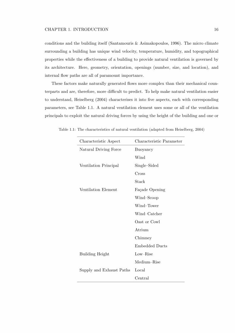
These factors make naturally generated flows more complex than their mechanical coun-
terparts and are, therefore, more difficult to predict. To help make natural ventilation easier
to understand, Heiselberg (2004) characterises it into five aspects, each with corresponding
parameters, see Table 1.1. A natural ventilation element uses some or all of the ventilation
principals to exploit the natural driving forces by using the height of the building and one or
Table 1.1: The characteristics of natural ventilation (adapted from Heiselberg, 2004)
Characteristic Aspect Characteristic Parameter
Natural Driving Force Buoyancy
Wind
Ventilation Principal Single–Sided
Cross
Stack
Ventilation Element Facade Opening
Wind–Scoop
Wind–Tower
Wind–Catcher
Oast or Cowl
Atrium
Chimney
Embedded Ducts
Building Height Low–Rise
Medium–Rise
Supply and Exhaust Paths Local
Central
CHAPTER 1. INTRODUCTION 17
more supply and exhaust paths.
Buildings all over the world are naturally ventilated by relying on the porosity of the
envelope and windows or other openings. Here, two types of flow path through the envelope
are identified: those that are purpose provided and those that are unintentional or adven-
titious. Use of arbitrary openings can result in uncontrolled ventilation that has negative
side effects such as occupant discomfort and high energy losses. However, it is possible to
exercise control over the flow rates through a building by ensuring high levels of air tightness.
In modern buildings these are normally below 0.5 air changes per hour (ACH) (Santamouris
& Asimakopoulos, 1996). Therefore, when considering natural ventilation in this thesis, it
is assumed that adventitious openings are kept to a minimum, and flow paths through the
building envelope are intentional and predefined.
If the architecture and micro climate of a building are favourable, natural ventilation
strategies can be employed cheaply with lower capital and running costs than mechanical
systems. Such systems need no plant room and require minimal maintenance. High flow
rates for cooling and purging are possible if enough openings are provided and there is no
fan or system noise. During periods of exceptionally warm weather, discomfort is normally
tolerated by occupants who adapt to the conditions by opening windows (or other purpose
provided openings) and changing clothing (Humphreys & Nicol, 1998).
Even in temperate climates buildings are often found to be too hot (Linden, 1999). In
these circumstances, natural ventilation can provide good indoor air quality levels, appropri-
ate thermal comfort levels, and a reduction in the cooling loads of the buildings. The latter
may be achieved through the use of night or nocturnal cooling techniques. At night, the
external temperature drops below the internal temperature. This fact is exploited during the
summer months by drawing cooler air inside to increase the dissipation of heat stored in the
fabric of the building. The warmer air is then exhausted leaving the air and fabric tempera-
tures lower than they might otherwise have been. Natural ventilation also helps occupants to
relate to external conditions over their internal environment and exercise control, which can
increase tolerance to a range of thermal conditions (Nicol & Humphreys, 2002; Hummelgaard
et al., 2007). Occupant performance and attendance may also be improved by a naturally
ventilated indoor environment (Mendell & Heath, 2005; Shendell et al., 2004).
Natural ventilation is not suited to every type of building or every environment, and so its
CHAPTER 1. INTRODUCTION 18
drawbacks are now discussed. Buildings with a deep plan or many individual rooms face air
distribution problems that are difficult to solve without mechanical assistance. Furthermore,
those that suffer from large heat gains may find that the lower mean flow rates provided by a
natural ventilation strategy are not sufficient to dissipate them, and so mechanical ventilation
may be more suitable. If a building is located in a noisy and polluted area, their ingress may
be a health risk to occupants (Stansfeld & Matheson, 2003; Laxen & Noordally, 1987). Some
designs may unwittingly incorporate security risks, such as large openings situated at ground
level.
Even if a building is perfectly designed for natural ventilation and in a relatively open
location, its biggest drawback is that it is subject to the whims of the weather. UK wind
speeds fluctuate throughout the year, changing with the seasons. They may be estimated for a
particular region with the help of annual average tables produced by the Meteorological (Met)
Office and the Chartered Institute for Building Services Engineers (CIBSE). For example,
these tables suggest that at Heathrow Airport near London, wind speeds and are greater
than 2 m/s for 70% of the year (CIBSE, 2006a, Table 2.42). CIBSE (2005a) suggests that
“the wind speed coincident with the temperature that is not exceeded for 99.6% of the
time is in excess of 3.5 m/s for all UK locations.” In some parts of the UK wind speeds
are much higher, particularly in the winter, and so natural ventilation may not be suitable
where the ingress of cold air causes discomfort, condensation, or high energy loss. At other
times, particularly in mid summer, hot windless days are experienced. Here it can be argued
that these days are infrequent and discomfort may be felt whatever the ventilation strategy.
Furthermore, some public buildings, such as schools, are unoccupied when these conditions
are most likely to occur. Nevertheless, the point is that the fluctuation of wind speeds makes
the control of flow rates difficult to manage and can lead either to high energy losses or air
quality problems.
Despite the drawbacks, a natural ventilation strategy remains a viable method of ventilat-
ing a building, satisfying the needs of its occupants without excessive energy consumption or
harmful bi–products. Therefore, it can be said that natural ventilation is a sustainable tech-
nology, meeting the three pillars of sustainable development: the social, the environmental,
and the economic (Porritt, 2005). It is important and warrants study. Why? It has already
been said that natural ventilation flow paths are complex, and so if such strategies are to be
CHAPTER 1. INTRODUCTION 19
designed well, the physics must be understood. To do this the effects of each of the driving
forces, the micro climate, the characteristics of air flow in and around the building, and the
effect of varying the opening type, size, and location, must all be determined. There are a
variety of strategies that have individual advantages and challenges, but a designer must be
able to specify a natural ventilation scheme that meets the guidelines of the time.
Heiselberg’s classification (see Table 1.1, p. 16) shows that natural ventilation is achieved
using three main principals. The single–sided principal uses one or more openings on a single
facade and relies on wind or buoyancy to drive air flow. The net value of these forces is
often small and so flow rates are low. Consequently, the penetration of the flow is restricted.
Cross ventilation uses air entering through a facade on one side of a building and exiting on
the other. The flow rates are more reliable than single–sided ventilation and it is easier to
achieve good penetration, subject to a clear flow path free from internal obstacles. This can
also be a constraint, as the internal space relies on an open–plan interior for the best results.
Finally, stack ventilation uses flow generated by the difference between internal and external
temperatures and is so called because of the analogy with flows through a chimney stack
(Etheridge & Sandberg, 1996). The pressure difference between the two zones is augmented
by a long duct that terminates at roof level. Air enters the building through low level openings
and is drawn through the room before entering the duct. Greater flow rates are achieved in
the winter, while the flow direction can reverse in summer when the external temperature is
greater than the internal temperature. A back–draught can occur when the stack pressure
cannot overcome the static pressure of the cold air above it.
These ventilation principles may be achieved using one or more ventilation elements. The
most important types are listed in Table 1.1 and each has its own specific technical and
architectural possibilities and consequences (Heiselberg, 2004). A wide variety of natural
ventilation elements can be seen in vernacular architecture all over the world. A wind–tower
is a chimney that rises above roof level so that it is incident to the wind whatever its direction.
An area of negative pressure forms at the top of the chimney providing suction. This device
and can be seen in the Pantheon in Rome, built by Agrippa in 27 AD (McCarthy, 1999). A
derivative is the oast–house, used to dry hops in the Kent countryside. However, in order to
provide protection from the weather, its opening is turned away from the wind. To be most
effective it must be omni–directional and rotate according to the direction of the wind, thus
CHAPTER 1. INTRODUCTION 20
adding cost and maintenance implications. Wind–scoops turn their opening directly into
the wind and are traditionally common in areas where the wind blows from a predominant
direction. In the Sind district of Western Pakistan, wind–scoops have been a prominent
feature of the skyline for the past 500 years, where despite the multi–storey architecture of
the buildings, air is channeled into every recess of the interior (Rudofsky, 1977a,b). The
history of the wind–scoop is now known to date back to at least 1500 BC because drawings
of houses with roof mounted wind–scoops, known colloquially as a Malqaf, have been found
in Egyptian tombs (Roaf, 1982).
An amalgamation of these principals is found in the wind–catcher, which consists of a
tower subdivided to contain several shafts, each connected to a vertical face. The wind–
catcher is known in Iran as a Badgir where their use has been reliably traced to the 14th
century, although a hypothesis of pre–Christian construction is, to date, uncorroborated
(Roaf, 1982). In Iran, the brick structure of the wind–catcher heats up during the day and
so it acts like a chimney, expelling hot air from the building (Roaf, 1982). When the wind
blows, a positive pressure difference is created across the windward shafts, channelling air
into a building. Conversely, a negative pressure difference across the leeward shafts draws
stale air out of the building. A draw–back of this element is that the wind and buoyancy
forces can act against each other reducing its efficiency.
Natural ventilation principles and vernacular elements can be seen incorporated into mod-
ern architecture. The Queens Building at De Montfort University, the Coventry University
Library (Simons & Maloney, 2003), Portcullis House in the City of Westminster, and Swiss Re
(also known as The Gherkin) in the City of London are four high profile examples. There are
an increasing number of recently devised natural ventilation elements available to a designer
today, such as the Wing Jetter, in addition to modern–day versions of traditional elements
such as the wind–catcher (see Khan et al., 2008).
When used in areas where the wind is consistent and strong, modern wind–catchers have
several key advantages that make them attractive to building services engineers. Firstly, a
wind–catcher can function autonomously or with additional low level envelope openings. By
locating them on the top of a building, the pollution content of the supplied air is lower than
at street level (Laxen & Noordally, 1987). They can also be used to supply air into a building
with a deep plan and multiple storeys. When compared to other modern elements (see Khan
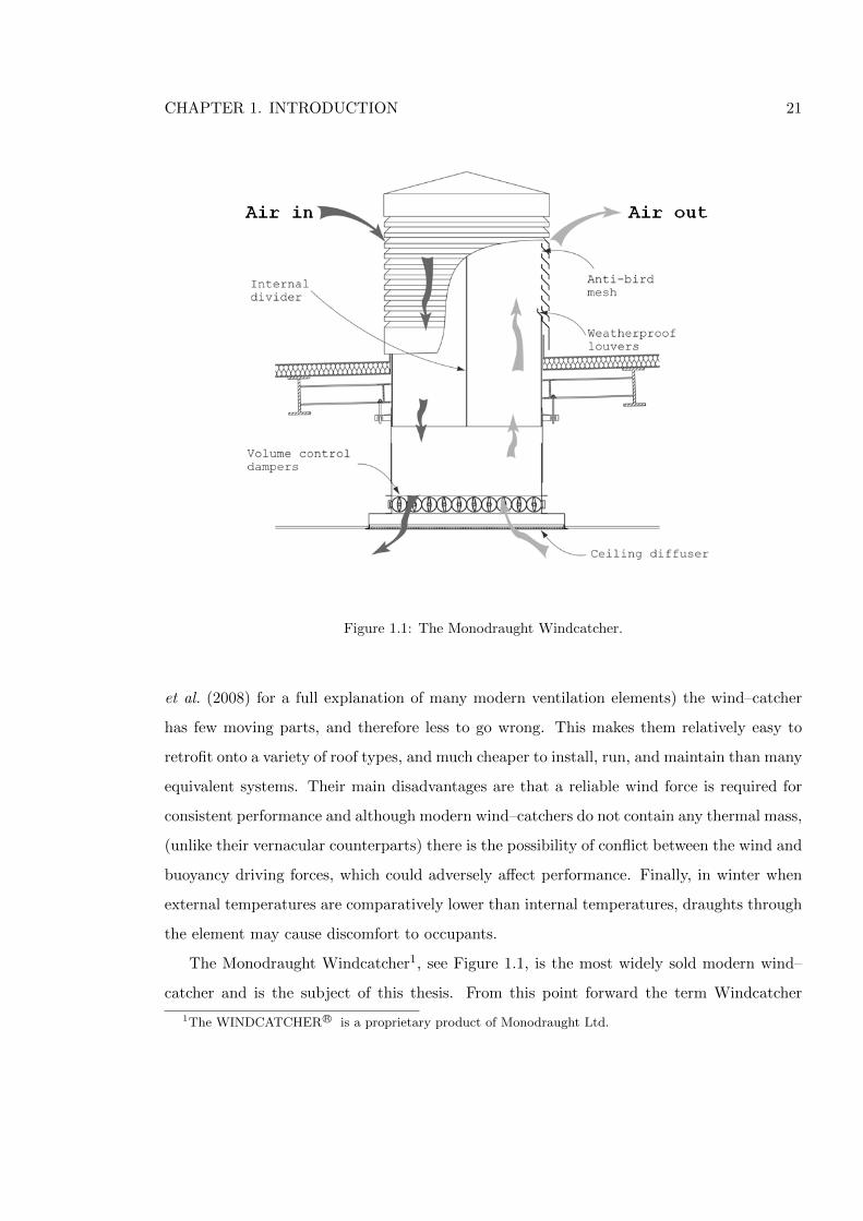
CHAPTER 1. INTRODUCTION 21
Figure 1.1: The Monodraught Windcatcher.
et al. (2008) for a full explanation of many modern ventilation elements) the wind–catcher
has few moving parts, and therefore less to go wrong. This makes them relatively easy to
retrofit onto a variety of roof types, and much cheaper to install, run, and maintain than many
equivalent systems. Their main disadvantages are that a reliable wind force is required for
consistent performance and although modern wind–catchers do not contain any thermal mass,
(unlike their vernacular counterparts) there is the possibility of conflict between the wind and
buoyancy driving forces, which could adversely affect performance. Finally, in winter when
external temperatures are comparatively lower than internal temperatures, draughts through
the element may cause discomfort to occupants.
The Monodraught Windcatcher1, see Figure 1.1, is the most widely sold modern wind–
catcher and is the subject of this thesis. From this point forward the term Windcatcher
1The WINDCATCHERR© is a proprietary product of Monodraught Ltd.
CHAPTER 1. INTRODUCTION 22
refers to the Monodraught product whereas the term wind–catcher will refer to the vernac-
ular generic element. The Windcatcher is made from glass reinforced plastic, and contains
weatherproof louvres and an anti–bird mesh. Ducts channel air to and from the room where
at its base a series of flow control dampers are protected by a grill. At the present time,
only limited scientific performance data exists, and it is not possible to fully quantify their
performance, particularly in–situ.
Over 5500 Windcatcher elements have been delivered since 2002, with 5% to hospitals,
12% to offices, and 70% to UK schools (Monodraught, 2009). To date, Windcatchers have
been fitted to over 1100 UK schools, thus making school buildings a special case, and the
reasons for choosing a Windcatcher to ventilate a school worthy of further investigation.
1.4 School Buildings
Children are particularly susceptible to poor IAQ (Mendell & Heath, 2005) yet the quality
of indoor air and ventilation rates in many UK schools are often shown to be inadequate
(Mumovic et al., 2009). Similarly, children are also negatively affected by noise (Shield &
Dockrell, 2003) which is often found to be above acceptable levels in UK schools (Shield &
Dockrell, 2004). The UK Government has attempted to address this problem by issuing a
series of guidelines that are specific to school buildings. Of particular relevance to Wind-
catchers are Building Bulletins (BB) 101 and 93 (DfES, 2006, 2003) that cover ventilation
and air quality, and noise, respectively. These documents set strict guidelines for levels of
carbon dioxide, relative humidity (RH), temperature, and noise for all types of school and
classroom.
In 2006, the UK Government started a new wave of school construction and refurbish-
ment with a budget of 45 billion that is expected to continue until 2020 (Mumovic et al.,
2009). Traditionally, schools have always had a narrow plan architecture and been natu-
rally ventilated, but today schools are more air tight, use deeper plans, maximise use of
floor space, and have an increased quantity of information and communication technology
(ICT) equipment (DfES, 2006). Until recently, mechanical ventilation systems were being
considered to dissipate increasing heat gains and provide sufficient ventilation for a positive
learning environment. However, schools are found to consume 10% of all energy used in
CHAPTER 1. INTRODUCTION 23
the commercial and public buildings sector and expenditure on building infrastructure is 7%
of the total education budget per student, which is more than the relative operating costs
of an office building (see Pegg, 2008). Buildings that are naturally ventilated cost between
10—15% less than those that are mechanically ventilated (DfES, 2006) and so natural venti-
lation strategies are actively encouraged in school design. Section 4 of BB101 advocates the
use of purpose–designed natural ventilation strategies, as opposed to mechanical or window–
opening strategies, because they have (amongst other things) cheaper capital, running, and
maintenance costs, and greater sound insulation that reduces traffic noise. This argument
is also made by guidance on Schools for the Future (BB95) (DfES, 2002), which states that
designers should “aim for natural ventilation where possible.” ClassVent (DfES, 2005) is a
simple spreadsheet based design tool available to download from several stakeholder websites,
such as www.TeacherNet.gov.org, and can be used to choose a ventilation strategy and size a
ventilation opening. Included among its ventilation elements is a roof terminal that is similar
to a Windcatcher. In many schools Windcatchers are used to meet ventilation, IAQ, and
noise guidelines because they allow for wide plan architecture, are a low–energy technology,
and have the advantage that they can be retrofitted to a classroom.
Therefore, when considering a building type that would make an ideal case–study to
evaluate the performance of a Windcatcher, schools are an excellent choice because they
have a number of desirable properties. All schools are designed to perform the same task,
the education of children, and so they have similar occupancy densities and patterns, long
vacation periods allowing for more detailed analysis using specialist techniques, and clearly
defined IAQ benchmarks against which performance may be measured. It is for these reasons
that school classrooms are the focus of this thesis.
Finally, the evolution of a new type of school means that some of the already limited
ventilation, IAQ, and noise data collected from the UK school stock are out of date. Although
some research into new–build schools has already begun (Pegg, 2008), there is a clear need
to monitor them and the purpose–provided ventilation strategies that they employ in order
to check that they function as they have been designed to, and their performance conforms
to government standards, before establishing design and implementation best practice where
possible.
CHAPTER 1. INTRODUCTION 24
1.5 Research Aim and Objectives
The aim of this thesis is to quantify the performance of Monodraught Windcatchers used
to ventilate UK school classrooms by comparing their performance against UK government
guidelines for schools.
If a prima facie of this thesis is an acceptance that a Windcatcher can deliver air into a
building—the longevity, heavy weight construction, and beautification of vernacular wind–
catchers suggest that this is so—this project aspires to meet the following objectives in order
to quantify the performance of a Windcatcher.
The first objective is to quantify and understand the performance of a Windcatcher. An
understanding of the physics of a Windcatcher system—defined as the Windcatcher element,
ducting, dampers, and grill—will help to develop an understanding of the complex interaction
between the two driving forces, flow types through the ducts, and the energy losses through
the whole system. Additional factors that may affect performance, such as the position of the
Windcatcher element relative to architectural, topographical, and meteorological conditions
will also be considered using the limited amount of theoretical and empirical Windcatcher
data that is already published.
The second objective is to develop a detailed model that can accurately predict flow rates
through a Windcatcher system. A key performance indicator of a Windcatcher is the rate at
which it delivers air into a room and stale air is extracted, and so it is important to be able to
predict ventilation rates before choosing an appropriate size of Windcatcher for a particular
building. The semi–empirical model is similar to the envelope flow model described by others
and explicitly uses experimental data published in the literature for square Windcatchers in
order to provide a fast but accurate estimate of Windcatcher performance. Included in the
model are buoyancy effects, the effect of changes in wind speed and direction, as well as the
treatment of sealed and unsealed rooms. Although this type of model relatively common it
has never been applied to predict Windcatcher performance before.
The literature review (Chapter 2) will show that there is limited data for a Windcatcher
functioning in–situ. The third objective will address this lack through a series of case–
studies that measure key Windcatcher performance indicators such as ventilation rate, CO2
concentration, temperature, and RH. Over 70% of Windcatcher elements are installed in
CHAPTER 1. INTRODUCTION 25
more than 1100 UK schools, and so all of the case studies are of UK school classrooms.
The measurements made in each classroom are compared against the relevant government
guidelines for a school classroom.
The fourth and final objective is to compare the ventilation performance of Windcatchers
measured in–situ against those estimated by the model. The information gathered here
will feedback into the predictive model (objective 2) and augment the understanding of
Windcatcher functionality and performance (objective 1).
1.6 Thesis Outline
It is intended that this thesis will make a detailed contribution to the understanding of
Windcatcher performance. The techniques for predicting flow through Windcatcher systems
will be useful as design tools and the case studies will serve as valuable examples of the
performance of Windcatchers in practice. The collection of chapters that make up this
thesis will guide the reader through the journey of research that leads to the conclusions in
Chapter 8.
Chapter 2 provides a detailed review of the drivers for research and other peer–reviewed
literature that has influenced this work. The review considers IEQ parameters with a focus
on schools and the effects of poor air quality on their occupants. Consideration is given to the
constituents of good IAQ and the methods for achieving it. Natural ventilation methods are
acknowledged as a method for providing good IAQ in school classrooms and the Windcatcher
is considered as a natural ventilation element that could be used to meet current government
requirements.
Chapter 3 considers the need for a designer to quickly, accurately, and easily predict flow
rates through a Windcatcher system in order to correctly size the system for a particular
application. Estimating the performance of the Windcatcher is complicated by complex flow
patterns and the interaction between the two driving forces. Therefore, in order to realise a
more accurate understanding of the energy losses inside a Windcatcher it is necessary to study
the air flow in detail. This is done by developing an analytic model for a variety of situations,
based upon conservation of energy and mass. By explicitly using existing experimental data
to quantify the energy losses, a semi–empirical model is formulated whose predictions are
CHAPTER 1. INTRODUCTION 26
compared against experimental data given in the literature.
Chapter 4 introduces each of the case–study school buildings that have been chosen to
show how Windcatchers perform in–situ and in a variety of environments. Because over 70%
of Windcatcher systems are installed into school buildings, all of the case study buildings are
schools. Therefore, the case–studies also have a secondary function as data collected from
them will contribute to the limited number of published reviews of air quality and ventilation
rates in UK school buildings. The parameters of each building are also compared against
similar case studies in the literature.
Chapter 5 presents the data recorded in each case–study buildings so that it can easily be
compared to government benchmarks and the performance of the Windcatcher systems can
quickly be identified. The Chapter will also detail the methodologies employed to measure
the IAQ, ventilation, and noise, highlighting merits and faults, and determining the reliability
of each of the data sets, which are then compared against similar sets in the literature.
Chapter 6 seeks to corroborate the semi–empirical model by comparing its estimations of
flow rates through a Windcatcher system with those measured in the case study buildings
and in literature.
Chapter 7 draws together the themes from the previous chapters to discuss general recom-
mendations for the use and application of Windcatchers, the ability of Windcatcher systems
to meet current guidelines, and the transferability of these observations to other building
types.
Chapter 8 makes conclusions based upon the observations of the preceding chapters.
Chapter 9 discusses further work that could be carried out to enhance the current knowl-
edge of the Windcatcher system.
Finally, the proceeding chapters contain a list of all references and appendices.
CHAPTER 2. LITERATURE REVIEW 27
Chapter 2
Literature Review
2.1 Indoor Environment Quality and Ventilation
Most people spend 80–90% of their lives inside some type of building, yet there is a strong
belief that the indoor environment may pose more of a risk to human health than the outside
(Bako-Biro, 2004). But what exactly is health? The World Health Organisation (WHO) has
a longstanding and wide definition:
Health is a state of complete physical, mental, and social well–being and not merely
the absence of disease or infirmity. (WHO, 1946)
Providing good health to each occupant of a building is not straightforward if each of
these five human factors must be considered. There are many stimuli such as the thermal
conditions, air quality, noise, and light that effect each occupant differently. The effects may
be direct, impairing concentration for example, or indirect, affecting productivity (Mendell
& Heath, 2005). If these stimuli are not addressed they can be the cause of ill–health that
manifests itself in one of two forms. The first is through a set of symptoms that have a clear
etiology, and are known as a Building Related Illness (BRI) (Bako-Biro, 2004). Bako-Biro
classifies them into three groups:
1. Airborne infectious diseases (Legionnaires’ disease, Pontiac fever, airway infections);
2. Hypersensitivity diseases (allergic asthma, rhinitis, and pneumonitis);
CHAPTER 2. LITERATURE REVIEW 28
3. Toxic reactions (carbon monoxide, pesticides).
When there is a clear link between cause and effect, it is relatively simple to address the
source of the BRI. However, associations are not always clear and although symptoms may
be recognisable, the causes are less certain. Therefore, a second group is identified where the
symptoms are known as Sick Building Syndrome (SBS), described by Apte et al. as:
A set of adverse health or discomfort symptoms that individuals experience when
they spend time indoors, particularly in office buildings, and that lessen while away
from the building. (Apte et al., 2000)
Apte et al. go on to classify symptoms into four groups based upon the area of the body
where they occur:
1. Upper respiratory and mucosal (dry, itchy, and sore eyes, nose, sinus, or throat);
2. Lower respiratory (cough, tight chest, breathing problems);
3. Neuro–physiological (headache, mental fatigue, dizziness etc.);
4. Skin irritation (itching, stinging, dryness, or reddening).
The lack of specific causative effects does not mean that SBS cannot be cured. By
addressing key indoor environment quality (IEQ) factors, most notably by increasing the
ventilation rate, the frequency and prevalence of symptoms can be reduced (Seppanen et al.,
1999).
A relationship between ventilation and positive aspects of IEQ is established by many
studies in the literature because ventilation is a means of regulating the thermal comfort of
the occupants and atmospheric pollutants that determine the overall indoor air quality (IAQ).
The results of a survey of occupants in 26 offices across Europe show that the “approval of
levels of warmth and air quality are more important than levels of lighting or humidity”
(Humphreys, 2005). Now the reasons why good ventilation can be effective in the provision
of good IEQ are considered. The relative warmth of occupants is governed by the science
of thermal comfort while air quality is related to the ventilation rate. Because ventilation
systems either generate noise or allow noise ingress, its contribution to IEQ is also evaluated.
CHAPTER 2. LITERATURE REVIEW 29
2.1.1 Thermal Comfort and Ventilation
Early studies into the thermal comfort of the occupants of buildings are directly related to
temperature (see Nicol, 1974, for example) while more recent literature suggests a psycho-
logical approach that considers parameters of past cultural and climatic experiences, and
expectations (see Auliciems, 2001). Two distinct approaches to thermal comfort are dis-
cussed within the literature: the Heat Balance model; and the model of Conceptual Thermal
Adaptation. The first approach suggests that comfort is a “universally definable state of
affairs, the other that it is a social–cultural achievement” (Chappells & Shove, 2005). How-
ever, although each approach to the achievement of thermal comfort may differ, the definition
remains consistent.
Thermal comfort is that condition of mind which expresses satisfaction with the
thermal environment. (Fanger, 1970)
The temperature that a person neither feels too hot nor too cold is known as Thermal
Neutrality. Thermal comfort is said to be achieved in a building when the highest possible
percentage of all occupants are thermally comfortable (Fanger, 1970), and acknowledges that
it is improbable to achieve complete satisfaction .
Heat balance models (also known as static or constancy models), view the “person as
a passive recipient of thermal stimuli and are premised on the assumption that the effects
of a given thermal environment are mediated exclusively by the physics of heat and mass
exchanges between the body and the environment” (Brager & De Dear, 1998) thus seeming
to ignore Fanger’s condition of mind. They are widely used by international standards (see
ISO, 2005, for example) and professional design guidelines in the UK (see CIBSE, 2006a).
The models assume that when thermal comfort is attained, heat production is equal to
the heat lost by a person and so key variables are (Fanger, 1970):
• Activity level and metabolism (heat production by the body);
• Thermal resistance of clothing;
• Air temperature;
• Mean radiant temperature;
CHAPTER 2. LITERATURE REVIEW 30
• Relative air velocity;
• Water vapour pressure in ambient air (humidity).
The findings are based upon laboratory experiments in climate chambers that yield con-
sistent and replicable results (Brager & De Dear, 1998). The average clothing insulation
(expressed as a clo unit) and the metabolic rate (expressed as a met unit) of each occupant
are applied to the model to determine an optimum comfort temperature for a specific activity
in a particular indoor environment. Brager & De Dear (1998) point out that the calculated
results of comfort can be widely different to the actual comfort of occupants determined
by a survey. This is perhaps the obvious problem of using a model defined in a laboratory
to determine a subjective quantity, and then attempting to apply it to dynamic, real life,
conditions where factors such as demographics (gender, age, culture, economic status), con-
text (season, climate, buildings design, and function), environmental interactions (indoor air
quality, acoustics, and lighting), and cognition (attitude, preference, and expectation) are
unaccounted for (Brager & De Dear, 1998; Humphreys & Nicol, 1998).
The thermal adaption approach has been conceived more recently and hypothesises that
“if a change occurs such as to produce discomfort, people react in a way which tends to restore
their comfort” (Nicol & Humphreys, 2002), thus implying that occupants adapt to their
indoor environment. Brager & De Dear (1998) suggest that three conscious modifications, or
processes of adjustment, can be carried out by an occupant to reach thermal comfort:
1. Personal adjustment (clothing, posture, moving to a different location, consumption of
hot/cold food or beverages);
2. Technological or environmental adjustment (fans, blinds, heating);
3. Cultural adjustments (scheduling of activities, dress codes, siestas).
It is also suggested that the ability of each occupant to control their environment, be it
perceived or real, is of primary importance and so the efficiency of adaptation to an indoor
environment may be expressed in terms of available control versus exercised control versus
perceived control (Brager & De Dear, 1998).
CHAPTER 2. LITERATURE REVIEW 31
This is shown in practice by comfort surveys and indoor temperature data collected from
offices in Pakistan in the 1970s by Nicol et al. (1999). The Pakistani climate delivers a wide
variety of outdoor temperatures and so a range of corresponding indoor temperatures are
also experienced. Because the only control available to the surveyed occupants were desk
fans and the ability to change clothes, clear correlation between the use of these processes
and thermal comfort is seen in the results. Thermal comfort is deemed to be better in the
buildings with the greatest temperature variation (in some cases 13◦C to 36◦C), where the
occupants had to be adapting to their environment to remain comfortable. Here, Nicol &
Humphreys (2002) argue that it is the temperature expected in a particular circumstance
rather than an attitude to the available building services that is important, which has to be
the case in the Pakistan study. In the UK, Raja (Raja et al., 2001) reports that occupants
with access to controls such as windows, blinds, and curtains report fewer cases of thermal
discomfort. This correlates with other literature that shows the cooling effect of internal air
flow; for example, Aynsley (2008) shows that when the air temperature is above 23◦C the
body needs to lose heat in order to maintain a constant internal temperature. Then, the
percentage of the optimum cooling effect achieved by an air flow is approximately 72% at
1.27 m/s, 82% at 2.54 m/s , 90% at 3.81 m/s, and 100% at 7.62 m/s. After this peak the
cooling effect decreases to zero at around 10.16 m/s. However, it should be noted that the
data does not indicate other environmental conditions that could also affect the comfort of
occupants. However, De Dear & Brager (2002) say that the question engineers should be
asking is not “should we provide more controls?” but “how do we do it?”
The heat balance models are derived using climate chambers where the air is delivered
mechanically and is, by default, pre–conditioned. Brager & De Dear (1998) compare ther-
mal comfort data from buildings ventilated using HVAC systems with those ventilated by
natural principals and find a clear distinction in the responses of occupants that cannot be
accounted for by an adjustment to clothing or activity. Consequently, they hypothesise that
the most plausible explanation is that the previous experiences of occupants governs their
expectations, which is strongly affected by a sense of whether or not conditions are under
their control. Another advantage of a naturally ventilated (NV) building is that the internal
conditions are a function of external conditions. Therefore, occupants are able to relate to
their indoor environment visually, thermally by wearing seasonal clothing, and by making
CHAPTER 2. LITERATURE REVIEW 32
use of environmental adjustments such opening or closing windows.
Although the adaptive approach addresses Fanger’s condition of mind, a criticism of
the adaptive approach to thermal comfort is that its very complexity makes its application
to building design impossible (McCartney & Nicol, 2002). However, Brager and De Dear’s
hypothesis has been applied to develop simple control strategies that use a rolling mean of
external temperature (see here McCartney & Nicol, 2002; Nicol & Humphreys, 2002; CIBSE,
2006a; BSI, 2007).
In mechanically ventilated (MV) buildings the relationships between its occupants and
thermal comfort are also complex. Here, Brager & De Dear (2000) have shown that occupants
of MV buildings expect a very narrow bandwidth of temperature variability, and so in effect
by increasing the complexity of control systems and building services, the expectations of the
occupant is also increased.
When considering the future of thermal comfort, Chappells & Shove (2005) suggest that
rather than considering a more efficient way to maintain a standard temperature, which
is energy intensive, the meaning of comfort and the way of life associated with it should
be explored, and so existing diversity and the wide variety of occupant expectations can
be exploited, and the commitment to an unsustainable future avoided. Brager & De Dear
(2000) recommend a completely separate set of standards for NV buildings that consider the
adaptive approach.
National and international standards have been slow to consider the adaptive approach;
for example ISO Standard 7730 (ergonomics of the thermal environment) uses Fanger’s com-
fort equation that requires inputs of clo and met units (ISO, 2005). It took the American
Society of Heating, Refrigerating and Air–Conditioning Engineers (ASHRAE) until 1992 to
add an “Adaptive Comfort for NV buildings in Warm Climates” section to its standard for
Thermal Environmental Conditions for Human Occupancy (Standard 55) (see De Dear &
Brager, 2002). In the UK, CIBSE Guide A for Environmental Design (CIBSE, 2006a) details
the heat balance method employed by ISO 7730, but later considers further factors such as
age, gender, and the state of an occupant’s health.
This section has shown that thermal comfort is a highly subjective quantity, that may
be achieved by the consideration of personal, technological or environmental, and cultural
factors, and not just the internal temperature. The type of ventilation strategy has been
CHAPTER 2. LITERATURE REVIEW 33
identified as being an important factor in the delivery of thermal comfort, with occupants of
NV buildings showing a greater tolerance to differing thermal conditions when they are given
control over their environment. Moreover, by getting the internal thermal conditions right,
the direct benefits to occupants upholds their right to health, while the indirect benefits can
be considerable in terms of financial cost (see Fisk, 2000, for a full breakdown). Nicol &
Humphreys (2002) hopes that it may be possible in the future to produce thermal standards
for a building that do not “resort to specification of the indoor climate”.
Thermal comfort is normally assessed by survey; however, performing surveys can be
fraught with difficulty and dependent upon the prevailing conditions in a building. For ex-
ample, a survey carried out in extreme psychological and/or environmental conditions may
produce equally extreme responses from the surveyed occupants of a building (Nicol & Roaf,
2005). Fascinatingly, Thorn (2000) cites a survey which determined that SBS symptoms oc-
curred even after all measurable causative elements had been removed, with the real problem
being an impasse between the owner of the building, the employer, and the employees. Nicol
& Roaf (2005) feel that “surveys are therefore measuring a moving target”. The achieve-
ment of thermal comfort among occupants of a room ventilated by a Windcatcher does not
necessarily prove the functionality of a Windcatcher, but instead shows that a wide range of
desirable factors are agreeable to the majority of occupants of a room, which may be unrelated
to a Windcatcher. However, it is recognised that control of the internal room temperature is
highly important and is related to the rate of ventilation. Consequently, the measurement of
internal room temperature and external ambient temperature data are of vital importance
for achieving the aim and objectives of this research because ventilation is a key moderator of
the thermal environment, and therefore important for achieving thermal comfort among the
occupants of a classroom. Finally, no matter how intriguing the psychosocial relationships
between the occupants, the classrooms, and a Windcatcher may be, they are not of interest
here, for it is the functionality of the Windcatcher that is under test. For these reasons,
and because of the many confounding factors, the difficulties involved in surveying school
children, and because their findings will not help meet the aim of this research, surveys have
not been used in the context of this thesis.
CHAPTER 2. LITERATURE REVIEW 34
2.1.2 Indoor Air Quality and Ventilation
Ventilation is defined by the Commission for the European Communities (CEC) as “the
supply to and removal of air from a space to improve the air quality” (CEC, 1992). Because
of the amount of time people spend inside buildings, the content of indoor air has become
a dominant medium of exposure to an array of harmful pollutants. Even after 150 years of
study (see Sundell, 2004, for a full history) it is not possible to show which pollutants are
causative, only those that are important. Mølhave (2003) shows that all pollutants may be
split into two groups: gases and vapours, and viable and non–viable particulate matter.
The first group contains compounds such as nitrogen dioxide (NO2), carbon monoxide
(CO), bio–effluents [such as carbon dioxide (CO2)], volatile organic compounds (VOCs) that
include formaldehyde and paint, and reactive compounds such as ozone (O3). The second
group contains fine respirable particulate matter such as PM10s (defined as particles less than
10µm) that are a product of combustion, building materials such as asbestos, man–made fi-
bres, and organic matter that includes, mould, spores (pollen), and microbes (bacteria, fungi).
These pollutant are emitted from, or are contained in, the building fabric, textile surfaces
[furniture, carpets, blinds, curtains, see Seppanen et al. (1999)], consumer products [PCs,
printers, photocopiers, see Bako-Biro et al. (2004)], or in the ventilation source (ducting).
For specific target concentrations of selected pollutants see Liddament (1996, Chapter 2,
Table 2.1).
The concentration of a pollutant in the air of a room is a function of its rate of emission,
the rate at which unpolluted air is brought into the room, and any other factors that effects
its production. Pollutants are are controlled best at their source, but if this is not possible,
isolation, the use of sorbents, and ventilation are secondary solutions.
The WHO states under articles 25 and 29 of the Universal Declaration of Human Rights,
that all people have a right to breath healthy indoor air (WHO, 2000). Fanger (2006) says
that the quality of indoor air should be defined by its effect on humans, and so one method
determining IAQ is by determining the perception of the IAQ by the occupants based upon
bioeffluent odour (the perceived IAQ). However, the sensory responses to an indoor pollutant
are not always proportional to their toxicity and so perceived IAQ is not always a universal
measure of overall IAQ (Seppanen & Fisk, 2004). For example, the ventilation strategy
CHAPTER 2. LITERATURE REVIEW 35
can affect the perception of IAQ, and here natural ventilation has been shown to impact
favourably because fewer symptoms of SBS are reported (Fisk, 2000). Furthermore, occupants
of NV buildings are shown to be more tolerant of variations in carbon dioxide levels and
temperatures than in MV buildings (Hummelgaard et al., 2007). In many studies, CO2
and RH levels are continuously monitored over a period of time to determine their effect
on occupants; for example Bako–Biro used these parameters when looking at the effects of
ventilation on the learning performance of children in school classrooms (Bako-Biro et al.,
2008) and when determining the effects of emissions from personal computers on occupants
(Bako-Biro et al., 2004).
The chemical composition of outdoor air (by volume) consists of three dominant elements:
nitrogen (78%); oxygen (21%); and argon (1%). Other constituents make up only 0.04%,
and carbon dioxide (CO2) is now present at a mean ambient concentration of 0.0386% or
386 parts per million (ppm) (NOAA, 2009). Inside a building, Persily (1997) shows that the
measurement of CO2 over time is a very useful indication of IAQ and ventilation in a building
because it is produced as a bi–product of either human respiration or combustion. If internal
CO2 only occurs from human respiration, its rate of production is related to the number, size
(age, gender, mass), and physical activity of the occupants (see BSI, 1991; Roulet & Foradini,
2002). When the internal CO2 concentration rises above the ambient level, it can be used
as a tracer gas with which to study building ventilation (see Etheridge & Sandberg, 1996,
Chapter 12, for a number of well–established techniques). Persily is very clear that CO2
is not considered to be directly hazardous to people in the concentrations generally found
in buildings, and can only be used to indicate specific and limited aspects of IAQ, not the
overall level of IAQ. Emission of pollutants from building materials or textile surfaces may
be goverened by other factors—for example formaldehyde release is a function of RH (CEC,
1992)—and so their concentration is not generally related to the number of occupants in a
room or, therefore, CO2. Consequently some studies that choose to use CO2 as an indicator
of ventilation when studying the association between ventilation and health do not always
find a link as consistently as studies that measure ventilation directly (see here Daisey et al.,
2003; Persily, 1997).
Attempts are often made to use CO2 as an indicator of SBS (see Erdmann & Apte, 2004,
for example), although SBS itself does “not indicate either a particular exposure or a specific
CHAPTER 2. LITERATURE REVIEW 36
disease” (Apte et al., 2000). Furthermore, some studies have attempted to link the internal
CO2 concentration with health, performance, and attendance issues. An early example is
reported by Myhrvold et al. (1996) who show [with limited data, see Mendell & Heath
(2005)] correlations between SBS symptoms and CO2 concentrations above 1500 ppm, while
lower ventilation levels correspond to increased CO2 concentrations that they associate with
reduced work performance. High CO2 concentration has also consistently been found to be
associated with increased sick leave when used as an indicator of ventilation in offices (Milton
et al., 2000) and school classrooms (Shendell et al., 2004). When reviewing over twenty
studies that measured CO2 concentrations and SBS symptoms in non–domestic buildings,
Seppanen et al. (1999) found that the majority showed an increase in SBS symptoms with
higher CO2 concentrations, while in a similar study Apte et al. (2000) found a similar relation
ship between CO2 concentration and health. A threshold value, below which reductions in
CO2 concentrations would not be associated with further decreases in health symptoms was
not ascertained by Seppanen, but Apte suggests a maximum acceptable concentration of
1000 ppm. Furthermore, Seppanen’s analysis shows that SBS symptoms continue to decrease
even as CO2 concentrations drop below 800 ppm. Other large scale studies (see Smedje et al.,
1997, who measured IAQ in school classrooms) found “no significant relationships between
complaints about IAQ and air exchange rate or concentration of carbon dioxide”. Apte et al.
(2000) states that negative associations should not be interpreted as evidence that ventilation
plays no part in the prediction of the prevalence of SBS symptoms in buildings, because we
already know that there is evidence of a link between the two (see Seppanen et al., 1999, for
example). The reason why CO2 is often used as indicator of some occupant response to their
indoor environment such as IAQ, SBS, or performance, is because it is easy to measure over
a long period of time, whereas long term measurement of ventilation is more problematic,
intrusive, and expensive. There is no direct link between CO2 and poor IAQ or SBS health
symptoms, and so inaccuracies in the data can occur, but the literature does generally agree
that high levels of carbon dioxide (above 1000 ppm) will increase the statistical probability
of SBS symptoms (Apte et al., 2000).
The pressure of air is related to the amount of moisture contained within it; the more
water molecules present in a sample, the higher its pressure will be. Relative humidity (RH)
is a ratio of the vapour pressure of a sample of air and the saturated vapour pressure of
CHAPTER 2. LITERATURE REVIEW 37
air at the same temperature expressed as a percentage (McMullan, 2002). Like CO2, it is
difficult to be specific about the levels required for thermal comfort and good IAQ, although
levels between 30–70% are thought to be acceptable (CEC, 1992). However, unlike CO2, RH
is a direct cause of poor IAQ through the release of formaldehyde (CEC, 1992) and can be
directly related to the number of occupants because, in a sedentary environment, up to 25%
of the body’s excess heat is lost through transpiration; the evaporation of moisture through
perspiration and breathing (Liddament, 1996). Furthermore, this can rise to between 50–80%
when activity and temperature increase. The rate of human tranpiration is reduced by high
RH and so leads to discomfort, and is increased by a low RH that leads to dehydration.
By using a climate chamber to introduced pollutants (such as floor varnish) to occupants,
Fang et al. (1998) report that with a constant level of pollution, temperature and RH have
a strong and significant impact on the perception of IAQ and that perceived IAQ decreases
with increasing air temperature and RH. But, if pollution levels increase, the impact of
temperature and RH on the perception of IAQ decreases. Finally, the influence of pollution
on perceived IAQ decreases with increased air temperature and humidity. So, for higher
levels of temperature and RH, additional pollutants are less important than they are at lower
humidity.
It is also known that the propagation of dust mites increases when RH levels are in the
region of 70–80% and that RH levels correlate directly with the production of fungal spores
(Jones, 1999). This is important because at higher levels of RH, concentrations of alternaria
(a mold allergen) in the air and dust mite antigens in floor dust are increased. Note here that
both are associated with a higher prevalence of respiratory symptoms (Fisk, 2000). Mold has
also been linked with high RH in some American schools (Daisey et al., 2003). Consequently,
it is recommended during the winter that RH levels are reduced below 45% for a period of
time to reduce dust mite numbers (CEC, 1992), but this can lead to other problems because
tests in offices find that RH levels below 25% in winter cause symptoms such as the dryness of
the nose and throat (Jaakkola & Miettinen, 1995). Mechanical systems have an advantage in
these circumstances because they can modify the humidity of incoming air. When studying
workers in 41 offices in Helsinki, Jaakkola & Miettinen (1995) found that workers in MV
and air–conditioned office buildings (with and without humidification and air recirculation)
experience more work–related symptoms of SBS when compared with those in NV buildings.
CHAPTER 2. LITERATURE REVIEW 38
Steam, evaporative humidification, and air recirculation are considered as determinants of
the symptoms. In places where the winters are warm and humid, allergies to dust mites are
more common (Daisey et al., 2003), and so the importance of monitoring RH in such climates
during the winter season are obvious.
When the ventilation rate through a room is compared against direct and indirect oc-
cupant responses to IAQ there are a greater number of statistically significant relationships
than for CO2. For example, direct occupant responses are demonstrated by considering the
relationship between health symptoms, here categorised as SBS symptoms, and ventilation
rate using the responses of nearly 30,000 occupants of non–domestic buildings. Seppanen
et al. (1999) developed an indication of relative risk to show that the probability of SBS
symptoms occurring at low ventilation rates, rather than high, are 1.1–6 times more likely.
Here, high and low ventilation rates are defined as up to 20 litres per second per person (l/s –
person) and below 10 l/s – person, respectively. The results are not definitive and Seppanen
& Fisk (2004) point out that there is no threshold ventilation rate above which the relative
risk of SBS symptoms reduces to unity, and that the direct benefits to occupants decrease in
magnitude per additional unit of ventilation. However, they also show a statistical increase in
the worsening in a least one health outcome when the ventilation rate is below 10 l/s – person;
similar results are also obtained by Wargocki et al. (2000) and Apte et al. (2000). Wargocki
et al. (2002) show that the perceived IAQ of occupants, and their comfort, increases with
the per capita ventilation rate, and that outdoor supply rates should exceed 25 l/s – person
to reduce the risk of SBS symptoms and short–term sick leave, and to increase productivity.
This ventilation rate is significantly higher than those specified by all national standards for
an office space or a classroom, would be highly energy intensive, and would only deliver a
small relative benefit to the occupants (see Seppanen & Fisk, 2004).
The majority of studies are carried out in MV offices with HVAC systems, although
some exist for NV buildings. When the two types of ventilation method are considered as
confounding factors, Seppanen & Fisk (2004) reports that “relative to NV buildings there is
a statistically significant increase in the prevalence of one or more SBS symptoms in HVAC
buildings.” In fact, a lower prevalence of SBS symptoms among occupants of NV buildings
was found despite lower ventilation rates (Seppanen et al., 1999).
There are also a number of significant studies that consider the indirect responses of
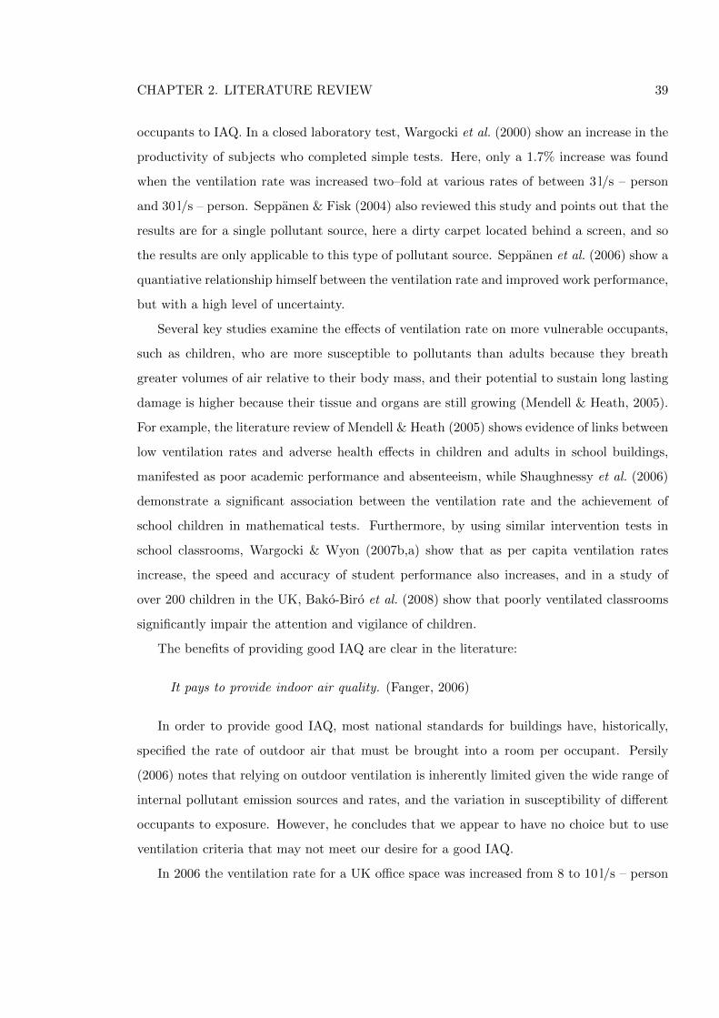
CHAPTER 2. LITERATURE REVIEW 39
occupants to IAQ. In a closed laboratory test, Wargocki et al. (2000) show an increase in the
productivity of subjects who completed simple tests. Here, only a 1.7% increase was found
when the ventilation rate was increased two–fold at various rates of between 3 l/s – person
and 30 l/s – person. Seppanen & Fisk (2004) also reviewed this study and points out that the
results are for a single pollutant source, here a dirty carpet located behind a screen, and so
the results are only applicable to this type of pollutant source. Seppanen et al. (2006) show a
quantiative relationship himself between the ventilation rate and improved work performance,
but with a high level of uncertainty.
Several key studies examine the effects of ventilation rate on more vulnerable occupants,
such as children, who are more susceptible to pollutants than adults because they breath
greater volumes of air relative to their body mass, and their potential to sustain long lasting
damage is higher because their tissue and organs are still growing (Mendell & Heath, 2005).
For example, the literature review of Mendell & Heath (2005) shows evidence of links between
low ventilation rates and adverse health effects in children and adults in school buildings,
manifested as poor academic performance and absenteeism, while Shaughnessy et al. (2006)
demonstrate a significant association between the ventilation rate and the achievement of
school children in mathematical tests. Furthermore, by using similar intervention tests in
school classrooms, Wargocki & Wyon (2007b,a) show that as per capita ventilation rates
increase, the speed and accuracy of student performance also increases, and in a study of
over 200 children in the UK, Bako-Biro et al. (2008) show that poorly ventilated classrooms
significantly impair the attention and vigilance of children.
The benefits of providing good IAQ are clear in the literature:
It pays to provide indoor air quality. (Fanger, 2006)
In order to provide good IAQ, most national standards for buildings have, historically,
specified the rate of outdoor air that must be brought into a room per occupant. Persily
(2006) notes that relying on outdoor ventilation is inherently limited given the wide range of
internal pollutant emission sources and rates, and the variation in susceptibility of different
occupants to exposure. However, he concludes that we appear to have no choice but to use
ventilation criteria that may not meet our desire for a good IAQ.
In 2006 the ventilation rate for a UK office space was increased from 8 to 10 l/s – person
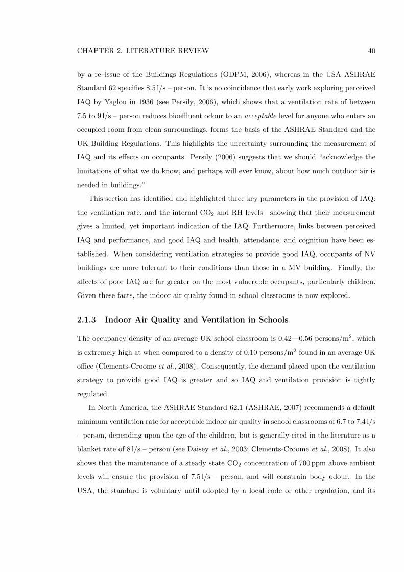
CHAPTER 2. LITERATURE REVIEW 40
by a re–issue of the Buildings Regulations (ODPM, 2006), whereas in the USA ASHRAE
Standard 62 specifies 8.5 l/s – person. It is no coincidence that early work exploring perceived
IAQ by Yaglou in 1936 (see Persily, 2006), which shows that a ventilation rate of between
7.5 to 9 l/s – person reduces bioeffluent odour to an acceptable level for anyone who enters an
occupied room from clean surroundings, forms the basis of the ASHRAE Standard and the
UK Building Regulations. This highlights the uncertainty surrounding the measurement of
IAQ and its effects on occupants. Persily (2006) suggests that we should “acknowledge the
limitations of what we do know, and perhaps will ever know, about how much outdoor air is
needed in buildings.”
This section has identified and highlighted three key parameters in the provision of IAQ:
the ventilation rate, and the internal CO2 and RH levels—showing that their measurement
gives a limited, yet important indication of the IAQ. Furthermore, links between perceived
IAQ and performance, and good IAQ and health, attendance, and cognition have been es-
tablished. When considering ventilation strategies to provide good IAQ, occupants of NV
buildings are more tolerant to their conditions than those in a MV building. Finally, the
affects of poor IAQ are far greater on the most vulnerable occupants, particularly children.
Given these facts, the indoor air quality found in school classrooms is now explored.
2.1.3 Indoor Air Quality and Ventilation in Schools
The occupancy density of an average UK school classroom is 0.42—0.56 persons/m2, which
is extremely high at when compared to a density of 0.10 persons/m2 found in an average UK
office (Clements-Croome et al., 2008). Consequently, the demand placed upon the ventilation
strategy to provide good IAQ is greater and so IAQ and ventilation provision is tightly
regulated.
In North America, the ASHRAE Standard 62.1 (ASHRAE, 2007) recommends a default
minimum ventilation rate for acceptable indoor air quality in school classrooms of 6.7 to 7.4 l/s
– person, depending upon the age of the children, but is generally cited in the literature as a
blanket rate of 8 l/s – person (see Daisey et al., 2003; Clements-Croome et al., 2008). It also
shows that the maintenance of a steady state CO2 concentration of 700 ppm above ambient
levels will ensure the provision of 7.5 l/s – person, and will constrain body odour. In the
USA, the standard is voluntary until adopted by a local code or other regulation, and its
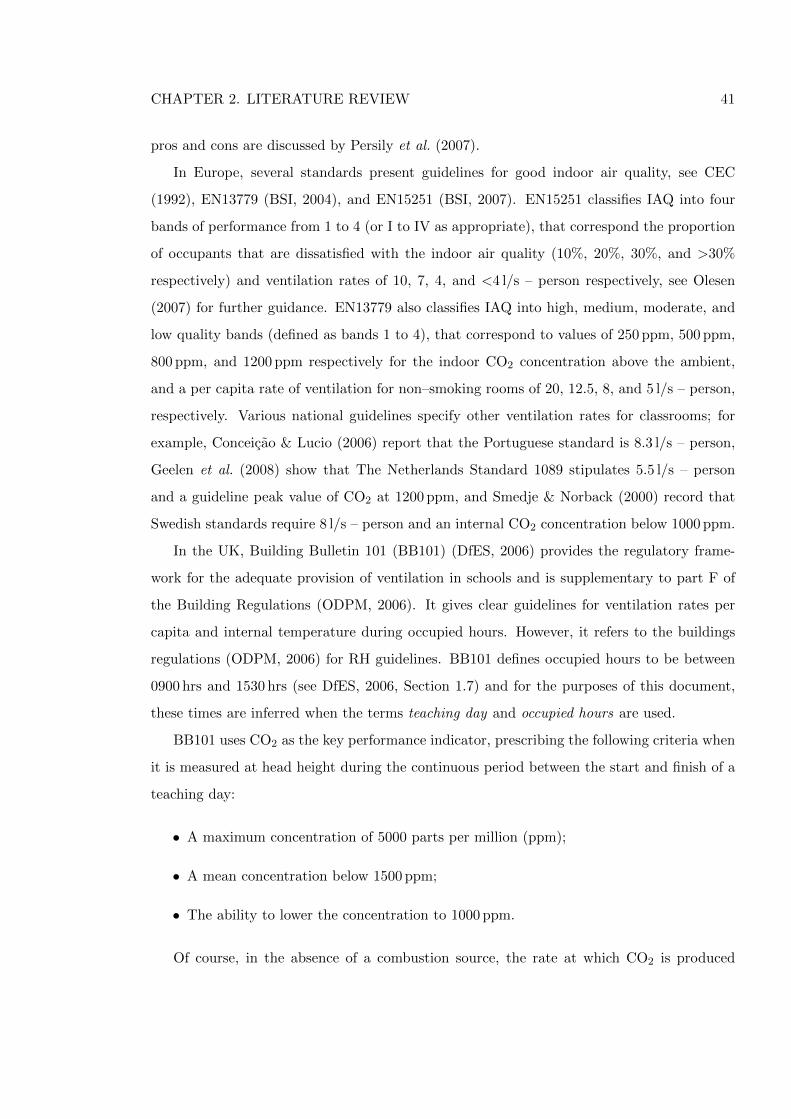
CHAPTER 2. LITERATURE REVIEW 41
pros and cons are discussed by Persily et al. (2007).
In Europe, several standards present guidelines for good indoor air quality, see CEC
(1992), EN13779 (BSI, 2004), and EN15251 (BSI, 2007). EN15251 classifies IAQ into four
bands of performance from 1 to 4 (or I to IV as appropriate), that correspond the proportion
of occupants that are dissatisfied with the indoor air quality (10%, 20%, 30%, and >30%
respectively) and ventilation rates of 10, 7, 4, and <4 l/s – person respectively, see Olesen
(2007) for further guidance. EN13779 also classifies IAQ into high, medium, moderate, and
low quality bands (defined as bands 1 to 4), that correspond to values of 250 ppm, 500 ppm,
800 ppm, and 1200 ppm respectively for the indoor CO2 concentration above the ambient,
and a per capita rate of ventilation for non–smoking rooms of 20, 12.5, 8, and 5 l/s – person,
respectively. Various national guidelines specify other ventilation rates for classrooms; for
example, Conceicao & Lucio (2006) report that the Portuguese standard is 8.3 l/s – person,
Geelen et al. (2008) show that The Netherlands Standard 1089 stipulates 5.5 l/s – person
and a guideline peak value of CO2 at 1200 ppm, and Smedje & Norback (2000) record that
Swedish standards require 8 l/s – person and an internal CO2 concentration below 1000 ppm.
In the UK, Building Bulletin 101 (BB101) (DfES, 2006) provides the regulatory frame-
work for the adequate provision of ventilation in schools and is supplementary to part F of
the Building Regulations (ODPM, 2006). It gives clear guidelines for ventilation rates per
capita and internal temperature during occupied hours. However, it refers to the buildings
regulations (ODPM, 2006) for RH guidelines. BB101 defines occupied hours to be between
0900 hrs and 1530 hrs (see DfES, 2006, Section 1.7) and for the purposes of this document,
these times are inferred when the terms teaching day and occupied hours are used.
BB101 uses CO2 as the key performance indicator, prescribing the following criteria when
it is measured at head height during the continuous period between the start and finish of a
teaching day:
• A maximum concentration of 5000 parts per million (ppm);
• A mean concentration below 1500 ppm;
• The ability to lower the concentration to 1000 ppm.
Of course, in the absence of a combustion source, the rate at which CO2 is produced
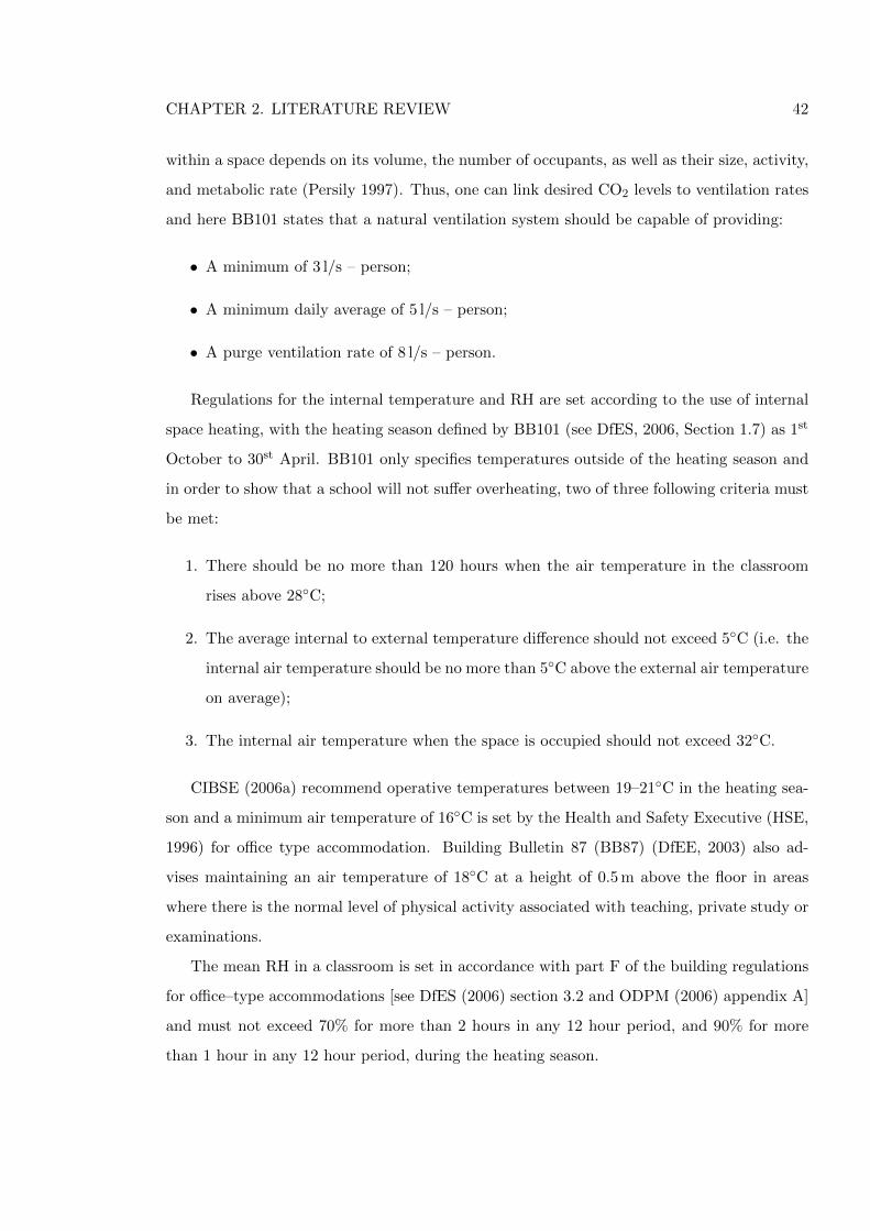
CHAPTER 2. LITERATURE REVIEW 42
within a space depends on its volume, the number of occupants, as well as their size, activity,
and metabolic rate (Persily 1997). Thus, one can link desired CO2 levels to ventilation rates
and here BB101 states that a natural ventilation system should be capable of providing:
• A minimum of 3 l/s – person;
• A minimum daily average of 5 l/s – person;
• A purge ventilation rate of 8 l/s – person.
Regulations for the internal temperature and RH are set according to the use of internal
space heating, with the heating season defined by BB101 (see DfES, 2006, Section 1.7) as 1st
October to 30st April. BB101 only specifies temperatures outside of the heating season and
in order to show that a school will not suffer overheating, two of three following criteria must
be met:
1. There should be no more than 120 hours when the air temperature in the classroom
rises above 28◦C;
2. The average internal to external temperature difference should not exceed 5◦C (i.e. the
internal air temperature should be no more than 5◦C above the external air temperature
on average);
3. The internal air temperature when the space is occupied should not exceed 32◦C.
CIBSE (2006a) recommend operative temperatures between 19–21◦C in the heating sea-
son and a minimum air temperature of 16◦C is set by the Health and Safety Executive (HSE,
1996) for office type accommodation. Building Bulletin 87 (BB87) (DfEE, 2003) also ad-
vises maintaining an air temperature of 18◦C at a height of 0.5 m above the floor in areas
where there is the normal level of physical activity associated with teaching, private study or
examinations.
The mean RH in a classroom is set in accordance with part F of the building regulations
for office–type accommodations [see DfES (2006) section 3.2 and ODPM (2006) appendix A]
and must not exceed 70% for more than 2 hours in any 12 hour period, and 90% for more
than 1 hour in any 12 hour period, during the heating season.
CHAPTER 2. LITERATURE REVIEW 43
The adverse effect of poor indoor air quality (IAQ) on the health and productivity of
building occupants is well known, see for example Mendell & Heath (2005). Poor IAQ can be
particularly detrimental to children in schools who spend approximately 12% of their time
inside school buildings, which is more than in any other building type other than their homes
(Mendell & Heath, 2005; Grimsrud et al., 2006). A range of dangerous gases such as NO2
(Stranger et al., 2008), CO (Chaloulakou & Mavroidis, 2002), and particulate matter (see
Chen et al., 2000) are known to be present in the air of school classrooms.
Most investigations of IAQ and ventilation rates in school classrooms in the literature
are for MV classrooms. Reports of internal RH and temperature are less common and are
normally considered to be of peripheral interest. For example, in North America, Godwin &
Batterman (2007) report on ventilation rates in 64 MV lower and middle school classrooms
in Michigan, USA, during the spring. The ventilation rates were found to be inadequate
in most cases with only 27% of classrooms meeting the required standard of 8 l/s – person,
and although some of the classrooms had manually opening windows, it was felt that the
weather conditions may have restricted their use, and so the results may be a function of the
season. Mean temperatures and RH are deemed to be within acceptable ranges set by the
ASHRAE handbook (see Godwin & Batterman, 2007) at 23 ± 3◦C and 38 ± 9% respectively.
This suggests that mechanical systems do not always provide adequate ventilation to meet
national standards, a finding echoed by other studies of ventilation rates in MV classrooms
in the USA and Canada. For example Grimsrud et al. (2006) report substandard ventilation
in 5 of the 8 schools they studied and very low RH of 10–20% in winter (a function of air
heating units) that is known to significantly affect comfort, and high temperatures that were
a function of poorly located or inoperable thermostats. Bartlett et al. (2004) analysed 11
portable classrooms in a single school district of British Columbia, Canada, finding that
ventilation rates and CO2 concentrations are below those required by ASHRAE Standard 62.
When making one–off spot checks of CO2 in 3801 classrooms in Washington State, Prill et al.
(2002) find that internal concentrations are over 1000 ppm in 43% of the classrooms, with
67% having a malfunctioning extract fan. Later, Shendell et al. (2004) use the same data to
show that in 50% of the classrooms, ventilation rates are less than the ASHRAE standard
rate of 7.5 l/s – person. Furthermore, they show that a rise of internal CO2 concentration
1000 ppm above external levels results in a 10–20% relative increase in student absence.
CHAPTER 2. LITERATURE REVIEW 44
Shaughnessy et al. (2006) measured a mean ventilation rate of 3.9 l/s – person in 50 US
classrooms, equivalent to half of the ASHRAE Standard 62 requirement. In addition, the
effect of reduced ventilation upon performance was measured using mathematical tests, and
showed a significant association between the two parameters.
In Hong Kong, Lee & Chang (1999, 2000) find that CO2 levels in five mechanically
and naturally ventilated Hong Kong school classrooms fail to meet the ASHRAE standard
because of overcrowding and inadequate ventilation provision. Perhaps unexpectedly, the
internal CO2 concentrations are better in the NV classrooms.
In Europe, where far fewer classrooms are MV, natural ventilation strategies using man-
ually opening windows are common. In Germany, windows are generally used to regulate the
indoor air quality and Hellwig et al. (2009a,b) report that CO2 concentrations are greater
than 1500 ppm in 7 of 15 classroom monitored in the summer and in 32 of 36 classroom mea-
sured in the winter. Classroom temperatures are also found to be too hot in the summer and
too cold in the winter, which is thought to be a function of insufficient ventilation provision
and the number of open windows. Smedje et al. (1997) reviews perceived and measured IAQ,
and the ventilation rate in classrooms from 38 schools (27% are NV) located in mid Sweden.
Ventilation rates range from 0.1 to 22.4 l/s – person with the lowest ventilation rates found in
NV classrooms. Here, the IAQ is perceived to be worse in schools with a mechanical extract
and best in schools with a mechanical supply and extract. Furthermore, at an equivalent
level of exposure to airborne pollutants, fewer complains arise from the occupants of NV
classrooms, but it is noted that the complaints are not related to the classroom ventilation
rate. Therefore, they suggest that since subjective IAQ is related to the measured exposure
levels of airborne compounds, the emission of pollutants must be higher in MV schools. In a
further study, Smedje & Norback (2000) study the links between improved ventilation with
the health and exposure of children in 39 schools in Sweden. They report that the venti-
lation rates in schools are often below the specified Swedish ventilation standard of 8 l/s –
person and above the CO2 standard of 1000 ppm. For example, they report that in 1993,
77% of investigated schools failed to meet the Swedish standard in a mixture of NV and MV
classrooms. Furthermore, the installation of new ventilation systems increased the ventila-
tion rate and reduced exposure to pollutants such as pollen, thus having a positive affect on
the frequency of asthma symptoms among the students. In Norway, Myhrvold et al. (1996)
CHAPTER 2. LITERATURE REVIEW 45
measured CO2 concentration in 35 MV classrooms finding that CO2 concentration is below
1000 ppm in 49% of classrooms, below 1500 ppm in 74% of classrooms, and above 1500 ppm
in only 26% of classrooms, indicating that 49% of classrooms would meet ASHRAE Standard
62.1 and 74% would meet the UK BB101 Standard. In the Netherlands, two sources report
the internal CO2 concentrations in a number of primary schools. Firstly, from a study of
seven primary schools in the Rotterdam, van Dijken et al. (2006) show CO2 concentrations
to be in excess of 1000 ppm for a median average of 80% of the time between April and
May, while another study of sixteen classrooms from 8 schools in Groningen shows that CO2
exceeds 1000 ppm for a median average of 77% of teaching hours in February and March.
In a study of 11 classrooms in 11 primary schools, of which three have mechanical extract
systems while the rest are NV, mean CO2 concentrations are found to be between 888 ppm
and 2112 ppm when measured between January and March, although it is not clear how the
ventilation strategy affects the internal CO2 concentration. Secondly, Geelen et al. (2008)
report that the median CO2 concentration exceeded 1000 ppm during teaching hours in 81
classes from 20 NV primary schools.
In the warmer southern European climate, Conceicao & Lucio (2006) measured the ven-
tilation rate in a Portuguese school classroom, cross ventilated using sash windows, and show
the ventilation rate to be equivalent to 2.4 l/s – person. In Greece, Santamouris et al. (2008)
measured ventilation and internal CO2 concentrations in 62 NV classrooms in Athens finding
that 29% of classrooms have a mean CO2 concentration above 1500 ppm during teaching
hours, and approximately 38%, 55%, and 77% of classroom have a mean ventilation rate
during teaching hours of less than 3, 5, and 8 l/s – person, respectively. Both of the southern
European studies show that majority of the classrooms fail to meet ASHRAE standard 62.1.
Santamouris et al. (2008) has also extensively reviewed the literature collating measure-
ments of ventilation rate and internal CO2 concentration during occupied hours from 1187
classrooms, of which 287 are NV and 900 are MV, to form a database. The database shows
that 25% and 53% of NV classrooms have a mean CO2 concentration of less than 1000 ppm
and 1500 ppm, respectively, while in MV classrooms 55% and 85% have a mean CO2 con-
centration of less that 1000 ppm and 1500 ppm, respectively. Furthermore, the database also
shows that 50%, 30%, and 5% of NV classrooms have a mean ventilation rate during teaching
hours greater than 3, 5 and 8 l/s – person, respectively, while 99%, 61%, and 50% of MV
CHAPTER 2. LITERATURE REVIEW 46
classrooms have a ventilation rate greater than 3, 5 and 8 l/s – person, respectively. All of this
data shows that school classrooms worldwide are chronically under–ventilated. Furthermore,
if geographical, architectural, and seasonal considerations are ignored, the ventilation rate in
an NV classroom is, on average, much lower than in a MV classroom, and only half of NV
classrooms would meet the UK BB101 Standard for CO2 and 30% would meet the ventilation
rate requirements.
Only a limited number of studies of ventilation and air quality in UK classrooms and their
conformity with the standards of the time have been conducted and reported in the academic
literature in recent years. Traditionally, UK schools have been designed to be NV and to
exploit natural daylight using a narrow plan architecture and manually opening windows
located in a single facade. Cross ventilation is sometimes employed using passive stacks or
clerestory (upper level) windows, but a criticism of this strategy is that the occupants often
have to choose between draughts or poor IAQ (DfES, 2006).
Although some UK school classrooms are MV, the majority employ one of the following
natural ventilation strategies:
(a) Single–sided ventilation with a single opening;
(b) Single–sided ventilation with high and low–level openings;
(c) Cross ventilation and cross ventilation with a height difference;
(d) Stack ventilation;
(e) Multiple classrooms with stack ventilation served by a corridor or atrium;
(f) Top down split duct roof–mounted ventilation (a wind–catcher).
See also Figures 2.1—2.8, beginning p. 48.
The mean ventilation rates specified by BB101 can be addressed using mechanical venti-
lation; for example, in a study of 5 MV classrooms, Mumovic et al. (2009) show that a mean
ventilation rate of 5 l/s – person is achieved in 4 of them. However, the UK Government sug-
gests that to minimise environmental impact and to reduce running and maintenance costs,
school designs should “aim for natural ventilation where possible” (DfES, 2002). This aim
is in addition to the potential of natural ventilation systems to improve IAQ and, hence, the
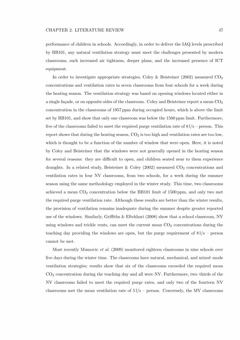
CHAPTER 2. LITERATURE REVIEW 47
performance of children in schools. Accordingly, in order to deliver the IAQ levels prescribed
by BB101, any natural ventilation strategy must meet the challenges presented by modern
classrooms, such increased air tightness, deeper plans, and the increased presence of ICT
equipment.
In order to investigate appropriate strategies, Coley & Beisteiner (2002) measured CO2
concentrations and ventilation rates in seven classrooms from four schools for a week during
the heating season. The ventilation strategy was based on opening windows located either in
a single facade, or on opposite sides of the classroom. Coley and Beisteiner report a mean CO2
concentration in the classrooms of 1957 ppm during occupied hours, which is above the limit
set by BB101, and show that only one classroom was below the 1500 ppm limit. Furthermore,
five of the classrooms failed to meet the required purge ventilation rate of 8 l/s – person. This
report shows that during the heating season, CO2 is too high and ventilation rates are too low,
which is thought to be a function of the number of window that were open. Here, it is noted
by Coley and Beisteiner that the windows were not generally opened in the heating season
for several reasons: they are difficult to open, and children seated near to them experience
draughts. In a related study, Beisteiner & Coley (2002) measured CO2 concentrations and
ventilation rates in four NV classrooms, from two schools, for a week during the summer
season using the same methodology employed in the winter study. This time, two classrooms
achieved a mean CO2 concentration below the BB101 limit of 1500 ppm, and only two met
the required purge ventilation rate. Although these results are better than the winter results,
the provision of ventilation remains inadequate during the summer despite greater reported
use of the windows. Similarly, Griffiths & Eftekhari (2008) show that a school classroom, NV
using windows and trickle vents, can meet the current mean CO2 concentrations during the
teaching day providing the windows are open, but the purge requirement of 8 l/s – person
cannot be met.
Most recently Mumovic et al. (2009) monitored eighteen classrooms in nine schools over
five days during the winter time. The classrooms have natural, mechanical, and mixed–mode
ventilation strategies; results show that six of the classrooms exceeded the required mean
CO2 concentration during the teaching day and all were NV. Furthermore, two–thirds of the
NV classrooms failed to meet the required purge rates, and only two of the fourteen NV
classrooms met the mean ventilation rate of 5 l/s – person. Conversely, the MV classrooms
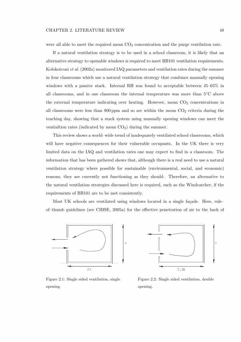
CHAPTER 2. LITERATURE REVIEW 48
were all able to meet the required mean CO2 concentration and the purge ventilation rate.
If a natural ventilation strategy is to be used in a school classroom, it is likely that an
alternative strategy to openable windows is required to meet BB101 ventilation requirements.
Kolokotroni et al. (2002a) monitored IAQ parameters and ventilation rates during the summer
in four classrooms which use a natural ventilation strategy that combines manually opening
windows with a passive stack. Internal RH was found to acceptable between 45–65% in
all classrooms, and in one classroom the internal temperature was more than 5◦C above
the external temperature indicating over heating. However, mean CO2 concentrations in
all classrooms were less than 800 ppm and so are within the mean CO2 criteria during the
teaching day, showing that a stack system using manually opening windows can meet the
ventialtion rates (indicated by mean CO2) during the summer.
This review shows a world–wide trend of inadequately ventilated school classrooms, which
will have negative consequences for their vulnerable occupants. In the UK there is very
limited data on the IAQ and ventilation rates one may expect to find in a classroom. The
information that has been gathered shows that, although there is a real need to use a natural
ventilation strategy where possible for sustainable (environmental, social, and economic)
reasons, they are currently not functioning as they should. Therefore, an alternative to
the natural ventilation strategies discussed here is required, such as the Windcatcher, if the
requirements of BB101 are to be met consistently.
Most UK schools are ventilated using windows located in a single facade. Here, rule–
of–thumb guidelines (see CIBSE, 2005a) for the effective penetration of air to the back of
Figure 2.1: Single sided ventilation, single
opening.
Figure 2.2: Single sided ventilation, double
opening.
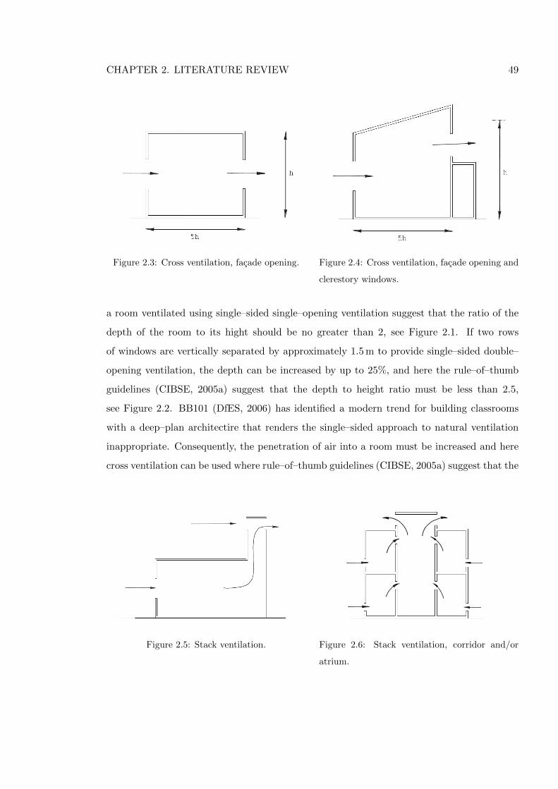
CHAPTER 2. LITERATURE REVIEW 49
Figure 2.3: Cross ventilation, facade opening. Figure 2.4: Cross ventilation, facade opening and
clerestory windows.
a room ventilated using single–sided single–opening ventilation suggest that the ratio of the
depth of the room to its hight should be no greater than 2, see Figure 2.1. If two rows
of windows are vertically separated by approximately 1.5 m to provide single–sided double–
opening ventilation, the depth can be increased by up to 25%, and here the rule–of–thumb
guidelines (CIBSE, 2005a) suggest that the depth to height ratio must be less than 2.5,
see Figure 2.2. BB101 (DfES, 2006) has identified a modern trend for building classrooms
with a deep–plan architectire that renders the single–sided approach to natural ventilation
inappropriate. Consequently, the penetration of air into a room must be increased and here
cross ventilation can be used where rule–of–thumb guidelines (CIBSE, 2005a) suggest that the
Figure 2.5: Stack ventilation. Figure 2.6: Stack ventilation, corridor and/or
atrium.
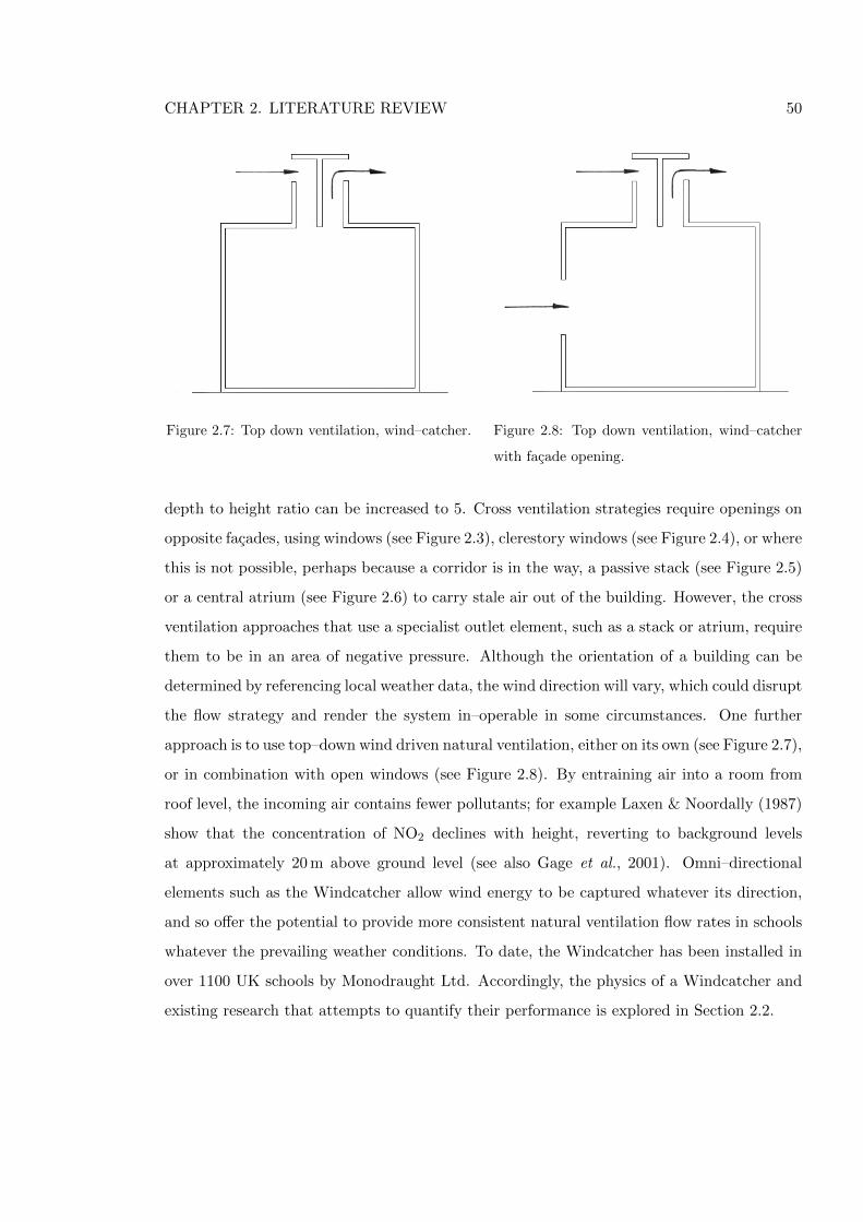
CHAPTER 2. LITERATURE REVIEW 50
Figure 2.7: Top down ventilation, wind–catcher. Figure 2.8: Top down ventilation, wind–catcher
with facade opening.
depth to height ratio can be increased to 5. Cross ventilation strategies require openings on
opposite facades, using windows (see Figure 2.3), clerestory windows (see Figure 2.4), or where
this is not possible, perhaps because a corridor is in the way, a passive stack (see Figure 2.5)
or a central atrium (see Figure 2.6) to carry stale air out of the building. However, the cross
ventilation approaches that use a specialist outlet element, such as a stack or atrium, require
them to be in an area of negative pressure. Although the orientation of a building can be
determined by referencing local weather data, the wind direction will vary, which could disrupt
the flow strategy and render the system in–operable in some circumstances. One further
approach is to use top–down wind driven natural ventilation, either on its own (see Figure 2.7),
or in combination with open windows (see Figure 2.8). By entraining air into a room from
roof level, the incoming air contains fewer pollutants; for example Laxen & Noordally (1987)
show that the concentration of NO2 declines with height, reverting to background levels
at approximately 20 m above ground level (see also Gage et al., 2001). Omni–directional
elements such as the Windcatcher allow wind energy to be captured whatever its direction,
and so offer the potential to provide more consistent natural ventilation flow rates in schools
whatever the prevailing weather conditions. To date, the Windcatcher has been installed in
over 1100 UK schools by Monodraught Ltd. Accordingly, the physics of a Windcatcher and
existing research that attempts to quantify their performance is explored in Section 2.2.
CHAPTER 2. LITERATURE REVIEW 51
2.1.4 Indoor Environmental Noise and Ventilation
The human ear is capable of responding to sound frequencies from approximately 20Hz to
20kHz, but is much more responsive to broadband noise rather than a single tone of sound
(Kinsler et al., 1982). In a building, broadband noise is the combination of direct sound from
a source and the reverberation of that sound. Ling (2001) shows that noise comes from three
sources:
1. External noise (entering a building through ventilation openings or envelope. defects)
2. Internal noise (from ventilation systems or electronic equipment).
3. Path effects (sound transported through a building via a ventilation system or building
voids).
Noise within a building is generally below 85–90 dBA and will not cause auditory damage
to the ears, however the non–auditory effects are far more dangerous to health (Stansfeld
& Matheson, 2003). Here, Stansfeld and Matheson link occupational and environmental
noise with hypertension, and aircraft and traffic noise with psychological symptoms. Aircraft
and traffic noise is associated with raised blood pressure and is also shown to impair the
reading comprehension and the long term memory of children. Furthermore, it is generally
accepted that noise has a detrimental effect upon the learning and attainment of primary
school children, who are more susceptible than adults (Shield & Dockrell, 2003).
Therefore, the investigation of noise in schools and its affect on children is of great interest.
Different types of noise (conversational babble and environmental noises for example) are
shown to produce different effects on children when performing different tasks (Dockrell &
Shield, 2006), while road traffic noise has a negative effect on the attention span of school
children (Sanz et al., 1993). More sudden noises, such as sirens, trains, or aircraft, may
affect children and teachers “disproportionately to their contribution to the overall noise
environment of a school.” (Shield & Dockrell, 2003) Other noise related quantities such as
the reverberation time and sound absorption of a classroom are a function of design and
cannot be linked directly to the ventilation system. These effects are not discussed here, but
they are discussed in a in review of literature by Shield & Dockrell (2003).
CHAPTER 2. LITERATURE REVIEW 52
The World Health Organisation (WHO, 1999) and the American Standards Institute
(ANSI, 2002) both specify background levels of noise for classrooms of 35dB LAeq during
teaching hours. In the UK, Building Bulletin 93 (BB93) (DfES, 2003) provides the regula-
tory framework for noise levels in schools. Upper limits are specified as LAeq,30min, an average
uninterrupted measurement of A weighted sound pressure level over 30 minutes in an unoc-
cupied and unfurnished classroom. Here, BB93 (DfES, 2003, Table 1.1) sets the upper limit
at 35 dBA in a conventional classroom and 40 dBA in a science and technology laboratory.
BB101 (DfES, 2006) allows an additional 5 dB LAeq,30min when the purge ventilation rate of
8 l/s – person is provided by natural ventilation. For all all other ventilation rates the BB93
limits apply.
Shield & Dockrell (2004) measured noise levels outside 142 urban schools in London, where
86% of the them were exposed to road traffic noise; the average external sound pressure level
was calculated to be 57 dB LAeq,5min. Ling (2001) reports that measurements of road traffic
noise should be measured over an 18 hour period from 0600–2400 hours, so these results
should only be considered a snapshot, but were chosen by Shield and Dockrell to be “typical
of the school day” and so avioded rush hour, arrival, departure, and play time periods.
As part of the same study, internal measurements were made inside 30 empty classrooms
where the mean background levels was found to be 47 dB LAeq,2min, which is 12 dBA above
those specified by BB93. Although the measurements were only made over periods of 2 min-
utes, continuous monitoring over a number of hours revealed that the fluctuation of noise
was minimal, and so was considered to be approximately constant. Seven of the classrooms
are reported as having audible heating/ventilation noise where mean background levels were
highest, although specific ventilation strategies are not reported. Shield and Dockrell note
that the noise levels measured in Victorian classrooms were, on average, 3.2 dBA lower than
those measured in modern classrooms and that the glazing type appeared to make no differ-
ence to classroom noise levels in this study, although it is acknowledged that the sample size
is deemed to be too small for definitive conclusions to be made. However, Shield and Dockrell
point out that background traffic noise is predominantly made up of low frequencies that are
difficult to attenuate using glazing. Most NV school classrooms must open windows to pro-
vide fresh air, thus increasing the ingress of noise (Ling, 2001). Andersen & Hopkins (2005)
show that some types of windows, here those manufactured by Velux, only need to open 2 cm
CHAPTER 2. LITERATURE REVIEW 53
(a distance determined in the laboratory and not in the field) to provide sufficient ventilation
while maintaining adequate sound insulation. However, the fact remains that background
levels in UK classrooms are already too high and opening windows increases them. A re-
cent study of noise levels in 12 UK school classrooms built since 2003 (see Mumovic et al.,
2009) shows that 50% of measured classrooms fail to meet government requirements, with all
mechanically ventilated classrooms failing to meet the internal ambient noise criteria. Most
interesting of all, the report concludes that more noise is generated internally than externally.
Noise generated by mechanical ventilation systems arises from aerodynamic turbulence
caused by fans, and contractions and expansions in its duct work that may consists of branch-
ing elements, diffusers, grills, and turning vanes (Ling, 2001). Natural ventilation systems
have comparably large openings that offer low resistance to the ingress of external noise. In
fact, the need to provide low–resistance ducts for the free–flow of air and to reduce noise
ingress is a paradox. This was found to be a problem in the Coventry University Library
where occupants applied their own acoustic lining to an exposed concrete natural ventilation
duct (Simons & Maloney, 2003).
The average broadband traffic noise found in urban areas is approximately 70 dBA (Shield
& Dockrell, 2003) and so an attenuation of 35–30 dBA must be made by the facade of the
building and any ventilation elements. One cost effective response is to line ducts with
an absorbent material. Here, a non–peer reviewed assessment of a square Monodraught
Windcatcher, of cross sectional area 0.64 m2, by the Building Research Establishment (BRE,
2005) shows that when it was tested in accordance with ISO 717–1 (ISO, 1997) and ISO
140–10 (ISO, 1991) to produce a standard acoustic difference from one room to another, the
addition of a 25 mm open cell polyurethane foam acoustic lining to a duct (of length 1.1 m)
and its partition, increases the airborne sound insulation by 11 dB. However, Oldham et al.
(2004) show that duct lining is designed to attenuate mid and high frequencies and has mixed
effects on low frequency traffic noise. A more expensive solution is to use active noise control
which Oldham et al. show can attenuate lower frequencies by around 22 dBA. De Salis et al.
(2002) offer a note of caution because badly designed active control systems can themselves
be the cause of problems. De Salis et al. suggest the use of external architectural features
such as fences or earth mounds. Dockrell & Shield (2006) advocates internal measures and
suggests using ceiling tiles, carpeting and curtains, and wall covering to absorb sound.
CHAPTER 2. LITERATURE REVIEW 54
The literature shows the negative effects of noise on the occupants of buildings, with
children affected more than adults. Most studies of noise in schools are for NV classrooms,
however there are no in–situ measurements of noise in classrooms or any other type of room
ventilated by a Windcatcher. Clearly, the need to attenuate noise through a natural venti-
lation system is at odds with the requirement to allow air to flow with as little resistance as
possible. The consideration of both factors may lead to a compromise that could negatively
affect the occupants of a room ventilated by a Windcatcher, thus making the measurement
of noise in–situ highly important.
2.2 The Measurement and Prediction of Natural Ventilation
The principals of natural ventilation have been used for millenia to ventilate human shelters
such as Bedouin tents (Roaf, 1982), houses (Rudofsky, 1977a,b; Chaichongrak et al., 2002),
and places of religious worship (McCarthy, 1999) for example. The earliest example of a spe-
cific natural ventilation element, a wind–scoop, has been found on papyrus scrolls stored in
Egyptian tombs and dated to around 1500 B.C. The fundamentals of natural ventilation the-
ory, (see Etheridge & Sandberg, 1996; Linden, 1999, for example), and a series of techniques
for making empirical measurements in the laboratory (Cook, 1998; Cook et al., 2003), and in
the field (Liddament, 1996) have been established. However, natural ventilation, which may
be defined as the flow of air between a building and its surroundings driven using naturally
occurring forces, is fraught with uncertainty. This section will show that there are still a great
many unknowns, but also that there are a number of methods that may be employed to mea-
sure and estimate natural ventilation flow rates. Those that are relevant to the investigation
of a Windcatcher are now explored.
2.2.1 Predicting Natural Ventilation Performance
Etheridge & Sandberg (1996) state that there are two basic ventilation processes (i) flow
through the skin of a building, defined as the envelope, and (ii) internal air motion.
A pressure difference across an opening in a building’s envelope creates a flow of air
through it, and the flow rate is governed by the difference between the internal and external
pressure, the geometry of the opening, and the properties of the air (Etheridge & Sandberg,
CHAPTER 2. LITERATURE REVIEW 55
1996). Air flow through a number of openings are not mutually exclusive because the total
flow must obey the principal of conservation of mass. However, these simple fundamental
principals are sometimes omitted in the literature, see Elmualim (2006a) or Li & Mak (2007)
for example.
The variability of the driving forces, and the complex flow patterns make natural venti-
lation hard to predict. Furthermore, several studies (Hunt & Linden, 2000; Li et al., 2001;
Chenvidyakarn & Woods, 2005, for example) show that air flow in a building can, under
certain circumstances, exhibit non–linear dynamics and so more than one steady–state so-
lution may exist for a single set of conditions. Consequently, the choice of methodology for
predicting natural ventilation flow rates is important and defined by the required outcome.
Methodologies used to predict the performance of natural ventilation strategies have been
categorised by Chen (2009) into the following groups:
• Analytic models.
• Empirical models
• Small–scale experimental models.
• Full–scale experimental models.
• Multi–zone models.
• Zonal models.
• Computational Fluid Dynamics (CFD) models.
Analytic models are often derived from the fundamental equations of fluid dynamics and
heat transfer, such as mass, momentum, and energy conservation (Chen, 2009), and can be
solved using methods as simple as a graph (see Etheridge, 2002, for example) or a spread sheet
(Li & Heiselberg, 2002). Analytic methods have been widely used to estimate flow behaviour
in a single zone box with high and low openings in opposite walls when the wind acts with the
buoyancy forces to form displacement ventilation, a stratified layer will form whose height can
be estimated (Linden, 1999). When the wind and buoyancy forces are in opposition, the flow
direction depends upon their relative strengths, but if flow enters from the upper opening,
CHAPTER 2. LITERATURE REVIEW 56
the internal and incoming air mix together (known as mixing ventilation) (Heiselberg et al.,
2004) and the type and patterns formed by the internal flow has consequences for the pre–
heating of incoming air in winter (Fitzgerald & Woods, 2007), or the transport of airbourne
pathogens in hospitals (Li et al., 2007) for example.
Simple envelope flow models used for the estimation of single sided ventilation through
one or more openings in a single zone, and cross ventilation through two or more openings in
a single zone when wind or buoyancy driven, have been incorporated into national standards,
see BS 5925 (BSI, 1991). Furthermore, methods for predicting the air flow through atria and
passive stacks are presented in professional literature, see (CIBSE, 2005a), and calculation
software is detailed by Liddament (1996).
One method of increasing the accuracy of analytic models is to incorporate data from
experimental measurement or advanced computer simulation to form an empirical model
that Chen (2009) describes as the “bread and butter tools for ventilation design”. These
models are used by most design handbooks, design guidelines and product catalogues for
ventilation design, see Karava et al. (2003) for example, who derive an empirical model of
flow through trickle vents.
The advantage of using a small scale model is its cost. Here, measurement or visualisa-
tion techniques are used to establish flow paths and ventilation performance once dynamic
similarity has been achieved. For example, Etheridge (2004) and Costola & Etheridge (2008)
used a wind tunnel and anemometry to measure flow through a model stack. In addition,
models placed in wind tunnels have been used to establish the characteristics of flow through
a series of simple sharp edged openings, and to derive discharge coefficients (Karava et al.,
2004). Furthermore, Sawachi et al. (2006) derived wind pressure coefficients for buildings of
different shapes and surrounding topographies, which can be applied easily to analytic mod-
els. Tables of similarly derived coefficients are also widely available, see Liddament (1996),
Orme & Leksmono (2002), and Santamouris & Asimakopoulos (1996).
In addition to the wind tunnel testing of scale models, water baths are also commonly
used to investigate the effects of buoyancy through the injection of a dyed and/or saline
solution. Because brine is more dense than water, the model is inverted and the solution
injected through the top of the model, and observations of flow paths and velocity and
density are made using shadow graphs and digital imaging techniques. For example, Gage
CHAPTER 2. LITERATURE REVIEW 57
et al. (2001) investigated the entrainment of cold air into a single zone through an inverted
chimney mounted in the ceiling model showing that “the experiments clearly demonstrate
that it is possible to use stack forces to draw ambient air down into a space from roof level
via an inverted chimney using a displacement mode of passive ventilation”, which has direct
application to the physics of a Windcatcher. Furthermore, water tank models have been
used to establish the non–linear dynamics predicted by Hunt & Linden (2000) and others,
and such experimentation is normally accompanied by a theoretical analysis and/or a CFD
study, see Heiselberg et al. (2004) for example.
Full–scale modelling can be conducted both in the laboratory and in–situ. Here, the line
between in–situ modelling and the evaluation of the ventilation performance of an existing
building blurs. Chen (2009) describes in–situ modelling as the use of an existing building to
estimate ventilation rates through a similar, hypothetical building.
In the laboratory, the performance of ventilation elements can be assessed in a wind
tunnel. Khan et al. (2008) review several full size natural ventilation elements, such as the
rotational chimney cowl, whose performance has been determined by wind tunnel analysis.
The performance of a Windcatcher has been assessed using a wind tunnel, see Elmualim et al.
(2001) and Awbi & Elmualim (2002), and these studies are discussed in Section 2.3.2.
Laboratory based climate chambers can be used to simulate a room or zone, and when
the effects of outdoor conditions are examined, a wind tunnel is used to replicate conditions.
Here, Etheridge & Sandberg (1996, Chapter 12) detail a test house used to determine the
effectiveness of the three main tracer gas techniques: the decay method, the constant injection
method, and the constant concentration method. Note that these key methods of determining
ventilation rates through a room both in the laboratory and in–situ are discussed in detail
in Section 2.2.2.
Zonal and multi–zone models are also known as Network models. Liddament (1996)
suggest considering a building as a number of zones or cells connected by flow pathways.
A multi–zone model, where each room is considered to be a zone, assumes that the air in
each room is well mixed and so is used to estimate ventilation rates, energy, and pollutant
transfer. Conversely, Chen (2009) shows that a zonal model avoids the assumption of full
mixing by dividing a single room into a finite number of cells (<1000) so that it can determine
ventilation inside a large space or deal with the effects of stratification. Chen concludes that
CHAPTER 2. LITERATURE REVIEW 58
they are difficult to develop and could be superseded by CFD models.
The use of computational fluid dynamics (CFD) models is increasing; in an overview of the
tools used to predict ventilation performance in buildings, Chen (2009) finds that over 70% of
the literature in his review used CFD. Etheridge & Sandberg (1996) state that CFD provides
a numerical solution to the partial differential equations that govern a flow field. Furthermore,
to model ventilation in a confined space where density differences caused by heating occur,
turbulence and buoyancy must also be accounted for. When the boundary conditions are
fixed and the flow is steady, the results are time averaged, but when the boundary conditions
change with time and the flow is unsteady, the calcuations are ensemble averages (Etheridge
& Sandberg, 1996). In theory, CFD brings the real world to one’s desk, yet, as with any
model, a series of assumptions have to be made about that modelled environment which
means that one can only expect qualitative information to be obtained. Consequently CFD
is often used to validate an analytic model (see Heiselberg et al., 2004; Evola & Popov,
2006), data obtained from full scale wind tunnel testing (Elmualim, 2006a; Etheridge, 2009),
or flow rates measured in an actual building (Horan & Finn, 2005), although there are a
significant number of studies that do not compare the predictions made by a CFD model
against empirically or theoretically determined flow rates, see Hughes & Ghani (2008, 2009)
for example.
2.2.2 Measuring Natural Ventilation Performance
The energy consumption and IAQ of a building are closely related to the air flow through its
envelope, thus the in–situ measurement of total air flow rates through a single zone or series
of zones will give a good indication of these parameters. The most accurate and commonly
used techniques involve the injection of a tracer gas into the atmosphere of a room and the
subsequent measurement of its concentration over time. The rate at which air free from the
tracer gas is brought into the room is determined from the concentration history. Etheridge
& Sandberg (1996) and Liddament (1996) detail three techniques. (i) The Decay Method
injects of a small amount of tracer gas into a single zone that is thoroughly mixed to establish
a uniform concentration and its exponential decay is monitored over a period of time. (ii) The
Constant Concentration method modifies the continuous rate of injection of a tracer gas into
a single zone so that a near constant concentration of a tracer gas in maintained. The volume
CHAPTER 2. LITERATURE REVIEW 59
flow rate of the tracer gas is proportional to the overall ventilation rate through the zone.
(iii) Finally, the Constant Emissions or Injection method releases a tracer gas at a steady
injection rate and mixes it into the local atmosphere so that an equilibrium concentration is
reached. This concentration is also proportional to the overall ventilation rate through the
zone.
An ideal tracer gas is one that is uncommonly found in the atmosphere; here, Niemela
et al. (1991) review three different tracer compounds determining that the completeness of
mixing through the room is the key to their performance and not their relative properties.
Most studies use sulphur hexafluoride (SF6) as a tracer gas, and determine the ventilation
rates by plotting the natural log of the concentration against time and obtaining the gradient
of the resulting straight line of negative slope by linear data regression, see Kolokotroni
et al. (2002b); Kirk (2004a); Kirk & Kolokotroni (2004b) for example. Then, the coefficient
of determination (R2) can be used as an indication of the extent of exponential decay and
thus the accuracy of mixing. Others have used CO2 because it is cheaper and more readily
available as a bi–product of respiration, see Bartlett et al. (2004); Coley & Beisteiner (2002).
Furthermore, if the number of occupants and the rate at which they emit CO2 are known,
the total ventilation rate can be estimated using the constant emission method (Roulet &
Foradini, 2002). However, because CO2 is readily found in the atmosphere, the accuracy of
this method can be low unless great care is taken to eliminate compounded equipment errors,
see Persily (1996, 1997). It is generally uncommon for errors made in the measurement of
ventilation rates using the tracer gas techniques to be discussed in the literature—an exception
is Bartlett et al. (2004)—however, Sherman (1990) estimates that overall errors are ±10%
and Persily (2006) states that they are no better than ±20%.
Cook (1998) details two further methods: the empirical tightness method (ETM) and
simplified theoretical method (STM). The ETM calculates the average air tightness by es-
timating infiltration rates when the building is pressurised to 50 Pa, which is undertaken as
standard on all new buildings. The overall ventilation rate through the building is determined
as a function of the surrounding topography and meteorological conditions, giving an estima-
tion that is approximate at best. Similarly, the STM uses a single equation that incorporates
an estimation of the effective leakage area, and factors that affect the air flow into and out
of a zone, to estimate the total air flow rate through a building. The effective leakage area
CHAPTER 2. LITERATURE REVIEW 60
is a measure of the air tightness at a reference pressure difference of 4 Pa, but can also be
extrapolated from a similar measurement made at 50 Pa. Neither of these methods are in
common use and have been superseded by the tracer gas techniques.
So, by using the tracer gas techniques, it is possible to determine the overall ventilation
rate through a room. However, it must be remembered that this is a measurement of the total
ventilation rate through a single zone and not the specific flow rate through an element such
as a Windcatcher. Because of the likelihood of a turbulent flow regime, and the non–circular
cross section of their ducts—they are triangular—this type of measurement requires highly
sensitive equipment such as an omni–directional hot–wire anemometer (see Liddament, 1996,
for details of duel wire and ultrasonic anemometers) and a series of measurements across a
section of the duct using a grid pattern to determine the average flow rate, see Douglas et al.
(1995, Chapter 6).
2.3 Measurement and Prediction of Air Flow Through a
Windcatcher
The term wind–catcher often incorporates any element that naturally ventilates a room from
roof level. However, not all devices are omni–directional, nor can they supply and extract
air simultaneously, see Montazeri & Azizian (2008) for example, and so it is argued here
that these should retain the terms wind–scoop, oast or cowl, wind–tower, chimney, or their
vernacular equivalents as appropriate. Therefore, a wind–catcher is defined as a device that
can simultaneously supply fresh air to, and extract stale air from a room at roof level whatever
the wind’s direction, and without mechanical assistance.
There are several examples reported in the literature of the measurement and prediction
of flow rates through a modern commercially produced Windcatcher, although these are not
as prevalent as those for other elements such as windows or passive stacks. Measurements
of the Windcatcher have generally been restricted to the laboratory where several method-
ologies have been employed to determine flow rates through the Windcatcher with changing
conditions. Very few studies have examined Windcatcher performance in–situ, but one study
carefully details the performance of vernacular wind–catchers.
CHAPTER 2. LITERATURE REVIEW 61
2.3.1 Quantifying the Performance of Vernacular Wind–Catchers
The wind–catcher originates from the hot arid climate of the middle–east. Over 100 examples
may still be found in the city of Yazd on the Iranian Plateau, where the prevailing winds
blow reliably at around 9 m/s. Here, Roaf (1982) has made an extensive study of the Yazdi
wind–catchers, detailing construction methods, dimensions, components, and everyday use.
The wind–catchers are a status symbol and so they are built of brick, stone, and plaster, with
most having have a rectangular cross section, although other planforms such as hexagonal are
used. They protrude, on average, 5 m above the buildings they are mounted upon, and can
be as tall as 22 m to take advantage of the higher wind speeds found at increased elevation,
see Liddament (1996). Their cross sectional areas (CSA) vary from as little as 0.32 m2 to a
huge 77 m2, and are partitioned to form up to 12 individual shafts that run from the face of
the wind–catcher all the way to the room below. Here, Roaf suggests that the relationship
between the CSA of each duct and the wind–catcher face is critical because there comes
a point when, by increasing the duct CSA, the air flowing down the shaft is slowed down
enough so that the wind–catcher become inefficient. Furthermore, it is reported that air
flowing through windward shafts often fails to enter the room because it is returned up
through the leeward shafts. This phenomena is known as short circuiting. In strong wind
conditions short circuiting is thought to represent only a small proportion of the total flow
through the wind–catcher, however, when the velocity of incoming air at the base of the
windward shaft is less than 0.3 m/s, it represents a considerable proportion of the total air
in circulation.
Karakatsanis et al. (1986) use a wind tunnel and scale model of a wind–catcher connected
to a house to estimate the total ventilation rate through the house. The wind–catcher has a
rectangular planform (ratio of 0.85:1) and is located adjacent to a single facade of the house.
Generally, air flows into the house through the wind–catcher and is extracted through three
open windows located on the three remaining facades. When the wind is incident to a single
smaller wind–catcher quadrant the flow rate of air through the wind–catcher and the house
is at its maximum. Here, the ventilation rate is 0.093 m3/s per unit area of wind–catcher
cross sectional area and per unit value of wind velocity. Therefore, for a wind speed of 9 m/s
a wind–catcher with cross sectional area 1 m2 will supply the house at a rate of 0.72 m3/s.
CHAPTER 2. LITERATURE REVIEW 62
Karakatsanis et al. also show that the ventilation rate can be increased by adding a courtyard
to the house which increases the magnitude of the faade pressure coefficients. Yaghoubi et al.
(1991) measured air velocity inside a mosque ventilated by a wind–catcher finding that it
varies between 0 m/s and 2 m/s over a full day and is always above 0.5 m/s between 0900 and
2000 hours. Here, Aynsley (2008) suggests that an air velocity of 0.5 m/s will provide 20% of
the maximum possible cooling effect and at 2 m/s it will provide 80%. Although these figures
don’t take into account other factors discussed in Section 2.1.1, they are an indication of how
occupants achieve thermal comfort in a naturally ventilated building located in hot and arid
conditions (Bahadori, 1994).
A wind–catcher is an integral part of the ventilation strategy employed in a Yazdi house
that exploits its orientation to the sun to avoid significant solar heat gains, the prevailing
wind, and the cooling effect of its local micro–climate provided by vegetation and pools
of standing water. The wind–catcher extends from the roof to the ground floor where air
enters the room through a door in the shaft that is 1.5–1.8 m high, and is extracted through
the leeward wind–catcher quadrants and via windows and doors positioned on the opposite
side of the room. Although the temperature of the incoming air is often higher than room
temperature, it is the physiological cooling and the psychological effect of sitting in a stream
of moving air that provides comfort to the occupants, see Aynsley (2008) for example.
Clearly, the architecture and construction materials of the buildings also play a significant
part in the success of a wind–catcher based ventilation strategy in Yazd, but the very longevity
of the wind–catcher combined with the time, money, and energy put into their construction,
and the artistry of their subsequent beautification, must represent a successful ventilation
strategy that could have a role to play in modern building services. The noted Egyptian
architect Hassan Fathy is quoted as saying:
Before investing or proposing new mechanical solutions, traditional solutions in
vernacular architecture should be evaluated and then adopted or modified and de-
veloped to make them compatible with modern requirements. (from McCarthy,
1999)
CHAPTER 2. LITERATURE REVIEW 63
2.3.2 Theoretical and Experimental Investigations of a Windcatcher
A Windcatcher channels air into a room through a series of louvres under the action of wind
pressure and draws air from a room by virtue of a low pressure area created down stream of the
element. It can be of any shape although it is desirable to maximise the pressure drop on the
leeward side of the element to increase flow rates. Accordingly, a Windcatcher of rectangular
cross–section is shown to outperform those of other geometries, such as hexagonal (Gage
& Graham, 2000) and circular (Elmualim & Awbi, 2002a). The rectangular Windcatcher
model tested by Gage & Graham (2000) is orthogonally divided, although this has also been
shown to have a performance that is 212 times less than one that is diagonally divided (see
Shea et al., 2003) to form four triangular quadrants, so that one or more act as a supply
duct to a room, while the remaining ducts extract air from a room. The diagonal division of
rectangular elements is also shown by Montazeri & Azizian (2008) to be common in vernacular
wind–catchers.
Elmualim & Awbi (2002a), Parker & Teekeram (2004b) and Elmualim (2006a) have all
used a wind tunnel with an open working section to measure the performance of a square
Windcatcher connected to a sealed room. The Windcatcher was located centrally in the
section and upstream static and total pressures were measured using a pitot–static tube.
Pressure tappings were located in each Windcatcher face. The velocity of the air flow in each
quadrant was measured centrally, which enabled measurements to be made of the change
of flow rate through a Windcatcher with corresponding changes in wind speed and of the
average coefficient of pressure over each face of a Windcatcher. In addition, Parker (2004a),
Elmualim & Awbi (2002a), and Su et al. (2008) have also performed similar tests for a
circular Windcatcher. Here, Parker & Teekeram (2004b) concentrated on the measurement
of the average coefficient of pressure (Cp) over the face of a square Windcatcher for wind
of normal incidence, but Elmualim (2006a) has extended this study to measure the Cp for
different angles of incidence in order to generate an overall indication of a Windcatcher’s
performance. However, there is a distinction between the methodologies applied by Parker
& Teekeram (2004b) and Elmualim (2006a); the experimental data reported by Elmualim
used six pressure tappings arranged in rows of three at the top and bottom of the windward
face, while only two pressure tappings were located on the vertical centre line of the side and
CHAPTER 2. LITERATURE REVIEW 64
leeward Windcatcher faces. This methodology may introduce errors because the tappings do
not fully cover the Windcatcher faces and so they will not adequately measure the effects
of flow separation. Parker and Teekeram used fifteen pressure tapping positioned in a grid
pattern over the Windcatcher face which is likely to provide a more accurate average of Cp
by virtue of their better coverage. The measurements of Cp demonstrate the action of each
Windcatcher quadrant; those with a positive value act as supply ducts, while those with a
negative value act as extract ducts. This is confirmed by Elmualim & Awbi (2002a) who
used smoke visualisation tests. Elmualim & Awbi (2002a) and Elmualim (2006a) also used
a CFD model to corroborate the laboratory measurements of Cp for the windward quadrant
at normal incidence, and find good agreement (1% error). However, the comparison for the
leeward face is less sucessful and a difference of 77% is found, although given the highly
turbulent nature of the air flow around a square Windcatcher, this is unsurprising. As the
angle of incidence of the wind is varied, the error between predicted and measured values of
Cp for the leeward face increases. This may be explained by the limited number of pressure
tappings that were used and the turbulence around the Windcatcher element.
Similar measurements of mean Cp have been made by Parker (2004a) and Elmualim et al.
(2001) for a circular Windcatcher divided into four quadrants. Here, Parker used a grid
of fifteen pressure tappings, while Elmualim used two located on the vertical centre line at
the top and bottom of the element. However, there is a 94% disagreement between the
measurements made by Parker and Elmualim for the windward quadrant; Parker’s mean
value is just positive by virtue of the large pressure variation across the face of the windward
quadrant, while the value determined by Elmualim et al. is greater than that found on the
windward quadrant of a square Windcatcher. The lack of symmetry in the data provided by
Parker suggests that his central pressure tappings were not at normal incidence to the wind,
and the exclusively central location of the pressure tappings of Elmualim et al. which fail
to measure the pressure variation shown by Parker may explain the large difference between
the two measured values. An estimation of the mean Cp made using a CFD model (see
Elmualim & Awbi, 2002a) finds good agreement with the measured value for the windward
quadrant, but a comparison between the predicted and measured values for the side and
leeward quadrants are less sucessful.
Whilst the values of Cp are important for indicating the direction of the flow and the
CHAPTER 2. LITERATURE REVIEW 65
magnitude of the velocity, they do not quantify the overall performance of the Windcatcher
on their own. The key performance parameter of a Windcatcher is the rate at which it
supplies fresh air to a room and simultaneously extracts stale air extracted from a room. In
order to determine the ventilation rate through a Windcatcher, a measure of the losses within
the element must be evaluated under controlled conditions. Accordingly, the ventilation rates
through a 500 mm square Windcatcher supplying a sealed room were measured by Elmualim
& Teekaram (2002) and Awbi & Elmualim (2002) in a wind tunnel. Elmualim & Teekaram
(2002) and Awbi & Elmualim (2002) are unsure whether they have found a linear relationship
between the duct flow rate and the wind speed, but Kirk & Kolokotroni (2004b), who also
measured the net flow rates for multiple Windcatchers operating in an open plan office using
the tracer gas decay method, observed a linear relationship between the extracted flow rate
and the wind velocity. A linear relationship was also observed by Shea et al. (2003) who
measured Windcatcher performance in–situ.
Awbi & Elmualim (2002) shows that the greatest net flow rates through the Windcatcher
are achieved when the wind is normal to a single quadrant, but as the wind rotates from the
normal to 45◦, so that it is incident to two Windcatcher quadrants and air is supplied and
extracted through two quadrants each, the net flow rate decreases. Therefore, limiting cases
of performance are established with the wind incident to one and two Windcatcher faces.
Measurements of flow rates through a circular Windcatcher of diameter 500 mm have
been made by Elmualim et al. (2001) and Elmualim & Awbi (2002a) in a wind tunnel.
They show that the net flow rates are always less than those achieved through a square
Windcatcher for an equivalent wind speed. When the wind was incident to two circular
Windcatcher ducts, establishing which supplied and which extracted air was difficult because
the flow through the ducts was thought to be bi–directional. The net flow rate through a
550 mm circular Windcatcher was measured by Su et al. (2008) in a wind tunnel who found
that the net flow rate is relatively unaffected by wind direction; a difference of only 20%
is reported between the same limiting cases established by Awbi & Elmualim (2002) for a
square Windcatcher. A significant problem with the circular Windcatcher is its aerodynamic
efficiency, an undesirable property for a Windcatcher. Accordingly, Parker (2004a) suggests
that the addition of external fins positioned at the quadrant boundaries will increases the
net flow rate through the Windcatcher, although his investigation only revises the mean
CHAPTER 2. LITERATURE REVIEW 66
values of Cp on each Windcatcher quadrant and he did not measure flow rates through the
Windcatcher ducts. Another method of increasing the flow rate through a room ventilated
by a Windcatcher is to add facade openings such as windows. Su et al. (2008) used a CFD
model to show that the net flow rates through a room ventilated by a circular Windcatcher
and a window could be increased by up to four times.
The results have all been obtained for a Windcatcher in a wind tunnel supplying a sealed
room, yet those from Elmualim & Teekaram (2002), and Awbi & Elmualim (2002) show that
more air enters the room than leaves it when the wind is incident to a single Windcatcher
quadrant, and when the wind is incident to two Windcatcher quadrants, the reverse is true.
Consequently, there must be some mass transfer between the supplied room and its surround-
ing, or perhaps more likely, errors in the experimental measurements. In a later analysis of
the same data, Elmualim (2006a) highlights key errors made during the wind tunnel study;
measurements of air flow through each Windcatcher duct were not taken simultaneously and
so the conditions may have varied from one measurement to another. Furthermore, a single
uni–directional hand–held anemometer (see TSI, 1995, for specifications) was used to mea-
sure the velocity in each duct and was positioned centrally. Here, the turbulent nature of the
air flow found in a triangular duct (see Hurst & Rapley, 1991, for example) requires a series
of velocity measurement to be made across a section of the duct using a grid pattern, so that
an average can be calculated, but this procedure was not followed.
A mass imbalance was also highlighted by Shea et al. (2003) who measured a net flow
out of a square Windcatcher located on a building in open country, indicating that there
was infiltration into the supplied room to compensate for the mass shortfall. Mass imbalance
through a circular Windcatcher was also noted by Elmualim et al. (2001) and Elmualim &
Awbi (2002a) especially when the wind was incident to a single Windcatcher quadrant; here,
the extracted volume of air was found to be double that of the supplied air. Furthermore,
short–circuiting was also observed between supply and extract ducts, and similar observations
have been made by Hughes & Ghani (2008) using a CFD model of a square Windcatcher.
The wind tunnel allows the natural driving forces to be varied in a controlled way. Accord-
ingly, Elmualim (2005a,b) used the wind tunnel to evaluate the effects a difference between
internal and external density by generating a 10◦C temperature difference between the sup-
plied room and its surrounding. Here, the buoyancy forces are shown to affect measured flow
CHAPTER 2. LITERATURE REVIEW 67
rates when the wind speed is less than approximately 1.5 m/s. A comparison against predic-
tions made by a CFD model yield very poor agreement at low wind speeds (see Elmualim,
2005b). Su et al. (2008) simulated the effect of a difference between the internal and external
air temperature on a circular Windcatcher by varying the pressure of the supplied room.
They show that a pressure difference only affects the net flow rate when the wind speed is
less than 2 m/s which is consistent with the findings of a CFD model and those of Elmualim
(2005a) for a square Windcatcher. Furthermore, Kirk & Kolokotroni (2004b) measured net
ventilation rates through a circular Windcatcher located in–situ with the wind speed less
than 1.5 m/s finding a linear relationship between the temperature difference and the net
flow rate.
The performance of a 500 mm square Windcatcher measured in a wind tunnel under
controlled conditions has been modelled by Elmualim (2006a) using CFD, although only a
limited agreement between the predicted and measured ventilation rates was made. Li & Mak
(2007) also used CFD to predict the net ventilation rates in and out of a 500 mm Windcatcher
with the wind incident to a single quadrant, and although they demonstrate good agreement
with the wind tunnel measurements of Elmualim & Teekaram (2002) and Awbi & Elmualim
(2002) their CFD predictions do not balance mass through the Windcatcher. Hughes &
Ghani (2009) also used CFD to estimate net flow rate through a 1000 mm Windcatcher, and
normalised their results for comparison against the measurements of Elmualim & Teekaram
(2002) and Awbi & Elmualim (2002), finding that the predictions were within 20% of the
measured flow rates. An earlier study by Hughes & Ghani (2008) is designed to show that
a Windcatcher can meet specific ventilation guidelines, here BB101 (DfES, 2006), although
the predictions are not compared against measured flow rates or those estimated by another
method.
The CFD models are found to be only partially successful in capturing the performance of
a Windcatcher, perhaps because the very function of a Windcatcher is to create high levels of
turbulence and early boundary layer separation, areas that CFD unsurprisingly struggles to
model. Accordingly, Elmualim (2006a) and Kirk (2004a) have attempted to use an analytic
model to estimate the performance of a Windcatcher. Elmualim (2006a) uses a so called
explicit model based upon the power law (crack flow) equation (see Etheridge, 1998), and an
overall representation of the area of a Windcatcher detailed by BS 5925 (BSI, 1991), although
CHAPTER 2. LITERATURE REVIEW 68
there is no indication why this has been done or whether this is a viable method. Furthermore,
heuristic constants are used to represent the flow regime and losses through the Windcatcher
that appear to be based upon losses through a sharp edged opening (see Karava et al., 2004)
and not the array of components found in a Windcatcher. Here, it is doubtful that the crack
flow equation should be applied to the Windcatcher element as a whole rather than across
each quadrant, and the representation of losses and area appear to be inappropriate. It is not
clear why some constants were chosen or how one should apply them to different Windcatcher
designs. Perhaps fortuitously, limited agreement is reached between the predictions of the
explicit model and the measured flow rates at low wind velocity. Kirk (2004a) carries out
exactly the same process, although the values of the heuristic constants are slightly different,
and he too finds limited agreement between predicted flow rates and those measured in–situ,
see also Kirk & Kolokotroni (2004b). Elmualim (2006a) also uses an implicit analytic model,
AIDA, which is well documented by Liddament (1996) and Orme & Leksmono (2002). The
same heuristic constants were applied to the Windcatcher as a whole, not to each quadrant
and poor agreement was found between predicted and measured flow rates.
Parker & Teekeram (2004b) produced a non–peer reviewed guide to the design of roof
mounted natural ventilation systems, and outlines an empirical calculation method for a
Windcatcher using the quadratic flow equations, see Etheridge (1998), which equate the
pressure drop across each Windcatcher duct with the rate of air flow through it. An initial
pair of quadratic equations for the supply and extract quadrants respectively are determined
experimentally using a fan to blow air into and out of the top section and addition losses are
added using the Darcy equation (see Munson et al., 1998, Chapter 8) to create a plot of the
pressure drop across each quadrant against flow rate through each quadrant. The plot is then
used to determine the flow rate through each quadrant at a design wind speed by applying
the static pressure on each Windcatcher face to it and then reading off the flow rate. The
pressure drop is amended iteratively for all quadrants until the a state of mass equilibrium
is achieved. The model is cumbersome, difficult to use, and is not seen anywhere else in the
literature. It does not account for the turbulent flow around the Windcatcher, nor the effects
of buoyancy that are shown to increase overall flow rates at low wind velocity. Furthermore,
its predictions have not been compared against the measurements made in the wind tunnel
or any of the estimations made by other predictive methods such as CFD.
CHAPTER 2. LITERATURE REVIEW 69
Based upon the evidence presented here, there is a clear need for an analytic model from
which estimations of Windcatcher performance can be quickly, easily, and reliably obtained.
This would enable designers to accurately size a Windcatcher element for any particular
application.
2.3.3 Investigations of a Windcatcher In–Situ
There is a general paucity of data for a Windcatcher operating in–situ. Kirk & Kolokotroni
(2004b) and Kolokotroni et al. (2002b) both made individual assessments of the performance
of a series of Windcatchers on a two storey office building located in the south of Eng-
land. Each floor contains an open planned office space ventilated by two 600 mm and two
1200 mm square Windcatchers, although it is reported that each is sub–divided into two so
that only half serves the first floor while the other serves the ground floor. Accordingly,
Kirk & Kolokotroni (2004b) propose that the arrangement can be seen as one 1200 mm and
one 600 mm Windcatcher serving each floor although the accuracy of this assumption is de-
batable. In addition to the Windcatchers, manually opening windows were present, and so
measurements of the ventilation rate through each office was made using the tracer gas decay
method for four configurations: all openings closed (background ventilation), Windcatchers
open only, windows open only, and windows and Windcatchers open. The results show that
the Windcatchers provide more than double the background ventilation which can be in-
creased up to 5 or 6 times by opening 50% of the windows. The ventilation rates provided
by Windcatchers and windows were between 50% to 80% greater than those provided by the
windows alone. However, the number of occupants are not known as so these ventilation
rates cannot be compared against the appropriate government standards. Kolokotroni et al.
(2002b) also found that opening windows can significantly increase the ventilation rates, but
noted that those measured on the ground floor were less than those measured on the first
floor, which is confirmed by Kirk & Kolokotroni (2004b). Consequently, Kolokotroni et al.
suggest that the length of the Windcatcher duct could be a confounding factor.
An advantage of the Windcatcher is that is can be opened at night to return the internal
CO2 concentration to the ambient, cool exposed thermal mass, and lower the initial and peak
internal temperature during the following day. Night ventilation strategies may contribute
highly to improved thermal comfort and towards a reduction in the energy consumption of air
CHAPTER 2. LITERATURE REVIEW 70
conditioned buildings (Santamouris, 2004). However, the success of the strategy relies upon
the magnitude of difference between the internal and external temperature, the heat convected
from the thermal mass of the building to the incoming air, and the internal air velocity over
the thermal mass (Santamouris & Asimakopoulos, 1996). Natural night ventilation strategies
normally exploit the stack effect by using low openings to supply cool external air and high
openings, such as a stack, to extract the warm internal air, see Pfafferott et al. (2004).
An example of the potential for energy savings is given by Kolokotroni & Aronis (1999)
who find that a 30% reduction in the cooling energy consumption of a UK air–conditioned
office building is possible using natural night ventilation, while in a low energy building that
uses both natural and mechanical ventilation, natural night cooling is found by Pfafferott
et al. to improve IAQ without increasing electricity consumption. There are no studies in
the academic literature that investigate night ventilation and cooling in buildings ventilated
by a Windcatcher, but a non–peer reviewed document reports on a study by the Buildings
Research Establishment (BRE) (Webb & White, 1998) who monitored the temperature over
two nights in a room ventilated by an open Windcatcher and also in an equivalent room
where the Windcatcher remained closed. In the room ventilated by the open Windcatcher,
the lowest measured temperature was approximately 2◦C below the temperature in the other
room containing the sealed Windcatcher, on both nights.
To date there are no long term studies that quantify the performance of Windcatchers in–
situ through the measurement of ventilation rates and IAQ parameters and their comparison
against relevant building standards, nor have measurements been made in school classrooms
where the vast majority of Windcatcher elements have been installed. Furthermore, there is
no evidence that the data for a 500 mm square Windcatcher measured in a wind tunnel are
applicable to those of another size.
2.4 Conclusions
This chapter has shown that poor IEQ in a building can have health and performance con-
sequences for its occupants. However, occupants of naturally ventilated buildings show a
greater tolerance to differing conditions when they are given control over their environment.
The IEQ is particularly important in schools where there is the potential for children to
CHAPTER 2. LITERATURE REVIEW 71
sustain long lasting damage because their tissue and organs are still growing, they breath
more air relative to their body mass than adults, and ventilation rates in school classrooms
are often below those recommended by the various standards, such as BB101. Accordingly,
the provision of good IAQ in schools is important both for the health of students and in
maximising educational achievement. It is, however, common for school classrooms to be
significantly under–ventilated and this can lead to high levels of CO2 and other pollutants.
Natural ventilation offers the potential to improve IAQ within schools whilst at the same time
reducing running and maintenance costs. Most UK school classrooms are naturally ventilated
using windows, but these are currently not functioning as they should. Therefore, if the
requirements of BB101 are to be met consistently, an alternative to the natural ventilation
strategies discussed here is required, such as the Windcatcher.
The literature reviewed in this chapter has outlined three key areas relevant to the study
of a Windcatcher: indoor environment quality, the principals of natural ventilation, and
investigations of vernacular and modern Windcatchers.
The indoor environment quality in a room ventilated by a Windcatcher is a function of
the ventilation it provides and the noise it transmits, and so the control of a Windcatcher is
important. However, the variable nature of the natural ventilation driving forces makes their
design and measurement difficult. Consequently, there has been some research into the per-
formance of a Windcatcher using a wind tunnel, and modelling of Windcatcher performance
made using CFD and analytic modelling, but the state of the art of Windcatcher research is
neither qualitative nor quantitative.
The literature shows that the functionality of the Windcatcher is not clearly understood
and so a qualitative investigation into its physics is important for the development of its
understanding. Furthermore, a method of quickly and reliably establishing the ventilation
performance of a Windcatcher for a variety of locations is also needed. The literature also
shows that there is a lack of data for a Windcatcher when measured in–situ. Consequently,
a quantitative analysis of the performance of a Windcatcher in–situ would establish its per-
formance when compared against the design criteria set by UK government standards for
ventilation, indoor air quality, and noise.
CHAPTER 3. THEORY 72
Chapter 3
Theory: Modelling Flow Through a
Windcatcher System
In Chapter 2 the need to provide a qualitative analysis of the physics of a Windcatcher and
a simple analytic model from which Windcatcher performance can be quickly and reliably
estimated was identified. Accordingly, this chapter addresses these needs by developing an
analytic model that explicitly includes experimental data for a Windcatcher as part of the
modelling methodology. Here, the experimental data for a Windcatcher measured under con-
trolled conditions is used to quantify losses in the Windcatcher rather than using heuristic
constants or CFD. Furthermore, the model addresses phenomena such as buoyancy, sealed
and unsealed rooms, as well as facade openings, and delivers results for the wind incident
at two angles, factors that were omitted from the analytic models of Elmualim (2006a) and
Parker & Teekeram (2004b). In Section 3.1 an analytic model is developed based upon the
principals of conservation of energy and mass for a Windcatcher ventilating both sealed and
unsealed rooms, and in coordination with a single facade opening. In Section 3.2, the exper-
imental data reported in the literature and obtained under controlled laboratory conditions
is used to identify appropriate values for the constants such as the coefficient of pressure for
each Windcatcher quadrant. Furthermore, by comparing predicted and measured flow rates
through a Windcatcher, the losses in a Windcatcher are calculated and a semi–empirical
model is formulated. The predictions of the semi–empirical model are then compared against
other data in the literature and a simple relationship between the Windcatcher ventilation
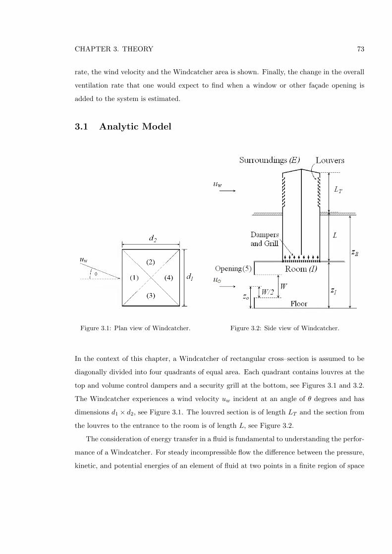
CHAPTER 3. THEORY 73
rate, the wind velocity and the Windcatcher area is shown. Finally, the change in the overall
ventilation rate that one would expect to find when a window or other facade opening is
added to the system is estimated.
3.1 Analytic Model
Figure 3.1: Plan view of Windcatcher. Figure 3.2: Side view of Windcatcher.
In the context of this chapter, a Windcatcher of rectangular cross–section is assumed to be
diagonally divided into four quadrants of equal area. Each quadrant contains louvres at the
top and volume control dampers and a security grill at the bottom, see Figures 3.1 and 3.2.
The Windcatcher experiences a wind velocity uw incident at an angle of θ degrees and has
dimensions d1 × d2, see Figure 3.1. The louvred section is of length LT and the section from
the louvres to the entrance to the room is of length L, see Figure 3.2.
The consideration of energy transfer in a fluid is fundamental to understanding the perfor-
mance of a Windcatcher. For steady incompressible flow the difference between the pressure,
kinetic, and potential energies of an element of fluid at two points in a finite region of space
CHAPTER 3. THEORY 74
(a control volume) is equal to the energy lost from the system and may be described by an
energy Equation (see Munson et al., 1998, for example). To model the performance of a
Windcatcher, conservation of energy and mass are enforced using a method similar to that
reported by Etheridge & Sandberg (1996) and CIBSE (2005a). For a quadrant that faces
into the wind, flow is from the surroundings into the room and here conservation of energy
yields (Etheridge & Sandberg, 1996)
∆pin = pE − pI −∆ρgzI + pw (3.1)
where pE is the external pressure measured at ground level immediately outside the building,
pI is the internal pressure measured at ground level inside the building, and ∆pin is the
pressure drop over the Windcatcher quadrant, and assumes that all losses between the room
and the surroundings are solely attributed to the Windcatcher. In addition, ∆ρ denotes the
change in air density between the room and the surroundings, zI is the height of the entrance
to the Windcatcher relative to the floor of the room, and pw denotes the pressure generated
by the wind. Similarly, for a quadrant in which air moves from the room to the surroundings,
∆pout = pI − pE + ∆ρgzE − pw (3.2)
where ∆pout is the pressure drop over the outlet quadrant and zE is the height of the top of
the Windcatcher relative to the floor of the room.
The pressure generated by the action of the wind over the face of a Windcatcher quadrant
is related to the velocity of the air flowing into or out of the quadrant by the coefficient of
pressure Cp, which is defined as (Etheridge & Sandberg, 1996)
Cp =∆p
ρEu2w/2
(3.3)
Here, ∆p is the difference between the static pressure on the face of the Windcatcher
(pw) and a reference pressure, and uw is the wind speed measured at Windcatcher height on
the windward side and in the free stream. So, for air that flows from the surroundings into
the room (an “inlet” quadrant) Equation (3.1) may be re–written as (Etheridge & Sandberg,
1996)
CHAPTER 3. THEORY 75
∆pin =1
2ρEu
2wCp − gzI(ρE − ρI)− pI (3.4)
where ∆ρ = ρE−ρI and the reference pressure is assumed to be atmospheric. Equation (3.4)
makes several key assumptions: the first is that the ventilation is steady, which may seem
unlikely if generated by a gusting wind, but Etheridge & Sandberg (1996) suggest that the
ventilation rate is more likely to be steady in the mean rather than being truly steady and this
is acceptable; second, the internal velocity is very small and thus negligible when compared
to the wind velocity. Finally, changes in the density of the air caused by the variation of
pressure with height may be neglected. So, for an outlet quadrant
∆pout = pI − gzE(ρI − ρE)− 1
2ρEu
2wCp (3.5)
Application of the ideal gas equation of state (p = ρRT ) to equations (3.4) and (3.5) gives
∆pin =1
2ρEu
2wCp −
gzIR
(pETE− pITI
)− pI (3.6)
and
∆pout = pI −gzER
(pITI− pETE
)− 1
2ρEu
2wCp (3.7)
However, the changes in density that appear in equations (3.4) and (3.5) are assumed to be
due solely to a change in temperature and so, following Etheridge & Sandberg (1996), an
assumption of pI = pE is made for the density components and equations (3.6) and (3.7) are
re-written as
∆pin =1
2ρEu
2wCp −
gzIpER
(1
TE− 1
TI
)− pI (3.8)
and
∆pout = pI −gzEpER
(1
TI− 1
TE
)− 1
2ρEu
2wCp (3.9)
CHAPTER 3. THEORY 76
Here, T denotes the temperature, R is the specific gas constant for air, and ∆pin and
∆pout represent the drop in pressure over the supply and extract quadrants respectively. The
losses imparted by the Windcatcher, and which cause the pressure to drop, may be expressed
in a number of ways; for example, by using a standard loss coefficient Cd (see CIBSE, 2005a).
However, the Windcatcher contains many different components and it is desirable to gain an
appreciation of how each one impacts on the overall Windcatcher performance. Therefore,
the losses are expressed in terms of a loss coefficient K, where in general
Kin,out =∆pin,out
0.5ρu2in,out
(3.10)
This allows Equations (3.8) and (3.9) to be re-written to give
1
2ρu2
inKin =1
2ρEu
2wCp −
gzIpER
(1
TE− 1
TI
)− pI (3.11)
and
1
2ρu2
outKout = pI −gzEpER
(1
TI− 1
TE
)− 1
2ρEu
2wCp (3.12)
Here, uin and uout represent the velocity inside the quadrant of an inlet and outlet quad-
rant respectively, and ρ is an average value for the density over the length of the quadrant.
For θ = 0◦, it may be assumed that one quadrant acts as an inlet [quadrant (1)] and
the remaining three quadrants act as outlets, where quadrants 2 and 3 are assumed to be
identical, see the experimental data of Elmualim (2006a) for example. After re-arranging,
the conservation of energy for each inlet and outlet quadrant may be written as
1
2ρu2
1K1 =1
2ρEu
2wCp1 −
gzIpER
(1
TE− 1
TI
)− pI (3.13)
1
2ρu2
2K2 = pI +gzEpER
(1
TE− 1
TI
)− 1
2ρEu
2wCp2 (3.14)
and
CHAPTER 3. THEORY 77
1
2ρu2
4K4 = pI +gzEpER
(1
TE− 1
TI
)− 1
2ρEu
2wCp4 (3.15)
where it is assumed that the external temperature is the same for each quadrant.
Similarly, these equations may also be used to describe energy conservation through an
opening in the facade of a room containing a Windcatcher. Purpose provided openings, such
as air vents, windows, and doors are generally characterised as sharp-edged openings with
a negligible thickness (Etheridge & Sandberg, 1996). Accordingly, a rectangular opening
located at the midpoint of the facade in both the vertical and horizontal planes is considered
here. The vertical midpoint of the opening is assumed to be at a height zO from the floor
of the room (see Fig. 3.2), and it is assumed that the air flow incident to the opening is
uniform.
The analysis of the flow through the Windcatcher follows Equations (3.11) and (3.12). For
the opening, the flow of air around the building induces a change in pressure on each facade
so that an opening with the wind incident upon it (located in the windward region) will have
a higher pressure than the room, whilst an opening located in the leeward region will have a
lower pressure because of energy dissipation through flow separation and turbulence. If the
facade opening (designated the 5th opening in Fig. 3.2) is in an area of positive pressure then
conservation of energy gives
1
2ρEu
25K5 =
1
2ρEu
2wCp5 −
gzOpER
(1
TE− 1
TI
)− pI (3.16)
and if the opening is in an area of negative pressure, then
1
2ρIu
25K5 = pI −
gzOpER
(1
TI− 1
TE
)− 1
2ρEu
2wCp5 (3.17)
Here, Cp5 is introduced as a modified loss coefficient for the facade containing the opening
and is used because it is convenient to refer the wind velocity incident at the opening back
to the wind velocity at roof height used for the Windcatcher computations in Equations
(3.13)—(3.15). This may be achieved using an appropriate correction equation to account
CHAPTER 3. THEORY 78
for the difference in height and the terrain. Accordingly, the equation of BS EN 5925 (BSI,
1991), Liddament (1996, Chapter 12), Etheridge & Sandberg (1996, Chapter 4), Santamouris
& Asimakopoulos (1996, Chapter 9), and Orme & Leksmono (2002, Section 2.2.4) is used,
although other conversion equations are available (see for example Etheridge & Sandberg,
1996, chapter 14), because it allows the velocity at roof level to be scaled using readily
available conversion constants that are based upon a knowledge of the local terrain and the
height of the building, so that
uwu10
= kzaE (3.18)
where u10 is the wind velocity measured in open country at a height of 10 m, and k and a
are topographically dependent constants where k has units m−a. Equation (3.18) may now
be re–written to form two simultaneous equations so that each accounts for the difference in
wind velocity between heights zE and zO, respectively, and are then combined to eliminate
u10 and k and give the following definition for Cp5
Cp5 = Cp5[zO/zE ]2a (3.19)
To solve Equations (3.13)—(3.17) it is necessary to enforce mass continuity, and how this
is done depends upon the conditions assumed inside the room. Here, there are two limiting
cases (i) a room in which air exchange with the surrounds is permitted, and (ii) a room that
is perfectly sealed. For an autonomous Windcatcher, both scenarios are considered, with a
sealed room studied first in Section 3.1.1, and an unsealed room studies in second in Section
3.1.2. However, when a Windcatcher is coupled with a facade opening the supplied room
can no longer be considered to be truly sealed because it is expected that air flow through
the opening will help to balance mass through the room. Furthermore, because air flow
through adventitious openings is likely to be negligible when compared to the flow through
the facade opening they may be ignored. Accordingly, a single scenario for a Windcatcher in
coordination a facade opening is considered in Section 3.1.3.
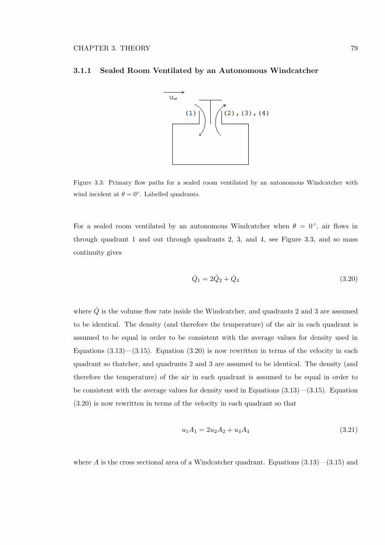
CHAPTER 3. THEORY 79
3.1.1 Sealed Room Ventilated by an Autonomous Windcatcher
Figure 3.3: Primary flow paths for a sealed room ventilated by an autonomous Windcatcher with
wind incident at θ = 0◦. Labelled quadrants.
For a sealed room ventilated by an autonomous Windcatcher when θ = 0 ◦, air flows in
through quadrant 1 and out through quadrants 2, 3, and 4, see Figure 3.3, and so mass
continuity gives
Q1 = 2Q2 + Q4 (3.20)
where Q is the volume flow rate inside the Windcatcher, and quadrants 2 and 3 are assumed
to be identical. The density (and therefore the temperature) of the air in each quadrant is
assumed to be equal in order to be consistent with the average values for density used in
Equations (3.13)—(3.15). Equation (3.20) is now rewritten in terms of the velocity in each
quadrant so thatcher, and quadrants 2 and 3 are assumed to be identical. The density (and
therefore the temperature) of the air in each quadrant is assumed to be equal in order to
be consistent with the average values for density used in Equations (3.13)—(3.15). Equation
(3.20) is now rewritten in terms of the velocity in each quadrant so that
u1A1 = 2u2A2 + u4A4 (3.21)
where A is the cross sectional area of a Windcatcher quadrant. Equations (3.13)—(3.15) and
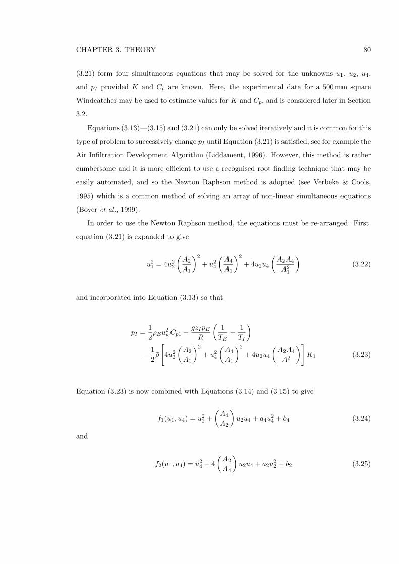
CHAPTER 3. THEORY 80
(3.21) form four simultaneous equations that may be solved for the unknowns u1, u2, u4,
and pI provided K and Cp are known. Here, the experimental data for a 500 mm square
Windcatcher may be used to estimate values for K and Cp, and is considered later in Section
3.2.
Equations (3.13)—(3.15) and (3.21) can only be solved iteratively and it is common for this
type of problem to successively change pI until Equation (3.21) is satisfied; see for example the
Air Infiltration Development Algorithm (Liddament, 1996). However, this method is rather
cumbersome and it is more efficient to use a recognised root finding technique that may be
easily automated, and so the Newton Raphson method is adopted (see Verbeke & Cools,
1995) which is a common method of solving an array of non-linear simultaneous equations
(Boyer et al., 1999).
In order to use the Newton Raphson method, the equations must be re-arranged. First,
equation (3.21) is expanded to give
u21 = 4u2
2
(A2
A1
)2
+ u24
(A4
A1
)2
+ 4u2u4
(A2A4
A21
)(3.22)
and incorporated into Equation (3.13) so that
pI =1
2ρEu
2wCp1 −
gzIpER
(1
TE− 1
TI
)−1
2ρ
[4u2
2
(A2
A1
)2
+ u24
(A4
A1
)2
+ 4u2u4
(A2A4
A21
)]K1 (3.23)
Equation (3.23) is now combined with Equations (3.14) and (3.15) to give
f1(u1, u4) = u22 +
(A4
A2
)u2u4 + a4u
24 + b4 (3.24)
and
f2(u1, u4) = u24 + 4
(A2
A4
)u2u4 + a2u
22 + b2 (3.25)
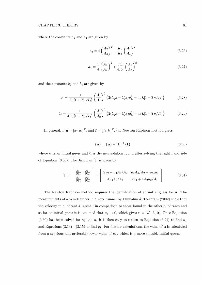
CHAPTER 3. THEORY 81
where the constants a2 and a4 are given by
a2 = 4
(A2
A4
)2
+K2
K1
(A1
A4
)2
(3.26)
a4 =1
4
(A4
A2
)2
+K4
4K1
(A1
A2
)2
(3.27)
and the constants b2 and b4 are given by
b2 =1
K1[1 + TE/TI ]
(A1
A4
)2 {2(Cp2 − Cp1)u2
w − 4gL[1− TE/TI ]}
(3.28)
b4 =1
4K1[1 + TE/TI ]
(A1
A2
)2 {2(Cp4 − Cp1)u2
w − 4gL[1− TE/TI ]}. (3.29)
In general, if u = [u2 u4]T , and f = [f1 f2]T , the Newton Raphson method gives
{u} = {u} − [J]−1 {f} (3.30)
where u is an initial guess and u is the new solution found after solving the right hand side
of Equation (3.30). The Jacobian [J] is given by
[J] =
∂f1∂u2
∂f1∂u4
∂f2∂u2
∂f2∂u4
=
2u2 + u4A4/A2 u2A4/A2 + 2a4u4
4u4A2/A4 2u4 + 4A2u2/A4
(3.31)
The Newton Raphson method requires the identification of an initial guess for u. The
measurements of a Windcatcher in a wind tunnel by Elmualim & Teekaram (2002) show that
the velocity in quadrant 4 is small in comparison to those found in the other quadrants and
so for an initial guess it is assumed that u4 → 0, which gives u = [√−b4 0]. Once Equation
(3.30) has been solved for u2 and u4 it is then easy to return to Equation (3.21) to find u1
and Equations (3.13)—(3.15) to find pI . For further calculations, the value of u is calculated
from a previous and preferably lower value of uw, which is a more suitable initial guess.
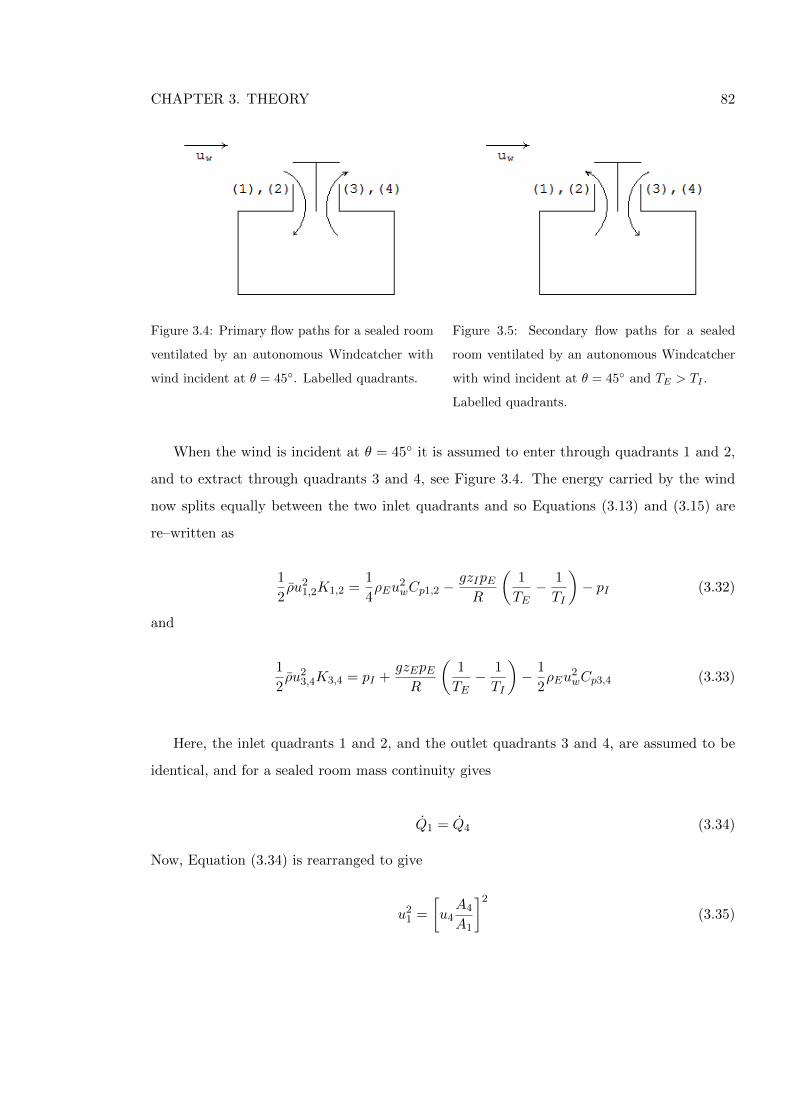
CHAPTER 3. THEORY 82
Figure 3.4: Primary flow paths for a sealed room
ventilated by an autonomous Windcatcher with
wind incident at θ = 45◦. Labelled quadrants.
Figure 3.5: Secondary flow paths for a sealed
room ventilated by an autonomous Windcatcher
with wind incident at θ = 45◦ and TE > TI .
Labelled quadrants.
When the wind is incident at θ = 45◦ it is assumed to enter through quadrants 1 and 2,
and to extract through quadrants 3 and 4, see Figure 3.4. The energy carried by the wind
now splits equally between the two inlet quadrants and so Equations (3.13) and (3.15) are
re–written as
1
2ρu2
1,2K1,2 =1
4ρEu
2wCp1,2 −
gzIpER
(1
TE− 1
TI
)− pI (3.32)
and
1
2ρu2
3,4K3,4 = pI +gzEpER
(1
TE− 1
TI
)− 1
2ρEu
2wCp3,4 (3.33)
Here, the inlet quadrants 1 and 2, and the outlet quadrants 3 and 4, are assumed to be
identical, and for a sealed room mass continuity gives
Q1 = Q4 (3.34)
Now, Equation (3.34) is rearranged to give
u21 =
[u4A4
A1
]2
(3.35)
CHAPTER 3. THEORY 83
and incorporated into Equation (3.32) so that explicit equations for flow into and out of the
Windcatcher are given by
u3 = u4 =
√√√√√u2w(Cp1 − 2Cp4) + 4gL(1− TE/TI)(K1
(A4A1
)2+K4
)(1 + TE/TI)
(3.36)
and
u1 = u2 =A4
A1
√√√√√u2w(Cp1 − 2Cp4) + 4gL(1− TE/TI)(K1
(A4A1
)2+K4
)(1 + TE/TI)
(3.37)
The numerators of Equations (3.36) and (3.37) show that the direction of the flow in quadrants
3 and 4 and 1 and 2, respectively, will reverse when the buoyancy forces exceed those generated
by the wind and when TE > TI , see Figure 3.5. Now, using the numerators of equations (3.36)
and (3.36) this reversal is shown to occur when
uw <
√4gL(TE/TI − 1)
(Cp1 − 2Cp4)(3.38)
Air is now extracted from the room through quadrants 1 and 2, and enters the room through
quadrants 3 and 4 so that the flow equations are now given by
u3 = u4 =
√√√√√4gL(TE/TI − 1)− u2w(Cp1 − 2Cp4)(
K1
(A4A1
)2+K4
)(1 + TE/TI)
(3.39)
and
u1 = u2 =A4
A1
√√√√√4gL(TE/TI − 1)− u2w(Cp1 − 2Cp4)(
K1
(A4A1
)2+K4
)(1 + TE/TI)
(3.40)
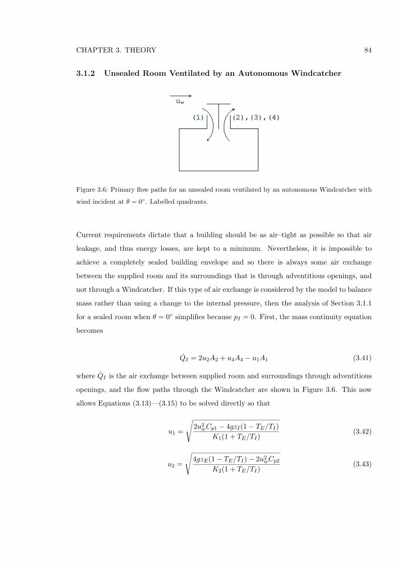
CHAPTER 3. THEORY 84
3.1.2 Unsealed Room Ventilated by an Autonomous Windcatcher
Figure 3.6: Primary flow paths for an unsealed room ventilated by an autonomous Windcatcher with
wind incident at θ = 0◦. Labelled quadrants.
Current requirements dictate that a building should be as air–tight as possible so that air
leakage, and thus energy losses, are kept to a minimum. Nevertheless, it is impossible to
achieve a completely sealed building envelope and so there is always some air exchange
between the supplied room and its surroundings that is through adventitious openings, and
not through a Windcatcher. If this type of air exchange is considered by the model to balance
mass rather than using a change to the internal pressure, then the analysis of Section 3.1.1
for a sealed room when θ = 0◦ simplifies because pI = 0. First, the mass continuity equation
becomes
QI = 2u2A2 + u4A4 − u1A1 (3.41)
where QI is the air exchange between supplied room and surroundings through adventitious
openings, and the flow paths through the Windcatcher are shown in Figure 3.6. This now
allows Equations (3.13)—(3.15) to be solved directly so that
u1 =
√2u2
wCp1 − 4gzI(1− TE/TI)
K1(1 + TE/TI)(3.42)
u2 =
√4gzE(1− TE/TI)− 2u2
wCp2
K2(1 + TE/TI)(3.43)
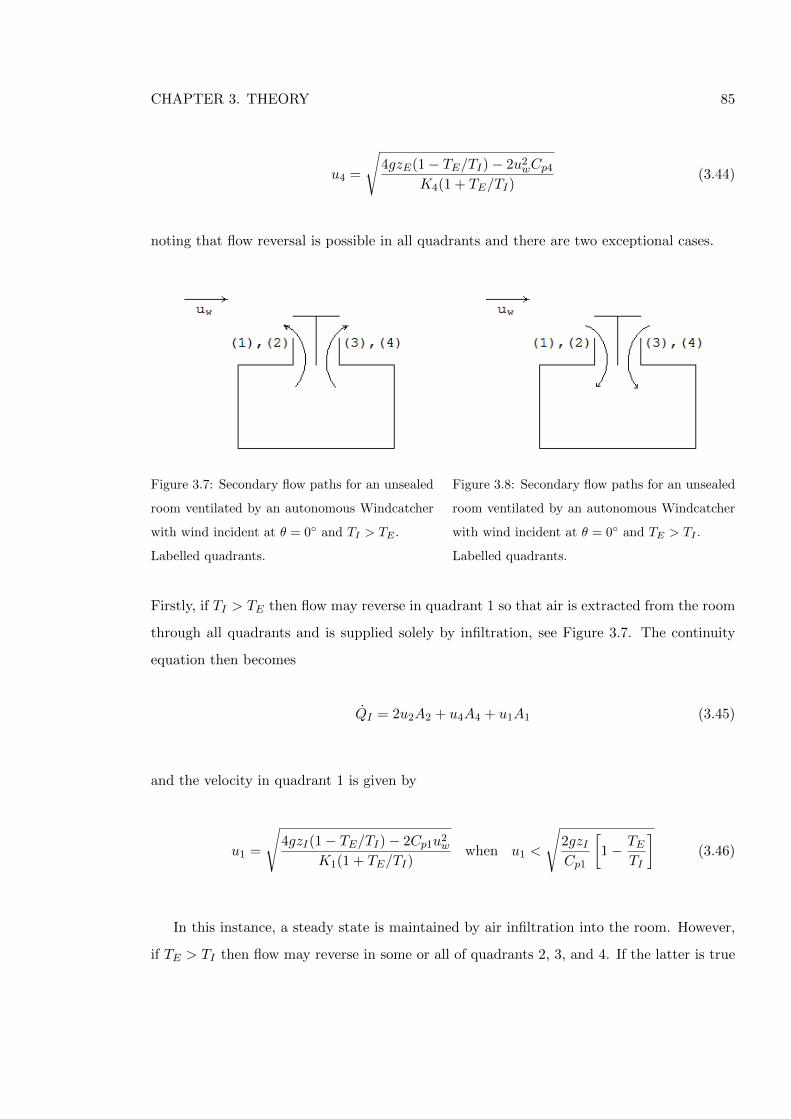
CHAPTER 3. THEORY 85
u4 =
√4gzE(1− TE/TI)− 2u2
wCp4
K4(1 + TE/TI)(3.44)
noting that flow reversal is possible in all quadrants and there are two exceptional cases.
Figure 3.7: Secondary flow paths for an unsealed
room ventilated by an autonomous Windcatcher
with wind incident at θ = 0◦ and TI > TE .
Labelled quadrants.
Figure 3.8: Secondary flow paths for an unsealed
room ventilated by an autonomous Windcatcher
with wind incident at θ = 0◦ and TE > TI .
Labelled quadrants.
Firstly, if TI > TE then flow may reverse in quadrant 1 so that air is extracted from the room
through all quadrants and is supplied solely by infiltration, see Figure 3.7. The continuity
equation then becomes
QI = 2u2A2 + u4A4 + u1A1 (3.45)
and the velocity in quadrant 1 is given by
u1 =
√4gzI(1− TE/TI)− 2Cp1u2
w
K1(1 + TE/TI)when u1 <
√2gzICp1
[1− TE
TI
](3.46)
In this instance, a steady state is maintained by air infiltration into the room. However,
if TE > TI then flow may reverse in some or all of quadrants 2, 3, and 4. If the latter is true
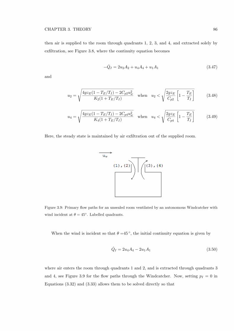
CHAPTER 3. THEORY 86
then air is supplied to the room through quadrants 1, 2, 3, and 4, and extracted solely by
exfiltration, see Figure 3.8, where the continuity equation becomes
−QI = 2u2A2 + u4A4 + u1A1 (3.47)
and
u2 =
√4gzE(1− TE/TI)− 2Cp2u2
w
K2(1 + TE/TI)when u2 <
√2gzECp2
[1− TE
TI
](3.48)
u4 =
√4gzE(1− TE/TI)− 2Cp4u2
w
K4(1 + TE/TI)when u4 <
√2gzECp4
[1− TE
TI
](3.49)
Here, the steady state is maintained by air exfiltration out of the supplied room.
Figure 3.9: Primary flow paths for an unsealed room ventilated by an autonomous Windcatcher with
wind incident at θ = 45◦. Labelled quadrants.
When the wind is incident so that θ =45 ◦, the initial continuity equation is given by
QI = 2u4A4 − 2u1A1 (3.50)
where air enters the room through quadrants 1 and 2, and is extracted through quadrants 3
and 4, see Figure 3.9 for the flow paths through the Windcatcher. Now, setting pI = 0 in
Equations (3.32) and (3.33) allows them to be solved directly so that
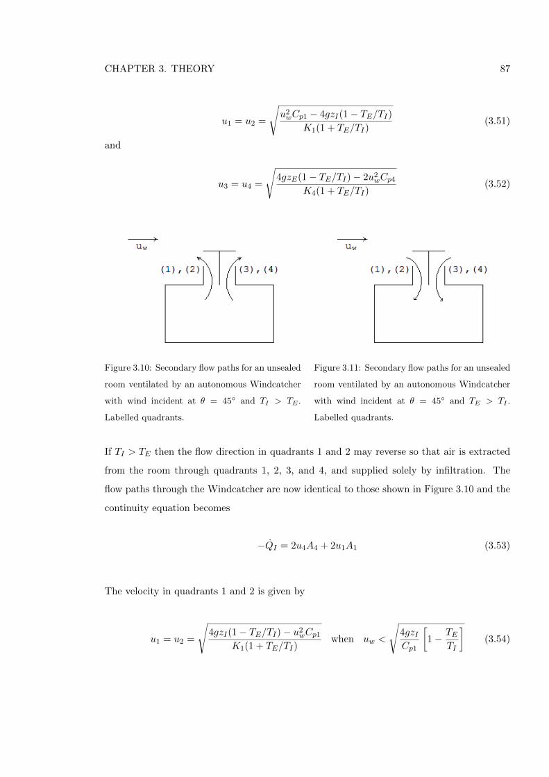
CHAPTER 3. THEORY 87
u1 = u2 =
√u2wCp1 − 4gzI(1− TE/TI)
K1(1 + TE/TI)(3.51)
and
u3 = u4 =
√4gzE(1− TE/TI)− 2u2
wCp4
K4(1 + TE/TI)(3.52)
Figure 3.10: Secondary flow paths for an unsealed
room ventilated by an autonomous Windcatcher
with wind incident at θ = 45◦ and TI > TE .
Labelled quadrants.
Figure 3.11: Secondary flow paths for an unsealed
room ventilated by an autonomous Windcatcher
with wind incident at θ = 45◦ and TE > TI .
Labelled quadrants.
If TI > TE then the flow direction in quadrants 1 and 2 may reverse so that air is extracted
from the room through quadrants 1, 2, 3, and 4, and supplied solely by infiltration. The
flow paths through the Windcatcher are now identical to those shown in Figure 3.10 and the
continuity equation becomes
−QI = 2u4A4 + 2u1A1 (3.53)
The velocity in quadrants 1 and 2 is given by
u1 = u2 =
√4gzI(1− TE/TI)− u2
wCp1
K1(1 + TE/TI)when uw <
√4gzICp1
[1− TE
TI
](3.54)
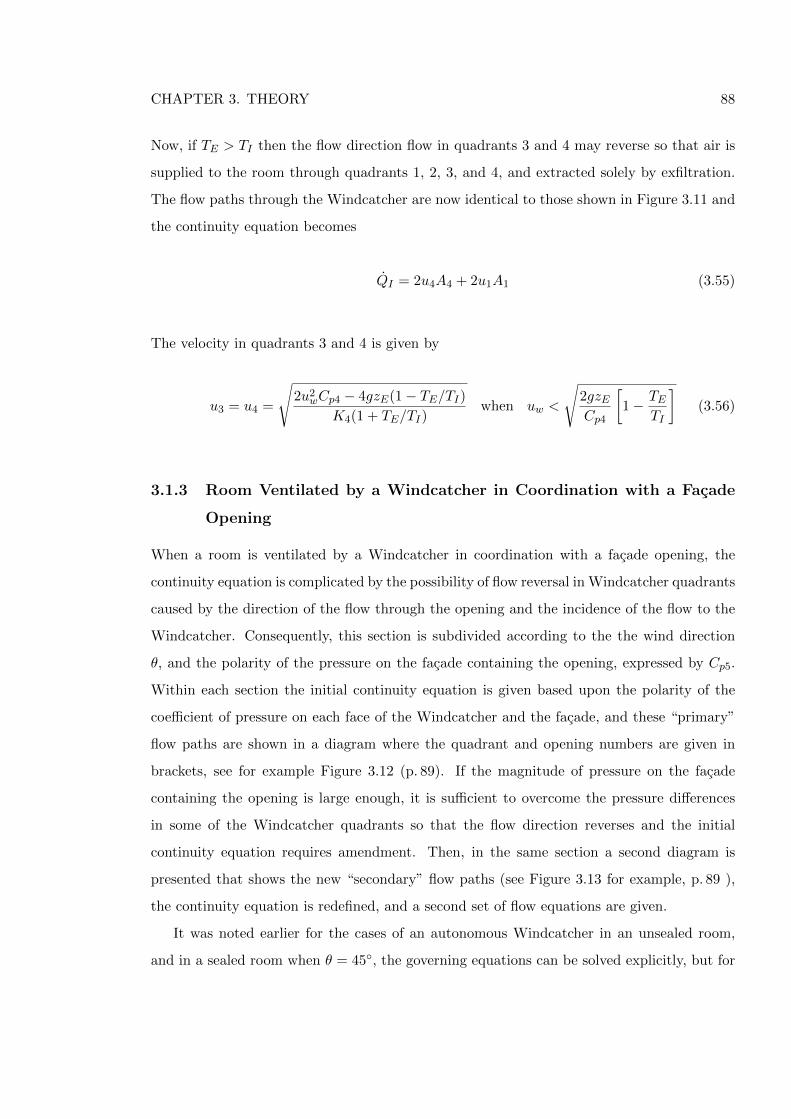
CHAPTER 3. THEORY 88
Now, if TE > TI then the flow direction flow in quadrants 3 and 4 may reverse so that air is
supplied to the room through quadrants 1, 2, 3, and 4, and extracted solely by exfiltration.
The flow paths through the Windcatcher are now identical to those shown in Figure 3.11 and
the continuity equation becomes
QI = 2u4A4 + 2u1A1 (3.55)
The velocity in quadrants 3 and 4 is given by
u3 = u4 =
√2u2
wCp4 − 4gzE(1− TE/TI)
K4(1 + TE/TI)when uw <
√2gzECp4
[1− TE
TI
](3.56)
3.1.3 Room Ventilated by a Windcatcher in Coordination with a Facade
Opening
When a room is ventilated by a Windcatcher in coordination with a facade opening, the
continuity equation is complicated by the possibility of flow reversal in Windcatcher quadrants
caused by the direction of the flow through the opening and the incidence of the flow to the
Windcatcher. Consequently, this section is subdivided according to the the wind direction
θ, and the polarity of the pressure on the facade containing the opening, expressed by Cp5.
Within each section the initial continuity equation is given based upon the polarity of the
coefficient of pressure on each face of the Windcatcher and the facade, and these “primary”
flow paths are shown in a diagram where the quadrant and opening numbers are given in
brackets, see for example Figure 3.12 (p. 89). If the magnitude of pressure on the facade
containing the opening is large enough, it is sufficient to overcome the pressure differences
in some of the Windcatcher quadrants so that the flow direction reverses and the initial
continuity equation requires amendment. Then, in the same section a second diagram is
presented that shows the new “secondary” flow paths (see Figure 3.13 for example, p. 89 ),
the continuity equation is redefined, and a second set of flow equations are given.
It was noted earlier for the cases of an autonomous Windcatcher in an unsealed room,
and in a sealed room when θ = 45◦, the governing equations can be solved explicitly, but for
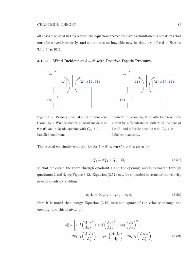
CHAPTER 3. THEORY 89
all cases discussed in this section the equations reduce to a series simultaneous equations that
must be solved iteratively, and some notes on how this may be done are offered in Section
3.1.3.5 (p. 101).
3.1.3.1 Wind Incident at θ = 0◦ with Positive Facade Pressure
Figure 3.12: Primary flow paths for a room ven-
tilated by a Windcatcher with wind incident at
θ = 0◦, and a facade opening with Cp5 > 0.
Labelled quadrants.
Figure 3.13: Secondary flow paths for a room ven-
tilated by a Windcatcher with wind incident at
θ = 0◦, and a facade opening with Cp5 > 0.
Labelled quadrants.
The typical continuity equation for for θ = 0◦ when Cp5 > 0 is given by
Q5 = 2Q2 + Q4 − Q1 (3.57)
so that air enters the room through quadrant 1 and the opening, and is extracted through
quadrants 2 and 4, see Figure 3.12. Equation (3.57) may be expanded in terms of the velocity
in each quadrant yielding
u5A5 = 2u2A3 + u4A4 − u1A1 (3.58)
Here it is noted that energy Equation (3.16) uses the square of the velocity through the
opening, and this is given by
u25 =
[4u2
1
(A1
A5
)2
+ 4u22
(A2
A5
)2
+ 4u24
(A4
A5
)2
+
2u1u2
(A1A2
A25
)− u1u4
(A1A4
A25
)− 2u2u4
(A2A4
A25
)](3.59)
CHAPTER 3. THEORY 90
Because the flow enters the room through the opening, Equation (3.16) is used to describe
the energy transfer through the opening and equated to Equation (3.13) to give
ρEu2wCp1 −
2gzIpER
(1
TE− 1
TI
)− ρu2
1K1 =
ρEu2wCp5 −
2gzOpER
(1
TE− 1
TI
)− ρEu2
5K5 (3.60)
and then re-arranged so that
u25 +
u2w
K5(Cp1 − Cp5)− 2g
K5(zI − zO)(1− TE/TI)− u2
1(1 + TE/TI)K1
2K5= 0 (3.61)
Now, by applying Equation (3.59), Equation (3.61) is rewritten to give
u22 + u2
4
1
4
(A4
A2
)2
+ u21
[A1
4A22
− (1 + TE/TI)K1
8K5
(A5
A2
)2]− u1u2
A1
2A2+ u2u4
A4
2A2
−u1u4A1A4
4A22
+
(A5
A2
)2{u2w(Cp1 − Cp5)− 2g(zI − zO)(1− TE/TI)
4K5
}= 0 (3.62)
which may be simplified to
u22 + u2
4
1
4
(A4
A2
)2
+ u21a1 − u1u2
A1
2A2+ u2u4
A4
2A2− u1u4
A1A4
4A22
+ b1 = 0 (3.63)
where the constants a1 and b1 are given by
a1 =1
4
[(A1
A2
)2
− (1 + TE/TI)K1
2K5
(A5
A2
)2]
(3.64)
b1 =
(A5
A2
)2{u2w(Cp1 − Cp5)− 2g(zI − zO)(1− TE/TI)
4K5
}(3.65)
CHAPTER 3. THEORY 91
Similarly, Equations (3.14), (3.16) and (3.59), and Equations (3.15), (3.16) and (3.59)
also combine to give
u24 + u2
1
(A1
A4
)2
+ u22a2 − u1u2
2A1A2
A24
+ u2u42A2
A4− u1u4
A1
A4+ b2 = 0 (3.66)
and
u21 + u2
2 4
(A2
A1
)2
+ u24a4 − u1u2
2A2
A1+ u2u4
2A2A4
A21
− u1u4A4
A1+ b4 = 0 (3.67)
where the constants a2, a4, b2 and b4 are given by
a2 =
[4
(A2
A4
)2
+(1 + TE/TI)K2
2K5
(A5
A4
)2]
(3.68)
a4 =
[(A4
A1
)2
+(1 + TE/TI)K4
2K5
(A5
A1
)2]
(3.69)
and
b2 =
(A5
A4
)2{u2w(Cp2 − Cp5)− 2g(zE − zO)(1− TE/TI)
K5
}(3.70)
b4 =
(A5
A1
)2{u2w(Cp4 − Cp5)− 2g(zE − zO)(1− TE/TI)
K5
}(3.71)
Equations (3.63), (3.66), and (3.67) now form three simultaneous equations that describe
the air flow through the Windcatcher and opening described by continuity Equation (3.57).
They cannot be solved explicitly, but notes on forming solutions are discussed in Section
3.1.3.5. Similar sets of equations are now derived for other values of θ, Cp5, and flow path
combinations.
If there is a high positive pressure on the facade containing the opening when θ = 0◦
and Cp5 > 0 then this may be sufficient to overcome the pressure difference in the inlet
duct (quadrant 1) of the Windcatcher, and so a secondary scenario may exist where air is
CHAPTER 3. THEORY 92
supplied to the room solely through the opening and is extracted through all quadrants of
the Windcatcher, see Figure 3.13. The new continuity equation gives
Q5 = Q1 + 2Q2 + Q4 (3.72)
Here, it is relatively straightforward to determine the conditions under which this flow
reversal will occur in quadrant 1 of the Windcatcher if the buoyancy forces are ignored in
energy Equations (3.13)—(3.16). By using each energy equation it is straightforward to show
that flow reversal will occur when
A25
K5(Cp5 − Cp1) >
[4A2
2
K2(Cp1 − Cp2) +
A24
K4(Cp1 − Cp4)
](3.73)
Consequently, Equation (3.13) now becomes
1
2ρu2
1K1 = pI +gzEpER
(1
TE− 1
TI
)− 1
2ρEu
2wCp1 (3.74)
and its combination with Equations (3.14)—(3.15) and (3.16) gives the following three simul-
taneous equations
u22 + u2
4
1
4
(A4
A2
)2
+ u21a1 + u1u2
A1
2A2+ u2u4
A4
2A2+ u1u4
A1A4
4A22
+ b1 = 0 (3.75)
u24 + u2
1
(A1
A4
)2
+ u22a2 + u1u2
2A1A2
A24
+ u2u42A2
A4+ u1u4
A1
A4+ b2 = 0 (3.76)
and
u21 + u2
2 4
(A2
A1
)2
+ u24a4 + u1u2
2A2
A1+ u2u4
2A2A4
A21
+ u1u4A4
A1+ b4 = 0 (3.77)
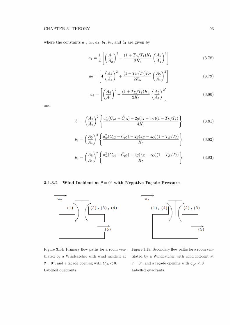
CHAPTER 3. THEORY 93
where the constants a1, a2, a4, b1, b2, and b4 are given by
a1 =1
4
[(A1
A2
)2
+(1 + TE/TI)K1
2K5
(A5
A2
)2]
(3.78)
a2 =
[4
(A2
A4
)2
+(1 + TE/TI)K2
2K5
(A5
A4
)2]
(3.79)
a4 =
[(A4
A1
)2
+(1 + TE/TI)K4
2K5
(A5
A1
)2]
(3.80)
and
b1 =
(A5
A2
)2{u2w(Cp1 − Cp5)− 2g(zI − zO)(1− TE/TI)
4K5
}(3.81)
b2 =
(A5
A4
)2{u2w(Cp2 − Cp5)− 2g(zE − zO)(1− TE/TI)
K5
}(3.82)
b4 =
(A5
A1
)2{u2w(Cp4 − Cp5)− 2g(zE − zO)(1− TE/TI)
K5
}(3.83)
3.1.3.2 Wind Incident at θ = 0◦ with Negative Facade Pressure
Figure 3.14: Primary flow paths for a room ven-
tilated by a Windcatcher with wind incident at
θ = 0◦, and a facade opening with Cp5 < 0.
Labelled quadrants.
Figure 3.15: Secondary flow paths for a room ven-
tilated by a Windcatcher with wind incident at
θ = 0◦, and a facade opening with Cp5 < 0.
Labelled quadrants.
CHAPTER 3. THEORY 94
When the wind is incident at θ = 0◦ and Cp5 < 0, the standard continuity equation is given
by
Q5 = Q1 − 2Q2 − Q4 (3.84)
so that air enters the room through quadrant 1 and is extracted through quadrants 2, 3, and
4, and the opening, see Figure 3.14. Therefore, Equations (3.13)—(3.15), (3.17) and (3.84)
combine to give the following three simultaneous equations
u22 + u2
4
1
4
(A4
A2
)2
+ u21a1 − u1u2
A1
2A2+ u2u4
A4
2A2− u1u4
A1A4
4A22
+ b1 = 0 (3.85)
u24 + u2
1
(A1
A4
)2
+ u22a2 − u1u2
2A1A2
A24
+ u2u42A2
A4− u1u4
A1
A4+ b2 = 0 (3.86)
and
u21 + u2
2 4
(A2
A1
)2
+ u24a4 − u1u2
2A2
A1+ u2u4
2A2A4
A21
− u1u4A4
A1+ b4 = 0 (3.87)
where the constants a1, a2, a4, b1, b2, and b4 are given by
a1 =1
4
[(A1
A2
)2
+(1 + TI/TE)K1
2K5
(A5
A2
)2]
(3.88)
a2 =
[4
(A2
A4
)2
− (1 + TI/TE)K2
2K5
(A5
A4
)2]
(3.89)
a4 =
[(A4
A1
)2
− (1 + TI/TE)K4
2K5
(A5
A1
)2]
(3.90)
and
b1 =
(A5
A2
)2{u2w(Cp5 − Cp1)(TI/TE) + 2g(zI − zO)(TI/TE − 1)
4K5
}(3.91)
CHAPTER 3. THEORY 95
b2 =
(A5
A4
)2{u2w(Cp5 − Cp2)(TI/TE) + 2g(zE − zO)(TI/TE − 1)
K5
}(3.92)
and
b4 =
(A5
A1
)2{u2w(Cp5 − Cp4)(TI/TE) + 2g(zE − zO)(TI/TE − 1)
K5
}(3.93)
The flow leaving the room through the opening may lower the pressure significantly to
cause the flow in quadrant 4 of the Windcatcher to reverse so that air enters the room through
quadrants 1 and 4, and is extracted through quadrants 2 and 3, and the opening, see Figure
3.15. The continuity equation is now given by
Q5 = Q1 + Q4 − 2Q2 (3.94)
By using energy Equations (3.13)—(3.15) and (3.17), flow reversal is shown to occur when
A21
K1(Cp1 − Cp4) >
[4A2
2
K2(Cp4 − Cp2) +
A25
K5(Cp4 − Cp5)
](3.95)
and Equation (3.15) is rewritten as
1
2ρu2
4K4 =1
2ρEu
2wCp4 −
gzIpER
(1
TE− 1
TI
)− pI (3.96)
which when combined with Equations (3.13)—(3.14), (3.17), and (3.94) gives the following
three simultaneous equations
u22 + u2
4
1
4
(A4
A2
)2
+ u21a1 − u1u2
A1
2A2− u2u4
A4
2A2+ u1u4
A1A4
4A22
+ b1 = 0 (3.97)
u24 + u2
1
(A1
A4
)2
+ u22a2 − u1u2
2A1A2
A24
− u2u42A2
A4+ u1u4
A1
A4+ b2 = 0 (3.98)
CHAPTER 3. THEORY 96
u21 + u2
2 4
(A2
A1
)2
+ u24a4 − u1u2
2A2
A1− u2u4
2A2A4
A21
+ u1u4A4
A1+ b4 = 0 (3.99)
where the constants a1, a2, a4, b1, b2, and b4 are given by
a1 =1
4
[(A1
A2
)2
+(1 + TI/TE)K1
2K5
(A5
A2
)2]
(3.100)
a2 =
[4
(A2
A4
)2
− (1 + TI/TE)K2
2K5
(A5
A4
)2]
(3.101)
a4 =
[(A4
A1
)2
+(1 + TI/TE)K4
2K5
(A5
A1
)2]
(3.102)
and
b1 =
(A5
A2
)2{u2w(Cp5 − Cp1)(TI/TE) + 2g(zI − zO)(TI/TE − 1)
4K5
}(3.103)
b2 =
(A5
A4
)2{u2w(Cp5 − Cp2)(TI/TE) + 2g(zE − zO)(TI/TE − 1)
K5
}(3.104)
b4 =
(A5
A1
)2{u2w(Cp5 − Cp4)(TI/TE) + 2g(zI − zO)(TI/TE − 1)
K5
}(3.105)
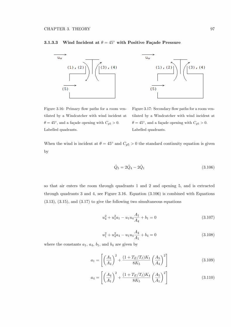
CHAPTER 3. THEORY 97
3.1.3.3 Wind Incident at θ = 45◦ with Positive Facade Pressure
Figure 3.16: Primary flow paths for a room ven-
tilated by a Windcatcher with wind incident at
θ = 45◦, and a facade opening with Cp5 > 0.
Labelled quadrants.
Figure 3.17: Secondary flow paths for a room ven-
tilated by a Windcatcher with wind incident at
θ = 45◦, and a facade opening with Cp5 > 0.
Labelled quadrants.
When the wind is incident at θ = 45◦ and Cp5 > 0 the standard continuity equation is given
by
Q5 = 2Q4 − 2Q1 (3.106)
so that air enters the room through quadrants 1 and 2 and opening 5, and is extracted
through quadrants 3 and 4, see Figure 3.16. Equation (3.106) is combined with Equations
(3.13), (3.15), and (3.17) to give the following two simultaneous equations
u24 + u2
1a1 − u1u4A1
A4+ b1 = 0 (3.107)
u21 + u2
4a4 − u1u4A4
A1+ b4 = 0 (3.108)
where the constants a1, a4, b1, and b4 are given by
a1 =
[(A1
A4
)2
+(1 + TE/TI)K1
8K5
(A5
A4
)2]
(3.109)
a4 =
[(A4
A1
)2
+(1 + TE/TI)K4
8K5
(A5
A1
)2]
(3.110)
CHAPTER 3. THEORY 98
and
b1 =
(A5
A4
)2{u2w(2Cp5 − Cp1) + 4g(zI − zO)(1− TE/TI)
8K5
}(3.111)
b4 =
(A5
A1
)2{u2w(Cp4 − Cp5)− 2g(zE − zO)(1− TE/TI)
4K5
}(3.112)
The flow entering the room through the opening may raise the pressure significantly so
as to reverse the flow in quadrants 1 and 2 of the Windcatcher so that air enters the room
through the opening and leaves through all quadrants of the Windcatcher, see Figure 3.17.
The continuity equation now gives
Q5 = 2Q4 + 2Q1 (3.113)
By using energy Equations (3.15) and (3.16) flow reversal is shown to occur when
A25
K5(2Cp5 − Cp1) >
4A24
K4(Cp1 − 2Cp4) (3.114)
and by combining Equations (3.15), (3.16), (3.74), and (3.113), the following three simulta-
neous equations are given by
u24 + u2
1a1 + u1u4A1
A4+ b1 = 0 (3.115)
u21 + u2
4a4 + u1u4A4
A1+ b4 = 0 (3.116)
where the constants a1, a4, b1, and b4 are given by
a1 =
[(A1
A4
)2
+(1 + TE/TI)K1
8K5
(A5
A4
)2]
(3.117)
a4 =
[(A4
A1
)2
+(1 + TE/TI)K4
8K5
(A5
A1
)2]
(3.118)
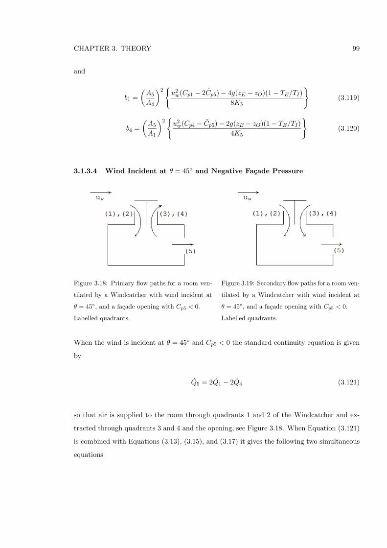
CHAPTER 3. THEORY 99
and
b1 =
(A5
A4
)2{u2w(Cp1 − 2Cp5)− 4g(zE − zO)(1− TE/TI)
8K5
}(3.119)
b4 =
(A5
A1
)2{u2w(Cp4 − Cp5)− 2g(zE − zO)(1− TE/TI)
4K5
}(3.120)
3.1.3.4 Wind Incident at θ = 45◦ and Negative Facade Pressure
Figure 3.18: Primary flow paths for a room ven-
tilated by a Windcatcher with wind incident at
θ = 45◦, and a facade opening with Cp5 < 0.
Labelled quadrants.
Figure 3.19: Secondary flow paths for a room ven-
tilated by a Windcatcher with wind incident at
θ = 45◦, and a facade opening with Cp5 < 0.
Labelled quadrants.
When the wind is incident at θ = 45◦ and Cp5 < 0 the standard continuity equation is given
by
Q5 = 2Q1 − 2Q4 (3.121)
so that air is supplied to the room through quadrants 1 and 2 of the Windcatcher and ex-
tracted through quadrants 3 and 4 and the opening, see Figure 3.18. When Equation (3.121)
is combined with Equations (3.13), (3.15), and (3.17) it gives the following two simultaneous
equations
CHAPTER 3. THEORY 100
u24 + u2
1a1 − u1u4A1
A4+ b1 = 0 (3.122)
u21 + u2
4a4 − u1u4A4
A1+ b4 = 0 (3.123)
where the constants a1, a4, b1, and b4
a1 =
[(A1
A4
)2
+(1 + TI/TE)K1
8K5
(A5
A4
)2]
(3.124)
a4 =
[(A4
A1
)2
− (1 + TI/TE)K4
8K5
(A5
A1
)2]
(3.125)
and
b1 =
(A5
A4
)2{u2w(2Cp5 − Cp1)(TI/TE) + 4g(zI − zO)(TI/TE − 1)
8K5
}(3.126)
b4 =
(A5
A1
)2{u2w(Cp5 − Cp4)(TI/TE) + 2g(zE − zO)(TI/TE − 1)
4K5
}(3.127)
The flow leaving the room through the opening may lower the pressure significantly so
as to reverse the flow in quadrant 4 of the Windcatcher so that air is supplied to the room
through all quadrants of the Windcatcher and is extracted solely through the opening, see
Figure 3.19. The continuity equation now becomes
Q5 = 2Q1 + 2Q4 (3.128)
By using Equations (3.13), (3.15), and (3.17) flow reversal is shown to occur when
A25
K5(Cp4 − Cp5) >
4A21
K1(Cp1 − 2Cp4) (3.129)
CHAPTER 3. THEORY 101
The following three simultaneous equations are now given by combining Equations (3.13),
(3.96), (3.17), and (3.128).
u24 + u2
1a1 + u1u4A1
A4+ b1 = 0 (3.130)
u21 + u2
4a4 + u1u4A4
A1+ b4 = 0 (3.131)
where the constants a1, a4, b1, and b4
a1 =
[(A1
A4
)2
+(1 + TI/TE)K1
8K5
(A5
A4
)2]
(3.132)
a4 =
[(A4
A1
)2
+(1 + TI/TE)K4
8K5
(A5
A1
)2]
(3.133)
and
b1 =
(A5
A4
)2{u2w(2Cp5 − Cp1)(TI/TE) + 4g(zI − zO)(TI/TE − 1)
8K5
}(3.134)
b4 =
(A5
A1
)2{u2w(Cp5 − Cp4)(TI/TE) + 2g(zE − zO)(TI/TE − 1)
4K5
}(3.135)
3.1.3.5 Notes on Obtaining Solutions
For the cases of an autonomous Windcatcher in an unsealed room and in a sealed room when
θ = 45◦ the equations can be solved explicitly, but for all of the other cases discussed in
this section the equations reduce to a series of two or three simultaneous equations where
implicit methodologies must be employed to derive an estimate of the flow rate through a
Windcatcher.
In Section 3.1.1, the Newton Raphson method (see Verbeke & Cools, 1995) was introduced
as a common method of solving an array of non-linear simultaneous equations (see Boyer et al.,
1999), and for the case of a Windcatcher in coordination with an opening when θ = 45◦,
equations (3.30)—(3.31) may be solved using the previously described method.
CHAPTER 3. THEORY 102
When θ = 0◦, the same method may be adapted to solve the three derived simultaneous
equations. In general, if u = [u1 u2 u4]T , and f = [f1 f2 f4]T , the Newton Raphson method
gives {u} = {u} − [J]−1 {f} where the Jacobian [J] is given by
[J] =
∂f1∂u1
∂f1∂u2
∂f1∂u4
∂f2∂u1
∂f2∂u2
∂f2∂u4
∂f4∂u1
∂f4∂u2
∂f4∂u4
(3.136)
Here, the initial guess will vary for each combination of wind incidence and facade pressure
sign, but for the case of θ = 0◦ where Cp5 > 0, the initial guess is given by u = [√−b4 0 0]
because the flow through quadrant 1 is typically significantly greater than through the other
quadrants. However, for subsequent calculations of uw, the chance of achieving convergence
is significantly increase if the previous solution is used as the next estimation.
In some instances divergence occurs and a solution cannot be found using the Newton
Raphson method, particularly when buoyancy forces are included. On these occasions an-
other iterative method can be employed; for example, a method similar to that used by the
Air Infiltration Development Algorithm (AIDA), see Orme & Leksmono (2002) and Lidda-
ment (1996) for an explanation of its capability and the code respectively. Here, the energy
equations for each Windcatcher quadrant are calculated for an initial value of pI , and the sum
of the estimated flow rates through each Windcatcher quadrant∑Q is made. The pI term
is then successively varied until∑Q = 0 and mass in and out of the Windcatcher element
balances. The accuracy of the method becomes problematic when flow reversal occurs in a
quadrant because the losses through it also change. On these occasions it may be necessary
to compute the flow rate twice, varying the loss factor each time, and collating the data
manually. Clearly then, there are computational advantages for ignoring buoyancy as well as
those previously discussed that are more scientific.
3.2 Semi–Empirical Model
The model developed in the previous Section will calculate the ventilation rates generated
by an autonomous Windcatcher or by a Windcatcher in combination with a single facade
opening provided that one knows values of Cp and K. In Section 3.2.1 the experimental
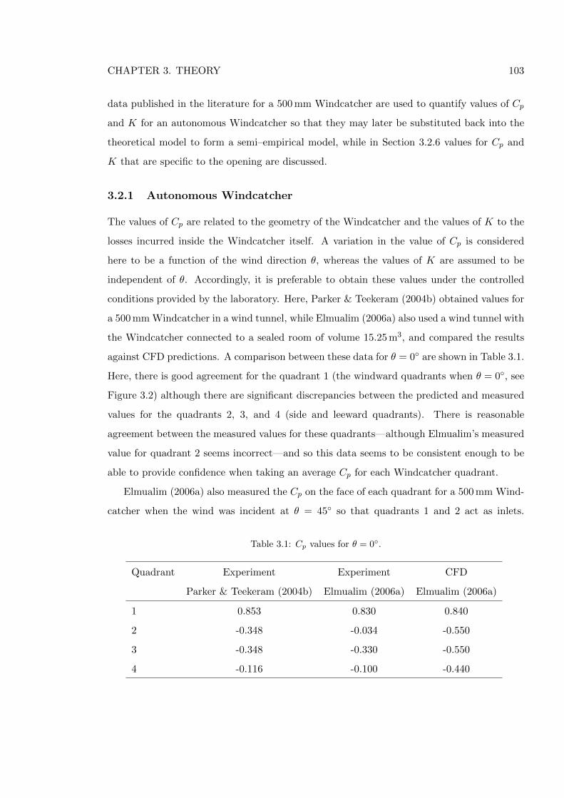
CHAPTER 3. THEORY 103
data published in the literature for a 500 mm Windcatcher are used to quantify values of Cp
and K for an autonomous Windcatcher so that they may later be substituted back into the
theoretical model to form a semi–empirical model, while in Section 3.2.6 values for Cp and
K that are specific to the opening are discussed.
3.2.1 Autonomous Windcatcher
The values of Cp are related to the geometry of the Windcatcher and the values of K to the
losses incurred inside the Windcatcher itself. A variation in the value of Cp is considered
here to be a function of the wind direction θ, whereas the values of K are assumed to be
independent of θ. Accordingly, it is preferable to obtain these values under the controlled
conditions provided by the laboratory. Here, Parker & Teekeram (2004b) obtained values for
a 500 mm Windcatcher in a wind tunnel, while Elmualim (2006a) also used a wind tunnel with
the Windcatcher connected to a sealed room of volume 15.25 m3, and compared the results
against CFD predictions. A comparison between these data for θ = 0◦ are shown in Table 3.1.
Here, there is good agreement for the quadrant 1 (the windward quadrants when θ = 0◦, see
Figure 3.2) although there are significant discrepancies between the predicted and measured
values for the quadrants 2, 3, and 4 (side and leeward quadrants). There is reasonable
agreement between the measured values for these quadrants—although Elmualim’s measured
value for quadrant 2 seems incorrect—and so this data seems to be consistent enough to be
able to provide confidence when taking an average Cp for each Windcatcher quadrant.
Elmualim (2006a) also measured the Cp on the face of each quadrant for a 500 mm Wind-
catcher when the wind was incident at θ = 45◦ so that quadrants 1 and 2 act as inlets.
Table 3.1: Cp values for θ = 0◦.
Quadrant Experiment Experiment CFD
Parker & Teekeram (2004b) Elmualim (2006a) Elmualim (2006a)
1 0.853 0.830 0.840
2 -0.348 -0.034 -0.550
3 -0.348 -0.330 -0.550
4 -0.116 -0.100 -0.440
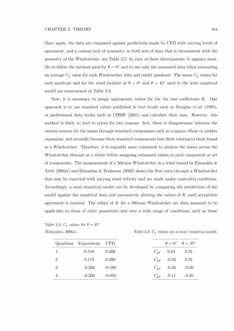
CHAPTER 3. THEORY 104
Once again, the data are compared against predictions made by CFD with varying levels of
agreement, and a curious lack of symmetry in both sets of data that is inconsistent with the
geometry of the Windcatcher, see Table 3.2. In view of these discrepancies, it appears sensi-
ble to follow the method used for θ = 0◦ and to use only the measured data when estimating
an average Cp value for each Windcatcher inlet and outlet quadrant. The mean Cp values for
each quadrant and for the wind incident at θ = 0◦ and θ = 45◦ used in the semi–empirical
model are summarised in Table 3.3.
Now, it is necessary to assign appropriate values for the the loss coefficients K. One
approach is to use standard values published in text books such as Douglas et al. (1995),
or professional data books such as CIBSE (2001) and calculate their sum. However, this
method is likely to lead to errors for two reasons: first, there is disagreement between the
various sources for the losses through standard components such as a square elbow or sudden
expansion, and secondly because these standard components bare little relation to those found
in a Windcatcher. Therefore, it is arguably more consistent to analyse the losses across the
Windcatcher element as a whole before assigning estimated values to each component or set
of components. The measurement of a 500 mm Windcatcher in a wind tunnel by Elmualim &
Awbi (2002a) and Elmualim & Teekaram (2002) shows the flow rates through a Windcatcher
that may be expected with varying wind velocity and are made under controlled conditions.
Accordingly, a semi–empirical model can be developed by comparing the predictions of the
model against the empirical data and successively altering the values of K until acceptable
agreement is reached. The values of K for a 500 mm Windcatcher are then assumed to be
applicable to those of other geometries and over a wide range of conditions, such as those
Table 3.2: Cp values for θ = 45◦
(Elmualim, 2006a).
Quadrant Experiment CFD
1 0.510 0.300
2 0.110 0.200
3 -0.200 -0.580
4 -0.200 -0.058
Table 3.3: Cp values use in semi–empirical model.
θ = 0◦ θ = 45◦
Cp1 0.84 0.31
Cp2 -0.34 0.31
Cp3 -0.34 -0.20
Cp4 -0.11 -0.20
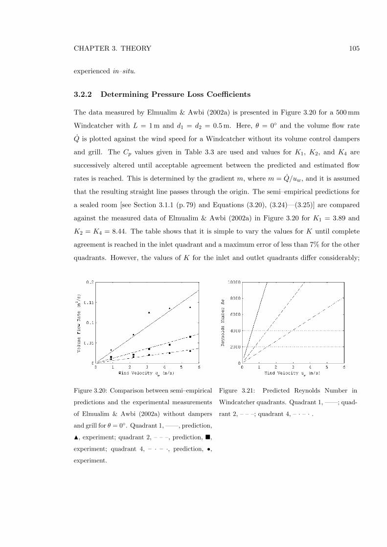
CHAPTER 3. THEORY 105
experienced in–situ.
3.2.2 Determining Pressure Loss Coefficients
The data measured by Elmualim & Awbi (2002a) is presented in Figure 3.20 for a 500 mm
Windcatcher with L = 1 m and d1 = d2 = 0.5 m. Here, θ = 0◦ and the volume flow rate
Q is plotted against the wind speed for a Windcatcher without its volume control dampers
and grill. The Cp values given in Table 3.3 are used and values for K1, K2, and K4 are
successively altered until acceptable agreement between the predicted and estimated flow
rates is reached. This is determined by the gradient m, where m = Q/uw, and it is assumed
that the resulting straight line passes through the origin. The semi–empirical predictions for
a sealed room [see Section 3.1.1 (p. 79) and Equations (3.20), (3.24)—(3.25)] are compared
against the measured data of Elmualim & Awbi (2002a) in Figure 3.20 for K1 = 3.89 and
K2 = K4 = 8.44. The table shows that it is simple to vary the values for K until complete
agreement is reached in the inlet quadrant and a maximum error of less than 7% for the other
quadrants. However, the values of K for the inlet and outlet quadrants differ considerably;
Figure 3.20: Comparison between semi–empirical
predictions and the experimental measurements
of Elmualim & Awbi (2002a) without dampers
and grill for θ = 0◦. Quadrant 1, ——, prediction,
N, experiment; quadrant 2, – – –, prediction, �,
experiment; quadrant 4, – · – ·, prediction, •,
experiment.
Figure 3.21: Predicted Reynolds Number in
Windcatcher quadrants. Quadrant 1, ——; quad-
rant 2, – – –; quadrant 4, – · – · .
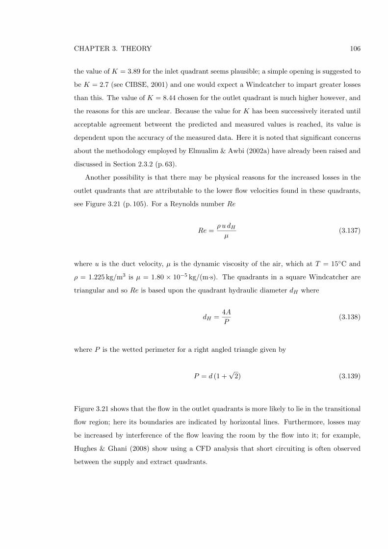
CHAPTER 3. THEORY 106
the value of K = 3.89 for the inlet quadrant seems plausible; a simple opening is suggested to
be K = 2.7 (see CIBSE, 2001) and one would expect a Windcatcher to impart greater losses
than this. The value of K = 8.44 chosen for the outlet quadrant is much higher however, and
the reasons for this are unclear. Because the value for K has been successively iterated until
acceptable agreement betweent the predicted and measured values is reached, its value is
dependent upon the accuracy of the measured data. Here it is noted that significant concerns
about the methodology employed by Elmualim & Awbi (2002a) have already been raised and
discussed in Section 2.3.2 (p. 63).
Another possibility is that there may be physical reasons for the increased losses in the
outlet quadrants that are attributable to the lower flow velocities found in these quadrants,
see Figure 3.21 (p. 105). For a Reynolds number Re
Re =ρ u dHµ
(3.137)
where u is the duct velocity, µ is the dynamic viscosity of the air, which at T = 15◦C and
ρ = 1.225 kg/m3 is µ = 1.80 × 10⁻⁵ kg/(m·s). The quadrants in a square Windcatcher are
triangular and so Re is based upon the quadrant hydraulic diameter dH where
dH =4A
P(3.138)
where P is the wetted perimeter for a right angled triangle given by
P = d (1 +√
2) (3.139)
Figure 3.21 shows that the flow in the outlet quadrants is more likely to lie in the transitional
flow region; here its boundaries are indicated by horizontal lines. Furthermore, losses may
be increased by interference of the flow leaving the room by the flow into it; for example,
Hughes & Ghani (2008) show using a CFD analysis that short circuiting is often observed
between the supply and extract quadrants.
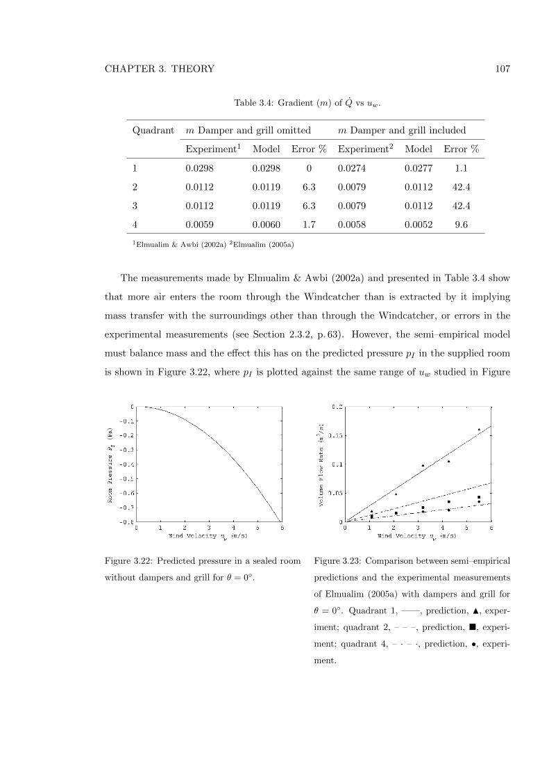
CHAPTER 3. THEORY 107
Table 3.4: Gradient (m) of Q vs uw.
Quadrant m Damper and grill omitted m Damper and grill included
Experiment1 Model Error % Experiment2 Model Error %
1 0.0298 0.0298 0 0.0274 0.0277 1.1
2 0.0112 0.0119 6.3 0.0079 0.0112 42.4
3 0.0112 0.0119 6.3 0.0079 0.0112 42.4
4 0.0059 0.0060 1.7 0.0058 0.0052 9.6
1Elmualim & Awbi (2002a) 2Elmualim (2005a)
The measurements made by Elmualim & Awbi (2002a) and presented in Table 3.4 show
that more air enters the room through the Windcatcher than is extracted by it implying
mass transfer with the surroundings other than through the Windcatcher, or errors in the
experimental measurements (see Section 2.3.2, p. 63). However, the semi–empirical model
must balance mass and the effect this has on the predicted pressure pI in the supplied room
is shown in Figure 3.22, where pI is plotted against the same range of uw studied in Figure
Figure 3.22: Predicted pressure in a sealed room
without dampers and grill for θ = 0◦.
Figure 3.23: Comparison between semi–empirical
predictions and the experimental measurements
of Elmualim (2005a) with dampers and grill for
θ = 0◦. Quadrant 1, ——, prediction, N, exper-
iment; quadrant 2, – – –, prediction, �, experi-
ment; quadrant 4, – · – ·, prediction, •, experi-
ment.
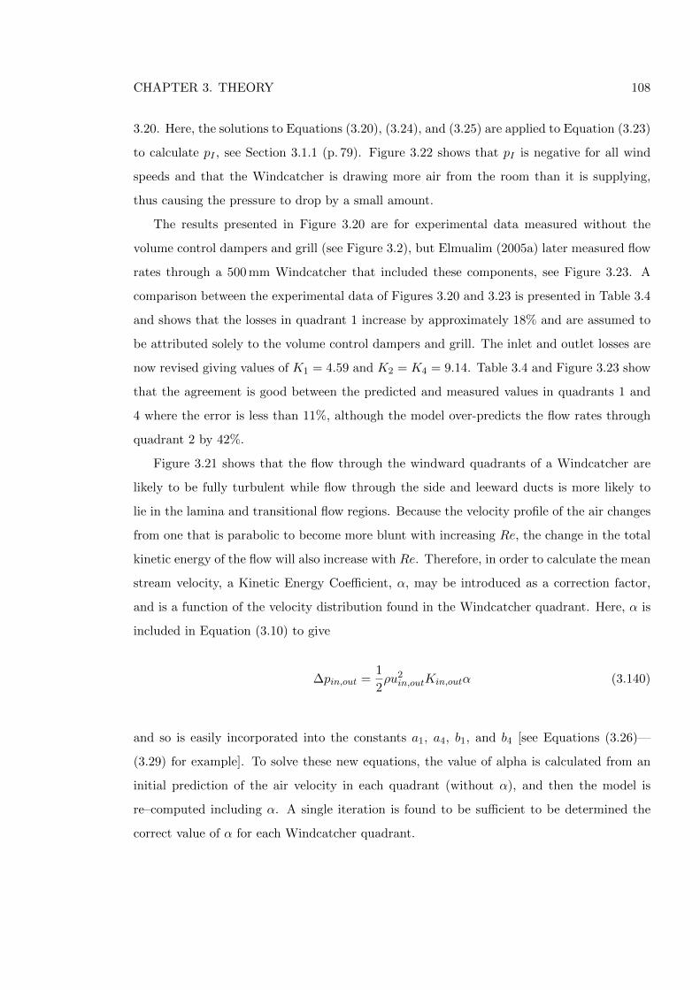
CHAPTER 3. THEORY 108
3.20. Here, the solutions to Equations (3.20), (3.24), and (3.25) are applied to Equation (3.23)
to calculate pI , see Section 3.1.1 (p. 79). Figure 3.22 shows that pI is negative for all wind
speeds and that the Windcatcher is drawing more air from the room than it is supplying,
thus causing the pressure to drop by a small amount.
The results presented in Figure 3.20 are for experimental data measured without the
volume control dampers and grill (see Figure 3.2), but Elmualim (2005a) later measured flow
rates through a 500 mm Windcatcher that included these components, see Figure 3.23. A
comparison between the experimental data of Figures 3.20 and 3.23 is presented in Table 3.4
and shows that the losses in quadrant 1 increase by approximately 18% and are assumed to
be attributed solely to the volume control dampers and grill. The inlet and outlet losses are
now revised giving values of K1 = 4.59 and K2 = K4 = 9.14. Table 3.4 and Figure 3.23 show
that the agreement is good between the predicted and measured values in quadrants 1 and
4 where the error is less than 11%, although the model over-predicts the flow rates through
quadrant 2 by 42%.
Figure 3.21 shows that the flow through the windward quadrants of a Windcatcher are
likely to be fully turbulent while flow through the side and leeward ducts is more likely to
lie in the lamina and transitional flow regions. Because the velocity profile of the air changes
from one that is parabolic to become more blunt with increasing Re, the change in the total
kinetic energy of the flow will also increase with Re. Therefore, in order to calculate the mean
stream velocity, a Kinetic Energy Coefficient, α, may be introduced as a correction factor,
and is a function of the velocity distribution found in the Windcatcher quadrant. Here, α is
included in Equation (3.10) to give
∆pin,out =1
2ρu2
in,outKin,outα (3.140)
and so is easily incorporated into the constants a1, a4, b1, and b4 [see Equations (3.26)—
(3.29) for example]. To solve these new equations, the value of alpha is calculated from an
initial prediction of the air velocity in each quadrant (without α), and then the model is
re–computed including α. A single iteration is found to be sufficient to be determined the
correct value of α for each Windcatcher quadrant.
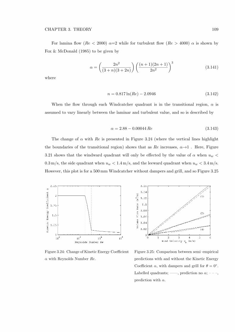
CHAPTER 3. THEORY 109
For lamina flow (Re < 2000) α=2 while for turbulent flow (Re > 4000) α is shown by
Fox & McDonald (1985) to be given by
α =
(2n2
(3 + n)(3 + 2n)
)((n+ 1)(2n+ 1)
2n2
)3
(3.141)
where
n = 0.817 ln(Re)− 2.0946 (3.142)
When the flow through each Windcatcher quadrant is in the transitional region, α is
assumed to vary linearly between the laminar and turbulent value, and so is described by
α = 2.88− 0.00044Re (3.143)
The change of α with Re is presented in Figure 3.24 (where the vertical lines highlight
the boundaries of the transitional region) shows that as Re increases, α→1 . Here, Figure
3.21 shows that the windward quadrant will only be effected by the value of α when uw <
0.3 m/s, the side quadrant when uw < 1.4 m/s, and the leeward quadrant when uw < 3.4 m/s.
However, this plot is for a 500 mm Windcatcher without dampers and grill, and so Figure 3.25
Figure 3.24: Change of Kinetic Energy Coefficient
α with Reynolds Number Re.
Figure 3.25: Comparison between semi–empirical
predictions with and without the Kinetic Energy
Coefficient α, with dampers and grill for θ = 0◦.
Labelled quadrants; ——, prediction no α; – – –,
prediction with α.
CHAPTER 3. THEORY 110
now shows the effect of applying α to the semi–empirical model for a sealed room ventilated
by a 500 mm Windcatcher, with dampers and grill. Figure 3.25 shows that including α
only has a minimal effect on the predictions of the semi–empirical model. Furthermore, this
investigation shows that it would not help to reduce the value chosen for the losses imparted
by the extract quadrants of the Windcatcher, and so it does not warrant inclusion in the
semi–empirical model presented here.
3.2.3 Identification of Component Losses
Figure 3.26: Measurements by Parker & Teekeram (2004b) of flow rate into and out of the top section
of a Windcatcher. Air flow out through quadrant, • and ——; Air flow in through quadrant, × and
– – –.
The values of loss for the inlet and outlet quadrants have been derived for the Windcatcher
as a whole and give no information on the losses attributable to individual components of the
Windcatcher apart from the estimation that the volume control dampers and grill contribute
to 18% of the total losses. Here, measurements made by Parker & Teekeram (2004b) who used
a fan to blow/draw air into and out of the top section of a 500 mm Windcatcher containing
the louvres (see Figure 3.2, p. 73) are plotted in Figure 3.26 showing the pressure drop across
the top section ∆p against the square of the volume flow rate of air Q2 through it. Here, the
losses are readily extrapolated from the gradients m obtained by linear data regression where
m = ∆p/Q2, and the Darcy–Weisbach equation (see Munson et al., 1998) for the pressure
loss over the Windcatcher section given as
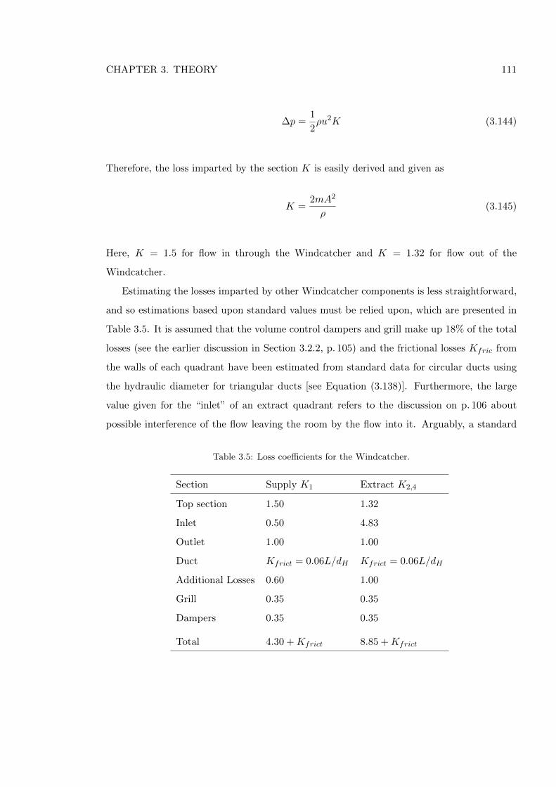
CHAPTER 3. THEORY 111
∆p =1
2ρu2K (3.144)
Therefore, the loss imparted by the section K is easily derived and given as
K =2mA2
ρ(3.145)
Here, K = 1.5 for flow in through the Windcatcher and K = 1.32 for flow out of the
Windcatcher.
Estimating the losses imparted by other Windcatcher components is less straightforward,
and so estimations based upon standard values must be relied upon, which are presented in
Table 3.5. It is assumed that the volume control dampers and grill make up 18% of the total
losses (see the earlier discussion in Section 3.2.2, p. 105) and the frictional losses Kfric from
the walls of each quadrant have been estimated from standard data for circular ducts using
the hydraulic diameter for triangular ducts [see Equation (3.138)]. Furthermore, the large
value given for the “inlet” of an extract quadrant refers to the discussion on p. 106 about
possible interference of the flow leaving the room by the flow into it. Arguably, a standard
Table 3.5: Loss coefficients for the Windcatcher.
Section Supply K1 Extract K2,4
Top section 1.50 1.32
Inlet 0.50 4.83
Outlet 1.00 1.00
Duct Kfrict = 0.06L/dH Kfrict = 0.06L/dH
Additional Losses 0.60 1.00
Grill 0.35 0.35
Dampers 0.35 0.35
Total 4.30 +Kfrict 8.85 +Kfrict
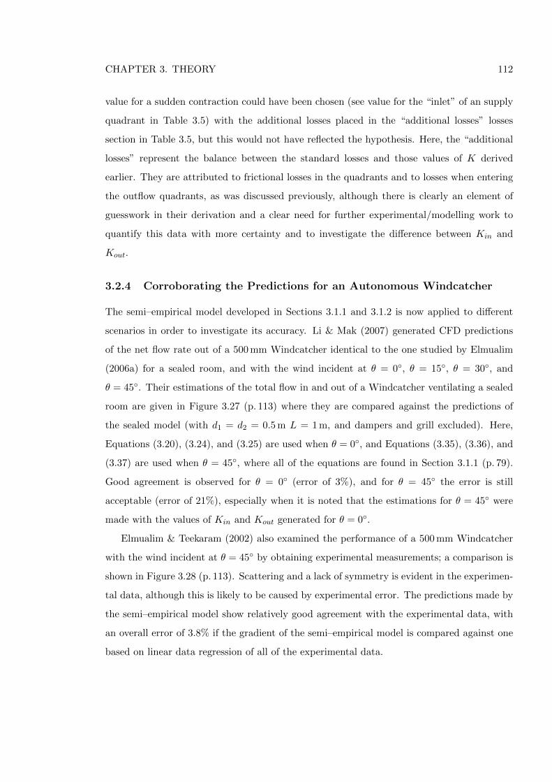
CHAPTER 3. THEORY 112
value for a sudden contraction could have been chosen (see value for the “inlet” of an supply
quadrant in Table 3.5) with the additional losses placed in the “additional losses” losses
section in Table 3.5, but this would not have reflected the hypothesis. Here, the “additional
losses” represent the balance between the standard losses and those values of K derived
earlier. They are attributed to frictional losses in the quadrants and to losses when entering
the outflow quadrants, as was discussed previously, although there is clearly an element of
guesswork in their derivation and a clear need for further experimental/modelling work to
quantify this data with more certainty and to investigate the difference between Kin and
Kout.
3.2.4 Corroborating the Predictions for an Autonomous Windcatcher
The semi–empirical model developed in Sections 3.1.1 and 3.1.2 is now applied to different
scenarios in order to investigate its accuracy. Li & Mak (2007) generated CFD predictions
of the net flow rate out of a 500 mm Windcatcher identical to the one studied by Elmualim
(2006a) for a sealed room, and with the wind incident at θ = 0◦, θ = 15◦, θ = 30◦, and
θ = 45◦. Their estimations of the total flow in and out of a Windcatcher ventilating a sealed
room are given in Figure 3.27 (p. 113) where they are compared against the predictions of
the sealed model (with d1 = d2 = 0.5 m L = 1 m, and dampers and grill excluded). Here,
Equations (3.20), (3.24), and (3.25) are used when θ = 0◦, and Equations (3.35), (3.36), and
(3.37) are used when θ = 45◦, where all of the equations are found in Section 3.1.1 (p. 79).
Good agreement is observed for θ = 0◦ (error of 3%), and for θ = 45◦ the error is still
acceptable (error of 21%), especially when it is noted that the estimations for θ = 45◦ were
made with the values of Kin and Kout generated for θ = 0◦.
Elmualim & Teekaram (2002) also examined the performance of a 500 mm Windcatcher
with the wind incident at θ = 45◦ by obtaining experimental measurements; a comparison is
shown in Figure 3.28 (p. 113). Scattering and a lack of symmetry is evident in the experimen-
tal data, although this is likely to be caused by experimental error. The predictions made by
the semi–empirical model show relatively good agreement with the experimental data, with
an overall error of 3.8% if the gradient of the semi–empirical model is compared against one
based on linear data regression of all of the experimental data.
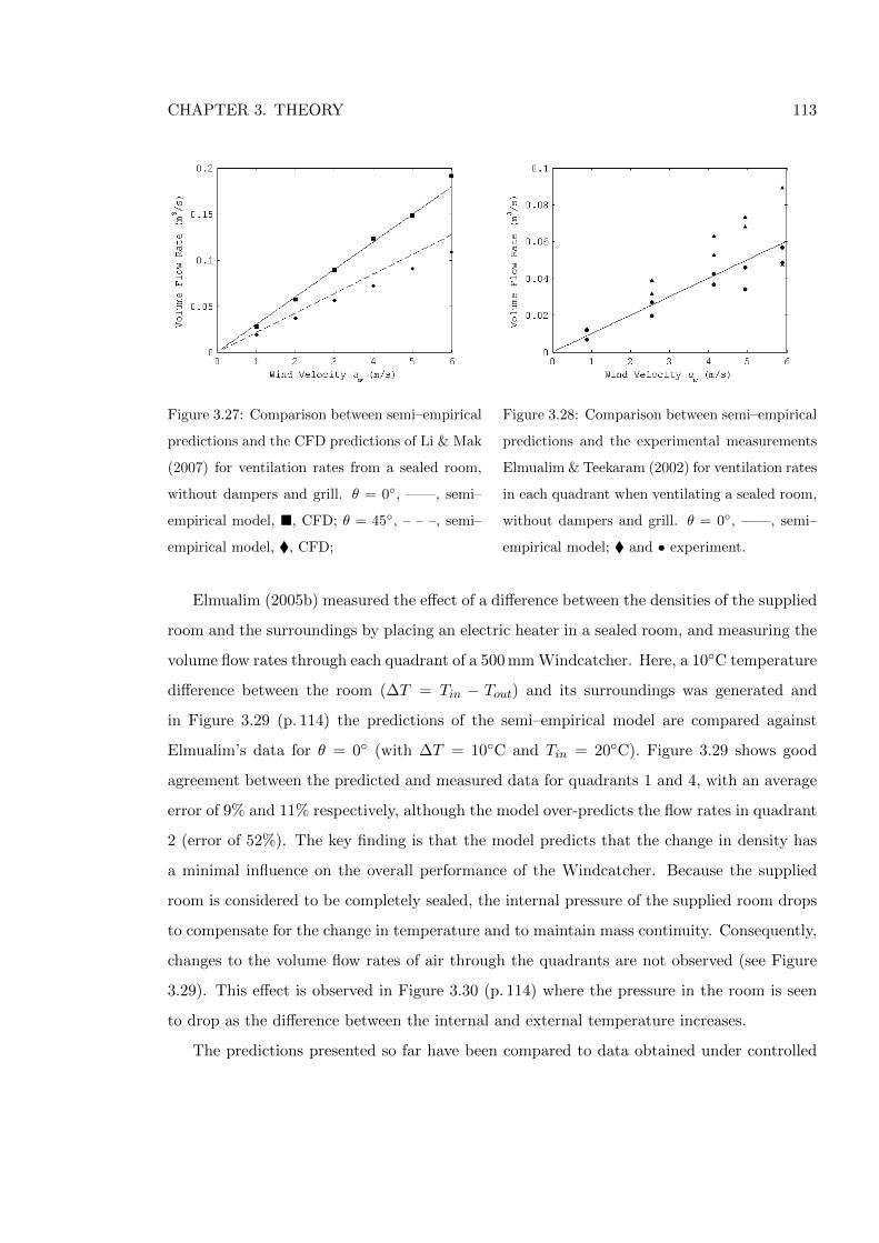
CHAPTER 3. THEORY 113
Figure 3.27: Comparison between semi–empirical
predictions and the CFD predictions of Li & Mak
(2007) for ventilation rates from a sealed room,
without dampers and grill. θ = 0◦, ——, semi–
empirical model, �, CFD; θ = 45◦, – – –, semi–
empirical model, �, CFD;
Figure 3.28: Comparison between semi–empirical
predictions and the experimental measurements
Elmualim & Teekaram (2002) for ventilation rates
in each quadrant when ventilating a sealed room,
without dampers and grill. θ = 0◦, ——, semi–
empirical model; � and • experiment.
Elmualim (2005b) measured the effect of a difference between the densities of the supplied
room and the surroundings by placing an electric heater in a sealed room, and measuring the
volume flow rates through each quadrant of a 500 mm Windcatcher. Here, a 10◦C temperature
difference between the room (∆T = Tin − Tout) and its surroundings was generated and
in Figure 3.29 (p. 114) the predictions of the semi–empirical model are compared against
Elmualim’s data for θ = 0◦ (with ∆T = 10◦C and Tin = 20◦C). Figure 3.29 shows good
agreement between the predicted and measured data for quadrants 1 and 4, with an average
error of 9% and 11% respectively, although the model over-predicts the flow rates in quadrant
2 (error of 52%). The key finding is that the model predicts that the change in density has
a minimal influence on the overall performance of the Windcatcher. Because the supplied
room is considered to be completely sealed, the internal pressure of the supplied room drops
to compensate for the change in temperature and to maintain mass continuity. Consequently,
changes to the volume flow rates of air through the quadrants are not observed (see Figure
3.29). This effect is observed in Figure 3.30 (p. 114) where the pressure in the room is seen
to drop as the difference between the internal and external temperature increases.
The predictions presented so far have been compared to data obtained under controlled
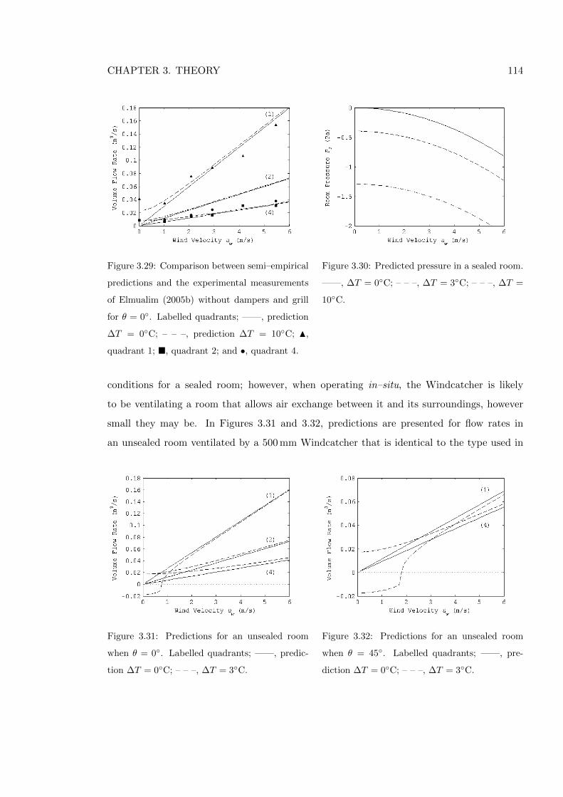
CHAPTER 3. THEORY 114
Figure 3.29: Comparison between semi–empirical
predictions and the experimental measurements
of Elmualim (2005b) without dampers and grill
for θ = 0◦. Labelled quadrants; ——, prediction
∆T = 0◦C; – – –, prediction ∆T = 10◦C; N,
quadrant 1; �, quadrant 2; and •, quadrant 4.
Figure 3.30: Predicted pressure in a sealed room.
——, ∆T = 0◦C; – – –, ∆T = 3◦C; – – –, ∆T =
10◦C.
conditions for a sealed room; however, when operating in–situ, the Windcatcher is likely
to be ventilating a room that allows air exchange between it and its surroundings, however
small they may be. In Figures 3.31 and 3.32, predictions are presented for flow rates in
an unsealed room ventilated by a 500 mm Windcatcher that is identical to the type used in
Figure 3.31: Predictions for an unsealed room
when θ = 0◦. Labelled quadrants; ——, predic-
tion ∆T = 0◦C; – – –, ∆T = 3◦C.
Figure 3.32: Predictions for an unsealed room
when θ = 45◦. Labelled quadrants; ——, pre-
diction ∆T = 0◦C; – – –, ∆T = 3◦C.
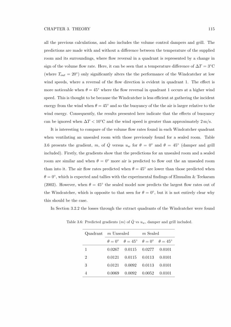
CHAPTER 3. THEORY 115
all the previous calculations, and also includes the volume control dampers and grill. The
predictions are made with and without a difference between the temperature of the supplied
room and its surroundings, where flow reversal in a quadrant is represented by a change in
sign of the volume flow rate. Here, it can be seen that a temperature difference of ∆T = 3◦C
(where Tout = 20◦) only significantly alters the the performance of the Windcatcher at low
wind speeds, where a reversal of the flow direction is evident in quadrant 1. The effect is
more noticeable when θ = 45◦ where the flow reversal in quadrant 1 occurs at a higher wind
speed. This is thought to be because the Windcatcher is less efficient at gathering the incident
energy from the wind when θ = 45◦ and so the buoyancy of the the air is larger relative to the
wind energy. Consequently, the results presented here indicate that the effects of buoyancy
can be ignored when ∆T < 10◦C and the wind speed is greater than approximately 2 m/s.
It is interesting to compare of the volume flow rates found in each Windcatcher quadrant
when ventilating an unsealed room with those previously found for a sealed room. Table
3.6 presents the gradient, m, of Q versus uw for θ = 0◦ and θ = 45◦ (damper and grill
included). Firstly, the gradients show that the predictions for an unsealed room and a sealed
room are similar and when θ = 0◦ more air is predicted to flow out the an unsealed room
than into it. The air flow rates predicted when θ = 45◦ are lower than those predicted when
θ = 0◦, which is expected and tallies with the experimental findings of Elmualim & Teekaram
(2002). However, when θ = 45◦ the sealed model now predicts the largest flow rates out of
the Windcatcher, which is opposite to that seen for θ = 0◦, but it is not entirely clear why
this should be the case.
In Section 3.2.2 the losses through the extract quadrants of the Windcatcher were found
Table 3.6: Predicted gradients (m) of Q vs uw, damper and grill included.
Quadrant m Unsealed m Sealed
θ = 0◦ θ = 45◦ θ = 0◦ θ = 45◦
1 0.0267 0.0115 0.0277 0.0101
2 0.0121 0.0115 0.0113 0.0101
3 0.0121 0.0092 0.0113 0.0101
4 0.0069 0.0092 0.0052 0.0101
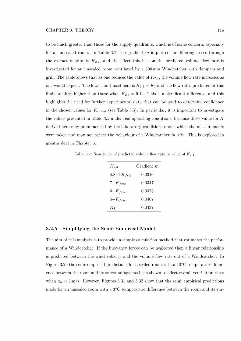
CHAPTER 3. THEORY 116
to be much greater than those for the supply quadrants, which is of some concern, especially
for an unsealed room. In Table 3.7, the gradient m is plotted for differing losses through
the extract quadrants K2,4, and the effect this has on the predicted volume flow rate is
investigated for an unsealed room ventilated by a 500 mm Windcatcher with dampers and
grill. The table shows that as one reduces the value of K2,4, the volume flow rate increases as
one would expect. The lower limit used here is K2,4 = K1 and the flow rates predicted at this
limit are 40% higher than those when K2,4 = 9.14. This is a significant difference, and this
highlights the need for further experimental data that can be used to determine confidence
in the chosen values for Kin,out (see Table 3.5). In particular, it is important to investigate
the values presented in Table 3.5 under real operating conditions, because those value for K
derived here may be influenced by the laboratory conditions under which the measurements
were taken and may not reflect the behaviour of a Windcatcher in–situ. This is explored in
greater deal in Chapter 6.
Table 3.7: Sensitivity of predicted volume flow rate to value of K2,4.
K2,4 Gradient m
8.85+Kfric 0.0310
7+Kfric 0.0347
6+Kfric 0.0373
5+Kfric 0.0407
K1 0.0437
3.2.5 Simplifying the Semi–Empirical Model
The aim of this analysis is to provide a simple calculation method that estimates the perfor-
mance of a Windcatcher. If the buoyancy forces can be neglected then a linear relationship
is predicted between the wind velocity and the volume flow rate out of a Windcatcher. In
Figure 3.29 the semi–empirical predictions for a sealed room with a 10◦C temperature differ-
ence between the room and its surroundings has been shown to effect overall ventilation rates
when uw < 1 m/s. However, Figures 3.31 and 3.32 show that the semi–empirical predictions
made for an unsealed room with a 3◦C temperature difference between the room and its sur-
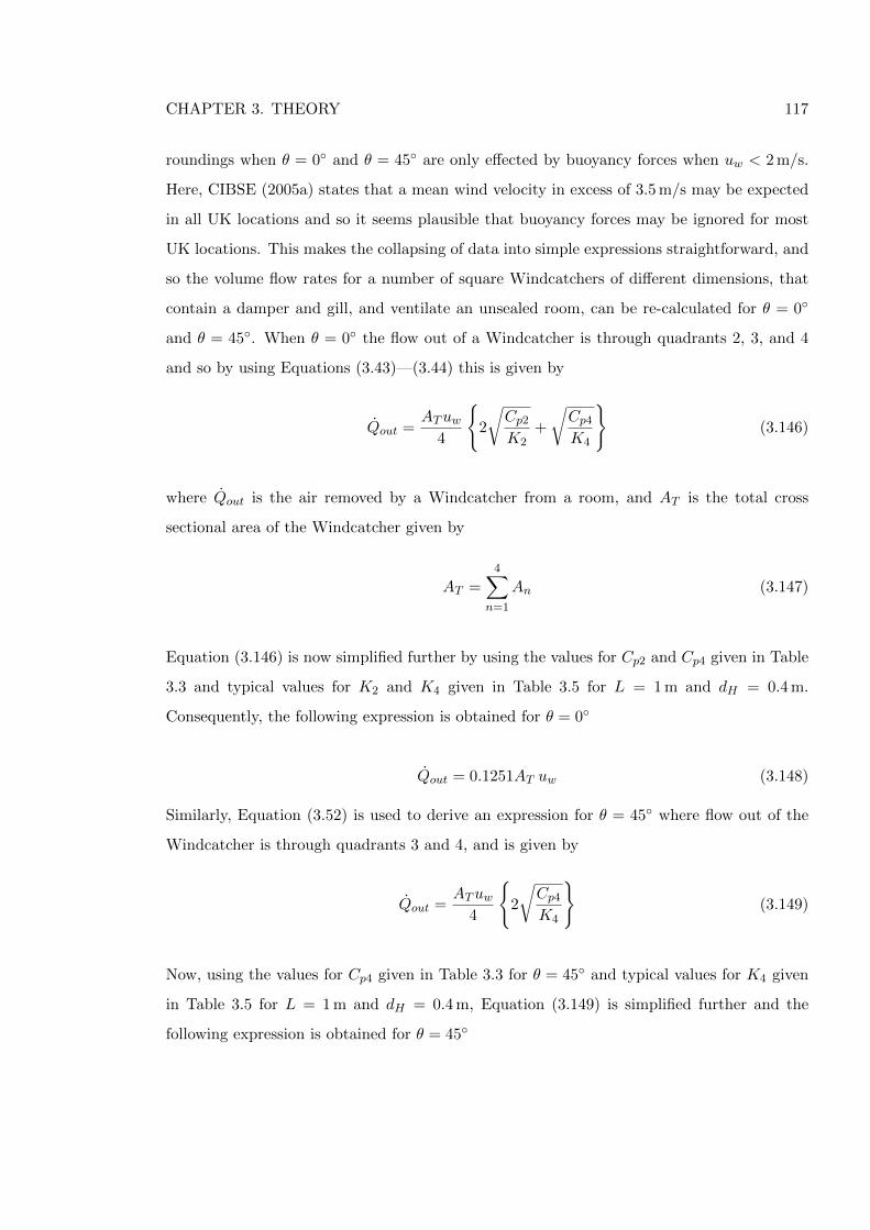
CHAPTER 3. THEORY 117
roundings when θ = 0◦ and θ = 45◦ are only effected by buoyancy forces when uw < 2 m/s.
Here, CIBSE (2005a) states that a mean wind velocity in excess of 3.5 m/s may be expected
in all UK locations and so it seems plausible that buoyancy forces may be ignored for most
UK locations. This makes the collapsing of data into simple expressions straightforward, and
so the volume flow rates for a number of square Windcatchers of different dimensions, that
contain a damper and gill, and ventilate an unsealed room, can be re-calculated for θ = 0◦
and θ = 45◦. When θ = 0◦ the flow out of a Windcatcher is through quadrants 2, 3, and 4
and so by using Equations (3.43)—(3.44) this is given by
Qout =ATuw
4
{2
√Cp2
K2+
√Cp4
K4
}(3.146)
where Qout is the air removed by a Windcatcher from a room, and AT is the total cross
sectional area of the Windcatcher given by
AT =
4∑n=1
An (3.147)
Equation (3.146) is now simplified further by using the values for Cp2 and Cp4 given in Table
3.3 and typical values for K2 and K4 given in Table 3.5 for L = 1 m and dH = 0.4 m.
Consequently, the following expression is obtained for θ = 0◦
Qout = 0.1251AT uw (3.148)
Similarly, Equation (3.52) is used to derive an expression for θ = 45◦ where flow out of the
Windcatcher is through quadrants 3 and 4, and is given by
Qout =ATuw
4
{2
√Cp4
K4
}(3.149)
Now, using the values for Cp4 given in Table 3.3 for θ = 45◦ and typical values for K4 given
in Table 3.5 for L = 1 m and dH = 0.4 m, Equation (3.149) is simplified further and the
following expression is obtained for θ = 45◦
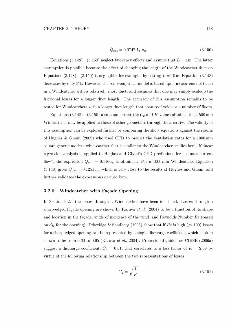
CHAPTER 3. THEORY 118
Qout = 0.0747AT uw (3.150)
Equations (3.148)—(3.150) neglect buoyancy effects and assume that L = 1 m. The latter
assumption is possible because the effect of changing the length of the Windcatcher duct on
Equations (3.148)—(3.150) is negligible; for example, by setting L = 10 m, Equation (3.148)
decreases by only 5%. However, the semi–empirical model is based upon measurements taken
in a Windcatcher with a relatively short duct, and assumes that one may simply scaleup the
frictional losses for a longer duct length. The accuracy of this assumption remains to be
tested for Windcatchers with a longer duct length that span roof voids or a number of floors.
Equations (3.148)—(3.150) also assume that the Cp and K values obtained for a 500 mm
Windcatcher may be applied to those of other geometries through the area AT . The validity of
this assumption can be explored further by comparing the short equations against the results
of Hughes & Ghani (2009) who used CFD to predict the ventilation rates for a 1000 mm
square generic modern wind-catcher that is similar to the Windcatcher studies here. If linear
regression analysis is applied to Hughes and Ghani’s CFD predictions for “counter-current
flow”, the expression Qout = 0.116uw is obtained. For a 1000 mm Windcatcher Equation
(3.148) gives Qout = 0.1251uw, which is very close to the results of Hughes and Ghani, and
further validates the expressions derived here.
3.2.6 Windcatcher with Facade Opening
In Section 3.2.1 the losses through a Windcatcher have been identified. Losses through a
sharp-edged facade opening are shown by Karava et al. (2004) to be a function of its shape
and location in the facade, angle of incidence of the wind, and Reynolds Number Re (based
on dH for the opening). Etheridge & Sandberg (1996) show that if Re is high (� 100) losses
for a sharp-edged opening can be represented by a single discharge coefficient, which is often
shown to be from 0.60 to 0.65 (Karava et al., 2004). Professional guidelines CIBSE (2006a)
suggest a discharge coefficient, Cd = 0.61, that correlates to a loss factor of K = 2.69 by
virtue of the following relationship between the two representations of losses
Cd =
√1
K(3.151)
CHAPTER 3. THEORY 119
This latter value is now used by the semi–empirical model to estimate flow through a
window while acknowledging that it is unfeasible to calculate the true losses through each
window measured in–situ, and accepting that this method may be an over simplification that
could be a source of error.
The Cp for each Windcatcher face with varying wind incidence are summarised in Table
3.3. The magnitude of Cp5 for the facade of a building is a function of the geometry of the
building, the angle of the wind incident to the facade, and the topography surrounding the
building. Estimations of Cp5 are commonly made from wind tunnel analysis, but can also be
made using predictive software (see Sawachi et al., 2006, for a discussion) or extracted from
tables. For low rise buildings of up to three storeys, Cp5 can be expressed as a mean value
for each facade of a building because the influence of the wind velocity with changing height
is relatively small. One may suggest that this assumption appears to contradict the inclusion
of Cp5 and Equation (3.19) into the model but it is argued that although the variation in
wind velocity with building height may not affect the mean Cp5 for a building facade of up to
three storeys, it will affect the wind velocity at the height of the opening significantly enough
to alter estimations of flow rate through the opening. Consequently, the sensitivity of the
semi-empirical model to its inclusion in Equation (3.19) for low rise buildings is investigated
later through a sensitivity analysis of the Cp5 parameter.
Values of Cp5 for θ = 0◦ to θ = 315◦ at intervals of θ = 45◦ are given by several sources
and Liddament (1996), Orme & Leksmono (2002), and Santamouris & Asimakopoulos (1996)
all quote similar values for buildings in a range of locations with an aspect ratio (length to
width) of 1:1 and 2:1.
The aim of this section has been to develop a semi–empirical model that can predict
ventilation rates through a room ventilated by a Windcatcher in coordination with a single
facade opening, yet there are a considerable number of unknowns. For example, there is no
guarantee that the angle of incidence of the wind on the facade will remain constant, and
so limiting values of Cp5 must be chosen so that estimations for the best and worst possible
scenarios can be made. For example, for a sheltered building of aspect 2:1 that is surrounded
by obstacles equivalent to its full height such that the aerodynamic flow fields from them
and any surrounding buildings interact, Liddament (1996) shows that the limiting values are
Cp5 = 0.06 for the windward facade and Cp5 = −0.38 for the leeward facade and are based
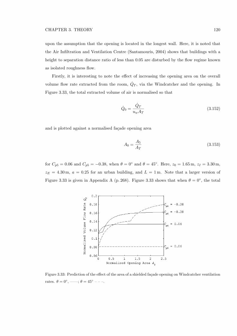
CHAPTER 3. THEORY 120
upon the assumption that the opening is located in the longest wall. Here, it is noted that
the Air Infiltration and Ventilation Centre (Santamouris, 2004) shows that buildings with a
height to separation distance ratio of less than 0.05 are disturbed by the flow regime known
as isolated roughness flow.
Firstly, it is interesting to note the effect of increasing the opening area on the overall
volume flow rate extracted from the room, QT , via the Windcatcher and the opening. In
Figure 3.33, the total extracted volume of air is normalised so that
Q0 =QT
uwAT(3.152)
and is plotted against a normalised facade opening area
A0 =A5
AT(3.153)
for Cp5 = 0.06 and Cp5 = −0.38, when θ = 0◦ and θ = 45◦. Here, z0 = 1.65 m, zI = 3.30 m,
zE = 4.30 m, a = 0.25 for an urban building, and L = 1 m. Note that a larger version of
Figure 3.33 is given in Appendix A (p. 268). Figure 3.33 shows that when θ = 0◦, the total
Figure 3.33: Prediction of the effect of the area of a shielded facade opening on Windcatcher ventilation
rates. θ = 0◦, ——; θ = 45◦ – – –.
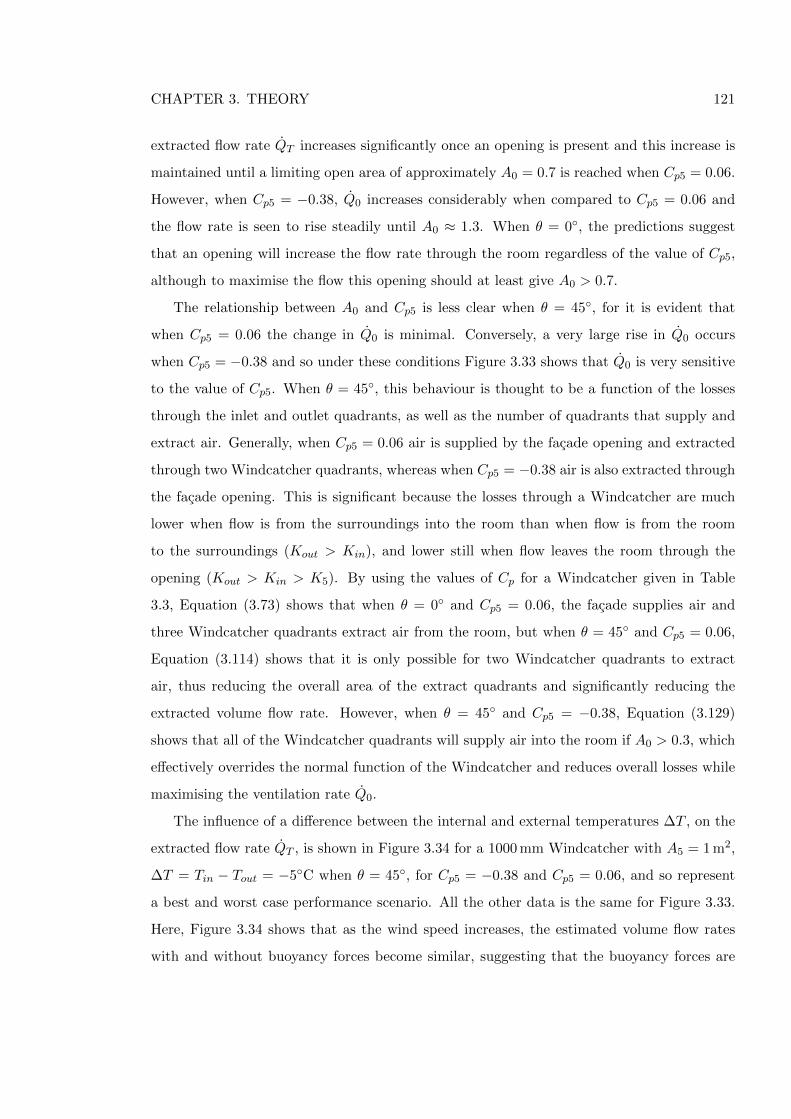
CHAPTER 3. THEORY 121
extracted flow rate QT increases significantly once an opening is present and this increase is
maintained until a limiting open area of approximately A0 = 0.7 is reached when Cp5 = 0.06.
However, when Cp5 = −0.38, Q0 increases considerably when compared to Cp5 = 0.06 and
the flow rate is seen to rise steadily until A0 ≈ 1.3. When θ = 0◦, the predictions suggest
that an opening will increase the flow rate through the room regardless of the value of Cp5,
although to maximise the flow this opening should at least give A0 > 0.7.
The relationship between A0 and Cp5 is less clear when θ = 45◦, for it is evident that
when Cp5 = 0.06 the change in Q0 is minimal. Conversely, a very large rise in Q0 occurs
when Cp5 = −0.38 and so under these conditions Figure 3.33 shows that Q0 is very sensitive
to the value of Cp5. When θ = 45◦, this behaviour is thought to be a function of the losses
through the inlet and outlet quadrants, as well as the number of quadrants that supply and
extract air. Generally, when Cp5 = 0.06 air is supplied by the facade opening and extracted
through two Windcatcher quadrants, whereas when Cp5 = −0.38 air is also extracted through
the facade opening. This is significant because the losses through a Windcatcher are much
lower when flow is from the surroundings into the room than when flow is from the room
to the surroundings (Kout > Kin), and lower still when flow leaves the room through the
opening (Kout > Kin > K5). By using the values of Cp for a Windcatcher given in Table
3.3, Equation (3.73) shows that when θ = 0◦ and Cp5 = 0.06, the facade supplies air and
three Windcatcher quadrants extract air from the room, but when θ = 45◦ and Cp5 = 0.06,
Equation (3.114) shows that it is only possible for two Windcatcher quadrants to extract
air, thus reducing the overall area of the extract quadrants and significantly reducing the
extracted volume flow rate. However, when θ = 45◦ and Cp5 = −0.38, Equation (3.129)
shows that all of the Windcatcher quadrants will supply air into the room if A0 > 0.3, which
effectively overrides the normal function of the Windcatcher and reduces overall losses while
maximising the ventilation rate Q0.
The influence of a difference between the internal and external temperatures ∆T , on the
extracted flow rate QT , is shown in Figure 3.34 for a 1000 mm Windcatcher with A5 = 1 m2,
∆T = Tin − Tout = −5◦C when θ = 45◦, for Cp5 = −0.38 and Cp5 = 0.06, and so represent
a best and worst case performance scenario. All the other data is the same for Figure 3.33.
Here, Figure 3.34 shows that as the wind speed increases, the estimated volume flow rates
with and without buoyancy forces become similar, suggesting that the buoyancy forces are
CHAPTER 3. THEORY 122
Figure 3.34: Prediction of ventilation rates for a 1000 mm Windcatcher with A5 = 1 m2 and θ = 45◦.
——, ∆T = 0◦C and Cp5 = −0.38; – – –, ∆T = 0◦C and Cp5 = 0.06; · · · · · · , ∆T = −5◦C and
Cp5 = −0.38; — · — ·, ∆T = −5◦C and Cp5 = 0.06.
only an important consideration at low wind velocity. This finding is also similar to those
for an autonomous Windcatcher, where the effect of the buoyancy forces is found only to be
significant when uw < 2m/s.
The accuracy of the prediction for a room ventilated by a Windcatcher in coordination
with a facade opening are dependent upon the choices of value for K5 and Cp5. Here, varying
K5 by ±10% had no discernible effect on the predicted ventilation rates, suggesting that inac-
curacies in this value will not have significant consequences for the behaviour observed here.
The variable Cp5 contains two constants, a and Cp5. Of these, Cp5 is the most problematic,
and Figure 3.35 (p. 123) shows the affect of varying its value for three different opening areas
A5, when θ = 45◦. The plot is asymmetric because the losses in the inlet and outlet quadrants
are dissimilar (as discussed earlier), and so the model predicts greater ventilation rates when
the opening is placed in an area of negative pressure. Initially this does not seem to agree
with the CFD predictions of Su et al. (2008) who show that when a circular Windcatcher is
mounted on the apex of a 30◦ pitched roof on an exposed square building, the opening located
on the windward facade delivers the greatest ventilation rates through the supplied room.
However, the critical factor here is that Su et al. (2008) examine an exposed building, and
Liddament (1996) reports that the windward facade has the greatest magnitude of Cp5, where
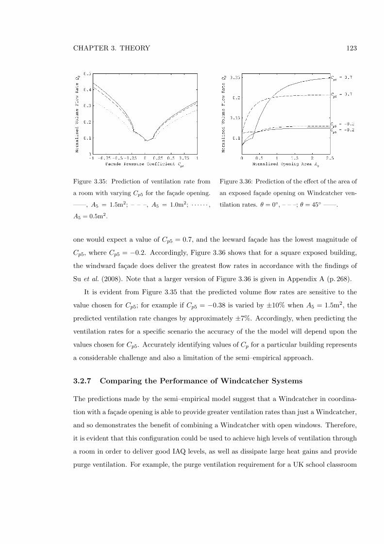
CHAPTER 3. THEORY 123
Figure 3.35: Prediction of ventilation rate from
a room with varying Cp5 for the facade opening.
——, A5 = 1.5m2; – – –, A5 = 1.0m2; · · · · · · ,
A5 = 0.5m2.
Figure 3.36: Prediction of the effect of the area of
an exposed facade opening on Windcatcher ven-
tilation rates. θ = 0◦, – – –; θ = 45◦ ——.
one would expect a value of Cp5 = 0.7, and the leeward facade has the lowest magnitude of
Cp5, where Cp5 = −0.2. Accordingly, Figure 3.36 shows that for a square exposed building,
the windward facade does deliver the greatest flow rates in accordance with the findings of
Su et al. (2008). Note that a larger version of Figure 3.36 is given in Appendix A (p. 268).
It is evident from Figure 3.35 that the predicted volume flow rates are sensitive to the
value chosen for Cp5; for example if Cp5 = −0.38 is varied by ±10% when A5 = 1.5m2, the
predicted ventilation rate changes by approximately ±7%. Accordingly, when predicting the
ventilation rates for a specific scenario the accuracy of the the model will depend upon the
values chosen for Cp5. Accurately identifying values of Cp for a particular building represents
a considerable challenge and also a limitation of the semi–empirical approach.
3.2.7 Comparing the Performance of Windcatcher Systems
The predictions made by the semi–empirical model suggest that a Windcatcher in coordina-
tion with a facade opening is able to provide greater ventilation rates than just a Windcatcher,
and so demonstrates the benefit of combining a Windcatcher with open windows. Therefore,
it is evident that this configuration could be used to achieve high levels of ventilation through
a room in order to deliver good IAQ levels, as well as dissipate large heat gains and provide
purge ventilation. For example, the purge ventilation requirement for a UK school classroom
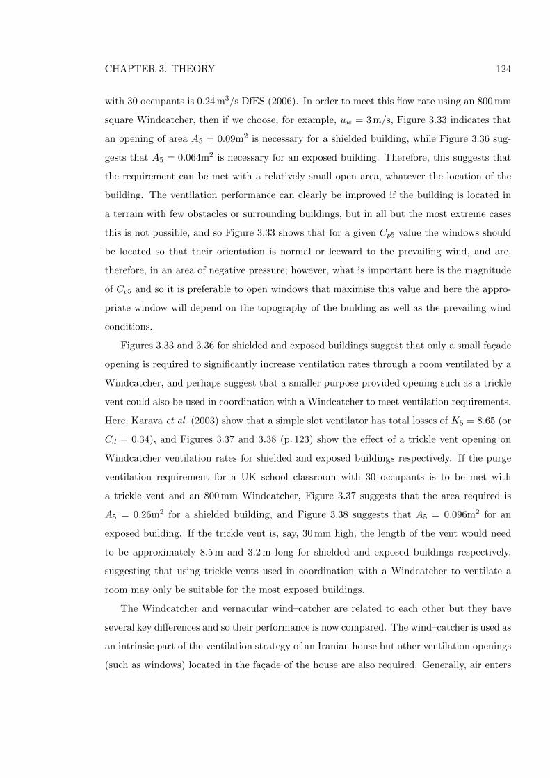
CHAPTER 3. THEORY 124
with 30 occupants is 0.24 m3/s DfES (2006). In order to meet this flow rate using an 800 mm
square Windcatcher, then if we choose, for example, uw = 3 m/s, Figure 3.33 indicates that
an opening of area A5 = 0.09m2 is necessary for a shielded building, while Figure 3.36 sug-
gests that A5 = 0.064m2 is necessary for an exposed building. Therefore, this suggests that
the requirement can be met with a relatively small open area, whatever the location of the
building. The ventilation performance can clearly be improved if the building is located in
a terrain with few obstacles or surrounding buildings, but in all but the most extreme cases
this is not possible, and so Figure 3.33 shows that for a given Cp5 value the windows should
be located so that their orientation is normal or leeward to the prevailing wind, and are,
therefore, in an area of negative pressure; however, what is important here is the magnitude
of Cp5 and so it is preferable to open windows that maximise this value and here the appro-
priate window will depend on the topography of the building as well as the prevailing wind
conditions.
Figures 3.33 and 3.36 for shielded and exposed buildings suggest that only a small facade
opening is required to significantly increase ventilation rates through a room ventilated by a
Windcatcher, and perhaps suggest that a smaller purpose provided opening such as a trickle
vent could also be used in coordination with a Windcatcher to meet ventilation requirements.
Here, Karava et al. (2003) show that a simple slot ventilator has total losses of K5 = 8.65 (or
Cd = 0.34), and Figures 3.37 and 3.38 (p. 123) show the effect of a trickle vent opening on
Windcatcher ventilation rates for shielded and exposed buildings respectively. If the purge
ventilation requirement for a UK school classroom with 30 occupants is to be met with
a trickle vent and an 800 mm Windcatcher, Figure 3.37 suggests that the area required is
A5 = 0.26m2 for a shielded building, and Figure 3.38 suggests that A5 = 0.096m2 for an
exposed building. If the trickle vent is, say, 30 mm high, the length of the vent would need
to be approximately 8.5 m and 3.2 m long for shielded and exposed buildings respectively,
suggesting that using trickle vents used in coordination with a Windcatcher to ventilate a
room may only be suitable for the most exposed buildings.
The Windcatcher and vernacular wind–catcher are related to each other but they have
several key differences and so their performance is now compared. The wind–catcher is used as
an intrinsic part of the ventilation strategy of an Iranian house but other ventilation openings
(such as windows) located in the facade of the house are also required. Generally, air enters
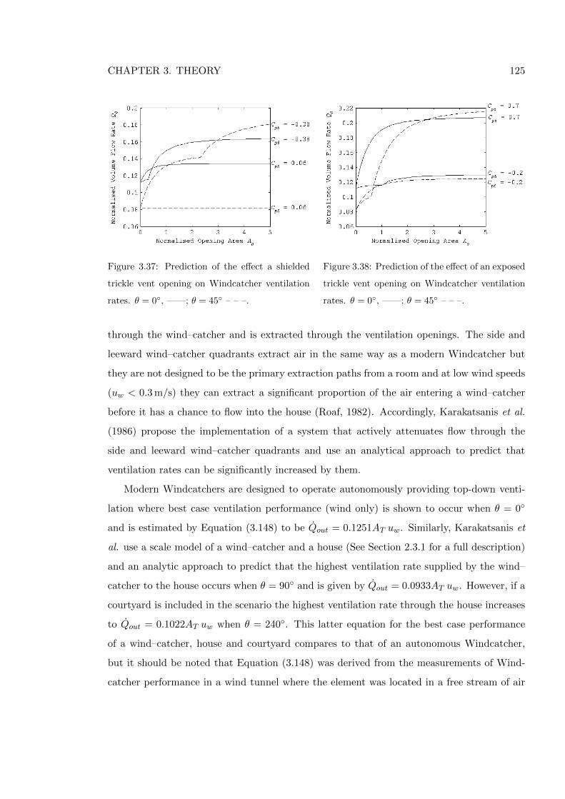
CHAPTER 3. THEORY 125
Figure 3.37: Prediction of the effect a shielded
trickle vent opening on Windcatcher ventilation
rates. θ = 0◦, ——; θ = 45◦ – – –.
Figure 3.38: Prediction of the effect of an exposed
trickle vent opening on Windcatcher ventilation
rates. θ = 0◦, ——; θ = 45◦ – – –.
through the wind–catcher and is extracted through the ventilation openings. The side and
leeward wind–catcher quadrants extract air in the same way as a modern Windcatcher but
they are not designed to be the primary extraction paths from a room and at low wind speeds
(uw < 0.3 m/s) they can extract a significant proportion of the air entering a wind–catcher
before it has a chance to flow into the house (Roaf, 1982). Accordingly, Karakatsanis et al.
(1986) propose the implementation of a system that actively attenuates flow through the
side and leeward wind–catcher quadrants and use an analytical approach to predict that
ventilation rates can be significantly increased by them.
Modern Windcatchers are designed to operate autonomously providing top-down venti-
lation where best case ventilation performance (wind only) is shown to occur when θ = 0◦
and is estimated by Equation (3.148) to be Qout = 0.1251AT uw. Similarly, Karakatsanis et
al. use a scale model of a wind–catcher and a house (See Section 2.3.1 for a full description)
and an analytic approach to predict that the highest ventilation rate supplied by the wind–
catcher to the house occurs when θ = 90◦ and is given by Qout = 0.0933AT uw. However, if a
courtyard is included in the scenario the highest ventilation rate through the house increases
to Qout = 0.1022AT uw when θ = 240◦. This latter equation for the best case performance
of a wind–catcher, house and courtyard compares to that of an autonomous Windcatcher,
but it should be noted that Equation (3.148) was derived from the measurements of Wind-
catcher performance in a wind tunnel where the element was located in a free stream of air
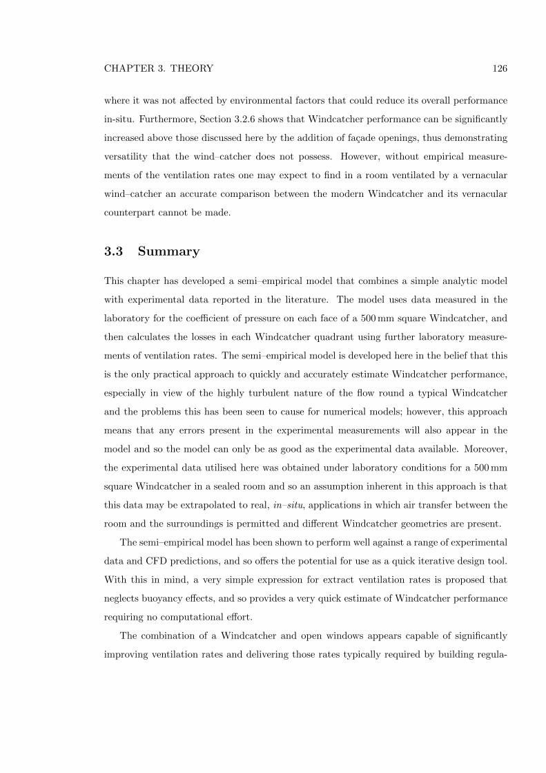
CHAPTER 3. THEORY 126
where it was not affected by environmental factors that could reduce its overall performance
in-situ. Furthermore, Section 3.2.6 shows that Windcatcher performance can be significantly
increased above those discussed here by the addition of facade openings, thus demonstrating
versatility that the wind–catcher does not possess. However, without empirical measure-
ments of the ventilation rates one may expect to find in a room ventilated by a vernacular
wind–catcher an accurate comparison between the modern Windcatcher and its vernacular
counterpart cannot be made.
3.3 Summary
This chapter has developed a semi–empirical model that combines a simple analytic model
with experimental data reported in the literature. The model uses data measured in the
laboratory for the coefficient of pressure on each face of a 500 mm square Windcatcher, and
then calculates the losses in each Windcatcher quadrant using further laboratory measure-
ments of ventilation rates. The semi–empirical model is developed here in the belief that this
is the only practical approach to quickly and accurately estimate Windcatcher performance,
especially in view of the highly turbulent nature of the flow round a typical Windcatcher
and the problems this has been seen to cause for numerical models; however, this approach
means that any errors present in the experimental measurements will also appear in the
model and so the model can only be as good as the experimental data available. Moreover,
the experimental data utilised here was obtained under laboratory conditions for a 500 mm
square Windcatcher in a sealed room and so an assumption inherent in this approach is that
this data may be extrapolated to real, in–situ, applications in which air transfer between the
room and the surroundings is permitted and different Windcatcher geometries are present.
The semi–empirical model has been shown to perform well against a range of experimental
data and CFD predictions, and so offers the potential for use as a quick iterative design tool.
With this in mind, a very simple expression for extract ventilation rates is proposed that
neglects buoyancy effects, and so provides a very quick estimate of Windcatcher performance
requiring no computational effort.
The combination of a Windcatcher and open windows appears capable of significantly
improving ventilation rates and delivering those rates typically required by building regula-
CHAPTER 3. THEORY 127
tions in the UK, although the semi–empirical model for a Windcatcher in coordination with a
facade opening has not been corroborated against data measured in–situ, and this represents
a significant knowledge gap. Accordingly, the semi–empirical model must be corroborated
against quantitative data for a Windcatcher in coordination with a facade opening in–situ
before the accuracy of its performance can be ascertained. This is done in Chapter 6.
CHAPTER 4. CASE STUDIES 128
Chapter 4
Case Studies
In this Chapter, seven schools and twenty four classrooms ventilated by a single Windcatcher
are examined. Parameters relevant to the study of the schools, classrooms, and the perfor-
mance of the Windcatcher that ventilate them are examined in detail in Sections 4.1—4.3. In
addition, a methodology to measure the performance of the Windcatcher based ventilation
strategies is explored in Section 4.4.
4.1 School Buildings
Seven schools have been chosen to test the performance of a Windcatcher based upon a
number of beneficial criteria. The choice of a suitable school building is important because
their study must give an indication of the performance of a Windcatcher in–situ, where the
performance criteria are set by the relevant UK government guidelines for indoor air quality
(IAQ) (DfES, 2006; ODPM, 2006), ventilation (DfES, 2006), and noise (DfES, 2003). All of
the schools have a number of self–contained rooms that may be categorised as purpose pro-
vided classrooms. Each classroom contains a single roof–mounted Windcatcher element that
is free from obvious shielding, obstacles, or architectural features at roof level. In addition,
none of the classrooms incorporate supplementary mechanical supply or extract ventilation.
Because of the highlighted difference in the performance of various geometries of Windcatcher
(see Elmualim & Awbi, 2002a), the greater understanding of square Windcatchers, and the
semi–empirical model of a square Windcatcher developed in Chapter 3, the majority of Wind-
catcher elements evaluated here are square. Pegg (2008) suggests that a sensible time between
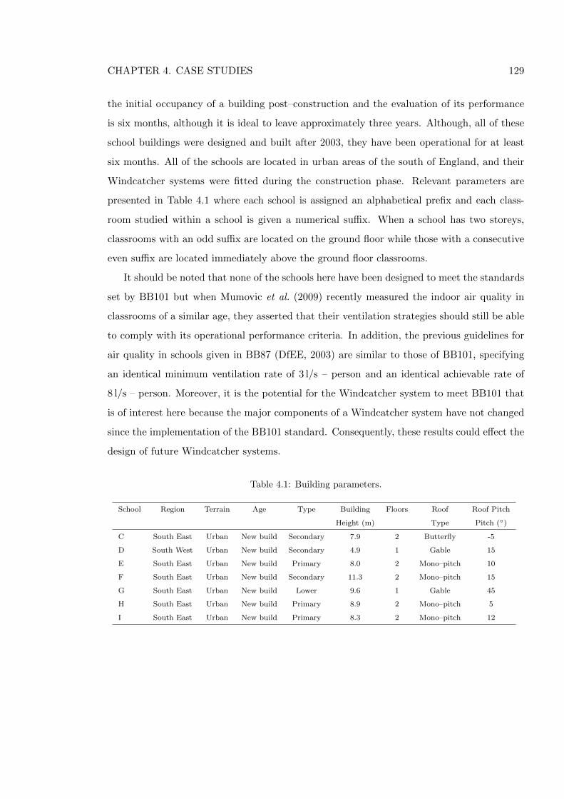
CHAPTER 4. CASE STUDIES 129
the initial occupancy of a building post–construction and the evaluation of its performance
is six months, although it is ideal to leave approximately three years. Although, all of these
school buildings were designed and built after 2003, they have been operational for at least
six months. All of the schools are located in urban areas of the south of England, and their
Windcatcher systems were fitted during the construction phase. Relevant parameters are
presented in Table 4.1 where each school is assigned an alphabetical prefix and each class-
room studied within a school is given a numerical suffix. When a school has two storeys,
classrooms with an odd suffix are located on the ground floor while those with a consecutive
even suffix are located immediately above the ground floor classrooms.
It should be noted that none of the schools here have been designed to meet the standards
set by BB101 but when Mumovic et al. (2009) recently measured the indoor air quality in
classrooms of a similar age, they asserted that their ventilation strategies should still be able
to comply with its operational performance criteria. In addition, the previous guidelines for
air quality in schools given in BB87 (DfEE, 2003) are similar to those of BB101, specifying
an identical minimum ventilation rate of 3 l/s – person and an identical achievable rate of
8 l/s – person. Moreover, it is the potential for the Windcatcher system to meet BB101 that
is of interest here because the major components of a Windcatcher system have not changed
since the implementation of the BB101 standard. Consequently, these results could effect the
design of future Windcatcher systems.
Table 4.1: Building parameters.
School Region Terrain Age Type Building Floors Roof Roof Pitch
Height (m) Type Pitch (◦)
C South East Urban New build Secondary 7.9 2 Butterfly -5
D South West Urban New build Secondary 4.9 1 Gable 15
E South East Urban New build Primary 8.0 2 Mono–pitch 10
F South East Urban New build Secondary 11.3 2 Mono–pitch 15
G South East Urban New build Lower 9.6 1 Gable 45
H South East Urban New build Primary 8.9 2 Mono–pitch 5
I South East Urban New build Primary 8.3 2 Mono–pitch 12
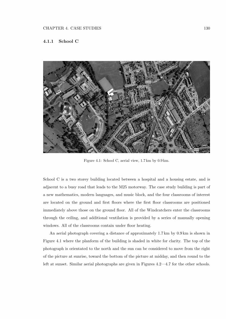
CHAPTER 4. CASE STUDIES 130
4.1.1 School C
Figure 4.1: School C, aerial view, 1.7 km by 0.9 km.
School C is a two storey building located between a hospital and a housing estate, and is
adjacent to a busy road that leads to the M25 motorway. The case study building is part of
a new mathematics, modern languages, and music block, and the four classrooms of interest
are located on the ground and first floors where the first floor classrooms are positioned
immediately above those on the ground floor. All of the Windcatchers enter the classrooms
through the ceiling, and additional ventilation is provided by a series of manually opening
windows. All of the classrooms contain under floor heating.
An aerial photograph covering a distance of approximately 1.7 km by 0.9 km is shown in
Figure 4.1 where the planform of the building is shaded in white for clarity. The top of the
photograph is orientated to the north and the sun can be considered to move from the right
of the picture at sunrise, toward the bottom of the picture at midday, and then round to the
left at sunset. Similar aerial photographs are given in Figures 4.2—4.7 for the other schools.
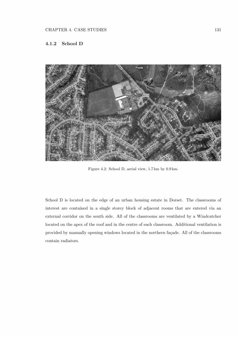
CHAPTER 4. CASE STUDIES 131
4.1.2 School D
Figure 4.2: School D, aerial view, 1.7 km by 0.9 km.
School D is located on the edge of an urban housing estate in Dorset. The classrooms of
interest are contained in a single storey block of adjacent rooms that are entered via an
external corridor on the south side. All of the classrooms are ventilated by a Windcatcher
located on the apex of the roof and in the centre of each classroom. Additional ventilation is
provided by manually opening windows located in the northern facade. All of the classrooms
contain radiators.
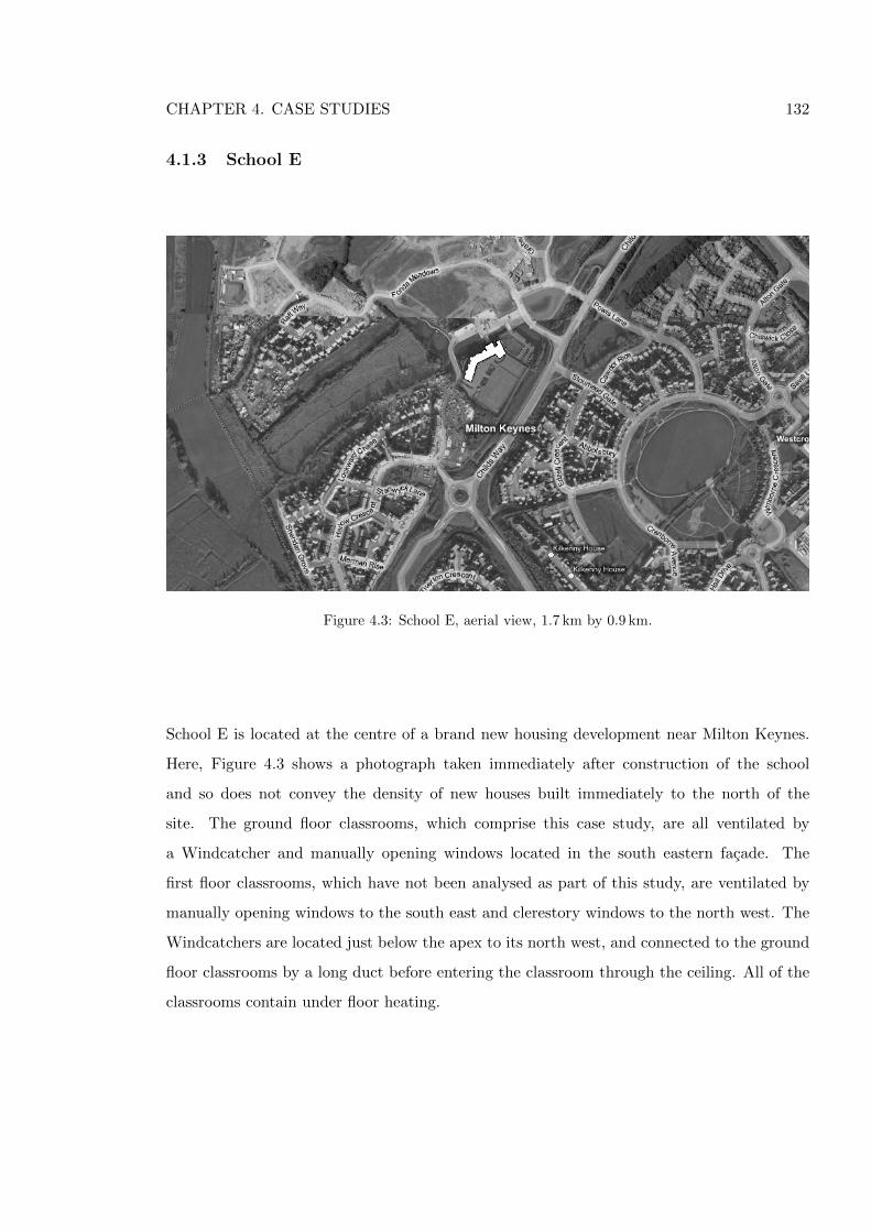
CHAPTER 4. CASE STUDIES 132
4.1.3 School E
Figure 4.3: School E, aerial view, 1.7 km by 0.9 km.
School E is located at the centre of a brand new housing development near Milton Keynes.
Here, Figure 4.3 shows a photograph taken immediately after construction of the school
and so does not convey the density of new houses built immediately to the north of the
site. The ground floor classrooms, which comprise this case study, are all ventilated by
a Windcatcher and manually opening windows located in the south eastern facade. The
first floor classrooms, which have not been analysed as part of this study, are ventilated by
manually opening windows to the south east and clerestory windows to the north west. The
Windcatchers are located just below the apex to its north west, and connected to the ground
floor classrooms by a long duct before entering the classroom through the ceiling. All of the
classrooms contain under floor heating.
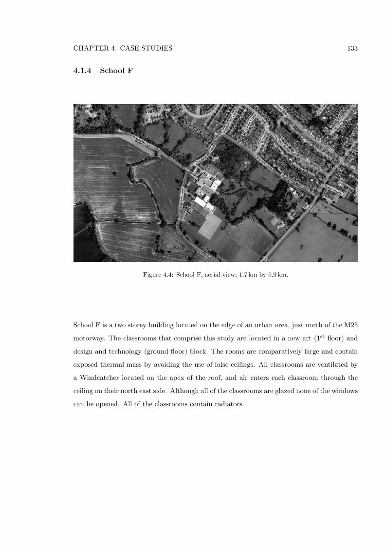
CHAPTER 4. CASE STUDIES 133
4.1.4 School F
Figure 4.4: School F, aerial view, 1.7 km by 0.9 km.
School F is a two storey building located on the edge of an urban area, just north of the M25
motorway. The classrooms that comprise this study are located in a new art (1st floor) and
design and technology (ground floor) block. The rooms are comparatively large and contain
exposed thermal mass by avoiding the use of false ceilings. All classrooms are ventilated by
a Windcatcher located on the apex of the roof, and air enters each classroom through the
ceiling on their north east side. Although all of the classrooms are glazed none of the windows
can be opened. All of the classrooms contain radiators.

CHAPTER 4. CASE STUDIES 134
4.1.5 School G
Figure 4.5: School G, aerial view, 0.6 km by 0.3 km.
School G is a single storey building located at the centre of a growing housing development.
Like school E, the development of the area has been rapid and so the photograph in Figure
4.5 does not convey the density of new houses built on all sides of the school. All of the
classrooms studied here are ventilated by a Windcatcher located on the apex of the roof
and ducted to each room through a false ceiling. Furthermore, each classroom contains sash
windows for additional ventilation that are housed the western facade and classroom G3 has
an additional window located in the southern facade. All of the classrooms contain radiators.
An aerial photograph is shown in Figure 4.5, but when compared to the photographs
of the other schools the scale has been increased to approximately 0.6 km by 0.3 km. This
is because available satellite photographs predate the construction of the school and could
mislead the reader at a larger scale. At the time of writing, on the vacant land located to
the east and south east of the school are buildings with heights that are greater than, or
equivalent to, the full height of the school.
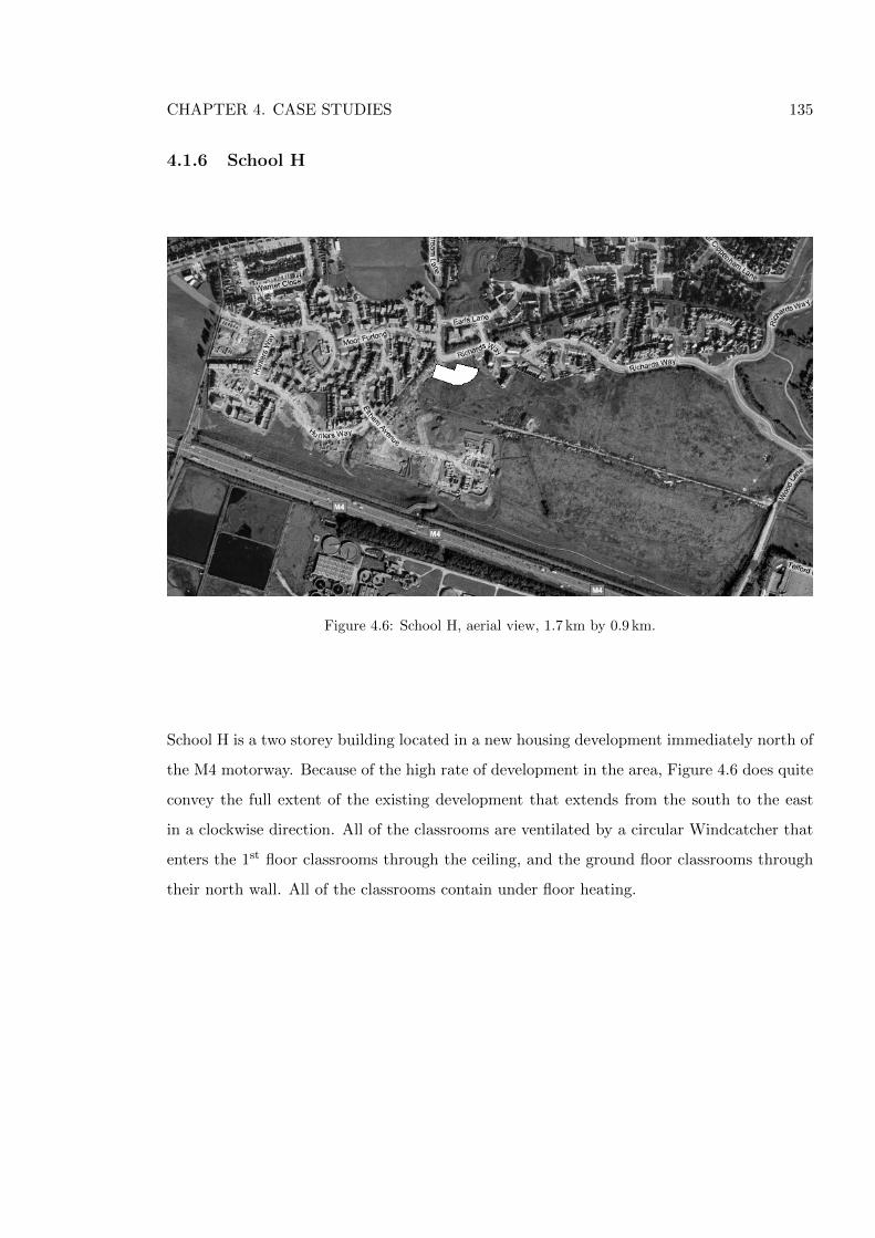
CHAPTER 4. CASE STUDIES 135
4.1.6 School H
Figure 4.6: School H, aerial view, 1.7 km by 0.9 km.
School H is a two storey building located in a new housing development immediately north of
the M4 motorway. Because of the high rate of development in the area, Figure 4.6 does quite
convey the full extent of the existing development that extends from the south to the east
in a clockwise direction. All of the classrooms are ventilated by a circular Windcatcher that
enters the 1st floor classrooms through the ceiling, and the ground floor classrooms through
their north wall. All of the classrooms contain under floor heating.
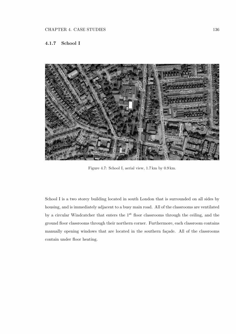
CHAPTER 4. CASE STUDIES 136
4.1.7 School I
Figure 4.7: School I, aerial view, 1.7 km by 0.9 km.
School I is a two storey building located in south London that is surrounded on all sides by
housing, and is immediately adjacent to a busy main road. All of the classrooms are ventilated
by a circular Windcatcher that enters the 1st floor classrooms through the ceiling, and the
ground floor classrooms through their northern corner. Furthermore, each classroom contains
manually opening windows that are located in the southern facade. All of the classrooms
contain under floor heating.
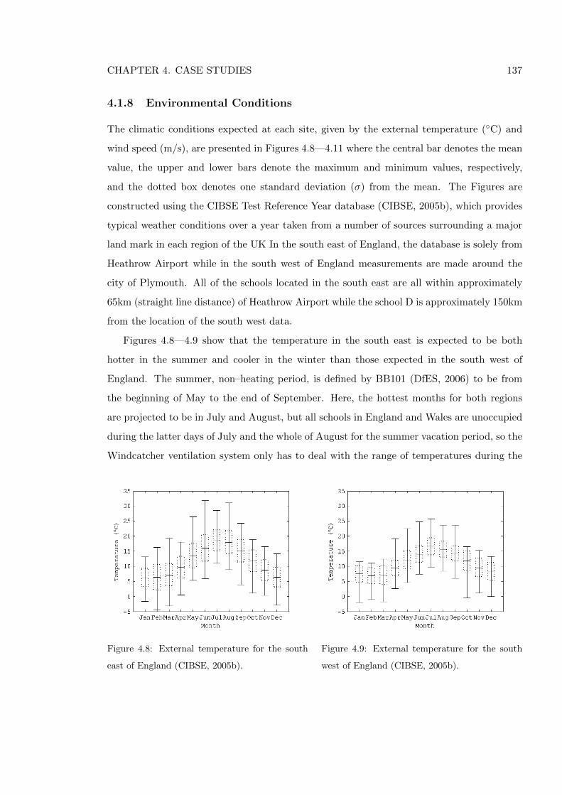
CHAPTER 4. CASE STUDIES 137
4.1.8 Environmental Conditions
The climatic conditions expected at each site, given by the external temperature (◦C) and
wind speed (m/s), are presented in Figures 4.8—4.11 where the central bar denotes the mean
value, the upper and lower bars denote the maximum and minimum values, respectively,
and the dotted box denotes one standard deviation (σ) from the mean. The Figures are
constructed using the CIBSE Test Reference Year database (CIBSE, 2005b), which provides
typical weather conditions over a year taken from a number of sources surrounding a major
land mark in each region of the UK In the south east of England, the database is solely from
Heathrow Airport while in the south west of England measurements are made around the
city of Plymouth. All of the schools located in the south east are all within approximately
65km (straight line distance) of Heathrow Airport while the school D is approximately 150km
from the location of the south west data.
Figures 4.8—4.9 show that the temperature in the south east is expected to be both
hotter in the summer and cooler in the winter than those expected in the south west of
England. The summer, non–heating period, is defined by BB101 (DfES, 2006) to be from
the beginning of May to the end of September. Here, the hottest months for both regions
are projected to be in July and August, but all schools in England and Wales are unoccupied
during the latter days of July and the whole of August for the summer vacation period, so the
Windcatcher ventilation system only has to deal with the range of temperatures during the
Figure 4.8: External temperature for the south
east of England (CIBSE, 2005b).
Figure 4.9: External temperature for the south
west of England (CIBSE, 2005b).
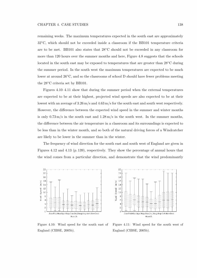
CHAPTER 4. CASE STUDIES 138
remaining weeks. The maximum temperatures expected in the south east are approximately
32◦C, which should not be exceeded inside a classroom if the BB101 temperature criteria
are to be met. BB101 also states that 28◦C should not be exceeded in any classroom for
more than 120 hours over the summer months and here, Figure 4.8 suggests that the schools
located in the south east may be exposed to temperatures that are greater than 28◦C during
the summer period. In the south west the maximum temperatures are expected to be much
lower at around 26◦C, and so the classrooms of school D should have fewer problems meeting
the 28◦C criteria set by BB101.
Figures 4.10–4.11 show that during the summer period when the external temperatures
are expected to be at their highest, projected wind speeds are also expected to be at their
lowest with an average of 3.26 m/s and 4.63 m/s for the south east and south west respectively.
However, the difference between the expected wind speed in the summer and winter months
is only 0.73 m/s in the south east and 1.28 m/s in the south west. In the summer months,
the difference between the air temperature in a classroom and its surroundings is expected to
be less than in the winter month, and so both of the natural driving forces of a Windcatcher
are likely to be lower in the summer than in the winter.
The frequency of wind direction for the south east and south west of England are given in
Figures 4.12 and 4.13 (p. 139), respectively. They show the percentage of annual hours that
the wind comes from a particular direction, and demonstrate that the wind predominantly
Figure 4.10: Wind speed for the south east of
England (CIBSE, 2005b).
Figure 4.11: Wind speed for the south west of
England (CIBSE, 2005b).
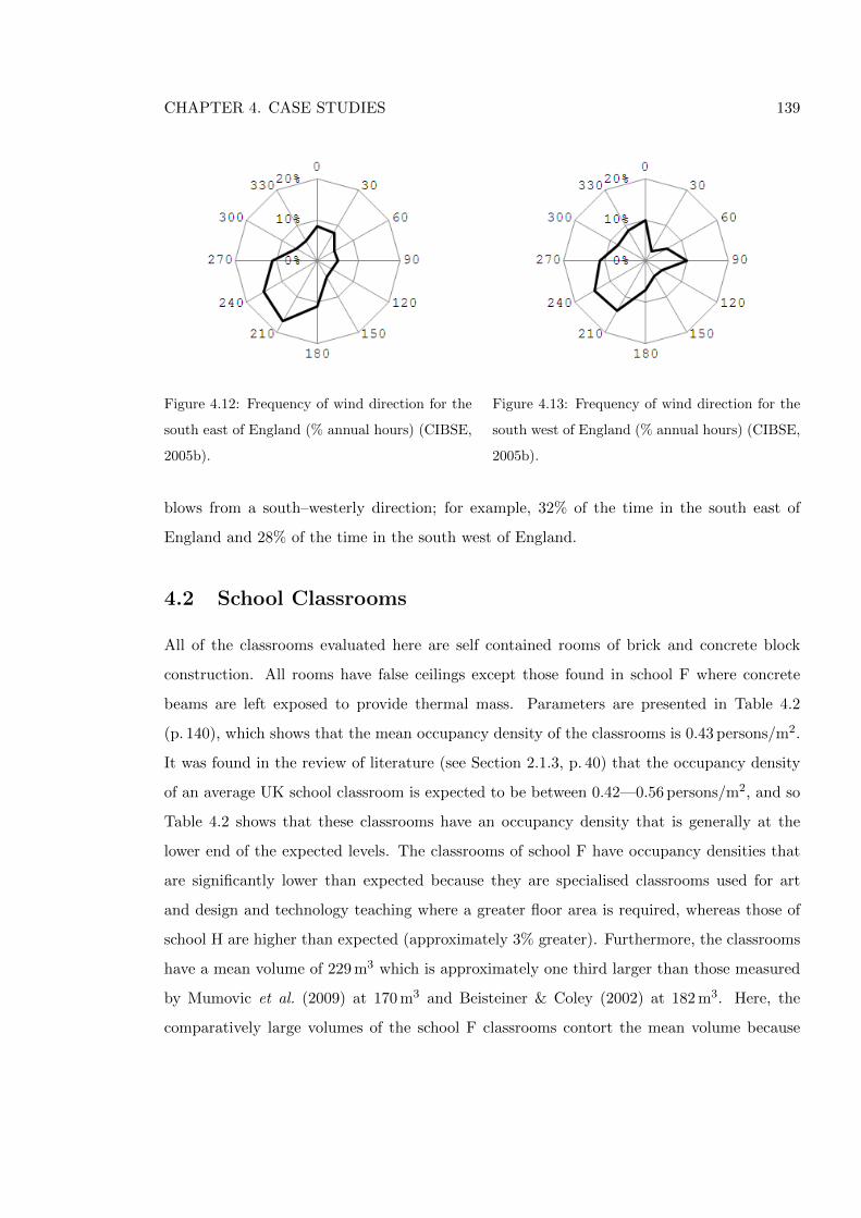
CHAPTER 4. CASE STUDIES 139
Figure 4.12: Frequency of wind direction for the
south east of England (% annual hours) (CIBSE,
2005b).
Figure 4.13: Frequency of wind direction for the
south west of England (% annual hours) (CIBSE,
2005b).
blows from a south–westerly direction; for example, 32% of the time in the south east of
England and 28% of the time in the south west of England.
4.2 School Classrooms
All of the classrooms evaluated here are self contained rooms of brick and concrete block
construction. All rooms have false ceilings except those found in school F where concrete
beams are left exposed to provide thermal mass. Parameters are presented in Table 4.2
(p. 140), which shows that the mean occupancy density of the classrooms is 0.43 persons/m2.
It was found in the review of literature (see Section 2.1.3, p. 40) that the occupancy density
of an average UK school classroom is expected to be between 0.42—0.56 persons/m2, and so
Table 4.2 shows that these classrooms have an occupancy density that is generally at the
lower end of the expected levels. The classrooms of school F have occupancy densities that
are significantly lower than expected because they are specialised classrooms used for art
and design and technology teaching where a greater floor area is required, whereas those of
school H are higher than expected (approximately 3% greater). Furthermore, the classrooms
have a mean volume of 229 m3 which is approximately one third larger than those measured
by Mumovic et al. (2009) at 170 m3 and Beisteiner & Coley (2002) at 182 m3. Here, the
comparatively large volumes of the school F classrooms contort the mean volume because
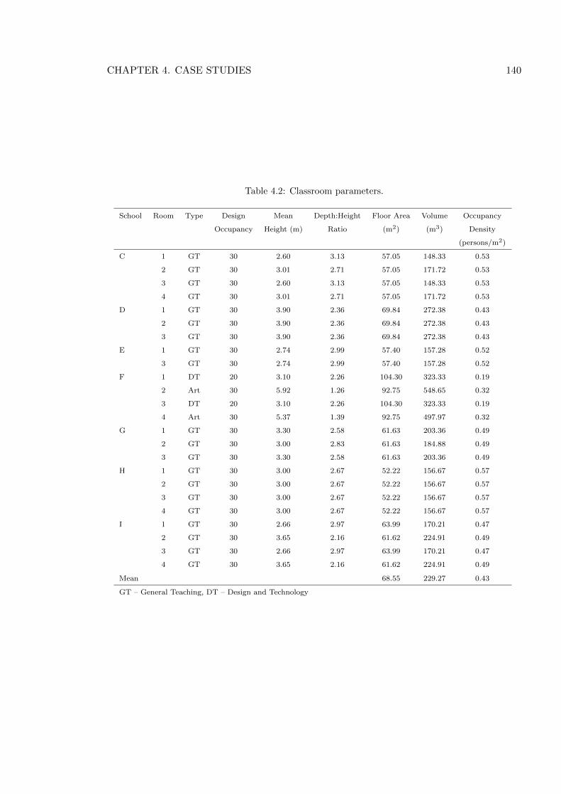
CHAPTER 4. CASE STUDIES 140
Table 4.2: Classroom parameters.
School Room Type Design Mean Depth:Height Floor Area Volume Occupancy
Occupancy Height (m) Ratio (m2) (m3) Density
(persons/m2)
C 1 GT 30 2.60 3.13 57.05 148.33 0.53
2 GT 30 3.01 2.71 57.05 171.72 0.53
3 GT 30 2.60 3.13 57.05 148.33 0.53
4 GT 30 3.01 2.71 57.05 171.72 0.53
D 1 GT 30 3.90 2.36 69.84 272.38 0.43
2 GT 30 3.90 2.36 69.84 272.38 0.43
3 GT 30 3.90 2.36 69.84 272.38 0.43
E 1 GT 30 2.74 2.99 57.40 157.28 0.52
3 GT 30 2.74 2.99 57.40 157.28 0.52
F 1 DT 20 3.10 2.26 104.30 323.33 0.19
2 Art 30 5.92 1.26 92.75 548.65 0.32
3 DT 20 3.10 2.26 104.30 323.33 0.19
4 Art 30 5.37 1.39 92.75 497.97 0.32
G 1 GT 30 3.30 2.58 61.63 203.36 0.49
2 GT 30 3.00 2.83 61.63 184.88 0.49
3 GT 30 3.30 2.58 61.63 203.36 0.49
H 1 GT 30 3.00 2.67 52.22 156.67 0.57
2 GT 30 3.00 2.67 52.22 156.67 0.57
3 GT 30 3.00 2.67 52.22 156.67 0.57
4 GT 30 3.00 2.67 52.22 156.67 0.57
I 1 GT 30 2.66 2.97 63.99 170.21 0.47
2 GT 30 3.65 2.16 61.62 224.91 0.49
3 GT 30 2.66 2.97 63.99 170.21 0.47
4 GT 30 3.65 2.16 61.62 224.91 0.49
Mean 68.55 229.27 0.43
GT – General Teaching, DT – Design and Technology
CHAPTER 4. CASE STUDIES 141
the mean volume of all classrooms except those of school F is 189 m3, which is much closer
to those measured by Beisteiner and Coley, and Mumovic et al.
All of the classrooms have a single wall of double glazing, which in classrooms F2, F4, I2,
and I4 is augmented by clerestory windows (here 77% and 45% of total glazing area at schools
F and I respectively). The area of the facade to the total glazing area is given by the glazing
ratio. Table 4.3 (p. 142) shows that classrooms with south facing classrooms generally have a
lower glazing ratio (see schools C and F) although the glazing ratio of school H is very high
and so its classrooms could experience over heating in the summer months. The windows
of school F are all sealed, but at the other schools, a number of windows can be opened
manually and so the estimated opening areas for these windows are presented in Table 4.3.
The openable area has been calculated using CIBSE guidelines (CIBSE, 2005a) that for a
top hung or bottom hung window takes into account the triangular area on each side of the
window, and so their area is given by
A5 = dO(wO + hO) (4.1)
where A5 is the estimated open area of a window, wO is the width of a window, hO is the
height of a window, and dO is the opening depth of a window.
The estimated openable area is found to range from 0.46 m2 to 3.88 m2 with a mean value
of 1.06 m2 per classroom which is 18% smaller than those reported by Mumovic et al. (2009).
Because openable windows are common in the majority of the classrooms and can be used
to contribute to the ventilation strategy, estimations of the ventilation rates through them
in coordination with a Windcatcher are made in Chapter 5, although it cannot be said if
the windows are open or not during the monitored periods because their position was not
recorded. Table 4.3 shows that some of the classrooms are south facing and although the
windows of the classrooms of school G are not shielded, the classrooms of schools E and I
(lower floor) are shielded by a balcony and those of school C, F, G, and I (upper floor) have
solar fins or slats to reduce solar heat gains.
All of the openable windows are positioned adjacent to each other in one or two rows.
In classrooms where two rows are found (schools E and I for example) the windows are
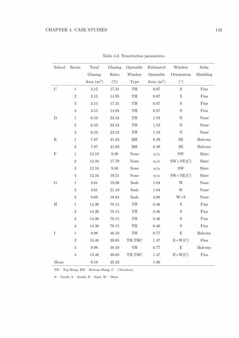
CHAPTER 4. CASE STUDIES 142
Table 4.3: Fenestration parameters.
School Room Total Glazing Openable Estimated Window Solar
Glazing Ratio Window Openable Orientation Shielding
Area (m2) (%) Type Area (m2) (◦)
C 1 3.15 17.31 TH 0.87 S Fins
2 3.15 14.95 TH 0.87 S Fins
3 3.15 17.31 TH 0.87 S Fins
4 3.15 14.95 TH 0.87 S Fins
D 1 6.53 23.24 TH 1.53 N None
2 6.53 23.24 TH 1.53 N None
3 6.53 23.24 TH 1.53 N None
E 1 7.87 41.03 BH 0.49 SE Balcony
3 7.87 41.03 BH 0.49 SE Balcony
F 1 12.10 9.30 None n/a SW Slats
2 12.34 17.70 None n/a SW+NE(C) Slats
3 12.10 9.30 None n/a SW Slats
4 12.34 19.51 None n/a SW+NE(C) Slats
G 1 4.61 19.26 Sash 1.84 W None
2 4.61 21.19 Sash 1.84 W None
3 9.69 18.64 Sash 3.88 W+S None
H 1 14.30 78.15 TH 0.46 S Fins
2 14.30 78.15 TH 0.46 S Fins
3 14.30 78.15 TH 0.46 S Fins
4 14.30 78.15 TH 0.46 S Fins
I 1 9.98 48.10 TH 0.77 E Balcony
2 13.40 39.05 TH,THC 1.47 E+W(C) Fins
3 9.98 48.10 TH 0.77 E Balcony
4 13.40 39.05 TH,THC 1.47 E+W(C) Fins
Mean 9.18 35.23 1.06
TH – Top Hung; BH – Bottom Hung; C – Clerestory.
N – North; S – South; E – East; W – West.
CHAPTER 4. CASE STUDIES 143
placed immediately on top of each other and so do not provide single–sided double–opening
ventilation (see Figure 2.2, p. 48) because their separation is less than 1.5 m (CIBSE, 2005a).
Therefore, in the absence of a Windcatcher they are only able to provide single–sided single–
opening ventilation (see Figure 2.1). Here, rule–of–thumb guidelines (CIBSE, 2005a) for the
effective penetration of air to the back of a room ventilated using single–sided single–opening
ventilation suggest that the depth to height ratio should be no greater than 2, but Table 4.2
shows that none of the classrooms meet this criteria. Nevertheless, all of the classrooms meet
the rule–of–thumb criteria (see CIBSE, 2005a) for successful cross–ventilation using windows
because their depth to hight ratio is less than 5, see Figure 2.3.
4.3 Ventilation Strategy and Control
Of the twenty four classrooms examined here, sixteen contain a square Windcatcher while
the remaining eight contain a circular Windcatcher, see Table 4.4 (p. 144). The ventilation
strategies employed in each classroom are presented in Figures 4.14—4.21 (from p. 145),
which show that the Windcatcher can be used to ventilate the classrooms autonomously
and in coordination with open windows to provide cross–ventilation in all of the classrooms,
except for those of school F, see Figure 4.17. In classrooms I2 and I4 the windows located in
the facade in coordination with the upper clerestory windows can provide cross–ventilation
without the Windcatcher, although this strategy relies upon the occupants to manually open
these windows, see Figure 4.20. When a classroom is located on the lowest floor of a multi–
storey building (see classrooms C1 and C3, Figure 4.14 for example), or where there is a
significant roof void between the false ceiling and the roof top (see school G, Figure 4.18),
the Windcatcher duct is generally much longer than those where there is a much smaller roof
void (see Table 4.4 for duct lengths). Figure 4.21 shows a cross–section view of the duct
transition in multi–storey buildings such as schools C, F, H, and I. The varying window area
and duct length provide an opportunity to develop the findings of Kolokotroni et al. (2002b)
who found that opening windows significantly increased the ventilation rates, and also noted
that ventilation rates measured on the ground floor were less than those measured on the
first floor, citing the length of the Windcatcher duct as a potential confounding factor.
All of the Windcatchers are diagonally divided for the length of the element, but not
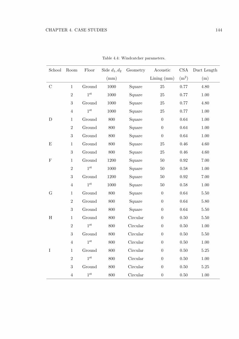
CHAPTER 4. CASE STUDIES 144
Table 4.4: Windcatcher parameters.
School Room Floor Side d1, d2 Geometry Acoustic CSA Duct Length
(mm) Lining (mm) (m2) (m)
C 1 Ground 1000 Square 25 0.77 4.80
2 1st 1000 Square 25 0.77 1.00
3 Ground 1000 Square 25 0.77 4.80
4 1st 1000 Square 25 0.77 1.00
D 1 Ground 800 Square 0 0.64 1.00
2 Ground 800 Square 0 0.64 1.00
3 Ground 800 Square 0 0.64 1.00
E 1 Ground 800 Square 25 0.46 4.60
3 Ground 800 Square 25 0.46 4.60
F 1 Ground 1200 Square 50 0.92 7.00
2 1st 1000 Square 50 0.58 1.00
3 Ground 1200 Square 50 0.92 7.00
4 1st 1000 Square 50 0.58 1.00
G 1 Ground 800 Square 0 0.64 5.50
2 Ground 800 Square 0 0.64 5.80
3 Ground 800 Square 0 0.64 5.50
H 1 Ground 800 Circular 0 0.50 5.50
2 1st 800 Circular 0 0.50 1.00
3 Ground 800 Circular 0 0.50 5.50
4 1st 800 Circular 0 0.50 1.00
I 1 Ground 800 Circular 0 0.50 5.25
2 1st 800 Circular 0 0.50 1.00
3 Ground 800 Circular 0 0.50 5.25
4 1st 800 Circular 0 0.50 1.00
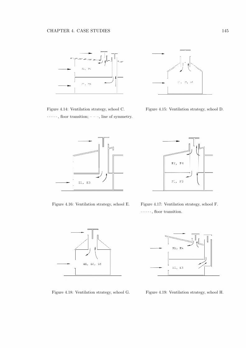
CHAPTER 4. CASE STUDIES 145
Figure 4.14: Ventilation strategy, school C.
· · · · · · , floor transition; – – –, line of symmetry.
Figure 4.15: Ventilation strategy, school D.
Figure 4.16: Ventilation strategy, school E. Figure 4.17: Ventilation strategy, school F.
· · · · · · , floor transition.
Figure 4.18: Ventilation strategy, school G. Figure 4.19: Ventilation strategy, school H.
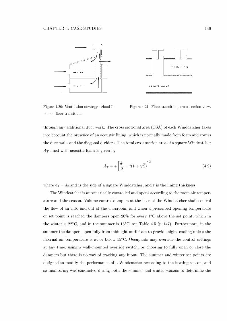
CHAPTER 4. CASE STUDIES 146
Figure 4.20: Ventilation strategy, school I.
· · · · · · , floor transition.
Figure 4.21: Floor transition, cross–section view.
through any additional duct work. The cross sectional area (CSA) of each Windcatcher takes
into account the presence of an acoustic lining, which is normally made from foam and covers
the duct walls and the diagonal dividers. The total cross section area of a square Windcatcher
AT lined with acoustic foam is given by
AT = 4
[d1
2− t(1 +
√2)
]2
(4.2)
where d1 = d2 and is the side of a square Windcatcher, and t is the lining thickness.
The Windcatcher is automatically controlled and opens according to the room air temper-
ature and the season. Volume control dampers at the base of the Windcatcher shaft control
the flow of air into and out of the classroom, and when a prescribed opening temperature
or set point is reached the dampers open 20% for every 1◦C above the set point, which in
the winter is 22◦C, and in the summer is 16◦C, see Table 4.5 (p. 147). Furthermore, in the
summer the dampers open fully from midnight until 6 am to provide night–cooling unless the
internal air temperature is at or below 15◦C. Occupants may override the control settings
at any time, using a wall–mounted override switch, by choosing to fully open or close the
dampers but there is no way of tracking any input. The summer and winter set points are
designed to modify the performance of a Windcatcher according to the heating season, and
so monitoring was conducted during both the summer and winter seasons to determine the
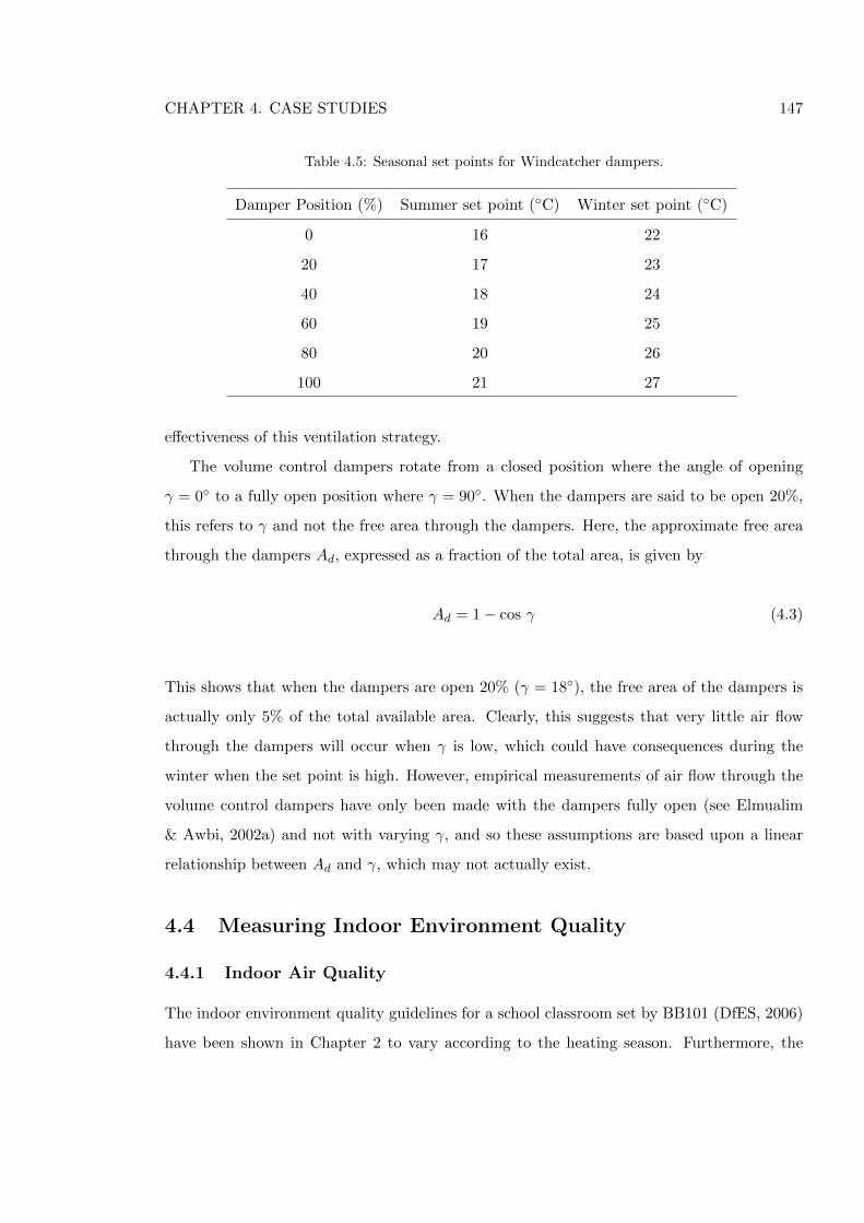
CHAPTER 4. CASE STUDIES 147
Table 4.5: Seasonal set points for Windcatcher dampers.
Damper Position (%) Summer set point (◦C) Winter set point (◦C)
0 16 22
20 17 23
40 18 24
60 19 25
80 20 26
100 21 27
effectiveness of this ventilation strategy.
The volume control dampers rotate from a closed position where the angle of opening
γ = 0◦ to a fully open position where γ = 90◦. When the dampers are said to be open 20%,
this refers to γ and not the free area through the dampers. Here, the approximate free area
through the dampers Ad, expressed as a fraction of the total area, is given by
Ad = 1− cos γ (4.3)
This shows that when the dampers are open 20% (γ = 18◦), the free area of the dampers is
actually only 5% of the total available area. Clearly, this suggests that very little air flow
through the dampers will occur when γ is low, which could have consequences during the
winter when the set point is high. However, empirical measurements of air flow through the
volume control dampers have only been made with the dampers fully open (see Elmualim
& Awbi, 2002a) and not with varying γ, and so these assumptions are based upon a linear
relationship between Ad and γ, which may not actually exist.
4.4 Measuring Indoor Environment Quality
4.4.1 Indoor Air Quality
The indoor environment quality guidelines for a school classroom set by BB101 (DfES, 2006)
have been shown in Chapter 2 to vary according to the heating season. Furthermore, the
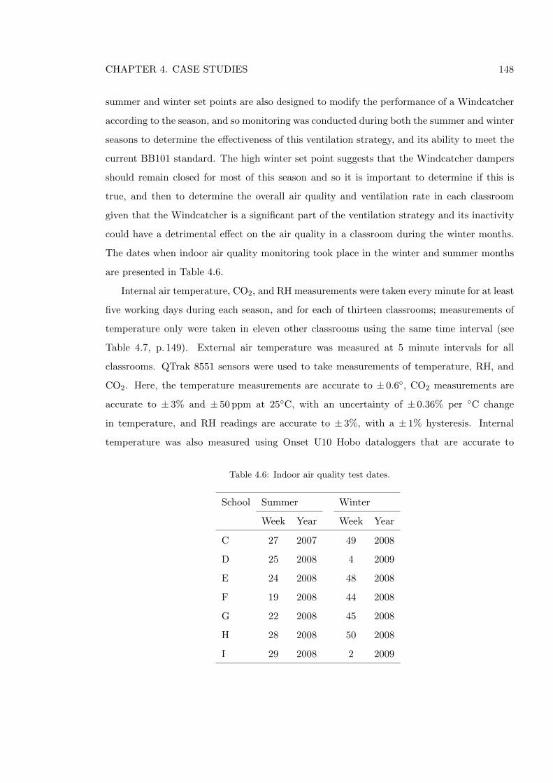
CHAPTER 4. CASE STUDIES 148
summer and winter set points are also designed to modify the performance of a Windcatcher
according to the season, and so monitoring was conducted during both the summer and winter
seasons to determine the effectiveness of this ventilation strategy, and its ability to meet the
current BB101 standard. The high winter set point suggests that the Windcatcher dampers
should remain closed for most of this season and so it is important to determine if this is
true, and then to determine the overall air quality and ventilation rate in each classroom
given that the Windcatcher is a significant part of the ventilation strategy and its inactivity
could have a detrimental effect on the air quality in a classroom during the winter months.
The dates when indoor air quality monitoring took place in the winter and summer months
are presented in Table 4.6.
Internal air temperature, CO2, and RH measurements were taken every minute for at least
five working days during each season, and for each of thirteen classrooms; measurements of
temperature only were taken in eleven other classrooms using the same time interval (see
Table 4.7, p. 149). External air temperature was measured at 5 minute intervals for all
classrooms. QTrak 8551 sensors were used to take measurements of temperature, RH, and
CO2. Here, the temperature measurements are accurate to ± 0.6◦, CO2 measurements are
accurate to ± 3% and ± 50 ppm at 25◦C, with an uncertainty of ± 0.36% per ◦C change
in temperature, and RH readings are accurate to ± 3%, with a ± 1% hysteresis. Internal
temperature was also measured using Onset U10 Hobo dataloggers that are accurate to
Table 4.6: Indoor air quality test dates.
School Summer Winter
Week Year Week Year
C 27 2007 49 2008
D 25 2008 4 2009
E 24 2008 48 2008
F 19 2008 44 2008
G 22 2008 45 2008
H 28 2008 50 2008
I 29 2008 2 2009
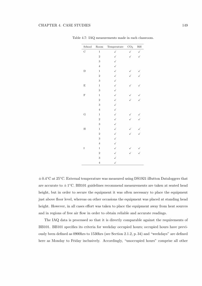
CHAPTER 4. CASE STUDIES 149
Table 4.7: IAQ measurements made in each classroom.
School Room Temperature CO2 RH
C 1 X X X
2 X X X
3 X
4 X
D 1 X X X
2 X X X
3 X
E 1 X X X
3 X
F 1 X X X
2 X X X
3 X
4 X
G 1 X X X
2 X X X
3 X
H 1 X X X
2 X X X
3 X
4 X
I 1 X X X
2 X X X
3 X
4 X
± 0.4◦C at 25◦C. External temperature was measured using DS1921 iButton Dataloggers that
are accurate to ± 1◦C. BB101 guidelines recommend measurements are taken at seated head
height, but in order to secure the equipment it was often necessary to place the equipment
just above floor level, whereas on other occasions the equipment was placed at standing head
height. However, in all cases effort was taken to place the equipment away from heat sources
and in regions of free air flow in order to obtain reliable and accurate readings.
The IAQ data is processed so that it is directly comparable against the requirements of
BB101. BB101 specifies its criteria for weekday occupied hours; occupied hours have previ-
ously been defined as 0900hrs to 1530hrs (see Section 2.1.2, p. 34) and “weekdays” are defined
here as Monday to Friday inclusively. Accordingly, “unoccupied hours” comprise all other
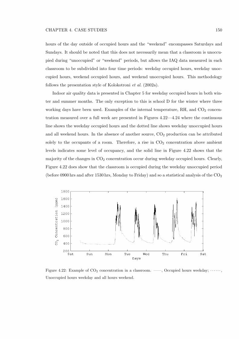
CHAPTER 4. CASE STUDIES 150
hours of the day outside of occupied hours and the “weekend” encompasses Saturdays and
Sundays. It should be noted that this does not necessarily mean that a classroom is unoccu-
pied during “unoccupied” or “weekend” periods, but allows the IAQ data measured in each
classroom to be subdivided into four time periods: weekday occupied hours, weekday unoc-
cupied hours, weekend occupied hours, and weekend unoccupied hours. This methodology
follows the presentation style of Kolokotroni et al. (2002a).
Indoor air quality data is presented in Chapter 5 for weekday occupied hours in both win-
ter and summer months. The only exception to this is school D for the winter where three
working days have been used. Examples of the internal temperature, RH, and CO2 concen-
tration measured over a full week are presented in Figures 4.22—4.24 where the continuous
line shows the weekday occupied hours and the dotted line shows weekday unoccupied hours
and all weekend hours. In the absence of another source, CO2 production can be attributed
solely to the occupants of a room. Therefore, a rise in CO2 concentration above ambient
levels indicates some level of occupancy, and the solid line in Figure 4.22 shows that the
majority of the changes in CO2 concentration occur during weekday occupied hours. Clearly,
Figure 4.22 does show that the classroom is occupied during the weekday unoccupied period
(before 0900 hrs and after 1530 hrs, Monday to Friday) and so a statistical analysis of the CO2
Figure 4.22: Example of CO2 concentration in a classroom. ——, Occupied hours weekday; · · · · · · ,
Unoccupied hours weekday and all hours weekend.
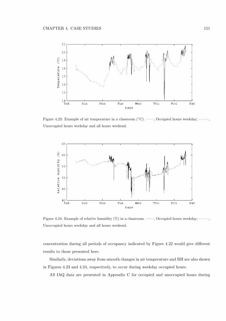
CHAPTER 4. CASE STUDIES 151
Figure 4.23: Example of air temperature in a classroom (◦C). ——, Occupied hours weekday; · · · · · · ,
Unoccupied hours weekday and all hours weekend.
Figure 4.24: Example of relative humidity (%) in a classroom. ——, Occupied hours weekday; · · · · · · ,
Unoccupied hours weekday and all hours weekend.
concentration during all periods of occupancy indicated by Figure 4.22 would give different
results to those presented here.
Similarly, deviations away from smooth changes in air temperature and RH are also shown
in Figures 4.23 and 4.24, respectively, to occur during weekday occupied hours.
All IAQ data are presented in Appendix C for occupied and unoccupied hours during
CHAPTER 4. CASE STUDIES 152
the working week and at the weekend. All calculations were made using MATLAB and have
been corroborated using Microsoft Excel spreadsheets.
4.4.2 Ventilation Rate
The total ventilation rate in each classroom was measured using the tracer gas decay method,
which is well documented by Etheridge & Sandberg (1996) and Liddament (1996). Here, a
small amount of sulphur hexafluoride (SF6) was chosen as a tracer gas and injected into a
classroom where it was thoroughly mixed using fans to establish a uniform concentration.
Then, its exponential decay was monitored every 45 seconds using an Innova 1312 dual
gas analyser that has a repeatability of reading of 1%. Measurements were taken from the
centre of the room for periods of no less than 20 minutes in accordance with the guidelines
of Liddament. Mixing fans were not used during measurement periods because Liddament
(1996) suggests that they create artificial flow paths so that measured conditions do not
represent occupied conditions; this methodology is also followed by Kirk (2004a) and Pegg
(2008). None of the classrooms measured here were interconnected except for those in School
F. Here, classrooms F1 and F3, and classrooms F2 and F4 are interconnected but the doors
were kept closed to replicated occupied conditions. Adjacent classrooms and corridoors were
not seeded with the tracer gas, and so the measurement of ventilation rate does not distinguish
between air supplied from outside, through a Windcatcher for example, or from adjacent
classrooms.
The concentration of a gas at any instant in time is given by the following continuity
equation (Coley & Beisteiner, 2002)
V∂C(t)
∂t= G+ QT [CE − C(t)] (4.4)
where V is the volume of the room (m3), QT is the total air flow rate (m3/s) into and out of
the room, C(t) is the concentration (ppm) of the gas at any moment in time t, C(0) is the
initial concentration of the gas (when time t = 0), CE is the external concentration of the
gas. Now, solving Equation (4.4) by integrating between t = 0 and a time t gives
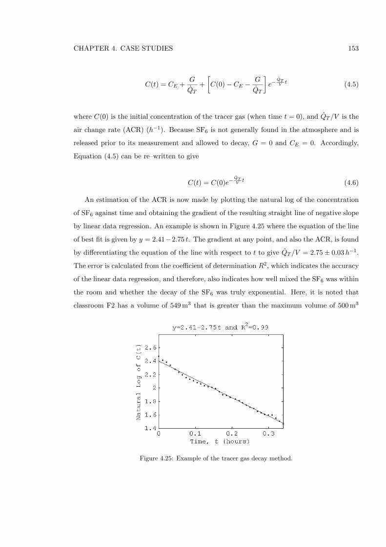
CHAPTER 4. CASE STUDIES 153
C(t) = CE +G
QT
+
[C(0)− CE −
G
QT
]e−
QTV
t (4.5)
where C(0) is the initial concentration of the tracer gas (when time t = 0), and QT /V is the
air change rate (ACR) (h−1). Because SF6 is not generally found in the atmosphere and is
released prior to its measurement and allowed to decay, G = 0 and CE = 0. Accordingly,
Equation (4.5) can be re–written to give
C(t) = C(0)e−QTV
t (4.6)
An estimation of the ACR is now made by plotting the natural log of the concentration
of SF6 against time and obtaining the gradient of the resulting straight line of negative slope
by linear data regression. An example is shown in Figure 4.25 where the equation of the line
of best fit is given by y = 2.41−2.75 t. The gradient at any point, and also the ACR, is found
by differentiating the equation of the line with respect to t to give QT /V = 2.75± 0.03h−1.
The error is calculated from the coefficient of determination R2, which indicates the accuracy
of the linear data regression, and therefore, also indicates how well mixed the SF6 was within
the room and whether the decay of the SF6 was truly exponential. Here, it is noted that
classroom F2 has a volume of 549 m3 that is greater than the maximum volume of 500 m3
Figure 4.25: Example of the tracer gas decay method.
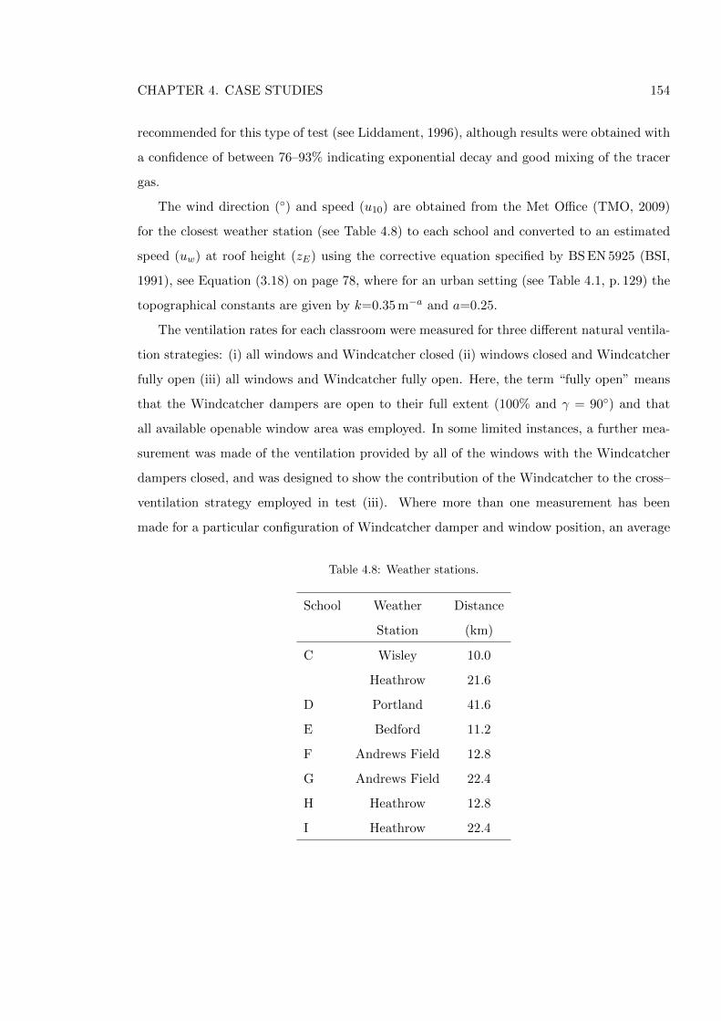
CHAPTER 4. CASE STUDIES 154
recommended for this type of test (see Liddament, 1996), although results were obtained with
a confidence of between 76–93% indicating exponential decay and good mixing of the tracer
gas.
The wind direction (◦) and speed (u10) are obtained from the Met Office (TMO, 2009)
for the closest weather station (see Table 4.8) to each school and converted to an estimated
speed (uw) at roof height (zE) using the corrective equation specified by BS EN 5925 (BSI,
1991), see Equation (3.18) on page 78, where for an urban setting (see Table 4.1, p. 129) the
topographical constants are given by k=0.35 m−a and a=0.25.
The ventilation rates for each classroom were measured for three different natural ventila-
tion strategies: (i) all windows and Windcatcher closed (ii) windows closed and Windcatcher
fully open (iii) all windows and Windcatcher fully open. Here, the term “fully open” means
that the Windcatcher dampers are open to their full extent (100% and γ = 90◦) and that
all available openable window area was employed. In some limited instances, a further mea-
surement was made of the ventilation provided by all of the windows with the Windcatcher
dampers closed, and was designed to show the contribution of the Windcatcher to the cross–
ventilation strategy employed in test (iii). Where more than one measurement has been
made for a particular configuration of Windcatcher damper and window position, an average
Table 4.8: Weather stations.
School Weather Distance
Station (km)
C Wisley 10.0
Heathrow 21.6
D Portland 41.6
E Bedford 11.2
F Andrews Field 12.8
G Andrews Field 22.4
H Heathrow 12.8
I Heathrow 22.4
CHAPTER 4. CASE STUDIES 155
value is used. Furthermore, where there are several variations of the same configuration, for
example at schools G and I where windows are located on two facades, estimations of the
ventilation rate using the maximum openable window area are used in Table 5.2, (p. 168).
Estimates of background ventilation rates (with Windcatcher and windows closed) were not
made in classrooms C3 and C4 due to time constraints, whereas in classrooms D2 and D3
the override controllers were damaged. In classroom G2, despite several attempts, a satis-
factory estimate could not be made and so the classroom is considered to be tightly sealed
with negligible background ventilation. It was also not possible to make estimations with the
Windcatcher open and windows closed in classrooms I1 and I3 because the damper override
was temporarily locked by the BMS in response to a boiler failure.
4.4.3 Noise
Acoustic measurements of the equivalent sound pressure level over 30 minutes (LAeq,30m) were
made using a Cirrus CR262 Sound Level Meter that is accurate to ± 0.5 dB and DeafDefier
software. The meter was placed in the centre of the room and measurements made with
all windows closed and the Windcatcher dampers either open or closed. External LAeq,30m
was measured adjacent to the facade of the classroom. Here, it is noted that the upper
limits specified by BB93 (DfES, 2003) are for an unoccupied and unfurnished classroom, but
it was not possible to test the classrooms under these circumstances because, although the
classrooms were unoccupied, they were not free from furnishings.
4.5 Summary
In Chapter 2 the indoor environment quality in a classroom ventilated by a Windcatcher
was found to be a function of ventilation and noise, and the control of them. Furthermore,
the literature also shows that there is a lack of data for a Windcatcher when measured in–
situ and that a quantitative analysis of their performance would establish their performance
when compared against the UK government standards for ventilation, indoor air quality, and
noise. Accordingly, this Chapter has introduced seven case study buildings that have been
chosen to demonstrate Windcatcher performance in–situ in a variety of environments and
for a number of configurations. Because over 70% of Windcatcher systems are installed into
CHAPTER 4. CASE STUDIES 156
school buildings, all of the case study buildings are schools. Here, twenty four classrooms have
been selected and their parameters have been compared against those found in the literature.
A methodology for the measurement of IAQ, ventilation, and noise has been discussed, so
that the findings may be compared against the current standards set by BB101 and BB93,
and an indication of Windcatcher performance can be determined. Finally, the case studies
also have a secondary function; the data collected from them will contribute to the limited
number of published reviews of air quality and ventilation rates in UK school classrooms.
The results are presented in Chapters 5 and 6.

CHAPTER 5. RESULTS: IEQ IN CASE STUDY CLASSROOMS 157
Chapter 5
Results: IEQ in Case Study
Classrooms
This chapter presents the measurements of key indoor air quality parameters, ventilation
rates, and background noise for each classroom of the seven case study schools. Measurements
of air temperature for twenty four classrooms, and CO2 and RH for thirteen classrooms are
presented in Section 5.1, and sound pressure levels are presented for twenty three classrooms in
Section 5.3. The data is plotted so that it is easily compared with the requirements of BB101
(DfES, 2006), BB93 (DfES, 2003), or other relevant standards, and equivalent measurements
for UK school classrooms available in the literature. Because the measurements of IAQ
are largely determined by the ventilation rate delivered to each classroom, which in turn is
an important indicator of the overall success of the ventilation strategy in each classroom,
estimated ventilation rates for three key configurations are presented in Section 5.2.
5.1 Indoor Air Quality
The results presented in this section have been collated using the methodology described in
Section 4.4 (p. 147).
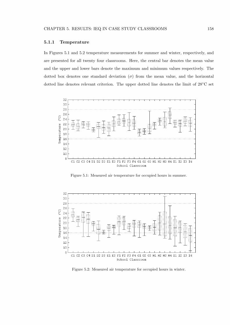
CHAPTER 5. RESULTS: IEQ IN CASE STUDY CLASSROOMS 158
5.1.1 Temperature
In Figures 5.1 and 5.2 temperature measurements for summer and winter, respectively, and
are presented for all twenty four classrooms. Here, the central bar denotes the mean value
and the upper and lower bars denote the maximum and minimum values respectively. The
dotted box denotes one standard deviation (σ) from the mean value, and the horizontal
dotted line denotes relevant criterion. The upper dotted line denotes the limit of 28◦C set
Figure 5.1: Measured air temperature for occupied hours in summer.
Figure 5.2: Measured air temperature for occupied hours in winter.
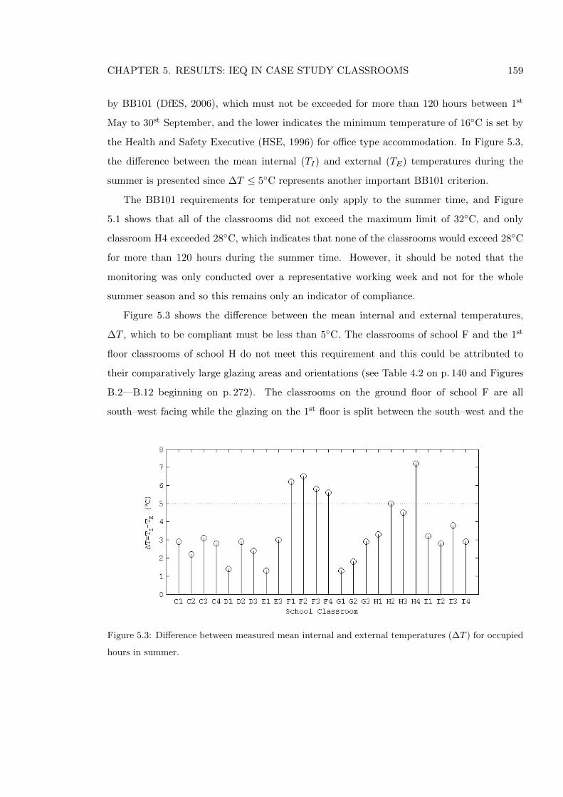
CHAPTER 5. RESULTS: IEQ IN CASE STUDY CLASSROOMS 159
by BB101 (DfES, 2006), which must not be exceeded for more than 120 hours between 1st
May to 30st September, and the lower indicates the minimum temperature of 16◦C is set by
the Health and Safety Executive (HSE, 1996) for office type accommodation. In Figure 5.3,
the difference between the mean internal (TI) and external (TE) temperatures during the
summer is presented since ∆T ≤ 5◦C represents another important BB101 criterion.
The BB101 requirements for temperature only apply to the summer time, and Figure
5.1 shows that all of the classrooms did not exceed the maximum limit of 32◦C, and only
classroom H4 exceeded 28◦C, which indicates that none of the classrooms would exceed 28◦C
for more than 120 hours during the summer time. However, it should be noted that the
monitoring was only conducted over a representative working week and not for the whole
summer season and so this remains only an indicator of compliance.
Figure 5.3 shows the difference between the mean internal and external temperatures,
∆T , which to be compliant must be less than 5◦C. The classrooms of school F and the 1st
floor classrooms of school H do not meet this requirement and this could be attributed to
their comparatively large glazing areas and orientations (see Table 4.2 on p. 140 and Figures
B.2—B.12 beginning on p. 272). The classrooms on the ground floor of school F are all
south–west facing while the glazing on the 1st floor is split between the south–west and the
Figure 5.3: Difference between measured mean internal and external temperatures (∆T ) for occupied
hours in summer.
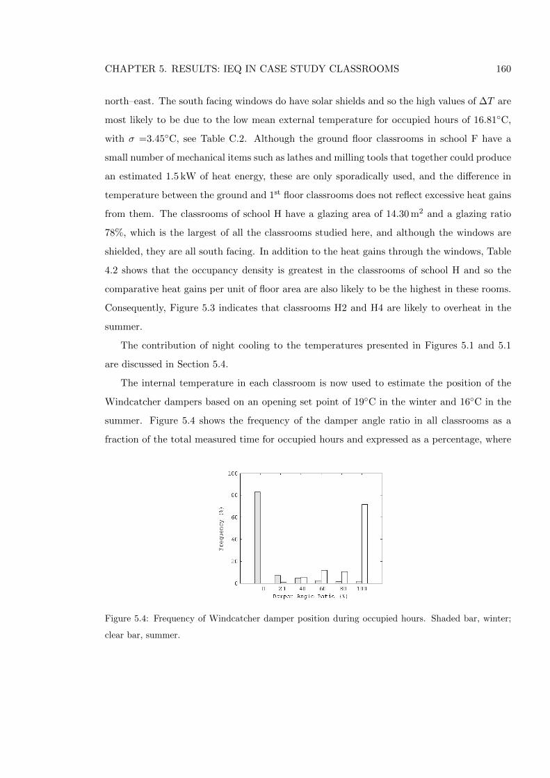
CHAPTER 5. RESULTS: IEQ IN CASE STUDY CLASSROOMS 160
north–east. The south facing windows do have solar shields and so the high values of ∆T are
most likely to be due to the low mean external temperature for occupied hours of 16.81◦C,
with σ =3.45◦C, see Table C.2. Although the ground floor classrooms in school F have a
small number of mechanical items such as lathes and milling tools that together could produce
an estimated 1.5 kW of heat energy, these are only sporadically used, and the difference in
temperature between the ground and 1st floor classrooms does not reflect excessive heat gains
from them. The classrooms of school H have a glazing area of 14.30 m2 and a glazing ratio
78%, which is the largest of all the classrooms studied here, and although the windows are
shielded, they are all south facing. In addition to the heat gains through the windows, Table
4.2 shows that the occupancy density is greatest in the classrooms of school H and so the
comparative heat gains per unit of floor area are also likely to be the highest in these rooms.
Consequently, Figure 5.3 indicates that classrooms H2 and H4 are likely to overheat in the
summer.
The contribution of night cooling to the temperatures presented in Figures 5.1 and 5.1
are discussed in Section 5.4.
The internal temperature in each classroom is now used to estimate the position of the
Windcatcher dampers based on an opening set point of 19◦C in the winter and 16◦C in the
summer. Figure 5.4 shows the frequency of the damper angle ratio in all classrooms as a
fraction of the total measured time for occupied hours and expressed as a percentage, where
Figure 5.4: Frequency of Windcatcher damper position during occupied hours. Shaded bar, winter;
clear bar, summer.
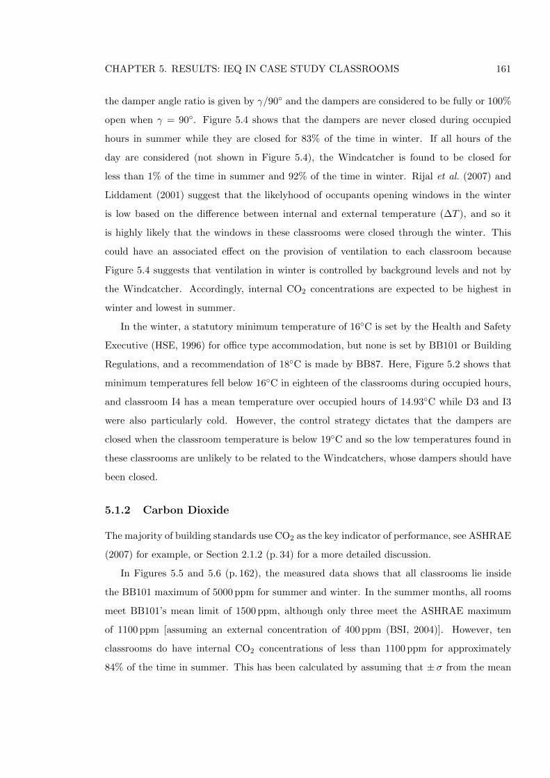
CHAPTER 5. RESULTS: IEQ IN CASE STUDY CLASSROOMS 161
the damper angle ratio is given by γ/90◦ and the dampers are considered to be fully or 100%
open when γ = 90◦. Figure 5.4 shows that the dampers are never closed during occupied
hours in summer while they are closed for 83% of the time in winter. If all hours of the
day are considered (not shown in Figure 5.4), the Windcatcher is found to be closed for
less than 1% of the time in summer and 92% of the time in winter. Rijal et al. (2007) and
Liddament (2001) suggest that the likelyhood of occupants opening windows in the winter
is low based on the difference between internal and external temperature (∆T ), and so it
is highly likely that the windows in these classrooms were closed through the winter. This
could have an associated effect on the provision of ventilation to each classroom because
Figure 5.4 suggests that ventilation in winter is controlled by background levels and not by
the Windcatcher. Accordingly, internal CO2 concentrations are expected to be highest in
winter and lowest in summer.
In the winter, a statutory minimum temperature of 16◦C is set by the Health and Safety
Executive (HSE, 1996) for office type accommodation, but none is set by BB101 or Building
Regulations, and a recommendation of 18◦C is made by BB87. Here, Figure 5.2 shows that
minimum temperatures fell below 16◦C in eighteen of the classrooms during occupied hours,
and classroom I4 has a mean temperature over occupied hours of 14.93◦C while D3 and I3
were also particularly cold. However, the control strategy dictates that the dampers are
closed when the classroom temperature is below 19◦C and so the low temperatures found in
these classrooms are unlikely to be related to the Windcatchers, whose dampers should have
been closed.
5.1.2 Carbon Dioxide
The majority of building standards use CO2 as the key indicator of performance, see ASHRAE
(2007) for example, or Section 2.1.2 (p. 34) for a more detailed discussion.
In Figures 5.5 and 5.6 (p. 162), the measured data shows that all classrooms lie inside
the BB101 maximum of 5000 ppm for summer and winter. In the summer months, all rooms
meet BB101’s mean limit of 1500 ppm, although only three meet the ASHRAE maximum
of 1100 ppm [assuming an external concentration of 400 ppm (BSI, 2004)]. However, ten
classrooms do have internal CO2 concentrations of less than 1100 ppm for approximately
84% of the time in summer. This has been calculated by assuming that ±σ from the mean
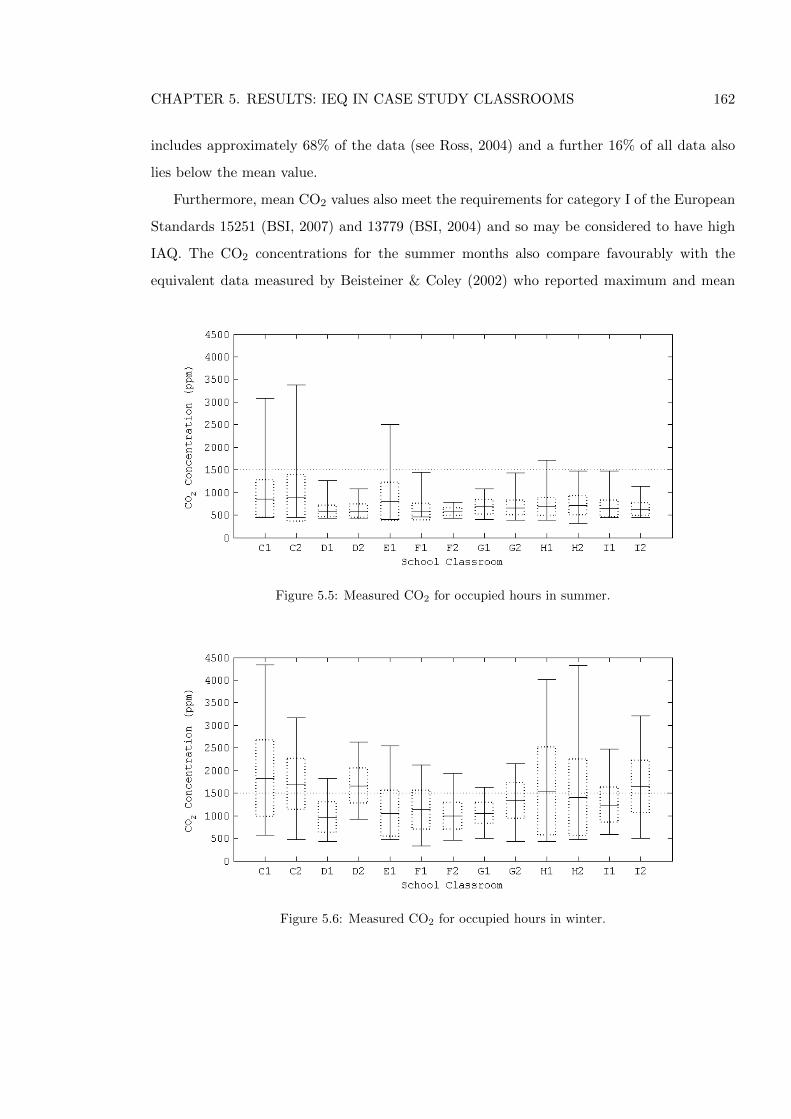
CHAPTER 5. RESULTS: IEQ IN CASE STUDY CLASSROOMS 162
includes approximately 68% of the data (see Ross, 2004) and a further 16% of all data also
lies below the mean value.
Furthermore, mean CO2 values also meet the requirements for category I of the European
Standards 15251 (BSI, 2007) and 13779 (BSI, 2004) and so may be considered to have high
IAQ. The CO2 concentrations for the summer months also compare favourably with the
equivalent data measured by Beisteiner & Coley (2002) who reported maximum and mean
Figure 5.5: Measured CO2 for occupied hours in summer.
Figure 5.6: Measured CO2 for occupied hours in winter.
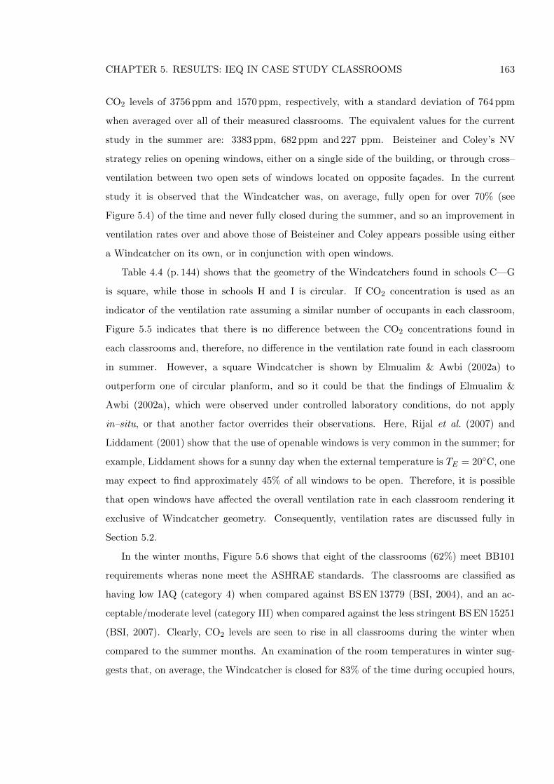
CHAPTER 5. RESULTS: IEQ IN CASE STUDY CLASSROOMS 163
CO2 levels of 3756 ppm and 1570 ppm, respectively, with a standard deviation of 764 ppm
when averaged over all of their measured classrooms. The equivalent values for the current
study in the summer are: 3383 ppm, 682 ppm and 227 ppm. Beisteiner and Coley’s NV
strategy relies on opening windows, either on a single side of the building, or through cross–
ventilation between two open sets of windows located on opposite facades. In the current
study it is observed that the Windcatcher was, on average, fully open for over 70% (see
Figure 5.4) of the time and never fully closed during the summer, and so an improvement in
ventilation rates over and above those of Beisteiner and Coley appears possible using either
a Windcatcher on its own, or in conjunction with open windows.
Table 4.4 (p. 144) shows that the geometry of the Windcatchers found in schools C—G
is square, while those in schools H and I is circular. If CO2 concentration is used as an
indicator of the ventilation rate assuming a similar number of occupants in each classroom,
Figure 5.5 indicates that there is no difference between the CO2 concentrations found in
each classrooms and, therefore, no difference in the ventilation rate found in each classroom
in summer. However, a square Windcatcher is shown by Elmualim & Awbi (2002a) to
outperform one of circular planform, and so it could be that the findings of Elmualim &
Awbi (2002a), which were observed under controlled laboratory conditions, do not apply
in–situ, or that another factor overrides their observations. Here, Rijal et al. (2007) and
Liddament (2001) show that the use of openable windows is very common in the summer; for
example, Liddament shows for a sunny day when the external temperature is TE = 20◦C, one
may expect to find approximately 45% of all windows to be open. Therefore, it is possible
that open windows have affected the overall ventilation rate in each classroom rendering it
exclusive of Windcatcher geometry. Consequently, ventilation rates are discussed fully in
Section 5.2.
In the winter months, Figure 5.6 shows that eight of the classrooms (62%) meet BB101
requirements wheras none meet the ASHRAE standards. The classrooms are classified as
having low IAQ (category 4) when compared against BS EN 13779 (BSI, 2004), and an ac-
ceptable/moderate level (category III) when compared against the less stringent BS EN 15251
(BSI, 2007). Clearly, CO2 levels are seen to rise in all classrooms during the winter when
compared to the summer months. An examination of the room temperatures in winter sug-
gests that, on average, the Windcatcher is closed for 83% of the time during occupied hours,
CHAPTER 5. RESULTS: IEQ IN CASE STUDY CLASSROOMS 164
and it is highly likely that the windows remained closed throughout the testing period. Ac-
cordingly, in winter the CO2 levels are largely controlled by background ventilation and this
is the likely cause of the rise in CO2 levels seen in the winter months. In Table 5.1 CO2
levels for winter are compared with those measured by Mumovic et al. (2009) and Coley &
Beisteiner (2002), and are shown to be higher than the MV classrooms and generally com-
parable to the NV classrooms reported by Mumovic et al., but much lower than Coley and
Beisteiner. Here, it seems likely that for each study the ventilation rates are dominated by
background ventilation during the winter months, and so it is difficult to be certain why
improvements have been found in the current study. Differences in ventilation rates may
simply be caused by differences in the fabric of each building, although it is noticeable that
in the two rooms studied by Mumovic et al. (2009) that adopt stack driven ventilation, CO2
levels are similar to those found in the current study. What is clear, however, is that if one
relies simply on opening windows to control CO2 levels during the winter months then there
is a significant risk of failure to meet BB101 requirements, see Coley & Beisteiner (2002).
Therefore, a Windcatcher offers an alternative strategy with the potential of lowering CO2
levels in winter by partially opening the Windcatcher dampers, although it would appear
necessary to set the Windcatcher controls to open at a given CO2 level rather than at a
pre–determined temperature, which was the strategy employed by the classrooms measured
here.
Santamouris et al. (2008) extensively reviewed the literature collating measurements of
ventilation rate and internal CO2 concentration during occupied hours from 1187 classrooms,
of which 287 are NV and 900 are MV, to form a database that is presented in Figure 5.7
(p. 165). A comparison with the database of Santamouris et al. shows that in winter the mean
Table 5.1: CO2 concentration in UK school classrooms in winter with ventilation type.
CO2 Current Study Mumovic et al. (2009) Mumovic et al. (2009) Coley & Beisteiner (2002)
(ppm) NV NV MV/MM NV
Mean 1350 1459 869 1957
σ 522 560 225 917
Max 4336 2917 1254 4108
NV, Natural ventilation; MV, Mechanical ventilation; MM, Mixed–mode ventilation
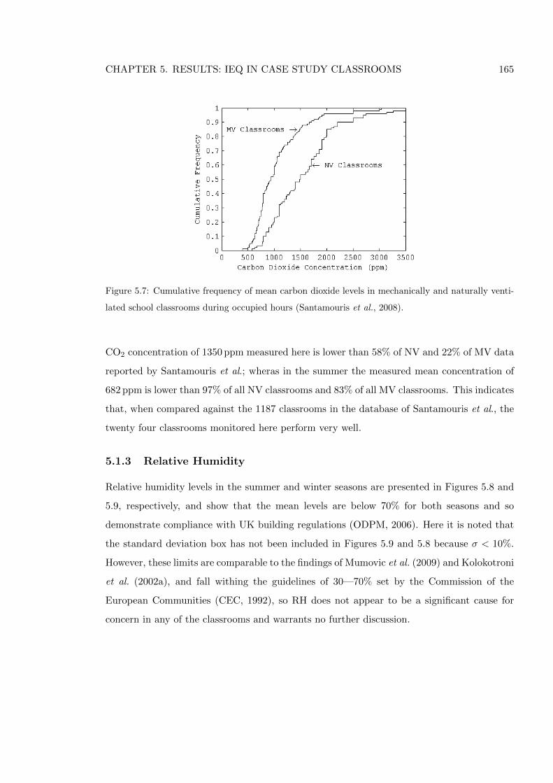
CHAPTER 5. RESULTS: IEQ IN CASE STUDY CLASSROOMS 165
Figure 5.7: Cumulative frequency of mean carbon dioxide levels in mechanically and naturally venti-
lated school classrooms during occupied hours (Santamouris et al., 2008).
CO2 concentration of 1350 ppm measured here is lower than 58% of NV and 22% of MV data
reported by Santamouris et al.; wheras in the summer the measured mean concentration of
682 ppm is lower than 97% of all NV classrooms and 83% of all MV classrooms. This indicates
that, when compared against the 1187 classrooms in the database of Santamouris et al., the
twenty four classrooms monitored here perform very well.
5.1.3 Relative Humidity
Relative humidity levels in the summer and winter seasons are presented in Figures 5.8 and
5.9, respectively, and show that the mean levels are below 70% for both seasons and so
demonstrate compliance with UK building regulations (ODPM, 2006). Here it is noted that
the standard deviation box has not been included in Figures 5.9 and 5.8 because σ < 10%.
However, these limits are comparable to the findings of Mumovic et al. (2009) and Kolokotroni
et al. (2002a), and fall withing the guidelines of 30—70% set by the Commission of the
European Communities (CEC, 1992), so RH does not appear to be a significant cause for
concern in any of the classrooms and warrants no further discussion.
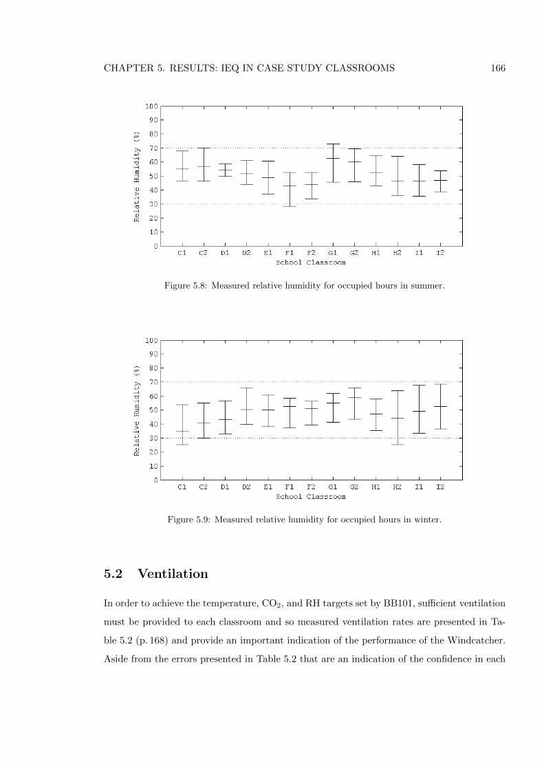
CHAPTER 5. RESULTS: IEQ IN CASE STUDY CLASSROOMS 166
Figure 5.8: Measured relative humidity for occupied hours in summer.
Figure 5.9: Measured relative humidity for occupied hours in winter.
5.2 Ventilation
In order to achieve the temperature, CO2, and RH targets set by BB101, sufficient ventilation
must be provided to each classroom and so measured ventilation rates are presented in Ta-
ble 5.2 (p. 168) and provide an important indication of the performance of the Windcatcher.
Aside from the errors presented in Table 5.2 that are an indication of the confidence in each
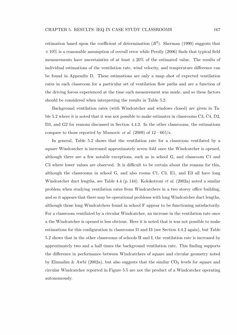
CHAPTER 5. RESULTS: IEQ IN CASE STUDY CLASSROOMS 167
estimation based upon the coefficient of determination (R2). Sherman (1990) suggests that
± 10% is a reasonable assumption of overall error while Persily (2006) finds that typical field
measurements have uncertainties of at least ± 20% of the estimated value. The results of
individual estimations of the ventilation rate, wind velocity, and temperature difference can
be found in Appendix D. These estimations are only a snap–shot of expected ventilation
rates in each classroom for a particular set of ventilation flow paths and are a function of
the driving forces experienced at the time each measurement was made, and so these factors
should be considered when interpreting the results in Table 5.2.
Background ventilation rates (with Windcatcher and windows closed) are given in Ta-
ble 5.2 where it is noted that it was not possible to make estimates in classrooms C3, C4, D2,
D3, and G2 for reasons discussed in Section 4.4.2. In the other classrooms, the estimations
compare to those reported by Mumovic et al. (2009) of 12—60 l/s.
In general, Table 5.2 shows that the ventilation rate for a classroom ventilated by a
square Windcatcher is increased approximately seven–fold once the Windcatcher is opened,
although there are a few notable exceptions, such as in school G, and classroom C1 and
C3 where lower values are observed. It is difficult to be certain about the reasons for this,
although the classrooms in school G, and also rooms C1, C3, E1, and E3 all have long
Windcatcher duct lengths, see Table 4.4 (p. 144). Kolokotroni et al. (2002a) noted a similar
problem when studying ventilation rates from Windcatchers in a two storey office building,
and so it appears that there may be operational problems with long Windcatcher duct lengths,
although those long Windcatchers found in school F appear to be functioning satisfactorily.
For a classroom ventilated by a circular Windcatcher, an increase in the ventilation rate once
a the Windcatcher is opened is less obvious. Here it is noted that is was not possible to make
estimations for this configuration in classrooms I1 and I3 (see Section 4.4.2 again), but Table
5.2 shows that in the other classrooms of schools H and I, the ventilation rate is increased by
approximately two and a half times the background ventilation rate. This finding supports
the difference in performance between Windcatchers of square and circular geometry noted
by Elmualim & Awbi (2002a), but also suggests that the similar CO2 levels for square and
circular Windcatcher reported in Figure 5.5 are not the product of a Windcatcher operating
autonomously.
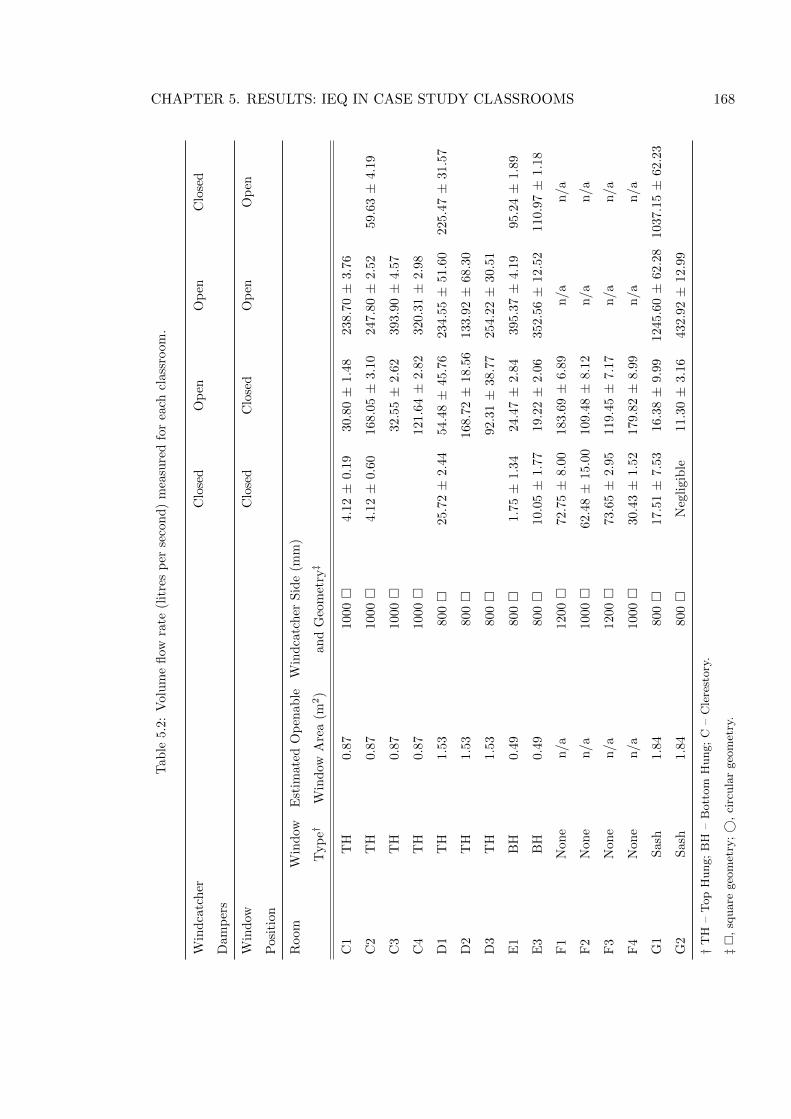
CHAPTER 5. RESULTS: IEQ IN CASE STUDY CLASSROOMS 168
Tab
le5.
2:V
olu
me
flow
rate
(lit
res
per
seco
nd
)m
easu
red
for
each
class
room
.
Win
dca
tch
erC
lose
dO
pen
Op
enC
lose
d
Dam
per
s
Win
dow
Clo
sed
Clo
sed
Op
enO
pen
Pos
itio
n
Room
Win
dow
Est
imat
edO
pen
able
Win
dca
tch
erS
ide
(mm
)
Typ
e†W
ind
owA
rea
(m2)
an
dG
eom
etry‡
C1
TH
0.87
1000�
4.1
2±
0.1
930.8
0±
1.4
8238.7
0±
3.7
6
C2
TH
0.87
1000�
4.1
2±
0.6
0168.0
5±
3.1
0247.8
0±
2.5
259.6
3±
4.1
9
C3
TH
0.87
1000�
32.5
5±
2.6
2393.9
0±
4.5
7
C4
TH
0.87
1000�
121.6
4±
2.8
2320.3
1±
2.9
8
D1
TH
1.53
800�
25.7
2±
2.4
454.4
8±
45.7
623
4.5
5±
51.6
0225.4
7±
31.5
7
D2
TH
1.53
800�
168.7
2±
18.5
6133.9
2±
68.3
0
D3
TH
1.53
800�
92.3
1±
38.7
7254.2
2±
30.5
1
E1
BH
0.49
800�
1.7
5±
1.3
424.4
7±
2.8
4395.3
7±
4.1
995.2
4±
1.8
9
E3
BH
0.49
800�
10.0
5±
1.7
719.2
2±
2.0
635
2.5
6±
12.5
2110.9
7±
1.1
8
F1
Non
en
/a1200�
72.7
5±
8.0
0183.6
9±
6.8
9n
/a
n/a
F2
Non
en
/a1000�
62.4
8±
15.0
0109.4
8±
8.1
2n
/a
n/a
F3
Non
en
/a1200�
73.6
5±
2.9
5119.4
5±
7.1
7n
/a
n/a
F4
Non
en
/a1000�
30.4
3±
1.5
2179.8
2±
8.9
9n
/a
n/a
G1
Sas
h1.
84800�
17.5
1±
7.5
316.3
8±
9.9
912
45.6
0±
62.2
81037.1
5±
62.2
3
G2
Sas
h1.
84800�
Neg
ligib
le11.3
0±
3.1
643
2.9
2±
12.9
9
†T
H–
Top
Hung;
BH
–B
ott
om
Hung;
C–
Cle
rest
ory
.
‡�
,sq
uare
geo
met
ry;©
,ci
rcula
rgeo
met
ry.
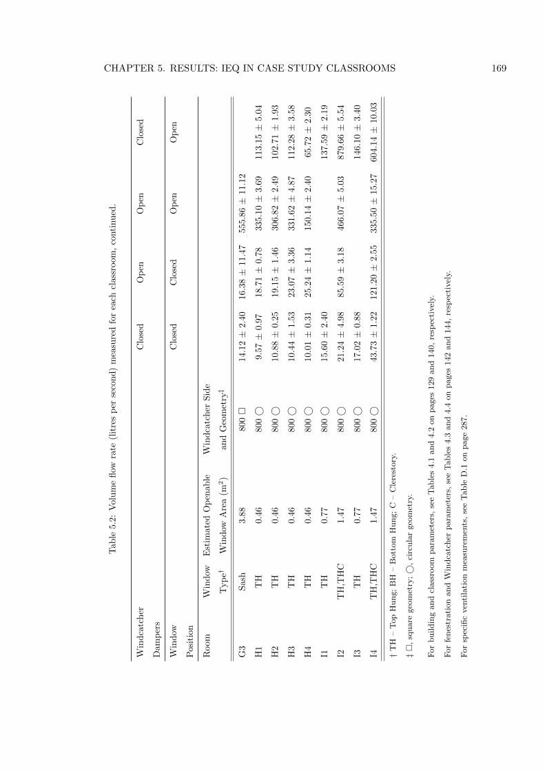
CHAPTER 5. RESULTS: IEQ IN CASE STUDY CLASSROOMS 169
Tab
le5.
2:V
olu
me
flow
rate
(lit
res
per
seco
nd
)m
easu
red
for
each
class
room
,co
nti
nu
ed.
Win
dca
tch
erC
lose
dO
pen
Op
enC
lose
d
Dam
per
s
Win
dow
Clo
sed
Clo
sed
Op
enO
pen
Pos
itio
n
Room
Win
dow
Est
imat
edO
pen
able
Win
dca
tch
erS
ide
Typ
e†W
ind
owA
rea
(m2)
an
dG
eom
etry‡
G3
Sas
h3.
88800�
14.1
2±
2.4
016.3
8±
11.4
7555.8
6±
11.1
2
H1
TH
0.46
800©
9.5
7±
0.9
718.7
1±
0.7
8335.1
0±
3.6
9113.1
5±
5.0
4
H2
TH
0.46
800©
10.8
8±
0.2
519.1
5±
1.4
6306.8
2±
2.4
9102.7
1±
1.9
3
H3
TH
0.46
800©
10.4
4±
1.5
323.0
7±
3.3
6331.6
2±
4.8
7112.2
8±
3.5
8
H4
TH
0.46
800©
10.0
1±
0.3
125.2
4±
1.1
4150.1
4±
2.4
065.7
2±
2.3
0
I1T
H0.
77800©
15.6
0±
2.4
0137.5
9±
2.1
9
I2T
H,T
HC
1.47
800©
21.2
4±
4.9
885.5
9±
3.1
8466.0
7±
5.0
3879.6
6±
5.5
4
I3T
H0.
77800©
17.0
2±
0.8
8146.1
0±
3.4
0
I4T
H,T
HC
1.47
800©
43.7
3±
1.2
2121.2
0±
2.5
5335.5
0±
15.2
7604.1
4±
10.0
3
†T
H–
Top
Hung;
BH
–B
ott
om
Hung;
C–
Cle
rest
ory
.
‡�
,sq
uare
geo
met
ry;©
,ci
rcula
rgeo
met
ry.
For
buildin
gand
class
room
para
met
ers,
see
Table
s4.1
and
4.2
on
pages
129
and
140,
resp
ecti
vel
y.
For
fenes
trati
on
and
Win
dca
tcher
para
met
ers,
see
Table
s4.3
and
4.4
on
pages
142
and
144,
resp
ecti
vel
y.
For
spec
ific
ven
tila
tion
mea
sure
men
ts,
see
Table
D.1
on
page
287.
CHAPTER 5. RESULTS: IEQ IN CASE STUDY CLASSROOMS 170
In Table 5.2, is it evident that by opening windows as well as the Windcatcher it is possible
to significantly increase the ventilation rate in a classroom, but here it is noted that it is not
possible to open the windows in school F. In general, ventilation rates are seen to increase
at least two–fold, although some very high multiples also appear possible, see classroom G1
for example. Here, it is interesting to isolate the effect of the Windcatcher by closing the
dampers and opening the windows. In order to investigate this, specific tests were conducted
in classrooms C1, D1, E1, E3, and G1, as well as all of the classrooms in schools H and I, to
estimate the ventilation through the maximum openable window area with the Windcatcher
closed. Table 5.2 shows that in classrooms C1, E1, E3, and H1–4, with the windows open and
the Windcatcher closed, flow rates were between 64–76% less than the flow rates generated
with the windows and the Windcatcher open, whereas in D1 and G1 flow rates were only
4–16% less. The greater openable window area is the likely explanation for the differences
between these results and this has been demonstrated theoretically in Figure 3.33, which
shows that when the wind speed is constant, the ventilation rate in a room increases with an
increase in window area.
Classrooms I2 and I4 contain a Windcatcher and conventional windows that are aug-
mented by clerestory windows located in the opposite facade, see Table 4.3 (p. 142) and
Figure 2.4 (p. 49). Table 5.3 (p. 171) presents estimated ventilation rates measured for six
different combinations of open or closed Windcatcher, facade windows, and clerestory win-
dows. It shows that the greatest ventilation rate is achieved in these classrooms with the
facade and clerestory windows open and the Windcatcher closed. In fact, the estimated ven-
tilation rate with all windows and the Windcatcher open is approximately 50% less than that
measured for the facade and clerestory windows open and the Windcatcher closed. This sug-
gests that an open Windcatcher interferes with the air flow between the facade and clerestory
windows, although it is unclear why this is so. When the Windcatcher is used in coordination
with either the facade or the clerestory windows the estimated ventilation rate is greater than
those measured when either the facade or the clerestory windows are used exclusively and the
Windcatcher is closed. Table 4.4 (p. 144) shows that the CSA of the circular Windcatchers
found in classrooms I2 and I4 is 0.5 m2, whereas Table 4.3 (p. 142) shows that the facade
and clerestory windows have estimated opening areas of 9.98 m2 and 3.43 m2, respectively.
The combined opening area of both window types far exceeds the opening area provided by a
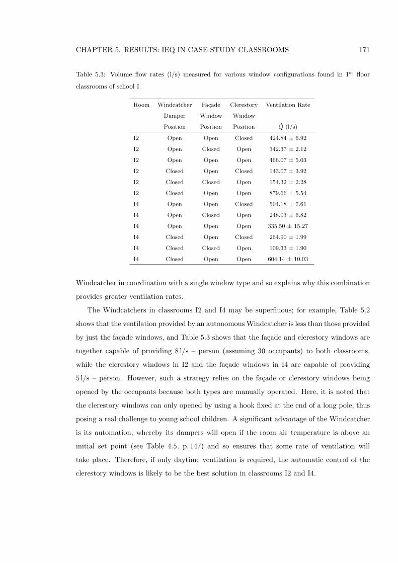
CHAPTER 5. RESULTS: IEQ IN CASE STUDY CLASSROOMS 171
Table 5.3: Volume flow rates (l/s) measured for various window configurations found in 1st floor
classrooms of school I.
Room Windcatcher Facade Clerestory Ventilation Rate
Damper Window Window
Position Position Position Q (l/s)
I2 Open Open Closed 424.84 ± 6.92
I2 Open Closed Open 342.37 ± 2.12
I2 Open Open Open 466.07 ± 5.03
I2 Closed Open Closed 143.07 ± 3.92
I2 Closed Closed Open 154.32 ± 2.28
I2 Closed Open Open 879.66 ± 5.54
I4 Open Open Closed 504.18 ± 7.61
I4 Open Closed Open 248.03 ± 6.82
I4 Open Open Open 335.50 ± 15.27
I4 Closed Open Closed 264.90 ± 1.99
I4 Closed Closed Open 109.33 ± 1.90
I4 Closed Open Open 604.14 ± 10.03
Windcatcher in coordination with a single window type and so explains why this combination
provides greater ventilation rates.
The Windcatchers in classrooms I2 and I4 may be superfluous; for example, Table 5.2
shows that the ventilation provided by an autonomous Windcatcher is less than those provided
by just the facade windows, and Table 5.3 shows that the facade and clerestory windows are
together capable of providing 8 l/s – person (assuming 30 occupants) to both classrooms,
while the clerestory windows in I2 and the facade windows in I4 are capable of providing
5 l/s – person. However, such a strategy relies on the facade or clerestory windows being
opened by the occupants because both types are manually operated. Here, it is noted that
the clerestory windows can only opened by using a hook fixed at the end of a long pole, thus
posing a real challenge to young school children. A significant advantage of the Windcatcher
is its automation, whereby its dampers will open if the room air temperature is above an
initial set point (see Table 4.5, p. 147) and so ensures that some rate of ventilation will
take place. Therefore, if only daytime ventilation is required, the automatic control of the
clerestory windows is likely to be the best solution in classrooms I2 and I4.
CHAPTER 5. RESULTS: IEQ IN CASE STUDY CLASSROOMS 172
The results in Table 5.2 generally indicate that a Windcatcher operating in coordination
with open windows located in a single facade will increase the ventilation rate over and above
those provided by a Windcatcher or windows on their own, and so together provide a viable
method for meeting BB101 ventilation requirements. These findings tally with the findings
of Kirk & Kolokotroni (2004b) who measured flow rates in an office ventilated by several
Windcatchers and found that ventilation rates increase when a Windcatcher operates in
combination with open windows, and that ventilation through windows alone can be greater
than those achieved through an autonomous Windcatcher. However, in this situation, the
use of windows was disliked by the occupants because they caused uncomfortable draughts,
although no such observations were found during the current study.
In order to compare the estimated ventilation rates presented in Table 5.2 against the
requirements of BB101 it is necessary to assume the number of occupants in each classroom.
Here, the design occupancy for each classroom given in Table 4.2 (p. 140) are assumed and
so provide a worst case scenario. Accordingly, the estimated ventilation rates presented
in Figures 5.10—5.12 may under–estimate the actual ventilation rate per person if class
sizes are smaller, which is possible in Secondary schools. Figure 5.10 suggests that the
minimum ventilation rate of 3 l/s – person cannot be met by background ventilation (through
infiltration) alone, except in classrooms F1 and F3 that have a lower occupancy level. When
using a Windcatcher on its own, Figure 5.11 shows that the minimum ventilation rate of
3 l/s – person is met in ten classrooms, and the required mean flow rate of 5 l/s – person
is surpassed in five classrooms. When a Windcatcher is combined with fully open windows,
then Figure 5.12 shows that 5 l/s – person is met in all classrooms except in D2 which is
very close to the required value. It is also evident that the required purge ventilation rate
of 8± 0.2 l/s – person is achieved in all rooms except D2 and I4. Here, there is no clear
explanation for the lower ventilation rates found in these rooms, as the driving forces when
the measurements were made do not differ greatly from those for other rooms, see Table D.1
in Appendix D.
In two similar studies, Mumovic et al. (2009) and Griffiths & Eftekhari (2008) found that
the window area in naturally ventilated schools is insufficient for providing 8 l/s – person,
and Figure 5.13 shows that the ventilation rates provided by single sided ventilation through
open windows also cannot meet this standard. Consequently, Figures 5.10—5.12 (p. 173 and
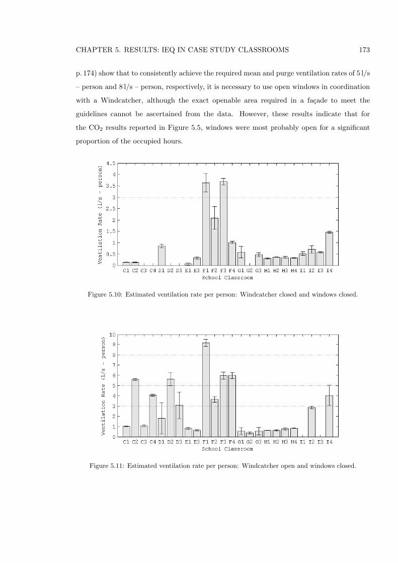
CHAPTER 5. RESULTS: IEQ IN CASE STUDY CLASSROOMS 173
p. 174) show that to consistently achieve the required mean and purge ventilation rates of 5 l/s
– person and 8 l/s – person, respectively, it is necessary to use open windows in coordination
with a Windcatcher, although the exact openable area required in a facade to meet the
guidelines cannot be ascertained from the data. However, these results indicate that for
the CO2 results reported in Figure 5.5, windows were most probably open for a significant
proportion of the occupied hours.
Figure 5.10: Estimated ventilation rate per person: Windcatcher closed and windows closed.
Figure 5.11: Estimated ventilation rate per person: Windcatcher open and windows closed.
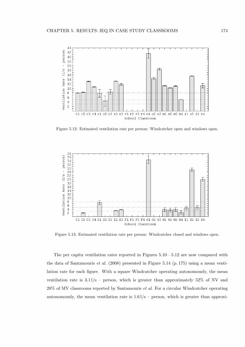
CHAPTER 5. RESULTS: IEQ IN CASE STUDY CLASSROOMS 174
Figure 5.12: Estimated ventilation rate per person: Windcatcher open and windows open.
Figure 5.13: Estimated ventilation rate per person: Windcatcher closed and windows open.
The per capita ventilation rates reported in Figures 5.10—5.12 are now compared with
the data of Santamouris et al. (2008) presented in Figure 5.14 (p. 175) using a mean venti-
lation rate for each figure. With a square Windcatcher operating autonomously, the mean
ventilation rate is 3.1 l/s – person, which is greater than approximately 52% of NV and
28% of MV classrooms reported by Santamouris et al. For a circular Windcatcher operating
autonomously, the mean ventilation rate is 1.6 l/s – person, which is greater than approxi-
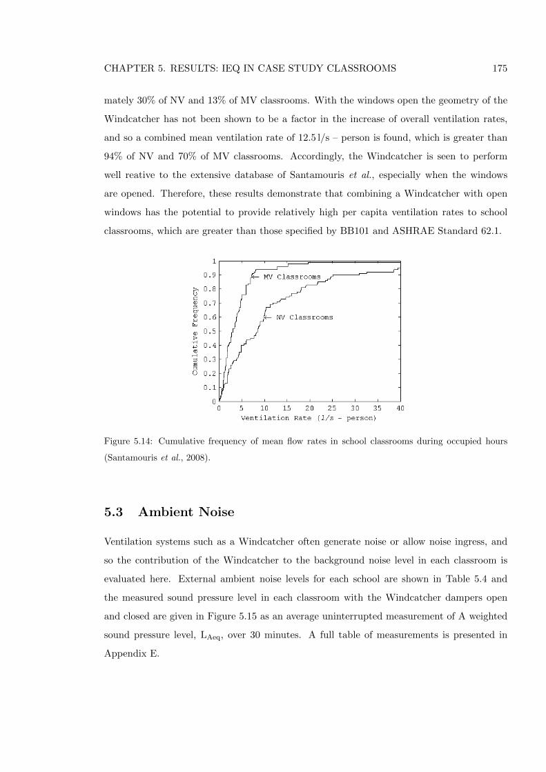
CHAPTER 5. RESULTS: IEQ IN CASE STUDY CLASSROOMS 175
mately 30% of NV and 13% of MV classrooms. With the windows open the geometry of the
Windcatcher has not been shown to be a factor in the increase of overall ventilation rates,
and so a combined mean ventilation rate of 12.5 l/s – person is found, which is greater than
94% of NV and 70% of MV classrooms. Accordingly, the Windcatcher is seen to perform
well reative to the extensive database of Santamouris et al., especially when the windows
are opened. Therefore, these results demonstrate that combining a Windcatcher with open
windows has the potential to provide relatively high per capita ventilation rates to school
classrooms, which are greater than those specified by BB101 and ASHRAE Standard 62.1.
Figure 5.14: Cumulative frequency of mean flow rates in school classrooms during occupied hours
(Santamouris et al., 2008).
5.3 Ambient Noise
Ventilation systems such as a Windcatcher often generate noise or allow noise ingress, and
so the contribution of the Windcatcher to the background noise level in each classroom is
evaluated here. External ambient noise levels for each school are shown in Table 5.4 and
the measured sound pressure level in each classroom with the Windcatcher dampers open
and closed are given in Figure 5.15 as an average uninterrupted measurement of A weighted
sound pressure level, LAeq, over 30 minutes. A full table of measurements is presented in
Appendix E.
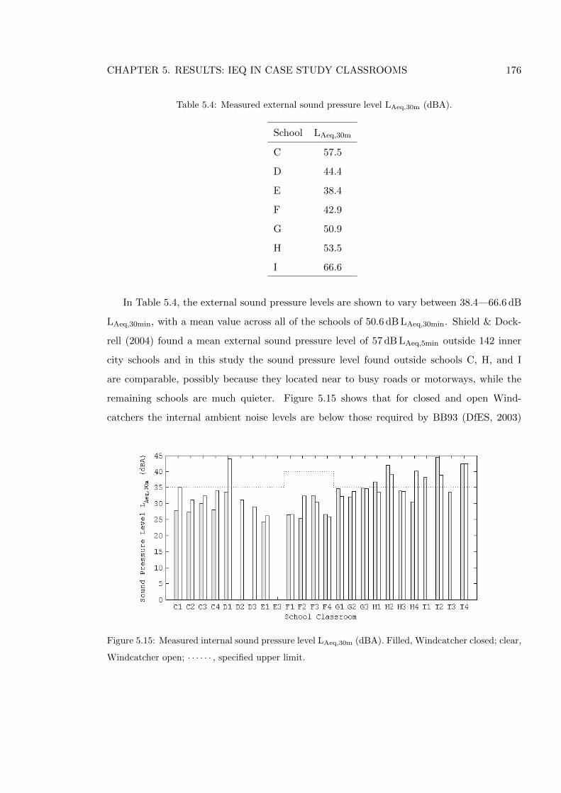
CHAPTER 5. RESULTS: IEQ IN CASE STUDY CLASSROOMS 176
Table 5.4: Measured external sound pressure level LAeq,30m (dBA).
School LAeq,30m
C 57.5
D 44.4
E 38.4
F 42.9
G 50.9
H 53.5
I 66.6
In Table 5.4, the external sound pressure levels are shown to vary between 38.4—66.6 dB
LAeq,30min, with a mean value across all of the schools of 50.6 dB LAeq,30min. Shield & Dock-
rell (2004) found a mean external sound pressure level of 57 dB LAeq,5min outside 142 inner
city schools and in this study the sound pressure level found outside schools C, H, and I
are comparable, possibly because they located near to busy roads or motorways, while the
remaining schools are much quieter. Figure 5.15 shows that for closed and open Wind-
catchers the internal ambient noise levels are below those required by BB93 (DfES, 2003)
Figure 5.15: Measured internal sound pressure level LAeq,30m (dBA). Filled, Windcatcher closed; clear,
Windcatcher open; · · · · · · , specified upper limit.
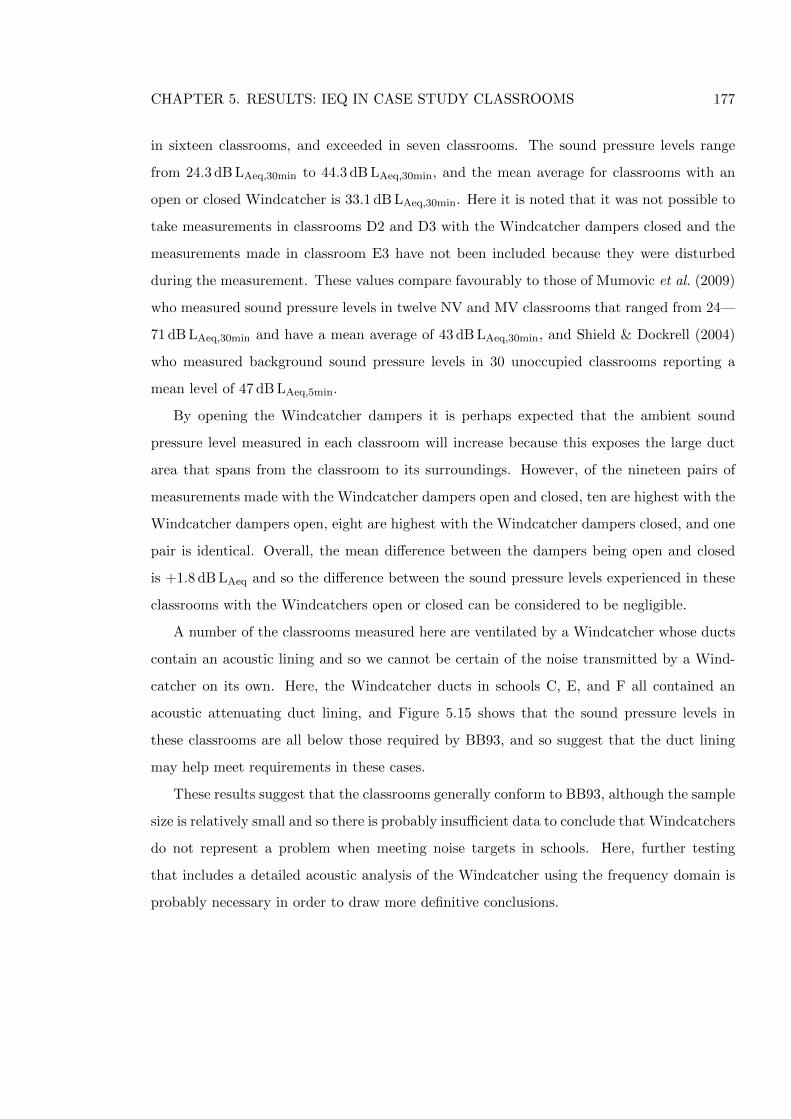
CHAPTER 5. RESULTS: IEQ IN CASE STUDY CLASSROOMS 177
in sixteen classrooms, and exceeded in seven classrooms. The sound pressure levels range
from 24.3 dB LAeq,30min to 44.3 dB LAeq,30min, and the mean average for classrooms with an
open or closed Windcatcher is 33.1 dB LAeq,30min. Here it is noted that it was not possible to
take measurements in classrooms D2 and D3 with the Windcatcher dampers closed and the
measurements made in classroom E3 have not been included because they were disturbed
during the measurement. These values compare favourably to those of Mumovic et al. (2009)
who measured sound pressure levels in twelve NV and MV classrooms that ranged from 24—
71 dB LAeq,30min and have a mean average of 43 dB LAeq,30min, and Shield & Dockrell (2004)
who measured background sound pressure levels in 30 unoccupied classrooms reporting a
mean level of 47 dB LAeq,5min.
By opening the Windcatcher dampers it is perhaps expected that the ambient sound
pressure level measured in each classroom will increase because this exposes the large duct
area that spans from the classroom to its surroundings. However, of the nineteen pairs of
measurements made with the Windcatcher dampers open and closed, ten are highest with the
Windcatcher dampers open, eight are highest with the Windcatcher dampers closed, and one
pair is identical. Overall, the mean difference between the dampers being open and closed
is +1.8 dB LAeq and so the difference between the sound pressure levels experienced in these
classrooms with the Windcatchers open or closed can be considered to be negligible.
A number of the classrooms measured here are ventilated by a Windcatcher whose ducts
contain an acoustic lining and so we cannot be certain of the noise transmitted by a Wind-
catcher on its own. Here, the Windcatcher ducts in schools C, E, and F all contained an
acoustic attenuating duct lining, and Figure 5.15 shows that the sound pressure levels in
these classrooms are all below those required by BB93, and so suggest that the duct lining
may help meet requirements in these cases.
These results suggest that the classrooms generally conform to BB93, although the sample
size is relatively small and so there is probably insufficient data to conclude that Windcatchers
do not represent a problem when meeting noise targets in schools. Here, further testing
that includes a detailed acoustic analysis of the Windcatcher using the frequency domain is
probably necessary in order to draw more definitive conclusions.
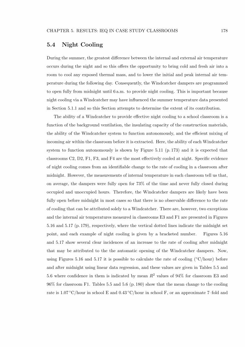
CHAPTER 5. RESULTS: IEQ IN CASE STUDY CLASSROOMS 178
5.4 Night Cooling
During the summer, the greatest difference between the internal and external air temperature
occurs during the night and so this offers the opportunity to bring cold and fresh air into a
room to cool any exposed thermal mass, and to lower the initial and peak internal air tem-
perature during the following day. Consequently, the Windcatcher dampers are programmed
to open fully from midnight until 6 a.m. to provide night cooling. This is important because
night cooling via a Windcatcher may have influenced the summer temperature data presented
in Section 5.1.1 and so this Section attempts to determine the extent of its contribution.
The ability of a Windcatcher to provide effective night cooling to a school classroom is a
function of the background ventilation, the insulating capacity of the construction materials,
the ability of the Windcatcher system to function autonomously, and the efficient mixing of
incoming air within the classroom before it is extracted. Here, the ability of each Windcatcher
system to function autonomously is shown by Figure 5.11 (p. 173) and it is expected that
classrooms C2, D2, F1, F3, and F4 are the most effectively cooled at night. Specific evidence
of night cooling comes from an identifiable change to the rate of cooling in a classroom after
midnight. However, the measurements of internal temperature in each classroom tell us that,
on average, the dampers were fully open for 73% of the time and never fully closed during
occupied and unoccupied hours. Therefore, the Windcatcher dampers are likely have been
fully open before midnight in most cases so that there is no observable difference to the rate
of cooling that can be attributed solely to a Windcatcher. There are, however, two exceptions
and the internal air temperatures measured in classrooms E3 and F1 are presented in Figures
5.16 and 5.17 (p. 179), respectively, where the vertical dotted lines indicate the midnight set
point, and each example of night cooling is given by a bracketed number. Figures 5.16
and 5.17 show several clear incidences of an increase to the rate of cooling after midnight
that may be attributed to the the automatic opening of the Windcatcher dampers. Now,
using Figures 5.16 and 5.17 it is possible to calculate the rate of cooling (◦C/hour) before
and after midnight using linear data regression, and these values are given in Tables 5.5 and
5.6 where confidence in them is indicated by mean R2 values of 94% for classroom E3 and
96% for classroom F1. Tables 5.5 and 5.6 (p. 180) show that the mean change to the cooling
rate is 1.07 ◦C/hour in school E and 0.43 ◦C/hour in school F, or an approximate 7–fold and
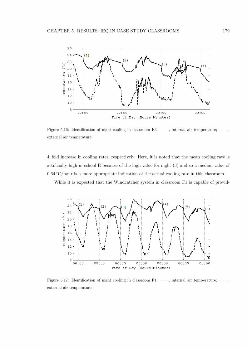
CHAPTER 5. RESULTS: IEQ IN CASE STUDY CLASSROOMS 179
Figure 5.16: Identification of night cooling in classroom E3. ——, internal air temperature; – – –,
external air temperature.
4–fold increase in cooling rates, respectively. Here, it is noted that the mean cooling rate is
artificially high in school E because of the high value for night (3) and so a median value of
0.64 ◦C/hour is a more appropriate indication of the actual cooling rate in this classroom.
While it is expected that the Windcatcher system in classroom F1 is capable of provid-
Figure 5.17: Identification of night cooling in classroom F1. ——, internal air temperature; – – –,
external air temperature.
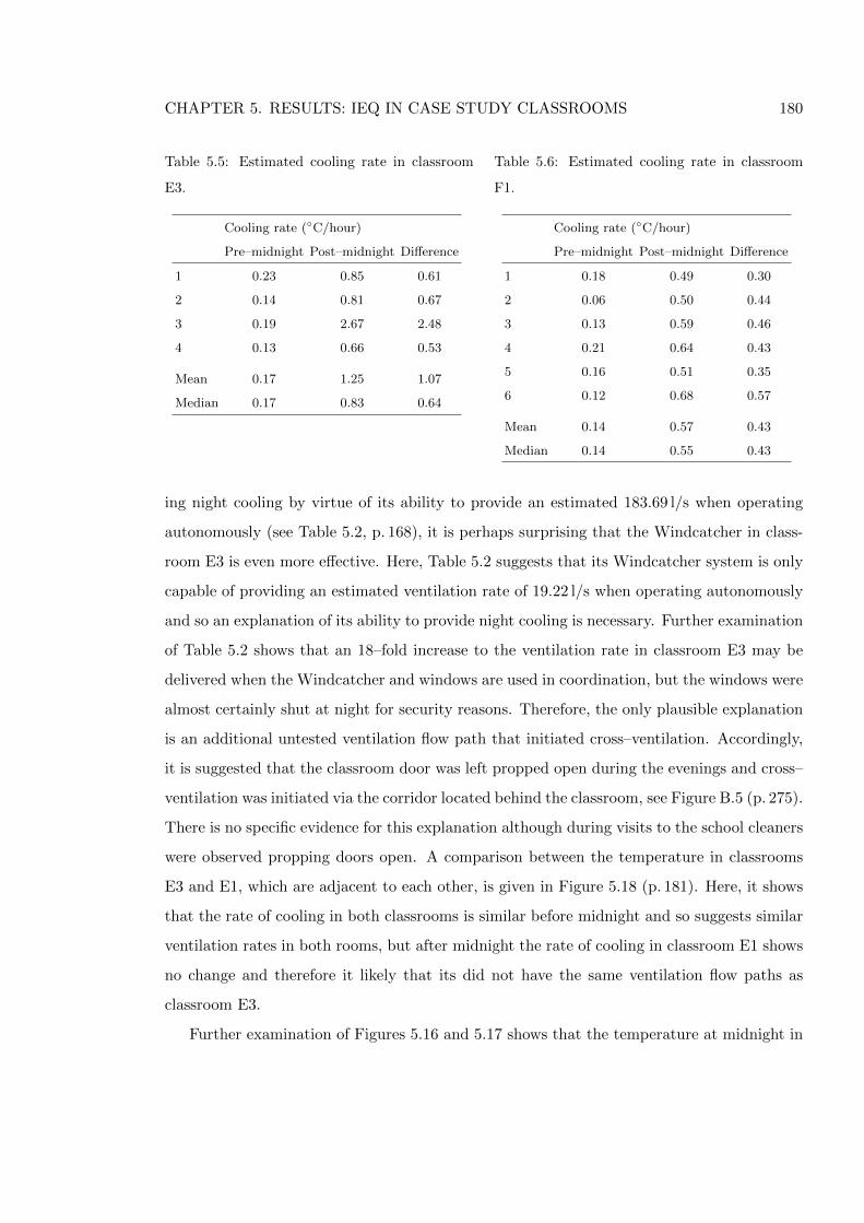
CHAPTER 5. RESULTS: IEQ IN CASE STUDY CLASSROOMS 180
Table 5.5: Estimated cooling rate in classroom
E3.
Cooling rate (◦C/hour)
Pre–midnight Post–midnight Difference
1 0.23 0.85 0.61
2 0.14 0.81 0.67
3 0.19 2.67 2.48
4 0.13 0.66 0.53
Mean 0.17 1.25 1.07
Median 0.17 0.83 0.64
Table 5.6: Estimated cooling rate in classroom
F1.
Cooling rate (◦C/hour)
Pre–midnight Post–midnight Difference
1 0.18 0.49 0.30
2 0.06 0.50 0.44
3 0.13 0.59 0.46
4 0.21 0.64 0.43
5 0.16 0.51 0.35
6 0.12 0.68 0.57
Mean 0.14 0.57 0.43
Median 0.14 0.55 0.43
ing night cooling by virtue of its ability to provide an estimated 183.69 l/s when operating
autonomously (see Table 5.2, p. 168), it is perhaps surprising that the Windcatcher in class-
room E3 is even more effective. Here, Table 5.2 suggests that its Windcatcher system is only
capable of providing an estimated ventilation rate of 19.22 l/s when operating autonomously
and so an explanation of its ability to provide night cooling is necessary. Further examination
of Table 5.2 shows that an 18–fold increase to the ventilation rate in classroom E3 may be
delivered when the Windcatcher and windows are used in coordination, but the windows were
almost certainly shut at night for security reasons. Therefore, the only plausible explanation
is an additional untested ventilation flow path that initiated cross–ventilation. Accordingly,
it is suggested that the classroom door was left propped open during the evenings and cross–
ventilation was initiated via the corridor located behind the classroom, see Figure B.5 (p. 275).
There is no specific evidence for this explanation although during visits to the school cleaners
were observed propping doors open. A comparison between the temperature in classrooms
E3 and E1, which are adjacent to each other, is given in Figure 5.18 (p. 181). Here, it shows
that the rate of cooling in both classrooms is similar before midnight and so suggests similar
ventilation rates in both rooms, but after midnight the rate of cooling in classroom E1 shows
no change and therefore it likely that its did not have the same ventilation flow paths as
classroom E3.
Further examination of Figures 5.16 and 5.17 shows that the temperature at midnight in
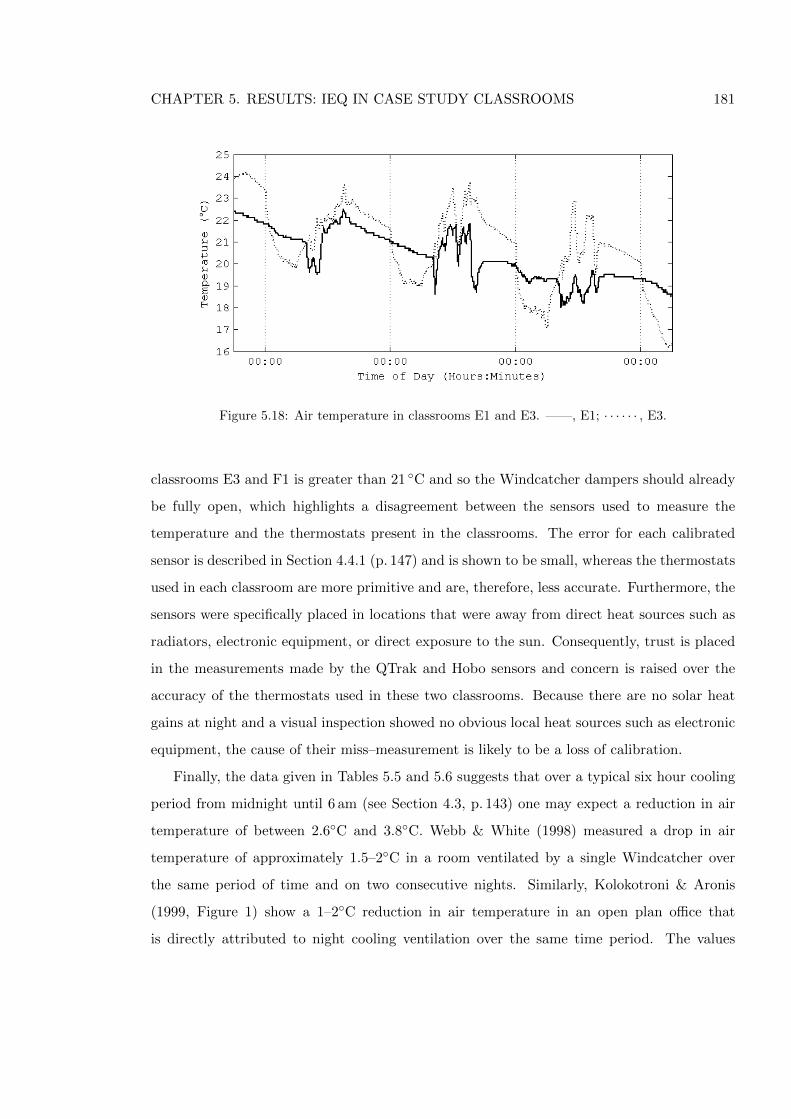
CHAPTER 5. RESULTS: IEQ IN CASE STUDY CLASSROOMS 181
Figure 5.18: Air temperature in classrooms E1 and E3. ——, E1; · · · · · · , E3.
classrooms E3 and F1 is greater than 21 ◦C and so the Windcatcher dampers should already
be fully open, which highlights a disagreement between the sensors used to measure the
temperature and the thermostats present in the classrooms. The error for each calibrated
sensor is described in Section 4.4.1 (p. 147) and is shown to be small, whereas the thermostats
used in each classroom are more primitive and are, therefore, less accurate. Furthermore, the
sensors were specifically placed in locations that were away from direct heat sources such as
radiators, electronic equipment, or direct exposure to the sun. Consequently, trust is placed
in the measurements made by the QTrak and Hobo sensors and concern is raised over the
accuracy of the thermostats used in these two classrooms. Because there are no solar heat
gains at night and a visual inspection showed no obvious local heat sources such as electronic
equipment, the cause of their miss–measurement is likely to be a loss of calibration.
Finally, the data given in Tables 5.5 and 5.6 suggests that over a typical six hour cooling
period from midnight until 6 am (see Section 4.3, p. 143) one may expect a reduction in air
temperature of between 2.6◦C and 3.8◦C. Webb & White (1998) measured a drop in air
temperature of approximately 1.5–2◦C in a room ventilated by a single Windcatcher over
the same period of time and on two consecutive nights. Similarly, Kolokotroni & Aronis
(1999, Figure 1) show a 1–2◦C reduction in air temperature in an open plan office that
is directly attributed to night cooling ventilation over the same time period. The values
CHAPTER 5. RESULTS: IEQ IN CASE STUDY CLASSROOMS 182
given here for the rate of cooling using a Windcatcher are quite high when compared against
those in the literature and suggests that these Windcatchers perform comparatively well.
However, the number of samples is limited and although Figures 5.16 and 5.17 show night
cooling in classrooms E3 and F1, respectively, the true extent of the cooling provided by a
Windcatcher can only be determined by intervention testing that isolates its contribution.
Nevertheless, the evidence of Windcatcher performance presented in this chapter suggests
that it is reasonable to expect Windcatcher systems to deliver ventilation at night if they
are also capable of functioning autonomously. The internal air temperature is lowered if the
external air temperature is lower than the internal temperature and the air mixes well inside
the room. It is then possible to increase cooling rates over and above those delivered by an
autonomous Windcatcher if cross–ventilation can be initiated at night. To improve energy
savings from night ventilation Kolokotroni & Aronis (1999) suggest that a building should be
western facing, the glazing ratio and internal heat gains should be reduced, and air tightness
should be increased.
5.5 Summary
This chapter has reviewed the measurements of IAQ, ventilation, and noise made in twenty
four classrooms of seven UK schools. Results demonstrate that a Windcatcher in coordina-
tion with windows is generally capable of meeting the UK BB101 standard for IAQ and a
Windcatcher can meet the UK BB93 standard for noise.
For the summer months all classrooms were able to meet the CO2 requirements indicating
sufficient per capita ventilation. Measurements of the ventilation rate in each classroom with
a Windcatcher operating autonomously show that 40% of measured classrooms meet the
minimum 3 l/s – person requirement and 23% meet the 5 l/s – person requirement. If the
Windcatcher is used in coordination with open windows, then all classrooms meet the 3 l/s
– person requirement, 94% meet 5 l/s – person, and 77% meet 8 l/s – person under this
arrangement. Furthermore, for the classrooms studied here, it is evident that a Windcatcher
can aid in the delivery of ventilation rates that meet the UK standards during the summer
time and this also extends to meeting European and US standards.
However, the analysis of actual Windcatcher performance shows that it is rarely open
CHAPTER 5. RESULTS: IEQ IN CASE STUDY CLASSROOMS 183
during the winter months and although the maximum CO2 limit of 5000 ppm is never reached,
only 62% of classrooms meet the required mean CO2 level of 1500 ppm and so the control
strategy requires careful revision and is discussed in Chapter 7.
An increase in the rate of cooling at night that can be attributed to a Windcatcher
is shown in two classrooms where the median cooling rate was found to be 0.64◦C/hour
and 0.43◦C/hour. It is reasonable to expect other Windcatcher systems to deliver night
cooling if they are also capable of functioning autonomously, the incoming air mixes well, and
the external air temperature is less than the room air temperature. However, intervention
testing is required to determine the exact contribution of a Windcatcher to a night ventilation
strategy.
Measurements of ambient noise in twenty three classrooms with the Windcatcher dampers
open suggest that the classrooms generally conform to BB93, although the sample size is
relatively small and so there is probably insufficient data to conclude that Windcatchers
do not represent a problem when meeting noise targets in schools. Further work using the
frequency domain is necessary to draw more definitive conclusions and this is described in
Chapter 9.
Finally, a Windcatcher is shown to offer the potential to significantly improve natural
ventilation rates in school classrooms and to help comply with IAQ standards for schools.
CHAPTER 6. RESULTS: PREDICTED AND MEASURED VENTILATION RATES 184
Chapter 6
Results: A Comparison Between
Predicted and Measured
Ventilation Rates
In this chapter, the predictions of the semi–empirical model are compared against experimen-
tal measurements for a Windcatcher operating in–situ to determine its suitability for use in
the design of a natural ventilation strategy that incorporates a Windcatcher. Two cases are
considered: the first is for a Windcatcher functioning autonomously, and the second is for a
Windcatcher in coordination with a single facade opening.
The semi–empirical model uses data measured in the laboratory for the coefficient of
pressure on each face of a 500 mm square Windcatcher, and values for the losses in each
Windcatcher quadrant derived from further laboratory measurements of ventilation rates
through a 500 mm square Windcatcher. Therefore, its predictions can only be compared
against those measurements made for a Windcatcher of similar geometry. Consequently, the
predictions are compared against relevant measurements given in the literature, and because
Section 2.3.2 (p. 63) shows that very little data currently appears in the literature for a Wind-
catcher, measurements made in four schools and twelve classrooms have also been selected
from the case studies described in Chapter 4 to investigate further its performance. Here, all
of the Windcatchers have a square cross–section and a comparable cross sectional area. All of
the Windcatchers considered in this Chapter operate in–situ and so the total losses through
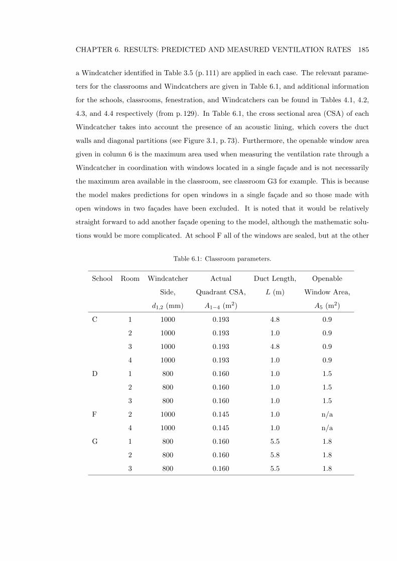
CHAPTER 6. RESULTS: PREDICTED AND MEASURED VENTILATION RATES 185
a Windcatcher identified in Table 3.5 (p. 111) are applied in each case. The relevant parame-
ters for the classrooms and Windcatchers are given in Table 6.1, and additional information
for the schools, classrooms, fenestration, and Windcatchers can be found in Tables 4.1, 4.2,
4.3, and 4.4 respectively (from p. 129). In Table 6.1, the cross sectional area (CSA) of each
Windcatcher takes into account the presence of an acoustic lining, which covers the duct
walls and diagonal partitions (see Figure 3.1, p. 73). Furthermore, the openable window area
given in column 6 is the maximum area used when measuring the ventilation rate through a
Windcatcher in coordination with windows located in a single facade and is not necessarily
the maximum area available in the classroom, see classroom G3 for example. This is because
the model makes predictions for open windows in a single facade and so those made with
open windows in two facades have been excluded. It is noted that it would be relatively
straight forward to add another facade opening to the model, although the mathematic solu-
tions would be more complicated. At school F all of the windows are sealed, but at the other
Table 6.1: Classroom parameters.
School Room Windcatcher Actual Duct Length, Openable
Side, Quadrant CSA, L (m) Window Area,
d1,2 (mm) A1−4 (m2) A5 (m2)
C 1 1000 0.193 4.8 0.9
2 1000 0.193 1.0 0.9
3 1000 0.193 4.8 0.9
4 1000 0.193 1.0 0.9
D 1 800 0.160 1.0 1.5
2 800 0.160 1.0 1.5
3 800 0.160 1.0 1.5
F 2 1000 0.145 1.0 n/a
4 1000 0.145 1.0 n/a
G 1 800 0.160 5.5 1.8
2 800 0.160 5.8 1.8
3 800 0.160 5.5 1.8
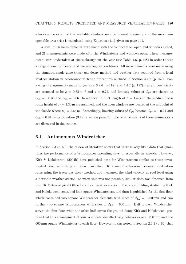
CHAPTER 6. RESULTS: PREDICTED AND MEASURED VENTILATION RATES 186
schools some or all of the available windows may be opened manually and the maximum
openable area (A5) is calculated using Equation (4.1) given on page 141.
A total of 56 measurements were made with the Windcatcher open and windows closed,
and 21 measurements were made with the Windcatcher and windows open. These measure-
ments were undertaken at times throughout the year (see Table 4.6, p. 148) in order to test
a range of environmental and meteorological conditions. All measurements were made using
the standard single–zone tracer gas decay method and weather data acquired from a local
weather station in accordance with the procedures outlined in Section 4.4.2 (p. 152). Fol-
lowing the arguments made in Sections 3.2.6 (p. 118) and 4.4.2 (p. 152), terrain coefficients
are assumed to be k = 0.35 m−a and a = 0.25, and limiting values of Cp5 are chosen as
Cp5 = −0.38 and Cp5 = 0.06. In addition, a duct length of L = 1 m and the median class-
room height of zI = 3.30 m are assumed, and the open windows are located at the midpoint of
the facade where zO = 1.65 m. Accordingly, limiting values of Cp5 become Cp5 = −0.24 and
Cp5 = 0.04 using Equation (3.19) given on page 78. The relative merits of these assumptions
are discussed in due course.
6.1 Autonomous Windcatcher
In Section 2.3 (p. 60), the review of literature shows that there is very little data that quan-
tifies the performance of a Windcatcher operating in–situ, especially in schools. However,
Kirk & Kolokotroni (2004b) have published data for Windcatchers similar to those inves-
tigated here, ventilating an open plan office. Kirk and Kolokotroni measured ventilation
rates using the tracer gas decay method and measured the wind velocity at roof level using
a portable weather station, or when this was not possible, similar data was obtained from
the UK Meteorological Office for a local weather station. The office building studied by Kirk
and Kolokotroni contained four square Windcatchers, and data is published for the first floor
which contained two square Windcatcher elements with sides of d1,2 = 1200 mm and two
further two square Windcatchers with sides of d1,2 = 600 mm. Half of each Windcatcher
serves the first floor while the other half serves the ground floor; Kirk and Kolokotroni pro-
pose that this arrangement of four Windcatchers effectively behaves as one 1200 mm and one
600 mm square Windcatcher to each floor. However, it was noted in Section 2.3.3 (p. 69) that
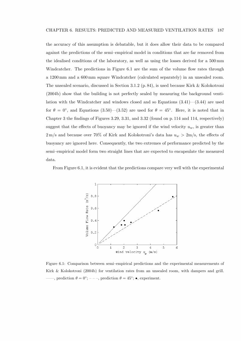
CHAPTER 6. RESULTS: PREDICTED AND MEASURED VENTILATION RATES 187
the accuracy of this assumption is debatable, but it does allow their data to be compared
against the predictions of the semi–empirical model in conditions that are far removed from
the idealised conditions of the laboratory, as well as using the losses derived for a 500 mm
Windcatcher. The predictions in Figure 6.1 are the sum of the volume flow rates through
a 1200 mm and a 600 mm square Windcatcher (calculated separately) in an unsealed room.
The unsealed scenario, discussed in Section 3.1.2 (p. 84), is used because Kirk & Kolokotroni
(2004b) show that the building is not perfectly sealed by measuring the background venti-
lation with the Windcatcher and windows closed and so Equations (3.41)—(3.44) are used
for θ = 0◦, and Equations (3.50)—(3.52) are used for θ = 45◦. Here, it is noted that in
Chapter 3 the findings of Figures 3.29, 3.31, and 3.32 (found on p. 114 and 114, respectively)
suggest that the effects of buoyancy may be ignored if the wind velocity uw, is greater than
2 m/s and because over 70% of Kirk and Kolokotroni’s data has uw > 2m/s, the effects of
buoyancy are ignored here. Consequently, the two extremes of performance predicted by the
semi–empirical model form two straight lines that are expected to encapsulate the measured
data.
From Figure 6.1, it is evident that the predictions compare very well with the experimental
Figure 6.1: Comparison between semi–empirical predictions and the experimental measurements of
Kirk & Kolokotroni (2004b) for ventilation rates from an unsealed room, with dampers and grill.
——, prediction θ = 0◦; – – –, prediction θ = 45◦; •, experiment.
CHAPTER 6. RESULTS: PREDICTED AND MEASURED VENTILATION RATES 188
measurements, particularly for lower wind velocities (uw < 3m/s), although one may argue
that this level of agreement is fortuitous. The wind direction is assumed to have varied
during the measurements and so cannot be said to be at θ = 0◦ or θ = 45◦, although the
measurements agree better with the predictions when θ = 45◦ (average error of 19%) than
when θ = 0◦ (average error 41%). However, the results suggest that there is some merit in
using the values for Cp and K determined from a square 500 mm Windcatcher to predict the
performance of a square Windcatcher of other dimensions, but one cannot expect such good
agreement all of the time, and so the predictions of the semi–empirical model must only be
used as an estimate of true Windcatcher performance. Nevertheless, the predictions obtained
for θ = 0◦ and θ = 45◦ both lie within a reasonable distance of the measured data, and so
it seems sensible to use these as limiting cases where θ = 0◦ represents the best possible
performance, and θ = 45◦ represents an estimation of a worst case performance.
The predictions of the semi–empirical model are now compared against the experimental
measurements made in–situ for this study. All measurements of ventilation rates are given
in Appendix D (p. 287), and for a Windcatcher operating autonomously, the predicted and
measured ventilation rates are presented for 800 mm and 1000 mm Windcatchers in Figures
6.2 and 6.3 for the classrooms given in Table 6.1. The ventilation rates presented in Table 5.2
Figure 6.2: Ventilation rates for an autonomous 800 mm square Windcatcher. ——, prediction θ = 0◦;
– – –, prediction θ = 45◦; •, measurement L ≤ 1 m; ×, measurement L > 1 m.
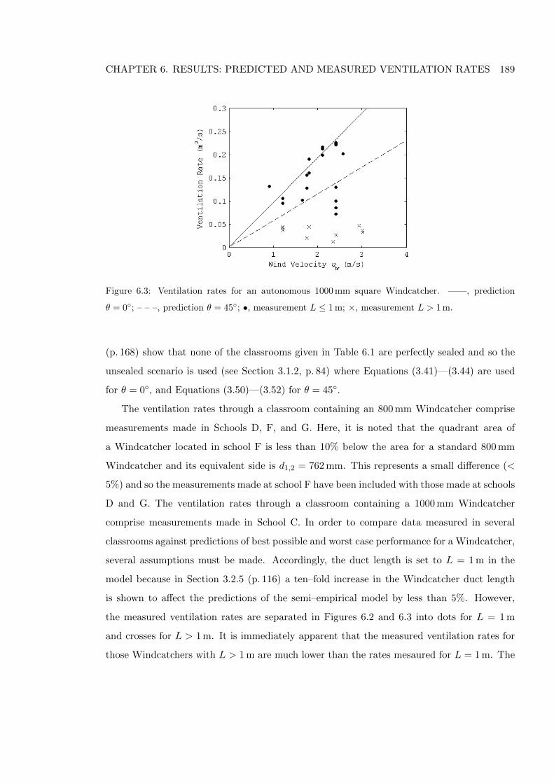
CHAPTER 6. RESULTS: PREDICTED AND MEASURED VENTILATION RATES 189
Figure 6.3: Ventilation rates for an autonomous 1000 mm square Windcatcher. ——, prediction
θ = 0◦; – – –, prediction θ = 45◦; •, measurement L ≤ 1 m; ×, measurement L > 1 m.
(p. 168) show that none of the classrooms given in Table 6.1 are perfectly sealed and so the
unsealed scenario is used (see Section 3.1.2, p. 84) where Equations (3.41)—(3.44) are used
for θ = 0◦, and Equations (3.50)—(3.52) for θ = 45◦.
The ventilation rates through a classroom containing an 800 mm Windcatcher comprise
measurements made in Schools D, F, and G. Here, it is noted that the quadrant area of
a Windcatcher located in school F is less than 10% below the area for a standard 800 mm
Windcatcher and its equivalent side is d1,2 = 762 mm. This represents a small difference (<
5%) and so the measurements made at school F have been included with those made at schools
D and G. The ventilation rates through a classroom containing a 1000 mm Windcatcher
comprise measurements made in School C. In order to compare data measured in several
classrooms against predictions of best possible and worst case performance for a Windcatcher,
several assumptions must be made. Accordingly, the duct length is set to L = 1 m in the
model because in Section 3.2.5 (p. 116) a ten–fold increase in the Windcatcher duct length
is shown to affect the predictions of the semi–empirical model by less than 5%. However,
the measured ventilation rates are separated in Figures 6.2 and 6.3 into dots for L = 1 m
and crosses for L > 1 m. It is immediately apparent that the measured ventilation rates for
those Windcatchers with L > 1 m are much lower than the rates mesaured for L = 1 m. The
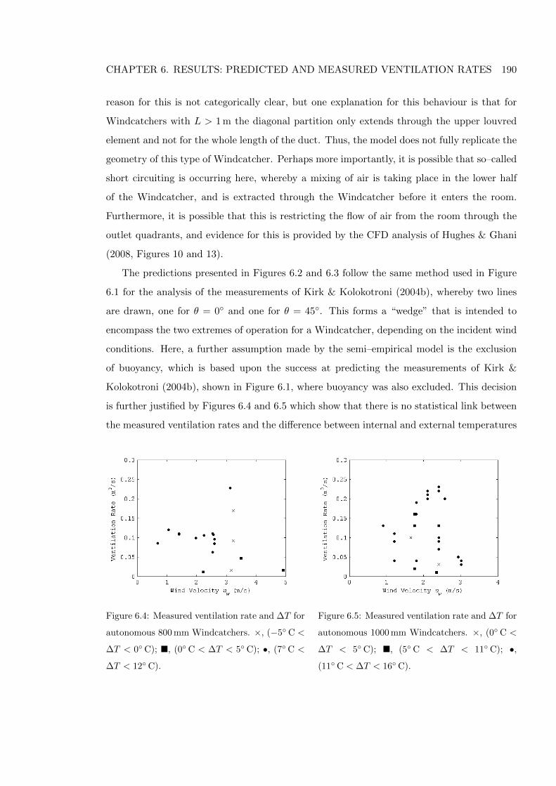
CHAPTER 6. RESULTS: PREDICTED AND MEASURED VENTILATION RATES 190
reason for this is not categorically clear, but one explanation for this behaviour is that for
Windcatchers with L > 1 m the diagonal partition only extends through the upper louvred
element and not for the whole length of the duct. Thus, the model does not fully replicate the
geometry of this type of Windcatcher. Perhaps more importantly, it is possible that so–called
short circuiting is occurring here, whereby a mixing of air is taking place in the lower half
of the Windcatcher, and is extracted through the Windcatcher before it enters the room.
Furthermore, it is possible that this is restricting the flow of air from the room through the
outlet quadrants, and evidence for this is provided by the CFD analysis of Hughes & Ghani
(2008, Figures 10 and 13).
The predictions presented in Figures 6.2 and 6.3 follow the same method used in Figure
6.1 for the analysis of the measurements of Kirk & Kolokotroni (2004b), whereby two lines
are drawn, one for θ = 0◦ and one for θ = 45◦. This forms a “wedge” that is intended to
encompass the two extremes of operation for a Windcatcher, depending on the incident wind
conditions. Here, a further assumption made by the semi–empirical model is the exclusion
of buoyancy, which is based upon the success at predicting the measurements of Kirk &
Kolokotroni (2004b), shown in Figure 6.1, where buoyancy was also excluded. This decision
is further justified by Figures 6.4 and 6.5 which show that there is no statistical link between
the measured ventilation rates and the difference between internal and external temperatures
Figure 6.4: Measured ventilation rate and ∆T for
autonomous 800 mm Windcatchers. ×, (−5◦ C <
∆T < 0◦C); �, (0◦C < ∆T < 5◦C); •, (7◦ C <
∆T < 12◦C).
Figure 6.5: Measured ventilation rate and ∆T for
autonomous 1000 mm Windcatchers. ×, (0◦ C <
∆T < 5◦C); �, (5◦C < ∆T < 11◦ C); •,
(11◦C < ∆T < 16◦C).
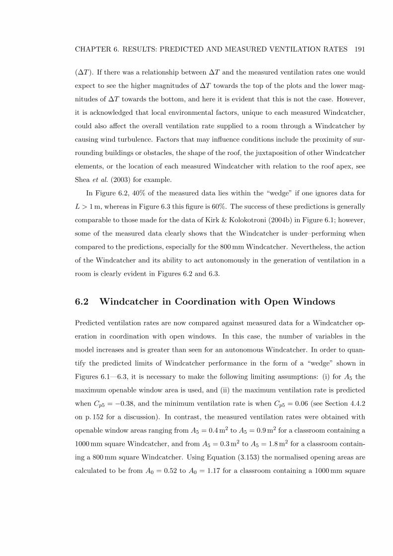
CHAPTER 6. RESULTS: PREDICTED AND MEASURED VENTILATION RATES 191
(∆T ). If there was a relationship between ∆T and the measured ventilation rates one would
expect to see the higher magnitudes of ∆T towards the top of the plots and the lower mag-
nitudes of ∆T towards the bottom, and here it is evident that this is not the case. However,
it is acknowledged that local environmental factors, unique to each measured Windcatcher,
could also affect the overall ventilation rate supplied to a room through a Windcatcher by
causing wind turbulence. Factors that may influence conditions include the proximity of sur-
rounding buildings or obstacles, the shape of the roof, the juxtaposition of other Windcatcher
elements, or the location of each measured Windcatcher with relation to the roof apex, see
Shea et al. (2003) for example.
In Figure 6.2, 40% of the measured data lies within the “wedge” if one ignores data for
L > 1 m, whereas in Figure 6.3 this figure is 60%. The success of these predictions is generally
comparable to those made for the data of Kirk & Kolokotroni (2004b) in Figure 6.1; however,
some of the measured data clearly shows that the Windcatcher is under–performing when
compared to the predictions, especially for the 800 mm Windcatcher. Nevertheless, the action
of the Windcatcher and its ability to act autonomously in the generation of ventilation in a
room is clearly evident in Figures 6.2 and 6.3.
6.2 Windcatcher in Coordination with Open Windows
Predicted ventilation rates are now compared against measured data for a Windcatcher op-
eration in coordination with open windows. In this case, the number of variables in the
model increases and is greater than seen for an autonomous Windcatcher. In order to quan-
tify the predicted limits of Windcatcher performance in the form of a “wedge” shown in
Figures 6.1—6.3, it is necessary to make the following limiting assumptions: (i) for A5 the
maximum openable window area is used, and (ii) the maximum ventilation rate is predicted
when Cp5 = −0.38, and the minimum ventilation rate is when Cp5 = 0.06 (see Section 4.4.2
on p. 152 for a discussion). In contrast, the measured ventilation rates were obtained with
openable window areas ranging from A5 = 0.4 m2 to A5 = 0.9 m2 for a classroom containing a
1000 mm square Windcatcher, and from A5 = 0.3 m2 to A5 = 1.8 m2 for a classroom contain-
ing a 800 mm square Windcatcher. Using Equation (3.153) the normalised opening areas are
calculated to be from A0 = 0.52 to A0 = 1.17 for a classroom containing a 1000 mm square
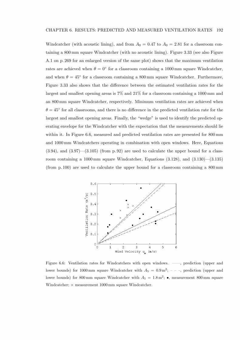
CHAPTER 6. RESULTS: PREDICTED AND MEASURED VENTILATION RATES 192
Windcatcher (with acoustic lining), and from A0 = 0.47 to A0 = 2.81 for a classroom con-
taining a 800 mm square Windcatcher (with no acoustic lining). Figure 3.33 (see also Figure
A.1 on p. 269 for an enlarged version of the same plot) shows that the maximum ventilation
rates are achieved when θ = 0◦ for a classroom containing a 1000 mm square Windcatcher,
and when θ = 45◦ for a classroom containing a 800 mm square Windcatcher. Furthermore,
Figure 3.33 also shows that the difference between the estimated ventilation rates for the
largest and smallest opening areas is 7% and 21% for a classroom containing a 1000 mm and
an 800 mm square Windcatcher, respectively. Minimum ventilation rates are achieved when
θ = 45◦ for all classrooms, and there is no difference in the predicted ventilation rate for the
largest and smallest opening areas. Finally, the “wedge” is used to identify the predicted op-
erating envelope for the Windcatcher with the expectation that the measurements should lie
within it. In Figure 6.6, measured and predicted ventilation rates are presented for 800 mm
and 1000 mm Windcatchers operating in combination with open windows. Here, Equations
(3.94), and (3.97)—(3.105) (from p. 92) are used to calculate the upper bound for a class-
room containing a 1000 mm square Windcatcher, Equations (3.128), and (3.130)—(3.135)
(from p. 100) are used to calculate the upper bound for a classroom containing a 800 mm
Figure 6.6: Ventilation rates for Windcatchers with open windows. ——, prediction (upper and
lower bounds) for 1000 mm square Windcatcher with A5 = 0.9 m2; – – –, prediction (upper and
lower bounds) for 800 mm square Windcatcher with A5 = 1.8 m2; •, measurement 800 mm square
Windcatcher; × measurement 1000 mm square Windcatcher.
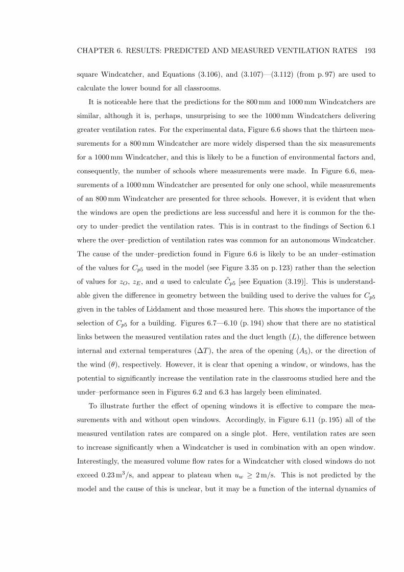
CHAPTER 6. RESULTS: PREDICTED AND MEASURED VENTILATION RATES 193
square Windcatcher, and Equations (3.106), and (3.107)—(3.112) (from p. 97) are used to
calculate the lower bound for all classrooms.
It is noticeable here that the predictions for the 800 mm and 1000 mm Windcatchers are
similar, although it is, perhaps, unsurprising to see the 1000 mm Windcatchers delivering
greater ventilation rates. For the experimental data, Figure 6.6 shows that the thirteen mea-
surements for a 800 mm Windcatcher are more widely dispersed than the six measurements
for a 1000 mm Windcatcher, and this is likely to be a function of environmental factors and,
consequently, the number of schools where measurements were made. In Figure 6.6, mea-
surements of a 1000 mm Windcatcher are presented for only one school, while measurements
of an 800 mm Windcatcher are presented for three schools. However, it is evident that when
the windows are open the predictions are less successful and here it is common for the the-
ory to under–predict the ventilation rates. This is in contrast to the findings of Section 6.1
where the over–prediction of ventilation rates was common for an autonomous Windcatcher.
The cause of the under–prediction found in Figure 6.6 is likely to be an under–estimation
of the values for Cp5 used in the model (see Figure 3.35 on p. 123) rather than the selection
of values for zO, zE , and a used to calculate Cp5 [see Equation (3.19)]. This is understand-
able given the difference in geometry between the building used to derive the values for Cp5
given in the tables of Liddament and those measured here. This shows the importance of the
selection of Cp5 for a building. Figures 6.7—6.10 (p. 194) show that there are no statistical
links between the measured ventilation rates and the duct length (L), the difference between
internal and external temperatures (∆T ), the area of the opening (A5), or the direction of
the wind (θ), respectively. However, it is clear that opening a window, or windows, has the
potential to significantly increase the ventilation rate in the classrooms studied here and the
under–performance seen in Figures 6.2 and 6.3 has largely been eliminated.
To illustrate further the effect of opening windows it is effective to compare the mea-
surements with and without open windows. Accordingly, in Figure 6.11 (p. 195) all of the
measured ventilation rates are compared on a single plot. Here, ventilation rates are seen
to increase significantly when a Windcatcher is used in combination with an open window.
Interestingly, the measured volume flow rates for a Windcatcher with closed windows do not
exceed 0.23 m3/s, and appear to plateau when uw ≥ 2 m/s. This is not predicted by the
model and the cause of this is unclear, but it may be a function of the internal dynamics of
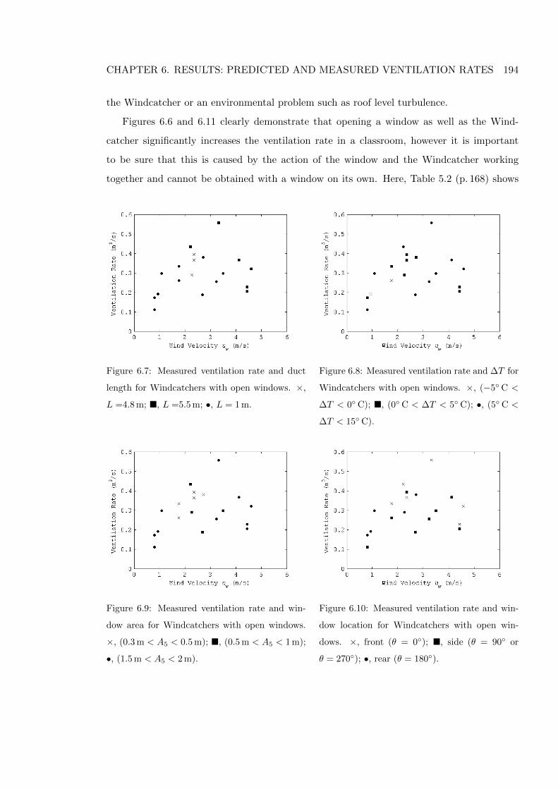
CHAPTER 6. RESULTS: PREDICTED AND MEASURED VENTILATION RATES 194
the Windcatcher or an environmental problem such as roof level turbulence.
Figures 6.6 and 6.11 clearly demonstrate that opening a window as well as the Wind-
catcher significantly increases the ventilation rate in a classroom, however it is important
to be sure that this is caused by the action of the window and the Windcatcher working
together and cannot be obtained with a window on its own. Here, Table 5.2 (p. 168) shows
Figure 6.7: Measured ventilation rate and duct
length for Windcatchers with open windows. ×,
L =4.8 m; �, L =5.5 m; •, L = 1 m.
Figure 6.8: Measured ventilation rate and ∆T for
Windcatchers with open windows. ×, (−5◦C <
∆T < 0◦C); �, (0◦C < ∆T < 5◦ C); •, (5◦C <
∆T < 15◦ C).
Figure 6.9: Measured ventilation rate and win-
dow area for Windcatchers with open windows.
×, (0.3 m < A5 < 0.5 m); �, (0.5 m < A5 < 1 m);
•, (1.5 m < A5 < 2 m).
Figure 6.10: Measured ventilation rate and win-
dow location for Windcatchers with open win-
dows. ×, front (θ = 0◦); �, side (θ = 90◦ or
θ = 270◦); •, rear (θ = 180◦).
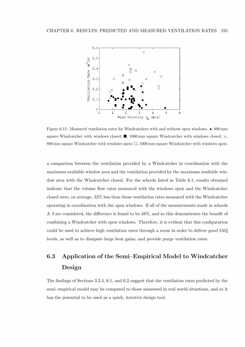
CHAPTER 6. RESULTS: PREDICTED AND MEASURED VENTILATION RATES 195
Figure 6.11: Measured ventilation rates for Windcatchers with and without open windows. •, 800 mm
square Windcatcher with windows closed; �, 1000 mm square Windcatcher with windows closed; ×,
800 mm square Windcatcher with windows open; �, 1000 mm square Windcatcher with windows open.
a comparison between the ventilation provided by a Windcatcher in coordination with the
maximum available window area and the ventilation provided by the maximum available win-
dow area with the Windcatcher closed. For the schools listed in Table 6.1, results obtained
indicate that the volume flow rates measured with the windows open and the Windcatcher
closed were, on average, 32% less than those ventilation rates measured with the Windcatcher
operating in coordination with the open windows. If all of the measurements made in schools
A–I are considered, the difference is found to be 48%, and so this demonstrates the benefit of
combining a Windcatcher with open windows. Therefore, it is evident that this configuration
could be used to achieve high ventilation rates through a room in order to deliver good IAQ
levels, as well as to dissipate large heat gains, and provide purge ventilation rates.
6.3 Application of the Semi–Empirical Model to Windcatcher
Design
The findings of Sections 3.2.4, 6.1, and 6.2 suggest that the ventilation rates predicted by the
semi–empirical model may be compared to those measured in real world situations, and so it
has the potential to be used as a quick, iterative design tool.
CHAPTER 6. RESULTS: PREDICTED AND MEASURED VENTILATION RATES 196
In Section 4.1 (p. 128), climatic conditions are given for each of the case studies discussed
in this chapter, and in Chapter 5, to show the wind velocity expected at each location. Cal-
culations were made using the CIBSE Test Reference Year (TRY) database (CIBSE, 2005b)
which is a synthesised typical weather year suitable for analysing environmental performance
where relevant parameters are given hourly. The given wind speeds can, therefore, be consid-
ered to be steady–state values that are easily applicable to the semi–empirical model because
a key assumption is that it predicts steady–state ventilation scenarios, see Section 3.1 (p. 73).
Therefore, further validation of the semi–empirical model may be achieved by applying the
wind parameters given by the TRY to predict the ventilation rate expected in a specific region.
For example, this can be done using the parameters for a classroom assigned in Sections 6.1
and 6.2, where L = 1 m, zI = 3.30 m, zO = 1.65 m, k = 0.35 m−a and a = 0.25 for an urban
environment. The TRY wind speed is converted to an estimated wind speed at Windcatcher
height using Equation (3.18), here zE = 4.30 m (comparable to School D), and the appro-
priate continuity and flow equations are selected by considering the wind direction, which
is also given by the TRY database. If the Windcatcher is oriented so that each of its faces
are at the four cardinal points (0◦, 90◦, 180◦, and 270◦), then the wind is considered to be
incident to the Windcatcher at θ = 0◦ if it originates from the direction of the cardinal points
± 22.5◦, otherwise it is considered to be incident at θ = 45◦. Therefore, for an autonomous
Windcatcher ventilating an unsealed room, Equations (3.41)—(3.44) are used for θ = 0◦ and
Equations (3.50)—(3.52) are used for θ = 45◦. In Figure 6.12 (p. 197), the TRY for London
Heathrow Airport is used to predict ventilation rates in a classroom ventilated by an 800 mm
Windcatcher and located in an urban area of the south–east of England. Here, the central
bar denotes the mean value, the upper and lower bars denote the maximum and minimum
values, respectively, the dotted boxe denotes one standard deviation (σ) from the mean, and
the three horizontal dotted lines denote the minimum, mean, and purge ventilation rates of
0.09, 0.15, and 0.24 m3/s required by BB101 (DfES, 2006) if a class size of 30 occupants is
assumed. Figure 6.12 shows that an 800 mm Windcatcher is likely to be able to meet the
minimum ventilation requirement, but cannot meet the mean ventilation rate of 0.15 m3/s.
A further calculation for occupied hours [defined as 0900—1530 hrs (DfES, 2006)] is given in
Figure 6.13 (p. 197) and shows that the ventilation rates supplied by an 800 mm Windcatcher
are 16% greater annually and 17% greater during the non–heating season (see Section 2.1.3
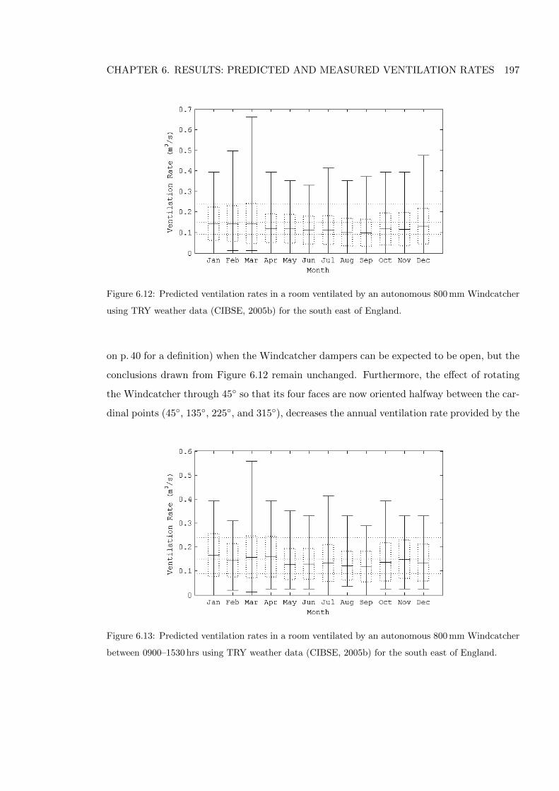
CHAPTER 6. RESULTS: PREDICTED AND MEASURED VENTILATION RATES 197
Figure 6.12: Predicted ventilation rates in a room ventilated by an autonomous 800 mm Windcatcher
using TRY weather data (CIBSE, 2005b) for the south east of England.
on p. 40 for a definition) when the Windcatcher dampers can be expected to be open, but the
conclusions drawn from Figure 6.12 remain unchanged. Furthermore, the effect of rotating
the Windcatcher through 45◦ so that its four faces are now oriented halfway between the car-
dinal points (45◦, 135◦, 225◦, and 315◦), decreases the annual ventilation rate provided by the
Figure 6.13: Predicted ventilation rates in a room ventilated by an autonomous 800 mm Windcatcher
between 0900–1530 hrs using TRY weather data (CIBSE, 2005b) for the south east of England.
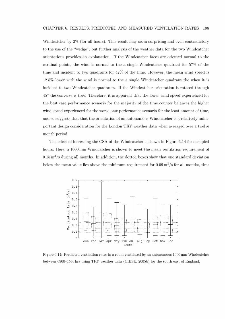
CHAPTER 6. RESULTS: PREDICTED AND MEASURED VENTILATION RATES 198
Windcatcher by 2% (for all hours). This result may seem surprising and even contradictory
to the use of the “wedge”, but further analysis of the weather data for the two Windcatcher
orientations provides an explanation. If the Windcatcher faces are oriented normal to the
cardinal points, the wind is normal to the a single Windcatcher quadrant for 57% of the
time and incident to two quadrants for 47% of the time. However, the mean wind speed is
12.5% lower with the wind is normal to the a single Windcatcher quadrant the when it is
incident to two Windcatcher quadrants. If the Windcatcher orientation is rotated through
45◦ the converse is true. Therefore, it is apparent that the lower wind speed experienced for
the best case performance scenario for the majority of the time counter balances the higher
wind speed experienced for the worse case performance scenario for the least amount of time,
and so suggests that that the orientation of an autonomous Windcatcher is a relatively unim-
portant design consideration for the London TRY weather data when averaged over a twelve
month period.
The effect of increasing the CSA of the Windcatcher is shown in Figure 6.14 for occupied
hours. Here, a 1000 mm Windcatcher is shown to meet the mean ventilation requirement of
0.15 m3/s during all months. In addition, the dotted boxes show that one standard deviation
below the mean value lies above the minimum requirement for 0.09 m3/s for all months, thus
Figure 6.14: Predicted ventilation rates in a room ventilated by an autonomous 1000 mm Windcatcher
between 0900–1530 hrs using TRY weather data (CIBSE, 2005b) for the south east of England.
CHAPTER 6. RESULTS: PREDICTED AND MEASURED VENTILATION RATES 199
suggesting that this requirement is likely to be met using the wind alone for approximately
84% of the time [assuming that 68% of data lies ±σ from the mean value and a further 16%
of all data also lies above the mean value (Ross, 2004)] if the Windcatcher volume control
dampers are fully open. The predictions presented in Figures 6.13 and 6.14 are for the south
east of England and so should be comparable to measurements made in–situ of ventilation
over time, indicated by internal CO2 concentration for the classrooms measured in this study
(see 5.5 5.6 from p. 162). However, a comparison is complicated by the the temperature based
control strategy that is shown in Figure 5.4 (p. 160) to close the volume control dampers in
the winter reducing ventilation rates below those that are actually obtainable, while in the
summer Section 5.1.1 (p. 158) shows that available windows are very likely to be open, thus
increasing the ventilation rates beyond those that can be achieved through an autonomous
Windcatcher. Nevertheless, Figure 6.14 does show that during the heating season (October
to April) the volume control dampers would have to remain fully open for a significant
proportion of occupied hours in order to meet the mean ventilation requirement of BB101.
This would, of course, increase energy losses and the need for additional heating, as well as
the risk of thermal discomfort among occupants located in the draught–risk zone (see Schild,
2004) when cold air is brought into the room through the Windcatcher. These risks are
discussed further in Chapter 7.
BB101 stipulates a purge ventilation rate of 8 l/s – person, which for a classroom of
30 occupants equates to a total ventilation rate of 0.24 m3/s. Figure 6.14 shows that an
average ventilation rate of 0.24 m3/s can be met in January, March, and April using an
autonomous Windcatcher but at other times of the year it can only be achieved using a
Windcatcher in coordination with open windows. Here, Figure 6.14 shows that this is most
difficult to achieve in summer (1st May to 30st September) because the mean ventilation
rates are lowest during these months. Therefore, the opening area of the windows should be
selected based upon the conditions experienced during these month where the mean (scaled)
wind speed is 1.95 m/s. The theory outlined in Section 3.1.2 (p. 84) shows that the wind
incidence θ, is important for the calculation of ventilation rates through a room ventilated
by a Windcatcher in coordination with open windows. Figure 6.6 suggests that there is
value in predicting upper and lower boundaries using maximum and minimum values for
the facade coefficient of pressure Cp5. For a sheltered building with an aspect ratio of 2:1,
CHAPTER 6. RESULTS: PREDICTED AND MEASURED VENTILATION RATES 200
Figure 3.33 (p. 120) shows that for the lower limit of Cp5 ventilation rates are predicted to be
only fractionally higher than those achieved using an autonomous Windcatcher when θ = 0◦
and so it seems sensible to calculate the window area required to supply 0.24 m3/s using
only the upper boundary and the mean wind speed for summer months. For a 1000 mm
Windcatcher, the required normalised flow rate is calculated using Equation (3.152) to be
Q0 = 0.24/(1.95 × 1) = 0.12. Now, Figure 3.30 indicates that the normalised opening area
required to deliver this ventilation rate is A0 = 0.20, and is easily converted to an actual
opening area of A5 = 0.20 m2 using Equation (3.153). This estimated openable window area
is approximately 80% less than the average openable window area for all of the classrooms
investigated in this study.
The Windcatcher CSA and openable window area calculated here seem plausible when
compared to the existing scenarios outlined in Chapter 4. The similarity between the pa-
rameters provides the opportunity for cross reference and to learn more about the ventilation
strategies used in the classrooms measured for this study. Here, Table 5.2 (p. 168) show that
the ventilation rates measured in classrooms G1 and G2 for an autonomous Windcatcher is
poor, and analysis showed that it is probably caused by their long duct lengths. But, with
the windows and Windcatcher open, flow rates of 0.56 m3/s and 0.43 m3/s at wind speeds of
3.33 m/s and 2.22 m/s were measured for classrooms G1 and G2, respectively. In addition,
Figure 5.5 (p. 162) shows that the mean CO2 concentration was below 1000 ppm in all class-
rooms during the summer months suggesting that the ventilation rate was likely to be above
8 l/s – person and therefore, for a class of 30 occupants, the total ventilation was likely to be
greater than 0.24 m3/s. This seems to confirm that windows were open during the summer
months and so their presence can be relied during the design process. A simple relationship
between window opening behaviour of the occupants of a building, the external temperature
TE , and cloud cover is given in Figure 6.15 (p. 201), which shows that the proportion of open
windows increases with as TE rises and with a reduction in cloud over. For example, when
TE = 0◦C one may expect approximately 2.5% of available windows to be open. This tells
us that there are likely to be some windows open even on a cold winters day in the UK.
The estimates of ventilation rate in a classroom ventilated by an 800 mm or a 1000 mm
Windcatcher in Figures 6.13 and 6.14 show that the wind speed may drop to zero on some
occasions. The wind speed is estimated using the TRY database and when the wind speed is
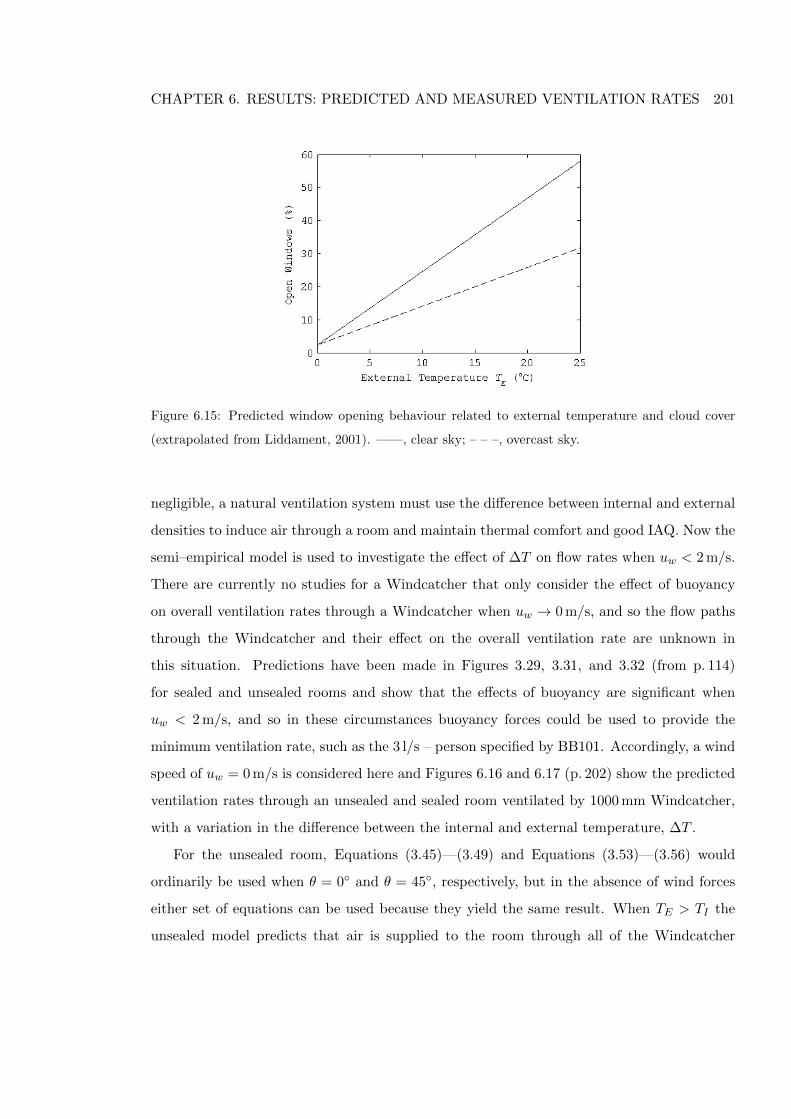
CHAPTER 6. RESULTS: PREDICTED AND MEASURED VENTILATION RATES 201
Figure 6.15: Predicted window opening behaviour related to external temperature and cloud cover
(extrapolated from Liddament, 2001). ——, clear sky; – – –, overcast sky.
negligible, a natural ventilation system must use the difference between internal and external
densities to induce air through a room and maintain thermal comfort and good IAQ. Now the
semi–empirical model is used to investigate the effect of ∆T on flow rates when uw < 2 m/s.
There are currently no studies for a Windcatcher that only consider the effect of buoyancy
on overall ventilation rates through a Windcatcher when uw → 0 m/s, and so the flow paths
through the Windcatcher and their effect on the overall ventilation rate are unknown in
this situation. Predictions have been made in Figures 3.29, 3.31, and 3.32 (from p. 114)
for sealed and unsealed rooms and show that the effects of buoyancy are significant when
uw < 2 m/s, and so in these circumstances buoyancy forces could be used to provide the
minimum ventilation rate, such as the 3 l/s – person specified by BB101. Accordingly, a wind
speed of uw = 0 m/s is considered here and Figures 6.16 and 6.17 (p. 202) show the predicted
ventilation rates through an unsealed and sealed room ventilated by 1000 mm Windcatcher,
with a variation in the difference between the internal and external temperature, ∆T .
For the unsealed room, Equations (3.45)—(3.49) and Equations (3.53)—(3.56) would
ordinarily be used when θ = 0◦ and θ = 45◦, respectively, but in the absence of wind forces
either set of equations can be used because they yield the same result. When TE > TI the
unsealed model predicts that air is supplied to the room through all of the Windcatcher
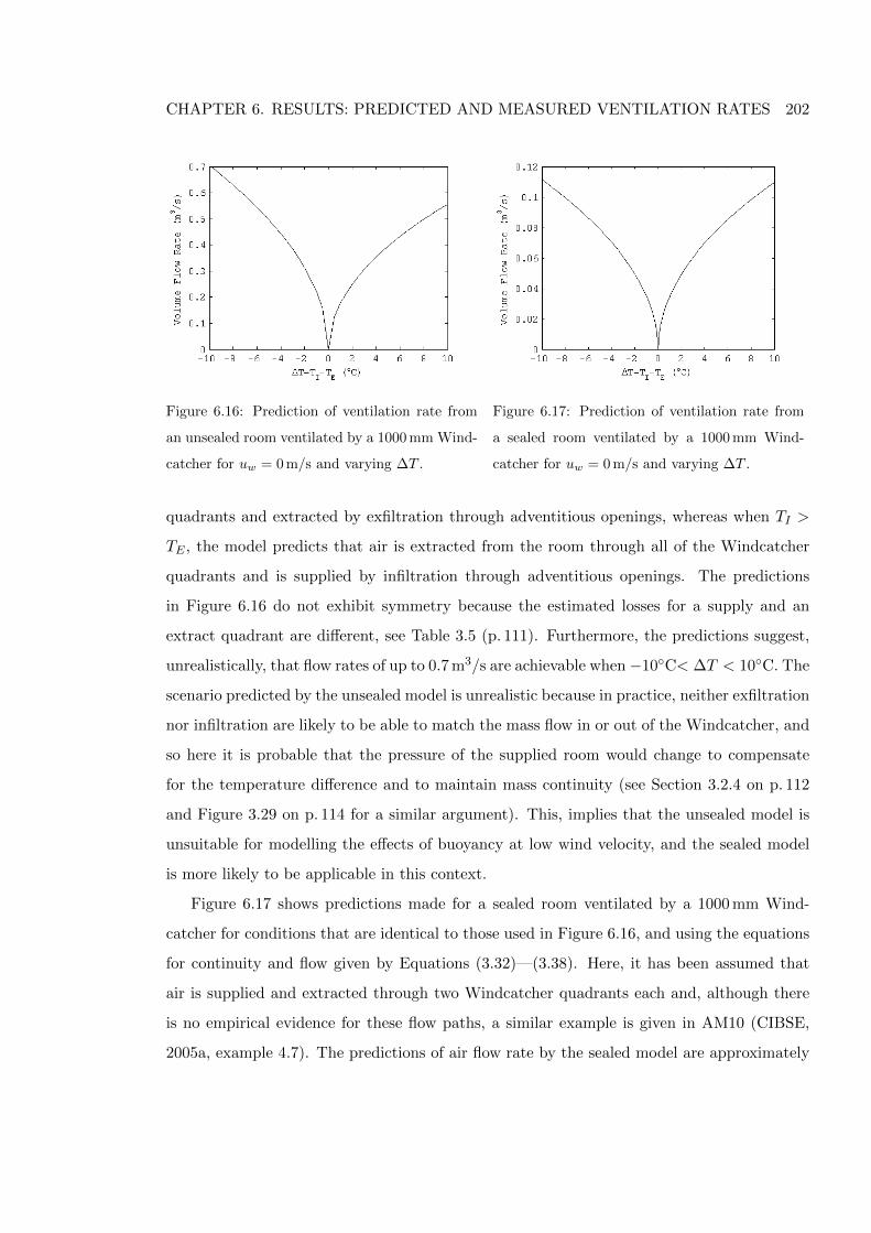
CHAPTER 6. RESULTS: PREDICTED AND MEASURED VENTILATION RATES 202
Figure 6.16: Prediction of ventilation rate from
an unsealed room ventilated by a 1000 mm Wind-
catcher for uw = 0 m/s and varying ∆T .
Figure 6.17: Prediction of ventilation rate from
a sealed room ventilated by a 1000 mm Wind-
catcher for uw = 0 m/s and varying ∆T .
quadrants and extracted by exfiltration through adventitious openings, whereas when TI >
TE , the model predicts that air is extracted from the room through all of the Windcatcher
quadrants and is supplied by infiltration through adventitious openings. The predictions
in Figure 6.16 do not exhibit symmetry because the estimated losses for a supply and an
extract quadrant are different, see Table 3.5 (p. 111). Furthermore, the predictions suggest,
unrealistically, that flow rates of up to 0.7 m3/s are achievable when−10◦C< ∆T < 10◦C. The
scenario predicted by the unsealed model is unrealistic because in practice, neither exfiltration
nor infiltration are likely to be able to match the mass flow in or out of the Windcatcher, and
so here it is probable that the pressure of the supplied room would change to compensate
for the temperature difference and to maintain mass continuity (see Section 3.2.4 on p. 112
and Figure 3.29 on p. 114 for a similar argument). This, implies that the unsealed model is
unsuitable for modelling the effects of buoyancy at low wind velocity, and the sealed model
is more likely to be applicable in this context.
Figure 6.17 shows predictions made for a sealed room ventilated by a 1000 mm Wind-
catcher for conditions that are identical to those used in Figure 6.16, and using the equations
for continuity and flow given by Equations (3.32)—(3.38). Here, it has been assumed that
air is supplied and extracted through two Windcatcher quadrants each and, although there
is no empirical evidence for these flow paths, a similar example is given in AM10 (CIBSE,
2005a, example 4.7). The predictions of air flow rate by the sealed model are approximately
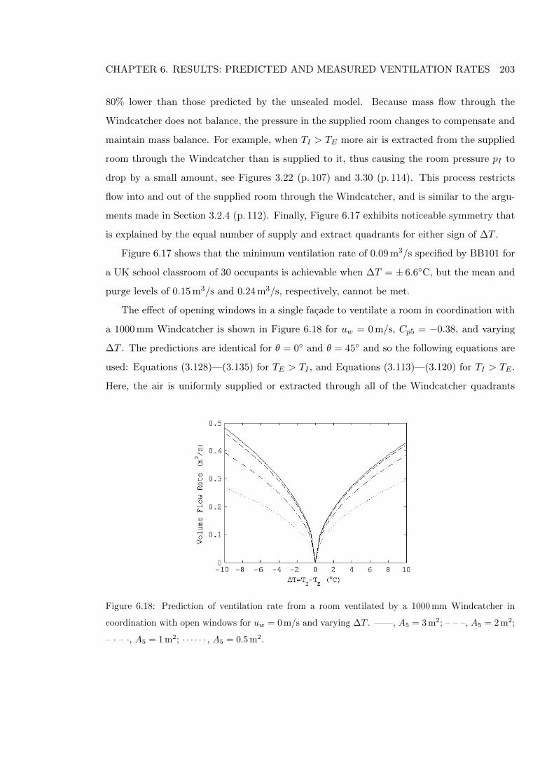
CHAPTER 6. RESULTS: PREDICTED AND MEASURED VENTILATION RATES 203
80% lower than those predicted by the unsealed model. Because mass flow through the
Windcatcher does not balance, the pressure in the supplied room changes to compensate and
maintain mass balance. For example, when TI > TE more air is extracted from the supplied
room through the Windcatcher than is supplied to it, thus causing the room pressure pI to
drop by a small amount, see Figures 3.22 (p. 107) and 3.30 (p. 114). This process restricts
flow into and out of the supplied room through the Windcatcher, and is similar to the argu-
ments made in Section 3.2.4 (p. 112). Finally, Figure 6.17 exhibits noticeable symmetry that
is explained by the equal number of supply and extract quadrants for either sign of ∆T .
Figure 6.17 shows that the minimum ventilation rate of 0.09 m3/s specified by BB101 for
a UK school classroom of 30 occupants is achievable when ∆T = ± 6.6◦C, but the mean and
purge levels of 0.15 m3/s and 0.24 m3/s, respectively, cannot be met.
The effect of opening windows in a single facade to ventilate a room in coordination with
a 1000 mm Windcatcher is shown in Figure 6.18 for uw = 0 m/s, Cp5 = −0.38, and varying
∆T . The predictions are identical for θ = 0◦ and θ = 45◦ and so the following equations are
used: Equations (3.128)—(3.135) for TE > TI , and Equations (3.113)—(3.120) for TI > TE .
Here, the air is uniformly supplied or extracted through all of the Windcatcher quadrants
Figure 6.18: Prediction of ventilation rate from a room ventilated by a 1000 mm Windcatcher in
coordination with open windows for uw = 0 m/s and varying ∆T . ——, A5 = 3 m2; – – –, A5 = 2 m2;
– · – ·, A5 = 1 m2; · · · · · · , A5 = 0.5 m2.
CHAPTER 6. RESULTS: PREDICTED AND MEASURED VENTILATION RATES 204
depending upon the sign of ∆T , and so the flow direction through the Windcatcher quadrants
is the cause of the asymmetry. In Figure 6.18 the area of the open windows A5, is also varied
and shows that as A5 increases the predicted flow rates plateau, thus agreeing with the
findings of Figure 3.33 (p. 120), which also shows that for ever increasing values of A5, the
predicted flow rates reach a peak value. Figure 6.18 suggests that with an opening area of
A5 = 0.5 m3 the background ventilation rate of 0.09 m3/s specified by BB101 for a UK school
classroom of 30 occupants is achievable when −1.5◦C> ∆T > 1◦C, the mean ventilation
rate of 0.15 m3/s is achievable when −3.5◦C> ∆T > 3◦C, and the purge ventilation rate of
0.24 m3/s is achievable when −8◦C> ∆T > 7◦C.
Now, the data presented in Figure 6.15 is recalled that shows approximately 7%—15%
of available openable windows can be expected to be open when the external temperature
is TE = 5◦C; a typical winter temperature. Figure 4.8 (p. 137) shows that the external
temperatures expected in a British winter may cause a temperature difference in excess of
∆T > 10◦ C and so may explain the comparably good measured mean CO2 levels for winter
discussed in Chapter 5 and presented in Figure 5.6 (p. 162). However, Figure 5.4 (p. 160)
shows that Windcatcher volume control dampers were partially open (20%≤ Ad ≤ 100%) for
an average of 17% of occupied hours. Accordingly, the Windcatcher will only have contributed
to the overall ventilation rate for 17% of the time, and ventilation in winter months was likely
to have been provided by open windows and background ventilation for approximately 83% of
occupied hours. This represents a missed opportunity for stack ventilation in winter, because
the predictions given in Figures 6.17 and 6.18 suggest that a Windcatcher system can provide
background ventilatation rates to a classroom autonomously, and mean and purge ventilation
in coordination with open windows.
The methods of sizing a Windcatcher and the predictions of ventilation rates through a
room ventilated by a Windcatcher discussed in this section have all been determined by the
ventilation rates specified by BB101. However, with increasing internal heat gains reported
in UK school classrooms (see Pegg, 2008) the ventilation rate required to dissipate total in-
ternal heat gains may actually be higher than those specified by government requirements
for good IAQ. Therefore, an understanding of the total heat gains in each classroom, and
their effect on the internal air temperatures must be determined. Thermal heat gains arise
from solar heat gains, as well as those from occupants and ICT equipment, but their effect
CHAPTER 6. RESULTS: PREDICTED AND MEASURED VENTILATION RATES 205
can only be estimated by a thermal model, see Lomas & Ji (2009) for example. Here, CIBSE
Guide A Section 5 (CIBSE, 2006a) gives thermal models for winter and summer design calcu-
lations, and more advanced commercial software is also available; for example, the Thermal
Analysis Software (TAS) created by EDSL or Virtual Environment software developed by
Integrated Environmental Solutions (IES). However, it is noted that, when selecting appro-
priate commercial software, it should conform to CIBSE TM33 (CIBSE, 2006b) accreditation
standards.
In winter months it becomes more important to reduce heat lost from a room, and a
primary source of heat loss is that dissipated by the ventilation through a room. Here, the
total heat, H, dissipated from a room by ventilation is approximated by
H = QT ρE cp ∆T (6.1)
where cp is the specific heat capacity of air at constant pressure [cp = 1004 J/kg K (see Fox
& McDonald, 1985, Section 11.1 and Table A.6)]. For a temperature difference of ∆T = 5◦C
where TE = 20◦C, the minimum, mean, and purge ventilation rates specified by BB101 for
a classroom containing 30 occupants are 0.09 m3/s, 0.15 m3/s, and 0.24 m3/s, respectively.
Using Equation (6.1), these ventilation rates correspond to approximately 0.6 kW, 0.9 kW,
and 1.5 kW of dissipated heat, respectively. This is discussed in greater detail, in Chapter 7,
but it is noted here that Equation (6.1) does not account for the thermal characteristics of a
room, its location, orientation, or occupancy patterns, and so it is argued that it is unsuitable
for the calculation of temperature changes in a room when subject to known heat gains.
6.3.1 Design Steps
A series of processes have been tested and discussed in this section that can be employed to
determine the correct CSA of a Windcatcher and openable windows for a particular appli-
cation. These processes are now detailed in chronological order to provide supportive design
steps for a Windcatcher designer. The steps are determined by the assumption that a mean,
purge, and minimum ventilation rate must be provided to a room, in common with the
requirements for BB101.
CHAPTER 6. RESULTS: PREDICTED AND MEASURED VENTILATION RATES 206
Below each test step is a worked example for a hypothetical 2nd floor school classroom of
zI = 3.3 m in height, containing 30 students and staff, and with manually operable windows
located in a single facade. It is ventilated by an unlined Windcatcher of duct length 1m,
whose faces are normal to the cardinal points. The school is located in the south west of
England, is zE =10 m high, has topography defined as urban, is surrounded by obstructions
equal to the height of the building, and has an aspect ratio of 2:1 with the windows located
in the longer side. The ventilation rates and IAQ in the classroom must conform to those
stated in BB101 and so a mean ventilation rate of 5 l/s – person, a purge ventilation rate of
8 l/s – person, and a minimum ventilation rate of 3 l/s – person must be supplied.
6.3.1.1 Providing a Mean Ventilation Rate
Firstly, the CSA of an autonomous Windcatcher to provide the required mean ventilation
rate to a room is calculated.
1. Select required mean ventilation rate:
(a) Using government ventilation guidelines, such as BB101 (DfES, 2006) or Building
Regulations, Part F (ODPM, 2006).
(b) To dissipate internal heat gains. An appropriate ventilation rate should be deter-
mined using a thermal model.
BB101 recommends a ventilation rate of 5 l/s – person, so for a room containing 30 occupants,
the total required ventilation rate is 150 l/s (0.15 m3/s). For the purposes of this example,
the mean ventilation rate required to dissipate total heat gains in a room is supplied by
the contractor and is calculated to be 0.14 m3/s. Therefore, the greater ventilation rate of
0.15 m3/s is used as the design ventilation rate.
2. Use aerial photographs or other relevant sources to determine the local topography and
relevant topographical constants k and a, see those given by Orme & Leksmono (2002,
Table 2) for example.
For an urban location Orme & Leksmono (2002) give k = 0.35 m−a and a = 0.25.
CHAPTER 6. RESULTS: PREDICTED AND MEASURED VENTILATION RATES 207
3. Select CIBSE TRY weather data (CIBSE 2005) for the relevant region and scale the
wind speed data appropriately to determine the wind speed at roof level using Equation
(3.18) and the topographical constants determined at Stage 2.
Figure 4.11 presents wind speeds for the south west of England and the mean wind speed is
shown to be 5.91 m/s. The school building is zE = 10 m high, and so using Equation (3.18)
uw = u10kzEa
5.91× 0.35× 100.25 = 3.68 m/s
the mean wind speed for the south east of England of u10 = 5.91 m/s equates to uw = 3.68 m/s
at roof level. CIBSE TRY data is given hourly, and all wind speeds are similarly scaled.
4. Determine the orientation of the Windcatcher faces relative to the points of a compass.
The Windcatcher faces are oriented to the cardinal points so that they face 0◦, 90◦, 180◦, and
270◦. Therefore, when the wind angle is at an angle of ± 22.5◦C from the cardinal points the
wind is considered to be normal to a single Windcatcher quadrant so that θ = 0◦. Otherwise
the wind is considered to be incident to two Windcatcher quadrants so that θ = 45◦.
5. Select the initial CSA of the Windcatcher using the simplified semi–empirical model
given by Equation (3.148).
Equation (3.148) is rearranged to give a simple relationship between the total cross sectional
area of a Windcatcher, the flow rate out of it, and the wind speed.
AT =QT
0.1251uw(6.2)
Application of the design flow rate and the scaled mean wind speed to Equation 6.2 gives
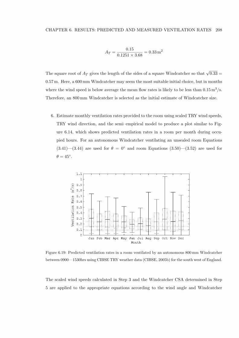
CHAPTER 6. RESULTS: PREDICTED AND MEASURED VENTILATION RATES 208
AT =0.15
0.1251× 3.68= 0.33 m2
The square root of AT gives the length of the sides of a square Windcatcher so that√
0.33 =
0.57 m. Here, a 600 mm Windcatcher may seem the most suitable initial choice, but in months
where the wind speed is below average the mean flow rates is likely to be less than 0.15 m3/s.
Therefore, an 800 mm Windcatcher is selected as the initial estimate of Windcatcher size.
6. Estimate monthly ventilation rates provided to the room using scaled TRY wind speeds,
TRY wind direction, and the semi–empirical model to produce a plot similar to Fig-
ure 6.14, which shows predicted ventilation rates in a room per month during occu-
pied hours. For an autonomous Windcatcher ventilating an unsealed room Equations
(3.41)—(3.44) are used for θ = 0◦ and room Equations (3.50)—(3.52) are used for
θ = 45◦.
Figure 6.19: Predicted ventilation rates in a room ventilated by an autonomous 800 mm Windcatcher
between 0900—1530hrs using CIBSE TRY weather data (CIBSE, 2005b) for the south west of England.
The scaled wind speeds calculated in Step 3 and the Windcatcher CSA determined in Step
5 are applied to the appropriate equations according to the wind angle and Windcatcher
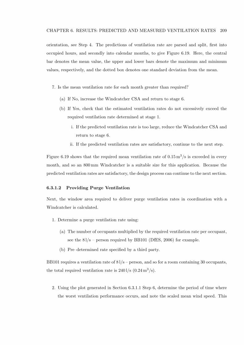
CHAPTER 6. RESULTS: PREDICTED AND MEASURED VENTILATION RATES 209
orientation, see Step 4. The predictions of ventilation rate are parsed and split, first into
occupied hours, and secondly into calendar months, to give Figure 6.19. Here, the central
bar denotes the mean value, the upper and lower bars denote the maximum and minimum
values, respectively, and the dotted box denotes one standard deviation from the mean.
7. Is the mean ventilation rate for each month greater than required?
(a) If No, increase the Windcatcher CSA and return to stage 6.
(b) If Yes, check that the estimated ventilation rates do not excessively exceed the
required ventilation rate determined at stage 1.
i. If the predicted ventilation rate is too large, reduce the Windcatcher CSA and
return to stage 6.
ii. If the predicted ventilation rates are satisfactory, continue to the next step.
Figure 6.19 shows that the required mean ventilation rate of 0.15 m3/s is exceeded in every
month, and so an 800 mm Windcatcher is a suitable size for this application. Because the
predicted ventilation rates are satisfactory, the design process can continue to the next section.
6.3.1.2 Providing Purge Ventilation
Next, the window area required to deliver purge ventilation rates in coordination with a
Windcatcher is calculated.
1. Determine a purge ventilation rate using:
(a) The number of occupants multiplied by the required ventilation rate per occupant,
see the 8 l/s – person required by BB101 (DfES, 2006) for example.
(b) Pre–determined rate specified by a third party.
BB101 requires a ventilation rate of 8 l/s – person, and so for a room containing 30 occupants,
the total required ventilation rate is 240 l/s (0.24 m3/s).
2. Using the plot generated in Section 6.3.1.1 Step 6, determine the period of time where
the worst ventilation performance occurs, and note the scaled mean wind speed. This
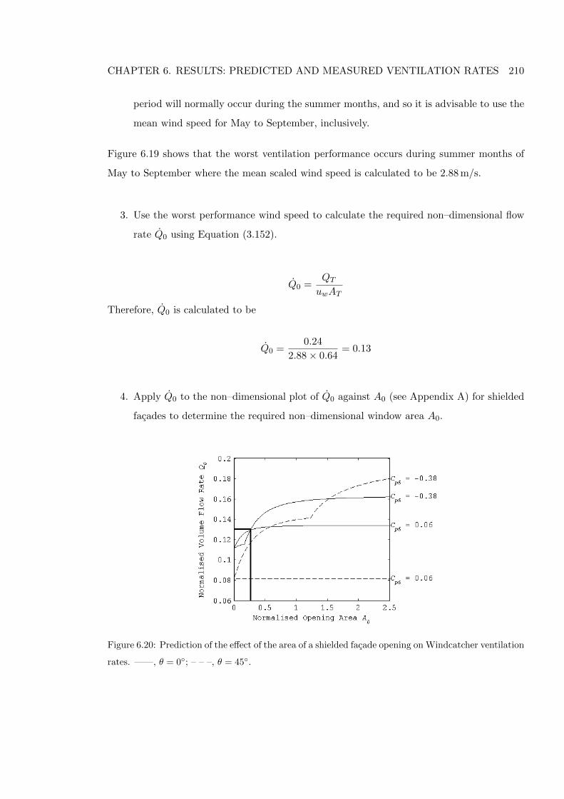
CHAPTER 6. RESULTS: PREDICTED AND MEASURED VENTILATION RATES 210
period will normally occur during the summer months, and so it is advisable to use the
mean wind speed for May to September, inclusively.
Figure 6.19 shows that the worst ventilation performance occurs during summer months of
May to September where the mean scaled wind speed is calculated to be 2.88 m/s.
3. Use the worst performance wind speed to calculate the required non–dimensional flow
rate Q0 using Equation (3.152).
Q0 =QT
uwAT
Therefore, Q0 is calculated to be
Q0 =0.24
2.88× 0.64= 0.13
4. Apply Q0 to the non–dimensional plot of Q0 against A0 (see Appendix A) for shielded
facades to determine the required non–dimensional window area A0.
Figure 6.20: Prediction of the effect of the area of a shielded facade opening on Windcatcher ventilation
rates. ——, θ = 0◦; – – –, θ = 45◦.
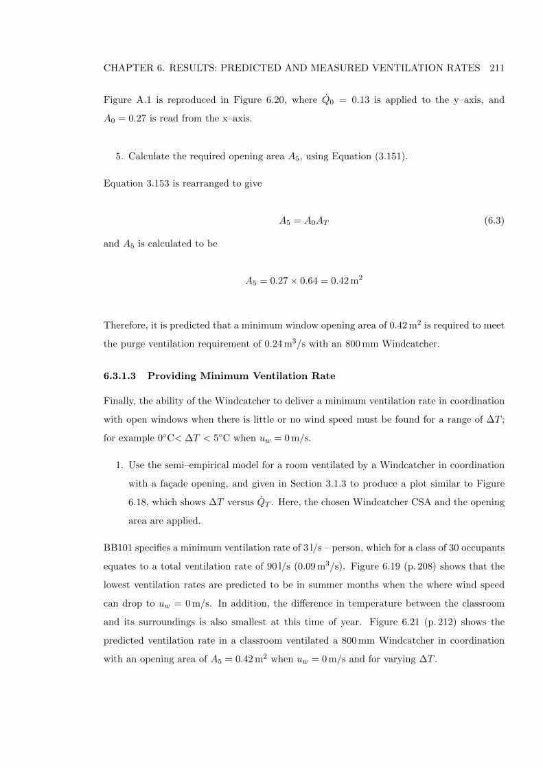
CHAPTER 6. RESULTS: PREDICTED AND MEASURED VENTILATION RATES 211
Figure A.1 is reproduced in Figure 6.20, where Q0 = 0.13 is applied to the y–axis, and
A0 = 0.27 is read from the x–axis.
5. Calculate the required opening area A5, using Equation (3.151).
Equation 3.153 is rearranged to give
A5 = A0AT (6.3)
and A5 is calculated to be
A5 = 0.27× 0.64 = 0.42 m2
Therefore, it is predicted that a minimum window opening area of 0.42 m2 is required to meet
the purge ventilation requirement of 0.24 m3/s with an 800 mm Windcatcher.
6.3.1.3 Providing Minimum Ventilation Rate
Finally, the ability of the Windcatcher to deliver a minimum ventilation rate in coordination
with open windows when there is little or no wind speed must be found for a range of ∆T ;
for example 0◦C< ∆T < 5◦C when uw = 0 m/s.
1. Use the semi–empirical model for a room ventilated by a Windcatcher in coordination
with a facade opening, and given in Section 3.1.3 to produce a plot similar to Figure
6.18, which shows ∆T versus QT . Here, the chosen Windcatcher CSA and the opening
area are applied.
BB101 specifies a minimum ventilation rate of 3 l/s – person, which for a class of 30 occupants
equates to a total ventilation rate of 90 l/s (0.09 m3/s). Figure 6.19 (p. 208) shows that the
lowest ventilation rates are predicted to be in summer months when the where wind speed
can drop to uw = 0 m/s. In addition, the difference in temperature between the classroom
and its surroundings is also smallest at this time of year. Figure 6.21 (p. 212) shows the
predicted ventilation rate in a classroom ventilated a 800 mm Windcatcher in coordination
with an opening area of A5 = 0.42 m2 when uw = 0 m/s and for varying ∆T .
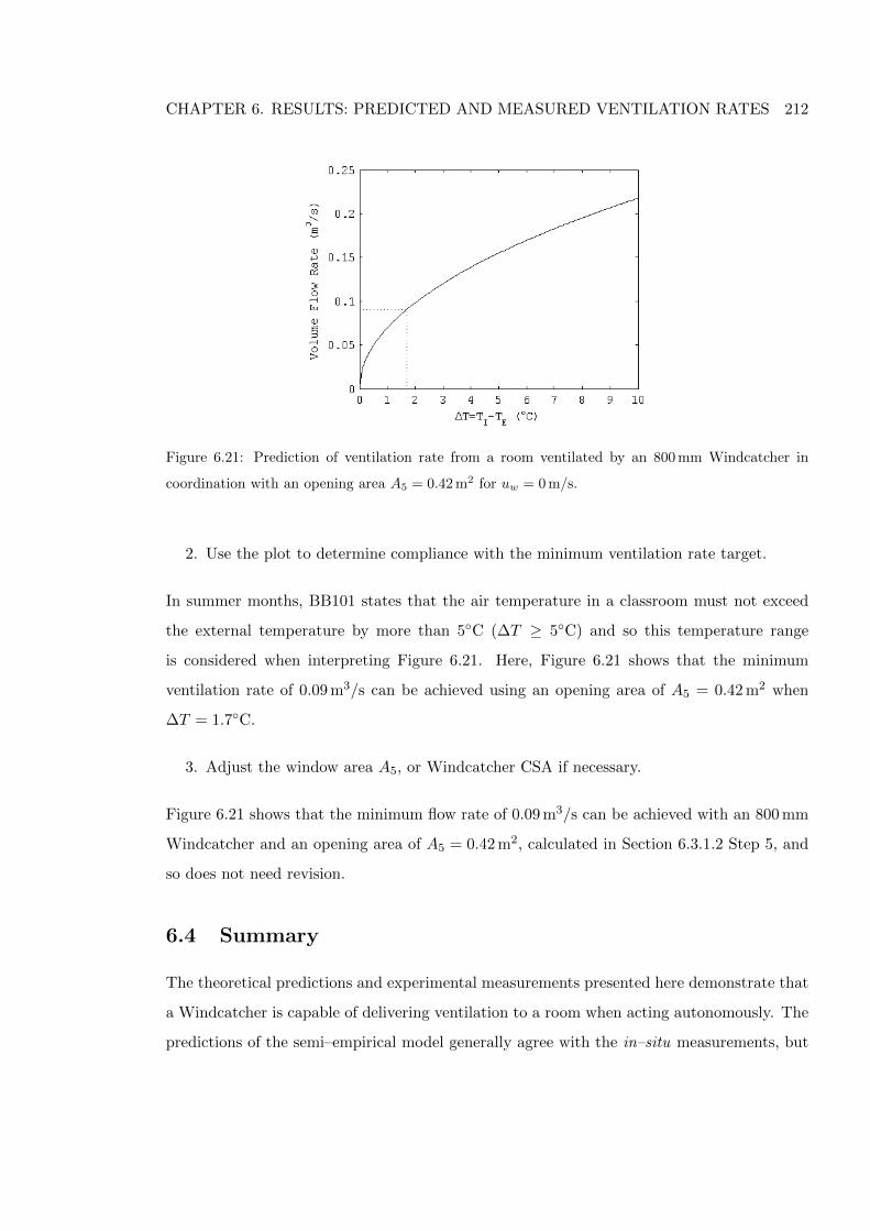
CHAPTER 6. RESULTS: PREDICTED AND MEASURED VENTILATION RATES 212
Figure 6.21: Prediction of ventilation rate from a room ventilated by an 800 mm Windcatcher in
coordination with an opening area A5 = 0.42 m2 for uw = 0 m/s.
2. Use the plot to determine compliance with the minimum ventilation rate target.
In summer months, BB101 states that the air temperature in a classroom must not exceed
the external temperature by more than 5◦C (∆T ≥ 5◦C) and so this temperature range
is considered when interpreting Figure 6.21. Here, Figure 6.21 shows that the minimum
ventilation rate of 0.09 m3/s can be achieved using an opening area of A5 = 0.42 m2 when
∆T = 1.7◦C.
3. Adjust the window area A5, or Windcatcher CSA if necessary.
Figure 6.21 shows that the minimum flow rate of 0.09 m3/s can be achieved with an 800 mm
Windcatcher and an opening area of A5 = 0.42 m2, calculated in Section 6.3.1.2 Step 5, and
so does not need revision.
6.4 Summary
The theoretical predictions and experimental measurements presented here demonstrate that
a Windcatcher is capable of delivering ventilation to a room when acting autonomously. The
predictions of the semi–empirical model generally agree with the in–situ measurements, but
CHAPTER 6. RESULTS: PREDICTED AND MEASURED VENTILATION RATES 213
ventilation rates through a room ventilated by an autonomous Windcatcher are sometimes
over–predicted and significant scatter in the experimental data is observed. The relatively
poor performance of Windcatchers with long duct sections was not predicted and further
investigation of such devices is required, see Chapter 7 for a discussion. Furthermore, the
measured volume flow rates for a Windcatcher with closed windows do not exceed 0.23 m3/s,
and appear to plateau when uw ≥ 2 m/s. This too is not predicted by the model and its cause
is unclear. Both the theoretical and experimental analysis of the Windcatcher demonstrate
that Windcatcher performance can be significantly improved by the addition of open windows
to a room. This aspect is likely to help rooms ventilated by a Windcatcher to meet ventilation
standards for buildings, such as BB101 in the UK (DfES, 2006). In these circumstances the
careful selection of Cp5 for a building is important for the accuracy of the semi–empirical
predictions.
Typical wind conditions for the south–east of England were applied to the semi–empirical
model using the CIBSE TRY database to predict the ventilation performance of a room
ventilated by a Windcatcher every month, and was shown to be a useful design tool. It also
identified situations where the wind speed was negligible, and here the Windcatcher system
must rely on buoyancy forces to generate ventilation through a room. When the semi–
empirical model was used to investigate this situation, the unsealed model is found to be
unsuitable for situations where uw < 2 m/s and |∆T | > 0◦C. The sealed model may be used
to estimate ventilation rates under these circumstances and although the predictions seem
plausible, they remain uncorroborated by empirical measurement. The predictions suggest
that an autonomous Windcatcher is capable of providing minimum ventilation rates specified
by BB101 for a class of 30 occupants, and a Windcatcher in coordination with open windows
can provide minimum, mean, and purge ventilation rates.
Finally, the investigation of the capabilities of the semi–empirical model produced a series
of steps that a designer may use to correctly size a Windcatcher for a particular application.
The ramifications of these findings are discussed in Chapter 7.
CHAPTER 7. DISCUSSION OF RESULTS 214
Chapter 7
Discussion of results
This chapter discusses issues raised during the course of this research, particularly methods
of providing optimum thermal comfort and good IAQ to occupants, efficient flow paths for
effective ventilation and energy conservation, improvements to Windcatcher system design
and control, opportunities for the implementation of Windcatcher systems in building types
other than schools, and immediate applications of this work. Finally, conclusions are proffered
in Chapter 8.
7.1 Providing Thermal Comfort and Air Quality
It has been shown that a Windcatcher can provide a supply of fresh air to a room both
autonomously and in coordination with open windows. External air is delivered to a room to
maintain the quality of the indoor air and the thermal comfort of occupants. Indoor air quality
is indicated by the concentration of carbon dioxide in a room, and in the classrooms measured
for this study, mean CO2 concentrations during occupied hours are shown in Chapter 5 to be
682 ppm in summer months and 1350 ppm in winter months. It is clear that the air quality
and ventilation is better in these classrooms in summer months than in winter months,
although the exact difference cannot be quantified by these values. The CO2 concentration
was found in Chapters 5 and 6 to be a function of the position of the Windcatcher dampers
and the presence of open windows. The number of open windows is related to the external air
temperature (see Figure 6.18, p. 203), and the position of the damper is determined by the
internal air temperature. However, the ability of the dampers to regulate the rate of air flow
CHAPTER 7. DISCUSSION OF RESULTS 215
through the Windcatcher system is not yet quantified, despite a study by Hughes & Ghani
(2009) who used CFD to investigate the effect that dampers have on overall flow rates through
a Windcatcher. Their results confusingly suggest that a flow rate through the Windcatcher
can be achieved when the dampers are fully closed. Furthermore, they model contra–rotating
dampers, whereas the Monodraught Windcatcher system uses counter–rotating dampers.
Hughes and Ghani also present several diagrams that indicate flow paths (see Figures 10
and 13, Hughes & Ghani, 2008) that clearly shows short circuiting in the space between the
bottom of the duct partition and fully open dampers, but there is no indication of how this
phenomena changes when the damper angle is reduced. Here, the quantity of short circuiting
is expected to escalate with an increase in the space between the bottom of the duct partition
and the dampers.
Currently, the control system increases the damper angle linearly at a rate of 20% per ◦C
above the initial set point temperature, which corresponds to a non–linear increase in the
free area of the damper. If it is assumed that the total flow rate through the damper is
proportional to their free area (QT ∝ Ad), where Ad is the percentage free area of the volume
control dampers, then the control system should be amended so that the free area of the
dampers is increased linearly with each temperature set point, thus increasing the supply
of air when the damper ange γ, is small (see Section 4.3, p. 143). The relationship between
Ad and γ is described by Equation (4.3), which assumes that the dampers are flat plates of
negligible thickness. Equation (4.3) is now rearranged to give
γ = cos−1(1−Ad) (7.1)
where, for a required damper free area of 20% (Ad = 0.2), the associated angle should be
γ = 37◦ rather than the value of γ = 18◦ that is currently used. This simple change will allow
more air to enter a room through the Windcatcher system at low damper angles, which is
particularly important to ensure good IAQ in winter months when the temperature set point
is higher than in summer months.
It may be argued that providing ventilation in the winter acts in opposition to the imple-
mentation of space heating. In Section 6.3 (p. 195) it was shown that for a class of 30 occu-
CHAPTER 7. DISCUSSION OF RESULTS 216
pants the minimum, mean, and purge ventilation rates of 0.09 m3/s, 0.15 m3/s, and 0.24 m3/s,
respectively, required by BB101 (DfES, 2006) will dissipate approximately 0.6 kW, 0.9 kW,
and 1.5 kW of heat if ∆T = 5◦C. However, if occupancy levels falls below 30 then the required
volume flow rate reduces, and so if the BB101 requirements are to be met while minimising
heat losses by ventilation, a more intelligent control system is required that can implicitly
determine the number of occupants in the room and calculate the volume flow rate required
to deliver the per capita ventilation rate specified by BB101.
7.1.1 Demand Control Ventilation
Heiselberg (2004) suggests that increases in heating costs incurred from winter ventilation can
be mitigated by demand controlled ventilation, thermal mass, embedded ducts, and/or heat
recovery. Heat recovery systems are likely to be unfeasible for a Windcatcher because they
would increase the pressure drop across the Windcatcher quadrants adversely affecting flow
rates, and are also likely to be impractical because Windcatcher quadrants frequently switch
from supplying to extracting air with small changes of wind incidence. Embedded ducts and
thermal mass are architectural considerations and so are not considered here, although it is
acknowledged that they may be useful. However, it is possible to control a Windcatcher using
a demand control strategy, which has been shown to be effective by Haghighat & Donnini
(1993) who controlled a mechanical ventilation system using a CO2 based control strategy
that did not worsen IAQ or thermal comfort and provided a 12% energy saving. Mysen
et al. (2005) show a 28% reduction in the energy consumed by a mechanical ventilations
system measured in 157 classroom from 81 schools when controlled by CO2 based demand
control ventilation. Applying a demand control strategy to a classroom would minimise
heat losses; for example, the heat lost from a room with varying flow rate per occupant is
given in Figure 7.1 (p. 217), and shows for a ventilation rate of 5 l/s – person (the mean rate
required by BB101) and ∆T = 10◦C, the energy lost through ventilation is approximately
62 W – person. This loss could be recouped by incidental heat gains from ICT equipment
and the metabolic heat of occupants. In fact, BB87 (DfEE, 2003) suggests that “pupils in a
classroom will compensate for all fabric losses and a major part of ventilation heat losses.”
Heat gains from a child are not given in CIBSE environmental guidelines, but a single male
or female adult occupant, seated and doing light work is estimated to generate a total heat
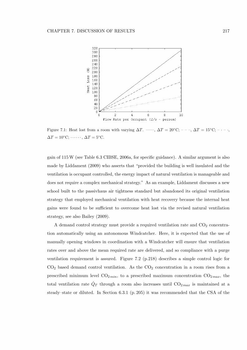
CHAPTER 7. DISCUSSION OF RESULTS 217
Figure 7.1: Heat lost from a room with varying ∆T . ——, ∆T = 20◦C; – – –, ∆T = 15◦C; – · – ·,
∆T = 10◦C; · · · · · · , ∆T = 5◦C.
gain of 115 W (see Table 6.3 CIBSE, 2006a, for specific guidance). A similar argument is also
made by Liddament (2009) who asserts that “provided the building is well insulated and the
ventilation is occupant controlled, the energy impact of natural ventilation is manageable and
does not require a complex mechanical strategy.” As an example, Liddament discusses a new
school built to the passivhaus air tightness standard but abandoned its original ventilation
strategy that employed mechanical ventilation with heat recovery because the internal heat
gains were found to be sufficient to overcome heat lost via the revised natural ventilation
strategy, see also Bailey (2009).
A demand control strategy must provide a required ventilation rate and CO2 concentra-
tion automatically using an autonomous Windcatcher. Here, it is expected that the use of
manually opening windows in coordination with a Windcatcher will ensure that ventilation
rates over and above the mean required rate are delivered, and so compliance with a purge
ventilation requirement is assured. Figure 7.2 (p.218) describes a simple control logic for
CO2 based demand control ventilation. As the CO2 concentration in a room rises from a
prescribed minimum level CO2min, to a prescribed maximum concentration CO2max, the
total ventilation rate QT through a room also increases until CO2max is maintained at a
steady–state or diluted. In Section 6.3.1 (p. 205) it was recommended that the CSA of the
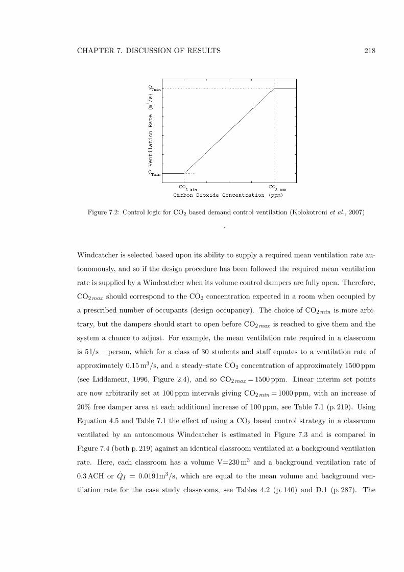
CHAPTER 7. DISCUSSION OF RESULTS 218
Figure 7.2: Control logic for CO2 based demand control ventilation (Kolokotroni et al., 2007)
.
Windcatcher is selected based upon its ability to supply a required mean ventilation rate au-
tonomously, and so if the design procedure has been followed the required mean ventilation
rate is supplied by a Windcatcher when its volume control dampers are fully open. Therefore,
CO2max should correspond to the CO2 concentration expected in a room when occupied by
a prescribed number of occupants (design occupancy). The choice of CO2min is more arbi-
trary, but the dampers should start to open before CO2max is reached to give them and the
system a chance to adjust. For example, the mean ventilation rate required in a classroom
is 5 l/s – person, which for a class of 30 students and staff equates to a ventilation rate of
approximately 0.15 m3/s, and a steady–state CO2 concentration of approximately 1500 ppm
(see Liddament, 1996, Figure 2.4), and so CO2max = 1500 ppm. Linear interim set points
are now arbitrarily set at 100 ppm intervals giving CO2min = 1000 ppm, with an increase of
20% free damper area at each additional increase of 100 ppm, see Table 7.1 (p. 219). Using
Equation 4.5 and Table 7.1 the effect of using a CO2 based control strategy in a classroom
ventilated by an autonomous Windcatcher is estimated in Figure 7.3 and is compared in
Figure 7.4 (both p. 219) against an identical classroom ventilated at a background ventilation
rate. Here, each classroom has a volume V=230 m3 and a background ventilation rate of
0.3 ACH or QI = 0.0191m3/s, which are equal to the mean volume and background ven-
tilation rate for the case study classrooms, see Tables 4.2 (p. 140) and D.1 (p. 287). The
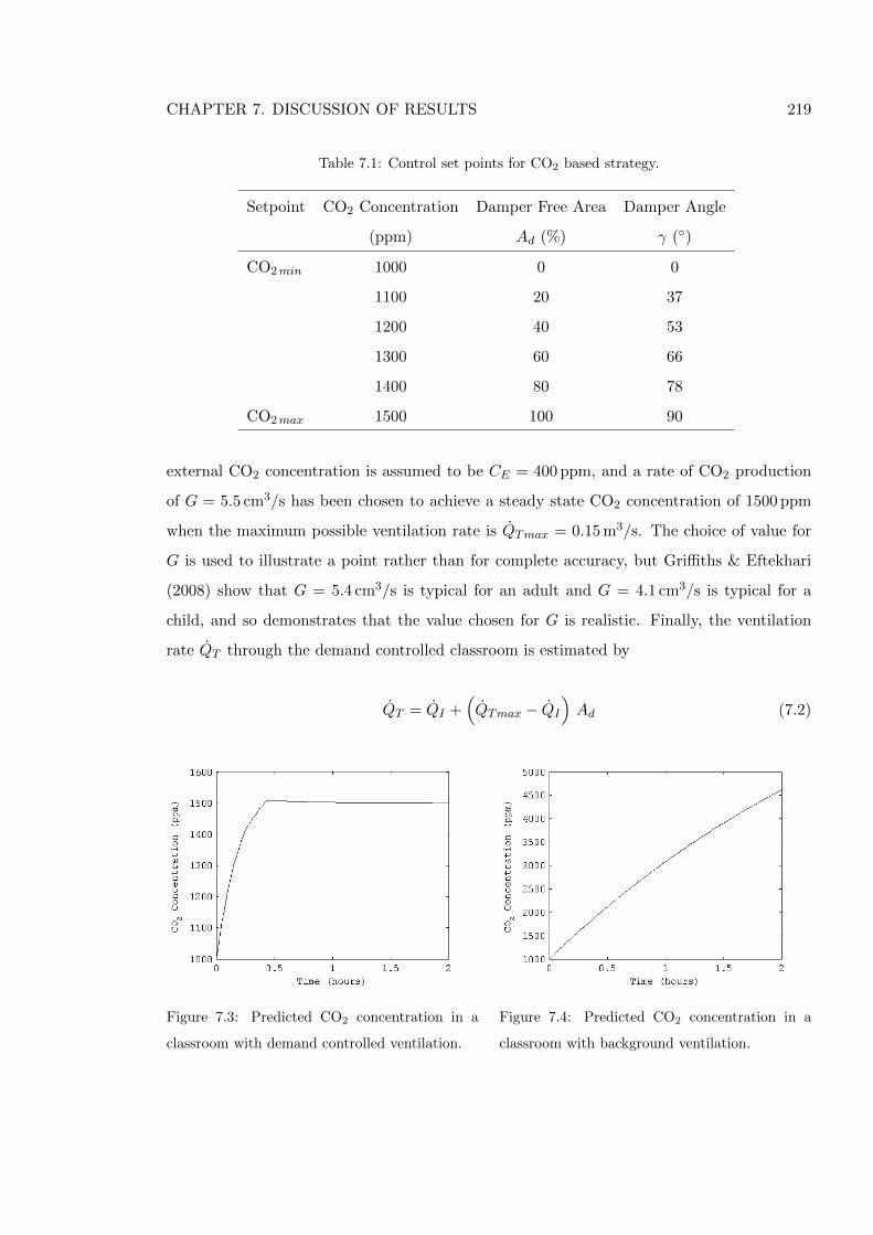
CHAPTER 7. DISCUSSION OF RESULTS 219
Table 7.1: Control set points for CO2 based strategy.
Setpoint CO2 Concentration Damper Free Area Damper Angle
(ppm) Ad (%) γ (◦)
CO2min 1000 0 0
1100 20 37
1200 40 53
1300 60 66
1400 80 78
CO2max 1500 100 90
external CO2 concentration is assumed to be CE = 400 ppm, and a rate of CO2 production
of G = 5.5 cm3/s has been chosen to achieve a steady state CO2 concentration of 1500 ppm
when the maximum possible ventilation rate is QTmax = 0.15 m3/s. The choice of value for
G is used to illustrate a point rather than for complete accuracy, but Griffiths & Eftekhari
(2008) show that G = 5.4 cm3/s is typical for an adult and G = 4.1 cm3/s is typical for a
child, and so demonstrates that the value chosen for G is realistic. Finally, the ventilation
rate QT through the demand controlled classroom is estimated by
QT = QI +(QTmax − QI
)Ad (7.2)
Figure 7.3: Predicted CO2 concentration in a
classroom with demand controlled ventilation.
Figure 7.4: Predicted CO2 concentration in a
classroom with background ventilation.
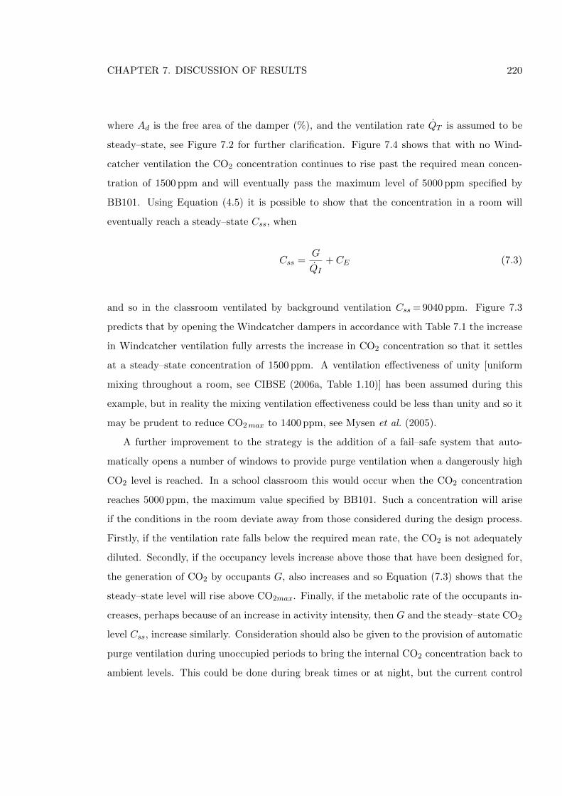
CHAPTER 7. DISCUSSION OF RESULTS 220
where Ad is the free area of the damper (%), and the ventilation rate QT is assumed to be
steady–state, see Figure 7.2 for further clarification. Figure 7.4 shows that with no Wind-
catcher ventilation the CO2 concentration continues to rise past the required mean concen-
tration of 1500 ppm and will eventually pass the maximum level of 5000 ppm specified by
BB101. Using Equation (4.5) it is possible to show that the concentration in a room will
eventually reach a steady–state Css, when
Css =G
QI
+ CE (7.3)
and so in the classroom ventilated by background ventilation Css = 9040 ppm. Figure 7.3
predicts that by opening the Windcatcher dampers in accordance with Table 7.1 the increase
in Windcatcher ventilation fully arrests the increase in CO2 concentration so that it settles
at a steady–state concentration of 1500 ppm. A ventilation effectiveness of unity [uniform
mixing throughout a room, see CIBSE (2006a, Table 1.10)] has been assumed during this
example, but in reality the mixing ventilation effectiveness could be less than unity and so it
may be prudent to reduce CO2max to 1400 ppm, see Mysen et al. (2005).
A further improvement to the strategy is the addition of a fail–safe system that auto-
matically opens a number of windows to provide purge ventilation when a dangerously high
CO2 level is reached. In a school classroom this would occur when the CO2 concentration
reaches 5000 ppm, the maximum value specified by BB101. Such a concentration will arise
if the conditions in the room deviate away from those considered during the design process.
Firstly, if the ventilation rate falls below the required mean rate, the CO2 is not adequately
diluted. Secondly, if the occupancy levels increase above those that have been designed for,
the generation of CO2 by occupants G, also increases and so Equation (7.3) shows that the
steady–state level will rise above CO2max. Finally, if the metabolic rate of the occupants in-
creases, perhaps because of an increase in activity intensity, then G and the steady–state CO2
level Css, increase similarly. Consideration should also be given to the provision of automatic
purge ventilation during unoccupied periods to bring the internal CO2 concentration back to
ambient levels. This could be done during break times or at night, but the current control
CHAPTER 7. DISCUSSION OF RESULTS 221
system only allows an occupant to either activate the manual override that fully opens the
Windcatcher flow control dampers or to open a window. Therefore, automatically opening
facade windows in coordination with the Windcatcher dampers will deliver purge ventilation
without occupant input.
A cheaper alternative to demand control ventilation is to engage the occupants; for ex-
ample, an intervention study in The Netherlands (Geelen et al., 2008) shows that occupant
engagement produced a limited improvement in the IAQ of 81 primary school classrooms
using a teaching package and/or a CO2 indication device. However, an educational strategy
is only likely to have limited application, because it faces challenges from staff turnover and
the high levels of class rotation by teachers of secondary (high) school children. Education is
certainly required to inform occupants on the Windcatcher system’s capability and how the
override system functions, and this could have an important part to play in the management
of occupant expectations. Although it may be reasoned that the teachers and students who
occupy a school classroom should concentrate on the processes of learning rather than man-
aging their ventilation system, giving them control over their environment is very important,
see Brager & De Dear (1998). In fact, Mavrogianni (2007) suggests that the efficient control
of a natural ventilation system translates into an increase in operability and is the most im-
portant way to enhance thermal comfort in school environments. The CO2 indication device
used by Geelen et al. (2008) is a traffic light warning system that displays a green, amber,
or red light emitting diode to indicate optimal, moderate, or poor IAQ. While it could be
argued that warning occupants of poor IAQ may have commercial implications for a product
such as a Windcatcher, recognition of the limitations of natural ventilation suggests that
this is a sensible option which would guide occupants to open windows in coordination with
the Windcatcher. In a school classroom the traffic light warning system could be used to
indicate amber when the internal CO2 concentration exceeds 1500 ppm and red when it ex-
ceeds 5000 ppm. Alternatively, in an office environment the warning system could be indicate
air quality categories given by BS EN 15251 (BSI, 2007). If the office was designed to meet
category II conditions (normal level of expectation, 7 l/s – person) the warning device could
indicate amber for category III conditions (acceptable level of expectation, 4 l/s – person)
and red for category IV conditions (acceptable at limited times of the year, <4 l/s – person).
Finally, it should be noted that if an occupant activates the Windcatcher override, the
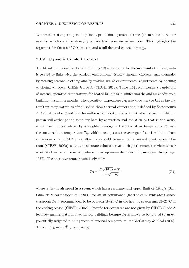
CHAPTER 7. DISCUSSION OF RESULTS 222
Windcatcher dampers open fully for a pre–defined period of time (15 minutes in winter
months) which could be draughty and/or lead to excessive heat loss. This highlights the
argument for the use of CO2 sensors and a full demand control strategy.
7.1.2 Dynamic Comfort Control
The literature review (see Section 2.1.1, p. 29) shows that the thermal comfort of occupants
is related to links with the outdoor environment visually through windows, and thermally
by wearing seasonal clothing and by making use of environmental adjustments by opening
or closing windows. CIBSE Guide A (CIBSE, 2006a, Table 1.5) recommends a bandwidth
of internal operative temperatures for heated buildings in winter months and air conditioned
buildings in summer months. The operative temperature TO, also known in the UK as the dry
resultant temperature, is often used to show thermal comfort and is defined by Santamouris
& Asimakopoulos (1996) as the uniform temperature of a hypothetical space at which a
person will exchange the same dry heat by convection and radiation as that in the actual
environment. It calculated by a weighted average of the internal air temperature TI , and
the mean radiant temperature TR, which encompasses the average effect of radiation from
surfaces in a room (McMullan, 2002). TO should be measured at several points around the
room (CIBSE, 2006a), so that an accurate value is derived, using a thermometer whose sensor
is situated inside a blackened globe with an optimum diameter of 40 mm (see Humphreys,
1977). The operative temperature is given by
TO =TI√
10uI + TR1 +√
10uI(7.4)
where uI is the air speed in a room, which has a recommended upper limit of 0.8 m/s (San-
tamouris & Asimakopoulos, 1996). For an air conditioned (mechanically ventilated) school
classroom TO is recommended to be between 19–21◦C in the heating season and 21–23◦C in
the cooling season (CIBSE, 2006a). Specific temperatures are not given by CIBSE Guide A
for free–running, naturally ventilated, buildings because TO is known to be related to an ex-
ponentially weighted running mean of external temperature, see McCartney & Nicol (2002).
The running mean Trm, is given by
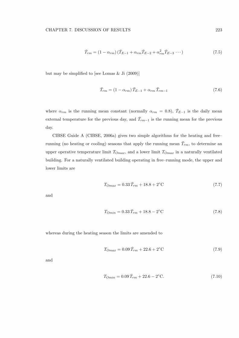
CHAPTER 7. DISCUSSION OF RESULTS 223
Trm = (1− αrm) (TE−1 + αrmTE−2 + α2rmTE−3 · · · ) (7.5)
but may be simplified to [see Lomas & Ji (2009)]
Trm = (1− αrm) TE−1 + αrm Trm−1 (7.6)
where αrm is the running mean constant (normally αrm = 0.8), TE−1 is the daily mean
external temperature for the previous day, and Trm−1 is the running mean for the previous
day.
CIBSE Guide A (CIBSE, 2006a) gives two simple algorithms for the heating and free–
running (no heating or cooling) seasons that apply the running mean Trm, to determine an
upper operative temperature limit TOmax, and a lower limit TOmax in a naturally ventilated
building. For a naturally ventilated building operating in free–running mode, the upper and
lower limits are
TOmax = 0.33 Trm + 18.8 + 2◦C (7.7)
and
TOmin = 0.33 Trm + 18.8− 2◦C (7.8)
whereas during the heating season the limits are amended to
TOmax = 0.09 Trm + 22.6 + 2◦C (7.9)
and
TOmin = 0.09 Trm + 22.6− 2◦C. (7.10)
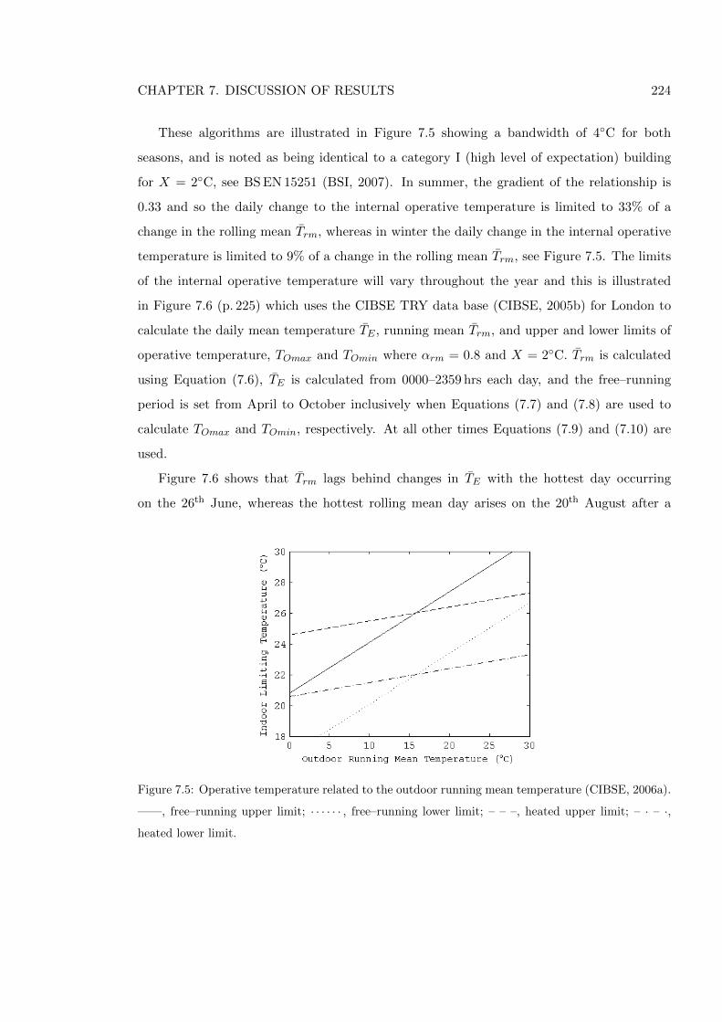
CHAPTER 7. DISCUSSION OF RESULTS 224
These algorithms are illustrated in Figure 7.5 showing a bandwidth of 4◦C for both
seasons, and is noted as being identical to a category I (high level of expectation) building
for X = 2◦C, see BS EN 15251 (BSI, 2007). In summer, the gradient of the relationship is
0.33 and so the daily change to the internal operative temperature is limited to 33% of a
change in the rolling mean Trm, whereas in winter the daily change in the internal operative
temperature is limited to 9% of a change in the rolling mean Trm, see Figure 7.5. The limits
of the internal operative temperature will vary throughout the year and this is illustrated
in Figure 7.6 (p. 225) which uses the CIBSE TRY data base (CIBSE, 2005b) for London to
calculate the daily mean temperature TE , running mean Trm, and upper and lower limits of
operative temperature, TOmax and TOmin where αrm = 0.8 and X = 2◦C. Trm is calculated
using Equation (7.6), TE is calculated from 0000–2359 hrs each day, and the free–running
period is set from April to October inclusively when Equations (7.7) and (7.8) are used to
calculate TOmax and TOmin, respectively. At all other times Equations (7.9) and (7.10) are
used.
Figure 7.6 shows that Trm lags behind changes in TE with the hottest day occurring
on the 26th June, whereas the hottest rolling mean day arises on the 20th August after a
Figure 7.5: Operative temperature related to the outdoor running mean temperature (CIBSE, 2006a).
——, free–running upper limit; · · · · · · , free–running lower limit; – – –, heated upper limit; – · – ·,
heated lower limit.
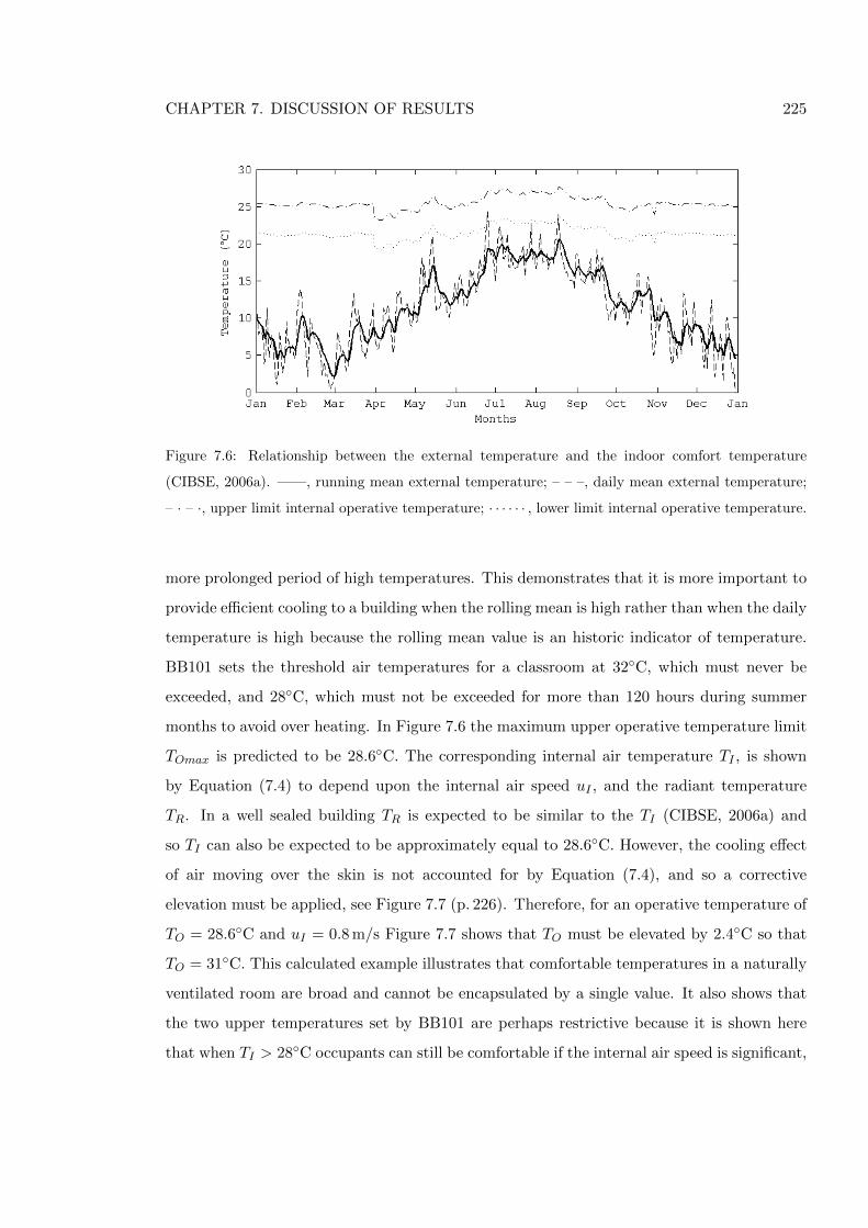
CHAPTER 7. DISCUSSION OF RESULTS 225
Figure 7.6: Relationship between the external temperature and the indoor comfort temperature
(CIBSE, 2006a). ——, running mean external temperature; – – –, daily mean external temperature;
– · – ·, upper limit internal operative temperature; · · · · · · , lower limit internal operative temperature.
more prolonged period of high temperatures. This demonstrates that it is more important to
provide efficient cooling to a building when the rolling mean is high rather than when the daily
temperature is high because the rolling mean value is an historic indicator of temperature.
BB101 sets the threshold air temperatures for a classroom at 32◦C, which must never be
exceeded, and 28◦C, which must not be exceeded for more than 120 hours during summer
months to avoid over heating. In Figure 7.6 the maximum upper operative temperature limit
TOmax is predicted to be 28.6◦C. The corresponding internal air temperature TI , is shown
by Equation (7.4) to depend upon the internal air speed uI , and the radiant temperature
TR. In a well sealed building TR is expected to be similar to the TI (CIBSE, 2006a) and
so TI can also be expected to be approximately equal to 28.6◦C. However, the cooling effect
of air moving over the skin is not accounted for by Equation (7.4), and so a corrective
elevation must be applied, see Figure 7.7 (p. 226). Therefore, for an operative temperature of
TO = 28.6◦C and uI = 0.8 m/s Figure 7.7 shows that TO must be elevated by 2.4◦C so that
TO = 31◦C. This calculated example illustrates that comfortable temperatures in a naturally
ventilated room are broad and cannot be encapsulated by a single value. It also shows that
the two upper temperatures set by BB101 are perhaps restrictive because it is shown here
that when TI > 28◦C occupants can still be comfortable if the internal air speed is significant,
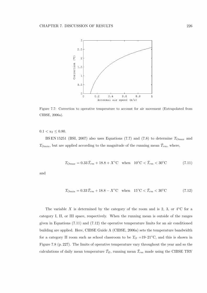
CHAPTER 7. DISCUSSION OF RESULTS 226
Figure 7.7: Correction to operative temperature to account for air movement (Extrapolated from
CIBSE, 2006a).
0.1 < uI ≤ 0.80.
BS EN 15251 (BSI, 2007) also uses Equations (7.7) and (7.8) to determine TOmax and
TOmin, but are applied according to the magnitude of the running mean Trm, where,
TOmax = 0.33 Trm + 18.8 +X◦C when 10◦C < Trm < 30◦C (7.11)
and
TOmin = 0.33 Trm + 18.8−X◦C when 15◦C < Trm < 30◦C (7.12)
The variable X is determined by the category of the room and is 2, 3, or 4◦C for a
category I, II, or III space, respectively. When the running mean is outside of the ranges
given in Equations (7.11) and (7.12) the operative temperature limits for an air conditioned
building are applied. Here, CIBSE Guide A (CIBSE, 2006a) sets the temperature bandwidth
for a category II room such as school classroom to be TO =19–21◦C, and this is shown in
Figure 7.8 (p. 227). The limits of operative temperature vary throughout the year and so the
calculations of daily mean temperature TE , running mean Trm made using the CIBSE TRY
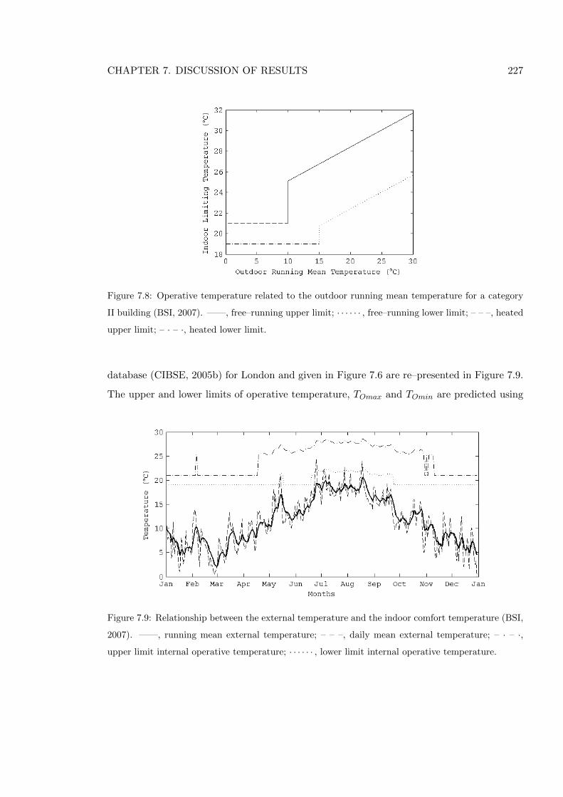
CHAPTER 7. DISCUSSION OF RESULTS 227
Figure 7.8: Operative temperature related to the outdoor running mean temperature for a category
II building (BSI, 2007). ——, free–running upper limit; · · · · · · , free–running lower limit; – – –, heated
upper limit; – · – ·, heated lower limit.
database (CIBSE, 2005b) for London and given in Figure 7.6 are re–presented in Figure 7.9.
The upper and lower limits of operative temperature, TOmax and TOmin are predicted using
Figure 7.9: Relationship between the external temperature and the indoor comfort temperature (BSI,
2007). ——, running mean external temperature; – – –, daily mean external temperature; – · – ·,
upper limit internal operative temperature; · · · · · · , lower limit internal operative temperature.
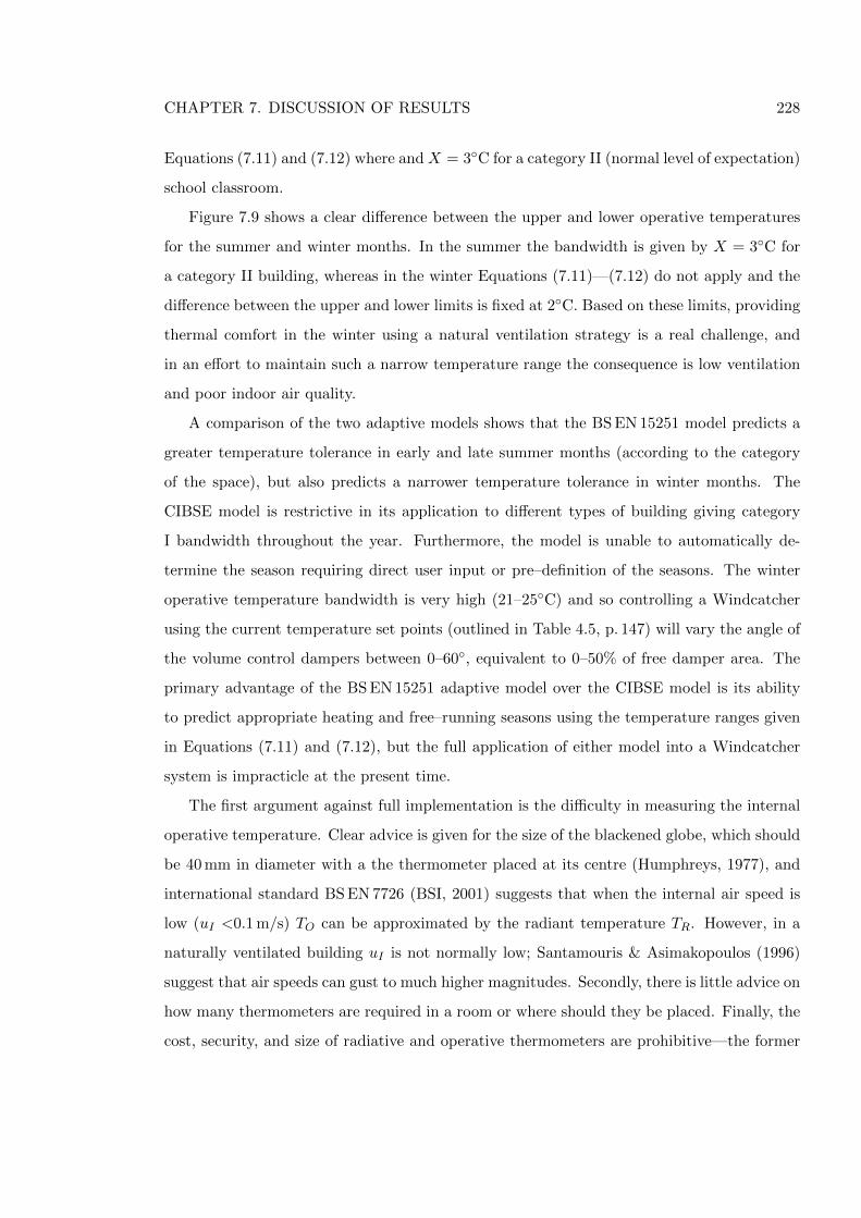
CHAPTER 7. DISCUSSION OF RESULTS 228
Equations (7.11) and (7.12) where and X = 3◦C for a category II (normal level of expectation)
school classroom.
Figure 7.9 shows a clear difference between the upper and lower operative temperatures
for the summer and winter months. In the summer the bandwidth is given by X = 3◦C for
a category II building, whereas in the winter Equations (7.11)—(7.12) do not apply and the
difference between the upper and lower limits is fixed at 2◦C. Based on these limits, providing
thermal comfort in the winter using a natural ventilation strategy is a real challenge, and
in an effort to maintain such a narrow temperature range the consequence is low ventilation
and poor indoor air quality.
A comparison of the two adaptive models shows that the BS EN 15251 model predicts a
greater temperature tolerance in early and late summer months (according to the category
of the space), but also predicts a narrower temperature tolerance in winter months. The
CIBSE model is restrictive in its application to different types of building giving category
I bandwidth throughout the year. Furthermore, the model is unable to automatically de-
termine the season requiring direct user input or pre–definition of the seasons. The winter
operative temperature bandwidth is very high (21–25◦C) and so controlling a Windcatcher
using the current temperature set points (outlined in Table 4.5, p. 147) will vary the angle of
the volume control dampers between 0–60◦, equivalent to 0–50% of free damper area. The
primary advantage of the BS EN 15251 adaptive model over the CIBSE model is its ability
to predict appropriate heating and free–running seasons using the temperature ranges given
in Equations (7.11) and (7.12), but the full application of either model into a Windcatcher
system is impracticle at the present time.
The first argument against full implementation is the difficulty in measuring the internal
operative temperature. Clear advice is given for the size of the blackened globe, which should
be 40 mm in diameter with a the thermometer placed at its centre (Humphreys, 1977), and
international standard BS EN 7726 (BSI, 2001) suggests that when the internal air speed is
low (uI <0.1 m/s) TO can be approximated by the radiant temperature TR. However, in a
naturally ventilated building uI is not normally low; Santamouris & Asimakopoulos (1996)
suggest that air speeds can gust to much higher magnitudes. Secondly, there is little advice on
how many thermometers are required in a room or where should they be placed. Finally, the
cost, security, and size of radiative and operative thermometers are prohibitive—the former
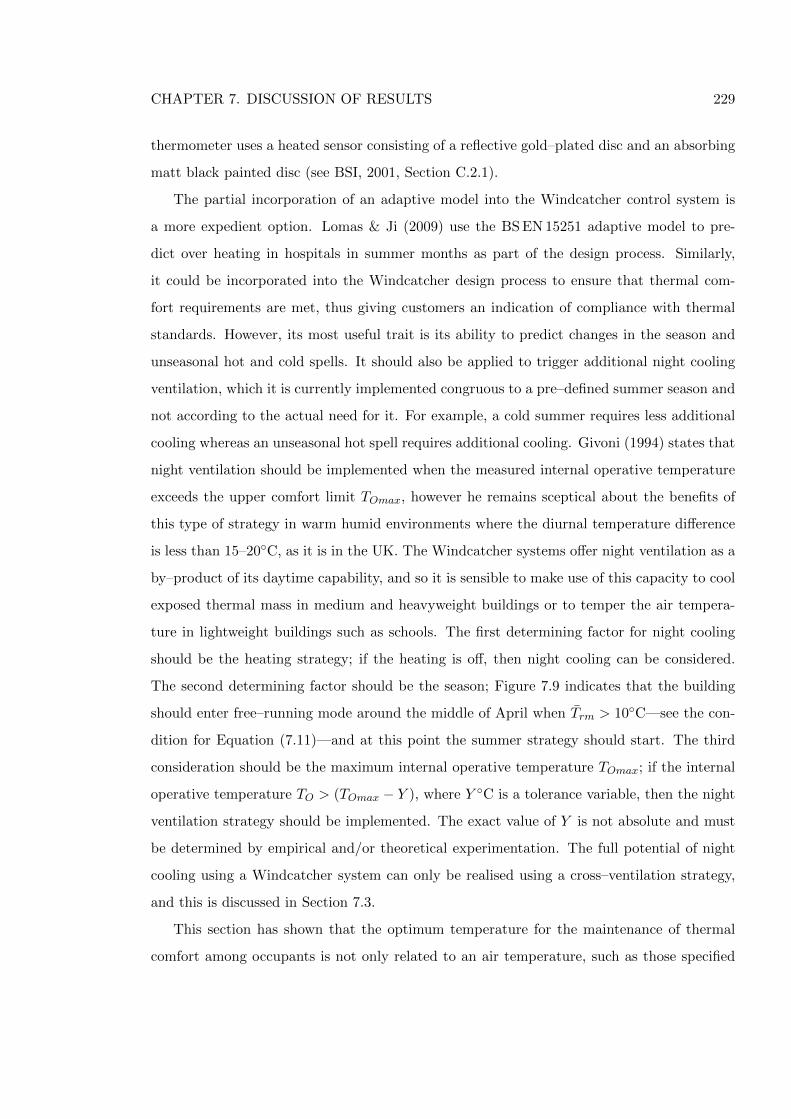
CHAPTER 7. DISCUSSION OF RESULTS 229
thermometer uses a heated sensor consisting of a reflective gold–plated disc and an absorbing
matt black painted disc (see BSI, 2001, Section C.2.1).
The partial incorporation of an adaptive model into the Windcatcher control system is
a more expedient option. Lomas & Ji (2009) use the BS EN 15251 adaptive model to pre-
dict over heating in hospitals in summer months as part of the design process. Similarly,
it could be incorporated into the Windcatcher design process to ensure that thermal com-
fort requirements are met, thus giving customers an indication of compliance with thermal
standards. However, its most useful trait is its ability to predict changes in the season and
unseasonal hot and cold spells. It should also be applied to trigger additional night cooling
ventilation, which it is currently implemented congruous to a pre–defined summer season and
not according to the actual need for it. For example, a cold summer requires less additional
cooling whereas an unseasonal hot spell requires additional cooling. Givoni (1994) states that
night ventilation should be implemented when the measured internal operative temperature
exceeds the upper comfort limit TOmax, however he remains sceptical about the benefits of
this type of strategy in warm humid environments where the diurnal temperature difference
is less than 15–20◦C, as it is in the UK. The Windcatcher systems offer night ventilation as a
by–product of its daytime capability, and so it is sensible to make use of this capacity to cool
exposed thermal mass in medium and heavyweight buildings or to temper the air tempera-
ture in lightweight buildings such as schools. The first determining factor for night cooling
should be the heating strategy; if the heating is off, then night cooling can be considered.
The second determining factor should be the season; Figure 7.9 indicates that the building
should enter free–running mode around the middle of April when Trm > 10◦C—see the con-
dition for Equation (7.11)—and at this point the summer strategy should start. The third
consideration should be the maximum internal operative temperature TOmax; if the internal
operative temperature TO > (TOmax − Y ), where Y ◦C is a tolerance variable, then the night
ventilation strategy should be implemented. The exact value of Y is not absolute and must
be determined by empirical and/or theoretical experimentation. The full potential of night
cooling using a Windcatcher system can only be realised using a cross–ventilation strategy,
and this is discussed in Section 7.3.
This section has shown that the optimum temperature for the maintenance of thermal
comfort among occupants is not only related to an air temperature, such as those specified
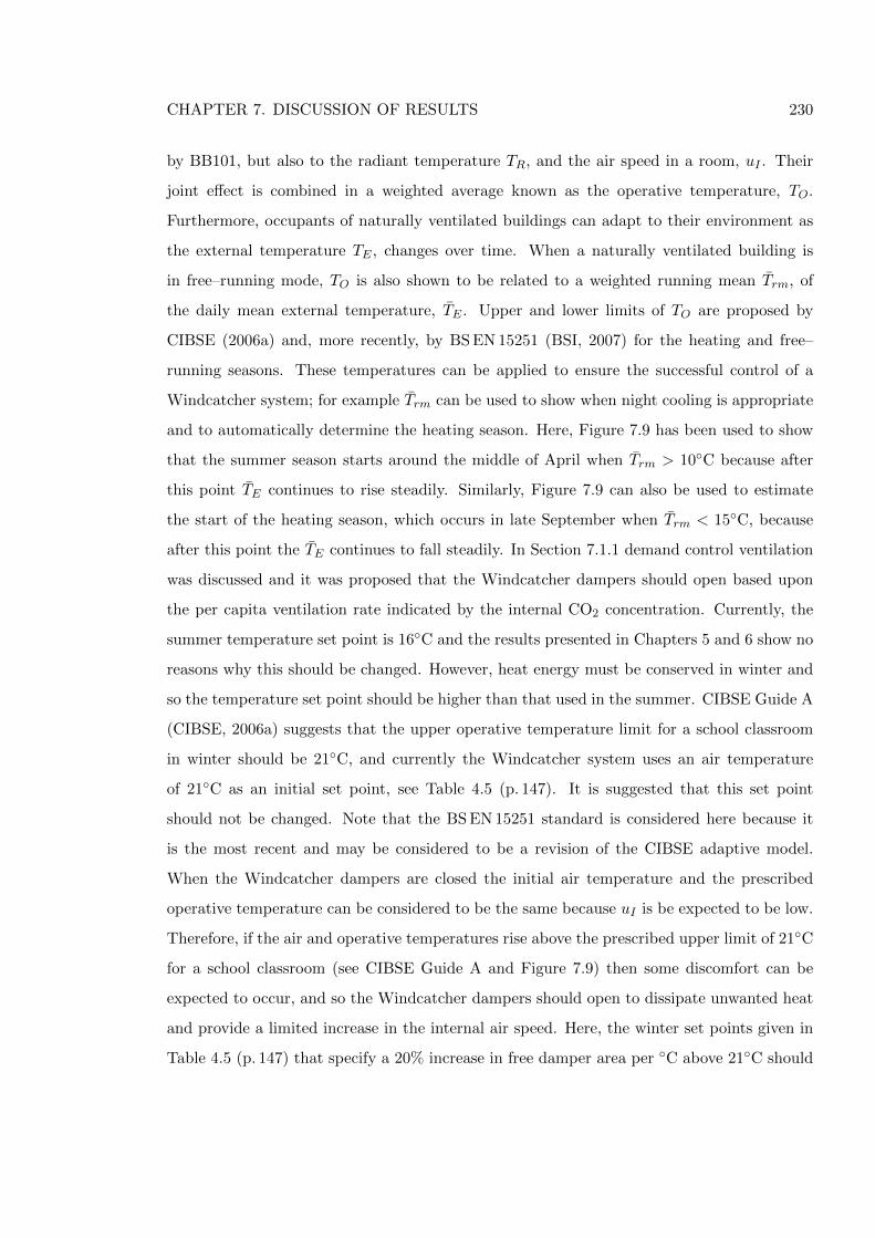
CHAPTER 7. DISCUSSION OF RESULTS 230
by BB101, but also to the radiant temperature TR, and the air speed in a room, uI . Their
joint effect is combined in a weighted average known as the operative temperature, TO.
Furthermore, occupants of naturally ventilated buildings can adapt to their environment as
the external temperature TE , changes over time. When a naturally ventilated building is
in free–running mode, TO is also shown to be related to a weighted running mean Trm, of
the daily mean external temperature, TE . Upper and lower limits of TO are proposed by
CIBSE (2006a) and, more recently, by BS EN 15251 (BSI, 2007) for the heating and free–
running seasons. These temperatures can be applied to ensure the successful control of a
Windcatcher system; for example Trm can be used to show when night cooling is appropriate
and to automatically determine the heating season. Here, Figure 7.9 has been used to show
that the summer season starts around the middle of April when Trm > 10◦C because after
this point TE continues to rise steadily. Similarly, Figure 7.9 can also be used to estimate
the start of the heating season, which occurs in late September when Trm < 15◦C, because
after this point the TE continues to fall steadily. In Section 7.1.1 demand control ventilation
was discussed and it was proposed that the Windcatcher dampers should open based upon
the per capita ventilation rate indicated by the internal CO2 concentration. Currently, the
summer temperature set point is 16◦C and the results presented in Chapters 5 and 6 show no
reasons why this should be changed. However, heat energy must be conserved in winter and
so the temperature set point should be higher than that used in the summer. CIBSE Guide A
(CIBSE, 2006a) suggests that the upper operative temperature limit for a school classroom
in winter should be 21◦C, and currently the Windcatcher system uses an air temperature
of 21◦C as an initial set point, see Table 4.5 (p. 147). It is suggested that this set point
should not be changed. Note that the BS EN 15251 standard is considered here because it
is the most recent and may be considered to be a revision of the CIBSE adaptive model.
When the Windcatcher dampers are closed the initial air temperature and the prescribed
operative temperature can be considered to be the same because uI is be expected to be low.
Therefore, if the air and operative temperatures rise above the prescribed upper limit of 21◦C
for a school classroom (see CIBSE Guide A and Figure 7.9) then some discomfort can be
expected to occur, and so the Windcatcher dampers should open to dissipate unwanted heat
and provide a limited increase in the internal air speed. Here, the winter set points given in
Table 4.5 (p. 147) that specify a 20% increase in free damper area per ◦C above 21◦C should
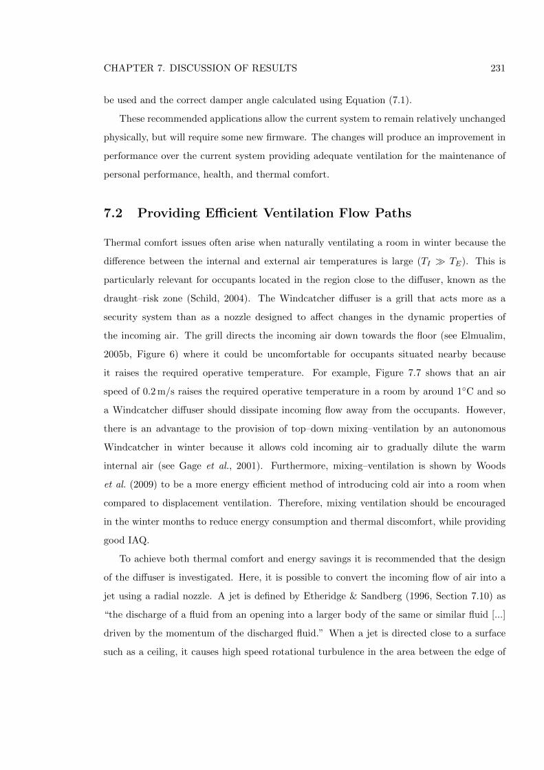
CHAPTER 7. DISCUSSION OF RESULTS 231
be used and the correct damper angle calculated using Equation (7.1).
These recommended applications allow the current system to remain relatively unchanged
physically, but will require some new firmware. The changes will produce an improvement in
performance over the current system providing adequate ventilation for the maintenance of
personal performance, health, and thermal comfort.
7.2 Providing Efficient Ventilation Flow Paths
Thermal comfort issues often arise when naturally ventilating a room in winter because the
difference between the internal and external air temperatures is large (TI � TE). This is
particularly relevant for occupants located in the region close to the diffuser, known as the
draught–risk zone (Schild, 2004). The Windcatcher diffuser is a grill that acts more as a
security system than as a nozzle designed to affect changes in the dynamic properties of
the incoming air. The grill directs the incoming air down towards the floor (see Elmualim,
2005b, Figure 6) where it could be uncomfortable for occupants situated nearby because
it raises the required operative temperature. For example, Figure 7.7 shows that an air
speed of 0.2 m/s raises the required operative temperature in a room by around 1◦C and so
a Windcatcher diffuser should dissipate incoming flow away from the occupants. However,
there is an advantage to the provision of top–down mixing–ventilation by an autonomous
Windcatcher in winter because it allows cold incoming air to gradually dilute the warm
internal air (see Gage et al., 2001). Furthermore, mixing–ventilation is shown by Woods
et al. (2009) to be a more energy efficient method of introducing cold air into a room when
compared to displacement ventilation. Therefore, mixing ventilation should be encouraged
in the winter months to reduce energy consumption and thermal discomfort, while providing
good IAQ.
To achieve both thermal comfort and energy savings it is recommended that the design
of the diffuser is investigated. Here, it is possible to convert the incoming flow of air into a
jet using a radial nozzle. A jet is defined by Etheridge & Sandberg (1996, Section 7.10) as
“the discharge of a fluid from an opening into a larger body of the same or similar fluid [...]
driven by the momentum of the discharged fluid.” When a jet is directed close to a surface
such as a ceiling, it causes high speed rotational turbulence in the area between the edge of
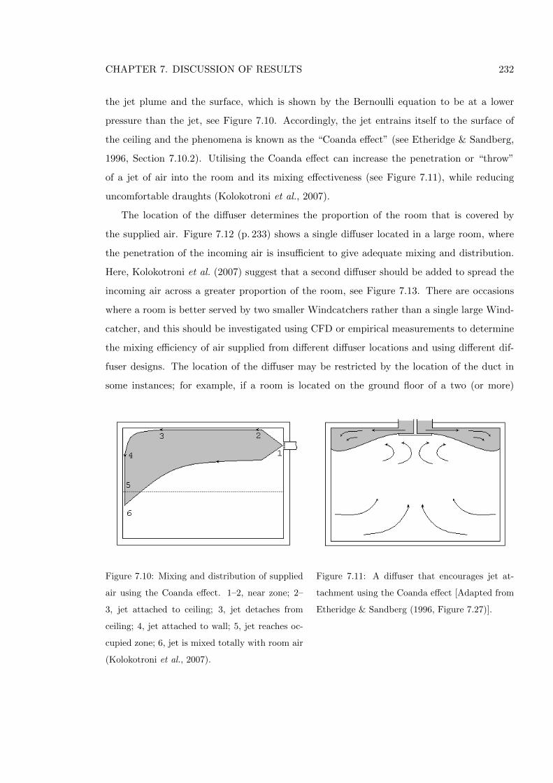
CHAPTER 7. DISCUSSION OF RESULTS 232
the jet plume and the surface, which is shown by the Bernoulli equation to be at a lower
pressure than the jet, see Figure 7.10. Accordingly, the jet entrains itself to the surface of
the ceiling and the phenomena is known as the “Coanda effect” (see Etheridge & Sandberg,
1996, Section 7.10.2). Utilising the Coanda effect can increase the penetration or “throw”
of a jet of air into the room and its mixing effectiveness (see Figure 7.11), while reducing
uncomfortable draughts (Kolokotroni et al., 2007).
The location of the diffuser determines the proportion of the room that is covered by
the supplied air. Figure 7.12 (p. 233) shows a single diffuser located in a large room, where
the penetration of the incoming air is insufficient to give adequate mixing and distribution.
Here, Kolokotroni et al. (2007) suggest that a second diffuser should be added to spread the
incoming air across a greater proportion of the room, see Figure 7.13. There are occasions
where a room is better served by two smaller Windcatchers rather than a single large Wind-
catcher, and this should be investigated using CFD or empirical measurements to determine
the mixing efficiency of air supplied from different diffuser locations and using different dif-
fuser designs. The location of the diffuser may be restricted by the location of the duct in
some instances; for example, if a room is located on the ground floor of a two (or more)
Figure 7.10: Mixing and distribution of supplied
air using the Coanda effect. 1–2, near zone; 2–
3, jet attached to ceiling; 3, jet detaches from
ceiling; 4, jet attached to wall; 5, jet reaches oc-
cupied zone; 6, jet is mixed totally with room air
(Kolokotroni et al., 2007).
Figure 7.11: A diffuser that encourages jet at-
tachment using the Coanda effect [Adapted from
Etheridge & Sandberg (1996, Figure 7.27)].
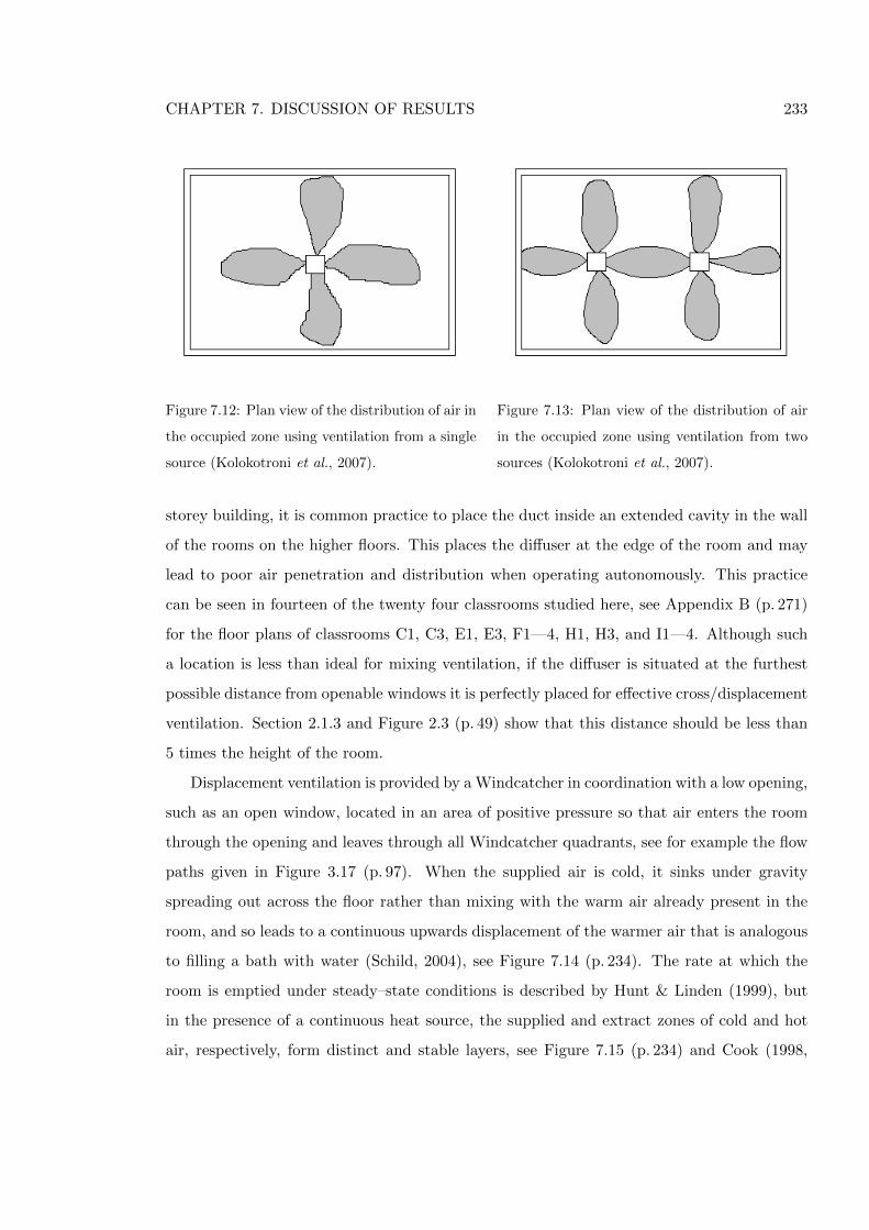
CHAPTER 7. DISCUSSION OF RESULTS 233
Figure 7.12: Plan view of the distribution of air in
the occupied zone using ventilation from a single
source (Kolokotroni et al., 2007).
Figure 7.13: Plan view of the distribution of air
in the occupied zone using ventilation from two
sources (Kolokotroni et al., 2007).
storey building, it is common practice to place the duct inside an extended cavity in the wall
of the rooms on the higher floors. This places the diffuser at the edge of the room and may
lead to poor air penetration and distribution when operating autonomously. This practice
can be seen in fourteen of the twenty four classrooms studied here, see Appendix B (p. 271)
for the floor plans of classrooms C1, C3, E1, E3, F1—4, H1, H3, and I1—4. Although such
a location is less than ideal for mixing ventilation, if the diffuser is situated at the furthest
possible distance from openable windows it is perfectly placed for effective cross/displacement
ventilation. Section 2.1.3 and Figure 2.3 (p. 49) show that this distance should be less than
5 times the height of the room.
Displacement ventilation is provided by a Windcatcher in coordination with a low opening,
such as an open window, located in an area of positive pressure so that air enters the room
through the opening and leaves through all Windcatcher quadrants, see for example the flow
paths given in Figure 3.17 (p. 97). When the supplied air is cold, it sinks under gravity
spreading out across the floor rather than mixing with the warm air already present in the
room, and so leads to a continuous upwards displacement of the warmer air that is analogous
to filling a bath with water (Schild, 2004), see Figure 7.14 (p. 234). The rate at which the
room is emptied under steady–state conditions is described by Hunt & Linden (1999), but
in the presence of a continuous heat source, the supplied and extract zones of cold and hot
air, respectively, form distinct and stable layers, see Figure 7.15 (p. 234) and Cook (1998,
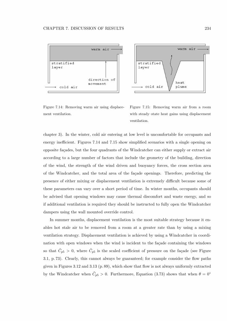
CHAPTER 7. DISCUSSION OF RESULTS 234
Figure 7.14: Removing warm air using displace-
ment ventilation.
Figure 7.15: Removing warm air from a room
with steady–state heat gains using displacement
ventilation.
chapter 3). In the winter, cold air entering at low level is uncomfortable for occupants and
energy inefficient. Figures 7.14 and 7.15 show simplified scenarios with a single opening on
opposite facades, but the four quadrants of the Windcatcher can either supply or extract air
according to a large number of factors that include the geometry of the building, direction
of the wind, the strength of the wind driven and buoyancy forces, the cross section area
of the Windcatcher, and the total area of the facade openings. Therefore, predicting the
presence of either mixing or displacement ventilation is extremely difficult because some of
these parameters can vary over a short period of time. In winter months, occupants should
be advised that opening windows may cause thermal discomfort and waste energy, and so
if additional ventilation is required they should be instructed to fully open the Windcatcher
dampers using the wall mounted override control.
In summer months, displacement ventilation is the most suitable strategy because it en-
ables hot stale air to be removed from a room at a greater rate than by using a mixing
ventilation strategy. Displacement ventilation is achieved by using a Windcatcher in coordi-
nation with open windows when the wind is incident to the facade containing the windows
so that Cp5 > 0, where Cp5 is the scaled coefficient of pressure on the facade (see Figure
3.1, p. 73). Clearly, this cannot always be guaranteed; for example consider the flow paths
given in Figures 3.12 and 3.13 (p. 89), which show that flow is not always uniformly extracted
by the Windcatcher when Cp5 > 0. Furthermore, Equation (3.73) shows that when θ = 0◦
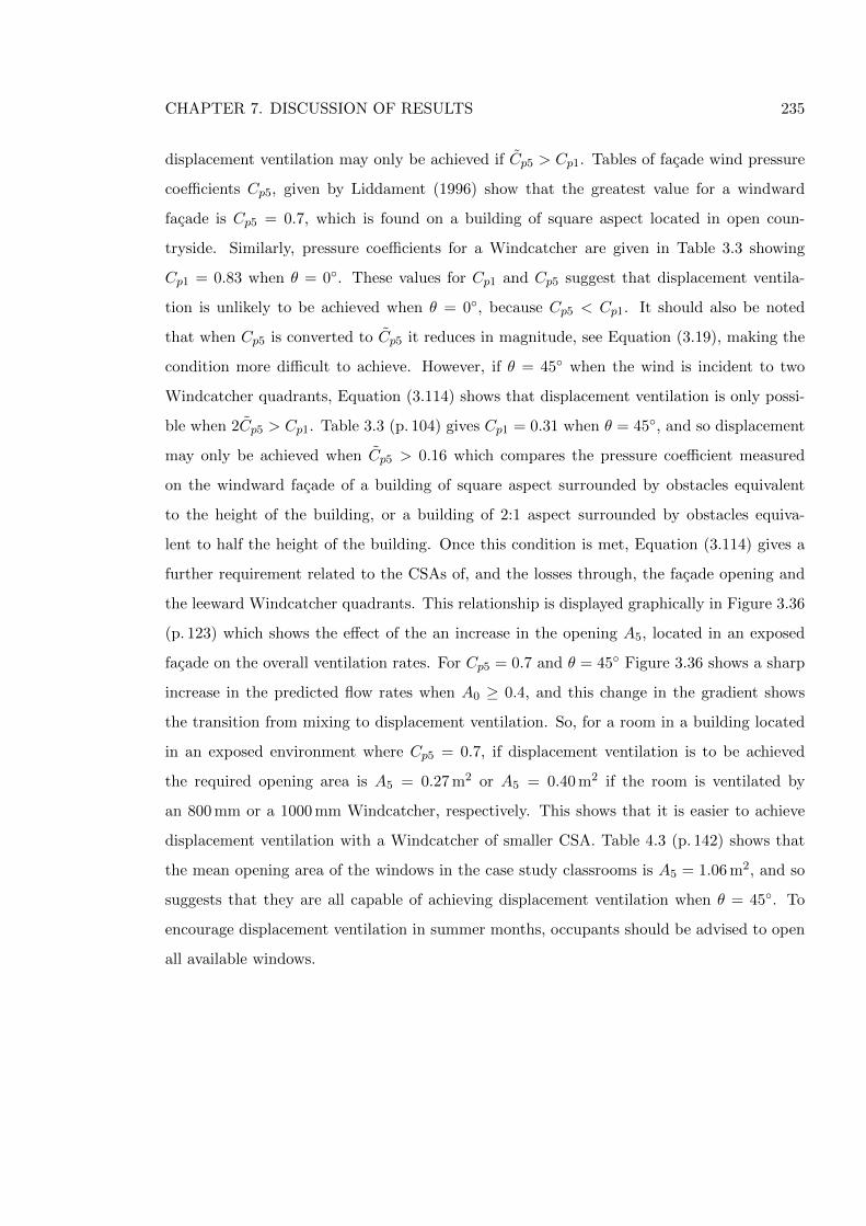
CHAPTER 7. DISCUSSION OF RESULTS 235
displacement ventilation may only be achieved if Cp5 > Cp1. Tables of facade wind pressure
coefficients Cp5, given by Liddament (1996) show that the greatest value for a windward
facade is Cp5 = 0.7, which is found on a building of square aspect located in open coun-
tryside. Similarly, pressure coefficients for a Windcatcher are given in Table 3.3 showing
Cp1 = 0.83 when θ = 0◦. These values for Cp1 and Cp5 suggest that displacement ventila-
tion is unlikely to be achieved when θ = 0◦, because Cp5 < Cp1. It should also be noted
that when Cp5 is converted to Cp5 it reduces in magnitude, see Equation (3.19), making the
condition more difficult to achieve. However, if θ = 45◦ when the wind is incident to two
Windcatcher quadrants, Equation (3.114) shows that displacement ventilation is only possi-
ble when 2Cp5 > Cp1. Table 3.3 (p. 104) gives Cp1 = 0.31 when θ = 45◦, and so displacement
may only be achieved when Cp5 > 0.16 which compares the pressure coefficient measured
on the windward facade of a building of square aspect surrounded by obstacles equivalent
to the height of the building, or a building of 2:1 aspect surrounded by obstacles equiva-
lent to half the height of the building. Once this condition is met, Equation (3.114) gives a
further requirement related to the CSAs of, and the losses through, the facade opening and
the leeward Windcatcher quadrants. This relationship is displayed graphically in Figure 3.36
(p. 123) which shows the effect of the an increase in the opening A5, located in an exposed
facade on the overall ventilation rates. For Cp5 = 0.7 and θ = 45◦ Figure 3.36 shows a sharp
increase in the predicted flow rates when A0 ≥ 0.4, and this change in the gradient shows
the transition from mixing to displacement ventilation. So, for a room in a building located
in an exposed environment where Cp5 = 0.7, if displacement ventilation is to be achieved
the required opening area is A5 = 0.27 m2 or A5 = 0.40 m2 if the room is ventilated by
an 800 mm or a 1000 mm Windcatcher, respectively. This shows that it is easier to achieve
displacement ventilation with a Windcatcher of smaller CSA. Table 4.3 (p. 142) shows that
the mean opening area of the windows in the case study classrooms is A5 = 1.06 m2, and so
suggests that they are all capable of achieving displacement ventilation when θ = 45◦. To
encourage displacement ventilation in summer months, occupants should be advised to open
all available windows.
CHAPTER 7. DISCUSSION OF RESULTS 236
7.3 Improving the Windcatcher System
Table 3.5 on (p. 111) shows the predicted loss coefficients for a Windcatcher. The component
that is estimated to cause the greatest losses in the Windcatcher system is the top (louvred)
section, which converges, turns, and then diverges the flow of air as it enters the Windcatcher
element. Losses in this section have to be balanced against the ingress of rain and debris, and
their design has evolved over time to avoid this. Therefore, any changes aimed at lowering the
head loss through this section are likely to increase the amount of rain and debris that enters
through the louvres, which would be commercially unsatisfactory. Moreover, the addition
of fittings designed to reduce head loss are unlikely to be of benefit. For example, turning
vanes (see CIBSE, 2001) are designed to avoid the formation of eddies in an elbow, but would
require modification to fit into the Windcatcher’s triangular ducts. Their efficiency increases
with higher flow rates, but because the Windcatcher is subject to gusts of wind and the air
speed is relatively low in the ducts (see Figure 3.21, p. 105), the addition of turning vanes
is very likely to be unsuccessful in consistently lowering the head loss. Consideration should
also be given to the cost of installing precision fittings such as vanes because the Windcatcher
is designed to be a relatively low cost–natural ventilation system, and so capital spent to gain
relatively small reductions in head loss will compromise this business model.
One of the major issues highlighted in Chapter 6 is the reduced performance of au-
tonomous Windcatchers with duct lengths greater than 1 m. It has been suggested in Section
6.1 (p. 186) that this is due to the short length of the partition, which does not extend for
the full length of the duct. Consequently, the supplied air is simply taking the path of least
resistance and is extracted by the Windcatcher through the leeward quadrants long before
it reaches the room. Evidence for this is provided by the CFD analysis of Hughes & Ghani
(2008, Figures 10 and 13) who show that short circuiting occurs between the area between
the bottom of the partition and the top of the open dampers. To increase bi–directional flow
through a Windcatcher and, therefore, to increase total ventilation rates through a room, the
solution is to partition the ducts along their whole length. However, Hughes & Ghani (2008)
show that short circuiting occurs even when the duct length is apparently short; the duct
length is not given but diagrams intimate that they tested a duct with a length that was
approximately 33% of the total element height. This suggests that if the partition is extended
CHAPTER 7. DISCUSSION OF RESULTS 237
to cover the whole length of a duct, then short circuiting will occur no matter how long the
duct is. The source of this problem is the gap between the partition and the dampers. A
solution is to remove this gap by connecting the partition directly to the diffuser. Clearly,
this requires the removal of the dampers and eliminates the ability to control the volume
of air entering a room, which is unsatisfactory. Another solution is a reduction in the gap
loacted between the dampers and the diffuser so that when the dampers are fully open they
are flush to both components.
Yet another possibility is to control the flow of air elsewhere, and here the Windcatcher
element louvres could be used. A system of movable louvres would control air into the element
in the same way that venetian blinds vary the amount of light entering a room through a
window. When used with a rain sensor, the louvres would close in bad weather sealing
the Windcatcher protecting the supplied room from rain, hail, sleet, or snow. Moreover,
this would allow the louvres to be completely redesigned so that they are aerodynamically
more efficient. A notable drawback in winter months is heat loss, and although this is to
be expected when the Windcatcher is actively ventilating, unnecessary heat loss will occur
through the duct to the loft cavity and the Windcatcher element when the Windcatcher is
intentionally inactive and the the louvres are closed. Here, the duct can be lagged, but an
efficient seal at ceiling level using dampers may still be required to avoid heat loss through
the Windcatcher element.
The Windcatcher system is marketed and sold as a top–down ventilation system but the
in–situ measurements and the semi–empirical predictions show that a Windcatcher used in
coordination with facade openings can double the ventilation rate, see Section 6.2 (p. 191).
In Section 7.1.1 the use of automatically opening windows was proposed to provide purge
ventilation at break times or at night. Adding facade openings to the existing flow paths
would accord greater control of the system and allow it to cope with deviations from the
design criteria. There are security issues when opening windows at night and so an alternative
is to use a duct through the facade wall protected by a security grill, see Cook & Short (2005).
The volume of air though the opening is then controlled using a damper arrangement similar
to that used by the Windcatcher, but with significantly improved insulating properties so that
they conform to thermal and pressure test standards. The Queens Building at De Montfort
University uses a retro–fitted radiator array in front of the opening to temper incoming air
CHAPTER 7. DISCUSSION OF RESULTS 238
in winter months, however Section 7.2 shows that it is not simple to predict the direction of
the flow through the opening and so it is highly likely that this solution is inefficient for a
Windcatcher system and should only be used in summer months. Then, it would significantly
improve the ability of the Windcatcher system to perform night cooling, particularly when
wind speeds are low.
7.4 Application of the Windcatcher to Other Non–Domestic
Building Types
This thesis has explored the use of Windcatchers in schools, and specifically in school class-
rooms. The characteristics of a school classroom are reported in Chapter 4 and show that
occupancy densities are very high when compared to other non–domestic building types such
as offices (Clements-Croome et al., 2008), and so a Windcatcher ventilation system must
deliver a greater net ventilation rate to a classroom than is required by another type of room,
such as an office. Accordingly, it can be reasoned that because a carefully designed Wind-
catcher system has been shown to provide sufficient ventilation to a classroom under specific
conditions (see Chapters 5 and 6), it can also ventilate other non–domestic building types
where the required net ventilation is lower; for example, offices, factories, and retail outlet all
require 10 l/s – person (see CIBSE, 2006a) but have lower occupancy densities. However, the
biggest opportunity for future applications of Windcatcher systems is likely to remain within
the public sector because the British Government is committed to take action against climate
change which includes a major reduction in energy consumption, see the NHS Carbon Reduc-
tion Strategy for England for example (NHS, 2009). It is highly likely that Windcatchers will
continue to be installed in schools because the school construction programme will continue
until 2020 (Mumovic et al., 2009), see Section 2.1.2 (p. 34).
A further opportunity lies in healthcare buildings; the National Health Service (NHS) is
the largest employer in Europe employing 1.3 million people and 5% of the UK work force. It
currently occupies and manages 14,040 sites and is responsible for 3% of all UK CO2 emissions
and 30% of all public sector emissions. Approximately 44% of energy consumed in a typical
NHS hospital is used for air and space heating and so one may expect climatic warming to
lead to reduced consumption in winter months. However, an assessment of energy consumed
CHAPTER 7. DISCUSSION OF RESULTS 239
between 1999 and 2005 shows that overall consumption increased by 7% per annum; see
Lomas & Ji (2009) for references of all figures. At this rate of growth, and at fixed prices,
its energy costs are likely to double every 10 years. Accordingly, the Department of Health
(DoH) has set stringent energy targets for all new and refurbished buildings and an energy
reduction target of 15% from 2000 to 2010; a target which the NHS trusts are struggling
to meet (NHS, 2009). Most NHS trust buildings are not air conditioned, which helps to
reduce their energy demand, but renders their buildings potentially susceptible to climate
change. Whereas healthy occupants can adapt to higher than normal temperatures and to
heat waves, this is not necessarily so for the the occupants of a hospital who are sick, confined
to bed, or have suppressed thermoregulatory systems. Furthermore, hospitals must provide
a comfortable working environment for staff who may be involved in life threatening work.
The challenge of reconciling the competing demands of curbing energy use and improving
resilience to climate change is one that must be met by modern hospitals and the building
services products that they employ.
A recent health technical memorandum (DoH, 2007) states that “natural ventilation is
always the preferred solution for a space, provided that the quantity and quality of air re-
quired, and the consistency of control to suit the requirements of the space, are achievable.”
Some concern over airborne disease and cross infection in naturally ventilated buildings has,
in the past, been a driver for the installation of mechanical ventilation systems in healthcare
premises (NHS, 2009). However, current academic research suggests that there are a number
of coexisting factors that can contribute to infection transmission and so it is difficult to com-
pletely rule out the possibility of transmission by routes unrelated to the type of ventilation,
or to quantify the impact of ventilation on infection transmission rates (Li et al., 2007). It
is also suggested by the Patient Safety Agency that “true airborne infection is rare, what is
fairly common is the direct route of infection” (Short & Al-Maiyah, 2009). In fact, there is
growing concern about the healthiness of many mechanical ventilation systems because poor
indoor air quality and unhygienic air supply conditions have been directly associated with
poor maintenance (Roaf, 2007). In addition, pressurised mechanical ventilation systems have
been linked in scientifically robust studies to the spread of a range of infectious diseases (Ku-
mari et al., 1998; Cotterill et al., 1996). Clearly, there is scope to employ natural ventilation
intelligently and a study by Short & Al-Maiyah (2009) suggests that up to 70% of net floor
CHAPTER 7. DISCUSSION OF RESULTS 240
area could be wholly or partly naturally ventilated.
Following the formation of the NHS Sustainable Development Unit (NHSSDU) and re-
cent consultation with NHS stakeholders, it is recommended by Short & Al-Maiyah (2009)
that displacement ventilation is used for clinical areas and mixing ventilation is reserved
for non–clinical areas. Accordingly, a Windcatcher system should only be installed in non–
clinical areas because it provides mixing ventilation when operating autonomously and pure
displacement ventilation cannot be guaranteed when it is used in coordination with facade
openings.
7.5 Immediate Application of this Work
Monodraught Ltd. are currently the market leader in the design and manufacture of ad-
vanced (top–down) natural ventilation systems for non–domestic buildings. It has sought to
stay ahead of the competition by commissioning small pieces of academic work from Brunel
(Kirk & Kolokotroni, 2004b; Kirk, 2004a), Reading (Elmualim & Awbi, 2002a), and Not-
tingham (Su et al., 2008) Universities to investigate the performance of the Windcatcher
system. Moreover, the research given here is now part of a long term company strategy that
puts research at its core. Previously sales have driven the research, but now the opposite is
true. This includes the way that Windcatcher strategies are designed and tendered. With
increased market place competition and a desire by customers to be given more information,
this strategy makes complete sense. For example, the steady–state semi–empirical model de-
scribed in Chapter 3 and corroborated in Chapter 6 is now central to the Monodraught design
strategy. It was shown in Section 6.3 that by applying weather data suitable for analysing
the environmental performance of buildings, the semi–empirical model can be used to predict
ventilation rates over a period of time, thus becoming a quasi–dynamic model. This idea
is now being implemented further by applying the semi–empirical model to an independent
steady–state thermal model (not discussed here), which when used in conjunction with TRY
and DRY weather data (CIBSE, 2005b) will also make quasi–dynamic predictions.
It is predicted that this knowledge, which has been derived independently from Mon-
odraught, and with academic rigor, will have a positive impact by
• Giving context to Windcatcher systems and their performance (see Chapters 1 and 2);
CHAPTER 7. DISCUSSION OF RESULTS 241
• Quantifying the performance of a Windcatcher system in–situ (see Chapters 4, 5, and
7);
• Predicting the performance of a Windcatcher system and corroborating the predictions
using measurements made in–situ (see Chapters 3 and 6);
• Presenting a simple, straight forward design process (see Chapter 6);
• Showing how the Windcatcher system can be used effectively and efficiently according
to the season (see Chapter 7), which will lead to improved performance;
• Identifying future development work and research projects (see Chapters 7 and 9);
• Invoking confidence in stakeholders when specific claims about the Windcatcher system
are made;
• Producing marketing material;
• Contributing to increased sales.
When tendering Windcatcher strategies for UK buildings there is an increasing number
of requirements to be met, and this is particularly so for school buildings. The statutory
requirements have been discussed in Chapter 2 and the Windcatcher performance compared
against them throughout this document. However, school designs now have to be reviewed
by the Commission for Architecture and the Built Environment CABE (2009a,b,c) and must
achieve a very good rating when assessed against the Buildings Research Establishment En-
vironmental Assessment Method (BREEAM) criteria. BREEAM (BRE, 2008) is a measure
of sustainability made at the design stage and credit is earned by implementing natural
ventilation systems where possible. However, it remains only an aspiration because it does
not close the loop by testing the performance of the building, although the presence of the
measures that earned credits at the design stage are checked when the building is handed
over. There may be many buildings that have received a very good rating but there is no
indication that they achieve the awarded level of performance and sustainability in practice.
The post occupancy assessment of the Windcatcher technology given here shows that if it is
implemented using the methodology outlined in Section 6.3.1 then the building will conform
CHAPTER 7. DISCUSSION OF RESULTS 242
to the current standards. Furthermore, the expertise in measuring a Windcatcher system
in–situ, developed during this project, can be applied if the loop is ever closed and the post
occupancy assessment of a building and its systems becomes mandatory.
CHAPTER 8. CONCLUSIONS 243
Chapter 8
Conclusions
The research has made a number of significant advances in the understanding of the perfor-
mance of a natural ventilation Windcatcher. These conclusions are made in an order that
allow direct comparison, where applicable, against the objectives of this thesis (see Section
1.5).
An analysis of existing literature that investigates Windcatcher performance empirically
and theoretically is used to quantify and understand the performance of a Windcatcher. The
flow rates one may expect through a Windcatcher and the coefficient of pressure on each
Windcatcher face are identified and an assessment of the accuracy of this data is made.
A semi–empirical model is developed that combines a simple analytic model with ex-
perimental data reported in the literature. It is shown to perform well against a range of
experimental data and CFD predictions and can be used as a quick iterative design tool.
With this in mind, a simple expression for extract ventilation rates is proposed that neglects
buoyancy effects, and so provides fast estimates of Windcatcher performance requiring no
computational effort. The semi–empirical model predicts ventilation rates through a room
ventilated by a Windcatcher in coordination with open windows, and estimates that this
configuration is capable of significantly improving ventilation rates over and above those pro-
vided by an autonomous Windcatcher, and of delivering those rates typically required by
building regulations in the UK.
Measurements of IAQ, ventilation, and noise made in twenty four classrooms of seven
UK schools show that that a Windcatcher is generally capable of meeting the requirements
CHAPTER 8. CONCLUSIONS 244
of UK standards BB101 and BB93. In summer months all classrooms met the CO2 require-
ments indicating sufficient per capita ventilation. Measurements of the ventilation rate in
each classroom with a Windcatcher operating autonomously show that 40% of measured
classrooms meet the minimum 3 l/s – person requirement and 23% meet the 5 l/s – person
requirement. If the Windcatcher is used in coordination with open windows, then all class-
rooms meet the 3 l/s – person requirement, 94% meet 5 l/s – person, and 77% meet 8 l/s –
person under this arrangement. Furthermore, for the classrooms studied here, it is evident
that a Windcatcher can aid in the delivery of ventilation rates that meet the UK standards
during the summer time and this also extends to meeting European and US standards. How-
ever, the Windcatcher is rarely open during the winter months and although the maximum
CO2 limit of 5000 ppm is never reached, only 62% of classrooms meet the required mean
CO2 level of 1500 ppm. Measurements of ambient noise in twenty three classrooms with the
Windcatcher dampers open suggest that the classrooms generally conform to BB93, although
the sample size is relatively small and so there is probably insufficient data to conclude that
Windcatchers do not represent a problem when meeting noise targets in schools. Finally, a
Windcatcher is shown to offer the potential to significantly improve natural ventilation rates
in school classrooms and to help them comply with IAQ standards for UK schools.
The predictions of ventilation rate by the semi–empirical model generally agree with those
measured in–situ, but with three notable exceptions for a room ventilated by an autonomous
Windcatcher. Firstly, ventilation rates are sometimes over–predicted. Secondly, the measured
volume flow rates do not exceed 0.23 m3/s, and appear to plateau when uw ≥ 2 m/s. This is
not predicted by the model and its cause is unclear. Thirdly, Windcatchers with long duct
sections exhibit relatively poor performance and this was also not predicted by the model.
In addition, when the Windcatcher is used in coordination with open windows the semi–
empirical model tends to under–predict the ventilation rates. The experimental analysis of
the Windcatcher demonstrates that Windcatcher performance can be significantly improved
by the addition of open windows to a room, thus confirming the earlier theoretical prediction.
This aspect is likely to help rooms ventilated by a Windcatcher meet ventilation standards
for buildings, such as BB101 in the UK. In these circumstances the careful selection of Cp
for a building is important for the accuracy of the semi–empirical predictions.
Typical wind conditions given by the CIBSE TRY weather series are applied to the semi–
CHAPTER 8. CONCLUSIONS 245
empirical model to predict the ventilation performance of a room ventilated by a Windcatcher
over any period of time, and is shown to be a useful design tool. It also identifies situations
where the wind speed is negligible, and here the Windcatcher system must rely on buoyancy
forces to generate ventilation through a room. When the semi–empirical model is used to
investigate this situation, the unsealed model is found to be unsuitable for situations where
uw → 0 m/s and |∆T | > 0◦C. Instead, the sealed model may be used to estimate ventilation
rates under these circumstances and although the predictions seem plausible, they remain
uncorroborated by empirical measurement. Here, the predictions suggest that an autonomous
Windcatcher is capable of providing minimum ventilation rates specified by BB101 for a class
of 30 occupants, and a Windcatcher in coordination with open windows could provide the
required minimum, mean, and purge ventilation rates. The investigation of the capabilities
of the semi–empirical model has enabled the development of a series of steps that a designer
can use to correctly size a Windcatcher for a particular application.
CHAPTER 9. FURTHER WORK 246
Chapter 9
Further Work
This chapter proposes further work based upon the analysis of Windcatcher performance
presented in Chapters 2—7. Firstly, Section 2.3.2 highlights several key problems with the
existing empirical measurements of a Windcatcher made in a wind tunnel. Therefore, the
following research should be undertaken to:
• Re–evaluate the performance of a square Windcatcher ventilating a sealed room under
controlled conditions, such as those experienced in a wind tunnel. Here, the equipment
should be updated to use omni–directional velocity sensors, such as hot–wire anemome-
ters, and state of the art pressure sensors.
• Extend the empirical analysis to re–analyse the performance of a Windcatcher with
circular geometry, with and without fins.
Secondly, Chapters 6 and 7 shows gaps in the current knowledge of Windcatcher performance,
and so research should be undertaken in the following areas:
• Investigate the reduced performance of a Windcatcher with a long duct section to
determine the capability of a Windcatcher to provide bi–directional flow in these cir-
cumstances. Here, the partition should be extended for the full length of the duct and
the possibility of connecting the partition to the diffuser should be considered.
• Quantify the flow attenuation of the volume control dampers for different free areas
and angles.
CHAPTER 9. FURTHER WORK 247
• Investigate Windcatcher performance for buoyancy driven ventilation establishing flow
paths and flow rates for varying ∆T .
• Determine methods of quickly calculating the coefficient of pressure (Cp5) on the facade
of a building to help increase the accuracy of the predictions of the semi–empirical model
for a Windcatcher ventilating a room in coordination with facade openings.
Thirdly, Chapter 7 suggests improvements to the Windcatcher system and identifies gaps in
the current knowledge of Windcatcher performance. Therefore, further research should be
undertaken in the following areas:
• The design of a diffuser to provide the efficient mixing of incoming air should be inves-
tigated, and should utilising the Coanda effect.
• The current louvre profile of a square Windcatcher has evolved to reduce the intake
of water, debris, birds, and insects. The ability to seal the louvres in adverse weather
would allow the most aerodynamic louvre profile to be used and eliminate the ingress of
foreign bodies. Here, this research may utilise aerodynamic fins to increase the negative
pressure areas on side and leeward Windcatcher faces.
Fourthly, Chapter 5 suggests that there is “probably insufficient data to conclude that Wind-
catchers do not represent a problem when meeting noise targets in schools.” Accordingly, the
following research into the acoustic properties of a Windcatcher system is proposed:
• Further measurements of continuous sound pressure levels measured over 30 minutes,
in accordance with BB93, would help to provide a firm conclusions.
• This study concentrates on the comparison of noise transmission through a Windcatcher
with the volume control dampers open and closed. The noise transmitted by open win-
dows would provide a useful counterpoint to the data provided here by comparing the
noise transmitted through a Windcatcher system with conventional ventilation open-
ings.
• Further testing is required that includes a detailed acoustic analysis of the Windcatcher
in–situ using the frequency domain. This would help to determine the frequencies that
CHAPTER 9. FURTHER WORK 248
are most readily transmitted from the surroundings into a room by a Windcatcher
system. Furthermore, Section 2.1.4 shows that the polyurethane foam acoustic used to
line Windcatcher duct sections is designed to attenuate mid and high frequencies and
is expected to have mixed effects on low frequency traffic noise. This could also be
quantified by a frequency analysis.
Finally, Chapter 5 shows that the Windcatcher is closed for the majority of the time in
winter months. Consequently , Chapter 7 recommends the use of a demand control system
that opens the Windcatcher volume control dampers according to the number of occupants
present in a room, thus ensuring that per capita flow rates are provided. The following further
research is proposed:
• Develop a suitable demand control natural ventilation system and test its performance
by measurement and modeling. Here, an intervention testing methodology should be
used to compare the performance of (i) a system offering no ventilation (ii) a tempera-
ture controlled system (iii) a demand controlled CO2 based system. (iv) a demand and
thermally controlled CO2 and temperature based system. The performance in the sum-
mer and winter months should be verified and heat losses in winter shown by accurate
modeling of the measured conditions using thermal modeling and CFD software.
• Further investigation into the measurement of the external temperature and the cal-
culation of a rolling mean temperature is required. This would enable seasonal switch
points to be incorporated into the control algorithm giving flexibility; for example, the
Windcatcher would be able to adapt to an Indian summer, or provide night–cooling
only when it is required to do so.
• Chapter 6 shows that the the most efficient ventilation strategy is that provided by a
Windcatcher in coordination with facade openings such as windows. The addition of
automatically opening windows, controlled by the Windcatcher system, would provide
highly effective cross–ventilation for summer time heat dissipation and night cooling,
see Chapter 7.
REFERENCES 249
References
Ackermann, ME. 2002. Cool Comfort: America’s Romance with Air Conditioning. Washing-
ton and London: Smithsonian Institution Press.
Andersen, A, & Hopkins, C. 2005. Sound Measurements and Natural Ventilation in Schools.
International Journal of Ventilation, 4(1), 57–70.
ANSI. 2002. ANSI Acoustical Performance Criteria, Design Requirements, and Guidelines
for Schools (S12.60–2002). Tech. rept. American National Standards Institute.
Apte, MG, Fisk, WJ, & Daisey, JM. 2000. Associations Between Indoor CO2 Concentrations
and Sick Building Syndrome Symptoms in U.S. Office Buildings: An Analysis of the 1994–
1996 BASE Study Data. Indoor Air, 10(4), 246–257.
ASHRAE. 2007. ANSI/ASHRAE Standard 62.1: Ventilation for Acceptable Indoor Air Qual-
ity. Atlanta, USA: American Society of Heating, Refrigeration, and Air–Conditioning En-
gineers.
Auliciems, A. 2001. Towards a Psycho–Physiological Model of Thermal Perception. Interna-
tional Journal Biometeorology, 25(2), 109–122.
Awbi, HB, & Elmualim, AA. 2002. Full Scale Model Windcatcher Performance Evaluation
Using a Wind Tunnel. In: World Renewable Energy Conference VII.
Aynsley, R. 2008. Quantifying the Cooling Sensation of Air Movement. International Journal
of Ventilation, 7(1), 67–76.
Bahadori, Mehdi N. 1994. Viability of wind towers in achieving summer comfort in the hot
arid regions of the middle east. Renewable Energy, 5(5-8), 879–892.
REFERENCES 250
Bailey, C. 2009. Learning from passive action. CIBSE Journal, 1(6), 28–31.
Bako-Biro, Z. 2004. Human Perception, SBS Symptoms and Performance of Office Work
During Exposure to Air Polluted by Building Materials and Personal Computers. Ph.D.
thesis, Technical University of Denmark.
Bako-Biro, Z, Wargocki, P, Weschler, CJ, & Fanger, PO. 2004. Effects of Pollution from
Personal Computers on Perceived Air Quality, SBS Symptoms and Productivity in Offices.
Indoor Air, 14(3), 178–187.
Bako-Biro, Z, Kochhar, N, Clements-Croome, DJ, Awbi, HB, & Williams, M. 2008. Ventila-
tion Rates in Schools and Pupil’s Performance Using Computerised Assessment Tests. In:
Indoor Air 2008.
Bartlett, KH, Martinez, M, & Bert, J. 2004. Modeling of Occupant–Generated CO2 Dynamics
in Naturally Ventilated Classrooms. Journal Of Occupational and Environmental Hygeine,
1(3), 139–148.
Beisteiner, A, & Coley, DA. 2002. Carbon Dioxide Levels and Summertime Ventilation Rates
in UK Schools. International Journal of Ventilation, 1(3), 181–187.
Boyer, H, Lauret, AP, Adelard, L, & Mara, TA. 1999. Building Ventilation: A Pressure
Airflow Model Computer Generation and Elements of Validation. Energy and Buildings,
29(3), 283–292.
Brager, GS, & De Dear, RJ. 1998. Thermal Adaptation in the Built Environment: A Liter-
ature Review. Energy and Buildings, 27(1), 83–96.
Brager, GS Schiller, & De Dear, RJ. 2000. A Standard for Natural Ventilation. ASHRAE
Journal, 42(10), 21–28.
BRE. 2005 (24th March 2005). Test Report: Laboratory Sound Insulation of Monodraught
G.R.P. Square Windcatcher System. Private Report 222354. Buildings Research Estab-
lishment.
BRE. 2008. BRE Environmental and Sustainability. Tech. rept. BRE.
REFERENCES 251
BSI. 1991. BS 5925. Code of Practice for Ventilation Principles and Designing for Natural
Ventilation. Tech. rept. BSI.
BSI. 2001. BS EN 7726. Ergonomics of the thermal environment. Instruments for measuring
physical quantities. Tech. rept. BSI.
BSI. 2004. BS EN 13779. Ventilation for Non–Residential Buildings — Performance Require-
ments for Ventilation and Room–Conditioning Systems. Tech. rept. BSI.
BSI. 2007. BS EN 15251. Indoor Environment Input Parameters for Design and Assessment
of Energy Performance of Buidlings Addressing Indoor Air Quality, Thermal Environment,
Lighting and Acoustics. Tech. rept. BSI.
CABE. 2009a. Effective School Design — Effective Graphic Approaches. Tech. rept. Com-
mission for Architecture and the Built Environment.
CABE. 2009b. Effective School Design — How CABE’s Schools Design Panel Works. Tech.
rept. Commission for Architecture and the Built Environment.
CABE. 2009c. Effective School Design — Questions to Ask. Tech. rept. Commission for
Architecture and the Built Environment.
Carbon Trust. 2007 (March). Air Conditioning. Maximising Comfort, Minimising Energy
Consumption. Tech. rept. Carbon Trust.
CEC. 1992. Indoor Air Quality and Its Impact on Man. Tech. rept. 2. Commission of the
European Communities.
Chaichongrak, R, Nil-athi, S, Panin, O, & Posayanonda, S. 2002. The Thai House: History
and Evolotion. Bangkok, Thailand: River Books.
Chaloulakou, A, & Mavroidis, I. 2002. Comparison of Indoor and Outdoor Concentrations
of Carbon Dioxide at a Public School. Evaluation of an Indoor Air Quality Model. Atmo-
spheric Environment, 36(11), 1769–1781.
Chappells, H, & Shove, E. 2005. Debating the Future of Comfort: Environmental Sustainabil-
ity, Energy Consumption and the Indoor Environment. Building Research and Information,
33(1), 32–40.
REFERENCES 252
Chen, L, Jennison, BL, Yang, W, & Omaye, ST. 2000. Elementary School Absenteeism and
Air Pollution. Inhalation Toxicology, 12(11), 997–1016.
Chen, Qingyan. 2009. Ventilation Performance Prediction for Buildings: A Method Overview
and Recent Applications. Building and Environment, 44(4), 848–858.
Chenvidyakarn, T, & Woods, A. 2005. Multiple Steady States in Stack Ventilation. Building
and Environment, 40(3), 399–410.
CIBSE. 2001. Guide C — Reference Data. London: CIBSE Publications.
CIBSE. 2003. The Energy Performance of Buildings Directive. Tech. rept. CIBSE.
CIBSE. 2004. Guide F — Energy Efficiency in Buildings. London: CIBSE Publications.
CIBSE. 2005a. AM10 — Natural Ventilation in Non–Domestic Buildings. London: CIBSE
Publications.
CIBSE. 2005b. Current DSY/TRY Hourly Weather Data.
CIBSE. 2005c. Sustainable Low Energy Cooling: An Overview. Tech. rept. Chartered Institute
of Building Services Engineers.
CIBSE. 2006a. Guide A — Environmental Design. London: CIBSE Publications.
CIBSE. 2006b. TM33 – Tests for software accreditation and verification. 7 edn. Vol. 1.
London: CIBSE Publications.
Clements-Croome, DJ, Awbi, HB, Bako-Biro, Z, Kochhar, N, & Williams, M. 2008. Ventila-
tion Rates in Schools. Building and Environment, 43(3), 362–367.
Coley, DA, & Beisteiner, A. 2002. Carbon Dioxide Levels and Ventilation Rates in Schools.
International Journal of Ventilation, 1(1), 45–52.
Conceicao, EZE, & Lucio, MMJR. 2006. Air Quality Inside a School Building: Air Ex-
change Monitoring, Evolution of Carbon Dioxide and Assessment of Ventilation Strategies.
International Journal of Ventilation, 5(2), 259–270.
REFERENCES 253
Cook, MJ. 1998. An Evaluation of Computational Fluid Dynamics for Modelling Buoyancy–
Driven Displacement Ventilation. Ph.D. thesis, De Montfort University.
Cook, MJ, & Short, CA. 2005. Natural Ventilation and Low Energy Cooling of Large,
Non–Domestic Buildings Four Case Studies. International Journal of Ventilation, 3(4),
283–294.
Cook, MJ, Ji, Y, & Hunt, GR. 2003. CFD Modelling of Natural Ventilation: Combined Wind
and Buoyancy Forces. International Journal of Ventilation, 1(3), 169–179(11).
Costola, D, & Etheridge, DW. 2008. Unsteady Natural Ventilation at Model Scale–Flow
Reversal and Discharge Coefficients of a Short Stack and an Orifice. Building and Envi-
ronment, 43(9), 1491–1506.
Cotterill, S, Evans, R, & Fraise, AP. 1996. An Unusual Source for an Outbreak of Methicillin–
Resistant Staphylococci Aureus on an Intensive Therapy Unit. Journal of Hospital Infec-
tion, 32(3), 217–227.
Daisey, JM, Angell, WJ, & Apte, MG. 2003. Indoor Air Quality, Ventilation and Health
Symptoms in Schools: An Analysis of Existing Information. Indoor Air, 13(1), 53–64.
De Dear, RJ, & Brager, GS. 2002. Thermal Comfort in Naturally Ventilated Buildings:
Revisions to ASHRAE Standard 55. Energy and Buildings, 34(6), 549–561.
De Salis, M.H.F., DJ, DJ Oldham, & Sharples, S. 2002. Noise Control Strategies for Naturally
Ventilated Buildings. Building and Environment, 37(5), 471–484.
DfEE. 2003. Building Bulletin 87 — Ventilation of School Buildings. London: Department
for Education and Employment.
DfES. 2002. Building Bulletin 95 — Schools for the Future. London: Department for Edu-
cation and Skills.
DfES. 2003. Building Bulletin 93 — Acoustic Design of Schools. London: Department for
Education and Skills.
DfES. 2005. Class Vent (version 0702). London: Department for Education and Skills.
REFERENCES 254
DfES. 2006. Building Bulletin 101 — Ventilation of School Buildings. London: Department
for Education and Skills.
Dockrell, JE, & Shield, BM. 2006. Acoustical Barriers in Classrooms: The Impact of Noise
on Performance in the Classroom. British Educational Research Journal, 32(3), 509–525.
DoH. 2007. Health Technical Memorandum, 03–01: Specialised Ventilation for Healthcare
Premises. Tech. rept. Department of Health, The Stationary Office.
Douglas, J.F., Gasiorek, J.M., & Swaffield, J.A. 1995. Fluid Mechanics. Longman.
DTI. 2003. Our Energy Our Future. Tech. rept. Department of Trade and Industry.
DUKES. 2006. Digest of United Kingdom Energy Statistics. Tech. rept. The Stationary
Office.
Elmualim, AA. 2005a. Effect of Damper and Heat Source on Wind Catcher Natural Ventila-
tion Performance. Energy and Buildings, 38(8), 939–948.
Elmualim, AA. 2005b. Effect of damper and heat source on wind catcher natural ventilation
performance. Energy and Buildings, 38(8), 939–948.
Elmualim, AA. 2006a. Dynamic Modelling of a Wind Catcher/Tower Turret for Natural
Ventilation. Building Services Engineering Research and Technology, 27(3), 165–182.
Elmualim, AA, & Awbi, HB. 2002a. Wind Tunnel and CFD Investigation of the Performance
of Windcatcher Ventilation Systems. International Journal of Ventilation, 1(1), 53–64.
Elmualim, AA, & Teekaram, AJ. 2002 (February 2002). Natural Ventilation Testing Carried
out for: Monodraught Ltd. Tech. rept. 16270/1. BSRIA.
Elmualim, AA, Awbi, HB, Teekaram, AJ, & Brown, RG. 2001. Evaluating the Performance
of a Windcatcher System Using Wind Tunnel Testing. In: 22nd Annual AIVC Conference.
Erdmann, CA, & Apte, Michael G. 2004. Mucous Membrane and Lower Respiratory Build-
ing Related Symptoms in Relation to Indoor Carbon Dioxide Concentrations in the 100–
Building BASE Dataset. Indoor Air, 14(s8), 127–134.
REFERENCES 255
Etheridge, D, & Sandberg, M. 1996. Building Ventilation: Theory and Measurement. John
Wiley and Sons.
Etheridge, DW. 1998. A Note on Crack Flow Equations for Ventilation Modelling. Building
and Environment, 33(5), 325–328.
Etheridge, DW. 2002. Non–Dimensional Methods for Natural Ventilation Design. Building
and Environment, 37(11), 1057–1072.
Etheridge, DW. 2004. Natural Ventilation through Large Openings — Measurements at
Model Scale and Envelope Flow Theory. International Journal of Ventilation, 2(4), 325–
342.
Etheridge, DW. 2009. Wind Turbulence and Multiple Solutions for Opposing Wind and
Buoyancy. International Journal of Ventilation, 7(4), 309–319.
Evola, G, & Popov, V. 2006. Computational Analysis of Wind Driven Natural Ventilation in
Buildings. Energy and Buildings, 38(5), 491–501.
Fang, L, Clausen, G, & Fanger, PO. 1998. Impact of Temperature and Humidity on the
Perception of Indoor Air Quality. Indoor Air, 8(2), 80–90.
Fanger, PO. 1970. Thermal Comfort — Analysis and Applications in Environmental Engi-
neering. New York: McGraw–Hill.
Fanger, PO. 2006. What is IAQ? Indoor Air, 16(5), 328–334.
Fisk, WJ. 2000. Health And Productivity Gains From Better Indoor Environments And
Their Relationship With Building Energy Efficiency. Annual Review of Energy and the
Environment, 25(1), 537.
Fitzgerald, SD, & Woods, AW. 2007. On the Transition from Displacement to Mixing Ven-
tilation with a Localized Heat Source. Building and Environment, 42(6), 2210–2217.
Fox, RW, & McDonald, AT. 1985. Introduction to Fluid Mechanics. New York: John Wiley
and Sons.
REFERENCES 256
Gage, SA, & Graham, JMR. 2000. Static Split Duct Roof Ventilators. Building Research and
Information, 28(4), 234–244.
Gage, SA, Hunt, GR, & Linden, PF. 2001. Top Down Ventilation and Cooling. Journal of
Architecture and Planning Research, 18(4), 286–301.
Geelen, LMJ, Huijbregts, MAJ, Ragas, AMJ, Bretveld, RW, Jans, HWA, van Doorn, WJ,
Evertz, SJCJ, & van der Zijden, A. 2008. Comparing the effectiveness of interventions to
improve ventilation behavior in primary schools. Indoor Air, 18(5), 416–424.
Givoni, B. 1994. Passive and Low Energy Cooling of Buildings. John Wiley and Sons Inc.
Godwin, C, & Batterman, S. 2007. Indoor Air Quality in Michigan Schools. Indoor Air,
17(2), 109–121.
Griffiths, M, & Eftekhari, M. 2008. Control of CO2 in a Naturally Ventilated Classroom.
Energy and Buildings, 40(4), 556–560.
Grimsrud, D, Bridges, B, & Schulte, R. 2006. Continuous measurements of air quality pa-
rameters in schools. Building Research & Information, 34(5), 447–458.
Haghighat, F, & Donnini, G. 1993. Conventional vs CO2 Demand–Controlled Ventilation
Systems. Journal of Thermal Biology, 18(5–6), 519–522.
Heiselberg, P. 2004. Natural Ventilation Design. International Journal of Ventilation, 2(4),
295–312.
Heiselberg, P, Li, Y, Andersen, A, Bjerre, M, & Chen, Z. 2004. Experimental and CFD
Evidence of Multiple Solutions in a Naturally Ventilated Building. Indoor Air, 14(1),
43–54(12).
Hellwig, RT, Antretter, F, Holm, A, & Sedlbauer, K. 2009a. Investigations into Indoor
Environment Conditions and Natural Ventilation in School Buidlings. Bauphysik, 31(2),
89–98.
Hellwig, RT, Kersken, M, & Schmidt, S. 2009b. Equipment of Classrooms with Systems for
Maintaining Temperature, Ventilation, and Illumination. Bauphysik, 31(3), 157–162.
REFERENCES 257
Horan, JM, & Finn, DP. 2005. CFD Reliability Issues in the Prediction of Airflows in a
Naturally Ventilated Building. International Journal of Ventilation, 4(3), 255–268.
HSE. 1996. Workplace Health, Safety and Welfare. Workplace (Health, Safety and Welfare)
Regulations 1992 (As Amended by the Quarries Miscellaneous Health and Safety Provisions
Regulations 1995).
Hughes, BR, & Ghani, SAA. 2008. Investigation of a Windvent Passive Ventilation Device
Against Current Fresh Air Supply Recommendations. Energy and Buildings, 40(9), 1651–
1659.
Hughes, BR, & Ghani, SAA. 2009. A Numerical Investigation into the Effect of Windvent
Dampers on Operating Conditions. Building and Environment, 44(2), 237–248.
Hummelgaard, J, Juhl, P, Sæbjornsson, KO, Clausen, G, Toftum, J, & Langkilde, G. 2007.
Indoor Air Quality and Occupant Satisfaction in Five Mechanically and Four Naturally
Ventilated Open–Plan Office Buildings. Building and Environment, 42(12), 4051–4058.
Humphreys, M. A. 1977. The optimum diameter for a globe thermometer for use indoors.
Annals of Occupational Hygiene, 20(2), 135–140.
Humphreys, MA. 2005. Quantifying Occupant Comfort: Are Combined Indices of the Indoor
Environment Practicable? Building Research and Information, 33(4), 317–325.
Humphreys, MA, & Nicol, FJ. 1998. Understanding the Adaptive Approach to Thermal
Comfort. ASHRAE Transactions, 104(1), 991–1004.
Hunt, GR, & Linden, PF. 2000. Multiple Steady Airflows and Hysteresis When Wind Opposes
Buoyancy. Air Infiltration Review, 21(2), 1–3.
Hunt, GR, & Linden, PP. 1999. The Fluid Mechanics of Natural Ventilation—Displacement
Ventilation by Buoyancy–Driven Flows Assisted by Wind. Building and Environment,
34(6), 707–720.
Hurst, KS, & Rapley, CW. 1991. Turbulent Flow Measurements in a 30/60 Degree Right
Triangular Duct. Journal of Heat Mass Transfer, 34(3), 739–748.
REFERENCES 258
IIF. 2002. Industry as a Partner for Sustainable Development Report Card of the Sector:
Refrigeration in Preparation for CSD–14 on “Industrial Development”. Tech. rept. Inter-
national Institute of Refrigeration.
ISO. 1991. 140–10: Acoustics — Rating of Sound Insulation in Buildings and of Building
Elements. Tech. rept. International Standards Organisation.
ISO. 1997. 717–1: Acoustics — Rating of Sound Insulation in Buildings and of Building
Elements. Tech. rept. International Standards Organisation.
ISO. 2005. 7730: Ergonomics of the Thermal Environment. Tech. rept. International Stan-
dards Organisation.
Jaakkola, JJK, & Miettinen, P. 1995. Type of Ventilation System in Office Buildings and
Sick Building Syndrome. American Journal of Epidemiology, 141(8), 755–765.
Jones, AP. 1999. Indoor Air Quality and Health. Atmospheric Environment, 33, 4535–4564.
Karakatsanis, C., Bahadori, M. N., & Vickery, B. J. 1986. Evaluation of pressure coefficients
and estimation of air flow rates in buildings employing wind towers. Solar Energy, 37(5),
363–374.
Karava, P, Stathopoulos, T, & Athienitis, AK. 2003. Investigation of the performance of
trickle ventilators. Building and Environment, 38(8), 981–993.
Karava, P, Stathopoulos, T, & Athienitis, AK. 2004. Wind Driven Flow Through Openings–A
Review of Discharge Coefficients. International Journal of Ventilation, 3(3), 255–266.
Khan, N, Su, Y, & Riffat, SB. 2008. A Review on Wind Driven Ventilation Techniques.
Energy and Buildings, 40(8), 1586–1604.
Kinsler, LE, Frey, AR, Coppen, AB, & Sanders, JV. 1982. Fundamentals of Acoustics. John
Wiley and Sons.
Kirk, S. 2004a. Top Down Natural Ventilation in Non–Domestic Buildings. M.Phil. thesis,
Brunel University.
REFERENCES 259
Kirk, S, & Kolokotroni, M. 2004b. Windcatchers in Modern UK Buildings: Experimental
Study. International Journal of Ventilation, 3(1), 67–78.
Kolokotroni, M, & Aronis, A. 1999. Cooling–Energy Reduction in Air–Conditioned Offices
by Using Night Ventilation. Applied Energy, 63(4), 241–253.
Kolokotroni, M, Ge, YT, & Katsoulas, D. 2002a. Monitoring and Modelling Indoor Air
Quality and Ventilation in Classrooms within a Purpose–Designed Naturally Ventilated
School. Indoor Built Environment, 11, 316–326.
Kolokotroni, M, Ayiomamitis, A, & Ge, YT. 2002b. The Suitability of Wind Driven Natural
Ventilation Towers for Modern Offices in the UK: A Case Study. In: World Renewable
Energy Congress.
Kolokotroni, M, Shilliday, J, Liddament, M, Santamouris, M, Farrou, I, Seppanen, O, Brown,
R, Parker, J, & Guarracino, G. 2007. Energy Efficient Ventilation for Buildings. Vol. 2.
Uxbridge: Brunel University.
Kumari, DNP, Haji, TC, Keer, V, Hawkey, PM, Duncanson, V, & Flower, E. 1998. Ventilation
Grilles as a Potential Source of Methicillin–Resistant Staphylococcus Aureus Causing an
Outbreak in an Orthopaedic Ward at a District General Hospital. Journal of Hospital
Infection, 39(2), 127–133.
Laxen, DPH, & Noordally, E. 1987. Nitrogen Dioxide Distribution in Street Canyons. At-
mospheric Environment, 21(9), 1899–1903.
Lee, SC, & Chang, M. 1999. Indoor Air Quality Investigations at Five Classrooms. Indoor
Air, 9(2), 134–138.
Lee, SC, & Chang, M. 2000. Indoor and Outdoor Air Quality Investigation at Schools in
Hong Kong. Chemosphere, 41(1–2), 109–113.
Li, L, & Mak, CM. 2007. The Assessment of the Performance of a Windcatcher System using
Computational Fluid Dynamics. Building and Environment, 42(3), 1135–1141.
REFERENCES 260
Li, Y, & Heiselberg, P. 2002. Analysis Methods for Natural and Hybrid Ventilation — A
Critical Literature Review and Recent Developments. International Journal of Ventilation,
1(4), 3–20.
Li, Y, Delsante, A, Chen, Z, Sandberg, M, Andersen, A, Bjerre, M, & Heiselberg, P. 2001.
Some Examples of Solution Multiplicity in Natural Ventilation. Building and Environment,
36(7), 851–858(8).
Li, Y, Leung, M, Tang, J W, Yang, X, Chao, CYH, Lin, JZ, Lu, JW, Nielsen, PV, Niu,
J, Qian, H, Sleigh, AC, Su, HJJ, Sundell, J, Wong, TW, & Yuen, PL. 2007. Role of
Ventilation in Airborne Transmission of Infectious Agents in the Built Environment — A
multidisciplinary Systematic Review. Indoor Air, 17(1), 2–18.
Liddament, M. 2001. Occupant Impact on Ventilation. Tech. rept. AIVC.
Liddament, M. 2009. The Applicability of Natural Ventilation — Technical Editorial. Inter-
national Journal of Ventilation, 8(3), 189–199.
Liddament, MW. 1996. AIVC: A Guide to Energy Efficient Ventilation. Oscar Faber.
Linden, PF. 1999. The Fluid Mechanics of Natural Ventilation. Annual Review of Fluid
Mechanics, 31(1), 201.
Ling, MK. 2001. Technical Note 52: Acoutics and Ventilation. Tech. rept. AIVC.
Lomas, KJ, & Ji, Y. 2009. Resilience of naturally ventilated buildings to climate change:
Advanced natural ventilation and hospital wards. Energy and Buildings, 41(6), 629–653.
Mavrogianni, A. 2007. Impact Assessment of Climate Change on Thermal Comfort in a
Naturally Ventilated School. M.Phil. thesis, University College London.
McCarthy, C. 1999. Wind Towers. Wiley–Academy.
McCartney, KJ, & Nicol, JF. 2002. Developing an Adaptive Control Algorithm for Europe.
Energy and Buildings, 34(6), 623–635.
McMullan, R. 2002. Environmental Science in Building. Basingstoke: Palgrave.
REFERENCES 261
Mendell, MJ, & Heath, GA. 2005. Do Indoor Pollutants and Thermal Conditions in Schools
Influence Student Performance? A Critical Review of the Literature. Indoor Air, 15(1),
27–52.
Milton, DK, Glencross, PM, & Walters, MD. 2000. Risk of Sick Leave Associated with
Outdoor Air Supply Rate, Humidification, and Occupant Complaints. Indoor Air, 10(4),
212–221.
Mølhave, L. 2003. Organic Compounds as Indicators of Air Pollution. Indoor Air, 13(s6),
12–19.
Monodraught. 2009. The Importance of Natural Ventilation and Daylight in Schools. Tech.
rept. Monodraught Ltd.
Montazeri, H, & Azizian, R. 2008. Experimental Study on Natural Ventilation Performance
of One–Sided Wind Catcher. Building and Environment, 43(12), 2193–2202.
Mumovic, D, Palmer, J, Davies, M, Orme, M, Ridley, I, Oreszczyn, T, Judd, C, Critchlow, R,
Medina, HA, Pilmoor, G, Pearson, C, & Way, P. 2009. Winter Indoor Air Quality, Thermal
Comfort and Acoustic Performance of Newly Built Secondary Schools in England. Building
and Environment, 44(7), 1466–1477.
Munson, B, Young, D, & Okiishi, T. 1998. Fundamentals of Fluid Mechanics. John Wiley
and Sons.
Myhrvold, AN, Olsen, E, & Lauridsen, O. 1996. Indoor Environment in Schools — Pupils
Health and Performance in Regard to CO2 Concentrations. In: Indoor Air ’96: The 7th
International Conference on Indoor Air Quality and Climate.
Mysen, Mads, Berntsen, Sveinung, Nafstad, Per, & Schild, Peter G. 2005. Occupancy density
and benefits of demand–controlled ventilation in Norwegian primary schools. Energy and
Buildings, 37(12), 1234–1240.
NHS. 2009 (January 2009). Saving Carbon, Improving Health. NHS Carbon Reduction Strat-
egy for England. Tech. rept. NHS Sustainable Development Unit.
REFERENCES 262
Nicol, JF. 1974. An Analysis of Some Observations of Thermal Comfort in Roorkee, India
and Baghdad, Iraq. Annals of Human Biology, 1(4), 411–426.
Nicol, JF, & Humphreys, MA. 2002. Adaptive Thermal Comfort and Sustainable Thermal
Standards for Buildings. Energy and Buildings, 34(6), 563–572.
Nicol, JF, & Roaf, S. 2005. Post–Occupancy Evaluation and Field Studies of Thermal Com-
fort. Building Research and Information, 33(4), 338–346.
Nicol, JF, Raja, IA, Allaudin, A, & Jamy, GN. 1999. Climatic Variations in Comfortable
Temperatures: The Pakistan Projects. Energy and Buildings, 30(3), 261–279.
Niemela, R, Lefevre, A, Muller, JP, & Aubertin, G. 1991. Comparison of Three Tracer Gases
for Determining Ventilation Effectiveness and Capture Efficiency. Annual of Occupational
Hygiene, 35(4), 405–417.
NOAA. 2009. National Oceanic and Atmospheric Administration, Earth System Research
Laboratory, Global Monitoring Division, Trends in Atmospheric Carbon Dioxide — Mauna
Loa (Hawaii).
ODPM. 2006. Building Regulations 2000, Part F (Ventilation).
Oldham, DJ, De Salis, MH, & Sharples, S. 2004. Reducing the Ingress of Urban Noise
Through Natural Ventilation Openings. Indoor Air, 14(2), 118–126.
Olesen, BW. 2007. The Philosophy Behind EN15251: Indoor Environmental Criteria for
Design and Calculation of Energy Performance of Buildings. Energy and Buildings, 39(7),
740–749.
Orme, M, & Leksmono, N. 2002. Ventilation Modelling Data Guide — GU05. Tech. rept.
Air Infiltration and Ventilation Centre.
Parker, J. 2004a (February). Performance Testing of a Modified Circular Windcatcher. Tech.
rept. 18537/1. BSRIA.
Parker, J, & Teekeram, AJ. 2004b (May). Design and Application Guide for Roof Mounted
Natural Ventilation Systems. Tech. rept. 70205/5. BSRIA.
REFERENCES 263
Pegg, I. 2008. Assessing the Role of Post–Occupancy Evaluation in the Design Environment:
A Case Study Approach. Ph.D. thesis, Brunel Univeristy.
Persily, A. 1997. Evaluating Building IAQ and Ventilation with Indoor Carbon Dioxide.
ASHRAE Transactions, 103(2), 193–204.
Persily, A. 2006. What We Think We Know about Ventilation. International Journal of
Ventilation, 5(3), 275–290.
Persily, A, Stanke, D, Holness, G, & Hermans, R. 2007. Standard 62.1 Problems, Perceptions
& Panaceas. ASHRAE Journal, 49(3), 34–44.
Persily, AK. 1996. Relationship Between Indoor Air Quality and Carbon Dioxide. In: Indoor
Air Quality and Climate, 7th International Conference. 21–26 July 1996.
Pfafferott, J, Herkel, S, & Wambsganß, M. 2004. Design, Monitoring and Evaluation of a Low
Energy Office Building with Passive Cooling by Night Ventilation. EPIC — 3rd European
Conference on Energy Performance and Indoor Climate in Buildings, 36(5), 455–465.
Porritt, J. 2005. Capitalism as If the World Matters. London: Earthscan Publications Ltd.
Prill, R, Blake, D, & Hales, D. 2002. School Indoor Air Quality Assessment and Program
Implementation. In: Indoor Air 2002.
Raja, IA, Nicol, JF, McCartney, KJ, & Humphreys, MA. 2001. Thermal Comfort: Use of
Controls in Naturally Ventilated Buildings. Energy and Buildings, 33(3), 235–244.
Rijal, HB, Tuohy, P, Humphreys, MA, Nicol, JF, Samuel, A, & Clarke, J. 2007. Using
Results from Field Surveys to Predict the Effect of Open Windows on Thermal Comfort
and Energy Use in Buildings. Energy and Buildings, 39(7), 823–836.
Roaf, S. 1982. Wind–catchers. Pages 57–72 of: Beazley, Elisabth, & Harverson, Michael
(eds), Living With the Desert. London: Aris and Phillips Ltd.
Roaf, S. 2007. Resilient Hospital Design: The Zero Carbon Cooling Challenge. In: 2nd
PALENC and 28th AIVC Conference on Building Low Energy Cooling and Advanced Ven-
tilation Technologies in the 21st Century.
REFERENCES 264
Ross, SM. 2004. Introduction to Probability and Statistics for Engineers and Scientists. El-
sevier Academic Press.
Roulet, CA, & Foradini, F. 2002. Simple and Cheap Air Change Rate Measurement Using
CO2 Concentration Decays. International Journal of Ventilation, 1(1), 39–44.
Rudofsky, B. 1977a. Architecture without Architects: A Short Introduction to Non–Pedigree
Architecture. Bath: The Pitman Press.
Rudofsky, B. 1977b. The Prodigious Builders. London: Martin Secker and Warburg Ltd.
Santamouris, M. 2004. Night Ventilation Strategies (VIP04). Tech. rept. Air Infiltration and
Ventilation Centre.
Santamouris, M., & Asimakopoulos, D. 1996. Passive Cooling of Buildings. London: James
and James (Science Publishers) Ltd.
Santamouris, M, Synnefa, A, Asssimakopoulos, M, Livada, I, Pavlou, K, Papaglastra, M,
Gaitani, N, Kolokotsa, D, & Assimakopoulos, V. 2008. Experimental Investigation of
the Air Flow and Indoor Carbon Dioxide Concentration in Classrooms with Intermittent
Natural Ventilation. Energy and Buildings, 40(10), 1833–1843.
Sanz, SA, Garcıa, AM, & Garcıa, A. 1993. Road Traffic Noise Around Schools: A Risk for
Pupils’ Performance? International Archives of Occupational and Environmental Health,
65(3), 205–207.
Sawachi, T, Maruta, E, Takahashi, Y, & Sato, KI. 2006. Wind Pressure Coefficients for
Different Building Configurations with and without an Adjacent Building. International
Journal of Ventilation, 5(1), 21–30.
Schild, PG. 2004. Displacement Ventilation (VIP05). Tech. rept. Air Infiltration and Venti-
lation Centre.
Seppanen, O, & Fisk, WJ. 2002. Association of Ventilation System Type with SBS Symptoms
in Office Workers. Indoor Air, 12(2), 98–112.
Seppanen, O, Fisk, WJ, & Mendell, MJ. 2002. Ventilation Rates and Health. ASHRAE
Journal, 44(8), 56–58.
REFERENCES 265
Seppanen, O, Fisk, WJ, & Lei, QH. 2006. Ventilation and Performance in Office Work. Indoor
Air, 16(1), 28–36.
Seppanen, OA, & Fisk, WJ. 2004. Summary of Human Responses to Ventilation. Indoor Air,
14(s7), 102–118.
Seppanen, OA, Fisk, WJ, & Mendell, MJ. 1999. Association of Ventilation Rates and CO2
Concentrations with Health and Other Responses in Commercial and Institutional Build-
ings. Indoor Air, 9(4), 226–252.
Shaughnessy, RJ, Haverinen-Shaughnessy, U, Nevalainen, A, & Moschandreas, D. 2006. A
Preliminary Study on the Association Between Ventilation Rates in Classrooms and Stu-
dent Performance. Indoor Air, 16(6), 465–468.
Shea, AD, Robertson, AP, Aston, WI, & Rideout, NM. 2003. The Performance of a Roof–
Mounted Natural Ventilator. In: 11th International Conference on Wind Engineering.
Shendell, DG, Prill, R, Fisk, WJ, Apte, MG, Blake, D, & Faulkner, D. 2004. Associa-
tions Netween Classroom CO2 Concentrations and Student Attendance in Washington
and Idaho. Indoor Air, 14(5), 333–341.
Sherman, MH. 1990. Tracer–Gas Techniques for Measuring Ventilation in a Single Zone.
Building and Environment, 25(4), 365–374.
Shield, BM, & Dockrell, JE. 2003. The Effects of Noise on Children at School: A Review.
Building Acoustics, 10(2), 97–116.
Shield, BM, & Dockrell, JE. 2004. External and Internal Noise Surveys of London Primary
Schools. The Journal of the Acoustical Society of America, 115(2), 730–738.
Short, C. Alan, & Al-Maiyah, Sura. 2009. Design strategy for low–energy ventilation and
cooling of hospitals. Building Research and Information, 37(3), 264–292.
Simons, MW, & Maloney, BJ. 2003. Comfort and Acoustic Monitoring in a Large Naturally
Ventilated Technically Advanced Building. International Journal of Ventilation, 2(1), 1–13.
Smedje, G, & Norback, D. 2000. New Ventilation Systems at Select Schools in Sweden —
Effects on Asthma and Exposure. Archives of Environmental Health, 55(1), 18–25.
REFERENCES 266
Smedje, G, Norback, D, & Edling, C. 1997. Subjective Indoor Air Quality in Schools in
Relation to Exposure. Indoor Air, 7(2), 143–150.
Stansfeld, SA, & Matheson, MP. 2003. Noise Pollution: Non–Auditory Effects on Health.
British Medical Bulletin, 68(1), 243–257.
Stranger, M, Potgieter-Vermaak, SS, & van Grieken, R. 2008. Characterization of indoor air
quality in primary schools in Antwerp, Belgium. Indoor Air, 18(6), 454–463.
Su, Y, Riffat, SB, Lin, YL, & Khan, N. 2008. Experimental and CFD Study of Ventilation
Flow Rate of a MonodraughtTM Windcatcher. Energy and Buildings, 40(6), 1110–1116.
Sundell, J. 2004. On the History of Indoor Air Quality and Health. Indoor Air, 14(s7),
51–58.
Thorn, A. 2000. Case Study of a Sick Building. Could an Integrated Bio–Psychosocial Per-
spective Prevent Chronicity? European Journal of Public Health, 10(2), 133–137.
TMO. 2009. Weather Data and Historic Weather Data.
TSI. 1995. Model 9355/8357 VelociCalc and VelociCalc Plus Air Velocity Meters: Operation
and Service Manual.
van Dijken, F, van Bronswijk, JEMH, & Sundell, J. 2006. Indoor Environment and Pupils’
Health in Primary Schools. Building Research and Information, 34(5), 437–446.
Verbeke, J, & Cools, R. 1995. The Newton–Raphson Method. International Journal of
Mathematical Education in Science and Technology, 26(2), 177–193.
Wargocki, P, & Wyon, DP. 2007a. The Effects of Moderately Raised Classroom Temperatures
and Classroom Ventilation Rate on the Performance of Schoolwork by Children. HVAC&R
Research, 13(2), 193–220.
Wargocki, P, & Wyon, DP. 2007b. The Effects of Outdoor Air Supply Rate and Supply Air
Filter Condition in Classrooms on the Performance of Schoolwork by Children. HVAC&R
Research, 13(2), 165–191.
REFERENCES 267
Wargocki, P, Wyon, DP, Sundell, J, Clausen, G, & Fanger, PO. 2000. The Effects of Outdoor
Air Supply Rate in an Office on Perceived Air Quality, Sick Building Syndrome (SBS)
Symptoms and Productivity. Indoor Air, 10, 222–236.
Wargocki, P, Sundell, J, Bischof, W, Brundrett, G, Fanger, PO, Gyntelberg, F, Hanssen, SO,
Harrison, P, Pickering, A, Seppanen, O, & Wouters, P. 2002. Ventilation and Health in
Non–Industrial Indoor Environments: Report from a European Multidisciplinary Scientific
Consensus Meeting (EUROVEN). Indoor Air, 12(2), 113–128.
Webb, BC, & White, M. 1998 (September). Performance of Windcatcher Units at University
of Hertfordshire. Tech. rept. TCR 186/98. Buildings Research Establishment.
WHO. 1946. Preamble to the Constitution of the World Health Organization as Adopted by
the International Health Conference. In: International Health Conference.
WHO. 1999. Guidelines for Community Noise. Tech. rept. World Health Organisation.
WHO. 2000. The Right to Healthy Indoor Air. In: Report on a WHO Meeting.
Woods, Andrew W., Fitzgerald, Shaun, & Livermore, Stephen. 2009. A comparison of winter
pre–heating requirements for natural displacement and natural mixing ventilation. Energy
and Buildings, 41(12), 1306–1312.
Yaghoubi, M. A., Sabzevari, A., & Golneshan, A. A. 1991. Wind towers: Measurement and
performance. Solar Energy, 47(2), 97–106.
APPENDIX A. PREDICTING VENTILATION RATES 268
Appendix A
Predicting Ventilation Rates
Through a Room Ventilated by a
Windcatcher in Coordination with
a Facade Opening.
This appendix reproduces Figures 3.33 and 3.36 found on pages 120 and 123, repectively,
which are used through out the document for calculation purposes. In addition they may be
useful to those who want to design a Windcatcher in coordination with open windows located
in a facade.
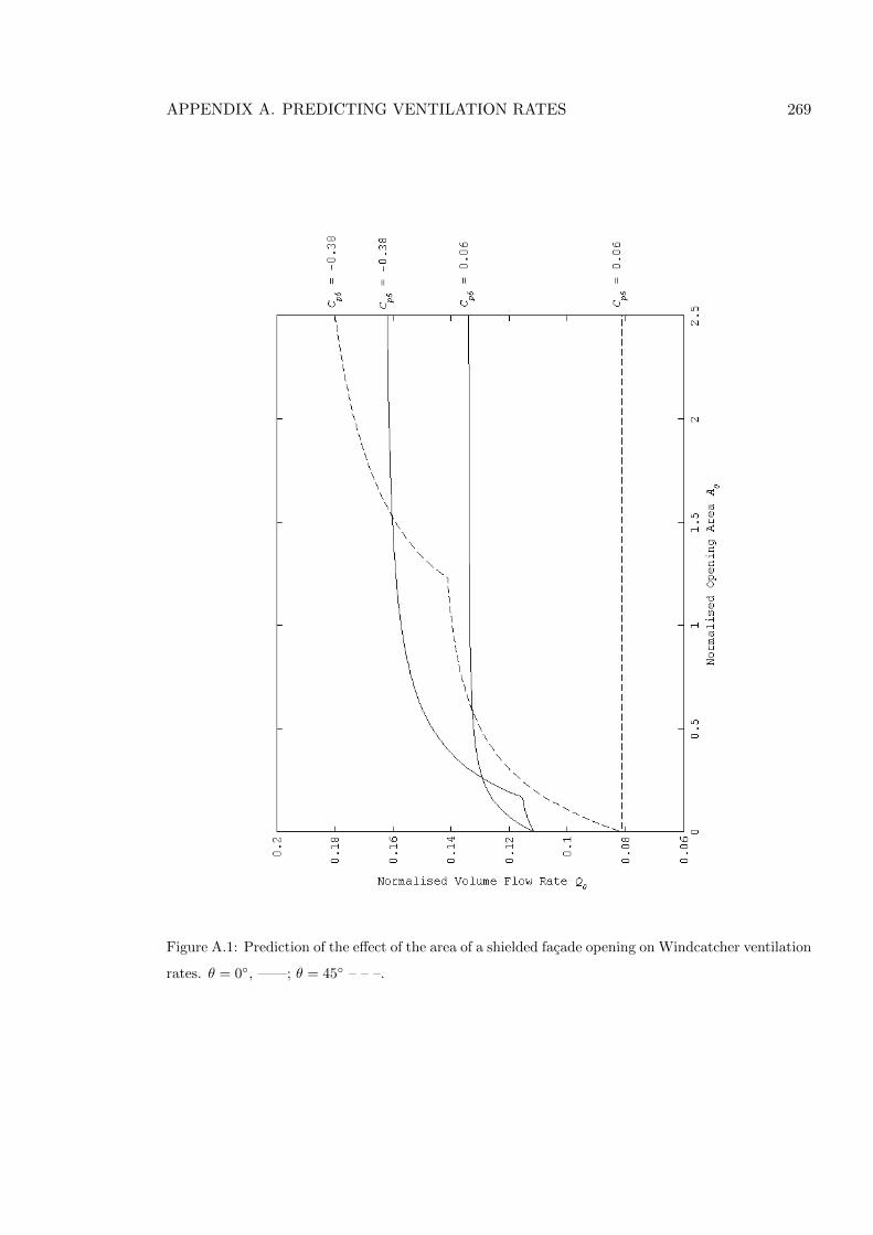
APPENDIX A. PREDICTING VENTILATION RATES 269
Figure A.1: Prediction of the effect of the area of a shielded facade opening on Windcatcher ventilation
rates. θ = 0◦, ——; θ = 45◦ – – –.
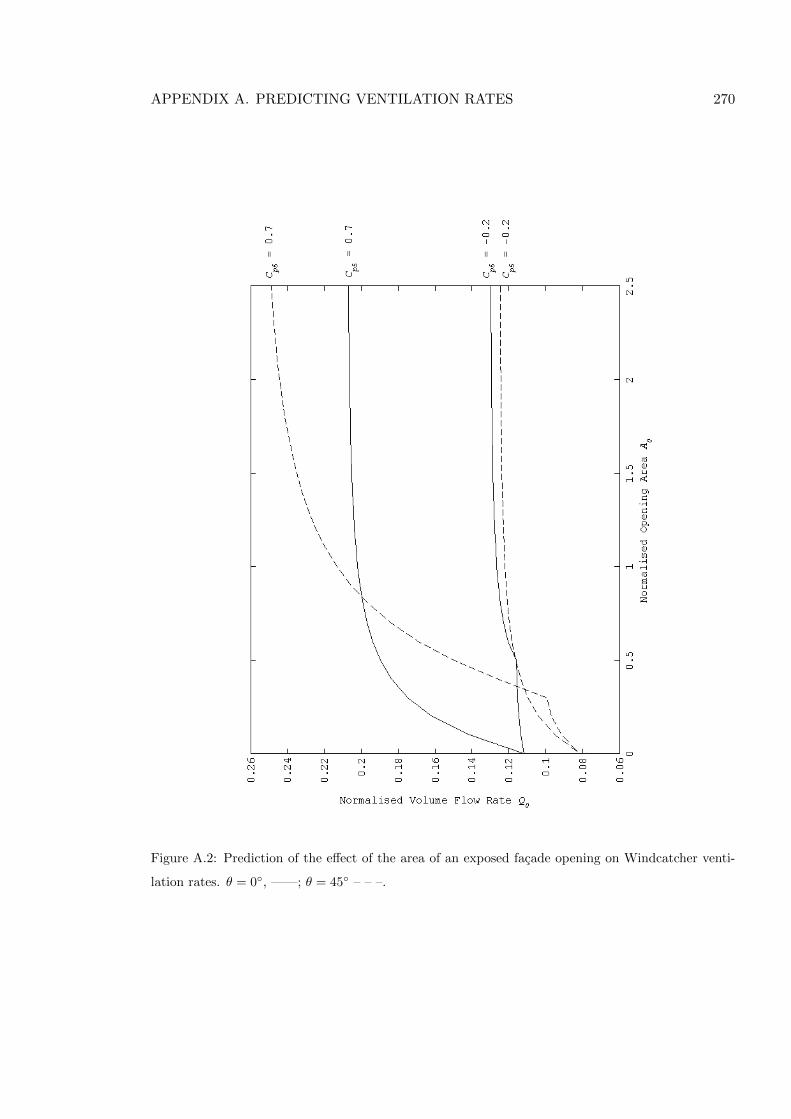
APPENDIX A. PREDICTING VENTILATION RATES 270
Figure A.2: Prediction of the effect of the area of an exposed facade opening on Windcatcher venti-
lation rates. θ = 0◦, ——; θ = 45◦ – – –.
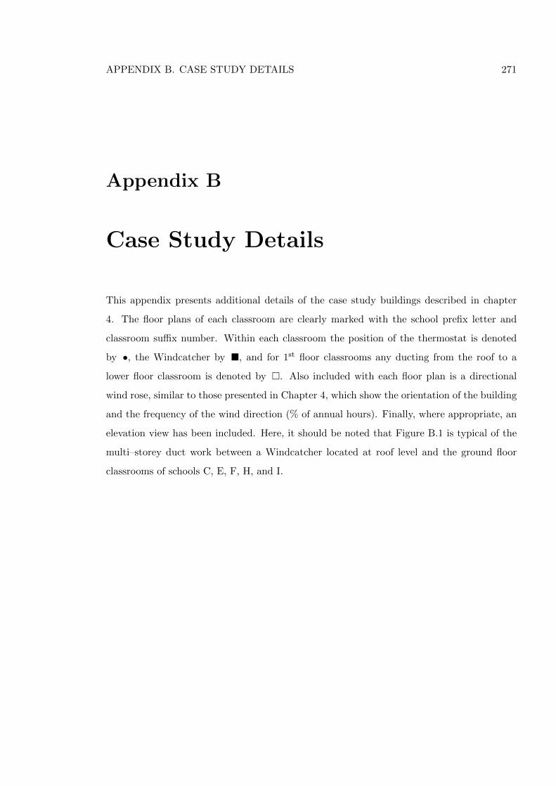
APPENDIX B. CASE STUDY DETAILS 271
Appendix B
Case Study Details
This appendix presents additional details of the case study buildings described in chapter
4. The floor plans of each classroom are clearly marked with the school prefix letter and
classroom suffix number. Within each classroom the position of the thermostat is denoted
by •, the Windcatcher by �, and for 1st floor classrooms any ducting from the roof to a
lower floor classroom is denoted by �. Also included with each floor plan is a directional
wind rose, similar to those presented in Chapter 4, which show the orientation of the building
and the frequency of the wind direction (% of annual hours). Finally, where appropriate, an
elevation view has been included. Here, it should be noted that Figure B.1 is typical of the
multi–storey duct work between a Windcatcher located at roof level and the ground floor
classrooms of schools C, E, F, H, and I.
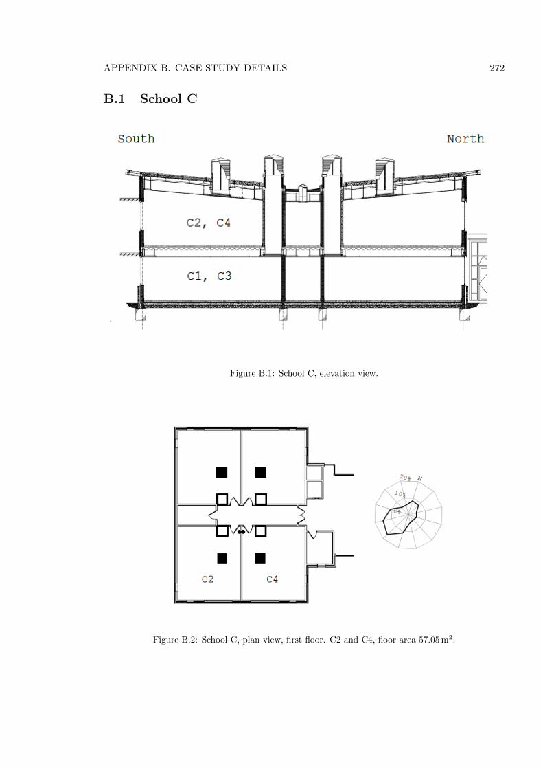
APPENDIX B. CASE STUDY DETAILS 272
B.1 School C
Figure B.1: School C, elevation view.
Figure B.2: School C, plan view, first floor. C2 and C4, floor area 57.05 m2.
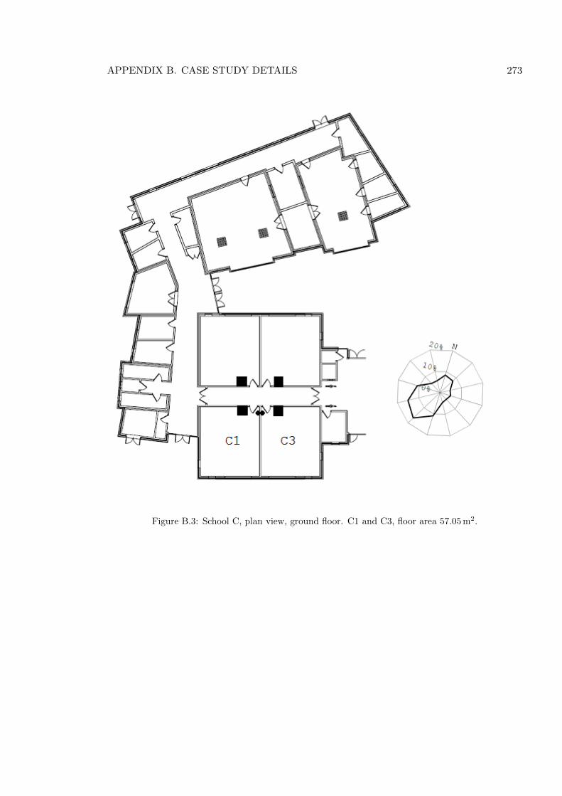
APPENDIX B. CASE STUDY DETAILS 273
Figure B.3: School C, plan view, ground floor. C1 and C3, floor area 57.05 m2.
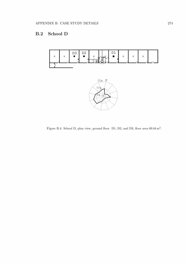
APPENDIX B. CASE STUDY DETAILS 274
B.2 School D
Figure B.4: School D, plan view, ground floor. D1, D2, and D3, floor area 69.84 m2.
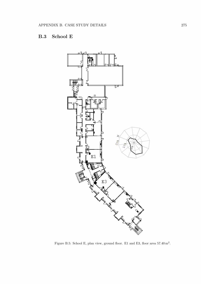
APPENDIX B. CASE STUDY DETAILS 275
B.3 School E
Figure B.5: School E, plan view, ground floor. E1 and E3, floor area 57.40 m2.
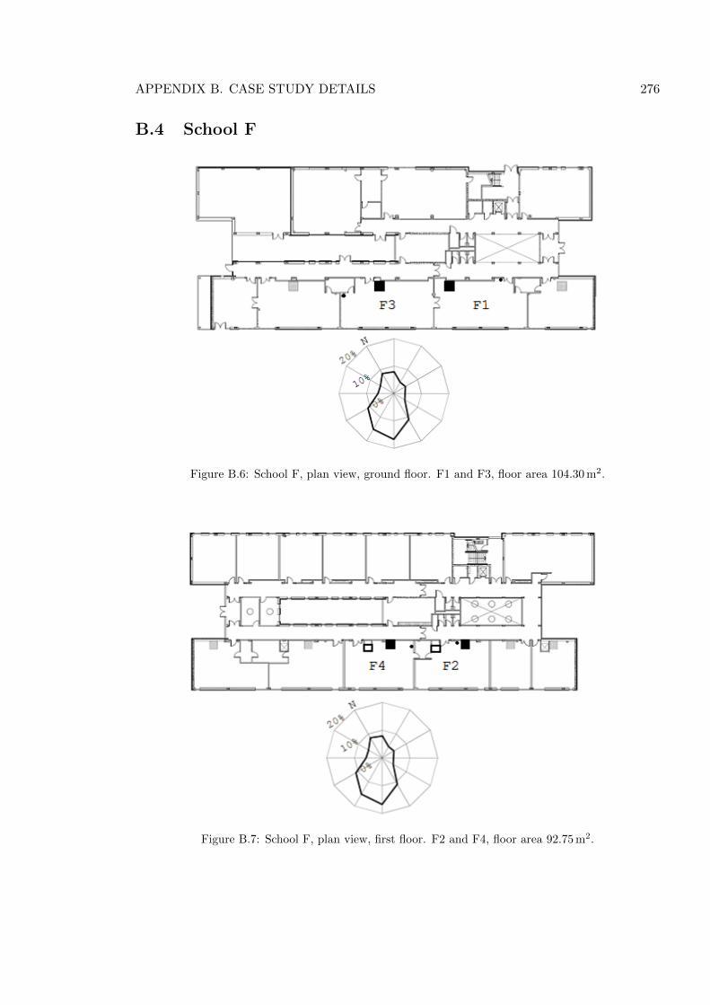
APPENDIX B. CASE STUDY DETAILS 276
B.4 School F
Figure B.6: School F, plan view, ground floor. F1 and F3, floor area 104.30 m2.
Figure B.7: School F, plan view, first floor. F2 and F4, floor area 92.75 m2.
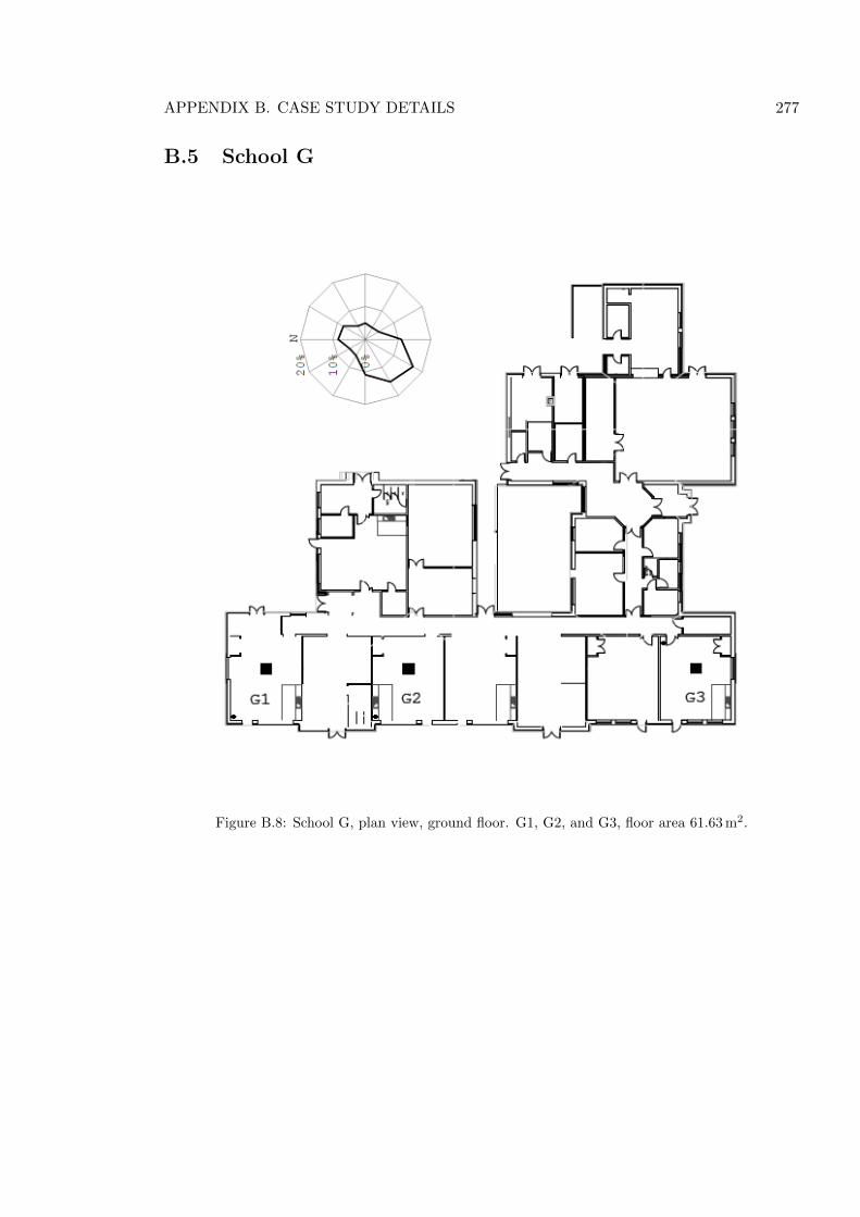
APPENDIX B. CASE STUDY DETAILS 277
B.5 School G
Figure B.8: School G, plan view, ground floor. G1, G2, and G3, floor area 61.63 m2.
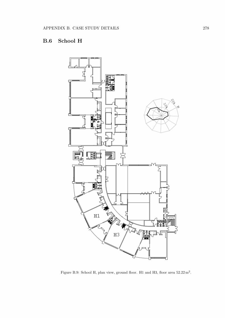
APPENDIX B. CASE STUDY DETAILS 278
B.6 School H
Figure B.9: School H, plan view, ground floor. H1 and H3, floor area 52.22 m2.
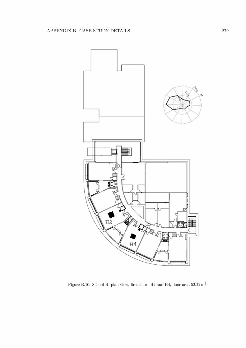
APPENDIX B. CASE STUDY DETAILS 279
Figure B.10: School H, plan view, first floor. H2 and H4, floor area 52.22 m2.
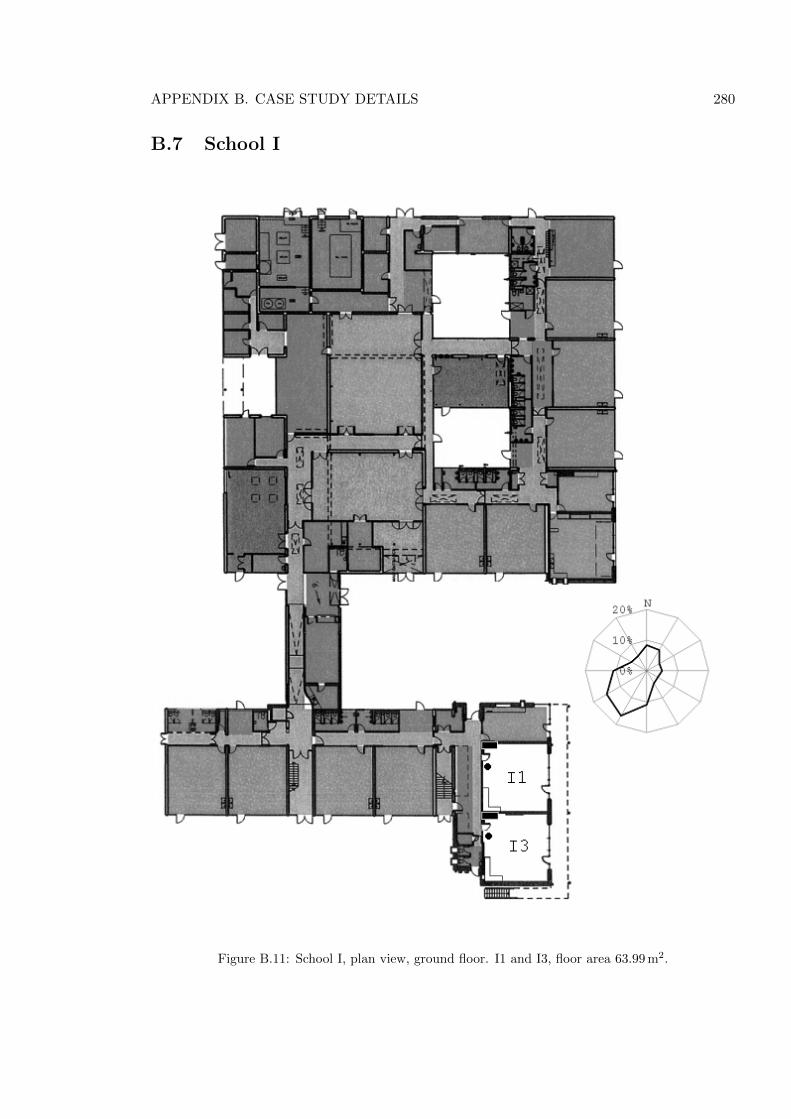
APPENDIX B. CASE STUDY DETAILS 280
B.7 School I
Figure B.11: School I, plan view, ground floor. I1 and I3, floor area 63.99 m2.
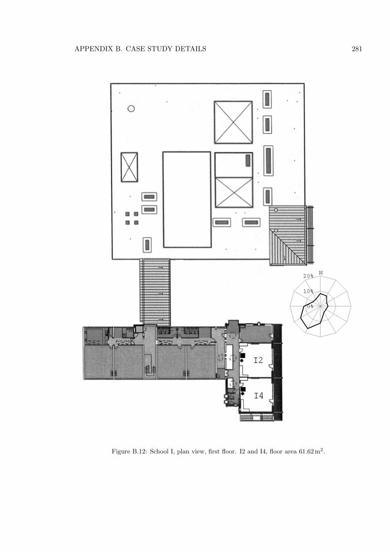
APPENDIX B. CASE STUDY DETAILS 281
Figure B.12: School I, plan view, first floor. I2 and I4, floor area 61.62 m2.
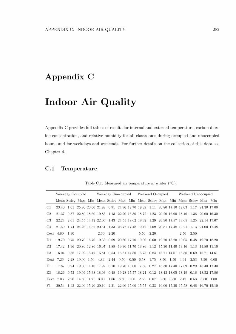
APPENDIX C. INDOOR AIR QUALITY 282
Appendix C
Indoor Air Quality
Appendix C provides full tables of results for internal and external temperature, carbon diox-
ide concentration, and relative humidity for all classrooms during occupied and unoccupied
hours, and for weekdays and weekends. For further details on the collection of this data see
Chapter 4.
C.1 Temperature
Table C.1: Measured air temperature in winter (◦C).
Weekday Occupied Weekday Unoccupied Weekend Occupied Weekend Unoccupied
Mean Stdev Max Min Mean Stdev Max Min Mean Stdev Max Min Mean Stdev Max Min
C1 23.40 1.01 25.90 20.60 21.99 0.91 24.90 19.70 19.32 1.11 20.80 17.10 19.03 1.17 21.30 17.00
C2 21.37 0.87 22.80 18.60 19.85 1.13 22.20 16.30 18.72 1.23 20.20 16.90 18.46 1.36 20.60 16.30
C3 22.24 2.01 24.55 14.42 22.06 1.43 24.55 18.62 19.32 1.29 20.90 17.57 19.65 1.25 22.14 17.67
C4 21.59 1.74 24.26 14.52 20.51 1.33 23.77 17.48 19.42 1.09 20.81 17.48 19.21 1.13 21.00 17.48
Cext 4.80 1.90 2.30 2.20 5.50 2.20 2.50 2.50
D1 19.70 0.75 20.70 16.70 19.33 0.69 20.60 17.70 19.00 0.60 19.70 18.20 19.05 0.48 19.70 18.20
D2 17.42 1.96 20.80 12.80 16.07 1.88 19.30 11.70 13.86 1.12 15.30 11.40 13.16 1.13 14.80 11.10
D3 16.04 0.38 17.09 15.47 15.81 0.54 16.81 14.80 15.75 0.84 16.71 14.61 15.80 0.69 16.71 14.61
Dext 7.26 2.28 19.00 1.50 4.84 2.44 9.50 -0.50 6.58 1.75 8.50 1.50 4.91 2.53 7.50 0.00
E1 17.87 0.94 19.30 14.10 17.92 0.70 19.70 15.00 17.86 0.27 18.30 17.40 17.69 0.29 18.40 17.30
E3 18.26 0.53 19.09 15.38 18.03 0.48 19.28 15.57 18.21 0.12 18.43 18.05 18.19 0.16 18.52 17.86
Eext 7.03 2.96 14.50 0.50 3.00 1.66 8.50 0.00 2.63 0.67 3.50 0.50 2.42 0.53 3.50 1.00
F1 20.54 1.93 22.90 15.20 20.10 2.21 22.90 15.00 15.57 0.33 16.00 15.20 15.58 0.46 16.70 15.10
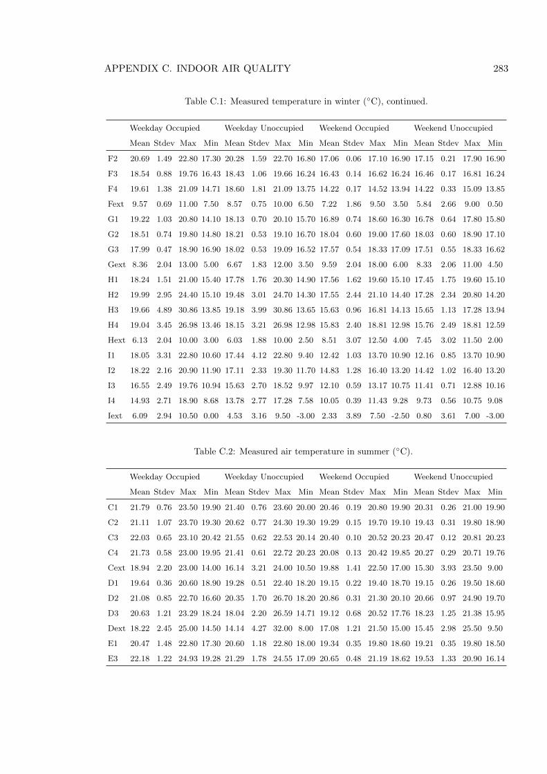
APPENDIX C. INDOOR AIR QUALITY 283
Table C.1: Measured temperature in winter (◦C), continued.
Weekday Occupied Weekday Unoccupied Weekend Occupied Weekend Unoccupied
Mean Stdev Max Min Mean Stdev Max Min Mean Stdev Max Min Mean Stdev Max Min
F2 20.69 1.49 22.80 17.30 20.28 1.59 22.70 16.80 17.06 0.06 17.10 16.90 17.15 0.21 17.90 16.90
F3 18.54 0.88 19.76 16.43 18.43 1.06 19.66 16.24 16.43 0.14 16.62 16.24 16.46 0.17 16.81 16.24
F4 19.61 1.38 21.09 14.71 18.60 1.81 21.09 13.75 14.22 0.17 14.52 13.94 14.22 0.33 15.09 13.85
Fext 9.57 0.69 11.00 7.50 8.57 0.75 10.00 6.50 7.22 1.86 9.50 3.50 5.84 2.66 9.00 0.50
G1 19.22 1.03 20.80 14.10 18.13 0.70 20.10 15.70 16.89 0.74 18.60 16.30 16.78 0.64 17.80 15.80
G2 18.51 0.74 19.80 14.80 18.21 0.53 19.10 16.70 18.04 0.60 19.00 17.60 18.03 0.60 18.90 17.10
G3 17.99 0.47 18.90 16.90 18.02 0.53 19.09 16.52 17.57 0.54 18.33 17.09 17.51 0.55 18.33 16.62
Gext 8.36 2.04 13.00 5.00 6.67 1.83 12.00 3.50 9.59 2.04 18.00 6.00 8.33 2.06 11.00 4.50
H1 18.24 1.51 21.00 15.40 17.78 1.76 20.30 14.90 17.56 1.62 19.60 15.10 17.45 1.75 19.60 15.10
H2 19.99 2.95 24.40 15.10 19.48 3.01 24.70 14.30 17.55 2.44 21.10 14.40 17.28 2.34 20.80 14.20
H3 19.66 4.89 30.86 13.85 19.18 3.99 30.86 13.65 15.63 0.96 16.81 14.13 15.65 1.13 17.28 13.94
H4 19.04 3.45 26.98 13.46 18.15 3.21 26.98 12.98 15.83 2.40 18.81 12.98 15.76 2.49 18.81 12.59
Hext 6.13 2.04 10.00 3.00 6.03 1.88 10.00 2.50 8.51 3.07 12.50 4.00 7.45 3.02 11.50 2.00
I1 18.05 3.31 22.80 10.60 17.44 4.12 22.80 9.40 12.42 1.03 13.70 10.90 12.16 0.85 13.70 10.90
I2 18.22 2.16 20.90 11.90 17.11 2.33 19.30 11.70 14.83 1.28 16.40 13.20 14.42 1.02 16.40 13.20
I3 16.55 2.49 19.76 10.94 15.63 2.70 18.52 9.97 12.10 0.59 13.17 10.75 11.41 0.71 12.88 10.16
I4 14.93 2.71 18.90 8.68 13.78 2.77 17.28 7.58 10.05 0.39 11.43 9.28 9.73 0.56 10.75 9.08
Iext 6.09 2.94 10.50 0.00 4.53 3.16 9.50 -3.00 2.33 3.89 7.50 -2.50 0.80 3.61 7.00 -3.00
Table C.2: Measured air temperature in summer (◦C).
Weekday Occupied Weekday Unoccupied Weekend Occupied Weekend Unoccupied
Mean Stdev Max Min Mean Stdev Max Min Mean Stdev Max Min Mean Stdev Max Min
C1 21.79 0.76 23.50 19.90 21.40 0.76 23.60 20.00 20.46 0.19 20.80 19.90 20.31 0.26 21.00 19.90
C2 21.11 1.07 23.70 19.30 20.62 0.77 24.30 19.30 19.29 0.15 19.70 19.10 19.43 0.31 19.80 18.90
C3 22.03 0.65 23.10 20.42 21.55 0.62 22.53 20.14 20.40 0.10 20.52 20.23 20.47 0.12 20.81 20.23
C4 21.73 0.58 23.00 19.95 21.41 0.61 22.72 20.23 20.08 0.13 20.42 19.85 20.27 0.29 20.71 19.76
Cext 18.94 2.20 23.00 14.00 16.14 3.21 24.00 10.50 19.88 1.41 22.50 17.00 15.30 3.93 23.50 9.00
D1 19.64 0.36 20.60 18.90 19.28 0.51 22.40 18.20 19.15 0.22 19.40 18.70 19.15 0.26 19.50 18.60
D2 21.08 0.85 22.70 16.60 20.35 1.70 26.70 18.20 20.86 0.31 21.30 20.10 20.66 0.97 24.90 19.70
D3 20.63 1.21 23.29 18.24 18.04 2.20 26.59 14.71 19.12 0.68 20.52 17.76 18.23 1.25 21.38 15.95
Dext 18.22 2.45 25.00 14.50 14.14 4.27 32.00 8.00 17.08 1.21 21.50 15.00 15.45 2.98 25.50 9.50
E1 20.47 1.48 22.80 17.30 20.60 1.18 22.80 18.00 19.34 0.35 19.80 18.60 19.21 0.35 19.80 18.50
E3 22.18 1.22 24.93 19.28 21.29 1.78 24.55 17.09 20.65 0.48 21.19 18.62 19.53 1.33 20.90 16.14
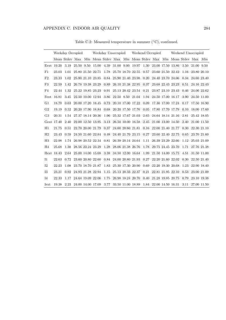
APPENDIX C. INDOOR AIR QUALITY 284
Table C.2: Measured temperature in summer (◦C), continued.
Weekday Occupied Weekday Unoccupied Weekend Occupied Weekend Unoccupied
Mean Stdev Max Min Mean Stdev Max Min Mean Stdev Max Min Mean Stdev Max Min
Eext 19.20 3.19 25.50 9.50 15.00 4.39 31.00 9.00 19.97 1.30 23.00 17.50 13.86 3.50 21.00 9.50
F1 23.03 1.01 25.80 21.50 22.71 1.78 25.70 18.70 22.55 0.57 23.60 21.50 22.42 1.16 23.80 20.10
F2 23.33 1.02 25.90 21.10 23.85 0.84 25.90 21.40 23.98 0.20 24.40 23.70 24.06 0.34 24.60 23.40
F3 22.59 1.42 26.78 19.38 23.29 0.89 26.10 21.38 22.95 0.37 23.68 22.43 23.23 0.51 24.16 22.43
F4 22.44 1.32 25.22 19.85 23.23 0.91 25.13 20.42 23.54 0.21 23.87 23.10 23.43 0.46 24.06 22.62
Fext 16.81 3.45 22.50 10.00 12.94 3.86 22.50 8.50 21.04 1.94 24.50 17.00 16.17 3.90 24.50 11.00
G1 18.70 0.63 20.00 17.20 18.45 0.73 20.10 17.00 17.22 0.09 17.30 17.00 17.24 0.17 17.50 16.90
G2 19.19 0.52 20.20 17.90 18.84 0.68 20.20 17.50 17.76 0.05 17.80 17.70 17.79 0.10 18.00 17.60
G3 20.31 1.54 27.37 18.14 20.36 1.96 25.32 17.67 21.03 2.65 24.64 18.14 21.16 2.81 25.42 18.05
Gext 17.40 2.40 22.00 12.50 13.95 3.13 26.50 10.00 16.58 2.45 21.00 13.00 14.50 2.40 21.00 11.50
H1 21.75 0.51 22.70 20.00 21.79 0.37 24.60 20.60 21.81 0.16 22.00 21.40 21.77 0.30 22.30 21.10
H2 23.43 0.59 24.50 21.60 22.84 0.48 24.40 21.70 23.15 0.27 23.60 22.40 22.75 0.65 23.70 21.60
H3 22.98 1.74 26.98 20.52 22.34 0.81 26.39 20.14 24.64 1.11 26.39 23.29 22.66 1.12 25.03 21.09
H4 25.68 1.38 28.56 22.24 23.29 1.28 28.06 21.38 26.76 1.78 29.75 24.45 23.70 1.71 27.76 21.38
Hext 18.43 2.64 25.00 14.00 15.68 3.38 34.50 12.00 16.64 1.99 21.50 14.00 15.75 4.51 31.50 11.00
I1 22.63 0.72 23.60 20.80 22.60 0.84 24.00 20.80 21.93 0.27 22.20 21.60 22.02 0.30 22.50 21.40
I2 22.23 1.08 23.70 18.70 21.87 1.83 25.30 17.30 20.90 0.69 22.20 19.30 20.68 1.23 22.90 18.40
I3 23.21 0.92 24.93 21.28 22.94 1.15 25.13 20.33 22.37 0.21 22.81 21.95 22.10 0.53 23.00 21.09
I4 22.33 1.17 24.64 19.09 22.06 1.75 26.98 18.24 20.70 0.40 21.28 19.85 20.75 0.79 23.10 19.38
Iext 19.38 2.23 24.00 14.00 17.09 3.77 33.50 11.00 18.89 1.84 22.00 14.50 16.31 3.11 27.00 11.50
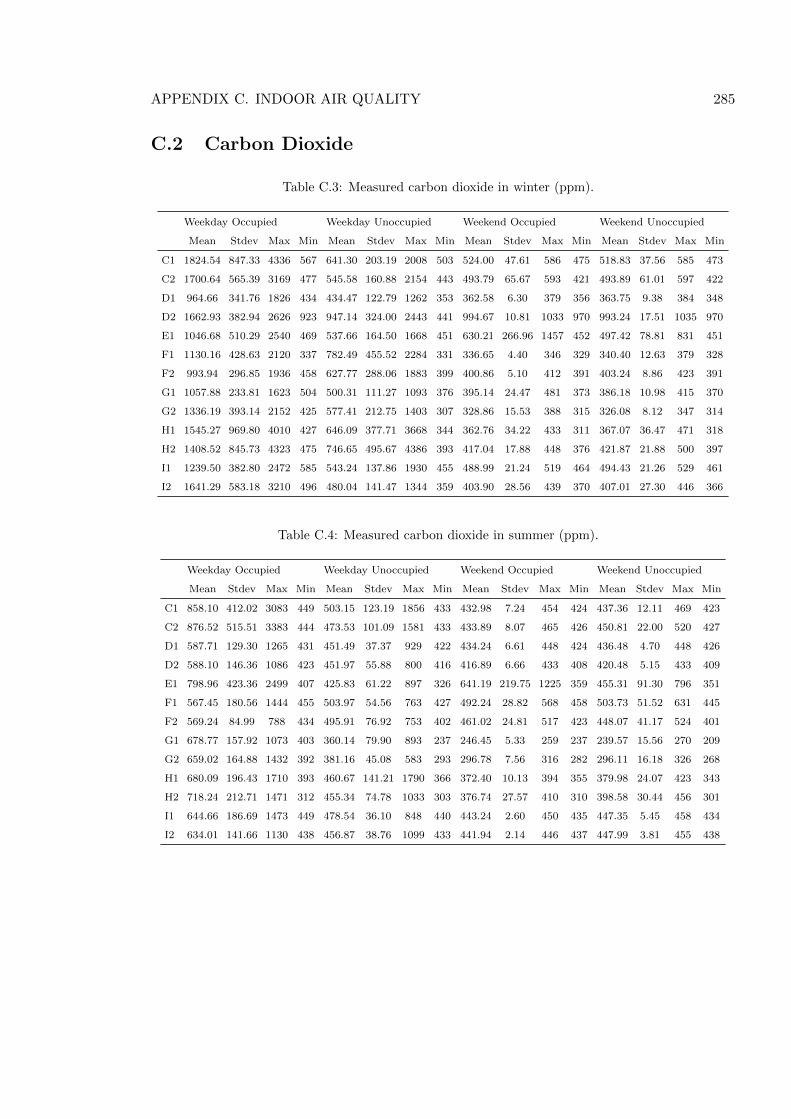
APPENDIX C. INDOOR AIR QUALITY 285
C.2 Carbon Dioxide
Table C.3: Measured carbon dioxide in winter (ppm).
Weekday Occupied Weekday Unoccupied Weekend Occupied Weekend Unoccupied
Mean Stdev Max Min Mean Stdev Max Min Mean Stdev Max Min Mean Stdev Max Min
C1 1824.54 847.33 4336 567 641.30 203.19 2008 503 524.00 47.61 586 475 518.83 37.56 585 473
C2 1700.64 565.39 3169 477 545.58 160.88 2154 443 493.79 65.67 593 421 493.89 61.01 597 422
D1 964.66 341.76 1826 434 434.47 122.79 1262 353 362.58 6.30 379 356 363.75 9.38 384 348
D2 1662.93 382.94 2626 923 947.14 324.00 2443 441 994.67 10.81 1033 970 993.24 17.51 1035 970
E1 1046.68 510.29 2540 469 537.66 164.50 1668 451 630.21 266.96 1457 452 497.42 78.81 831 451
F1 1130.16 428.63 2120 337 782.49 455.52 2284 331 336.65 4.40 346 329 340.40 12.63 379 328
F2 993.94 296.85 1936 458 627.77 288.06 1883 399 400.86 5.10 412 391 403.24 8.86 423 391
G1 1057.88 233.81 1623 504 500.31 111.27 1093 376 395.14 24.47 481 373 386.18 10.98 415 370
G2 1336.19 393.14 2152 425 577.41 212.75 1403 307 328.86 15.53 388 315 326.08 8.12 347 314
H1 1545.27 969.80 4010 427 646.09 377.71 3668 344 362.76 34.22 433 311 367.07 36.47 471 318
H2 1408.52 845.73 4323 475 746.65 495.67 4386 393 417.04 17.88 448 376 421.87 21.88 500 397
I1 1239.50 382.80 2472 585 543.24 137.86 1930 455 488.99 21.24 519 464 494.43 21.26 529 461
I2 1641.29 583.18 3210 496 480.04 141.47 1344 359 403.90 28.56 439 370 407.01 27.30 446 366
Table C.4: Measured carbon dioxide in summer (ppm).
Weekday Occupied Weekday Unoccupied Weekend Occupied Weekend Unoccupied
Mean Stdev Max Min Mean Stdev Max Min Mean Stdev Max Min Mean Stdev Max Min
C1 858.10 412.02 3083 449 503.15 123.19 1856 433 432.98 7.24 454 424 437.36 12.11 469 423
C2 876.52 515.51 3383 444 473.53 101.09 1581 433 433.89 8.07 465 426 450.81 22.00 520 427
D1 587.71 129.30 1265 431 451.49 37.37 929 422 434.24 6.61 448 424 436.48 4.70 448 426
D2 588.10 146.36 1086 423 451.97 55.88 800 416 416.89 6.66 433 408 420.48 5.15 433 409
E1 798.96 423.36 2499 407 425.83 61.22 897 326 641.19 219.75 1225 359 455.31 91.30 796 351
F1 567.45 180.56 1444 455 503.97 54.56 763 427 492.24 28.82 568 458 503.73 51.52 631 445
F2 569.24 84.99 788 434 495.91 76.92 753 402 461.02 24.81 517 423 448.07 41.17 524 401
G1 678.77 157.92 1073 403 360.14 79.90 893 237 246.45 5.33 259 237 239.57 15.56 270 209
G2 659.02 164.88 1432 392 381.16 45.08 583 293 296.78 7.56 316 282 296.11 16.18 326 268
H1 680.09 196.43 1710 393 460.67 141.21 1790 366 372.40 10.13 394 355 379.98 24.07 423 343
H2 718.24 212.71 1471 312 455.34 74.78 1033 303 376.74 27.57 410 310 398.58 30.44 456 301
I1 644.66 186.69 1473 449 478.54 36.10 848 440 443.24 2.60 450 435 447.35 5.45 458 434
I2 634.01 141.66 1130 438 456.87 38.76 1099 433 441.94 2.14 446 437 447.99 3.81 455 438
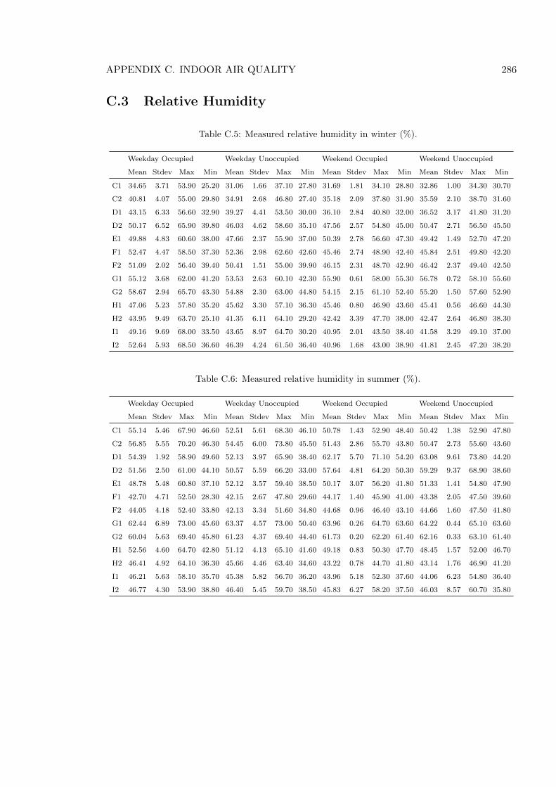
APPENDIX C. INDOOR AIR QUALITY 286
C.3 Relative Humidity
Table C.5: Measured relative humidity in winter (%).
Weekday Occupied Weekday Unoccupied Weekend Occupied Weekend Unoccupied
Mean Stdev Max Min Mean Stdev Max Min Mean Stdev Max Min Mean Stdev Max Min
C1 34.65 3.71 53.90 25.20 31.06 1.66 37.10 27.80 31.69 1.81 34.10 28.80 32.86 1.00 34.30 30.70
C2 40.81 4.07 55.00 29.80 34.91 2.68 46.80 27.40 35.18 2.09 37.80 31.90 35.59 2.10 38.70 31.60
D1 43.15 6.33 56.60 32.90 39.27 4.41 53.50 30.00 36.10 2.84 40.80 32.00 36.52 3.17 41.80 31.20
D2 50.17 6.52 65.90 39.80 46.03 4.62 58.60 35.10 47.56 2.57 54.80 45.00 50.47 2.71 56.50 45.50
E1 49.88 4.83 60.60 38.00 47.66 2.37 55.90 37.00 50.39 2.78 56.60 47.30 49.42 1.49 52.70 47.20
F1 52.47 4.47 58.50 37.30 52.36 2.98 62.60 42.60 45.46 2.74 48.90 42.40 45.84 2.51 49.80 42.20
F2 51.09 2.02 56.40 39.40 50.41 1.51 55.00 39.90 46.15 2.31 48.70 42.90 46.42 2.37 49.40 42.50
G1 55.12 3.68 62.00 41.20 53.53 2.63 60.10 42.30 55.90 0.61 58.00 55.30 56.78 0.72 58.10 55.60
G2 58.67 2.94 65.70 43.30 54.88 2.30 63.00 44.80 54.15 2.15 61.10 52.40 55.20 1.50 57.60 52.90
H1 47.06 5.23 57.80 35.20 45.62 3.30 57.10 36.30 45.46 0.80 46.90 43.60 45.41 0.56 46.60 44.30
H2 43.95 9.49 63.70 25.10 41.35 6.11 64.10 29.20 42.42 3.39 47.70 38.00 42.47 2.64 46.80 38.30
I1 49.16 9.69 68.00 33.50 43.65 8.97 64.70 30.20 40.95 2.01 43.50 38.40 41.58 3.29 49.10 37.00
I2 52.64 5.93 68.50 36.60 46.39 4.24 61.50 36.40 40.96 1.68 43.00 38.90 41.81 2.45 47.20 38.20
Table C.6: Measured relative humidity in summer (%).
Weekday Occupied Weekday Unoccupied Weekend Occupied Weekend Unoccupied
Mean Stdev Max Min Mean Stdev Max Min Mean Stdev Max Min Mean Stdev Max Min
C1 55.14 5.46 67.90 46.60 52.51 5.61 68.30 46.10 50.78 1.43 52.90 48.40 50.42 1.38 52.90 47.80
C2 56.85 5.55 70.20 46.30 54.45 6.00 73.80 45.50 51.43 2.86 55.70 43.80 50.47 2.73 55.60 43.60
D1 54.39 1.92 58.90 49.60 52.13 3.97 65.90 38.40 62.17 5.70 71.10 54.20 63.08 9.61 73.80 44.20
D2 51.56 2.50 61.00 44.10 50.57 5.59 66.20 33.00 57.64 4.81 64.20 50.30 59.29 9.37 68.90 38.60
E1 48.78 5.48 60.80 37.10 52.12 3.57 59.40 38.50 50.17 3.07 56.20 41.80 51.33 1.41 54.80 47.90
F1 42.70 4.71 52.50 28.30 42.15 2.67 47.80 29.60 44.17 1.40 45.90 41.00 43.38 2.05 47.50 39.60
F2 44.05 4.18 52.40 33.80 42.13 3.34 51.60 34.80 44.68 0.96 46.40 43.10 44.66 1.60 47.50 41.80
G1 62.44 6.89 73.00 45.60 63.37 4.57 73.00 50.40 63.96 0.26 64.70 63.60 64.22 0.44 65.10 63.60
G2 60.04 5.63 69.40 45.80 61.23 4.37 69.40 44.40 61.73 0.20 62.20 61.40 62.16 0.33 63.10 61.40
H1 52.56 4.60 64.70 42.80 51.12 4.13 65.10 41.60 49.18 0.83 50.30 47.70 48.45 1.57 52.00 46.70
H2 46.41 4.92 64.10 36.30 45.66 4.46 63.40 34.60 43.22 0.78 44.70 41.80 43.14 1.76 46.90 41.20
I1 46.21 5.63 58.10 35.70 45.38 5.82 56.70 36.20 43.96 5.18 52.30 37.60 44.06 6.23 54.80 36.40
I2 46.77 4.30 53.90 38.80 46.40 5.45 59.70 38.50 45.83 6.27 58.20 37.50 46.03 8.57 60.70 35.80
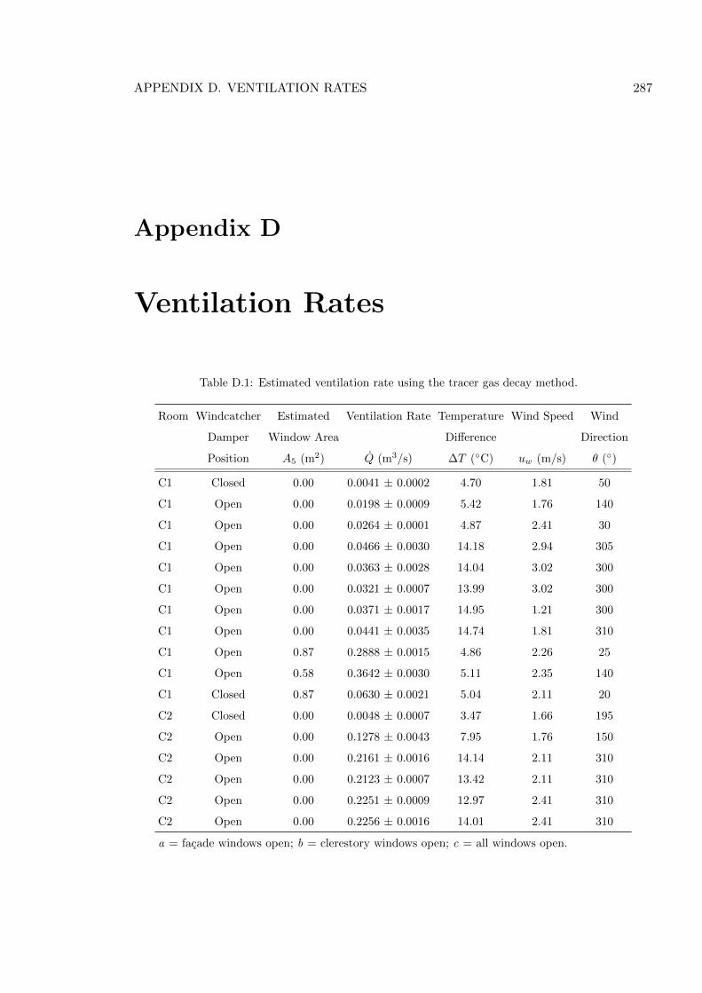
APPENDIX D. VENTILATION RATES 287
Appendix D
Ventilation Rates
Table D.1: Estimated ventilation rate using the tracer gas decay method.
Room Windcatcher Estimated Ventilation Rate Temperature Wind Speed Wind
Damper Window Area Difference Direction
Position A5 (m2) Q (m3/s) ∆T (◦C) uw (m/s) θ (◦)
C1 Closed 0.00 0.0041 ± 0.0002 4.70 1.81 50
C1 Open 0.00 0.0198 ± 0.0009 5.42 1.76 140
C1 Open 0.00 0.0264 ± 0.0001 4.87 2.41 30
C1 Open 0.00 0.0466 ± 0.0030 14.18 2.94 305
C1 Open 0.00 0.0363 ± 0.0028 14.04 3.02 300
C1 Open 0.00 0.0321 ± 0.0007 13.99 3.02 300
C1 Open 0.00 0.0371 ± 0.0017 14.95 1.21 300
C1 Open 0.00 0.0441 ± 0.0035 14.74 1.81 310
C1 Open 0.87 0.2888 ± 0.0015 4.86 2.26 25
C1 Open 0.58 0.3642 ± 0.0030 5.11 2.35 140
C1 Closed 0.87 0.0630 ± 0.0021 5.04 2.11 20
C2 Closed 0.00 0.0048 ± 0.0007 3.47 1.66 195
C2 Open 0.00 0.1278 ± 0.0043 7.95 1.76 150
C2 Open 0.00 0.2161 ± 0.0016 14.14 2.11 310
C2 Open 0.00 0.2123 ± 0.0007 13.42 2.11 310
C2 Open 0.00 0.2251 ± 0.0009 12.97 2.41 310
C2 Open 0.00 0.2256 ± 0.0016 14.01 2.41 310
a = facade windows open; b = clerestory windows open; c = all windows open.
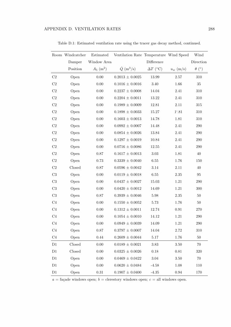
APPENDIX D. VENTILATION RATES 288
Table D.1: Estimated ventilation rate using the tracer gas decay method, continued.
Room Windcatcher Estimated Ventilation Rate Temperature Wind Speed Wind
Damper Window Area Difference Direction
Position A5 (m2) Q (m3/s) ∆T (◦C) uw (m/s) θ (◦)
C2 Open 0.00 0.2013 ± 0.0025 13.99 2.57 310
C2 Open 0.00 0.1016 ± 0.0016 3.40 1.66 35
C2 Open 0.00 0.2237 ± 0.0008 14.04 2.41 310
C2 Open 0.00 0.2204 ± 0.0011 13.22 2.41 310
C2 Open 0.00 0.1989 ± 0.0009 12.81 2.11 315
C2 Open 0.00 0.1898 ± 0.0033 15.27 1‘.81 310
C2 Open 0.00 0.1603 ± 0.0013 14.78 1.81 310
C2 Open 0.00 0.0992 ± 0.0007 14.48 2.41 290
C2 Open 0.00 0.0854 ± 0.0026 13.84 2.41 290
C2 Open 0.00 0.1297 ± 0.0019 10.84 2.41 290
C2 Open 0.00 0.0716 ± 0.0086 12.55 2.41 290
C2 Open 0.87 0.1617 ± 0.0013 3.03 1.81 40
C2 Open 0.73 0.3339 ± 0.0040 6.55 1.76 150
C2 Closed 0.87 0.0596 ± 0.0042 3.14 2.11 40
C3 Open 0.00 0.0119 ± 0.0018 6.55 2.35 95
C3 Open 0.00 0.0437 ± 0.0027 15.03 1.21 290
C3 Open 0.00 0.0420 ± 0.0012 14.69 1.21 300
C3 Open 0.87 0.3939 ± 0.0046 5.98 2.35 50
C4 Open 0.00 0.1550 ± 0.0052 5.73 1.76 50
C4 Open 0.00 0.1312 ± 0.0011 12.74 0.91 270
C4 Open 0.00 0.1054 ± 0.0010 14.12 1.21 290
C4 Open 0.00 0.0949 ± 0.0039 14.09 1.21 290
C4 Open 0.87 0.3797 ± 0.0007 14.04 2.72 310
C4 Open 0.44 0.2609 ± 0.0044 5.17 1.76 50
D1 Closed 0.00 0.0189 ± 0.0021 3.83 3.50 70
D1 Closed 0.00 0.0325 ± 0.0026 0.18 0.81 320
D1 Open 0.00 0.0469 ± 0.0422 3.04 3.50 70
D1 Open 0.00 0.0620 ± 0.0484 -4.58 1.08 110
D1 Open 0.31 0.1907 ± 0.0400 -4.35 0.94 170
a = facade windows open; b = clerestory windows open; c = all windows open.
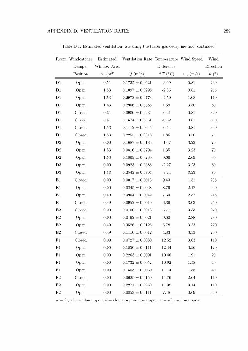
APPENDIX D. VENTILATION RATES 289
Table D.1: Estimated ventilation rate using the tracer gas decay method, continued.
Room Windcatcher Estimated Ventilation Rate Temperature Wind Speed Wind
Damper Window Area Difference Direction
Position A5 (m2) Q (m3/s) ∆T (◦C) uw (m/s) θ (◦)
D1 Open 0.51 0.1725 ± 0.0621 -3.69 0.81 230
D1 Open 1.53 0.1097 ± 0.0296 -2.85 0.81 265
D1 Open 1.53 0.2973 ± 0.0773 -4.50 1.08 110
D1 Open 1.53 0.2966 ± 0.0386 1.59 3.50 80
D1 Closed 0.31 0.0900 ± 0.0234 -0.21 0.81 320
D1 Closed 0.51 0.1574 ± 0.0551 -0.32 0.81 300
D1 Closed 1.53 0.1112 ± 0.0645 -0.44 0.81 300
D1 Closed 1.53 0.2255 ± 0.0316 1.86 3.50 75
D2 Open 0.00 0.1687 ± 0.0186 -1.67 3.23 70
D2 Open 1.53 0.0810 ± 0.0704 1.35 3.23 70
D2 Open 1.53 0.1869 ± 0.0280 0.66 2.69 80
D3 Open 0.00 0.0923 ± 0.0388 -2.27 3.23 80
D3 Open 1.53 0.2542 ± 0.0305 -3.24 3.23 80
E1 Closed 0.00 0.0017 ± 0.0013 9.43 1.51 235
E1 Open 0.00 0.0245 ± 0.0028 8.79 2.12 240
E1 Open 0.49 0.3954 ± 0.0042 7.34 2.57 245
E1 Closed 0.49 0.0952 ± 0.0019 6.39 3.03 250
E2 Closed 0.00 0.0100 ± 0.0018 5.71 3.33 270
E2 Open 0.00 0.0192 ± 0.0021 9.62 2.88 280
E2 Open 0.49 0.3526 ± 0.0125 5.78 3.33 270
E2 Closed 0.49 0.1110 ± 0.0012 4.83 3.33 280
F1 Closed 0.00 0.0727 ± 0.0080 12.52 3.63 110
F1 Open 0.00 0.1850 ± 0.0111 12.44 3.96 120
F1 Open 0.00 0.2263 ± 0.0091 10.46 1.91 20
F1 Open 0.00 0.1732 ± 0.0052 10.92 1.58 40
F1 Open 0.00 0.1503 ± 0.0030 11.14 1.58 40
F2 Closed 0.00 0.0625 ± 0.0150 11.76 2.64 110
F2 Open 0.00 0.2271 ± 0.0250 11.38 3.14 110
F2 Open 0.00 0.0853 ± 0.0111 7.48 0.69 360
a = facade windows open; b = clerestory windows open; c = all windows open.
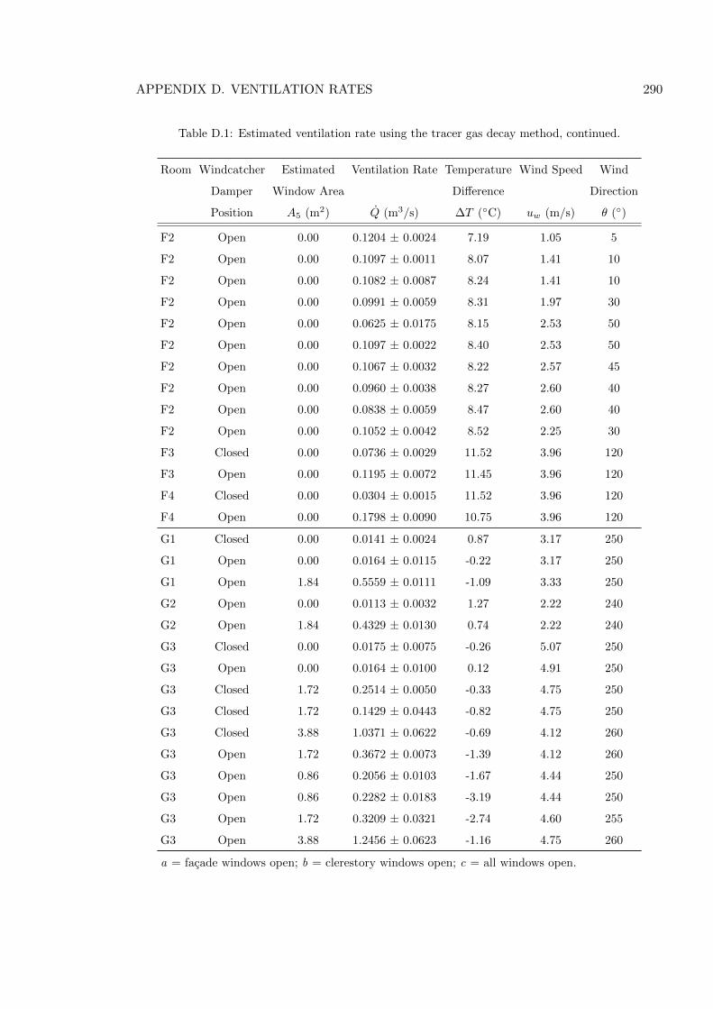
APPENDIX D. VENTILATION RATES 290
Table D.1: Estimated ventilation rate using the tracer gas decay method, continued.
Room Windcatcher Estimated Ventilation Rate Temperature Wind Speed Wind
Damper Window Area Difference Direction
Position A5 (m2) Q (m3/s) ∆T (◦C) uw (m/s) θ (◦)
F2 Open 0.00 0.1204 ± 0.0024 7.19 1.05 5
F2 Open 0.00 0.1097 ± 0.0011 8.07 1.41 10
F2 Open 0.00 0.1082 ± 0.0087 8.24 1.41 10
F2 Open 0.00 0.0991 ± 0.0059 8.31 1.97 30
F2 Open 0.00 0.0625 ± 0.0175 8.15 2.53 50
F2 Open 0.00 0.1097 ± 0.0022 8.40 2.53 50
F2 Open 0.00 0.1067 ± 0.0032 8.22 2.57 45
F2 Open 0.00 0.0960 ± 0.0038 8.27 2.60 40
F2 Open 0.00 0.0838 ± 0.0059 8.47 2.60 40
F2 Open 0.00 0.1052 ± 0.0042 8.52 2.25 30
F3 Closed 0.00 0.0736 ± 0.0029 11.52 3.96 120
F3 Open 0.00 0.1195 ± 0.0072 11.45 3.96 120
F4 Closed 0.00 0.0304 ± 0.0015 11.52 3.96 120
F4 Open 0.00 0.1798 ± 0.0090 10.75 3.96 120
G1 Closed 0.00 0.0141 ± 0.0024 0.87 3.17 250
G1 Open 0.00 0.0164 ± 0.0115 -0.22 3.17 250
G1 Open 1.84 0.5559 ± 0.0111 -1.09 3.33 250
G2 Open 0.00 0.0113 ± 0.0032 1.27 2.22 240
G2 Open 1.84 0.4329 ± 0.0130 0.74 2.22 240
G3 Closed 0.00 0.0175 ± 0.0075 -0.26 5.07 250
G3 Open 0.00 0.0164 ± 0.0100 0.12 4.91 250
G3 Closed 1.72 0.2514 ± 0.0050 -0.33 4.75 250
G3 Closed 1.72 0.1429 ± 0.0443 -0.82 4.75 250
G3 Closed 3.88 1.0371 ± 0.0622 -0.69 4.12 260
G3 Open 1.72 0.3672 ± 0.0073 -1.39 4.12 260
G3 Open 0.86 0.2056 ± 0.0103 -1.67 4.44 250
G3 Open 0.86 0.2282 ± 0.0183 -3.19 4.44 250
G3 Open 1.72 0.3209 ± 0.0321 -2.74 4.60 255
G3 Open 3.88 1.2456 ± 0.0623 -1.16 4.75 260
a = facade windows open; b = clerestory windows open; c = all windows open.
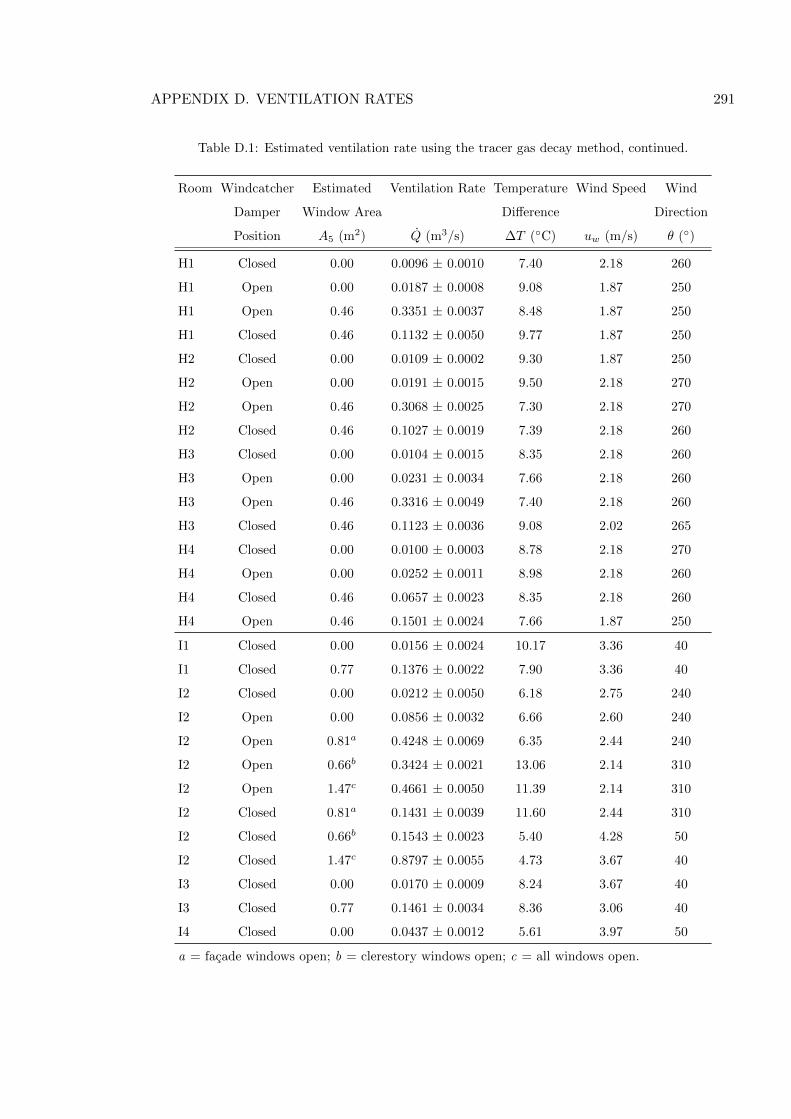
APPENDIX D. VENTILATION RATES 291
Table D.1: Estimated ventilation rate using the tracer gas decay method, continued.
Room Windcatcher Estimated Ventilation Rate Temperature Wind Speed Wind
Damper Window Area Difference Direction
Position A5 (m2) Q (m3/s) ∆T (◦C) uw (m/s) θ (◦)
H1 Closed 0.00 0.0096 ± 0.0010 7.40 2.18 260
H1 Open 0.00 0.0187 ± 0.0008 9.08 1.87 250
H1 Open 0.46 0.3351 ± 0.0037 8.48 1.87 250
H1 Closed 0.46 0.1132 ± 0.0050 9.77 1.87 250
H2 Closed 0.00 0.0109 ± 0.0002 9.30 1.87 250
H2 Open 0.00 0.0191 ± 0.0015 9.50 2.18 270
H2 Open 0.46 0.3068 ± 0.0025 7.30 2.18 270
H2 Closed 0.46 0.1027 ± 0.0019 7.39 2.18 260
H3 Closed 0.00 0.0104 ± 0.0015 8.35 2.18 260
H3 Open 0.00 0.0231 ± 0.0034 7.66 2.18 260
H3 Open 0.46 0.3316 ± 0.0049 7.40 2.18 260
H3 Closed 0.46 0.1123 ± 0.0036 9.08 2.02 265
H4 Closed 0.00 0.0100 ± 0.0003 8.78 2.18 270
H4 Open 0.00 0.0252 ± 0.0011 8.98 2.18 260
H4 Closed 0.46 0.0657 ± 0.0023 8.35 2.18 260
H4 Open 0.46 0.1501 ± 0.0024 7.66 1.87 250
I1 Closed 0.00 0.0156 ± 0.0024 10.17 3.36 40
I1 Closed 0.77 0.1376 ± 0.0022 7.90 3.36 40
I2 Closed 0.00 0.0212 ± 0.0050 6.18 2.75 240
I2 Open 0.00 0.0856 ± 0.0032 6.66 2.60 240
I2 Open 0.81a 0.4248 ± 0.0069 6.35 2.44 240
I2 Open 0.66b 0.3424 ± 0.0021 13.06 2.14 310
I2 Open 1.47c 0.4661 ± 0.0050 11.39 2.14 310
I2 Closed 0.81a 0.1431 ± 0.0039 11.60 2.44 310
I2 Closed 0.66b 0.1543 ± 0.0023 5.40 4.28 50
I2 Closed 1.47c 0.8797 ± 0.0055 4.73 3.67 40
I3 Closed 0.00 0.0170 ± 0.0009 8.24 3.67 40
I3 Closed 0.77 0.1461 ± 0.0034 8.36 3.06 40
I4 Closed 0.00 0.0437 ± 0.0012 5.61 3.97 50
a = facade windows open; b = clerestory windows open; c = all windows open.
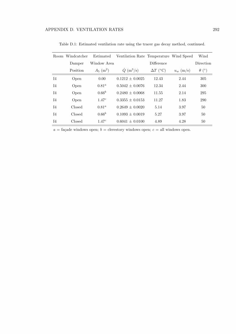
APPENDIX D. VENTILATION RATES 292
Table D.1: Estimated ventilation rate using the tracer gas decay method, continued.
Room Windcatcher Estimated Ventilation Rate Temperature Wind Speed Wind
Damper Window Area Difference Direction
Position A5 (m2) Q (m3/s) ∆T (◦C) uw (m/s) θ (◦)
I4 Open 0.00 0.1212 ± 0.0025 12.43 2.44 305
I4 Open 0.81a 0.5042 ± 0.0076 12.34 2.44 300
I4 Open 0.66b 0.2480 ± 0.0068 11.55 2.14 295
I4 Open 1.47c 0.3355 ± 0.0153 11.27 1.83 290
I4 Closed 0.81a 0.2649 ± 0.0020 5.14 3.97 50
I4 Closed 0.66b 0.1093 ± 0.0019 5.27 3.97 50
I4 Closed 1.47c 0.6041 ± 0.0100 4.89 4.28 50
a = facade windows open; b = clerestory windows open; c = all windows open.
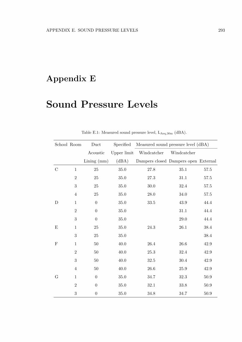
APPENDIX E. SOUND PRESSURE LEVELS 293
Appendix E
Sound Pressure Levels
Table E.1: Measured sound pressure level, LAeq,30m (dBA).
School Room Duct Specified Measured sound pressure level (dBA)
Acoustic Upper limit Windcatcher Windcatcher
Lining (mm) (dBA) Dampers closed Dampers open External
C 1 25 35.0 27.8 35.1 57.5
2 25 35.0 27.3 31.1 57.5
3 25 35.0 30.0 32.4 57.5
4 25 35.0 28.0 34.0 57.5
D 1 0 35.0 33.5 43.9 44.4
2 0 35.0 31.1 44.4
3 0 35.0 29.0 44.4
E 1 25 35.0 24.3 26.1 38.4
3 25 35.0 38.4
F 1 50 40.0 26.4 26.6 42.9
2 50 40.0 25.3 32.4 42.9
3 50 40.0 32.5 30.4 42.9
4 50 40.0 26.6 25.9 42.9
G 1 0 35.0 34.7 32.3 50.9
2 0 35.0 32.1 33.8 50.9
3 0 35.0 34.8 34.7 50.9
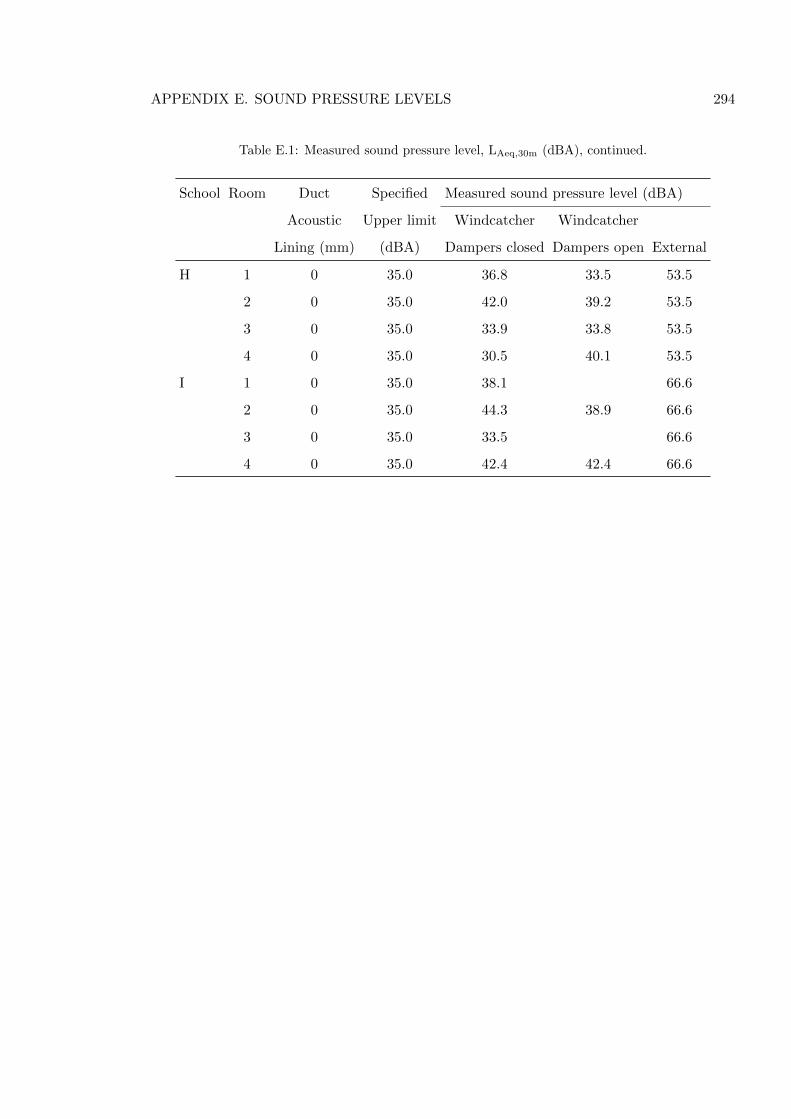
APPENDIX E. SOUND PRESSURE LEVELS 294
Table E.1: Measured sound pressure level, LAeq,30m (dBA), continued.
School Room Duct Specified Measured sound pressure level (dBA)
Acoustic Upper limit Windcatcher Windcatcher
Lining (mm) (dBA) Dampers closed Dampers open External
H 1 0 35.0 36.8 33.5 53.5
2 0 35.0 42.0 39.2 53.5
3 0 35.0 33.9 33.8 53.5
4 0 35.0 30.5 40.1 53.5
I 1 0 35.0 38.1 66.6
2 0 35.0 44.3 38.9 66.6
3 0 35.0 33.5 66.6
4 0 35.0 42.4 42.4 66.6
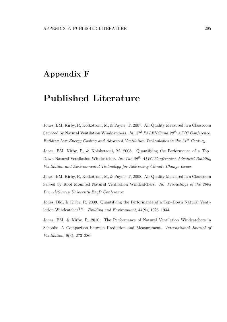
APPENDIX F. PUBLISHED LITERATURE 295
Appendix F
Published Literature
Jones, BM, Kirby, R, Kolkotroni, M, & Payne, T. 2007. Air Quality Measured in a Classroom
Serviced by Natural Ventilation Windcatchers. In: 2nd PALENC and 28th AIVC Conference:
Building Low Energy Cooling and Advanced Ventilation Technologies in the 21st Century.
Jones, BM, Kirby, R, & Kolokotroni, M. 2008. Quantifying the Performance of a Top–
Down Natural Ventilation Windcatcher. In: The 29th AIVC Conference: Advanced Building
Ventilation and Environmental Technology for Addressing Climate Change Issues.
Jones, BM, Kirby, R, Kolkotroni, M, & Payne, T. 2008. Air Quality Measured in a Classroom
Served by Roof Mounted Natural Ventilation Windcatchers. In: Proceedings of the 2008
Brunel/Surrey University EngD Conference.
Jones, BM, & Kirby, R. 2009. Quantifying the Performance of a Top–Down Natural Venti-
lation WindcatcherTM. Building and Environment, 44(9), 1925–1934.
Jones, BM, & Kirby, R. 2010. The Performance of Natural Ventilation Windcatchers in
Schools: A Comparison between Prediction and Measurement. International Journal of
Ventilation, 9(3), 273–286.