Embed Size (px)
Citation preview
Quantifying Controversy in Social Media
Kiran GarimellaAalto UniversityHelsinki, Finland
Gianmarco De Francisci MoralesAalto UniversityHelsinki, Finland
[email protected] Gionis
Aalto UniversityHelsinki, Finland
Michael MathioudakisHIIT, Aalto University
Helsinki, [email protected]
ABSTRACTWhich topics spark the most heated debates in social media?Identifying these topics is a first step towards creating sys-tems which pierce echo chambers. In this paper, we performthe first systematic methodological study of controversy de-tection using social-media network structure and content.
Unlike previous work, rather than identifying controversyin a single hand-picked topic and use domain-specific knowl-edge, we focus on comparing topics in any domain. Ourapproach to quantifying controversy is a graph-based three-stage pipeline, which involves (i) building a conversationgraph about a topic, which represents alignment of opinionamong users; (ii) partitioning the conversation graph to iden-tify potential sides of controversy; and (iii) measuring theamount of controversy from characteristics of the graph.
We perform an extensive comparison of controversy mea-sures, as well as graph building approaches and data sources.We use both controversial and non-controversial topics onTwitter, as well as other external datasets. We find that ournew random-walk-based measure outperforms existing onesin capturing the intuitive notion of controversy, and showthat content features are vastly less helpful in this task.
1. INTRODUCTIONGiven their widespread diffusion, online social media are
becoming increasingly important in the study of social phe-nomena such as peer influence, framing, bias, and controversy.Ultimately, we would like to understand how users perceivethe world through the lens of their social media feed. Forinstance, to offer users the possibility to balance their “newsdiet” [21, 22] on controversial topics by recommending con-trarian content, which supports a view that differs from whatthey are mostly exposed to [26]. However, before addressingthese advanced application scenarios, we first need to focuson the fundamental yet challenging task of distinguishingwhether a topic of discussion is controversial. Our work ismotivated by interest in observing controversies at societallevel, monitoring their evolution, and possibly understandingwhich issues become controversial and why.
The study of controversy in social media is not new; thereare many previous studies aimed at identifying and char-acterizing controversial issues, mostly around political de-bates [1, 8, 24, 25] but also for other topics [15]. And whilemost recent papers have focused on Twitter [8, 15, 24, 25],controversy in other social-media platforms, such as blogs [1]and opinion fora [2], have also been analyzed.
However, most previous papers have severe limitations.First, the majority of previous studies focus on controversyregarding political issues, and in particular, they are cen-tered around long-lasting major events, such as elections [1, 8].More crucially, most previous works can be characterizedas case studies, where controversy is identified in a sin-gle carefully-curated dataset, collected using ample domainknowledge and auxiliary domain-specific sources (e.g., anextensive list of hashtags regarding a major political event,or a list of left-leaning and right-leaning blogs).
We aim to overcome those limitations. Our goal is toidentify controversy regarding topics in any domain (e.g.,political, economical, or cultural), and in a general settings,i.e., without prior domain-specific knowledge about the topicin question. In addition, we aim at comparing different topics,in order to find the most controversial ones. These propertiesallow to deploy a system in-the-wild, and are valuable forbuilding real-world applications.
In order to enable such a versatile framework, we work withtopics that are defined in a lightweight and domain-agnosticmanner. Specifically, when focusing on Twitter, a topic canbe specified as a text query. For example, “#beefban” is aspecial keyword (a “hashtag”) that was employed by Twitterusers to signal that their posts referred to a decision of theIndian government, in March 2015, about the consumptionof beef meat in India. In this case, the query “#beefban”defines a topic of discussion, and the related activity consistsof all posts that contain the query.
We represent a topic of discussion with a conversationgraph. In such a graph, vertices represent people, and edgesrepresent conversation activity and interactions, such asposts, comments, mentions, or endorsements. Our workinghypothesis is that it is possible to analyze the conversationgraph of a topic to reveal how controversial the topic is. Inparticular, we expect the conversation graph of a controversialtopic to have a clustered structure. This hypothesis is basedon the fact that a controversial topic entails different sideswith opposing points of view, and individuals on the same sidetend to endorse and amplify each other’s arguments [1, 2, 8].
Our main contribution is to test this hypothesis. Weachieve this by studying a large number of candidate features,based on the following aspects of activity: (i) structure ofendorsements, i.e., who agrees with whom on the topic,(ii) structure of the social network, i.e., who is connectedwith whom among the participants in the conversation, (iii)content, i.e., the keywords used in the topic, (iv) sentiment,i.e., the tone (positive or negative) used to discuss the topic.
arX
iv:1
507.
0522
4v1
[cs
.SI]
18
Jul 2
015
Our study shows that, except from content-based features,all the other ones are useful in detecting controversial topics,to different extents. Particularly for Twitter, we find theendorsement features (i.e., retweets) to be the most useful.
The extracted features are then used to compute the con-troversy score of a topic. We offer a systematic definition andprovide a thorough evaluation of measures to quantify contro-versy. We employ a broad range of topics, both controversialand non-controversial ones, on which we evaluate severalmeasures, either defined in this paper or coming from theliterature [15, 25]. We find that one of our newly-proposedmeasure, based on random walks, is able to discriminatecontroversial topics with great accuracy. In addition, it alsogeneralizes well as it agrees with previously-defined measureswhen tested on datasets from existing work. We also findthat the variance of the sentiment expressed on a topic is areliable indication of controversy.
The systematic approach to quantifying controversy pre-sented in this paper can be condensed into a three-stagepipeline: (i) build a conversation graph among the users whocontribute to a topic, where edges signify that two users arein agreement, (ii) identify the potential sides of the contro-versy from the graph structure or the textual content, and(iii) quantify the amount of controversy in the graph.
The rest of this paper is organized as follows. Section 2discusses how this work fills gaps in the existing literature.Subsequently, Section 3 provides a high level description ofthe pipeline for quantifying controversy for a topic, whileSections 4, 5, and 6 detail each stage. We empirically evaluatethe proposed measures of controversy in Section 7. Section 8extends the evaluation to a few measures that do not fitthe pipeline. We conclude in Section 9 with a discussion onpossible improvements and directions for future work, as wellas lessons learned from carrying out this study.
2. RELATED WORKAnalysis of controversy in online news and social media
has attracted a lot of attention and a number of papers haveprovided very interesting case studies. In one of the first pa-pers, Adamic and Glance [1] study the linking patterns anddiscussion topics of political bloggers, focusing on blog postson the U.S. presidential election of 2004. They measure thedegree of interaction between liberal and conservative blogs,and provide evidence that conservative blogs are linking toeach other more frequently and in a denser pattern. Thesefindings are confirmed by the more recent study of Conoveret al. [8], who also study controversy in political communica-tion regarding congressional midterm elections. Using datafrom Twitter, Conover et al. identify a highly segregatedpartisan structure (present in the retweet graph, but not inthe mention graph), with limited connectivity between left-and right-leaning users. In another recent work related tocontroversy analysis in political discussion, Mejova et al. [24]identify a significant correlation between controversial issuesand the use of negative affect and biased language.
The papers mentioned so far study controversy in thepolitical domain, and provide case studies centered aroundlong-lasting major events, such as presidential elections. Inthis paper, we aim to identify and quantify controversy forany topic discussed in social media, including short-lived andad-hoc ones. The problem we study has been considered byprevious work, but the methods proposed so far are, to alarge degree, domain-specific.
The work of Conover et al. [8], discussed above, employsthe concept of modularity and graph partitioning in orderto verify (but not quantify) controversy structure of graphsextracted from discussion of political issues on Twitter. Ina similar setting, Guerra et al. [15] propose an alternativegraph-structure measure. Their measure relies on the analysisof the boundary between two (potentially) polarized com-munities, and performs better than modularity. Differentlyfrom these studies, our contribution consists in providing anextensive study of a large number of measures, including theones proposed earlier, and demonstrating clear improvementover those. We also aim at quantifying controversy in di-verse and in-the-wild settings, rather than carefully-curateddomain-specific datasets.
In a recent study, Morales et al. quantify polarity via thepropagation of opinions of influential users on Twitter [25].They validate their measure with a case study from Venezue-lan politics. Again, our methods are not only more generaland domain agnostic, but they provide more intuitive results.In a different approach, Akoglu proposes a polarization metricthat uses signed bipartite opinion graphs [2]. The approachdiffers from ours as it relies on the availability of this par-ticular type of data, which is not as readily available associal-interaction graphs.
Similarly to the papers discussed above, in our work wequantify controversy based on the graph structure of socialinteractions. In particular, it is assumed that controversialand polarized topics induce graphs with clustered structure,representing different opinions and points of view. Thisassumption relies on the concept of “echo chambers,” whichstates that opinions or beliefs stay inside communities createdby like-minded people, who reinforce and endorse the opinionsof each other. This phenomenon has been quantified in manyrecent studies [3, 4, 12, 14, 16].
A different direction for quantifying controversy followedby Choi et al. [7] and Mejova et al. [24] relies on text andsentiment analysis. Both studies focus on language foundon news articles. In our case, since we are mainly workingwith Twitter, where text is short and noisy, and since weare aiming at quantifying controversy in a domain-agnosticmanner, text analysis has its limitations. Nevertheless, weexperiment with incorporating content in our approach.
Finally, our findings on controversy have many potentialapplications on news-reading and public-debate scenarios.For instance, quantifying controversy can provide a basisfor analyzing the “news diet” of readers [21, 22], offering thechance of better information by providing recommendationsof contrarian views [26], or trying to deliberate debates [11]and connect people with opposing opinions [10, 13].
3. PIPELINEOur approach to measuring controversy is based on a
systematic way of characterizing social media activity. Weemploy a pipeline of three stages, namely graph building,graph partitioning and measuring controversy, as depictedin Figure 1. The final output of the pipeline is a value thatmeasures how controversial a topic is, with higher values
Graph Building
Graph Partitioning
Controversy Measure
Figure 1: Block diagram of the pipeline for computingcontroversy scores.

corresponding to higher degree of controversy. We provide ahigh-level description of each stage here and more details inthe sections that follow.
3.1 Building the GraphThe purpose of this stage is to build a conversation graph
that represents activity related to a single topic of discussion.In our pipeline, a topic is operationalized as a query, and thesocial media activity related to the topic consists of thoseitems (e.g., posts) that match that query. For example, inthe context of Twitter, the query might simply consist ofa keyword, such as “#ukraine”, in which case the relatedactivity consists of all tweets that contain that keyword. Eventhough we describe textual queries in standard document-retrieval form, in principle queries can take other forms, aslong as they are able to induce a graph from the social mediaactivity (e.g., RDF queries, or topic models).
Each item related to a topic is associated with one userwho generated it, and we build a graph where each user whocontributed to the topic is assigned to one vertex. In thisgraph, an edge between two vertices represents endorsment,agreement, or shared point of view between the correspondingusers. Section 4 details several ways to build such a graph.
3.2 Partitioning the GraphIn the second stage, the resulting conversation graph is fed
into a graph partitioning algorithm to extract two partitions(we defer considering multi-sided controversies to a furtherstudy). Intuitively, the two partitions correspond to twodisjoint sets of users who possibly belong to different sidesin the discussion. In other words, the output of this stageanswers the following question: “assuming that users are splitinto two sides according to their point of view on the topic,which are these two sides?” Section 5 describes this stagein further detail. If indeed there are two sides which do notagree with each other –a controversy– then the two partitionsshould be loosely connected to each other, given the semanticof edges. This property is captured by a measure computedin the third and final stage of the pipeline.
3.3 Measuring ControversyThe third and last stage takes as input the graph built
by the first stage and partitioned by the second stage, andcomputes the value of a controversy measure that character-izes how controversial the topic is. Intuitively, a controversymeasure aims to capture how separated the two partitionsare. We test several such measures, including ones based onrandom walks, betweenness centrality, and low-dimensionalembeddings. Details are provided in Section 6.
4. GRAPH BUILDINGThis section provides details about the different approaches
we follow to build graphs from raw data. We use posts onTwitter to create our datasets1. Twitter is a natural choicefor the problem at hand, as it represents one of the main forafor public debate in online social media, and is often used toreport news about current events. Following the proceduredescribed in Section 3.1, we specify a set of queries and buildone graph for each. The set of topics we choose is balancedbetween controversial and non-controversial ones, so as totest for both false positives and false negatives.
1We had access to the full Twitter firehose stream.
We use Twitter hashtags as queries. Users employ hashtagsto indicate the topic of discussion their posts pertain to.Among the large number of hashtags that appear on theTwitter stream, we consider hashtags that were trendingduring the period from Feb 27 to Jun 15, 2015. By manualinspection we find that most trending hashtags are not relatedto controversial discussions.
We first manually distinguish a set of 10 hashtags thatwe know represent controversial topics of discussion. Alltopics in this set have been widely covered by mainstreammedia, and have generated ample discussion both online andoffline. Moreover, to have a dataset that is balanced betweencontroversial and non-controversial topics, we sample anotherset of 10 hashtags that we know represent non-controversialtopics of discussion. These hashtags are related mostly tosoft news and entertainment, but also to events that, whilebeing impactful and dramatic, did not generate large con-troversies (e.g., #nepal and #germanwings). In additionto our intuition that these topics are non-controversial, wemanually checked a sample of tweets and were not able toidentify any controversy.2
For each hashtag, we retrieve all tweets that contain itand are generated during the observation window. We alsoensure that the selected hashtags are associated with a largeenough volume of activity. Table 1 presents the final set ofhashtags, along with their description and the number ofrelated tweets.3
To build a graph G for each hashtag, we assign one vertexto each user who employs the hashtag, and generate edgesaccording to one of the following four approaches.
1. Retweet graph. Typically, retweets are used as endorse-ments. Users who retweet signal endorsement of the opinionexpressed in the original tweet by propagating it further.Retweets are not constrained to occur only between userswho are connected in Twitter’s social network, but users areallowed to re-post tweets generated by any other user.
We select the edges for graph G based on the retweetactivity in the topic: an edge exists between two users u andv if there are at least two (τ = 2) retweets between them thatuse the hashtag, irrespective of direction. We remark that,in preliminary experimentation with this approach, buildingthe retweet graph with a threshold τ = 1 did not producereliable results. We presume that a single retweet on a topicis not enough of a signal to infer endorsement. Using τ = 2retweets as threshold proves to be a good trade-off betweenhigh selectivity (which hinders analysis) and noise reduction.The resulting size for each retweet graph is listed in Table 1.
2. Follow graph. In this approach, we build the followgraph induced by a given hashtag. We select the edges forgraph G based on the social connections between Twitterusers who employ the given hashtag : an edge exists betweenusers u and v if u follows v or vice-versa. We stress thatthe graph G built with this approach is topic-specific, as theedges in G are constrained to connections between users whodiscuss the topic that is specified as input to the pipeline.
The rationale for using this graph is based on an assump-tion for the presence of homophily in the social network,which is a common trait in this setting. To be more precise,
2Code and the networks we used will be available at http://github.com/gvrkiran/controversy-detection.3We use a hashtag in Russian, #marx, which we refer to as#russia march from here on, for convenience.
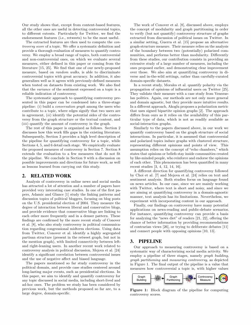
Table 1: Datasets statistics: hashtag, sizes of the follow and retweet graphs, and description of the event. The top grouprepresent controversial topics, while the bottom one represent non-controversial ones.
Hashtag # Tweets Retweet graph Follow graph Description and collection period (2015)
|V | |E| |V | |E|#beefban 84 543 1610 1978 799 6026 Government of India bans beef, Mar 2–5#nemtsov 183 477 6546 10 172 2156 46 529 Death of Boris Nemtsov, Feb 28–Mar 2#netanyahuspeech 254 623 9434 14 476 4292 297 136 Netanyahu’s speech at U.S. Congress, Mar 3–5#marx 118 629 2134 2951 1189 16 471 Protests after death of Boris Nemtsov (“march”), Mar 1–2#indiasdaughter 167 704 3659 4323 1542 9480 Controversial Indian documentary, Mar 1–5#baltimoreriots 218 157 3902 4505 1441 28 291 Riots in Baltimore after police kills a black man, Apr 28–30#indiana 116 379 2467 3143 946 24 328 Indiana pizzeria refuses to cater gay wedding, Apr 2–5#ukraine 287 438 5495 9452 3383 84 035 Ukraine conflict, Feb 27–Mar 2#gunsense 318 409 7106 11 483 1821 103 840 Gun violence in U.S., Jun 1–30#leadersdebate 1 139 344 25 983 44 174 9566 344 088 Debate during the U.K. national elections, May 3
#sxsw 343 652 9304 11 003 4558 91 356 SXSW conference, Mar 13–22#1dfamheretostay 501 960 15 292 26 819 3151 20 275 Last OneDirection concert, Mar 27–29#germanwings 907 510 29 763 39 075 2111 7329 Germanwings flight crash, Mar 24–26#mothersday 1 798 018 155 599 176 915 2225 14 160 Mother’s day, May 8#nepal 1 297 995 40 579 57 544 4242 42 833 Nepal earthquake, Apr 26–29#ultralive 364 236 9261 15 544 2113 16 070 Ultra Music Festival, Mar 18–20#FF 408 326 5401 7646 3899 63 672 Follow Friday, Jun 19#jurassicworld 724 782 26 407 32 515 4395 31 802 Jurassic World movie, Jun 12-15#wcw 156 243 10 674 11 809 3264 23 414 Women crush Wednesdays, Jun 17#nationalkissingday 165 172 4638 4816 790 5927 National kissing day, Jun 19
we expect that on a given topic people will agree more oftenthan not with people they follow, and that for a controver-sial topic of discussion this phenomenon will be reflected inwell-separated partitions of the resulting graph. Note thatusing the entire social graph would not necessarily producewell-separated partitions that correspond to single topics ofdiscussion, as those partitions would be “blurred” by theexistence of additional edges that are due to other reasons(e.g., offline social connections).
On the practical side, while the retweet information isreadily available in the stream of tweets, the social networkof Twitter is not. Collecting the follower graph thus requiresan expensive crawling phase. The resulting graph size foreach follow graph is listed in Table 1.
3. Content graph. We create the edges of graph G basedon whether users post instances of the same content. Specifi-cally, we experiment with the following three variants: createan edge between two vertices if the users (i) use the samehashtag, other than the one that defines the topic, (ii) sharea link to the same URL, or (iii) share a link with the sameURL domain (e.g., cnn.com is the domain for all pages onthe website of CNN).
4. Hybrid content & retweet graph. We create edgesfor graph G according to a state-of-the-art process thatblends content and graph information [27]. Concretely, weassociate each user with a vector of frequencies of mentionsfor different hashtags. Subsequently, we create edges betweenpairs of users whose corresponding vectors have high cosinesimilarity, and combine them with edges from the retweetgraph, built as described above. For details, we refer theinterested reader to the original publication [27].
5. GRAPH PARTITIONINGAs explained above, we use a graph-partitioning algorithm
to produce two partitions on the conversation graph. Werely on a state-of-the-art off-the-shelf algorithm, METIS [20].Figure 2 displays the two partitions returned for some ofthe topics on their corresponding retweet and follow graphs
(Figures 2(a)-(d) and Figures 2(e)-(h), respectively).4 Thepartitions are indicated in blue or red. The graph layoutis produced by Gephi’s ForceAtlas2 algorithm [17], and isbased solely on the structure of the graph, not on METIS’spartitioning.
From an initial visual inspection of the partitions identifiedon retweet and follow graphs, we find that the partitionsmatch well with our intuition of which topics are controver-sial (the partitions returned by METIS are well separated forcontroversial topics). To make sure that this initial assess-ment of the partitions is not an artifact of the visualizationalgorithm we use, we try other layouts offered by Gephi.In all cases we observe similar patterns. We also manuallysample and check tweets from the partitions, to verify thepresence of controversy. While this anecdotal evidence ishard to report, indeed the partitions seem to capture thespirit of the controversy.5
On the contrary, the partitions identified on content graphsfail to match our intuition. All three variants of the content-based approach lead to sparse graphs and highly overlappingpartitions, even in cases of highly controversial issues. Thesame pattern applies for the hybrid approach, as shown inFigure 3. We also try a variant of the hybrid graph approachwith vectors that represent the frequency of different URLdomains mentioned by a user, with no better results. Wethus do not consider these approaches to graph building anyfurther in the remainder of this paper.
Finally, we also try different types of graph partitioningalgorithms from different classes. Apart from METIS (cutbased), we test spectral clustering, label propagation, andaffiliation-graph-based models. The difference among allthese methods is not significant, however from visual inspec-tion METIS generates the cleanest partitions.
4Other topics show similar trends, omitted for lack of space.5For instance, of these two tweets for #netanyahuspeech fromtwo users on either side, one is clearly supporting the speechhttps://t.co/OVeWB4XqIg, while the other highlights thenegative reactions https://t.co/v9RdPudrrC.

(a) (b) (c) (d)
(e) (f) (g) (h)
Figure 2: Sample conversation graphs with retweet (top) and follow (bottom) features (visualized using the force directedlayout algorithm in Gephi). The left side is controversial, (a,e) #beefban, (b,f) #russia march, while the right side isnon-controversial, (c,g) #sxsw, (d,h) #germanwings.
(a) (b)
Figure 3: Partitions obtained for (a) #beefban, (b) #rus-sia march using the hybrid graph building approach. Thepartitions are much more noisy than those in Figures 2(a,b).
6. CONTROVERSY MEASURESThis section describes several controversy measures used in
this work. For completeness, we describe both those measuresproposed by us (§6.1, 6.2, 6.3) as well as the ones from theliterature that we use as baselines (§6.4, 6.5).
6.1 Random walkThis measure uses the notion of random walks on graphs.
It is based on the rationale that, in a controversial discussion,there are authoritative users on both sides, as evidencedby a large degree in the graph. The measure captures theintuition of how likely a random user on either side is to beexposed to authoritative content from the opposing side.
Let G(V,E) be the graph built by the first stage and its
two partitions X and Y , (X ∪ Y = V , X ∩ Y = ∅) identifiedby the second stage of the pipeline. We first distinguish thek highest-degree vertices from each partition. High-degreeis a proxy for authoritativeness, as it means that a user hasreceived a large number of endorsements on the specific topic.Subsequently, we select one partition at random (each withprobability 0.5) and consider a random walk that starts froma random vertex in that partition. The walk terminates whenit visits any high-degree vertex (from either side).
We define the Random Walk Controversy (RWC ) measureas follows. “consider two random walks, one ending in parti-tion X and one ending in partition Y , RWC is the differenceof the probabilities of two events: (i) both random walksstarted from the partition they ended in and (ii) both randomwalks started in a partition other than the one they ended in.”The measure is quantified as
RWC = PXXPY Y − PY XPXY , (1)
where PAB , A,B ∈ {X,Y } is the conditional probability
PAB = P (start in partition A | end in partition B).
Note that the aforementioned probabilities have the followingdesirable properties: (i) they are not skewed by the size ofeach partition, as the random walk starts with equal proba-bility from each partition, and (ii) they are not skewed by thetotal degree of vertices in each partition, as the probabilitiesare conditional on ending in either partition (i.e., the ratio ofrandom walks ending in partition X/Y is irrelevant). RWCis close to one when the probability of crossing sides is low,and close to zero when the probability of crossing sides iscomparable to that of staying on the same side.
6.2 BetweennessLet us consider the set of edges C ⊆ E in the cut defined
by the two partitions X,Y . This measure uses the notion ofedge betweenness and how the betweenness of the cut differsfrom that of the other edges. Recall that the betweennesscentrality bc(e) of an edge e is defined as
bc(e) =∑
s6=t∈V
σs,t(e)
σs,t, (2)
where σs,t is the total number of shortest paths betweenvertices s, t in the graph and σs,t(e) is the number of thoseshortest paths that include edge e.
The intuition here is that, if the two partitions are well-separated, then the cut will consist of edges that bridgestructural holes [6]. In this case, the shortest paths thatconnect vertices of the two partitions will pass through theedges in the cut, leading to high betweenness values for edgesin C. On the other hand, if the two partitions are not wellseparated, then the cut will consist of strong ties. In this case,the paths that connect vertices across the two partitions willpass through one of the many edges in the cut, leading tobetweenness values for C similar to the rest of the graph.
Given the distributions of edge betweenness on the cut andthe rest of the graph, we compute the KL divergence dKL
of the two distributions by using kernel density estimationto compute the PDF and sampling 10 000 points from eachof these distributions (with replacement). We define theBetweenness Centrality Controversy (BCC ) measure as
BCC = 1− e−dKL , (3)
which assumes values close to zero when the divergence issmall, and close to one when the divergence is large.
6.3 EmbeddingThis measure is based on a low-dimensional embedding
of graph G produced by Gephi’s ForceAtlas2 algorithm [17](the same algorithm that was used to produce the plots inFigures 2 and 3). We opt for this algorithm as it produceswell-separated plots for controversial topics.
Let us consider the two-dimensional embedding φ(v) ofvertices v ∈ V produced by ForceAtlas2. Given the partitionX, Y produced by the second stage of the pipeline, wecalculate the following quantities:
• dX and dY , the average embedded distance among pairsof vertices in the same partition X and Y , respectively,
• dXY , the average embedded distance among pairs ofvertices across the two partitions X and Y .
Inpsired by the Davies-Bouldin (DB) index [9], we define theEmbedding Controversy measure EC as
EC = 1− dX + dY
2dXY
. (4)
EC is close to one for controversial topics, correspondingto better-separated graphs and thus to higher degree ofcontroversy, and close to zero for non-controversial topics.
6.4 Boundary ConnectivityThis controversy measure was proposed by Guerra et al.
[15] and is based on the notion of boundary and internalvertices. Let u ∈ X be a vertex in partition X; u belongsto the boundary of X iff it is connected to at least one
vertex of the other partition Y , and it is connected to atleast one vertex in partition X that is not connected toany vertex of partition Y . Following this definition, letBX , BY be the set of boundary vertices for each partition,and B = BX ∪ BY the set of all boundary vertices. Bycontrast, vertices IX = X −BX are said to be the internalvertices of partition X (similarly for IY ). Let I = IX ∪ IY beall internal vertices in either partition. The rationale for thismeasure is that, if the two partitions represent two sides ofa controversy, then boundary vertices will be more stronglyconnected to internal vertices than other boundary verticesof either partition. This is captured in the formula:
GMCK =1
|B|∑u∈B
di(u)
db(u) + di(u)− 0.5 (5)
where di(u) is the number of edges between vertex u andinternal vertices I, while db(u) is the number of edges betweenvertex u and boundary vertices B. Higher values of themeasure correspond to higher degrees of controversy.
6.5 Dipole MomentThis controversy measure was presented by Morales et al.
[25] and it is based on the notion of dipole moment that hasits origin in physics. Let R(u) ∈ [−1, 1] be a polarizationvalue assigned to vertex u ∈ V . Intuitively, extreme valuesof R (close to −1 or 1) correspond to users who belong mostclearly to either side of the controversy. To set the values R(u)we follow the process described in the original paper [25]:we set R = ±1 for the top-5% highest-degree vertices ineach partition X and Y , and set the values for the rest ofthe vertices by label-propagation. Let n+ and n− be thenumber of vertices V with positive and negative polarizationvalues, respectively, and ∆A the absolute difference of their
normalized size: ∆A =∣∣∣n+−n−
|V |
∣∣∣ . Moreover, let gc+ (gc−)
be the average polarization value among vertices n+ (n−)
and set d as half their absolute difference, d =|gc+−gc−|
2.
The dipole moment controversy measure is defined as
MBLB = (1−∆A)d. (6)
The rationale for this measure is that if the two partitions Xand Y are well separated, then label propagation will assigndifferent extreme (±1) R-values to the two partitions, leadingto higher values of the MBLB measure. Note also that largerdifferences in the size of the two partitions (reflected in thevalue of ∆A) lead to decreased values for the measure, whichtakes values between zero and one.
7. EXPERIMENTSIn this section we report the results of the various configu-
rations of the pipeline proposed in this paper. As previouslystated, we omit results for the content and hybrid graphbuilding approaches presented in Section 4 as they do notperform well. We instead focus on the retweet and followgraphs, and test all the measures presented in Section 6 onthe Twitter topics described in Table 1. In addition, wetest all the measures on a set of external datasets used inprevious studies [1, 8, 15] to validate the measures against aknown ground truth. Finally, we use an evolving dataset fromTwitter collected around the death of Venezuelan presidentHugo Chavez [25] to show the evolution of the controversymeasures in response to high-impact events.
0.0
0.2
0.4
0.6
0.8
1.0
BCC EC GMCK MBLB RWC
Con
trov
ersy
sco
re
ControversialNon−controversial
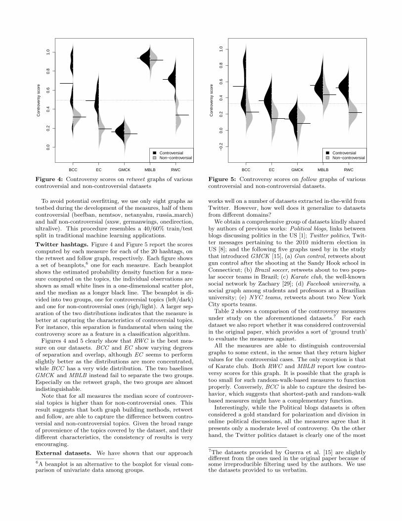
Figure 4: Controversy scores on retweet graphs of variouscontroversial and non-controversial datasets
To avoid potential overfitting, we use only eight graphs astestbed during the development of the measures, half of themcontroversial (beefban, nemtsov, netanyahu, russia march)and half non-controversial (sxsw, germanwings, onedirection,ultralive). This procedure resembles a 40/60% train/testsplit in traditional machine learning applications.
Twitter hashtags. Figure 4 and Figure 5 report the scorescomputed by each measure for each of the 20 hashtags, onthe retweet and follow graph, respectively. Each figure showsa set of beanplots,6 one for each measure. Each beanplotshows the estimated probability density function for a mea-sure computed on the topics, the individual observations areshown as small white lines in a one-dimensional scatter plot,and the median as a longer black line. The beanplot is di-vided into two groups, one for controversial topics (left/dark)and one for non-controversial ones (righ/light). A larger sep-aration of the two distributions indicates that the measure isbetter at capturing the characteristics of controversial topics.For instance, this separation is fundamental when using thecontroversy score as a feature in a classification algorithm.
Figures 4 and 5 clearly show that RWC is the best mea-sure on our datasets. BCC and EC show varying degreesof separation and overlap, although EC seems to performslightly better as the distributions are more concentrated,while BCC has a very wide distribution. The two baselinesGMCK and MBLB instead fail to separate the two groups.Especially on the retweet graph, the two groups are almostindistinguishable.
Note that for all measures the median score of controver-sial topics is higher than for non-controversial ones. Thisresult suggests that both graph building methods, retweetand follow, are able to capture the difference between contro-versial and non-controversial topics. Given the broad rangeof provenience of the topics covered by the dataset, and theirdifferent characteristics, the consistency of results is veryencouraging.
External datasets. We have shown that our approach
6A beanplot is an alternative to the boxplot for visual com-parison of univariate data among groups.
−0.
20.
00.
20.
40.
60.
81.
0
BCC EC GMCK MBLB RWC
Con
trov
ersy
sco
re
ControversialNon−controversial
Figure 5: Controversy scores on follow graphs of variouscontroversial and non-controversial datasets.
works well on a number of datasets extracted in-the-wild fromTwitter. However, how well does it generalize to datasetsfrom different domains?
We obtain a comprehensive group of datasets kindly sharedby authors of previous works: Political blogs, links betweenblogs discussing politics in the US [1]; Twitter politics, Twit-ter messages pertaining to the 2010 midterm election inUS [8]; and the following five graphs used by in the studythat introduced GMCK [15], (a) Gun control, retweets aboutgun control after the shooting at the Sandy Hook school inConnecticut; (b) Brazil soccer, retweets about to two popu-lar soccer teams in Brazil; (c) Karate club, the well-knownsocial network by Zachary [29]; (d) Facebook university, asocial graph among students and professors at a Brazilianuniversity; (e) NYC teams, retweets about two New YorkCity sports teams.
Table 2 shows a comparison of the controversy measuresunder study on the aforementioned datasets.7 For eachdataset we also report whether it was considered controversialin the original paper, which provides a sort of ‘ground truth’to evaluate the measures against.
All the measures are able to distinguish controversialgraphs to some extent, in the sense that they return highervalues for the controversial cases. The only exception is thatof Karate club. Both RWC and MBLB report low contro-versy scores for this graph. It is possible that the graph istoo small for such random-walk-based measures to functionproperly. Conversely, BCC is able to capture the desired be-havior, which suggests that shortest-path and random-walkbased measures might have a complementary function.
Interestingly, while the Political blogs datasets is oftenconsidered a gold standard for polarization and division inonline political discussions, all the measures agree that itpresents only a moderate level of controversy. On the otherhand, the Twitter politics dataset is clearly one of the most
7The datasets provided by Guerra et al. [15] are slightlydifferent from the ones used in the original paper because ofsome irreproducible filtering used by the authors. We usethe datasets provided to us verbatim.

Table 2: Results on external datasets. The ‘C?’ column indicates whether the previous study considered the datasetcontroversial (ground truth).
Dataset |V | |E| C? RWC BCC EC GMCK MBLB
Political blogs 1222 16 714 3 0.42 0.53 0.49 0.18 0.45Twitter politics 18 470 48 053 3 0.77 0.79 0.62 0.28 0.34Gun control 33 254 349 782 3 0.70 0.68 0.55 0.24 0.81Brazil soccer 20 594 82 421 3 0.67 0.48 0.68 0.17 0.75Karate club 34 78 3 0.11 0.64 0.51 0.17 0.11Facebook university 281 4389 7 0.35 0.26 0.38 0.01 0.27NYC teams 95 924 176 249 7 0.34 0.24 0.17 0.01 0.19
DaysD-2
9D-2
7D-2
5D-2
3D-2
1D-1
9D-1
7D-1
5D-1
3D-1
1D-9
D-7
D-5
D-3
D-1
D+1
D+3
D+5
D+7
D+9
D+1
1
D+1
3
D+1
5
D+1
6
D+1
8
D+2
0
D+2
2
D+2
4
Contr
overs
y s
core
0
0.1
0.2
0.3
0.4
0.5
0.6
0.7
0.8
0.9
1MBLBRWCECGMCKBCC
Figure 6: Controversy scores on 56 retweet graphs from Morales et al. Day ‘D’ (indicated by the blue vertical line) indicatesthe announcement of the death of president Hugo Chavez.
controversial one across all measures. This difference mightsuggest that the measures are more geared towards capturingthe dynamics of controversy as it unfolds on social media,which might differ from more traditional blogs. For instance,one such difference is the cost of an endorsement: placing alink on a blog post arguably consumes more mental resourcesthan clicking the retweet button.
For the Gun control dataset, Guerra et al. needs to manu-ally distinguish three different partitions in the graph, gunrights advocates, gun control supporters, and moderates.Our pipeline is able to find the two communities with oppos-ing views (grouping gun control supporters and moderates)without any external help. All measures agree with theconclusions in the original paper that this topic is highlycontroversial.
Evolving controversy. We have shown that our approachalso generalizes well to datasets from different domains. Butin a real deployment the measures need to be computedcontinuously, as new data arrives. How well does our methodwork in such a setting? And how do the controversy measuresevolve in response to high-impact events?
To answer these questions we use a datasets from the studythat introduced MBLB [25]. The dataset comprises Twittermessages pertaining to political events in Venezuela aroundthe time of death of Hugo Chavez (Feb-May 2013). Theauthors built a retweet graph for each of the 56 days (onegraph per day) around the day of the death.
Figure 6 shows how the intensity of controversy evolvesaccording to the measures under study (which occurs on day
‘D’). The measure proposed in the original paper, MBLB ,which we use as ‘ground truth’, shows a clear decrease ofcontroversy on the day of the death, followed by a progressiveincrease in the controversy of the conversation. The originalinterpretation states that on the day of the death a largeamount of people, also from other countries, retweeted newsof the event, creating a single global community that gottogether at the shock of the news. After the death, the rulingand opposition party entered in a fiery discussion over thenext elections, which increased the controversy.
All the measures proposed in this work show the sametrend as MBLB . Both RWC and EC follow very closely theoriginal measure (Pearson correlation coefficients r of 0.944and 0.949, respectively), while BCC shows a more jaggedbehavior in the first half of the plot (r = 0.743), due tothe discrete nature of shortest paths. All measures howeverpresent a dip on day ‘D’, an increase in controversy in thesecond half, and another dip on day ‘D+20’. Conversely,GMCK reports an almost constant moderate value of con-troversy during the whole period (r = 0.542), with barelynoticeable peaks and dips. We conclude that our measuresgeneralize well also to the case of evolving graphs, and behaveas expected in response to high-impact events.
8. CONTENTIn this section we explore alternative approaches to mea-
suring controversy that use only the content of the discussionrather than the structure of user interactions. As such, thesemethods do not fit in the pipeline described in Section 3.

The question we address is “does content help in measuringthe controversy of a topic?”. In particular, we test with twotypes of features extracted from the content. The first, is atypical IR-inspired bag-of-words representation. The secondinstead is based on NLP tools for sentiment analysis.
8.1 Content as bag of wordsWe take in input the raw content of the social media
posts, in our case the Tweets containing a specific hashtag.We represent each tweet as a vector in a high-dimensionalspace composed of the words used in the whole topic, afterstandard preprocessing used in IR (lowercasing, stopwordremoval, stemming). Following the lines of our main pipeline,we group these vectors in two clusters by using CLUTO [19]with cosine distance.
The underlying assumption is that the two sides, whilesharing the use of the hashtag for the topic, use differentvocabularies in reference to the issue at hand. For example,for #beefban a side may be calling for “freedom” while theopposing one for “respect”. We use KL divergence as ameasure of distance between the vocabularies of the twoclusters, and the I2 measure [23] of clustering heterogeneity.
We use an unpaired Wilcoxon rank-sum test at the p = 0.05significance level, but we are unable to reject the null hypoth-esis that there is no difference in these measures betweenthe controversial and non-controversial topics. Therefore,there is not enough signal in the content representation todiscern between controversial and non-controversial topicswith enough confidence. This result suggests that the bag-of-words representation of content is not a good basis forour task. It also agrees with our earlier attempts to use con-tent to build the graph used in the pipeline (see Section 4) –which suggests that using content for the task of quantifyingcontroversy might not be straightforward.
8.2 Sentiment AnalysisNext, we resort to NLP techniques for sentiment analy-
sis to analyze the content of the discussion. We use Sen-tiStrength [28] trained on tweets to give a sentiment scorein [−4, 4] to each tweet for a given topic. In this case wedo not try to cluster tweets by their sentiment. Rather, weanalyze the difference in distribution of sentiment betweencontroversial and non-controversial topics.
While it is not possible to say that controversial topicsare more positive or negative than non-controversial ones(results omitted due to space constraints), we can detect adifference in their variance. Indeed, controversial topics havea higher variance than non-controversial ones, as shown inFigure 7. Controversial ones have a variance of at least 2,while non-controversial ones have a variance of at most 1.5.
In practice, the “tones” with which controversial topics aredebated is stronger, and sentiment analysis is able to detectthis aspect. While this signal is clear, it is not straightforwardto incorporate it into the measures based on graph structure.Moreover, this feature relies on technologies that do not workreliably for languages other than English and hence cannotbe applied for topics such as #russia march.
9. DISCUSSIONThe task we tackle in this work is certainly not an easy
one, and this study has some limitations, which we discussin this section. We also report a set of negative results thatwe produced while coming up with the measures presented.
0.0 0.5 1.0 1.5 2.0 2.5 3.0
Sen
timen
t Var
ianc
e ControversialNon−controversial
Figure 7: Sentiment variance controversy score for contro-versial and non-controversial topics.
We believe these results will be very useful in steering thisresearch topic in a fruitful direction.
9.1 LimitationsTwitter only. We present our findings mostly on datasetscoming from Twitter. While this is certainly a limitation,Twitter is one of the main venues for online public discussion,and one of the few for which data is available. Hence, Twitteris a natural choice. In addition, our measures generalize wellto datasets from other social media and the Web.
Choice of data. We manually pick the controversial topicsin our dataset, which might introduce bias. In our choice werepresent a broad set of typical controversial issues comingfrom religious, societal, racial, and political domains. Unfor-tunately, ground truths for controversial topics are hard tofind, especially for ephemeral issues. However, the topics areunanimously judged controversial by the authors. Moreover,the hashtags represent the intuitive notion of controversy thatwe strive to capture, so human judgement is an importantingredient we want to use.
Overfitting. While this work presents the largest systematicstudy on controversy in social media so far, we use only 20topics for our main experiment. Given the small number ofexamples, the risk of overfitting our measures to the datasetis real. We reduce this risk by using only 40% of the topicsduring the development of the measures. Additionally, ourmeasures agree with previous independent results on externaldatasets, which further decreases the likelihood of overfitting.
Reliance on graph partitioning. Our pipeline relies ona graph partitioning stage, whose quality is fundamental forthe proper functioning of the controversy measures. Giventhat graph partitioning is a hard but well studied problem,we rely on off-the-shelf techniques for this step. A measurethat bypasses this step entirely is highly desirable, and wereport a few unsuccessful attempts in the next subsection.
Multisided controversies. Not all controversies involveonly two sides with opposing views. Some times discussionsare multifaceted, or there are three or more competing viewson the field. The principles behind our measures neatlygeneralize to multisided controversies. However, in this casethe graph partitioning component needs to automaticallyfind the optimal number of partitions. We defer experimentalstudy of such cases to an extended version of this paper.
9.2 Negative ResultsWe briefly review a list of methods that failed to produce
reliable results and were discarded early in the process ofrefining our controversy measures.
Mentions graph. Conover et al. [8] rely on the mentiongraph in Twitter to detect controversies. However, in ourdataset the mention graphs are extremely sparse given that

we focus on short-lived events. Merging the mentions into theretweet graph does not provide any noticeable improvement.
Previous studies have also shown that people retweet simi-lar ideologies but mention across ideologies [5]. We exploitthis intuition by using correlation clustering for graph parti-tioning, with negative edges for mentions. Alas, the resultsare qualitatively worse than those obtained by METIS.
Cuts. Simple measures such as size of the cut of the parti-tions do not generalize across different graphs. Conductance(in all its variants) also yields poor results. Prior work iden-tifies controversies by comparing the structure of the graphwith randomly permuted ones [8]. Unfortunately, we obtainequally poor results by using the difference in conductancewith cuts obtained by METIS and by random partitions.
Community structure. Good community structure inthe conversation graph is often understood as a sign thatthe graph is polarized or controversial. However, this isnot always the case. We find that both assortativity andmodularity (which have been previously used to identifycontroversy) do not correlate with the controversy scores,and are not good predictors for how controversial a topic is.The work by Guerra et al. [15] presents clear arguments andexamples of why modularity should be avoided.
Partitioning. As already mentioned, bypassing the graphpartitioning to compute the measure is desirable. We explorethe use of the all pairs expected hitting time computed usingsim rank [18]. We compute the of SPID (ratio of variance tomean) of this distribution, however results are mixed.
9.3 ConclusionsIn this paper, we performed the first large-scale systematic
study for quantifying controversy in social media. We haveshown that previously-used measures are not reliable anddemonstrated that controversy can be identified both in theretweet and topic-induced follow graph. We have also shownthat simple content-based representations do not work ingeneral, while sentiment analysis offers promising results.
Among the measures we studied, the random-walk-basedRWC most neatly separates controversial topics from non-controversial ones. Besides, our measures gracefully general-ize to datasets from other domains and previous studies.
This work opens several avenues for future research. First,it is worth exploring alternative approaches and testing addi-tional features, such as, following a generative-model-basedapproach, or exploiting the temporal evolution of the dis-cussion of a topic. From the application point of view, thecontroversy score can be used to generate recommendationsthat foster a healthier “news diet” on social media.
10. REFERENCES[1] L. A. Adamic and N. Glance. The political blogosphere and
the 2004 us election: divided they blog. In LinkKDD, pages36–43, 2005.
[2] L. Akoglu. Quantifying political polarity based on bipartiteopinion networks. In ICWSM, 2014.
[3] J. An, D. Quercia, and J. Crowcroft. Partisan sharing:facebook evidence and societal consequences. In COSN,pages 13–24, 2014.
[4] E. Bakshy, S. Messing, and L. Adamic. Exposure toideologically diverse news and opinion on facebook. Science,page aaa1160, 2015.
[5] A. Bessi, G. Caldarelli, M. Del Vicario, A. Scala, andW. Quattrociocchi. Social determinants of content selection
in the age of (mis) information. In Social Informatics, pages259–268. 2014.
[6] R. S. Burt. Structural holes: The social structure ofcompetition. Harvard university press, 2009.
[7] Y. Choi, Y. Jung, and S.-H. Myaeng. Identifyingcontroversial issues and their sub-topics in news articles. InIntelligence and Security Informatics, pages 140–153.Springer, 2010.
[8] M. Conover, J. Ratkiewicz, M. Francisco, B. Goncalves,F. Menczer, and A. Flammini. Political Polarization onTwitter. In ICWSM, 2011.
[9] D. L. Davies and D. W. Bouldin. A cluster separationmeasure. IEEE TPAMI, 1(2):224–227, 1979.
[10] A. Doris-Down, H. Versee, and E. Gilbert. Political blend:an application designed to bring people together based onpolitical differences. In C&T, pages 120–130, 2013.
[11] K. M. Esterling, A. Fung, and T. Lee. How MuchDisagreement is Good for Democratic Deliberation? TheCaliforniaSpeaks Health Care Reform Experiment. SSRN,2010.
[12] S. R. Flaxman, S. Goel, and J. M. Rao. Filter bubbles, echochambers, and online news consumption, 2015.
[13] E. Graells-Garrido, M. Lalmas, and D. Quercia. Dataportraits: Connecting people of opposing views. arXivpreprint arXiv:1311.4658, 2013.
[14] C. Grevet, L. G. Terveen, and E. Gilbert. Managingpolitical differences in social media. In CSCW, pages1400–1408, 2014.
[15] P. H. C. Guerra, W. Meira Jr, C. Cardie, and R. Kleinberg.A measure of polarization on social media networks based oncommunity boundaries. In ICWSM, 2013.
[16] A. Hermida, F. Fletcher, D. Korrell, and D. Logan. Yourfriend as editor: the shift to the personalized social newsstream. In Future of Journalism Conference, pages 8–9,2011.
[17] M. Jacomy, T. Venturini, S. Heymann, and M. Bastian.ForceAtlas2, a continuous graph layout algorithm for handynetwork visualization designed for the Gephi software, 2014.
[18] G. Jeh and J. Widom. SimRank: A measure ofstructural-context similarity. In KDD, pages 538–543, 2002.
[19] G. Karypis. CLUTO - A clustering toolkit, 2002.[20] G. Karypis and V. Kumar. Metis - unstructured graph
partitioning and sparse matrix ordering system, 1995.[21] J. Kulshrestha, M. B. Zafar, L. E. Noboa, K. P. Gummadi,
and S. Ghosh. Characterizing information diets of socialmedia users. In ICWSM, 2015.
[22] M. LaCour. A balanced news diet, not selective exposure:Evidence from a direct measure of media exposure. SSRN,2012.
[23] U. Maulik and S. Bandyopadhyay. Performance evaluationof some clustering algorithms and validity indices. IEEETPAMI, 24(12):1650–1654, 2002.
[24] Y. Mejova, A. X. Zhang, N. Diakopoulos, and C. Castillo.Controversy and sentiment in online news. Symposium onComputation + Journalism, 2014.
[25] A. Morales, J. Borondo, J. Losada, and R. Benito.Measuring political polarization: Twitter shows the twosides of Venezuela. Chaos, 25(3), 2015.
[26] S. A. Munson, S. Y. Lee, and P. Resnick. Encouragingreading of diverse political viewpoints with a browser widget.In ICWSM, 2013.
[27] Y. Ruan, D. Fuhry, and S. Parthasarathy. Efficientcommunity detection in large networks using content andlinks. In WWW, pages 1089–1098, 2013.
[28] M. Thelwall. Heart and soul: Sentiment strength detectionin the social web with sentistrength. Proceedings of theCyberEmotions, pages 1–14, 2013.
[29] W. Zachary. An information flow model for conflict andfission in small groups. J. of Anthropological Research, 33:452–473, 1977.