QUANTIFICATION AND EVALUATION OF RAIL FLAW …

QUANTIFICATION AND EVALUATION OF RAIL FLAW INSPECTION PRACTICES AND TECHNOLOGIES

1,*Anish Poudel, 1Brian Lindeman, and 2Robert Wilson

1Transportation Technology Center, Inc., Pueblo, CO 81001 U.S.A. *Email: [email protected]; O: (719) 584-0553 ext. 1553

2USDOT FRA, Office of Research, Development, and Technology, Washington, DC 20590

NUMBER OF WORDS: 4,896 ASBTRACT The rail integrity research efforts by the Federal Railroad Administration (FRA) and the Association of American Railroads (AAR) are directed toward increasing safety and reliability of rail transportation. Non-destructive evaluation (NDE) technologies are critical to these efforts as they find defects in rails before they lead to failure. Current FRA-funded project efforts include expanding the Rail Flaw Library of Associated Defects (RF-LOAD) and using ultrasonic simulation/modeling for detecting internal flaws in rails. These will help improve reliability of ultrasonic NDE inspection/procedures for rail flaw detection and characterization, and support future research in detecting rail flaws as well as the methods for quantifying them. This paper provides the background on the Transportation Technology Center, Inc. (TTCI) rail inspection projects funded by the FRA and discusses the current efforts on rail flaw inspection research. This paper also provides the information on the rail flaw library samples containing artificial reflectors mimicking transverse defects (TD) as well as naturally occurring service induced flaws. Rail flaw samples include rail profiles with different amounts of wear and surface conditions. These rail flaw samples were characterized with a high level of accuracy and using established ultrasonic NDE procedures. Flaw characterization studies conducted have demonstrated that hand-held phased array UT (PAUT) is more accurate than conventional hand-held UT measurements. These rail flaw samples and 3-D Solidworks models of the rails with internal flaws are available to other rail researchers and industry service providers in the United States to support rail inspection research. Ultrasonic beam modeling simulation for different rail profiles were carried out using different angled ultrasonic transducers. Comparison of 0-degree, 37.5-degree, and 70-degree beam simulations was carried out under different rail head conditions. Characteristics of the echo responses changed significantly with respect to the change in the rail head profile.

INTRODUCTION Ultrasonic testing (UT) non-destructive evaluation (NDE) methods for rail flaw detection are the primary method employed by railroads in the U.S. to monitor, detect, and characterize rail defects on a regular basis to ensure safety, structural integrity, and reliability of the railroads (1,2). This technology usually is implemented on a hi-rail vehicle platform (commonly referred to as rail detector cars) and also is used for the start-stop-hand verify operations. Rail detector cars use fixed angle piezoelectric transducers housed in a liquid filled membrane (tire) called roller search units (RSUs) to generate/emit ultrasonic waves in the rail. Transducers are fixed and are arranged in various configurations to offer different inspection capabilities to find different types of internal defects in rails. Both normal and angle-beam ultrasonic techniques are used, as are both pulse-echo and pitch-catch techniques. Usually, two RSUs are implemented per rail in such a way that some of the transducers (37.5-degree and 70-degree) are oriented in a forward and backward position in the RSU. This configuration allows detection of defects in various orientations in the rail and minimizes the possibility of strong reflections being produced internally in the wheel, which may interfere with echoes produced in the rail. Similarly, 70-degree probes are positioned off-center from the running surface (gage and field side) to provide coverage to the gage and the field side of the rail. In addition, the side looker transducers are mounted in such a way that they are sensitive to vertical and shear type defects. Each RSU houses about six transducers with a total of as many as 12 transducers per rail. Table 1 shows different types of transducers commonly used and Figure 1 shows the schematic of

mailto:[email protected]

the ultrasonic transducers configuration in RSUs. The angles shown are not the direction of the transducer in the wheel but are the refracted angles in the rail steel. Similarly, for the start-stop-hand verify operations, a hand-held flaw detector is used to verify and size the indications detected from the detector car so proper remedial action can be taken. For this, different transducer types are used depending on the flaw types encountered. North American railroads have started adopting a continuous non-stop rail flaw inspection approach. In this approach, a detector car operates as a data-collection vehicle, continuously moving forward without stopping to verify indications and detected flaws are then later verified by hand-UT testing (1).

Table 1. Transducer orientation and targeted flaw types.

Transducers Types Target Flaw Types

0-degree Flaws oriented horizontally [Shells, Horizontal Split Head (HSH), Split Web]

37.5-degree or 45-degree Bolt Hole Cracks, Web Defects

70-degree Transverse Defects (TDs) Vertical Split Heads (VSH)

Weld Defects (porosity, inclusions, etc.)

Figure 1. Ultrasonic transducer configurations in RSUs. Ray trace is displayed as a single line but

in reality, an array of the ultrasonic beam is transmitted and received. Although conventional ultrasonic inspection systems have proven effective at finding most of the critical rail flaws, inherent limitations leave some flaws being undetected (about 10 percent) during the periodic inspection, which are only discovered after the rail breaks (3). One of the major limitations of existing conventional ultrasonic systems lies with the fixed angled inspection approach and not automatically compensating the ultrasonic beam path in worn rail head profiles. Overall, ultrasonic detection greatly depends on the magnitude of the received/recorded ultrasonic reflection from the flaw. The physical shape, size, location, and orientation of flaws, poor ultrasonic coupling, off-calibration of the instruments, and misalignment of RSUs with respect to the railhead will result in a low-amplitude reflection signal. Most importantly, the detection of internal defects in the presence of surface flaws/sub-surface shelling can be a great challenge. Rail flaw inspection reliability can be significantly influenced by several factors, including the environment in which rails are inspected and human error. North American railroads operate under various temperature and humidity. The temperature ranges from -40°F to +120°F (40°C to +49°C) and atmosphere ranges from extremely dry to rain, snow, and fog. Proper education and training of NDE personnel for rail flaw detection and characterization are a must and extremely important. To address the needs of enhanced/improved rail flaw inspection, research at TTCI currently is focused on expanding RF-LOAD and optimizing ultrasonic parameters via conducting ultrasonic beam modeling and

inspection simulation for commonly missed internal rail defects. This paper will provide a brief overview of these efforts. RAIL FLAW LIBRARY OF ASSOCIATED DEFECTS (RF-LOAD) The RF-LOAD consists of master gauge samples containing a variety of artificial reflectors mimicking TD type defects as well as naturally occurring rail flaw defects. Artificial reflectors manufactured represent flat bottom holes (FBHs) of differing cross-sectional area drilled in the smaller segments of rail samples (15-24 inches). FBHs were drilled at different orientation and location relative to the railhead center point drilled. Finally, FBHs were press-fitted with dowel pins/rods (of similar material properties) to mask the holes. Master gauge rail samples include 136-RE rails with the normal head profiles (light head wear), surface damaged profiles, and curve worn (gage face wear) profiles obtained from the high tonnage loop (HTL) located at the Facility for Accelerated Service Testing (FAST) at the Transportation Technology Center (TTC) in Pueblo, CO. These reflectors represent 1 to 30 percent cross-sectional head area (CSHA) discontinuity at different orientation and depths. Sizing of TD was done by approximating the size of the internal flaw as a percentage of the cross-sectional area of the railhead. This approximation is given by Equation 1.

𝑇𝑇𝑇𝑇 = 𝜋𝜋 𝑙𝑙 𝑤𝑤4 𝐴𝐴

× 100% (1)

where, l and w are the length and width of the internal flaw (TD) and A is the CSHA of the rail. While performing UT, the height of the TD type defect can be measured by scanning the TD along the length of the rail (longitudinal direction). Similarly, by scanning across the head of the rail (transverse direction), the width of the TD type defect can be measured. AREMA’s Manual of Recommended Practices - Chapter 4: rails (4) provides the railhead area to be 4.82-inch2 for a 136-RE rail. Precise characterization of RF-LOAD samples was conducted using available physical and NDE measurement techniques. Physical measurements included dimensional and MiniProf profile measurement and analysis. This allowed us to calculate wear (W1, W2, W3, gained and loss area) for each rail, align rails with the template profiles, and finally generate 2-D and 3-D Solidworks® models of the rails. The cross-sectional head areas for different rail head profiles were calculated from SolidWorks models using AREMA Chapter 4 guidelines. Finally, embedded reflectors characterization was done using hand-held UT NDE methods, which include conventional UT and phased array UT (PAUT).

(a) (b)

Figure 2. RF-LOAD sample analysis and drawings. (a) Superimposed rail head profile showing different amounts of rail wear; (b) 2-D SolidWorks® drawing of a RF-LOAD sample.

Figure 2 shows a snapshot of rail profile analysis conducted in MiniProf and generated 2-D SolidWorks drawing for one of the master gauge samples. Table 2 shows the wear (W1, W2, W3) and area (gained/loss) measurement results from MiniProf analysis conducted for some of the master gauge samples. Similarly, Table 3 shows the PAUT and UT characterization on some of the master gauge samples. Significant differences were found while conducting TD sizing with PAUT compared to traditional hand-held UT for RF-LOAD samples. Results demonstrate PAUT is more accurate than the conventional UT measurements for sizing reflectors (16 percent to 30 percent CSHA) located in the gage and field face that were oriented 5

degrees and 10 degrees relative to the base. In some cases, it was extremely difficult to observe signals for reflectors in the gage and field face using conventional UT for the curve worn rails. Also, 0-degree oriented FBHs (0.25-inch and 0.50-inch dia.) on the gage and field face were almost impossible to find using both PAUT/UT methods. However, the detectability increased when the FBHs were about 1-inch in diameter. Finally, the traditional approach of TD sizing using AREMA CSHA may not be valid for used or worn rails due to the head loss, which may cause under-estimating the size of the TD as shown in Table 4.

Table 2. Rail profile measurement results.

*Master Gauge Rail Sample ID

Rail Head Area

[inch2]

High/Low Rail

[Visual]

Rail Wear Computations [inches]

Area Computations [inch2]

W1 W2 W3 Gained Lost Total

N 4.80 L -0.002 0.002 -0.004 0.020 0.007 0.012

S 4.76 L 0.083 -0.005 -0.011 0.027 0.079 -0.051

W 4.08 H 0.157 0.438 0.376 0.010 0.723 -0.713 * Master gauge rail sample nomenclature - N: normal rail profile, S: surface damaged rai profile, W: Curve worn rail profile.

Table 3. PAUT and UT characterization on some of the RF-LOAD master gauge samples.

Table 4. Sizing of the TD type defects in 136-RE curve worn rail.

Rail samples containing natural service induced flaws of varying rail profiles, i.e., with different amounts of wear and surface conditions, are being collected and carefully characterized at TTC. These are obtained from HTL at FAST and from revenue service (Class I North American railroads). A similar approach as described for the master gages was applied to characterize rails with natural service induced flaws. Table 5 lists the number of rail flaw samples that has been collected and characterized by TTCI.

Table 5. Status of the RF-LOAD samples collected and characterized at TTC.

Rail Flaw/Samples Types Counts Master gages 54

Service Induced flaws (TD/ DF/ VSH/BHC) 31

No Flaws 30 Fracture Rails (broken welds- Web/Base related) 7

The main idea behind developing this rail flaw library is that it will be used for training of inspectors using hand-held NDE instruments, probability of detection (POD) method development, and initial trial/evaluation of advanced inspection technologies. In addition, this library will give researchers direct access to the realistic rail flaw samples for validating their work on rail inspection technologies. UT MODELING AND SIMULATIONS Quantifying the effectiveness of both the hi-rail UT inspection systems and the manual hand-UT systems are important to establish the reliability of rail NDE processes. Thus, knowledge of the ultrasonic parameters used for the testing and NDE process parameters for each of these systems will allow for optimizing inspection frequencies by railroads, thereby minimizing the risk of missed flaws. For this, the CIVA UT software developed by CEA-LIST (French Alternative Energies and Atomic Energy Commission) was used for the UT modeling and simulation. CIVA UT is a multi-technique NDE platform software commonly used to analyze UT acquisitions and simulations and its algorithms are validated against international benchmark (5,6). The ultrasonic wave propagation modeling in CIVA UT is based on elastodynamic (electromagnetic) wave theory (7), which relies on an integral formulation of the radiated field and applies the so-called pencil method (a high-frequency approximation) as shown in Figure 3 (8). For this, an ultrasonic transducer is discretized into series of source points over its surface to calculate the transient wave field in the material. Some of the assumptions taken into consideration for beam radiation in the coupling medium are as follows (9): 1. Transducer radiates into the coupling medium 2. The piezoelectric element vibrates in the thickness mode 3. No interaction resulting either from cross talk between elements or from second diffractions from

complex radiating surfaces 4. All source points vibrate with the same time dependence (particle velocity)

Figure 3. Schematic showing pencil propagation from a source point on the surface of the active

transducer element to two computation points (9). Beam field computation is usually conducted in two stages. The first stage computes various energy paths utilizing Snell’s Law. Similarly, in the second stage, the energy associated with each path is quantified by performing the matrix calculations; the vectorial nature of the elastodynamic fields is determined by the polarization directions of the various waves according to Christoffel’s Law (9). The matrix formulation of the pencil method allows one to easily estimate each individual path. The pencil model allows one to predict the different elastodynamic quantities relating to the bulk waves (time of flight, amplitude, polarization, and phase of each point source of the probes) originated from a source point to a computation point. In the pencil-matrix formulation, the amplitude is related to the divergence of the pencil related to the propagation, as well as wave transmission/reflection coefficients corresponding to each interaction of the pencil with an interface. Finally, the impulse response further is synthesized from each individual contribution and are convolved with the input signal, as described by the particle displacement relation (10):

𝑢𝑢 (𝑀𝑀, 𝑡𝑡) = 𝑉𝑉(𝑡𝑡) ⊗ ∬ 𝐺𝐺𝑀𝑀𝑆𝑆 ∈𝑇𝑇𝑇𝑇𝑇𝑇𝑇𝑇𝑇𝑇𝑇𝑇𝑇𝑇𝑇𝑇𝑇𝑇𝑇𝑇 (𝑡𝑡) 𝑑𝑑𝑑𝑑 (2)

where, 𝐺𝐺𝑀𝑀(𝑡𝑡) is the transient Green function evaluated at point M and V(t) is the particle velocity at the transducer surface. Similarly, the ultrasonic inspection (pulse-echo or time of flight diffraction/TOFD) simulations (estimation of the signal received by a probe, due to the scattered field by a flaw insonified by a transmitted probe) are done in three steps: 1) computation of the incident beam on the flaw; 2) computation of the ultrasonic beam scattering over the flaw; and 3) computation of the received signal using the reciprocity principle (8,11) to avoid the integration over the probe in reception (5). This process is demonstrated in Figure 4 over a simplified steel block with an internal flaw. Different wave scattering theories are applied in CIVA UT and is based solely on the inspection mode (pulse-echo or TOFD) and flaw types considered. Some of these theories include Kirchhoff, Geometrical Theory of Diffraction (GTD), Kirchhoff and GTD, Separation of Variables (SOV), and Modified Born. Details on these theories can be found in the outside published literatures (9,12).

(a) (b) (c)

Figure 4. Ultrasonic inspection simulation step. (a) Incident beam on the flaw; (b) ultrasonic beam scattering over the flaw; (c) echo at reception.

Ultrasonic Modeling & Simulation Parameters Ultrasonic beam field modeling and simulation for rails with and without flaws were modeled in CIVA UT. For this, 2-D CAD rail models (.dxf files) generated for the master gauge samples were utilized. Four 136 RE rail profiles were considered: (a) 136RE template rail profile (template rail); (b) used normal rail profile with minimal head loss but with no surface damages or gage wear; (c) surface damaged rail profile; and (d) curved worn rail (gage face wear) profiles. Table 2 shows rail wear information on the profiles that were considered for the ultrasonic modeling and simulation. The main reason for using four different profiles was to demonstrate the effect of surface damage and profile wear on the ultrasonic beam propagation. Similarly, Figure 5 shows the 2D-CAD rail profiles chosen for carrying out the ultrasonic modeling and simulation.

(a) (b) (c) (d)

Figure 5. 2D-CAD profiles of the rails used for the ultrasonic simulation in CIVA UT. (a) 136RE–virgin template rail profile; (b) N-normal rail profile with minimal wear; (c) S-surface damaged

(RCF) rail profile; (d) W-curve worn (gage wear) rail profiles. In order to simulate revenue-service inspection scenarios for detector cars, ultrasonic parameters chosen must closely match the parameters that are currently being used in the detector cars. Table 6 shows some

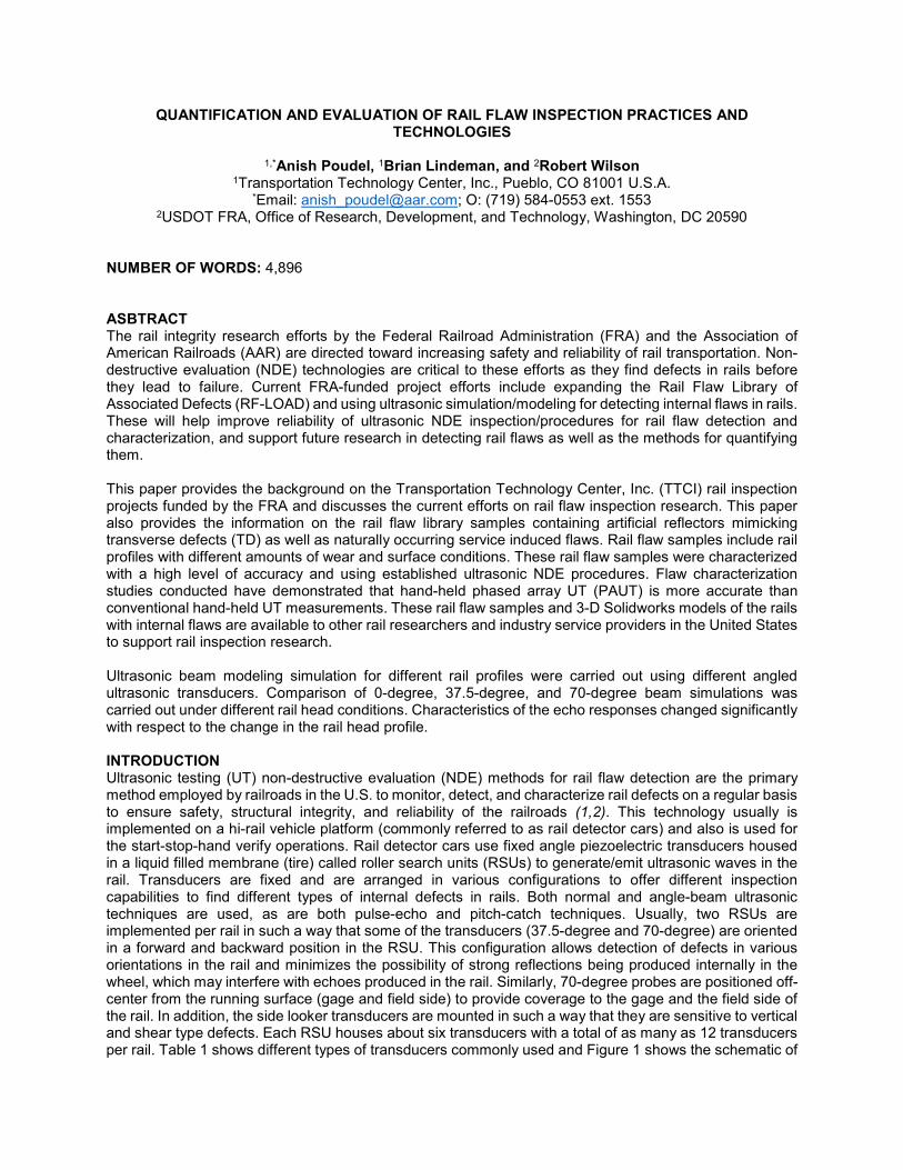
of the ultrasonic parameters considered to carry out this modeling and simulation work in CIVA UT. Some of the ultrasonic parameters used were provided by rail service providers while others were assumed (probe signal type, bandwidth, phase, and probe positioning) for this work. Hanning window function was applied and a typical 60 percent (-6dB) bandwidth was considered. Figure 6 shows the probe signal modeled for 3.5 MHz zero degree (0 degree) and 2.25 MHz 70 degree (70 degree) single-element flat-type rectangular immersion transducer. One thing that was noticeable prior to conducting ultrasonic simulation was the lower sampling rate (sampling frequency) for both probes. In order to reach an acceptable signal reconstruction, it is always recommended that the sample rate should be approximately 25 times its central frequency (f). The choice of low sampling frequency might lead to loss of signal information while a high sampling frequency increases storage and computation, hence identifying the appropriate sampling frequency is a critical factor for onset determination. Similarly, the number of points just needs to be large enough so that the signal at starting and ending times is close to zero. Fast automated ultrasonic inspections can be performed at 8-bit data sampling frequencies up to 500 MHz with data transfer rates of 20 Mbyte/sec or higher. These rates can be achieved with a dedicated PCI-ADC card installed in a standard PC.

Table 6. Ultrasonic and test parameters used for UT beam modeling and simulation.

UT Simulation Parameters Transducer Types 0° 37.5° 70° Center 70° Field 70° Gage CRYSTAL SHAPE

Dimension: Length/Width/Diameter [inch] 0.50/0.25 0.50/0.50 0.50/0.50 0.50/0.50 0.50/0.50

Wave Type: L-wave or S-wave L-wave S-wave S-wave S-wave S-wave

PROBE SIGNALS Center Frequency [MHz] 3.50 2.25 2.25 2.25 2.25

Bandwidth 60% @ -6 dB

60% @ -6 dB

60% @ -6 dB

60% @ -6 dB

60% @ -6 dB

Sampling Frequency [MHz] 25 25 25 25 25 Number of Points 256 256 256 256 256 PROBE POSITIONING

[with respect to the centerline of the rail head] location/ positioning Center Center Center Field Gage Offset from the centerline of the rail [inch] 0 0 0 0.63 0.63

Water Path distance [inch] 1 1 1 1 1 BEAM INFORMATION Incidence Angle (degrees) 0° 16.23° 25.56° 25.56° 25.56° Refracted Angle (degrees) 0° 37.5° 70° 70° 70°

(a) (b)

Figure 6. Modeled signal in CIVA UT. (a) 3.5 MHz 0-degree transducer; (b) and 2.25 MHz 70-degree transducer.

Similarly, the probe positioning inside the RSU (with fixed probe diameter and frequency) also plays an important role for optimal inspection. This determines the standoff (water path) distance from the probe to the rail. As a general rule of thumb, water path distance should be in excess of 25 percent the maximum beam path in the material for L-wave inspection and at least 50 percent of the beam path for S-wave inspection. However, for this work, the water path distance was set to 1 inch (25.4 mm) for all simulations. Beam Field Modeling Results Figure 7 shows the ray tracing and ultrasonic beam field computation results for individual transducers in the RSU. The first row in Figure 7 shows the ultrasonic beam ray path display for corresponding transducers in the rail. Similarly, the second row shows the computed 2D ultrasonic beam image field. It shows the maximum amplitude of the ultrasonic beam at any time in the computation zone (X-zone: lateral positioning of the transducer; Z-zone: depth). The amplitude of the ultrasonic beam at different depths in X-zone and Z-zone are shown in third and fourth rows, respectively.

(a) (b) (c)

Figure 7. RSU ultrasonic beam field computation (transmission) in 136RE rail. (a) 0-degree; (b) 37.5-degree and; (c) 70-degree ultrasonic transducers.

Examples, as shown in the third and fourth rows, depict the ultrasonic beam amplitude at 50-mm (2-inch) depth for the 0-degree transducer, at 100-mm (4-inch) depth for the 37.5-degree transducer, and at 25-mm (1-inch) depth for the 70-degree transducer. From these, it is evident that the intensity of the ultrasonic beam decreases with the depth. Therefore, optimal probe positioning and ultrasonic parameters are essential for the optimal inspection. Ray tracing and ultrasonic beam field computation results for individual transducers in the RSU shown in Figure 7 assume an ideal situation with un-worn/un-damaged railhead conditions. It is to be noted that with the increasing surface conditions and wear of the railhead, ultrasonic beam propagation in the rail can be severely affected.

Table 7. Ultrasonic beam transmission properties for 0° ultrasonic transducer.

Rail Sample

Beam deflection at interface (refraction)

Beam Spread Angle

Transducer Near Field [mm]

Focal Spot @ -6 dB

[mm x mm] Focal Spot Orientation

136 RE 0° 20.35° 41.46 37.6 x 12.5 90°

N 8.38° 20.59° 38.52 42.3 x 12.2 -1.9°

S 17.41° 20.41° 38.82 7.3 x 9.6 -11.3°

W 15.91° 21.45° 38.63 38.7 x 12.1 0.5°

(a) (b) (c) (d)

Figure 8. Ultrasonic beam field computation (transmission) of 0-degree ultrasonic transducer for different rail profiles. (a) 136 RE; (b) N-profile; (c) S-profile; (d) W-profile.

The next step was to understand the effect of varying rail profiles and surface conditions on the beam field responses for different transducers. Table 7 summarizes the refraction, beam spread angle, near field, and focal spot size and orientation of 0-degree ultrasonic beam transmission results for different rail profiles at -6dB. Figure 8 shows the ultrasonic beam field computation results for different rail profiles for 0-degree transducer. The 2-D image field shown in the first row is the maximum amplitude of the ultrasonic beam at any time in the computation zone (X-zone/Z-zone). Similarly, the maximum amplitude of the 0-degree

ultrasonic beam at 50 mm depth in X-zone and Z-zone for different rail profiles are also shown in second and third rows respectively in Figure 8. Table 8 summarizes the refraction, beam spread angle, near field, and focal spot size and orientation of 37.5-degree ultrasonic transducer for different rail profiles at -6dB. Ultrasonic beam field computation results of 37.5-degree transducer for different rail profiles are shown in Figure 9. It was observed that the ultrasonic beam amplitude decreased significantly when the impinging beam encounters the surface damaged rail profiles.

Table 8. Ultrasonic beam transmission properties for 37.5-degree transducer.

Rail Sample


Beam Spread Angle


Focal Spot @ -6 dB


136 RE 37.5° 18.08° 44.86 105 x 86 90°

N 37.9° 13.75° 51.97 86 x 70.5 90°

S 39.0° 20.99° 42.87 19.1 x 18.6 90°

W 38.7° 15.83° 47.15 46.2 x 39.6 90°

(a) (b) (c) (d)

Figure 9. Ultrasonic beam field computation (transmission) of 37.5-degree ultrasonic transducer

for different rail profiles. (a) 136 RE; (b) N-profile; (c) S-profile; (d) W-profile. Similarly, Table 9 summarizes the refraction, beam spread angle, near field, and focal spot size and orientation of 70-degree center ultrasonic transducer for different rail profiles at -6dB. Ultrasonic beam field computation results of 70-degree center transducer for different rail profiles are shown in Figure 10. As previously observed, the ultrasonic beam amplitude decreases in the surface damaged and worn rail profiles significantly.

Table 9. Ultrasonic beam transmission properties for 70-degree center ultrasonic transducer.

Rail Sample


Beam Spread Angle


Focal Spot @ -6 dB


136 RE 70° 19.93° 41.73 23.8 x 56 90°

N 70.47° 20.11° 41.5 20.2 x 47.1 90°

S 72.03° 19.95° 40.44 7.2 x 16.6 90°

W 71.69° 20.35° 41.19 12.4 x 30.5 90°

(a) (b) (c) (d)

Figure 10. Ultrasonic beam field computation (transmission) of 70-degree ultrasonic transducer for different rail profiles. (a) 136 RE; (b) N-profile; (c) S-profile; (d) W-profile.

Finally, Table 10 summarizes the refraction, beam spread angle, near field, and focal spot size and orientation of 70-degree gage side ultrasonic transducer for different rail profiles at -6dB. Ultrasonic beam field computation results of 70-degree gage transducer for different rail profiles are shown in Figure 11. As previously observed, the ultrasonic beam amplitude decreases in the surface damaged and worn rail profiles significantly. In case of the gage wear profile, the beam field cannot be computed as a result of ultrasonic attenuation and mode conversion.

Table 10. Ultrasonic beam transmission properties for 70-degree gage ultrasonic transducer.

Rail Sample


Beam Spread Angle


Focal Spot @ -6 dB


136 RE 71.41° 20.05° 45.26 90°

N 74.24° 20.2° 46.39 90°

S 77.07° 20.67° 47.67 90°

W N/A

(a) (b) (c) (d)

Figure 11. Ultrasonic beam field computation (transmission) of 70-degree Gage ultrasonic transducer for different rail profiles. (a) 136 RE; (b) N-profile; (c) S-profile; (d) W-profile.

CONCLUSIONS Master gage rail samples containing a variety of artificial reflectors mimicking TD type defects as well as naturally occurring rail flaw defects are being collected/developed at TTC. Rail flaw samples include varieties of rails (different sizes) with the normal head profiles (light headwear), surface damaged profiles, and curve worn (gage face wear) profiles obtained from HTL at FAST and from the revenue service. Precise characterization of the RF-LOAD samples was conducted using available physical and NDE measurement techniques. This allowed researchers to calculate wear (W1, W2, W3, gained and loss area) for each rail, align rails with the template profiles, and finally generate 2-D and 3-D Solidworks models of the rails. NDE analysis included hand-held conventional UT and PAUT characterization. From the UT characterizations, it was demonstrated that PAUT was more accurate than the conventional UT measurements for sizing reflectors (16-30 percent CSHA) located in the gage and field faces that were oriented 5 degrees and 10 degrees relative to the base. In some cases, it was extremely difficult to observe signals for reflectors in the gage and field faces using conventional UT for the curve worn rails. Zero-degree oriented FBHs (0.25 inch and 0.50 inch dia.) on the gage and field faces were almost impossible

to find using both PAUT/UT methods. However, the detectability increased when the FBHs were about 1-inch in diameter. Finally, the traditional approach of TD sizing using AREMA CSHA may not be valid for used or worn rails due to the head loss, which may cause under-estimating the size of the TD. Ultrasonic beam modeling for various ultrasonic transducers under different rail head profile conditions allowed characterization of the beam field of an ultrasonic transducer and visualization of the coverage of the beam field in the rail. It was determined that the ultrasonic beam amplitude decreased significantly in the surface damaged and worn rail profiles and was mainly attributed to the unwanted scattering and refraction of the ultrasonic wave. In the case of the gage wear profile, the beam field could not be computed as a result of severe ultrasonic attenuation and mode conversion. REFERENCES

1. Tuzik, B., 2019, “Faster, Smarter, Better Rail Flaw Testing,” Railway Track & Structures Magazine, pp. 12 -19.

2. Alahakoon, S., Sun, Y.Q., Spiryagin, M., and Cole, C., 2008, “Rail Flaw Detection Technologies for Safer, Reliable Transportation: A Review,” Journal of Dynamic Systems, Measurement, and Control, Vol. 140 (2): 020801-020801-17. doi: 10.1115/1.4037295.

3. Witte, M., Poudel, A., and Kalay, S., 2016, “Rail Flaw Characterization Using Phased Array Ultrasound,” Proc. of 25th ASNT Research Symposium, New Orleans, LA.

4. American Railway Engineering and Maintenance-of-Way Association (AREMA), 2014, Chapter 4 - Rail, Section 4.1, Field Rail Flaw Identification.

5. Mahaut, S., et al., 2010, “An overview of Ultrasonic beam propagation and flaw scattering models in the CIVA software,” AIP Conference Proceedings, vol. 1211, pp. 2133 -2140.

6. Lambert, J., et al., 2013, “A Fast Ultrasonic Simulation Tool based on Massively Parallel Implementations,” 40th Annual Review of Progress in Quantitative Nondestructive Evaluation, Baltimore, MD.

7. Deschamps, G. A., “Ray Techniques in Electromagnetics,” Proc. of IEEE, Vol. 60 (9), pp. 1022 - 1035, 1972.

8. Gengembre, N. and Lhémery, A., 2000, “Pencil Method in Elastodynamics: Application to Ultrasonic Field Computation,” Ultrasonics, Vol. 38 (1–8), pp. 495-499.

9. CIVA NDE User Manual, 2016. 10. Mahaut, S., et al., 2009, “Recent advances and current trends of ultrasonic modelling in CIVA,”

Insight, vol. 51(2). 11. Raillon, R. and Lecoeur-Taïbi, I., 2000, “Transient Elastodynamic Model for Beam Defect

Interaction: Application to Non-destructive Testing,” Ultrasonics, vol. 38(1- 8), pp. 527-530. 12. Dorval, V., et al., 2015, “Simulation of the UT Inspection of Planar Defects Using a Generic GTD-

Kirchhoff Approach,” Proc. of 41st Annual Review of Progress in QNDE, vol. 1650 (1), pp. 1750 – 1756.

Quantification & Evaluation of Rail Flaw Inspection

Practices and Technologies 1,*Anish Poudel, 1Brian Lindeman, and 2Robert Wilson

1Transportation Technology Center, Inc., Pueblo, CO 81001*Email: [email protected]; O: (719) 584-0553 ext. 1553

2USDOT FRA, Office of Research, Development, and Technology, Washington, DC 20590

mailto:[email protected]

TTCI Rail Flaw Detection ResearchUSDOT FRA

• Improving railroad safety through the reduction of rail failures and the associated risks of train derailments, while improving railroad economics by developing production or maintenance practices that increase rail service life.

AAR Strategic Research Initiatives• Improvement in reliability and safety of rail operations by

developing improved rail flaw detection methods as well as fostering the development of improved rail flaw detector systems.

Rail Flaws• Rail flaws develop from a number of causes. Mainly,

repeated cyclic loading can initiate defects at microscopic anomalies. Such defects will start and grow internally with accumulated

traffic (mileage and tonnage).

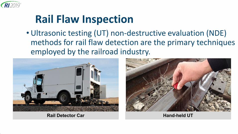
Rail Flaw Inspection• Ultrasonic testing (UT) non-destructive evaluation (NDE)

methods for rail flaw detection are the primary techniques employed by the railroad industry.

Rail Detector Car Hand-held UT

Rail Detector Cars • Rail detector cars use fixed angle piezoelectric transducers

housed in a liquid filled membrane (tire) called roller search units (RSUs) to generate/emit ultrasonic waves in the rail.

RSUs

Challenge• Inherent limitations of existing systems leave some

flaws being undetected (about 10 percent) during periodic inspections, which are only discovered after the rail breaks. • Misaligned RSU: Probes

and their inspection zone shift relative to rail

• Rail Wear: Angle shifted away from the target inspection zone

A True Collaborative Approach

Rail Flaw Library of Associated Defects (RF-LOAD)

Current Status• Artificial Reflectors: 54• Service Induced flaws

(TD/ DF/ VSH/BHC): 31• No Flaws: 30• Broken weld samples

(Web/Base Defects): 7Rail flaw samples are characterized with higher level of accuracy and standards.

Rail Flaw Library of Associated Defects (RF-LOAD)

Superimposed rail head profile showing different amounts of rail wear

RF-LOAD Flaw Sizing• Traditional approach of TD sizing using AREMA CSHA may not

be valid for severe worn rails due to the head loss, which may cause under-estimating the size of the TD.

𝑻𝑻𝑻𝑻 =𝝅𝝅 𝒍𝒍 𝒘𝒘𝟒𝟒 𝑨𝑨

× 𝟏𝟏𝟏𝟏𝟏𝟏𝟏

Measured Rail Head Area

[inch2]

AREMA Rail Head Area

[inch2]

Square End Mill Diameter

[inch]

Defect Orientation Relative to Base

[degrees]

TD Sizing - Measured CSHA

[%]

TD Sizing - AREMA CSHA

[%]Difference

4.19 4.82 1.25 5° 29.3% 25.5% 3.8%

4.14 4.82 1.25 10° 29.7% 25.5% 4.2%

Rail IDPhysical Measurements

W2

W3

W: Curve worn (gage face wear) TD located in Gage side

RF-LOAD UT Flaw Sizing

• PAUT sizing more accurate than the traditional hand-held UT for RF-LOAD samples.

Defect Orientation [degrees]

Actual TD Sizing

[%]

TD Location

Measured TD[%]

Measured TD[%]

5° 16.4% Center 17.5% 1% 2.8% 14%

10° 16.4% Center 19.0% 3% 4.0% 12%

5° 25.7% Gage 26.7% 1% 8.8% 17%

10° 27.6% Gage 27.0% 1% 8.2% 19%

5° 29.3% Gage 26.5% 3% 13.8% 16%

10° 29.7% Gage 30.5% 1% 13.0% 17%W2

Rail ID

Min

imal

He

ad

Wea

r

Surfa

ce

Dam

age

Gag

e Fa

ce

Wea

r W1

S1

S2

N2

N1

Physical Measurements PAUT Measurements%

Difference

Conventional UT Measurements%

Difference

Rail Flaw UT Modeling and Simulation• To better understand ultrasonic beam and probe

responses for commonly missed flaws (shape, size, orientations) in revenue service under different inspection scenarios.

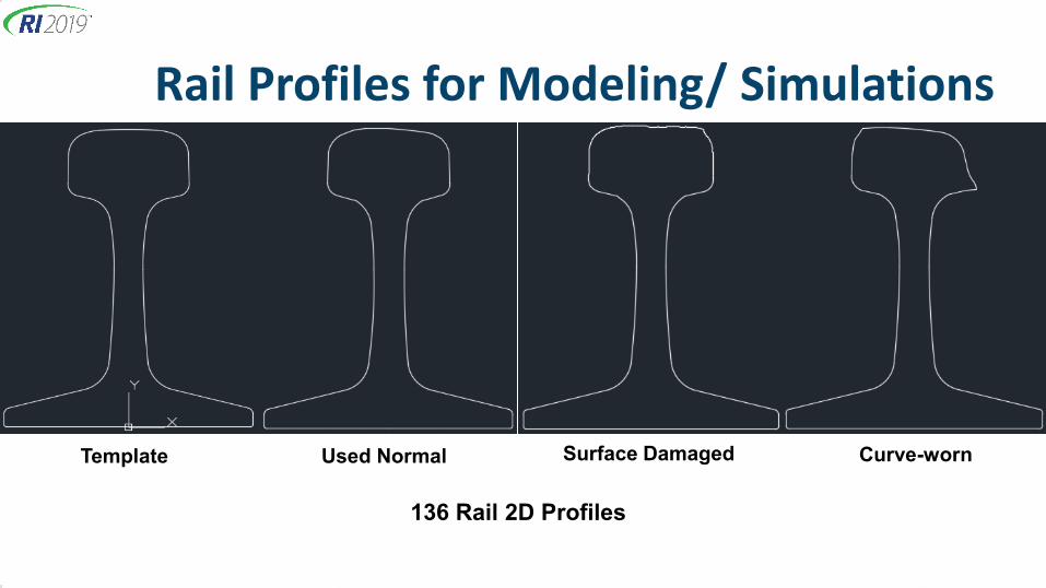
Rail Profiles for Modeling/ Simulations

Template Used Normal Surface Damaged Curve-worn

136 Rail 2D Profiles

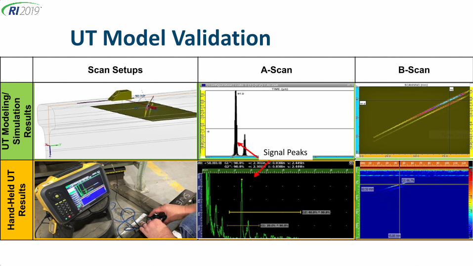
UT Model ValidationScan Setups A-Scan B-Scan

UT

Mod

elin

g/

Sim

ulat

ion

Res

ults

Han

d-H

eld

UT

Res

ults

Signal Peaks

UT Modeling and Simulation – 0°

Template Used Normal Surface Damaged Curve-worn

BeamRefraction

= 0°

BeamRefraction

= 8.38°

BeamRefraction

= 17.41°

BeamRefraction

= 15.91°

Rail profiles, surface damages (RCF), wear affects ultrasonic beam propagation

UT Modeling and Simulation - 37.5°

Template Used Normal Surface Damaged

Curve-worn

BeamRefraction

= 37.5°

BeamRefraction

= 37.9°

BeamRefraction

= 39.0°

BeamRefraction

= 38.7°


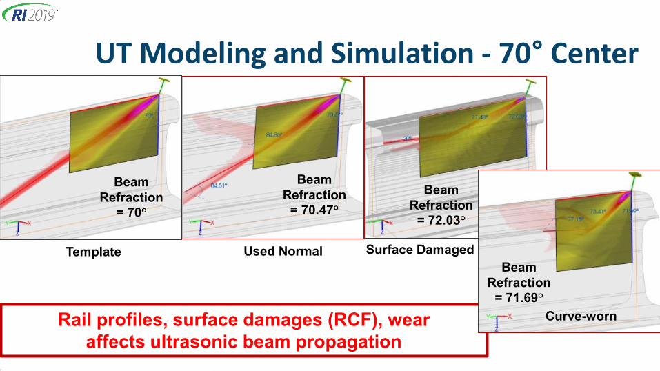
UT Modeling and Simulation - 70° Center


BeamRefraction

= 70°

BeamRefraction

= 70.47°Beam

Refraction= 72.03°


Curve-worn

BeamRefraction

= 71.69°

UT Modeling and Simulation - 70° Gage


BeamRefraction

= 71.41°

BeamRefraction

= 74.24°

BeamRefraction

= 77.07°


BeamRefraction

= N/ACurve-worn

Conclusions• Rail Flaw Library being developed at TTCI. PAUT was more accurate than the conventional UT measurements for flaw

sizing. Zero-degree oriented FBHs (0.25 inch and 0.50 inch dia.) on the gage and field

faces were almost impossible to find using both PAUT/UT methods. However, the detectability increased when the FBHs were about 1-inch in diameter. Traditional approach of TD sizing using AREMA CSHA may not be valid for used

or worn rails due to the head loss, which may cause under-estimating the size of the TD.

• Rail profiles, surface damages (RCF), wear affects ultrasonic beam propagation.

Thank you!

Documents

QUANTIFICATION AND EVALUATION OF RAIL FLAW …